Maps, Lies and Storytelling | P06 & P07| SQL & CartoCSS

Transcript

1. Maps, Lies & Storytelling Class 4
2. Welcome!
3. homework
4. Maps, Lies & Storytelling Section 6 - Learning SQL
5. SQL in CartoDB Can be viewed as the entry point for complex geospatial analysis, tool building, and data manipulation
6. Common SQL Statements SELECT UPDATE INSERT DELETE * there are lots of that we wont get into ** these can (and often are) mixed
7. Breaking down a SELECT statement
8. SELECT * FROM us_states The FROM statement tells us which table we are selecting data from
9. SELECT * FROM us_states The “*” here means, select ALL fields (or columns)
10. SELECT cartodb_id, name FROM us_states Here, I’ve opted to select only two columns specifically
11. SELECT cartodb_id, name FROM us_states The result of this query will have just the two columns I ask for, but for every row in my dataset cartodb_id name 1 new york 2 alabama etc
12. Here, I can limit it to just one column. SELECT cartodb_id FROM us_states cartodb_id 1 2 etc Notice that the result contains the column name
13. You can create an ‘alias’ for the result. Basically, change the name it uses for the result. SELECT cartodb_id AS my_id FROM us_states my_id 1 2 etc Notice that the results are the same, just a different name
14. You can modify values on the fly using SQL, for example, simple arithmetic. SELECT cartodb_id + 4 AS id FROM us_states id 5 6 etc The result isn’t stored anywhere permanently, it is derived on the fly
15. You can use a type of function, called an ‘Aggregate’ that measures across all rows at once. SELECT min(cartodb_id) AS id FROM us_states id 1 Now, only 1 row is returned
16. You can use a type of function, called an ‘Aggregate’ that measures across all rows at once. SELECT sum(cartodb_id) FROM us_states sum 1328 Now, only 1 row is returned
17. You can make up columns out of thin air. ! Notice that andrew is single quoted. That is the standard for strings SELECT cartodb_id, ‘andrew’ FROM us_states notice that ‘andrew’ remains constant for all rows cartodb_id unknown 1 andrew 2 andrew etc
18. Filtering using WHERE
19. Using WHERE statements will allow you to narrow in on exactly the rows you want SELECT cartodb_id FROM us_states WHERE cartodb_id = 1 cartodb_id 1 Here, only the single matching row is returned
20. Using WHERE statements work on all types of data SELECT name FROM us_states WHERE name = ‘New York’ name New York See!
21. When using string columns, they case sensitive SELECT name FROM us_states WHERE name = ‘new york’ name oh no! no results
22. Using WHERE statements will allow you to narrow in on exactly the rows you want SELECT cartodb_id FROM us_states WHERE cartodb_id > 24 cartodb_id 25 26 etc
23. You aren’t limited to using values as they exist, you can manipulate them on the fly SELECT cartodb_id FROM us_states WHERE cartodb_id*4=20 cartodb_id 5
24. With strings, you can do things like case insensitive partial matching. Here, ‘%’ is a wildcard, and ILIKE says use the wild card and ignore case SELECT name FROM us_states WHERE name ILIKE ‘new%’ name New Hampshire New Jersey etc Nice!
25. You can check if a value is in a set of options SELECT cartodb_id FROM us_states WHERE cartodb_id IN (1,4,99) name 1 4 Not 99 states
26. Always watch your quotes! ‘text’
27. Constrain results with ORDER BY & LIMIT
28. The LIMIT restricts the number or rows you ask for SELECT cartodb_id FROM us_states WHERE cartodb_id > 24 LIMIT 1 cartodb_id 25 see!
29. The LIMIT restricts the number or rows you ask for SELECT cartodb_id FROM us_states WHERE cartodb_id > 24 LIMIT 2 cartodb_id 25 26 see!
30. The ORDER BY allows you to change the order of rows in your result SELECT cartodb_id FROM us_states WHERE cartodb_id > 24 ORDER BY cartodb_id cartodb_id 25 26 etc The default is determined by the order on disk. no noticeable change here
31. ASC means, ascending. SELECT cartodb_id FROM us_states WHERE cartodb_id > 24 ORDER BY cartodb_id ASC cartodb_id 25 26 etc Here, ascending is the same as what we saw before
32. DESC means, descending SELECT cartodb_id FROM us_states WHERE cartodb_id > 24 ORDER BY cartodb_id DESC cartodb_id 52 51 etc See!
33. It works just as well on the alphabet SELECT name FROM us_states ORDER BY name DESC name Wyoming Wisconsin etc See!
34. USING GROUP BY
35. Let’s do something crazy here, substring() SELECT substring(name,1,3) FROM us_states substring Ala Ala Ari etc So we are asking for the first 3 characters of the state name
36. We can add a GROUP BY, which will join all rows with the same results SELECT substring(name,1,2) FROM us_states GROUP BY substring(name,1,2) substring Ala Ari Ark etc The second ‘Ala’ disappeared from our results
37. We can now use an aggregate that will work within each group result, not across the who table SELECT substring(name,1,2), count(*) FROM us_states GROUP BY substring(name,1,2) substring count Ala 2 Ari 1 Ark 1 etc Now we can see where that second ‘Ala’ went to!
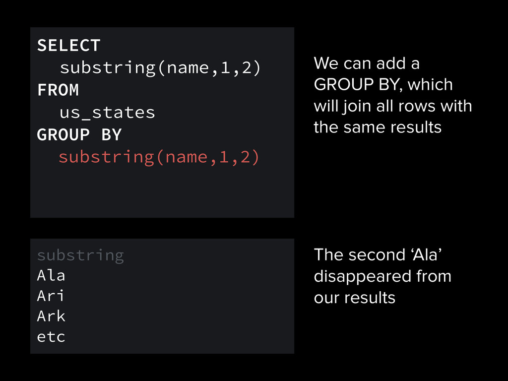
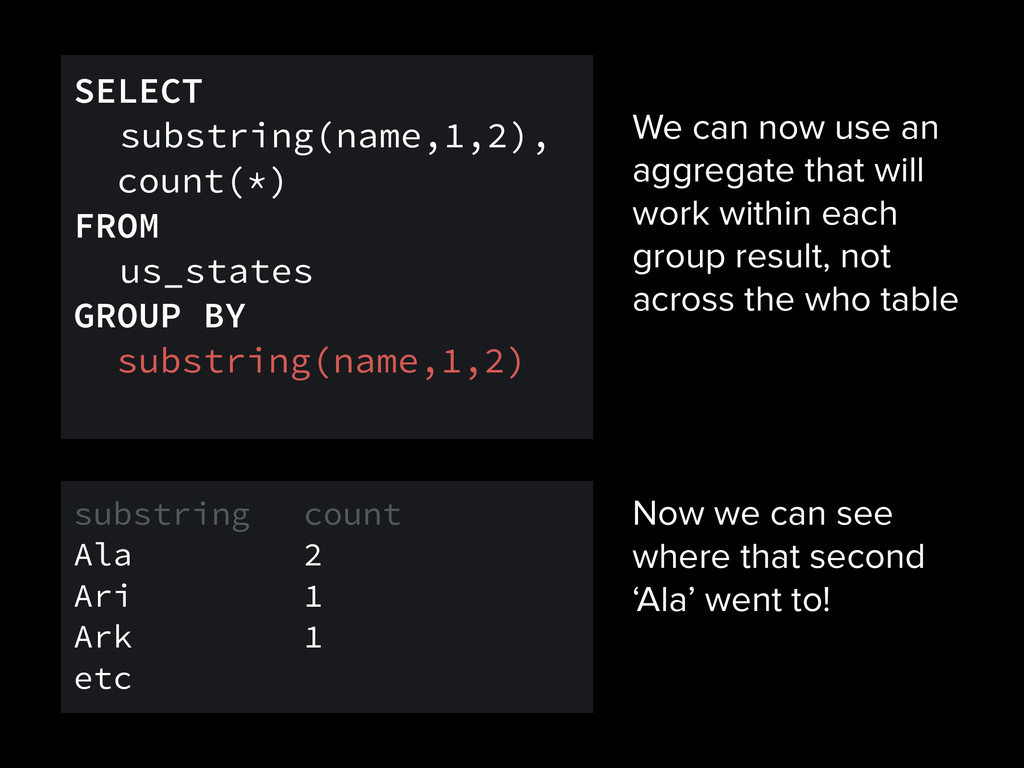
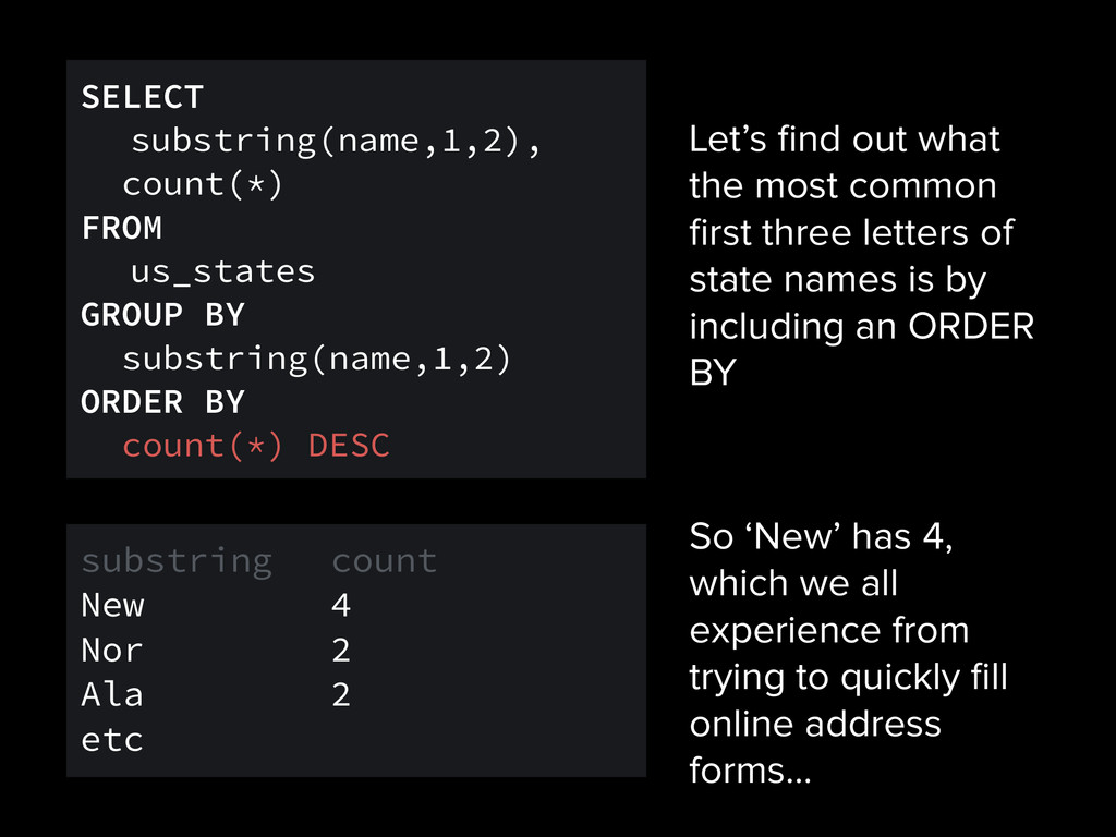
38. Let’s find out what the most common first three letters of state names is by including an ORDER BY SELECT substring(name,1,2), count(*) FROM us_states GROUP BY substring(name,1,2) ORDER BY count(*) DESC substring count New 4 Nor 2 Ala 2 etc So ‘New’ has 4, which we all experience from trying to quickly fill online address forms…
39. SQL Joins to query across tables
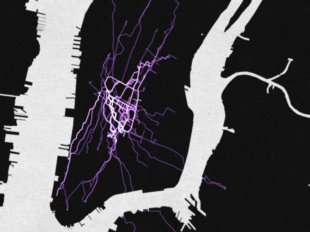
40. Someone else has done a really nice job of describing and illustrating this, so I’m going to shamelessly reuse
41. http://bit.ly/1vjVAUA
42. http://bit.ly/1vjVAUA
43. http://bit.ly/1vjVAUA
44. http://bit.ly/1vjVAUA
45. http://bit.ly/1vjVAUA
46. http://bit.ly/1vjVAUA
47. http://bit.ly/1vjVAUA
48. http://bit.ly/1vjVAUA
49. I also love nested queries
50. Here, I use a nested queries and compare against the results for a state name SELECT name, state FROM us_cities WHERE state IN (SELECT name FROM us_states WHERE name ILIKE ‘new y%’) name state New York New York Albany New York Buffalo New York etc
51. You can also nest right in the column results! SELECT name, (SELECT population FROM us_census WHERE name = u.name) pop FROM us_cities u ORDER BY pop DESC name pop California 38000000 Texas 26000000 New York 20000000 etc
52. The CTE or the “with” statement
53. You can use a WITH statement to treat a SQL result as a new table WITH fakestuff AS (SELECT name, state FROM us_cities WHERE name = ‘New York’) SELECT * FROM fakestuff name state New York New York Here, I create a magical new table- like object I call “fakestuff” When I select ‘*’ from the fakestuff table- ish thing, the result is only one row
54. I use them to help organize my thinking in SQL WITH fakestuff AS (SELECT ST_Centroid(the_geom) AS the_geom, name, pop FROM us_states) SELECT * FROM fakestuff WHERE pop > 5000000 name state New York New York
55. DELETES & UPDATES
56. UPDATES work with all the same properties of SELECT but with a few differences. UPDATE us_states SET name = ‘New Amsterdam’ WHERE name = ‘New York’ For example, you will only get a confirmation result, not actual rows. (typically)
57. Same goes for DELETE statements DELETE FROM us_states WHERE name = ‘New York’
59. An very basic introduction to spatial SQL
60. SELECT the_geom FROM us_states In CartoDB, your geometries are always standardized and stored in a column called the_geom the_geom MULTIPOLYGON… MULTIPOLYGON… etc
61. SELECT the_geom FROM us_states ORDER BY the_geom ASC You can manipulate, filter, order, measure and lots of other things to geometries the_geom MULTIPOLYGON… MULTIPOLYGON… etc
62. SELECT the_geom FROM us_states WHERE ST_Intersects(the_geom, my_geometry) CartoDB uses PostGIS to enable most geospatial functions. These are the functions that start with ‘ST_…’ the_geom MULTIPOLYGON…
63. SELECT the_geom FROM us_states WHERE ST_Intersects(the_geom, CDB_(42, -80)) We also have a couple of helper functions only in CartoDB, these start with CDB_. For example, CDB_LatLng(num, num) creates a geometry from two coordinates the_geom MULTIPOLYGON…
64. SELECT the_geom FROM us_states WHERE ST_Intersects(the_geom, CDB_(42, -80)) ST_Intersects returns TRUE if the two geometries intersect one another
65. SELECT the_geom FROM us_states WHERE ST_DWithin(the_geom, CDB_(42, -80), 1) ST_DWithin returns TRUE if the two geometries are within a minimum distance (supplied as the 3rd variable)
66. SELECT the_geom FROM us_states WHERE ST_DWithin(the_geom, CDB_(42, -80), 1) In CartoDB, we rely on projections. Using functions where we supply a unit measurement, that unit is always in the unit of the projection. Here, 1 degree lat/lng. Somewhat meaningless.
67. SELECT the_geom FROM us_states WHERE ST_DWithin(the_geom::geography, CDB_LatLng(42, -80)::geography, 10000) You can use a spherical globe and measure in meters by re-casting the geometries to geography types (on the fly)
68. SELECT the_geom FROM us_states ORDER BY the_geom <-> CDB_LatLng(44,-80) You can ORDER BY the distance to a specified geometry really nicely in CartoDB using <->
69. SELECT *, ST_Distance(the_geom, CDB_LatLng(42,-80)) AS d FROM us_states You can also use spatial measurements to derive a new or modified column result on the fly
70. SELECT *, ST_Distance(the_geom, CDB_LatLng(42,-80)) AS d FROM us_states ST_Distance will give me back the distance between two geometries. Here, the geometry in every row of my table would be measured from the point 42, -80
71. SELECT *, ST_Distance(the_geom::geography, CDB_LatLng(42,-80)::geography) AS d FROM us_states Remember, this returns a unit, so we might want to ensure we get meters
72. SELECT name, ST_MakeLine(the_geom, CDB_LatLng(42,-80)) AS the_geom FROM us_cities You can use ST_MakeLine to create lines between points on the fly. Here, I’ll turn every city point, into a line between that point and my point at 42, -80
73. UPDATE us_cities SET the_geom = ST_MakeLine(the_geom, CDB_LatLng(42,-80)) AS the_geom You can use all the stuff in UPDATES to store results as well. If I ran this, my cities would no longer be points, but would be lines! Careful, there is no UNDO!
74. SELECT name, ST_Centroid(the_geom) AS the_geom FROM us_states Likewise, we can turn polygons or lines into points. There are multiple ways to do this. ST_Centroid is one
75. SELECT name, ST_Envelope(the_geom) AS the_geom FROM us_cities GROUP BY state Or you could turn points into a polygon. ST_Envelope will create the minimum box around a group of points
76. the_geom versus the_geom_webmercator
77. the_geom the_geom_webmercator the_geom_webmercator When you create new data, it goes into, Behind the scenes, CartoDB also translates it to, When CartoDB draws a map, it comes from,
78. the_geom the_geom_webmercator Measure using Latitude, Longitude with,
79. the_geom the_geom_webmercator Select data to “Create new table” and include,
80. the_geom the_geom_webmercator Select or filter data you want on the map, include,
81. the_geom the_geom_webmercator CartoDB can’t render the map without
82. the_geom the_geom_webmercator Anytime you modify and store data on CartoDB will update so your maps are accurate,
83. the_geom the_geom_webmercator If you modify on the fly and want to map results, you need to create on the fly also!
84. SELECT cartodb_id, the_geom, the_geom_webmercator FROM us_states ORDER BY the_geom <-> CDB_LatLng(44,-80) You can do any filter you want, just make sure you include the_geom_webmercator in your column results to show it on the map
85. SELECT cartodb_id, ST_Buffer(the_geom, 1) FROM us_cities This wont display anything on your map, because it lacks the_geom_webmercator
86. SELECT cartodb_id, ST_Buffer(the_geom, 1), the_geom_webmercator FROM us_cities This would show the original points, but it would fail to include the transformed (buffered) point because the_geom hasn’t been altered on disk
87. SELECT cartodb_id, ST_Buffer(the_geom, 1) AS the_geom_webmercator FROM us_cities Just aliasing to the_geom_webmercator wont work, remember the_geom is a different projection than the_geom_webmercator
88. SELECT cartodb_id, ST_Transform(ST_Buffer(the_geom, 1), 3857) AS the_geom_webmercator FROM us_cities ST_Transform to the rescue!
89. SELECT cartodb_id, ST_Transform(ST_Buffer(the_geom, 1), 3857) AS the_geom_webmercator FROM us_cities ST_Transform turns projects any geometry from one projection to another. We want to go from WGS84 (the_geom) to Web Mercator (the_geom_webmercator)
90. SELECT cartodb_id, ST_Transform(ST_Buffer(the_geom, 1), 3857) AS the_geom_webmercator FROM us_cities In CartoDB, webmercator has an ID, or a SRID to be exact, that we can use to tell ST_Transform that we want webmercator from the_geom. The SRID is 3857 3857 = Web Mercator
91. SELECT cartodb_id, ST_Transform(ST_Buffer(the_geom, 1), 3857) AS the_geom_webmercator FROM us_cities Now our result will be on the map dynamically!
92. You can update the SQL of any layer in your visualizations with the setSQL function ! layer.setSQL(“SELECT * FROM us_states WHERE name = ‘New Hampshire’”); In CartoDB.js http://bit.ly/1t8vK1i
93. http://bit.ly/short-sql Don’t forget, more SQL examples
94. Let’s look at some of this live!
95. Maps, Lies & Storytelling Part 7 - More on CartoCSS
96. Once you’ve got the things you want to render, you will define a set of rules in CartoCSS to define how you render it
97. CartoCSS in CartoDB Can be viewed as the entry point for cartography and design
98. a few of the basics
99. #table{ polygon-fill: #FF6600; polygon-opacity: 0.7; line-color: #FFF; line-width: 1; line-opacity: 1; }
100. #table{ polygon-fill: red; polygon-opacity: 0.7; line-color: #FFF; line-width: 1; line-opacity: 1; }
101. #table{ polygon-fill: rgb(0,0,256); polygon-opacity: 0.7; line-color: #FFF; line-width: 1; line-opacity: 1; }
102. #table{ polygon-fill: #AEFF39; polygon-opacity: 0.2; line-color: #FFF; line-width: 1; line-opacity: 1; }
103. #table{ polygon-fill: #E94C6F; polygon-opacity: 0.9; line-color: #542733; line-width: 4; line-opacity: 1; }
104. #table{ marker-fill-opacity: 0.9; marker-line-color: #FFF; marker-line-width: 1.5; marker-line-opacity: 1; marker-placement: point; marker-type: ellipse; marker-width: 10; marker-fill: #FF6600; marker-allow-overlap: true; }
105. #table{ marker-fill-opacity: 0.9; marker-line-color: #FFF; marker-line-width: 1.5; marker-line-opacity: 1; marker-placement: point; marker-type: ellipse; marker-width: 22; marker-fill: #FF6600; marker-allow-overlap: true; }
106. #table{ marker-fill-opacity: 0.9; marker-line-color: yellow; marker-line-width: 3.5; marker-line-opacity: 1; marker-placement: point; marker-type: ellipse; marker-width: 22; marker-fill: #FF6600; marker-allow-overlap: true; }
107. lines use the same rules as the line borders of polygons
108. #table{ line-color: #FF6600; line-width: 2; line-opacity: 0.7; }
109. #table{ line-color: #FF6600; line-width: 15; line-opacity: 0.7; }
110. #table{ line-color: #FF6600; line-width: 15; line-opacity: 0.7; line-smooth: .5; }
111. #table{ line-color: #FF6600; line-width: 15; line-opacity: 0.7; line-smooth: 5.5; }
112. #table{ line-color: #FF6600; line-width: 15; line-opacity: 0.7; line-smooth: 5.5; line-dasharray: 5, 4; }
113. all of these are subject to composite operations. we’ll see in the hands on
114. Using rules
115. Any column in your table (or SQL result) can be used to define a rule
116. #table{ marker-fill-opacity: 0.9; marker-line-color: yellow; marker-line-width: 1.5; marker-line-opacity: 1; marker-width: 22; marker-fill: #FF6600; [atype = 'Specialized']{ marker-fill: white; } } ‘atype’ is a string column in my table
117. #table{ marker-fill-opacity: 0.9; marker-line-color: yellow; marker-line-width: 1.5; marker-line-opacity: 1; marker-width: 22; marker-fill: #FF6600; [atype = 'Specialized']{ marker-fill: white; } [atype = 'Institutional']{ marker-fill: green; } } ordered
118. #table{ marker-fill-opacity: 0.9; marker-line-color: blue; marker-line-width: 1.5; marker-line-opacity: 1; marker-width: 22; marker-fill: #FF6600; [atype = 'Institutional']{ marker-fill: green; [cartodb_id<12594]{ marker-line-color: red; } } } nested
119. #table{ marker-fill-opacity: 0.9; marker-line-color: blue; marker-line-width: 1.5; marker-line-opacity: 1; marker-width: 22; marker-fill: #FF6600; [is_valid = True]{ marker-fill: green; } } Boolean columns a slightly different in notation
120. Zoom as a parameter
121. #table{ marker-fill-opacity: 0.9; marker-line-color: blue; marker-line-width: 1.5; marker-line-opacity: 1; marker-width: 22; marker-fill: #FF6600; [zoom > 7]{ marker-line-width: 3; } } The zoom parameter
122. #table{ marker-fill-opacity: 0.9; marker-line-color: blue; marker-line-width: 1.5; marker-line-opacity: 1; marker-width: 22; marker-fill: #FF6600; [zoom > 7]{ marker-line-width: 3; [zoom > 8]{ marker-line-width: 6; } } } nested
123. A whole world of labels and text…
124. http://bit.ly/1rtx6pt
125. Client side CartoCSS | Torque
126. Client side CartoCSS | Torque
127. Map { -torque-frame-count:512; -torque-animation-duration:30; -torque-time- attribute:"cartodb_id"; -torque-aggregation- function:"count(cartodb_id)"; -torque-resolution:2; -torque-data- aggregation:linear; } The ‘Map’ object sets up the entire canvas and settings of your temporal visualization
128. Map { -torque-frame-count:512; -torque-animation-duration:30; -torque-time- attribute:"cartodb_id"; -torque-aggregation- function:"count(cartodb_id)"; -torque-resolution:2; -torque-data- aggregation:linear; } frame-count is how many temporal bins your data will be broken into. if you are visualizing 31 days, you wouldn’t need more than 31…
129. Map { -torque-frame-count:512; -torque-animation-duration:30; -torque-time- attribute:"cartodb_id"; -torque-aggregation- function:"count(cartodb_id)"; -torque-resolution:2; -torque-data- aggregation:linear; } duration is how long the animation will play for before looping back to the beginning
130. Map { -torque-frame-count:512; -torque-animation-duration:30; -torque-time- attribute:"cartodb_id"; -torque-aggregation- function:"count(cartodb_id)"; -torque-resolution:2; -torque-data- aggregation:linear; } time-attribute is the numerical or temporal column in your dataset that you want to order the animation by, beginning to end
131. Map { -torque-frame-count:512; -torque-animation-duration:30; -torque-time- attribute:"cartodb_id"; -torque-aggregation- function:"count(cartodb_id)"; -torque-resolution:2; -torque-data- aggregation:linear; } the aggregation- function is actually SQL! It is how you want data in the same spatial cell, in the same temporal bin, to be combined. here, you just get a raw value
132. Map { -torque-frame-count:512; -torque-animation-duration:30; -torque-time- attribute:"cartodb_id"; -torque-aggregation- function:"sum(population)"; -torque-resolution:2; -torque-data- aggregation:linear; } But here, you would get a totally different value. The result of this is an attribute called value that we can use to style with in our CartoCSS later
133. Map { -torque-frame-count:512; -torque-animation-duration:30; -torque-time- attribute:"cartodb_id"; -torque-aggregation- function:"count(cartodb_id)"; -torque-resolution:2; -torque-data- aggregation:linear; } resolution is the size of each pixel you will style
134. #table{ comp-op: lighter; marker-fill-opacity: 0.9; marker-line-color: #FFF; marker-line-width: 1.5; marker-line-opacity: 1; marker-type: ellipse; marker-width: 6; marker-fill: #FF9900; } Much of the CartoCSS for the rest looks the same as we saw before.
135. #table{ comp-op: lighter; marker-fill-opacity: 0.9; marker-line-color: #FFF; marker-line-width: 1.5; marker-line-opacity: 1; marker-type: ellipse; marker-width: 6; marker-fill: #FF9900; [value > 3]{ marker-fill-color: blue; } } We can use the value attribute from our aggregation function here to change styles though
136. #table[frame-offset=1] { marker-width:8; marker-fill-opacity:0.45; } We can also use frame-offsets ! frame-offsets allow you to draw the marker a second (or more times) after the frame it initially hits your maps.
137. You can update the CartoCSS of any layer in your visualizations with the setCartoCSS function (no line breaks) ! layer.setCartoCSS(“#tablename {marker- fill: red; }”); In CartoDB.js http://bit.ly/1vpF1pi
138. Maps, Lies & Storytelling Technology aside - Odyssey.js
139. hands on
140. Maps, Lies & Storytelling Guest speaker
141. Aurelia Moser Knight News Fellow Ushahidi / Internews http://aureliamoser.com/ Next week
142. Maps, Lies & Storytelling Discussion
143. Maps, Lies & Storytelling Assignments
144. Readings 5 Favorite Maps: Bill Rankin | http://bit.ly/1nrXEsV 15 Maps that explain ISIS | http://bit.ly/1pl02wx
145. I want you to show me the most far out way you can use CartoCSS and/or SQL to create a visualization. It can be a multistep process (UPDATEs, Table from Query), but be sure to document and share every step of your process. Assignment 1
146. Example 1
152. Example 2
154. Time to document your lie. Begin creating a comprehensive map and story of your lie. This should be a narrative story. During the narrative, you should highlight where your lie is exposed through maps. Assignment 2
155. Create a map to accompany a current news article or a current event. This should be an original map, not some improvement of a map included in the article Assignment 3
156. See you next week!