Deep Learning: An Introduction from the NLP Perspective by Kevin Duh

from http://cl.naist.jp/~kevinduh/notes/duh12deeplearn.pdf

Transcript

1. Deep Learning: An Introduction from the NLP Perspective Kevin Duh NAIST August 19, 2012
2. Introduction Neural Networks Deep Learning Approach 1 Deep Learning Approach 2 Disclaimer I am not (yet) an expert in Deep Learning. Let me know if these slides contain any mistakes. The focus here is Natural Language Processing (NLP); I’m glossing over much active work in Vision & Speech. Lots of good tutorial information online, some borrowed here: [Bengio, 2009] Excellent short book summarizing the area [Socher et al., 2012a] Tutorial with video Step-by-step code based on Theano python library: http://deeplearning.net/tutorial/ 2/43
3. Introduction Neural Networks Deep Learning Approach 1 Deep Learning Approach 2 Outline 1 Introduction 2 Neural Networks Preliminaries 1-Layer & 2-Layer Nets Neural Language Models 3 Deep Learning Approach 1: Deep Belief Nets Preliminaries Restricted Boltzman Machines Deep Belief Nets 4 Deep Learning Approach 2: Stacked Auto-Encoders Auto-Encoders Stacked Auto-Encoders Denoising Auto-Encoders and Variants 3/43
4. Introduction Neural Networks Deep Learning Approach 1 Deep Learning Approach 2 What is Deep Learning? A model (e.g. neural network) with many layers, trained in a layer-wise way 4/43
5. Introduction Neural Networks Deep Learning Approach 1 Deep Learning Approach 2 What is Deep Learning? A model (e.g. neural network) with many layers, trained in a layer-wise way An approach for unsupervised learning of feature representations, at successively higher levels 4/43
6. Introduction Neural Networks Deep Learning Approach 1 Deep Learning Approach 2 What is Deep Learning? A model (e.g. neural network) with many layers, trained in a layer-wise way An approach for unsupervised learning of feature representations, at successively higher levels These two definitions are very related, but correspond to different motivations. 4/43
7. Introduction Neural Networks Deep Learning Approach 1 Deep Learning Approach 2 Why explore Deep Learning? 1 It can model complex non-linear phenomenon 2 It learns a distributed feature representation 3 It learns a hierarchical feature representation 4 It can exploit unlabeled data 5/43
8. Introduction Neural Networks Deep Learning Approach 1 Deep Learning Approach 2 #1 Modeling complex non-linearities Given same number of units (with non-linear activation), a deeper architecture is more expressive than a shallow one [Bishop, 1995] 6/43
9. Introduction Neural Networks Deep Learning Approach 1 Deep Learning Approach 2 #2 Distributed Feature Representations One-hot representation is common in NLP: ”dog”=[1, 0, 0, . . . , 0], (vector dimension = vocabulary size) ”cat”=[0, 1, 0, . . . , 0] ”the”=[0, 0, 0, . . . , 1] ”dog” and ”cat” share zero similarity, just like ”dog” and ”the” 7/43
10. Introduction Neural Networks Deep Learning Approach 1 Deep Learning Approach 2 #2 Distributed Feature Representations One-hot representation is common in NLP: ”dog”=[1, 0, 0, . . . , 0], (vector dimension = vocabulary size) ”cat”=[0, 1, 0, . . . , 0] ”the”=[0, 0, 0, . . . , 1] ”dog” and ”cat” share zero similarity, just like ”dog” and ”the” Word clustering has proven effective in many tasks: ”dog”=[1, 0, 0, 0] (vector dim = number of clusters) ”cat”=[1, 0, 0, 0] (”dog” and ”cat” were clustered together) ”the”=[0, 1, 0, 0] dog,cat > dog,the = 0 7/43
11. Introduction Neural Networks Deep Learning Approach 1 Deep Learning Approach 2 #2 Distributed Feature Representations One-hot representation is common in NLP: ”dog”=[1, 0, 0, . . . , 0], (vector dimension = vocabulary size) ”cat”=[0, 1, 0, . . . , 0] ”the”=[0, 0, 0, . . . , 1] ”dog” and ”cat” share zero similarity, just like ”dog” and ”the” Word clustering has proven effective in many tasks: ”dog”=[1, 0, 0, 0] (vector dim = number of clusters) ”cat”=[1, 0, 0, 0] (”dog” and ”cat” were clustered together) ”the”=[0, 1, 0, 0] dog,cat > dog,the = 0 Distributed represented (= ”distributional representation”) is a multi-clustering, modeling factors like POS & semantics: ”dog”=[1, 0, 0.9, 0.0] ”cat”=[1, 0, 0.5, 0.2] ”the”=[0, 1, 0.0, 0.0] 7/43
12. Introduction Neural Networks Deep Learning Approach 1 Deep Learning Approach 2 #3 Hierarchical Feature Representations Hierarchical features effective captures part-and-whole relationships and naturally addresses multi-task problems [Lee et al., 2009] 8/43
13. Introduction Neural Networks Deep Learning Approach 1 Deep Learning Approach 2 #4 Exploiting Unlabeled Data Unsupervised & semi-supervised learning will be standard1: Engineering question: Unlabeled data is more abundant than labeled data. Scientific question: Children learn language (syntax, meaning, etc.) mostly from raw unlabeled data 1my prediction for 2020 9/43
14. Introduction Neural Networks Deep Learning Approach 1 Deep Learning Approach 2 #4 Exploiting Unlabeled Data Unsupervised & semi-supervised learning will be standard1: Engineering question: Unlabeled data is more abundant than labeled data. Scientific question: Children learn language (syntax, meaning, etc.) mostly from raw unlabeled data Layer-wise pre-training in Deep Learning: good model of input P(X) can help train P(Y |X) ”If you want to do computer vision, first learn computer graphics.” – Geoff Hinton 1my prediction for 2020 9/43
15. Introduction Neural Networks Deep Learning Approach 1 Deep Learning Approach 2 Some (personal) skepticism 10/43
16. Introduction Neural Networks Deep Learning Approach 1 Deep Learning Approach 2 Some (personal) skepticism 1 There are other ways to learn distributed representations, e.g. Topic model for documents Concatenating multiple word clustering solutions (has anyone tried this?) Dictionary learning and sparse reconstruction methods 10/43
17. Introduction Neural Networks Deep Learning Approach 1 Deep Learning Approach 2 Some (personal) skepticism 1 There are other ways to learn distributed representations, e.g. Topic model for documents Concatenating multiple word clustering solutions (has anyone tried this?) Dictionary learning and sparse reconstruction methods 2 Is multiple-level of representations really necessary in NLP? For Vision problems, there is clear analogy to the brain’s structure, but for language? Maybe: compositionally and recursion in natural language. 10/43
18. Introduction Neural Networks Deep Learning Approach 1 Deep Learning Approach 2 Some (personal) skepticism 1 There are other ways to learn distributed representations, e.g. Topic model for documents Concatenating multiple word clustering solutions (has anyone tried this?) Dictionary learning and sparse reconstruction methods 2 Is multiple-level of representations really necessary in NLP? For Vision problems, there is clear analogy to the brain’s structure, but for language? Maybe: compositionally and recursion in natural language. 3 Black magic required for effective training, e.g. hyper-parameter setting and large computer resources? 10/43
19. Introduction Neural Networks Deep Learning Approach 1 Deep Learning Approach 2 Research Opportunities in NLP 1 Improving on current state-of-the-art results on standard tasks 11/43
20. Introduction Neural Networks Deep Learning Approach 1 Deep Learning Approach 2 Research Opportunities in NLP 1 Improving on current state-of-the-art results on standard tasks 2 Encoding linguistic knowledge into the training process Current methods are relatively generic, incorporates little domain knowledge. 11/43
21. Introduction Neural Networks Deep Learning Approach 1 Deep Learning Approach 2 Research Opportunities in NLP 1 Improving on current state-of-the-art results on standard tasks 2 Encoding linguistic knowledge into the training process Current methods are relatively generic, incorporates little domain knowledge. 3 Integrating deep learning into current NLP pipelines In particular: how to handle structured prediction problems of sequences and trees 11/43
22. Introduction Neural Networks Deep Learning Approach 1 Deep Learning Approach 2 What we’ll cover here 1 Neural Language Models & Distributed Word Representations Not sure if they’re ”deep”, but they’re relevant to what we’re interested in Basic math here useful for later material 2 Restricted Boltzman Machines & Deep Belief Nets Deep Learning Approach #1: the original generative model 3 Autoencoders, Denoising Autoencoders, and Stacked Denoising Autoencoders Deep Learning Approach #2: competitive with #1 and perhaps easier to train 12/43
23. Introduction Neural Networks Deep Learning Approach 1 Deep Learning Approach 2 Aside: A Brief History Early days of AI. Invention of artificial neuron [McCulloch and Pitts, 1943] & perceptron [Rosenblatt, 1958] 13/43
24. Introduction Neural Networks Deep Learning Approach 1 Deep Learning Approach 2 Aside: A Brief History Early days of AI. Invention of artificial neuron [McCulloch and Pitts, 1943] & perceptron [Rosenblatt, 1958] AI Winter. [Minsky and Papert, 1969] showed perceptron only learns linearly separable concepts 13/43
25. Introduction Neural Networks Deep Learning Approach 1 Deep Learning Approach 2 Aside: A Brief History Early days of AI. Invention of artificial neuron [McCulloch and Pitts, 1943] & perceptron [Rosenblatt, 1958] AI Winter. [Minsky and Papert, 1969] showed perceptron only learns linearly separable concepts Revival in 1980s: Multi-layer Perceptrons (MLP) and Back-propagation [Rumelhart et al., 1986] 13/43
26. Introduction Neural Networks Deep Learning Approach 1 Deep Learning Approach 2 Aside: A Brief History Early days of AI. Invention of artificial neuron [McCulloch and Pitts, 1943] & perceptron [Rosenblatt, 1958] AI Winter. [Minsky and Papert, 1969] showed perceptron only learns linearly separable concepts Revival in 1980s: Multi-layer Perceptrons (MLP) and Back-propagation [Rumelhart et al., 1986] Other directions (1990s - present): SVMs, Bayesian Networks 13/43
27. Introduction Neural Networks Deep Learning Approach 1 Deep Learning Approach 2 Aside: A Brief History Early days of AI. Invention of artificial neuron [McCulloch and Pitts, 1943] & perceptron [Rosenblatt, 1958] AI Winter. [Minsky and Papert, 1969] showed perceptron only learns linearly separable concepts Revival in 1980s: Multi-layer Perceptrons (MLP) and Back-propagation [Rumelhart et al., 1986] Other directions (1990s - present): SVMs, Bayesian Networks Revival in 2006: Deep learning [Hinton et al., 2006] 13/43
28. Introduction Neural Networks Deep Learning Approach 1 Deep Learning Approach 2 Aside: A Brief History Early days of AI. Invention of artificial neuron [McCulloch and Pitts, 1943] & perceptron [Rosenblatt, 1958] AI Winter. [Minsky and Papert, 1969] showed perceptron only learns linearly separable concepts Revival in 1980s: Multi-layer Perceptrons (MLP) and Back-propagation [Rumelhart et al., 1986] Other directions (1990s - present): SVMs, Bayesian Networks Revival in 2006: Deep learning [Hinton et al., 2006] Recent successes in applications: Speech at IBM/Toronto [Sainath et al., 2011], Microsoft [Dahl et al., 2012]. Vision at Google/Stanford [Le et al., 2012] 13/43
29. Introduction Neural Networks Deep Learning Approach 1 Deep Learning Approach 2 Preliminaries 1-Layer & 2-Layer Nets Neural Language Models Outline 1 Introduction 2 Neural Networks Preliminaries 1-Layer & 2-Layer Nets Neural Language Models 3 Deep Learning Approach 1: Deep Belief Nets Preliminaries Restricted Boltzman Machines Deep Belief Nets 4 Deep Learning Approach 2: Stacked Auto-Encoders Auto-Encoders Stacked Auto-Encoders Denoising Auto-Encoders and Variants 14/43
30. Introduction Neural Networks Deep Learning Approach 1 Deep Learning Approach 2 Preliminaries 1-Layer & 2-Layer Nets Neural Language Models Basic Setup of Machine Learning Training Data: a set of (x(m), y(m))m={1,2,..M} pairs, where input x(m) ∈ Rd and output y(m) = {0, 1} e.g. x=document, y=spam or not Goal: Learn function f : x → y that predicts correctly on new inputs x. 15/43
31. Introduction Neural Networks Deep Learning Approach 1 Deep Learning Approach 2 Preliminaries 1-Layer & 2-Layer Nets Neural Language Models Basic Setup of Machine Learning Training Data: a set of (x(m), y(m))m={1,2,..M} pairs, where input x(m) ∈ Rd and output y(m) = {0, 1} e.g. x=document, y=spam or not Goal: Learn function f : x → y that predicts correctly on new inputs x. Step 1: Choose a function model family: e.g. f (x) = σ(wT · x). (logistic regression, aka. 1-layer net) e.g. f (x) =sign(wT · x). (perceptron) e.g. f (x) =sign m wT m · k(x, x(m)). (SVM) 15/43
32. Introduction Neural Networks Deep Learning Approach 1 Deep Learning Approach 2 Preliminaries 1-Layer & 2-Layer Nets Neural Language Models Basic Setup of Machine Learning Training Data: a set of (x(m), y(m))m={1,2,..M} pairs, where input x(m) ∈ Rd and output y(m) = {0, 1} e.g. x=document, y=spam or not Goal: Learn function f : x → y that predicts correctly on new inputs x. Step 1: Choose a function model family: e.g. f (x) = σ(wT · x). (logistic regression, aka. 1-layer net) e.g. f (x) =sign(wT · x). (perceptron) e.g. f (x) =sign m wT m · k(x, x(m)). (SVM) Step 2: Optimize parameters w on the Training Data e.g. minimize loss function minw M m=1 (fw (x(m)) − y(m))2 15/43
33. Introduction Neural Networks Deep Learning Approach 1 Deep Learning Approach 2 Preliminaries 1-Layer & 2-Layer Nets Neural Language Models 1-Layer Nets (logistic regression) Function model: f (x) = σ(wT · x + b) Parameters: vector w ∈ Rd , b is scalar bias term σ is a non-linearity: σ(z) = 1/(1 + exp(−z)) For simplicity, sometimes write f (x) = σ(wT x) where w = [w; b] and x = [x; 1] 16/43
34. Introduction Neural Networks Deep Learning Approach 1 Deep Learning Approach 2 Preliminaries 1-Layer & 2-Layer Nets Neural Language Models 1-Layer Nets (logistic regression) Function model: f (x) = σ(wT · x + b) Parameters: vector w ∈ Rd , b is scalar bias term σ is a non-linearity: σ(z) = 1/(1 + exp(−z)) For simplicity, sometimes write f (x) = σ(wT x) where w = [w; b] and x = [x; 1] Non-linearity will be important in expressiveness multi-layer nets. Other non-linearities are also used, e.g. tanh 16/43
35. Introduction Neural Networks Deep Learning Approach 1 Deep Learning Approach 2 Preliminaries 1-Layer & 2-Layer Nets Neural Language Models Training 1-Layer Nets Easiest method: gradient descent Let Loss(w) = m (σ(wT x(m)) − y(m))2 17/43
36. Introduction Neural Networks Deep Learning Approach 1 Deep Learning Approach 2 Preliminaries 1-Layer & 2-Layer Nets Neural Language Models Training 1-Layer Nets Easiest method: gradient descent Let Loss(w) = m (σ(wT x(m)) − y(m))2 Gradient ∇w Loss = m 2(σ(wT x(m)) − y(m))(σ(wT x(m))(1 − σ(wT x(m)))x(m) 17/43
37. Introduction Neural Networks Deep Learning Approach 1 Deep Learning Approach 2 Preliminaries 1-Layer & 2-Layer Nets Neural Language Models Training 1-Layer Nets Easiest method: gradient descent Let Loss(w) = m (σ(wT x(m)) − y(m))2 Gradient ∇w Loss = m 2(σ(wT x(m)) − y(m))(σ(wT x(m))(1 − σ(wT x(m)))x(m) General form of gradient: Error ∗ σ (in) ∗ x 17/43
38. Introduction Neural Networks Deep Learning Approach 1 Deep Learning Approach 2 Preliminaries 1-Layer & 2-Layer Nets Neural Language Models Training 1-Layer Nets Easiest method: gradient descent Let Loss(w) = m (σ(wT x(m)) − y(m))2 Gradient ∇w Loss = m 2(σ(wT x(m)) − y(m))(σ(wT x(m))(1 − σ(wT x(m)))x(m) General form of gradient: Error ∗ σ (in) ∗ x Stochastic gradient descent algorithm: 1 Initialize w 2 for each sample (x(m), y(m)) in training set 3 w ← w − γ(Error ∗ σ (in) ∗ x(m)) 4 Repeat steps 2-3 until some condition satisfied Some practical tricks for learning rate γ & stopping condition for quick training and good generalization 17/43
39. Introduction Neural Networks Deep Learning Approach 1 Deep Learning Approach 2 Preliminaries 1-Layer & 2-Layer Nets Neural Language Models 2-Layer Nets (MLP, Multi-layer Perceptron) x1 x2 x3 x4 h1 h2 h3 y xi wij hj wj w11 w12 w1 w2 w3 f (x) = σ( j wj · hj ) = σ( j wj · σ( i wij xi )) 18/43
40. Introduction Neural Networks Deep Learning Approach 1 Deep Learning Approach 2 Preliminaries 1-Layer & 2-Layer Nets Neural Language Models Training 2-Layer Nets: Backpropagation Recall the gradient for 1-Layer Nets consists of: ∂Loss/∂wj = Error ∗ σ (in) ∗ xj We just need to use Chain Rule to take derivatives over 2-layers 19/43
41. Introduction Neural Networks Deep Learning Approach 1 Deep Learning Approach 2 Preliminaries 1-Layer & 2-Layer Nets Neural Language Models Training 2-Layer Nets: Backpropagation Recall the gradient for 1-Layer Nets consists of: ∂Loss/∂wj = Error ∗ σ (in) ∗ xj We just need to use Chain Rule to take derivatives over 2-layers For the 2-Layer network (previous slide): ∂Loss/∂wj = [y − f (x)]f (x)hj ∂Loss/∂wij = [y − f (x)]f (x)wj σ ( i wi jxi )xi 19/43
42. Introduction Neural Networks Deep Learning Approach 1 Deep Learning Approach 2 Preliminaries 1-Layer & 2-Layer Nets Neural Language Models Training 2-Layer Nets: Backpropagation Recall the gradient for 1-Layer Nets consists of: ∂Loss/∂wj = Error ∗ σ (in) ∗ xj We just need to use Chain Rule to take derivatives over 2-layers For the 2-Layer network (previous slide): ∂Loss/∂wj = [y − f (x)]f (x)hj ∂Loss/∂wij = [y − f (x)]f (x)wj σ ( i wi jxi )xi Note: 1 First, run sample through network to get result f (x). 2 Then, ”errors” are propagated back and weights fixed according to their ”responsibility” 3 Problem is not convex (may have several local optima) 19/43
43. Introduction Neural Networks Deep Learning Approach 1 Deep Learning Approach 2 Preliminaries 1-Layer & 2-Layer Nets Neural Language Models Definition of ”Depth” Depends on elementary computational elements: weighted sum, product, single neuron, kernel, logic gate 1-Layer - linear classifier: Logistic Regression, Maximum Entropy Classifier Perceptron, Linear SVM 2-Layer - universal approximator: Most MLPs (except some convolutional neural nets) SVMs with kernels Gaussian processes Decision trees 3-Layer or more - compact universal approximator: Deep Learning Boosted decision trees, Random Forests 20/43
44. Introduction Neural Networks Deep Learning Approach 1 Deep Learning Approach 2 Preliminaries 1-Layer & 2-Layer Nets Neural Language Models Neural Language Models [Bengio et al., 2003] Motivation: Use Neural Nets to learn continuous distributed representations of words. Addresses curse of dimensionality arising from one-hot representation of discrete variables. Architecture (see pic on next slide): C() are the learned word representations of dimension m. The history context x = [C(wt−1 ) C(wt−2 ) C(wt−3 )] is compressed to a h node hidden layer via tanh(Hx) Final output mapping with softmax gives probabilities p(wt|x). 21/43
45. Introduction Neural Networks Deep Learning Approach 1 Deep Learning Approach 2 Preliminaries 1-Layer & 2-Layer Nets Neural Language Models Neural Language Models [Bengio et al., 2003] 22/43
46. Introduction Neural Networks Deep Learning Approach 1 Deep Learning Approach 2 Preliminaries 1-Layer & 2-Layer Nets Neural Language Models Distributed Representations: many possibilities 1 Neural Networks & Neural Language Model: Hidden layer serve as learned representation We can view this as analogous learning a kernel. 23/43
47. Introduction Neural Networks Deep Learning Approach 1 Deep Learning Approach 2 Preliminaries 1-Layer & 2-Layer Nets Neural Language Models Distributed Representations: many possibilities 1 Neural Networks & Neural Language Model: Hidden layer serve as learned representation We can view this as analogous learning a kernel. 2 Principle Component Analysis (PCA), Factor Analysis Linear transform to decorrelated features: h = W T x + b 3 Sparse coding h∗ = arg minh ||x − W · h||2 2 + λ||h||1 4 Also: manifold embeddings, ICA, and various unsupervised methods. 23/43
48. Introduction Neural Networks Deep Learning Approach 1 Deep Learning Approach 2 Preliminaries 1-Layer & 2-Layer Nets Neural Language Models Summary: things to remember about Neural Nets 1 Stacking layers of non-linearity (e.g. σ) is critical for expressive power of neural nets 2 Hidden layers of neural nets can serve as distributed representations 3 Backpropagation Training is just gradient descent, applied with Chain Rule. 4 Unfortunately, training beyond 2-layers is often difficult due to local optimum and vanishing gradients 24/43
49. Introduction Neural Networks Deep Learning Approach 1 Deep Learning Approach 2 Preliminaries 1-Layer & 2-Layer Nets Neural Language Models Minimal Reading List for Neural Language Models Original Neural LM paper: [Bengio et al., 2003] Alternate training criteria & architecture: [Collobert et al., 2011] Hierarchical distributed representations: [Mnih and Hinton, 2008] Handling large data (code available also): [Mikolov et al., 2011, Schwenk et al., 2012] Application in NLP: [Turian et al., 2010] 25/43
50. Introduction Neural Networks Deep Learning Approach 1 Deep Learning Approach 2 Preliminaries Restricted Boltzman Machines Deep Belief Nets Outline 1 Introduction 2 Neural Networks Preliminaries 1-Layer & 2-Layer Nets Neural Language Models 3 Deep Learning Approach 1: Deep Belief Nets Preliminaries Restricted Boltzman Machines Deep Belief Nets 4 Deep Learning Approach 2: Stacked Auto-Encoders Auto-Encoders Stacked Auto-Encoders Denoising Auto-Encoders and Variants 26/43
51. Introduction Neural Networks Deep Learning Approach 1 Deep Learning Approach 2 Preliminaries Restricted Boltzman Machines Deep Belief Nets Motivation Goal: Discover useful latent features h from data x 27/43
52. Introduction Neural Networks Deep Learning Approach 1 Deep Learning Approach 2 Preliminaries Restricted Boltzman Machines Deep Belief Nets Motivation Goal: Discover useful latent features h from data x One possibility: Directed Graphical Models: Model p(x, h) = p(x|h)p(h), where p(x|h) is likelihood, p(h) is prior Directed: we can think of h as a ”cause”. Given h = 1, what’s the probability of x? h x 27/43
53. Introduction Neural Networks Deep Learning Approach 1 Deep Learning Approach 2 Preliminaries Restricted Boltzman Machines Deep Belief Nets Explaining away effect of directed graphical models p(h1) and p(h2) are a priori independent, but dependent given x : p(h1, h2|x) = p(h1|x) · p(h2|x) Thus, posterior p(h|e), which is needed for features or deep learning, is not easy to compute Example: x = grass is wet; h1 = it rained last night; h2 = water sprinkler was on. x h1 h2 28/43
54. Introduction Neural Networks Deep Learning Approach 1 Deep Learning Approach 2 Preliminaries Restricted Boltzman Machines Deep Belief Nets Undirected Graphical Models (aka MRF, Markov Random Fields) MRF models p(x, h) = 1 Zθ i φi (x) j ηj (h) k νk(x, h) as product of un-normalized potentials θ are parameters, Zθ is (potentially expensive) normalization Clique potentials φi (x), ηj (h), νk (x, h) describe interactions between inputs, hiddens, and input-hidden variables 29/43
55. Introduction Neural Networks Deep Learning Approach 1 Deep Learning Approach 2 Preliminaries Restricted Boltzman Machines Deep Belief Nets Undirected Graphical Models (aka MRF, Markov Random Fields) MRF models p(x, h) = 1 Zθ i φi (x) j ηj (h) k νk(x, h) as product of un-normalized potentials θ are parameters, Zθ is (potentially expensive) normalization Clique potentials φi (x), ηj (h), νk (x, h) describe interactions between inputs, hiddens, and input-hidden variables Boltzman Machines define p(x, h) = 1 Zθ exp (−Eθ(x, h)) where x and h are binary variables, and Eθ (x, h) = −1 2 xT Ux − 1 2 hT Vh − xT Wh − bT x − dT h with θ = {U, V , W , b, d} as parameters 29/43
56. Introduction Neural Networks Deep Learning Approach 1 Deep Learning Approach 2 Preliminaries Restricted Boltzman Machines Deep Belief Nets Undirected Graphical Models (aka MRF, Markov Random Fields) MRF models p(x, h) = 1 Zθ i φi (x) j ηj (h) k νk(x, h) as product of un-normalized potentials θ are parameters, Zθ is (potentially expensive) normalization Clique potentials φi (x), ηj (h), νk (x, h) describe interactions between inputs, hiddens, and input-hidden variables Boltzman Machines define p(x, h) = 1 Zθ exp (−Eθ(x, h)) where x and h are binary variables, and Eθ (x, h) = −1 2 xT Ux − 1 2 hT Vh − xT Wh − bT x − dT h with θ = {U, V , W , b, d} as parameters Posterior p(h|x) of Boltzman Machines also intractable, e.g. p(hj |x) = h1 .. hj−1 hj+1 ..p(h|x). 29/43
57. Introduction Neural Networks Deep Learning Approach 1 Deep Learning Approach 2 Preliminaries Restricted Boltzman Machines Deep Belief Nets Restricted Boltzman Machine (RBM) RBM: p(x, h) = 1 Zθ exp (−Eθ(x, h)) with only h-x interactions: Eθ (x, h) = −xT Wh − bT x − dT h x1 x2 x3 h1 h2 h3 30/43
58. Introduction Neural Networks Deep Learning Approach 1 Deep Learning Approach 2 Preliminaries Restricted Boltzman Machines Deep Belief Nets Restricted Boltzman Machine (RBM) RBM: p(x, h) = 1 Zθ exp (−Eθ(x, h)) with only h-x interactions: Eθ (x, h) = −xT Wh − bT x − dT h x1 x2 x3 h1 h2 h3 Conditional distribution over hidden units factorizes: p(h|x) = i p(hi |x) p(hj = 1|x) = σ( i wij xi + dj ) Similarly: p(x|h) = i p(xi |h);p(xi = 1|h) = σ( j wij hj + bi ) Computing posteriors p(h|x) or features (E[p(h|x)) is easy. 30/43
59. Introduction Neural Networks Deep Learning Approach 1 Deep Learning Approach 2 Preliminaries Restricted Boltzman Machines Deep Belief Nets Restricted Boltzman Machine (RBM) RBM: p(x, h) = 1 Zθ exp (−Eθ(x, h)) with only h-x interactions: Eθ (x, h) = −xT Wh − bT x − dT h x1 x2 x3 h1 h2 h3 Conditional distribution over hidden units factorizes: p(h|x) = i p(hi |x) p(hj = 1|x) = σ( i wij xi + dj ) Similarly: p(x|h) = i p(xi |h);p(xi = 1|h) = σ( j wij hj + bi ) Computing posteriors p(h|x) or features (E[p(h|x)) is easy. Note partition function Zθ is still expensive, so approximation required during parameter learning 30/43
60. Introduction Neural Networks Deep Learning Approach 1 Deep Learning Approach 2 Preliminaries Restricted Boltzman Machines Deep Belief Nets Training RBMs Gradient of the Log-Likelihood: ∇w log Pw (x = x(m)) = ∇wij log h Pw (x = x(m), h) (1) = ∇wij log h 1 Zw exp (− Ew (x(m), h)) (2) = − ∇wij log Zw + ∇wij log h exp (− Ew (x(m), h)) (3) = 1 Zw h,x e(− Ew(x,h)) ∇wij Ew (x, h) − 1 h e(− Ew(x(m),h)) h e(− Ew(x(m),h)) ∇wij Ew (x(m), h) = h,x Pw (x, h)[∇wij Ew (x, h)] − h Pw (x(m), h)[∇wij Ew (x(m), h)] (4) = −Ep(x,h) [xi · hj ] + Ep(h|x=x(m)) [x(m) i · hj ] (5) 31/43
61. Introduction Neural Networks Deep Learning Approach 1 Deep Learning Approach 2 Preliminaries Restricted Boltzman Machines Deep Belief Nets Training RBMs with Contrastive Divergence In the previous equation, first term is expensive (Ep(x,h) [xi · hj ]) Gibbs Sampling (sample x then h iteratively) works but re-running for each gradient step is slow. Contrastive Divergence is a faster but biased method that initializes with training data: 1 ˆ h ∼ P(h|x(m)) 2 ˜ x ∼ P(x|ˆ h); ˜ h ∼ P(h|˜ x) 3 wij ← wij + γ batch (x(m) i · ˆ hj − ˜ xi · ˜ hj ) 32/43
62. Introduction Neural Networks Deep Learning Approach 1 Deep Learning Approach 2 Preliminaries Restricted Boltzman Machines Deep Belief Nets Deep Belief Nets (DBN) DBN stacks RBMs layer-by-layer to get deep architecture. Layer-wise pre-training is critical: First, train RBM to learn 1st layer of features h from input x. Then, treat h as input and learn a 2nd layer of features. Each added layer improves the variational lower bound on the log probability of training data. 33/43
63. Introduction Neural Networks Deep Learning Approach 1 Deep Learning Approach 2 Preliminaries Restricted Boltzman Machines Deep Belief Nets Deep Belief Nets (DBN) DBN stacks RBMs layer-by-layer to get deep architecture. Layer-wise pre-training is critical: First, train RBM to learn 1st layer of features h from input x. Then, treat h as input and learn a 2nd layer of features. Each added layer improves the variational lower bound on the log probability of training data. Further fine-tuning can be obtained with the Wake-Sleep Algorithm Do stochastic bottom-up pass (adjust weights to reconstruct layer below) Do a few iterations of Gibbs sampling at top-level RBM Do stochastic top-down pass (adjust weights to reconstruct layer above) note: not to be confused with Dynamic Bayesian Nets or Deep Boltzman Machines 33/43
64. Introduction Neural Networks Deep Learning Approach 1 Deep Learning Approach 2 Preliminaries Restricted Boltzman Machines Deep Belief Nets Summary: things to remember about DBNs 1 Layer-wise pre-training is the innovation that enabled training deep architectures. 2 Pre-training focuses on optimizing likelihood on the data, not the target label. The philosophy is to first model p(x) in order to do better p(y|x). 3 Why use an undirected graphical model like RBM? It’s because p(h|x) is computationally tractable (no ”explaining away effect”), so that stacking them into DBNs is feasible. 4 Learning RBM still require approximates inference (e.g. contrastive divergence) since partition function is expensive. 34/43
65. Introduction Neural Networks Deep Learning Approach 1 Deep Learning Approach 2 Preliminaries Restricted Boltzman Machines Deep Belief Nets Minimal Reading List for RBM/DBN Original DBN paper [Hinton et al., 2006] Why does unsupervised pre-training help deep learning? [Erhan et al., 2010] Successful application in Collaborative Filtering [Salakhutdinov et al., 2007] 35/43
66. Introduction Neural Networks Deep Learning Approach 1 Deep Learning Approach 2 Auto-Encoders Stacked Auto-Encoders Denoising Auto-Encoders and Variants Outline 1 Introduction 2 Neural Networks Preliminaries 1-Layer & 2-Layer Nets Neural Language Models 3 Deep Learning Approach 1: Deep Belief Nets Preliminaries Restricted Boltzman Machines Deep Belief Nets 4 Deep Learning Approach 2: Stacked Auto-Encoders Auto-Encoders Stacked Auto-Encoders Denoising Auto-Encoders and Variants 36/43
67. Introduction Neural Networks Deep Learning Approach 1 Deep Learning Approach 2 Auto-Encoders Stacked Auto-Encoders Denoising Auto-Encoders and Variants Auto-Encoders Auto-Encoders are a simpler non-probabilistic alternative to RBMs. Define encoder and decoder and pass the data through it: Encoder h = fθ (x), e.g. h = σ(Wx + b) Decoder x = gθ (h), e.g. x = σ(W h + d) W and W need not be tied, but often are in practice. 37/43
68. Introduction Neural Networks Deep Learning Approach 1 Deep Learning Approach 2 Auto-Encoders Stacked Auto-Encoders Denoising Auto-Encoders and Variants Auto-Encoders Auto-Encoders are a simpler non-probabilistic alternative to RBMs. Define encoder and decoder and pass the data through it: Encoder h = fθ (x), e.g. h = σ(Wx + b) Decoder x = gθ (h), e.g. x = σ(W h + d) W and W need not be tied, but often are in practice. Encourage θ to give small reconstruction errorl: e.g. Loss = m ||x(m) − gθ (fθ (x(m)))||2 37/43
69. Introduction Neural Networks Deep Learning Approach 1 Deep Learning Approach 2 Auto-Encoders Stacked Auto-Encoders Denoising Auto-Encoders and Variants Auto-Encoders Auto-Encoders are a simpler non-probabilistic alternative to RBMs. Define encoder and decoder and pass the data through it: Encoder h = fθ (x), e.g. h = σ(Wx + b) Decoder x = gθ (h), e.g. x = σ(W h + d) W and W need not be tied, but often are in practice. Encourage θ to give small reconstruction errorl: e.g. Loss = m ||x(m) − gθ (fθ (x(m)))||2 Linear encoder/decoder with squared reconstruction error learns same subspace of PCA. Sigmoid encoder/decoder gives same form p(h|x), p(x|h) as RBMs. 37/43
70. Introduction Neural Networks Deep Learning Approach 1 Deep Learning Approach 2 Auto-Encoders Stacked Auto-Encoders Denoising Auto-Encoders and Variants Architecture: Stacked Auto-Encoders Auto-encoders can be stacked in the same way RBMs are stacked to give Deep Architectures Hidden unit size: Hidden layer should be lower dimensional or else Auto-encoder may just learn the identity mapping Alternatively, allow more hidden units but enforce sparsity. 38/43
71. Introduction Neural Networks Deep Learning Approach 1 Deep Learning Approach 2 Auto-Encoders Stacked Auto-Encoders Denoising Auto-Encoders and Variants Denoising Auto-Encoders First, perturb the input data x to ˜ x using invariance from domain knowledge. Reconstruct the original data e.g. Loss = m ||x(m) − gθ (fθ (˜ x(m)))||2 [Vincent et al., 2010] explored Gaussian noise and salt-and-pepper noise for Vision data. [Glorot et al., 2011] explored masking noise (random set to 0) for Text data. 39/43
72. Introduction Neural Networks Deep Learning Approach 1 Deep Learning Approach 2 Auto-Encoders Stacked Auto-Encoders Denoising Auto-Encoders and Variants Predictive Sparse Decomposition [Kavukcuoglu et al., 2008] Objective (minimize with respect to h, W , θ): m λ||h(m)||1 + ||x(m) − Wh(m)||2 2 + ||h(m) − fθ(x(m))||2 2 First two terms similar to sparse coding. Third term learns a fast encoder that approximates the sparse coder. 40/43
73. Introduction Neural Networks Deep Learning Approach 1 Deep Learning Approach 2 Auto-Encoders Stacked Auto-Encoders Denoising Auto-Encoders and Variants Summary: things to remember about Stacked Autoencoders 1 Auto-encoders are computationally cheaper alternatives to RBMs. We stack them into deep architectures in the same way we stack RBMs into DBNs. 2 Auto-encoders learn to ”compress” and ”re-construct” input data. Low reconstruction error corresponds to an encoding that captures the main variations in data. Again, the focus is on modeling p(x) first. 3 Many variants of encoders are out there, and some provide effective ways to incorporate expertise domain knowledge. 41/43
74. Introduction Neural Networks Deep Learning Approach 1 Deep Learning Approach 2 Auto-Encoders Stacked Auto-Encoders Denoising Auto-Encoders and Variants Minimal Reading List for Stacked Auto-Encoders Original Stacked Auto-encoder paper [Bengio et al., 2006] Comparison of optimization methods [Le et al., 2011] Speeding up the reconstruction error computation for large word vectors [Dauphin et al., 2011] De-noising Auto-encoders [Vincent et al., 2010] 42/43
75. Introduction Neural Networks Deep Learning Approach 1 Deep Learning Approach 2 Auto-Encoders Stacked Auto-Encoders Denoising Auto-Encoders and Variants Selected Readings for NLPers Deep Learning Applications in NLP: Sentiment Analysis [Glorot et al., 2011] Parsing [Socher et al., 2011b, Collobert et al., 2011, Collobert, 2011] Paraphrase Detection [Socher et al., 2011a] Learning lexical semantics: [Huang et al., 2012, Socher et al., 2012b] Applications in other fields, but worth reading: Good reference that defines many terms popular in Deep Learning Vision papers [Jarrett et al., 2009] Deep learning of cats: entirely unsupervised learning high-level features on massive datasets [Le et al., 2012] 43/43
76. Introduction Neural Networks Deep Learning Approach 1 Deep Learning Approach 2 Auto-Encoders Stacked Auto-Encoders Denoising Auto-Encoders and Variants Bengio, Y. (2009). Learning Deep Architectures for AI, volume Foundations and Trends in Machine Learning. NOW Publishers. Bengio, Y., Ducharme, R., Vincent, P., and Jauvin, C. (2003). A neural probabilistic language models. JMLR. Bengio, Y., Lamblin, P., Popovici, D., and Larochelle, H. (2006). Greedy layer-wise training of deep networks. In NIPS’06, pages 153–160. Bishop, C. (1995). Neural Networks for Pattern Recognition. Oxford University Press. Collobert, R. (2011). 43/43
77. Introduction Neural Networks Deep Learning Approach 1 Deep Learning Approach 2 Auto-Encoders Stacked Auto-Encoders Denoising Auto-Encoders and Variants Deep learning for efficient discriminative parsing. In AISTATS. Collobert, R., Weston, J., Bottou, L., Karlen, M., Kavukcuoglu, K., and Kuksa, P. (2011). Natural language processing (almost) from scratch. Journal of Machine Learning Research, 12:2493–2537. Dahl, G., Yu, D., Deng, L., and Acero, A. (2012). Context-dependent pre-trained deep neural networks for large vocabulary speech recognition. IEEE Transactions on Audio, Speech, and Language Processing, Special Issue on Deep Learning for Speech and Langauge Processing. Dauphin, Y., Glorot, X., and Bengio, Y. (2011). Large-scale learning of embeddings with reconstruction sampling. In ICML’11, pages 945–952. 43/43
78. Introduction Neural Networks Deep Learning Approach 1 Deep Learning Approach 2 Auto-Encoders Stacked Auto-Encoders Denoising Auto-Encoders and Variants Erhan, D., Bengio, Y., Courville, A., Manzagol, P., Vincent, P., and Bengio, S. (2010). Why does unsupervised pre-training help deep learning? Journal of M, 11:625–660. Glorot, X., Bordes, A., and Bengio, Y. (2011). Domain adaptation for large-scale sentiment classication: A deep learning approach. In ICML. Hinton, G., Osindero, S., and Teh, Y.-W. (2006). A fast learning algorithm for deep belief nets. Neural Computation, 18:1527–1554. Huang, E., Socher, R., Manning, C., and Ng, A. (2012). Improving word representations via global context and multiple word prototypes. 43/43
79. Introduction Neural Networks Deep Learning Approach 1 Deep Learning Approach 2 Auto-Encoders Stacked Auto-Encoders Denoising Auto-Encoders and Variants In Proceedings of the 50th Annual Meeting of the Association for Computational Linguistics (Volume 1: Long Papers), pages 873–882, Jeju Island, Korea. Association for Computational Linguistics. Jarrett, K., Kavukcuoglu, K., Ranzato, M., and LeCun, Y. (2009). What is the best multi-stage architecture for object recognition? In Computer Vision, 2009 IEEE 12th International Conference on. Kavukcuoglu, K., Ranzato, M., and LeCun, Y. (2008). Fast inference in sparse coding algorithms with applications to object recognition. Technical Report CBLL-TR-2008-12-01, Computational and Biological Learning Lab, Courant Institute, NYU. 43/43
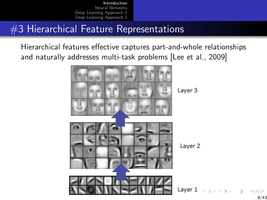
80. Introduction Neural Networks Deep Learning Approach 1 Deep Learning Approach 2 Auto-Encoders Stacked Auto-Encoders Denoising Auto-Encoders and Variants Le, Q., Ngiam, J., Coates, A., Lahiri, A., Prochnow, B., and Ng, A. (2011). On optimization methods for deep learning. In Getoor, L. and Scheffer, T., editors, Proceedings of the 28th International Conference on Machine Learning (ICML-11), ICML ’11, pages 265–272, New York, NY, USA. ACM. Le, Q. V., Ranzato, M., Monga, R., Devin, M., Chen, K., Corrado, G. S., Dean, J., and Ng, A. Y. (2012). Building high-level features using large scale unsupervised learning. In ICML. Lee, H., Grosse, R., Ranganath, R., and Ng, A. (2009). Convolutional deep belief networks for scalable unsupervised learning of hierarchical representations. In ICML. 43/43
81. Introduction Neural Networks Deep Learning Approach 1 Deep Learning Approach 2 Auto-Encoders Stacked Auto-Encoders Denoising Auto-Encoders and Variants McCulloch, W. S. and Pitts, W. H. (1943). A logical calculus of the ideas immanent in nervous activity. In Bulletin of Mathematical Biophysics, volume 5, pages 115–137. Mikolov, T., Deoras, A., Povey, D., Burget, L., and ˘ Cernock´ y, J. (2011). Strategies for training large scale neural network language model. In ASRU. Minsky, M. and Papert, S. (1969). Perceptrons: an introduction to computational geometry. MIT Press. Mnih, A. and Hinton, G. (2008). A scalable hierarchical distributed language models. In Advances in Neural Information Processing Systems 21 (NIPS 2008). 43/43
82. Introduction Neural Networks Deep Learning Approach 1 Deep Learning Approach 2 Auto-Encoders Stacked Auto-Encoders Denoising Auto-Encoders and Variants Rosenblatt, F. (1958). The perceptron: A probabilistic model for information storage and organization in the brain. Psychological Review, 65:386–408. Rumelhart, D. E., Hinton, G. E., and Williams, R. J. (1986). Learning representations by back-propagating errors. Nature, 323:533–536. Sainath, T. N., Kingsbury, B., Ramabhadran, B., Fousek, P., Novak, P., and Mohamed, A. (2011). Making deep belief networks effective for large vocabulary continuous speech recognition. In ASRU. Salakhutdinov, R., Mnih, A., and Hinton, G. (2007). Restricted boltzmann machines for collaborative filtering. 43/43
83. Introduction Neural Networks Deep Learning Approach 1 Deep Learning Approach 2 Auto-Encoders Stacked Auto-Encoders Denoising Auto-Encoders and Variants In Proceedings of the 24th international conference on Machine learning, ICML ’07, pages 791–798. Schwenk, H., Rousseau, A., and Attik, M. (2012). Large, pruned or continuous space language models on a gpu for statistical machine translation. In Proceedings of the NAACL-HLT 2012 Workshop: Will We Ever Really Replace the N-gram Model? On the Future of Language Modeling for HLT, pages 11–19, Montr´ eal, Canada. Association for Computational Linguistics. Socher, R., Bengio, Y., and Manning, C. (2012a). Deep learning for NLP (without the magic). ACL Tutorials http://www.socher.org/index.php/ DeepLearningTutorial/DeepLearningTutorial. Socher, R., Huang, E. H., Pennin, J., Ng, A. Y., and Manning, C. D. (2011a). 43/43
84. Introduction Neural Networks Deep Learning Approach 1 Deep Learning Approach 2 Auto-Encoders Stacked Auto-Encoders Denoising Auto-Encoders and Variants Dynamic pooling and unfolding recursive autoencoders for paraphrase detection. In NIPS. Socher, R., Huval, B., Manning, C. D., and Ng, A. Y. (2012b). Semantic compositionality through recursive matrix-vector spaces. In Proceedings of the 2012 Joint Conference on Empirical Methods in Natural Language Processing and Computational Natural Language Learning, pages 1201–1211, Jeju Island, Korea. Association for Computational Linguistics. Socher, R., Lin, C., Ng, A. Y., and Manning, C. D. (2011b). Parsing natural scenes and natural language with recursive neural networks. In ICML. Turian, J., Ratinov, L.-A., and Bengio, Y. (2010). 43/43
85. Introduction Neural Networks Deep Learning Approach 1 Deep Learning Approach 2 Auto-Encoders Stacked Auto-Encoders Denoising Auto-Encoders and Variants Word representations: A simple and general method for semi-supervised learning. In Proceedings of the 48th Annual Meeting of the Association for Computational Linguistics, pages 384–394, Uppsala, Sweden. Association for Computational Linguistics. Vincent, P., Larochelle, H., Lajoie, I., Bengio, Y., and Manzagol, P.-A. (2010). Stacked denoising autoencoders: Learning useful representations in a deep network with a local denoising criterion. Journal of Machine Learning Research, 11:3371–3408. 43/43