Markovian sequential decision-making in non-stationary environments: application to argumentation problems

markovian sequential decision-making in non-stationary environments application to argumentative debates
Emmanuel Hadoux director: Nicolas Maudet supervisors: Aurélie Beynier and Paul Weng November, 26th 2015 LIP6 / UPMC - ED 130

sequential decision-making problem? Example • What do I want to
eat? • Which color should I wear? • Which way to go to work? 2

sequential decision-making problem? Example • What do I want to
eat? (one shot) • Which color should I wear? (one shot) • Which way to go to work? (sequential) 2

sequential decision-making problem under uncertainty? A more precise deﬁnition An
agent (real or virtual) makes decisions in an environment. 3

agent (real or virtual) makes decisions in an environment. The state evolves with the actions performed by the agent. 3

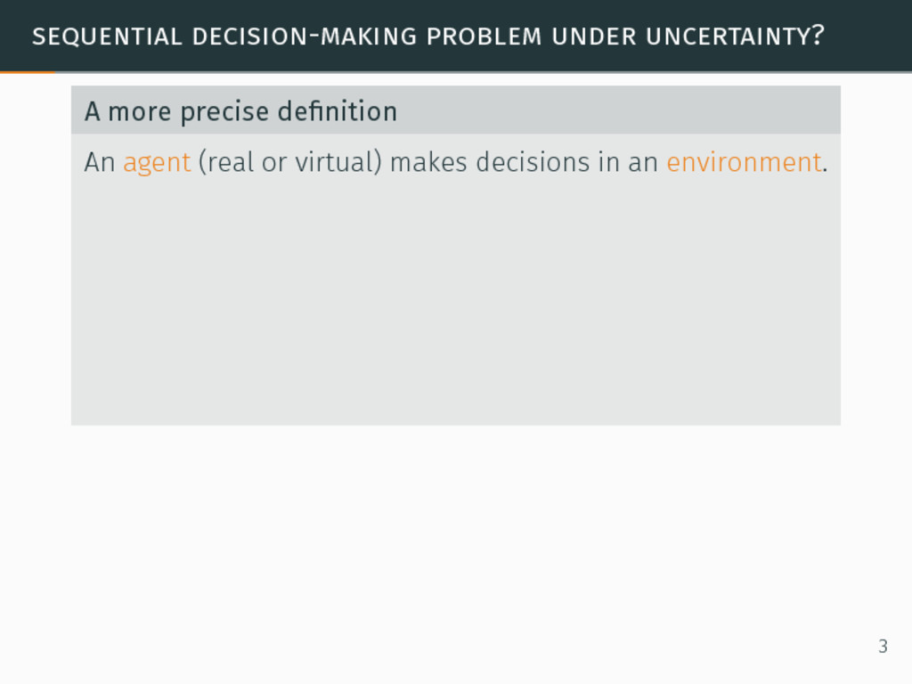
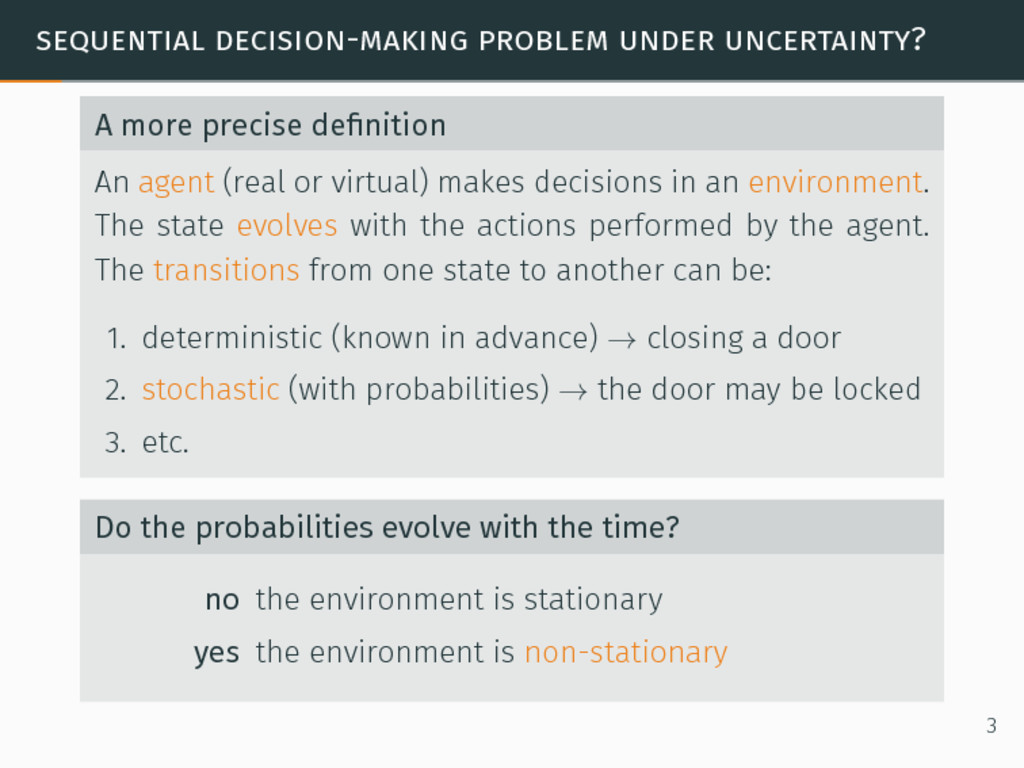
agent (real or virtual) makes decisions in an environment. The state evolves with the actions performed by the agent. The transitions from one state to another can be: 3

agent (real or virtual) makes decisions in an environment. The state evolves with the actions performed by the agent. The transitions from one state to another can be: 1. deterministic (known in advance) → closing a door 3

agent (real or virtual) makes decisions in an environment. The state evolves with the actions performed by the agent. The transitions from one state to another can be: 1. deterministic (known in advance) → closing a door 2. stochastic (with probabilities) → the door may be locked 3

agent (real or virtual) makes decisions in an environment. The state evolves with the actions performed by the agent. The transitions from one state to another can be: 1. deterministic (known in advance) → closing a door 2. stochastic (with probabilities) → the door may be locked 3. etc. 3

agent (real or virtual) makes decisions in an environment. The state evolves with the actions performed by the agent. The transitions from one state to another can be: 1. deterministic (known in advance) → closing a door 2. stochastic (with probabilities) → the door may be locked 3. etc. Do the probabilities evolve with the time? no the environment is stationary yes the environment is non-stationary 3

the whole context We are interested in: 1. Solving sequential
decision-making problem 4

decision-making problem 2. under uncertainty (with stochastic dynamics) 4

decision-making problem 2. under uncertainty (with stochastic dynamics) 3. in non-stationary environments 4

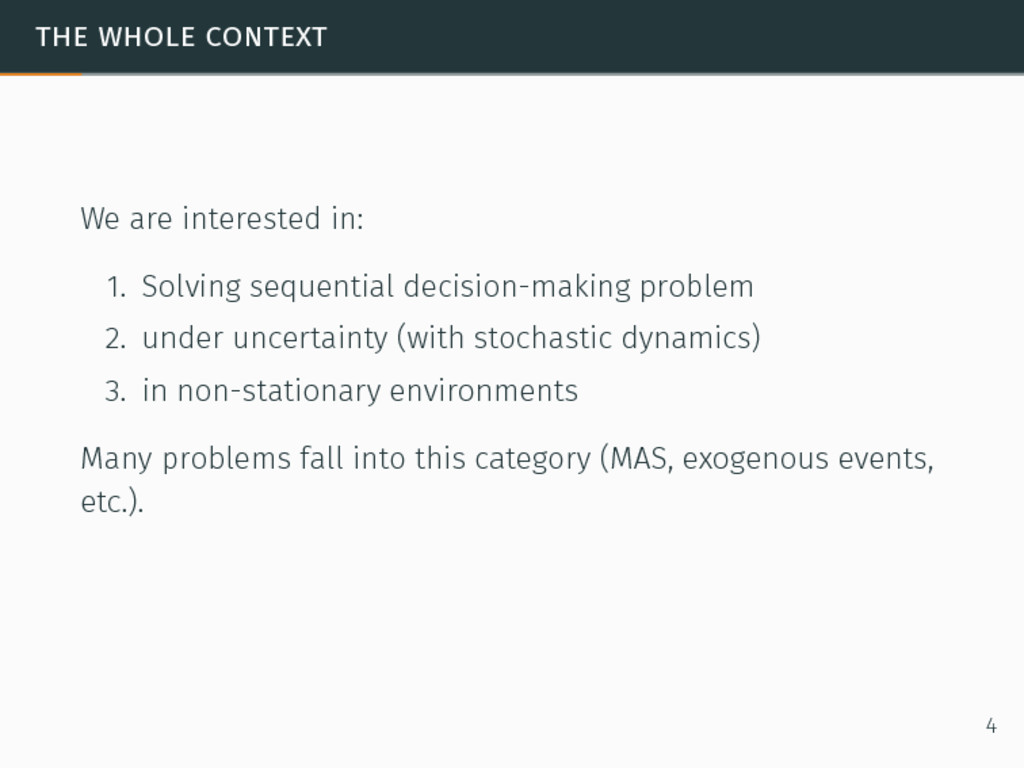
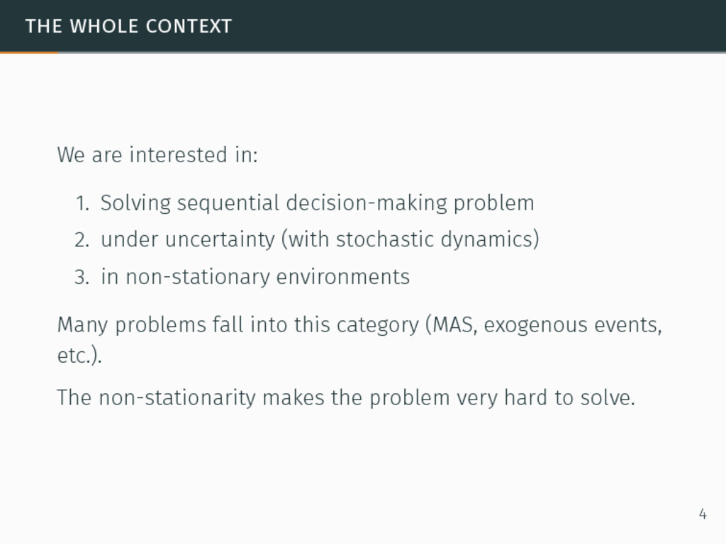
decision-making problem 2. under uncertainty (with stochastic dynamics) 3. in non-stationary environments Many problems fall into this category (MAS, exogenous events, etc.). 4

decision-making problem 2. under uncertainty (with stochastic dynamics) 3. in non-stationary environments Many problems fall into this category (MAS, exogenous events, etc.). The non-stationarity makes the problem very hard to solve. 4

table of contents Decision-making in non-stationary environments 1. Markov Decision
Models 2. Non-stationary environments Application to argumentation problems 1. Strategic debate 2. Mediation problems 5

markov decision models

markov decision process Markov Decision Process (MDP)1 ⟨S, A, T,
R⟩ such that: 1Martin L. Puterman. Markov Decision Processes: Discrete dynamic stochastic programming. John Wiley Chichester, 1994. 7

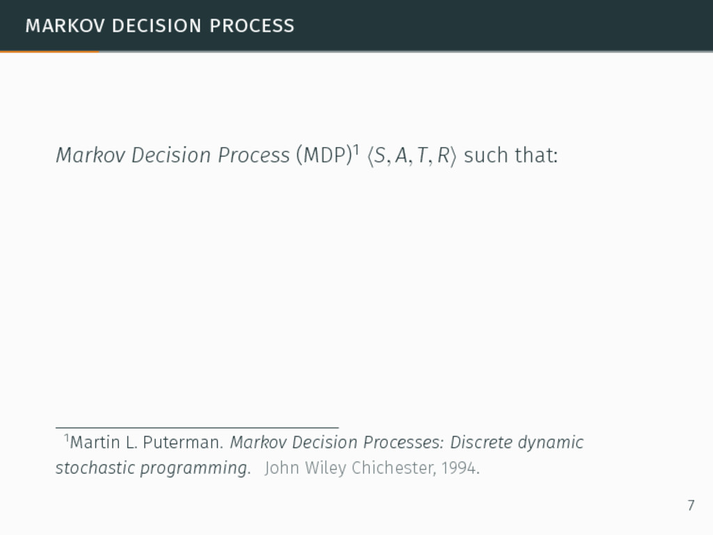
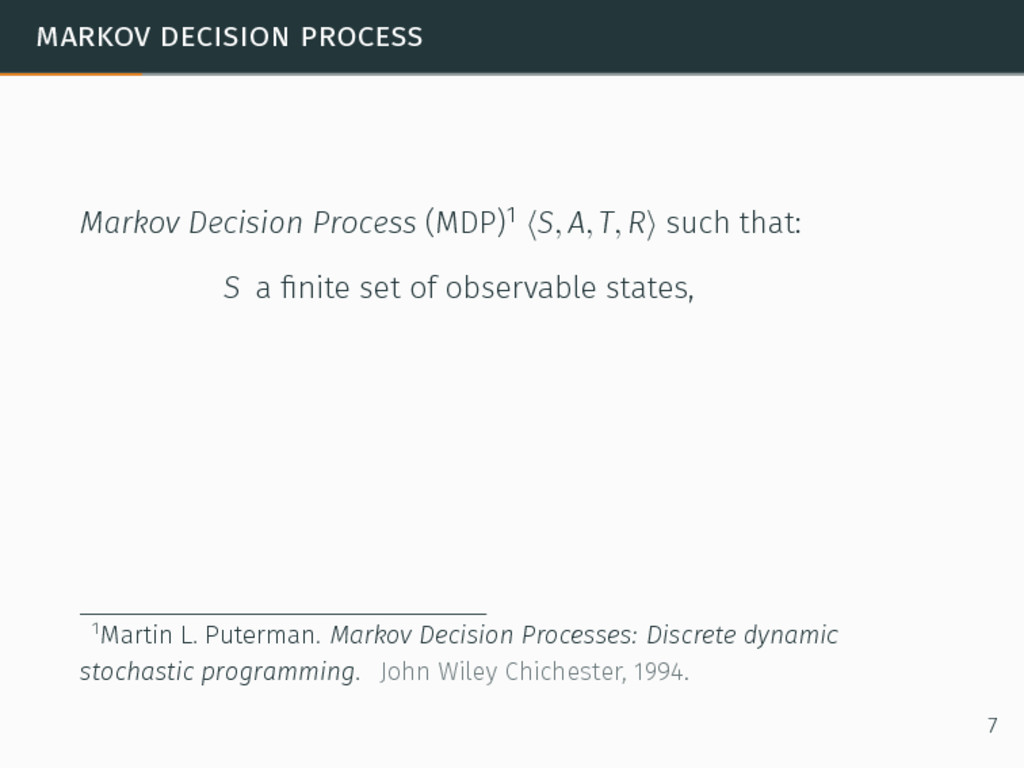
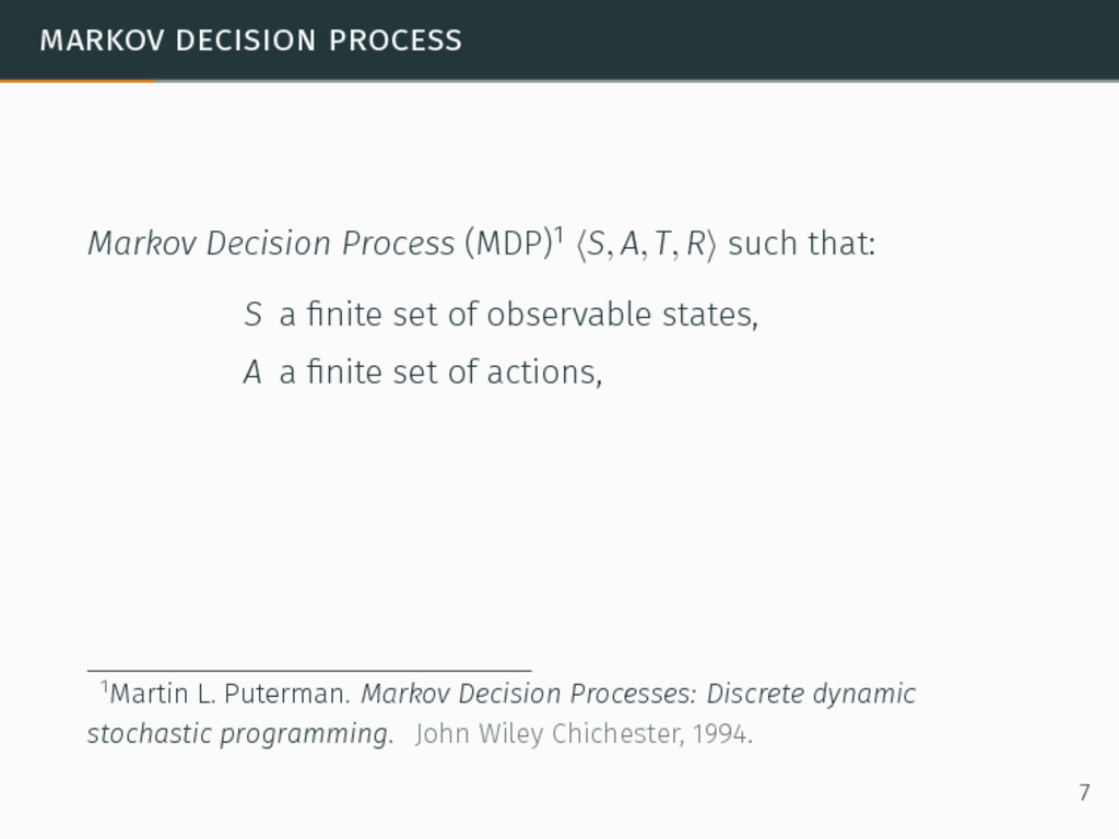
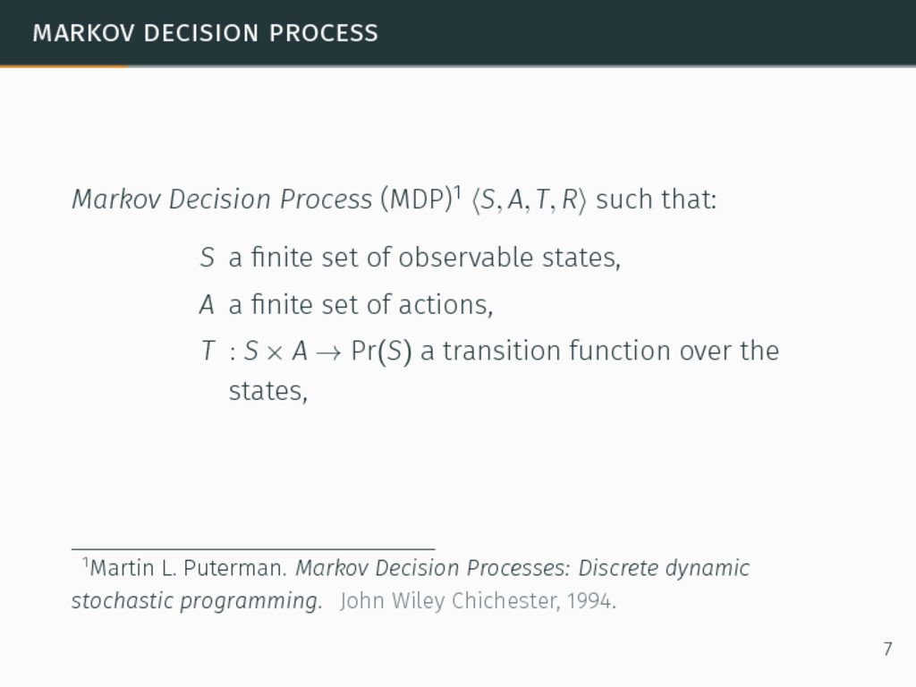
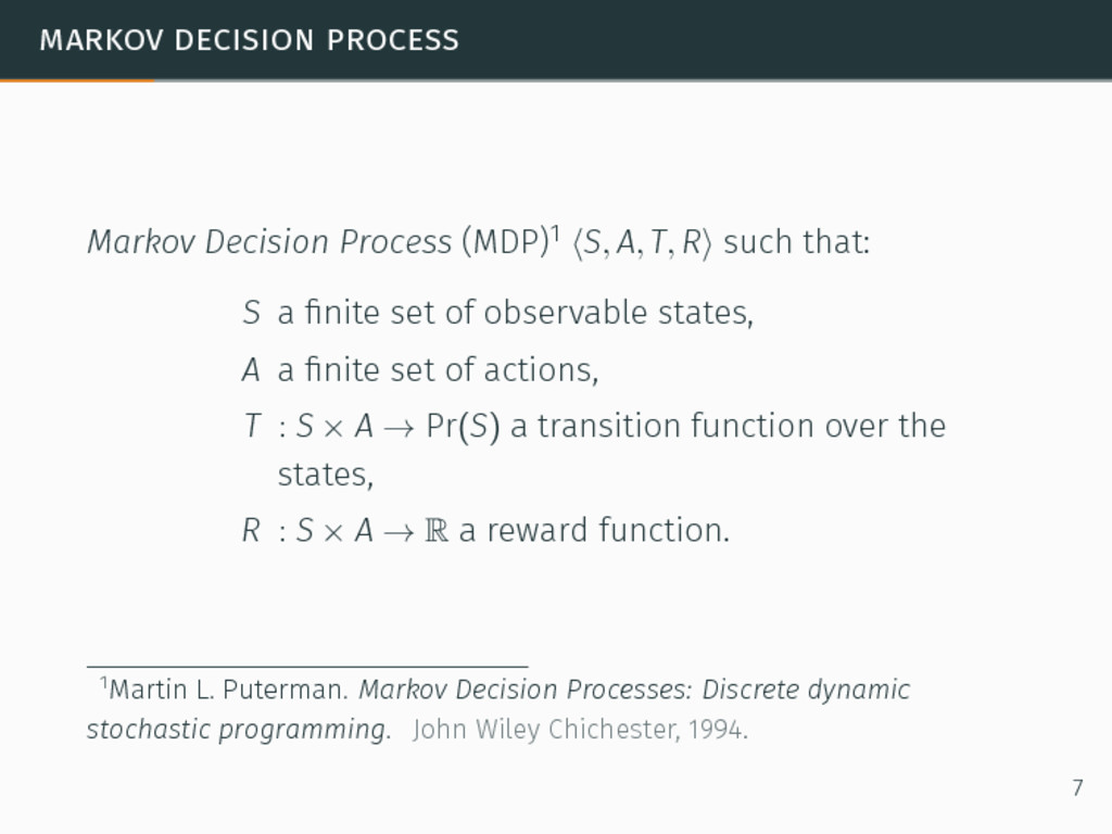
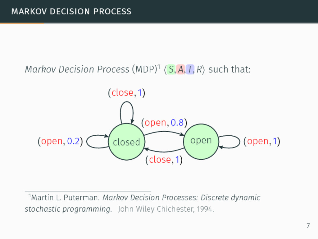
R⟩ such that: S a ﬁnite set of observable states, 1Martin L. Puterman. Markov Decision Processes: Discrete dynamic stochastic programming. John Wiley Chichester, 1994. 7

R⟩ such that: S a ﬁnite set of observable states, A a ﬁnite set of actions, 1Martin L. Puterman. Markov Decision Processes: Discrete dynamic stochastic programming. John Wiley Chichester, 1994. 7

R⟩ such that: S a ﬁnite set of observable states, A a ﬁnite set of actions, T : S × A → Pr(S) a transition function over the states, 1Martin L. Puterman. Markov Decision Processes: Discrete dynamic stochastic programming. John Wiley Chichester, 1994. 7

R⟩ such that: S a ﬁnite set of observable states, A a ﬁnite set of actions, T : S × A → Pr(S) a transition function over the states, R : S × A → R a reward function. 1Martin L. Puterman. Markov Decision Processes: Discrete dynamic stochastic programming. John Wiley Chichester, 1994. 7

markov decision process Markov Decision Process (MDP)1 ⟨ S, A,
T, R⟩ such that: closed open (open, 0.8) (close, 1) (open, 0.2) (close, 1) (open, 1) 1Martin L. Puterman. Markov Decision Processes: Discrete dynamic stochastic programming. John Wiley Chichester, 1994. 7

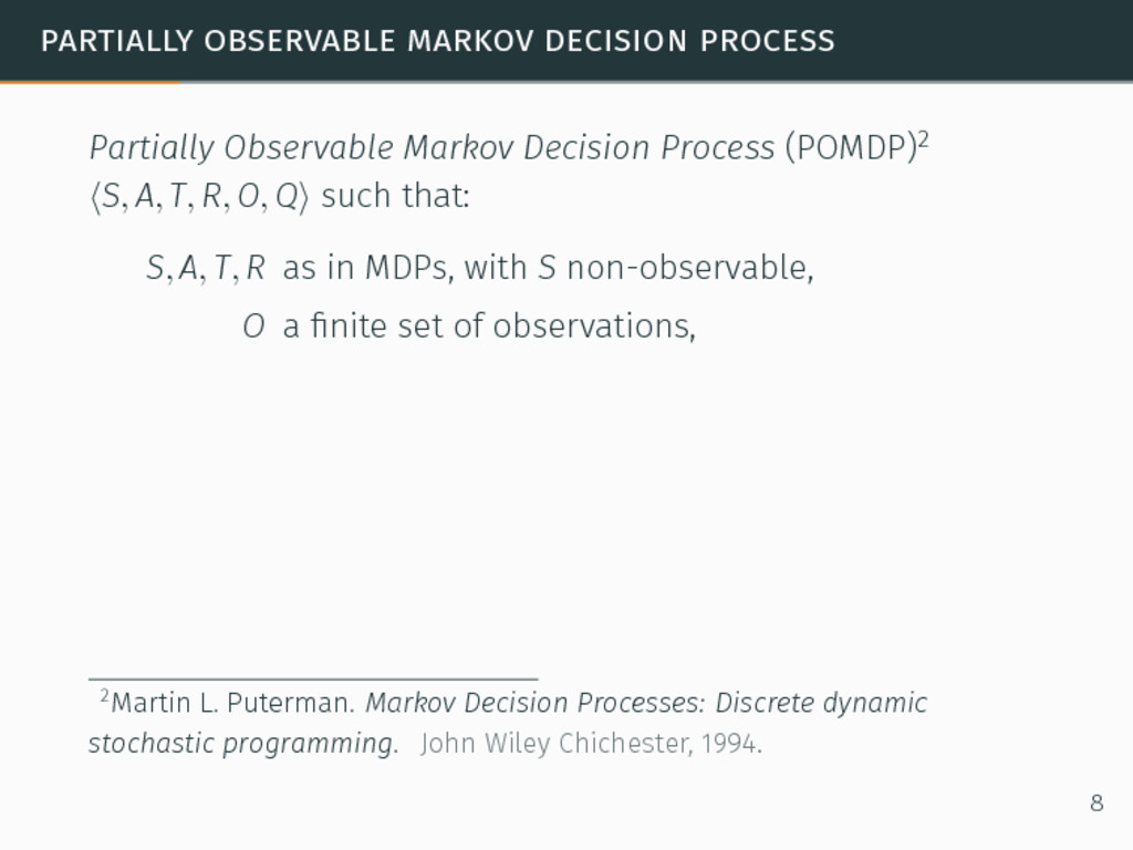
partially observable markov decision process Partially Observable Markov Decision Process
(POMDP)2 ⟨S, A, T, R, O, Q⟩ such that: 2Martin L. Puterman. Markov Decision Processes: Discrete dynamic stochastic programming. John Wiley Chichester, 1994. 8

(POMDP)2 ⟨S, A, T, R, O, Q⟩ such that: S, A, T, R as in MDPs, with S non-observable, 2Martin L. Puterman. Markov Decision Processes: Discrete dynamic stochastic programming. John Wiley Chichester, 1994. 8

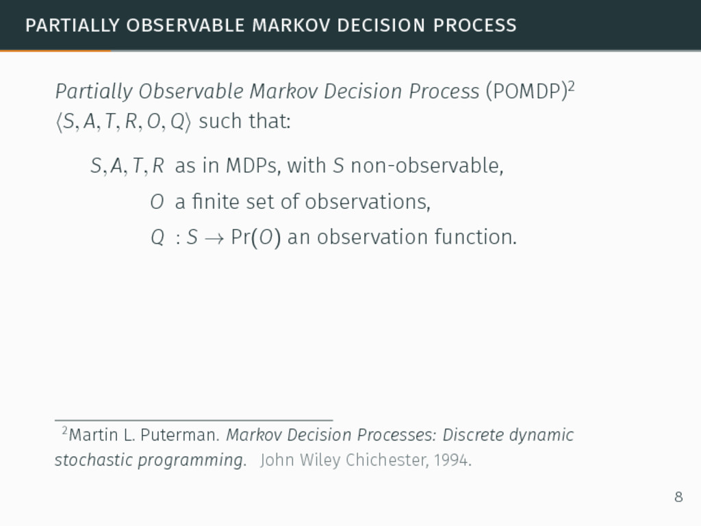
(POMDP)2 ⟨S, A, T, R, O, Q⟩ such that: S, A, T, R as in MDPs, with S non-observable, O a ﬁnite set of observations, 2Martin L. Puterman. Markov Decision Processes: Discrete dynamic stochastic programming. John Wiley Chichester, 1994. 8

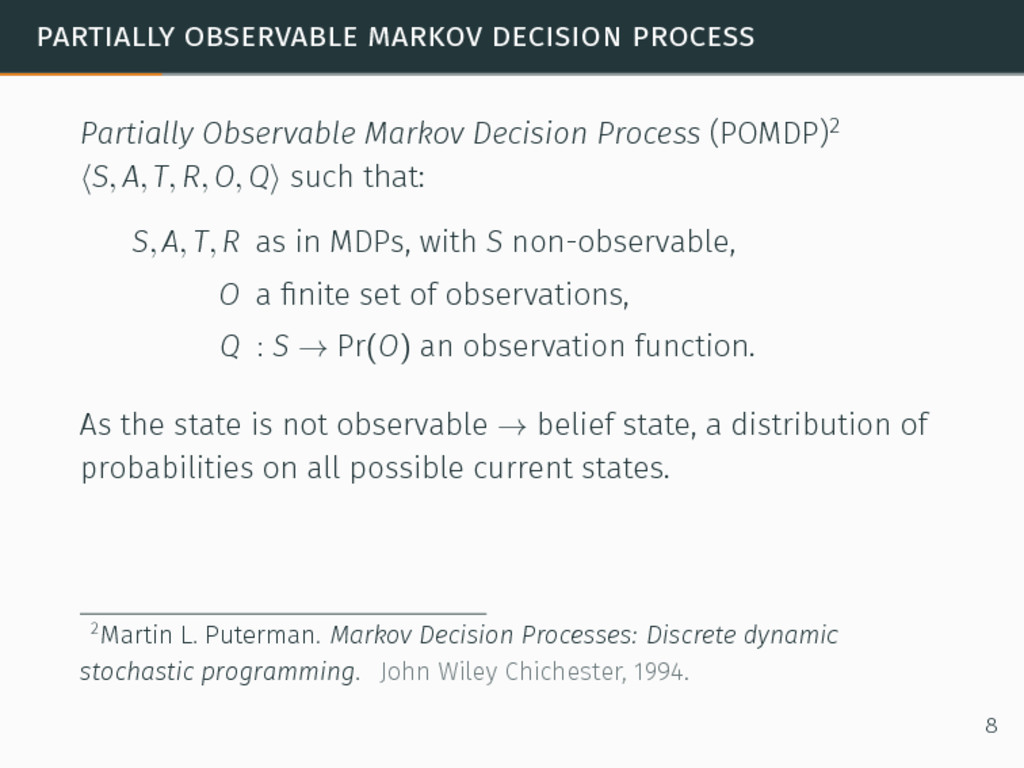
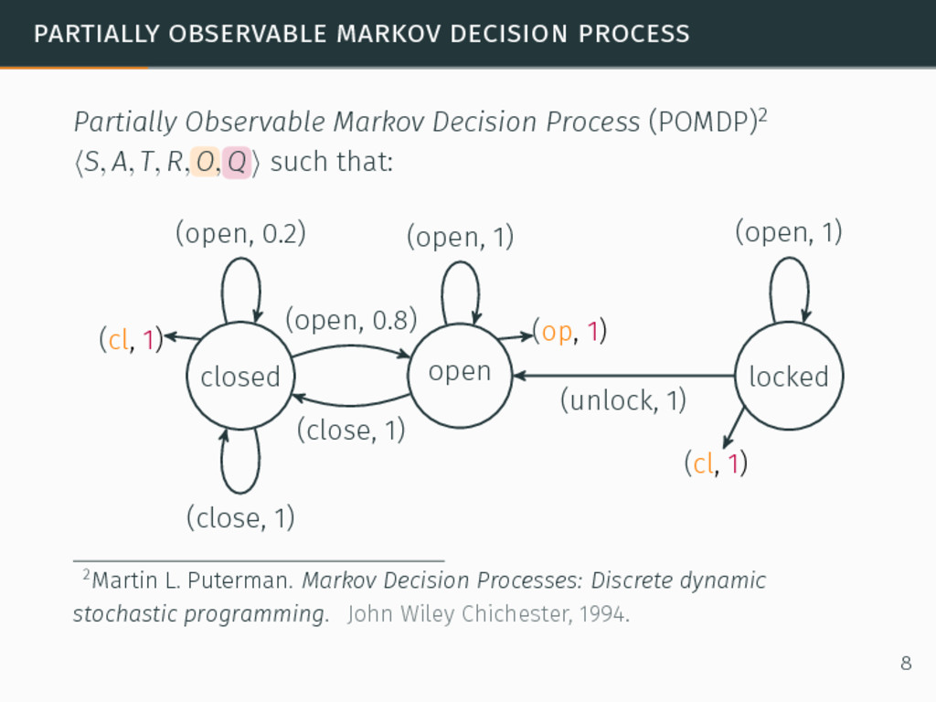
(POMDP)2 ⟨S, A, T, R, O, Q⟩ such that: S, A, T, R as in MDPs, with S non-observable, O a ﬁnite set of observations, Q : S → Pr(O) an observation function. 2Martin L. Puterman. Markov Decision Processes: Discrete dynamic stochastic programming. John Wiley Chichester, 1994. 8

(POMDP)2 ⟨S, A, T, R, O, Q⟩ such that: S, A, T, R as in MDPs, with S non-observable, O a ﬁnite set of observations, Q : S → Pr(O) an observation function. As the state is not observable → belief state, a distribution of probabilities on all possible current states. 2Martin L. Puterman. Markov Decision Processes: Discrete dynamic stochastic programming. John Wiley Chichester, 1994. 8

(POMDP)2 ⟨S, A, T, R, O, Q ⟩ such that: closed open locked (cl, 1) (op, 1) (cl, 1) (open, 0.8) (close, 1) (open, 0.2) (close, 1) (open, 1) (open, 1) (unlock, 1) 2Martin L. Puterman. Markov Decision Processes: Discrete dynamic stochastic programming. John Wiley Chichester, 1994. 8

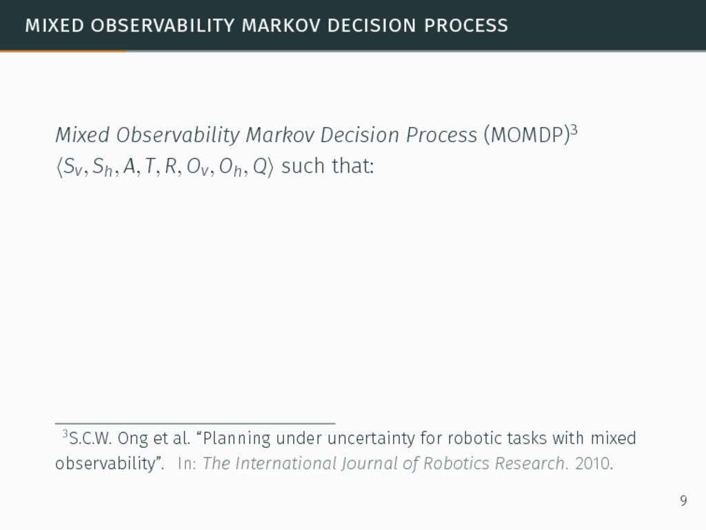
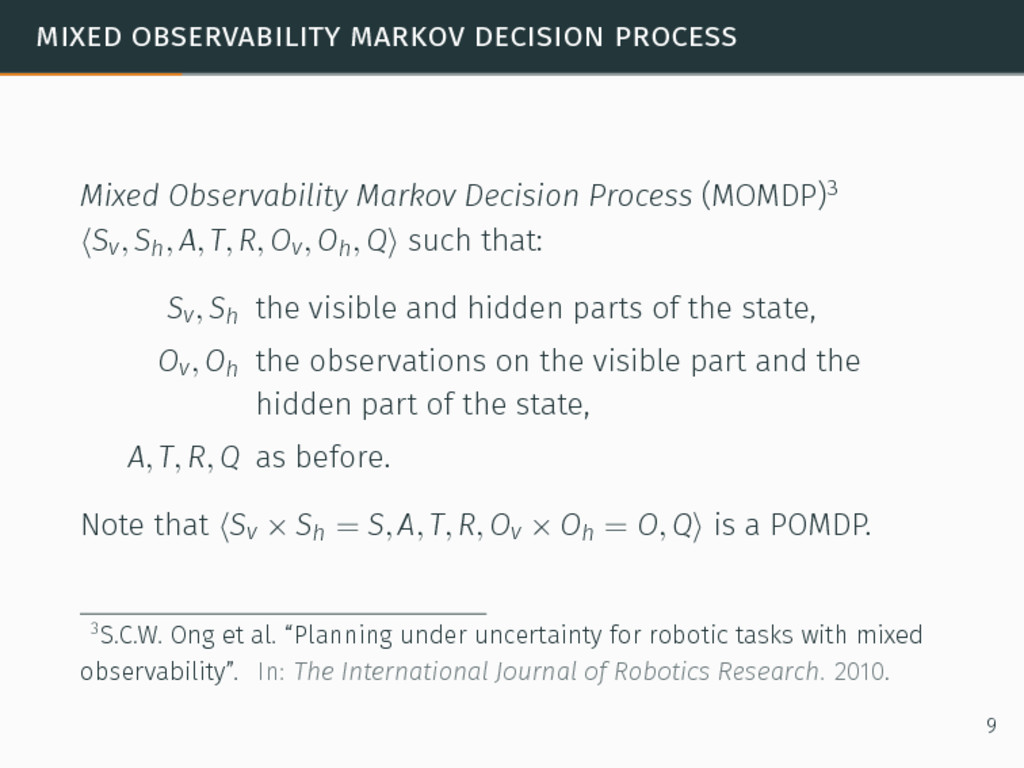
mixed observability markov decision process Mixed Observability Markov Decision Process
(MOMDP)3 ⟨Sv, Sh, A, T, R, Ov, Oh, Q⟩ such that: 3S.C.W. Ong et al. “Planning under uncertainty for robotic tasks with mixed observability”. In: The International Journal of Robotics Research. 2010. 9

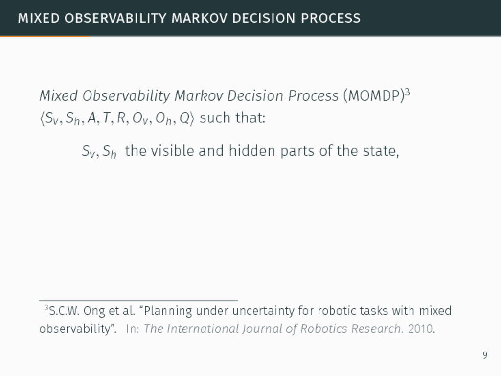
(MOMDP)3 ⟨Sv, Sh, A, T, R, Ov, Oh, Q⟩ such that: Sv, Sh the visible and hidden parts of the state, 3S.C.W. Ong et al. “Planning under uncertainty for robotic tasks with mixed observability”. In: The International Journal of Robotics Research. 2010. 9

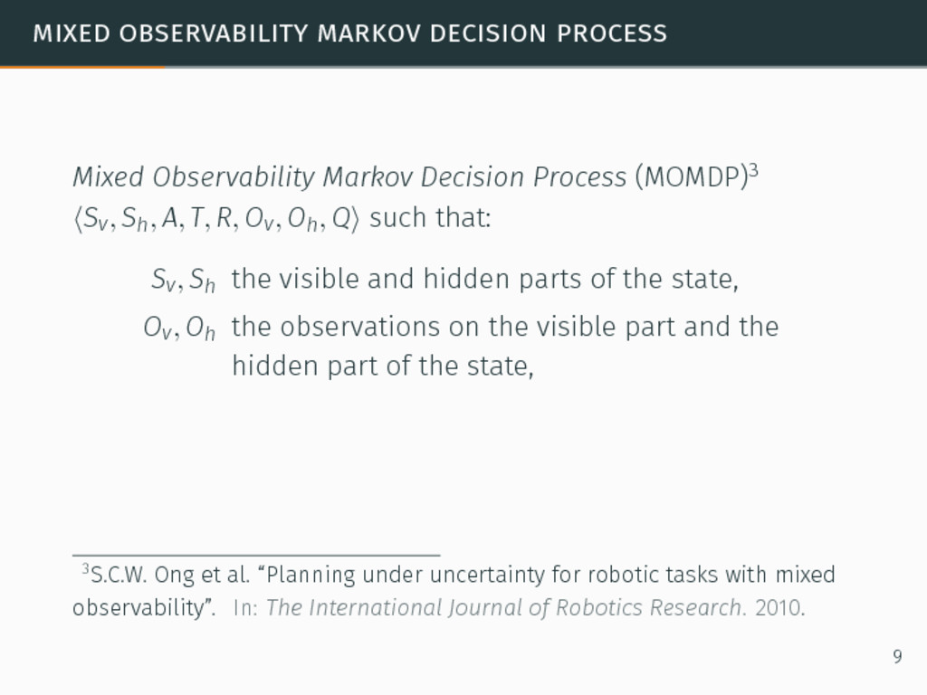
(MOMDP)3 ⟨Sv, Sh, A, T, R, Ov, Oh, Q⟩ such that: Sv, Sh the visible and hidden parts of the state, Ov, Oh the observations on the visible part and the hidden part of the state, 3S.C.W. Ong et al. “Planning under uncertainty for robotic tasks with mixed observability”. In: The International Journal of Robotics Research. 2010. 9

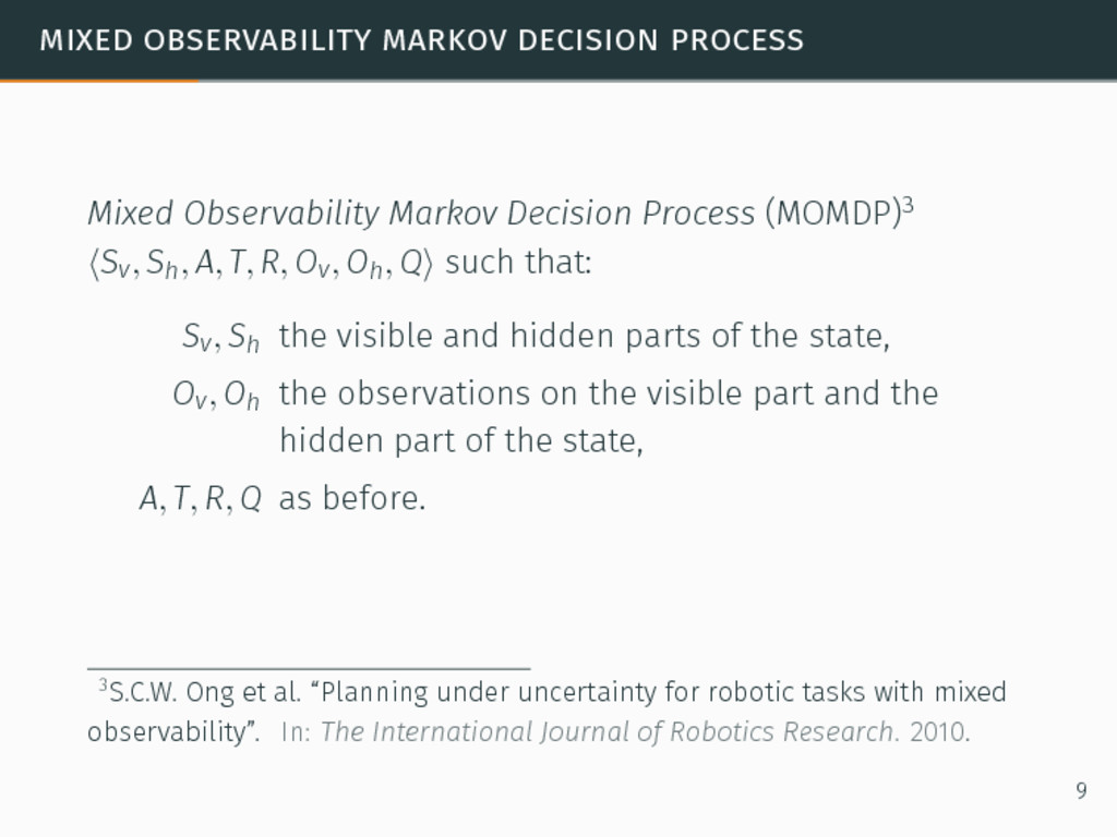
(MOMDP)3 ⟨Sv, Sh, A, T, R, Ov, Oh, Q⟩ such that: Sv, Sh the visible and hidden parts of the state, Ov, Oh the observations on the visible part and the hidden part of the state, A, T, R, Q as before. 3S.C.W. Ong et al. “Planning under uncertainty for robotic tasks with mixed observability”. In: The International Journal of Robotics Research. 2010. 9

(MOMDP)3 ⟨Sv, Sh, A, T, R, Ov, Oh, Q⟩ such that: Sv, Sh the visible and hidden parts of the state, Ov, Oh the observations on the visible part and the hidden part of the state, A, T, R, Q as before. Note that ⟨Sv × Sh = S, A, T, R, Ov × Oh = O, Q⟩ is a POMDP. 3S.C.W. Ong et al. “Planning under uncertainty for robotic tasks with mixed observability”. In: The International Journal of Robotics Research. 2010. 9

mixed observability markov decision process Let us consider, building on
the previous example, that there is the possible presence of a key on the door lock: 10

mixed observability markov decision process Let us consider, building on
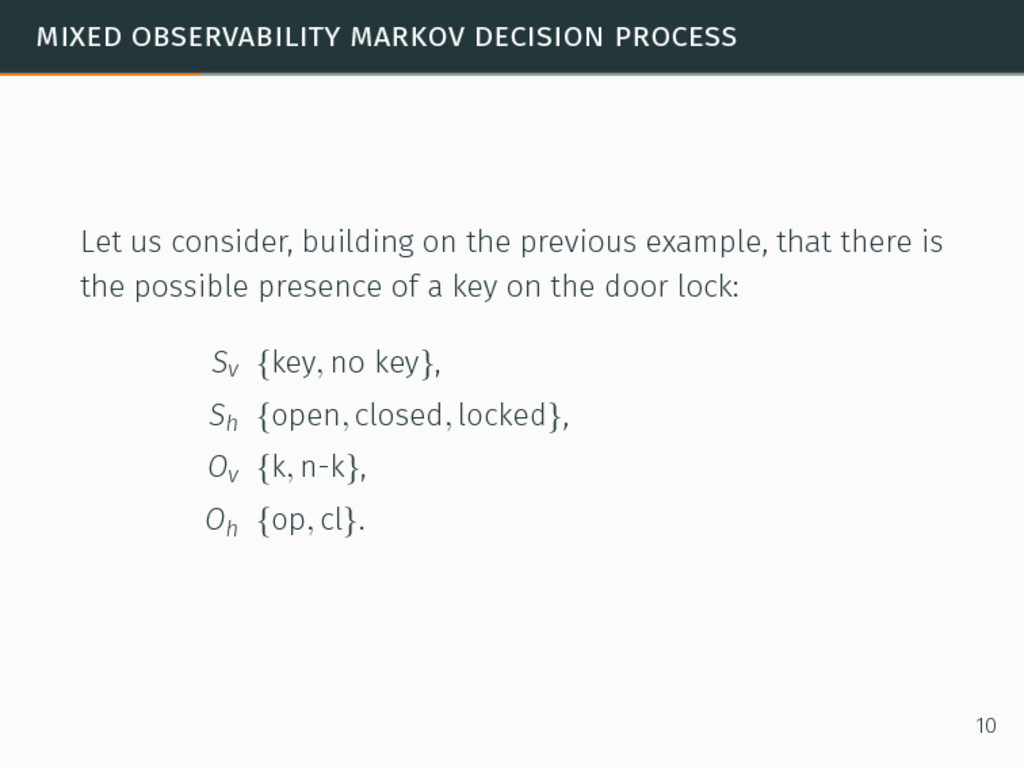
the previous example, that there is the possible presence of a key on the door lock: Sv {key, no key}, Sh {open, closed, locked}, Ov {k, n-k}, Oh {op, cl}. 10

markov decision models All those models have a common limitation:
mandatory stationarity. 11

mandatory stationarity. It is a limitation in many cases but we cannot take into account all types of non-stationarity. 11

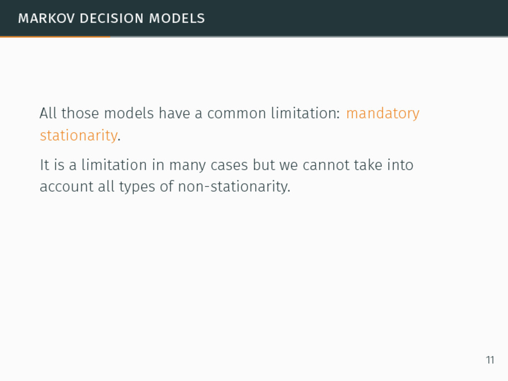
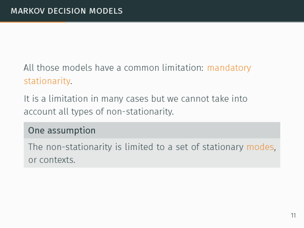
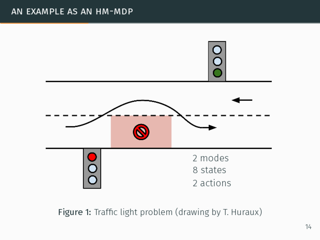
mandatory stationarity. It is a limitation in many cases but we cannot take into account all types of non-stationarity. One assumption The non-stationarity is limited to a set of stationary modes, or contexts. 11

non-stationary environments

hidden-mode markov decision process To address this subclass of problems,
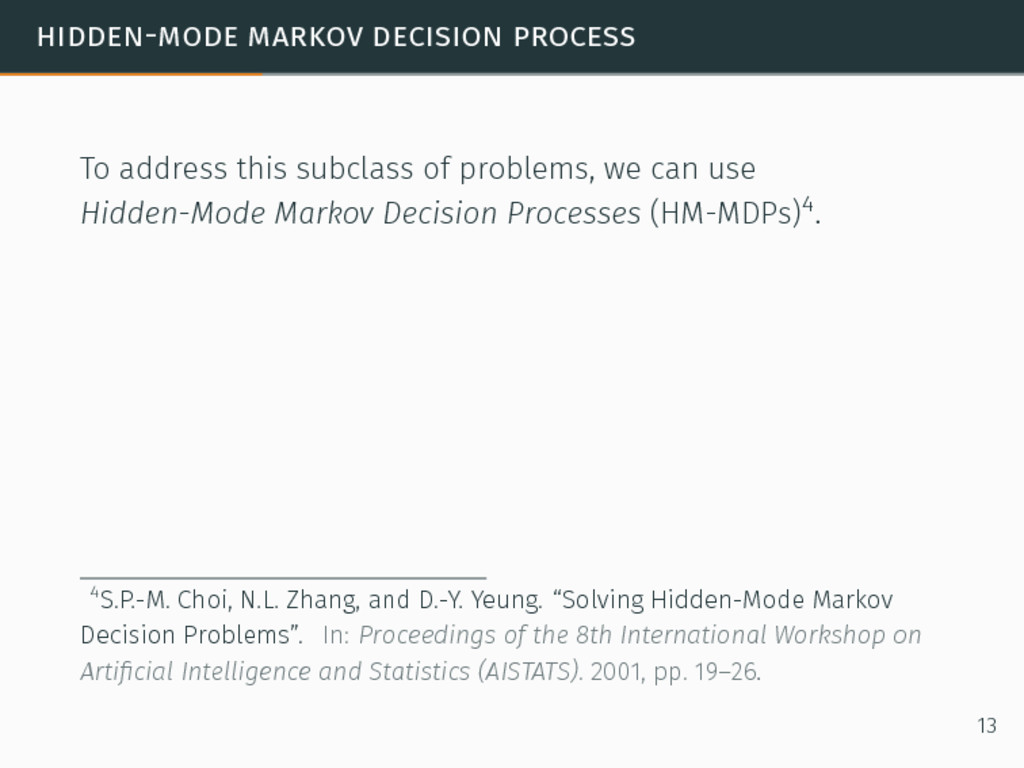
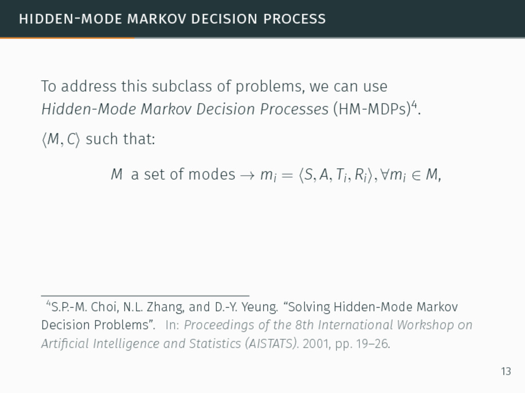
we can use Hidden-Mode Markov Decision Processes (HM-MDPs)4. 4S.P.-M. Choi, N.L. Zhang, and D.-Y. Yeung. “Solving Hidden-Mode Markov Decision Problems”. In: Proceedings of the 8th International Workshop on Artiﬁcial Intelligence and Statistics (AISTATS). 2001, pp. 19–26. 13

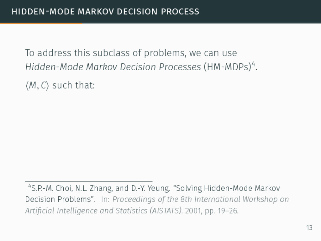
we can use Hidden-Mode Markov Decision Processes (HM-MDPs)4. ⟨M, C⟩ such that: 4S.P.-M. Choi, N.L. Zhang, and D.-Y. Yeung. “Solving Hidden-Mode Markov Decision Problems”. In: Proceedings of the 8th International Workshop on Artiﬁcial Intelligence and Statistics (AISTATS). 2001, pp. 19–26. 13

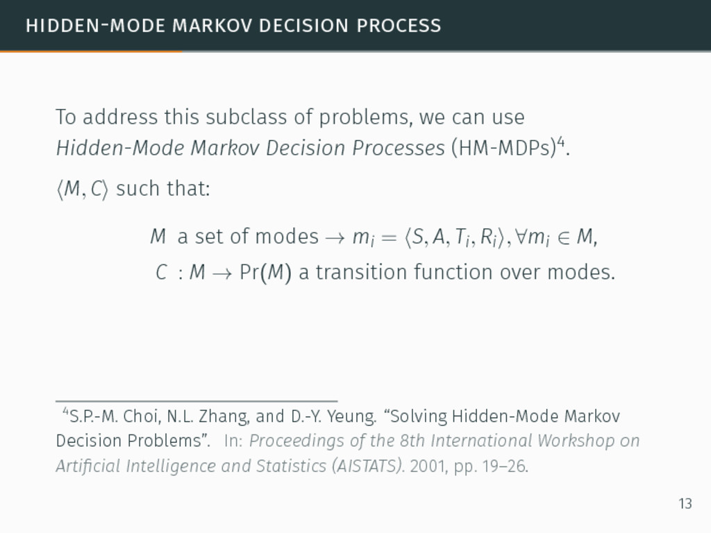
we can use Hidden-Mode Markov Decision Processes (HM-MDPs)4. ⟨M, C⟩ such that: M a set of modes → mi = ⟨S, A, Ti, Ri⟩, ∀mi ∈ M, 4S.P.-M. Choi, N.L. Zhang, and D.-Y. Yeung. “Solving Hidden-Mode Markov Decision Problems”. In: Proceedings of the 8th International Workshop on Artiﬁcial Intelligence and Statistics (AISTATS). 2001, pp. 19–26. 13

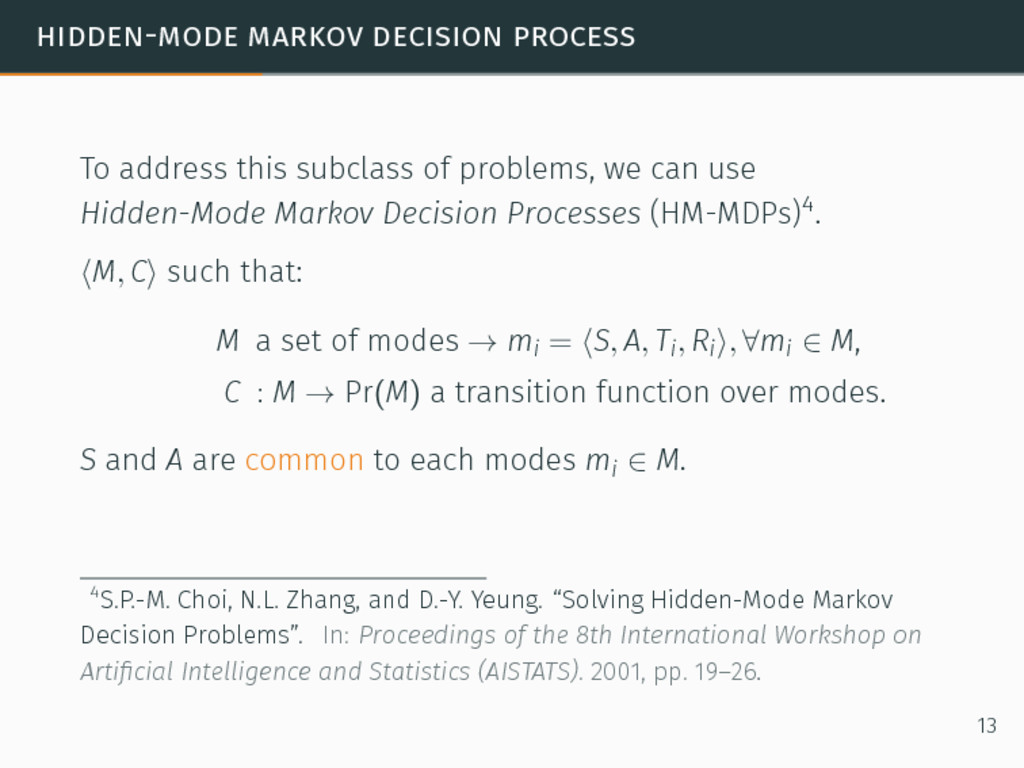
we can use Hidden-Mode Markov Decision Processes (HM-MDPs)4. ⟨M, C⟩ such that: M a set of modes → mi = ⟨S, A, Ti, Ri⟩, ∀mi ∈ M, C : M → Pr(M) a transition function over modes. 4S.P.-M. Choi, N.L. Zhang, and D.-Y. Yeung. “Solving Hidden-Mode Markov Decision Problems”. In: Proceedings of the 8th International Workshop on Artiﬁcial Intelligence and Statistics (AISTATS). 2001, pp. 19–26. 13

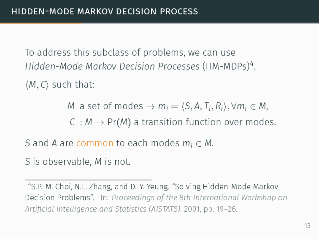
we can use Hidden-Mode Markov Decision Processes (HM-MDPs)4. ⟨M, C⟩ such that: M a set of modes → mi = ⟨S, A, Ti, Ri⟩, ∀mi ∈ M, C : M → Pr(M) a transition function over modes. S and A are common to each modes mi ∈ M. 4S.P.-M. Choi, N.L. Zhang, and D.-Y. Yeung. “Solving Hidden-Mode Markov Decision Problems”. In: Proceedings of the 8th International Workshop on Artiﬁcial Intelligence and Statistics (AISTATS). 2001, pp. 19–26. 13

we can use Hidden-Mode Markov Decision Processes (HM-MDPs)4. ⟨M, C⟩ such that: M a set of modes → mi = ⟨S, A, Ti, Ri⟩, ∀mi ∈ M, C : M → Pr(M) a transition function over modes. S and A are common to each modes mi ∈ M. S is observable, M is not. 4S.P.-M. Choi, N.L. Zhang, and D.-Y. Yeung. “Solving Hidden-Mode Markov Decision Problems”. In: Proceedings of the 8th International Workshop on Artiﬁcial Intelligence and Statistics (AISTATS). 2001, pp. 19–26. 13

an example as an hm-mdp 2 modes 8 states 2
actions Figure 1: Trafﬁc light problem (drawing by T. Huraux) 14

an example as an hm-mdp s’ s Tm1(s, a, s′)
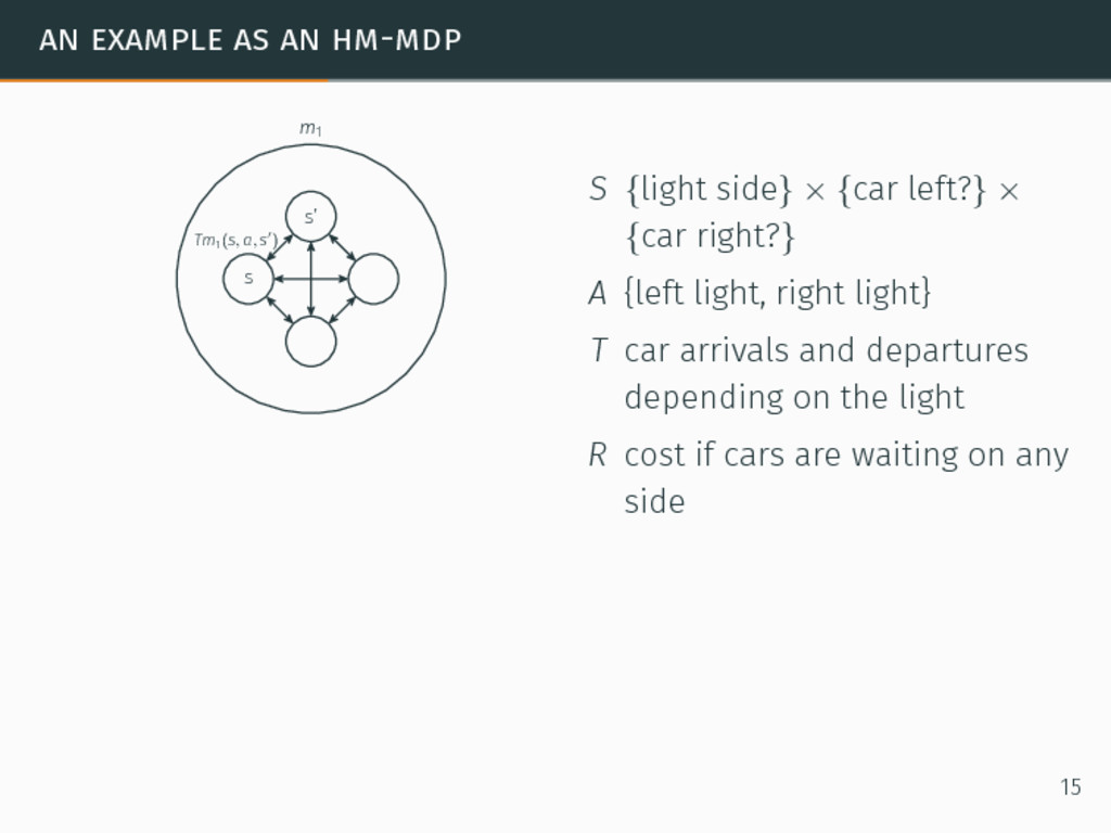
m1 S {light side} × {car left?} × {car right?} A {left light, right light} T car arrivals and departures depending on the light R cost if cars are waiting on any side 15

an example as an hm-mdp s’ s Tm1(s, a, s′)
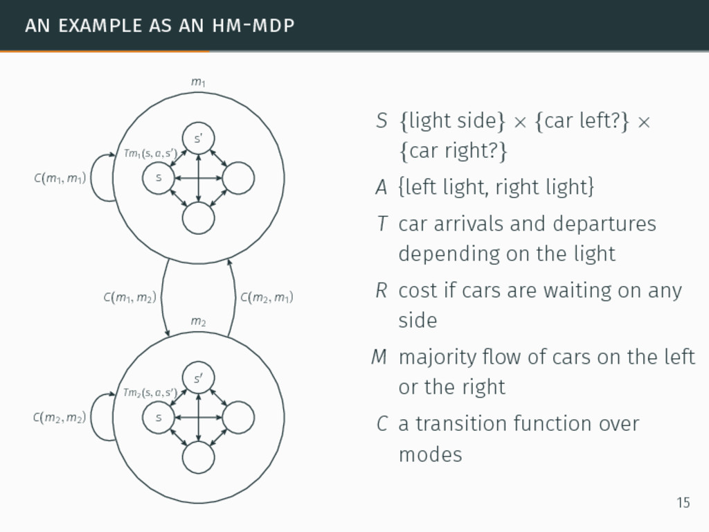
m1 s′ s Tm2(s, a, s′) m2 C(m1, m2 ) C(m2, m1 ) C(m1, m1 ) C(m2, m2 ) S {light side} × {car left?} × {car right?} A {left light, right light} T car arrivals and departures depending on the light R cost if cars are waiting on any side M majority ﬂow of cars on the left or the right C a transition function over modes 15

another limitation Each time a decision is made, the environment
may switch modes. 16

another limitation Each time a decision is made, the environment
may switch modes. In the previous example: each time the system chooses which light to turn on, the busy side may change. 16

another limitation 17

hidden-semi-markov mode markov decision process An Hidden-Semi-Markov Mode Markov Decision
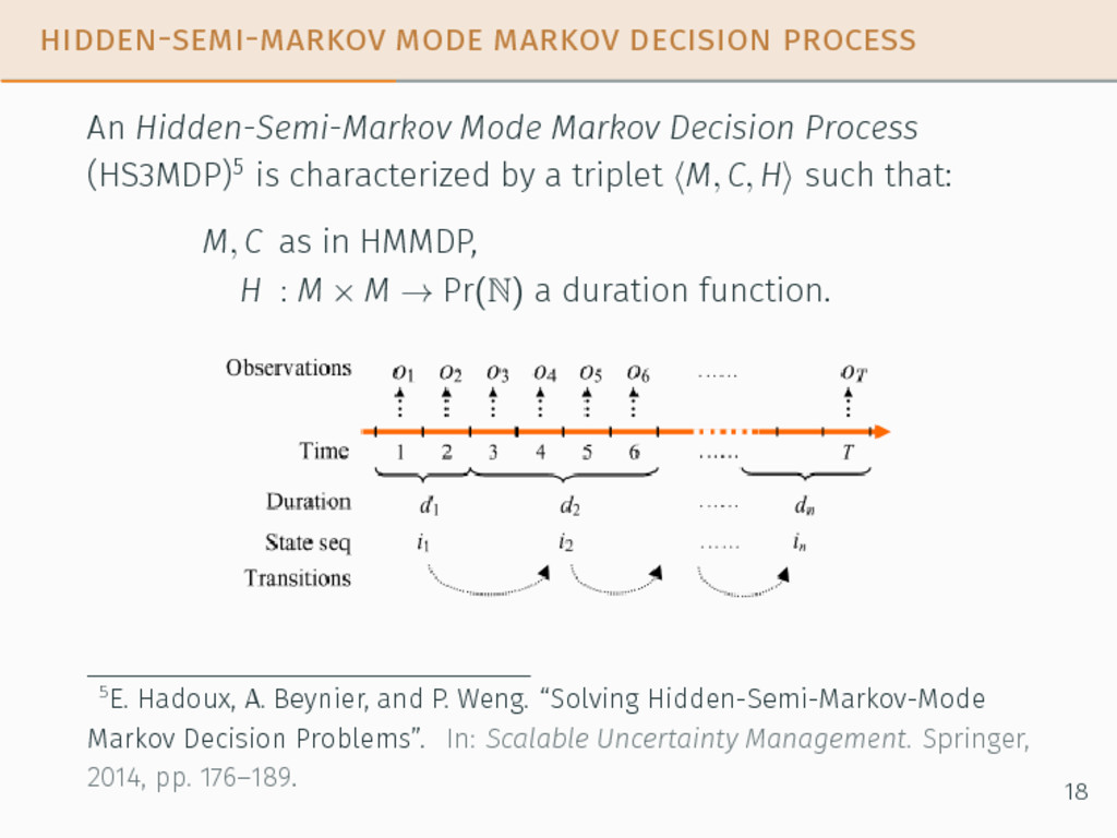
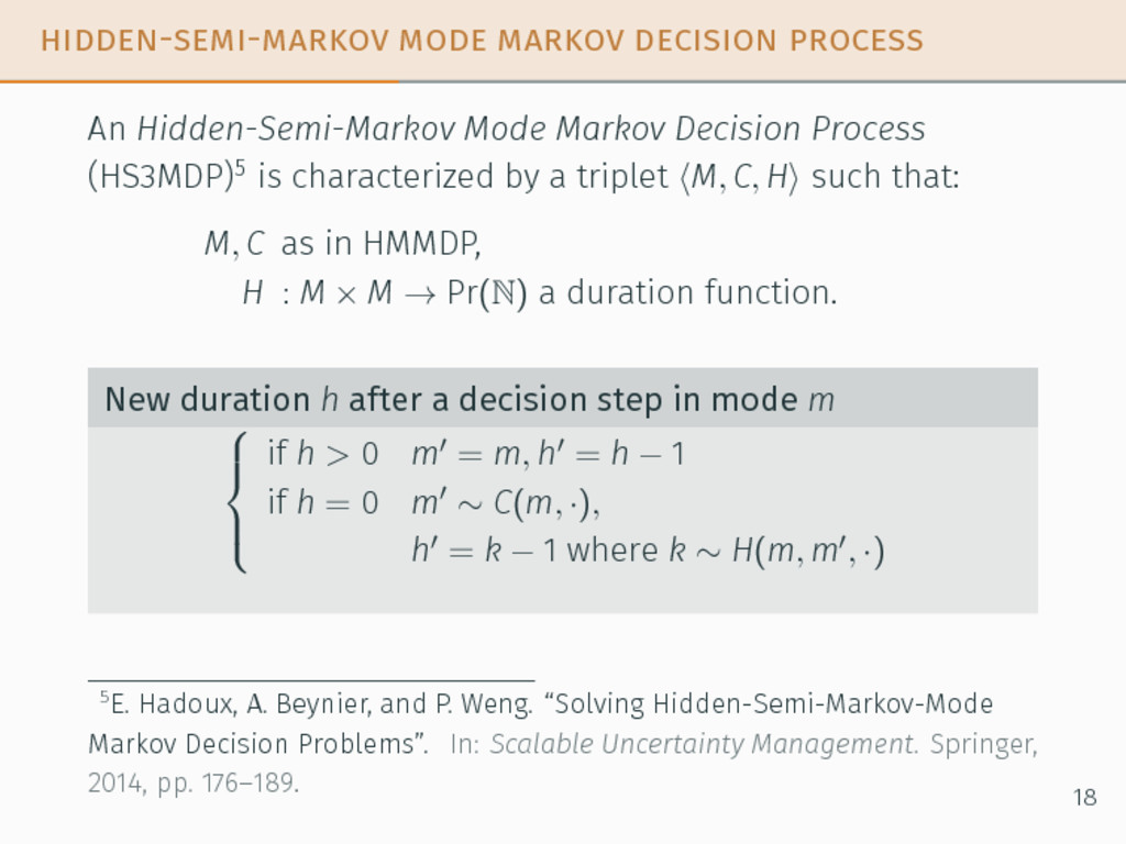
Process (HS3MDP)5 is characterized by a triplet ⟨M, C, H⟩ such that: 5E. Hadoux, A. Beynier, and P. Weng. “Solving Hidden-Semi-Markov-Mode Markov Decision Problems”. In: Scalable Uncertainty Management. Springer, 2014, pp. 176–189. 18

Process (HS3MDP)5 is characterized by a triplet ⟨M, C, H⟩ such that: M, C as in HMMDP, 5E. Hadoux, A. Beynier, and P. Weng. “Solving Hidden-Semi-Markov-Mode Markov Decision Problems”. In: Scalable Uncertainty Management. Springer, 2014, pp. 176–189. 18

Process (HS3MDP)5 is characterized by a triplet ⟨M, C, H⟩ such that: M, C as in HMMDP, H : M × M → Pr(N) a duration function. 5E. Hadoux, A. Beynier, and P. Weng. “Solving Hidden-Semi-Markov-Mode Markov Decision Problems”. In: Scalable Uncertainty Management. Springer, 2014, pp. 176–189. 18

Process (HS3MDP)5 is characterized by a triplet ⟨M, C, H⟩ such that: M, C as in HMMDP, H : M × M → Pr(N) a duration function. New duration h after a decision step in mode m      if h > 0 m′ = m, h′ = h − 1 if h = 0 m′ ∼ C(m, ·), h′ = k − 1 where k ∼ H(m, m′, ·) 5E. Hadoux, A. Beynier, and P. Weng. “Solving Hidden-Semi-Markov-Mode Markov Decision Problems”. In: Scalable Uncertainty Management. Springer, 2014, pp. 176–189. 18

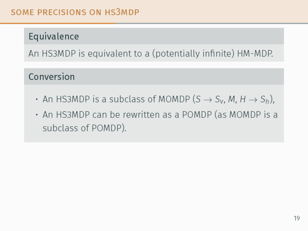
some precisions on hs3mdp Equivalence An HS3MDP is equivalent to
a (potentially inﬁnite) HM-MDP. 19

a (potentially inﬁnite) HM-MDP. Conversion • An HS3MDP is a subclass of MOMDP (S → Sv , M, H → Sh ), • An HS3MDP can be rewritten as a POMDP (as MOMDP is a subclass of POMDP). 19

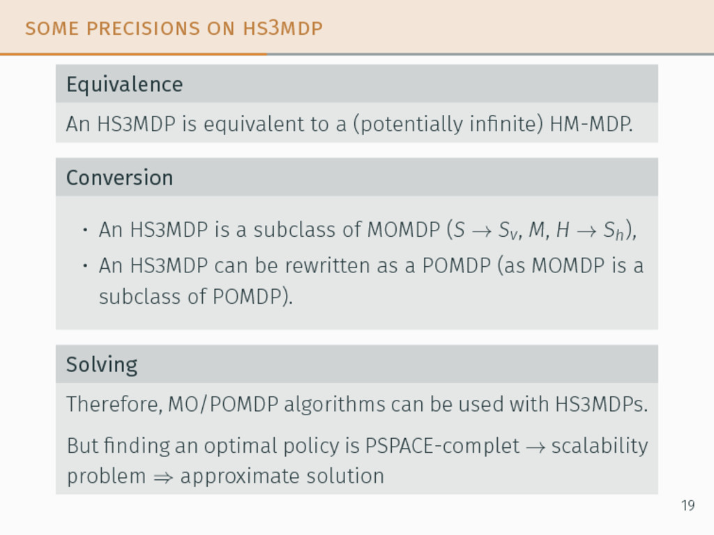
a (potentially inﬁnite) HM-MDP. Conversion • An HS3MDP is a subclass of MOMDP (S → Sv , M, H → Sh ), • An HS3MDP can be rewritten as a POMDP (as MOMDP is a subclass of POMDP). Solving Therefore, MO/POMDP algorithms can be used with HS3MDPs. But ﬁnding an optimal policy is PSPACE-complet → scalability problem ⇒ approximate solution 19

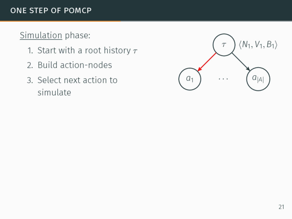
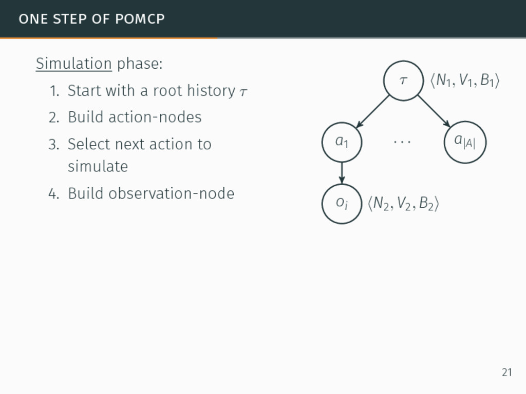
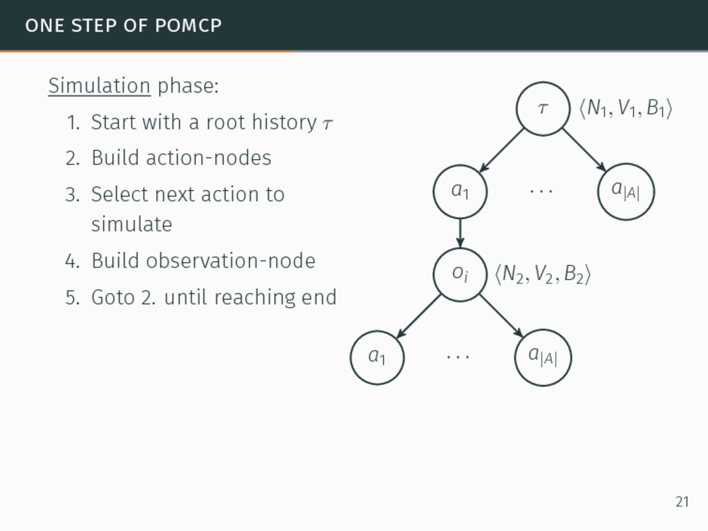
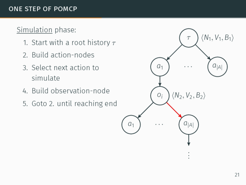
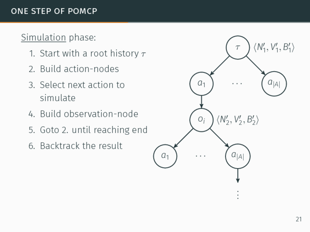
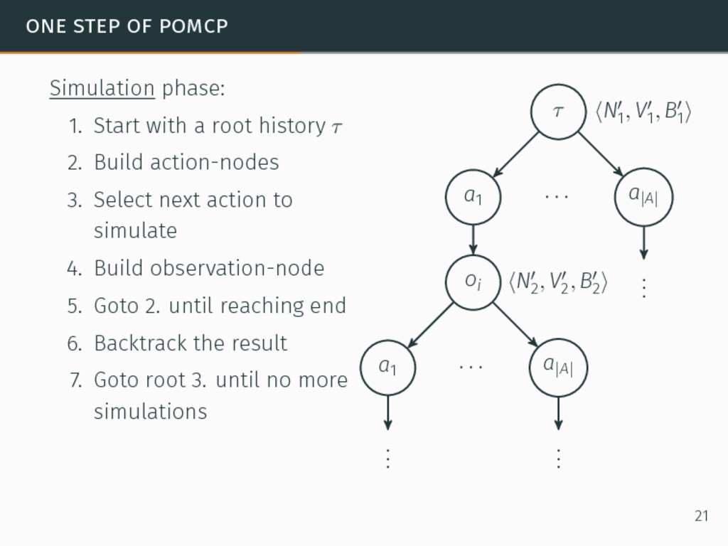
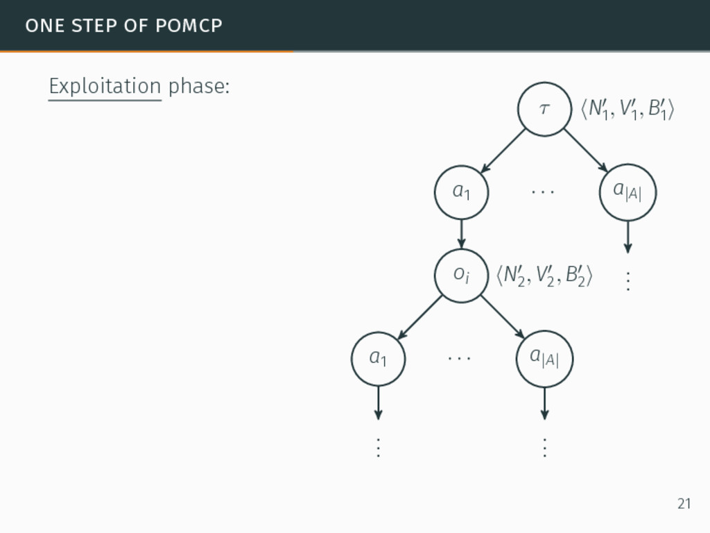
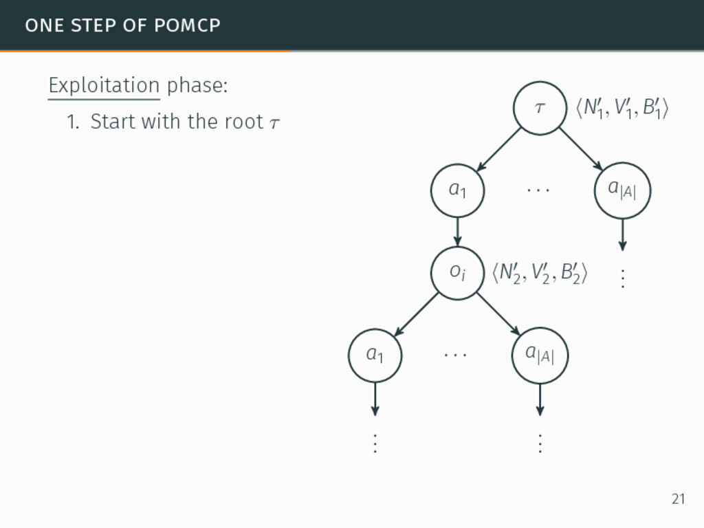
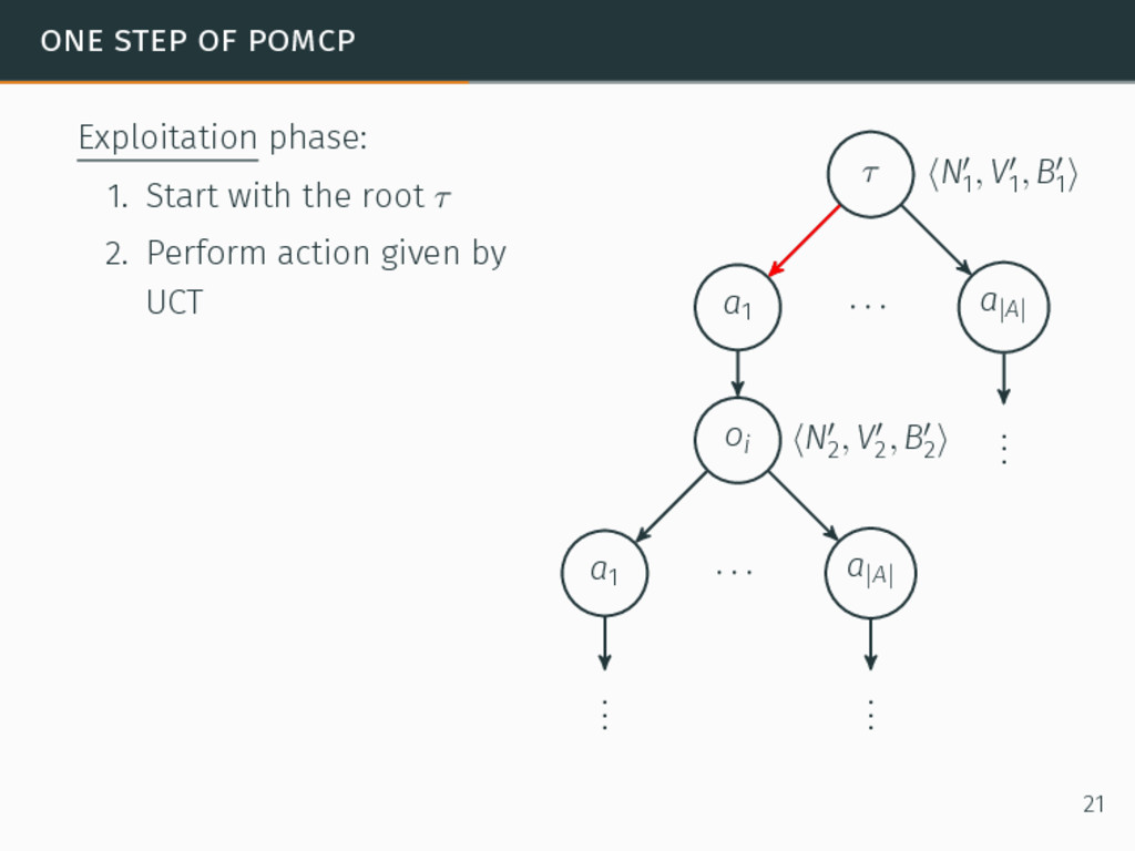
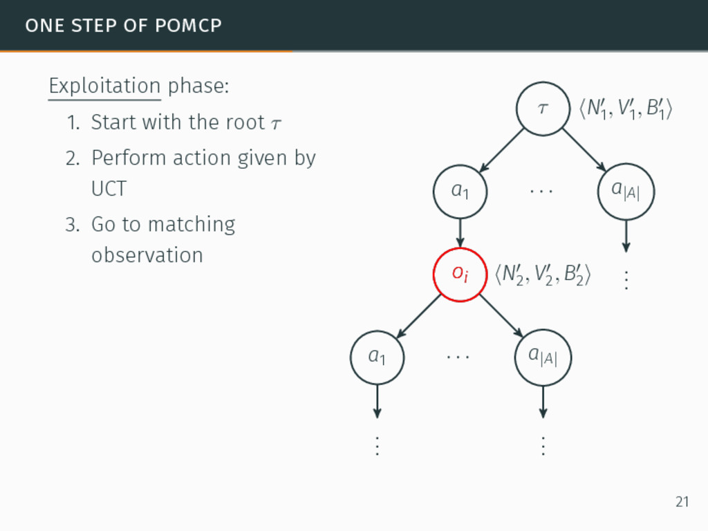
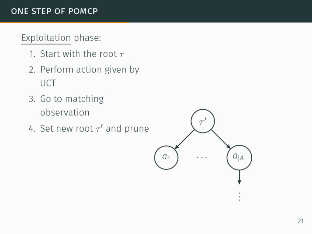
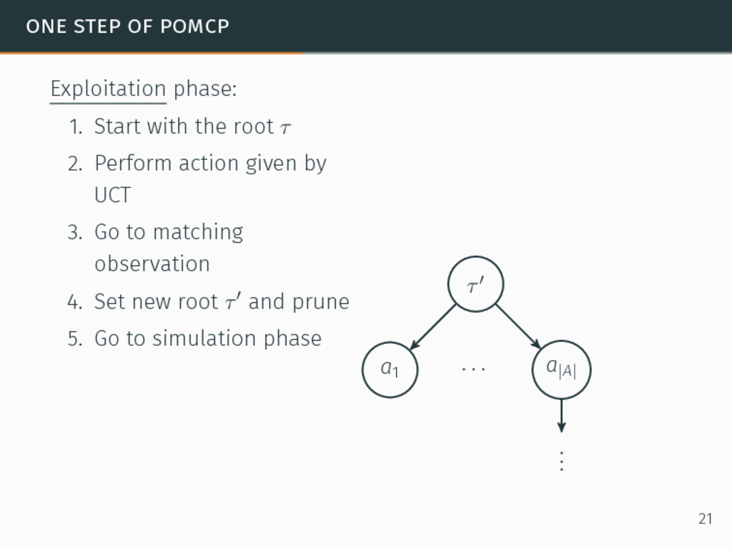
partially observable monte-carlo planning Partially Observable Monte-Carlo Planning algorithm (POMCP)6:
one of the most efﬁcient algorithms for large-sized POMDPs. POMCP characteristics 6David Silver and Joel Veness. “Monte-Carlo planning in large POMDPs”. In: Proceedings of the 24th Conference on Neural Information Processing Systems (NIPS). 2010, pp. 2164–2172. 20

one of the most efﬁcient algorithms for large-sized POMDPs. POMCP characteristics • Uses a set of particles to approximate the belief state, 6David Silver and Joel Veness. “Monte-Carlo planning in large POMDPs”. In: Proceedings of the 24th Conference on Neural Information Processing Systems (NIPS). 2010, pp. 2164–2172. 20

one of the most efﬁcient algorithms for large-sized POMDPs. POMCP characteristics • Uses a set of particles to approximate the belief state, • One particle = one state → ∞ particles = belief state, 6David Silver and Joel Veness. “Monte-Carlo planning in large POMDPs”. In: Proceedings of the 24th Conference on Neural Information Processing Systems (NIPS). 2010, pp. 2164–2172. 20

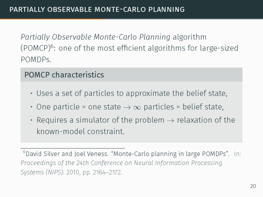
one of the most efﬁcient algorithms for large-sized POMDPs. POMCP characteristics • Uses a set of particles to approximate the belief state, • One particle = one state → ∞ particles = belief state, • Requires a simulator of the problem → relaxation of the known-model constraint. 6David Silver and Joel Veness. “Monte-Carlo planning in large POMDPs”. In: Proceedings of the 24th Conference on Neural Information Processing Systems (NIPS). 2010, pp. 2164–2172. 20

one step of pomcp Simulation phase: 1. Start with a
root history τ τ ⟨N1, V1, B1⟩ 21

root history τ 2. Build action-nodes τ ⟨N1, V1, B1⟩ · · · a1 a |A| 21

root history τ 2. Build action-nodes 3. Select next action to simulate τ ⟨N1, V1, B1⟩ · · · a1 a |A| 21

root history τ 2. Build action-nodes 3. Select next action to simulate 4. Build observation-node τ ⟨N1, V1, B1⟩ · · · a1 a |A| oi ⟨N2, V2, B2⟩ 21

root history τ 2. Build action-nodes 3. Select next action to simulate 4. Build observation-node 5. Goto 2. until reaching end τ ⟨N1, V1, B1⟩ · · · a1 a |A| oi ⟨N2, V2, B2⟩ · · · a1 a |A| 21

root history τ 2. Build action-nodes 3. Select next action to simulate 4. Build observation-node 5. Goto 2. until reaching end τ ⟨N1, V1, B1⟩ · · · a1 a |A| oi ⟨N2, V2, B2⟩ · · · a1 a |A| . . . 21

root history τ 2. Build action-nodes 3. Select next action to simulate 4. Build observation-node 5. Goto 2. until reaching end 6. Backtrack the result τ ⟨N′ 1, V′ 1, B′ 1⟩ · · · a1 a |A| oi ⟨N′ 2, V′ 2, B′ 2⟩ · · · a1 a |A| . . . 21

root history τ 2. Build action-nodes 3. Select next action to simulate 4. Build observation-node 5. Goto 2. until reaching end 6. Backtrack the result 7. Goto root 3. until no more simulations τ ⟨N′ 1, V′ 1, B′ 1⟩ · · · a1 a |A| oi ⟨N′ 2, V′ 2, B′ 2⟩ · · · a1 a |A| . . . . . . . . . 21

one step of pomcp Exploitation phase: τ ⟨N′ 1, V′
1, B′ 1⟩ · · · a1 a |A| oi ⟨N′ 2, V′ 2, B′ 2⟩ · · · a1 a |A| . . . . . . . . . 21

one step of pomcp Exploitation phase: 1. Start with the
root τ τ ⟨N′ 1, V′ 1, B′ 1⟩ · · · a1 a |A| oi ⟨N′ 2, V′ 2, B′ 2⟩ · · · a1 a |A| . . . . . . . . . 21

root τ 2. Perform action given by UCT τ ⟨N′ 1, V′ 1, B′ 1⟩ · · · a1 a |A| oi ⟨N′ 2, V′ 2, B′ 2⟩ · · · a1 a |A| . . . . . . . . . 21

root τ 2. Perform action given by UCT 3. Go to matching observation τ ⟨N′ 1, V′ 1, B′ 1⟩ · · · a1 a |A| oi ⟨N′ 2, V′ 2, B′ 2⟩ oi · · · a1 a |A| . . . . . . . . . 21

root τ 2. Perform action given by UCT 3. Go to matching observation 4. Set new root τ′ and prune τ′ · · · a1 a |A| . . . 21

root τ 2. Perform action given by UCT 3. Go to matching observation 4. Set new root τ′ and prune 5. Go to simulation phase τ′ · · · a1 a |A| . . . 21

more limitations When the size of the model is too
large → particle deprivation We can add more particles → requires more computing time 22

using the structure of hs3mdp Fortunately, HS3MDPs are structured POMDPs.
We deﬁned two adaptations of POMCP for HS3MDPs: 23

We deﬁned two adaptations of POMCP for HS3MDPs: 1. Adaptation to the structure 23

We deﬁned two adaptations of POMCP for HS3MDPs: 1. Adaptation to the structure 2. Exact representation of the belief state 23

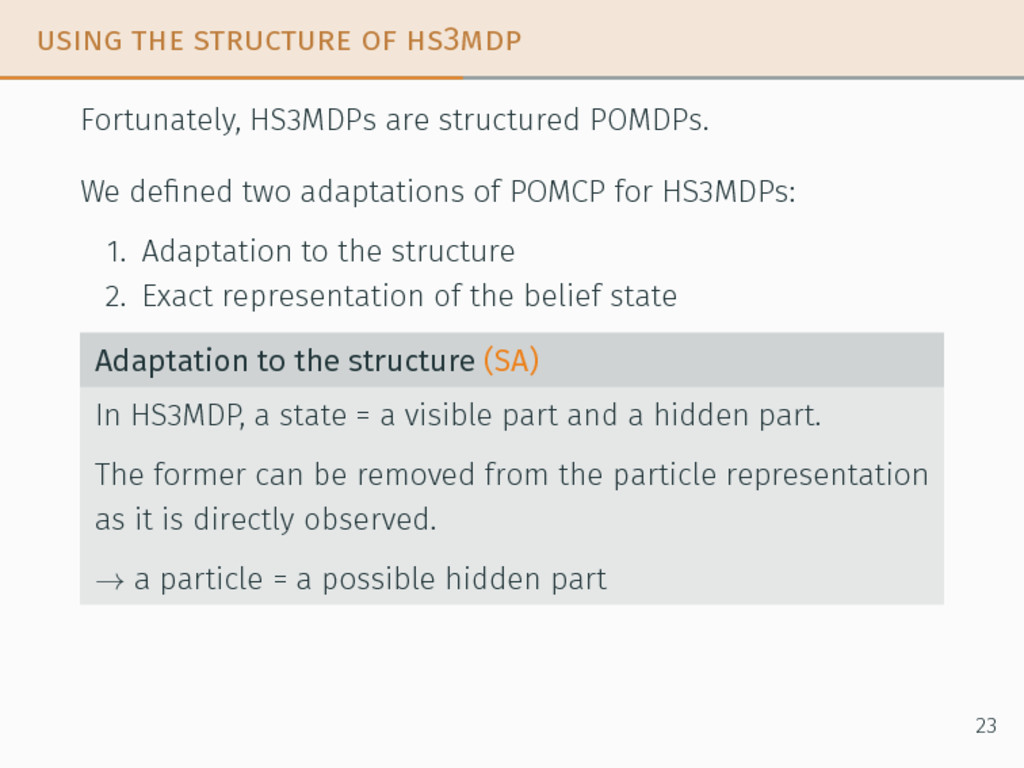
We deﬁned two adaptations of POMCP for HS3MDPs: 1. Adaptation to the structure 2. Exact representation of the belief state Adaptation to the structure (SA) In HS3MDP, a state = a visible part and a hidden part. The former can be removed from the particle representation as it is directly observed. → a particle = a possible hidden part 23

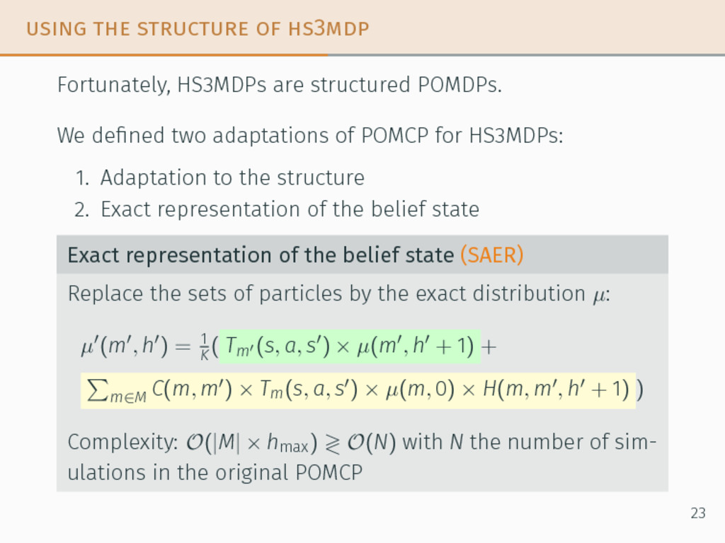
We deﬁned two adaptations of POMCP for HS3MDPs: 1. Adaptation to the structure 2. Exact representation of the belief state Exact representation of the belief state (SAER) Replace the sets of particles by the exact distribution µ: µ′(m′, h′) = 1 K ( Tm′ (s, a, s′) × µ(m′, h′ + 1) + ∑ m∈M C(m, m′) × Tm(s, a, s′) × µ(m, 0) × H(m, m′, h′ + 1) ) Complexity: O(|M| × hmax) ≷ O(N) with N the number of simulations in the original POMCP 23

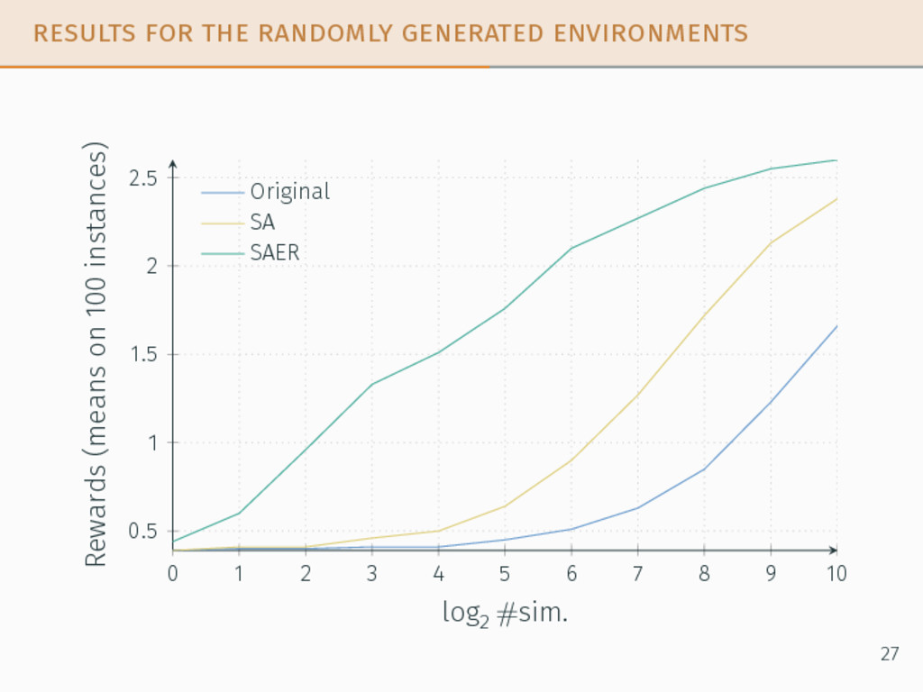
experiments We tested our method on 4 problems, with 3
taken from the literature. We compared the performances of: • the original POMCP algorithm, • our adaptations SA and SAER, • the optimal policy when it can be computed 24

results for the traffic light problem Simulations Original SA SAER
Optimal 1 -3,42 0.0% 0.0% 38.5% 2 -2,86 3.0% 4.0% 26.5% 4 -2,80 8.1% 8.8% 25.0% 8 -2,68 6.0% 9.4% 21.7% 16 -2,60 8.0% 8.0% 19.2% 32 -2,45 5.3% 6.9% 14.3% · · · 1024 -2,31 5.1% 7.0% 9.3% 25

randomly generated environments We can control the number of states,
actions and modes and the transition functions. Too big to be optimally solved. 26

results for the randomly generated environments 0 1 2 3
4 5 6 7 8 9 10 0.5 1 1.5 2 2.5 log 2 #sim. Rewards (means on 100 instances) Original SA SAER 27

conclusion on hs3mdps We proposed in this work: 28

conclusion on hs3mdps We proposed in this work: • A
new model able to represent in a more realistic way non-stationary decision-making problems (HS3MDP), 28

conclusion on hs3mdps We proposed in this work: • A
new model able to represent in a more realistic way non-stationary decision-making problems (HS3MDP), • Adaptations of POMCP to tackle large-size problems, outperforming it. 28

learning the model We also proposed a method to learn
a subclass of those problems called RLCD with SCD7. 7Emmanuel Hadoux, Aurélie Beynier, and Paul Weng. “Sequential Decision-Making under Non-stationary Environments via Sequential Change-point Detection”. In: First International Workshop on Learning over Multiple Contexts (LMCE) @ ECML. 2014. 29

learning the model We also proposed a method to learn
a subclass of those problems called RLCD with SCD7. This method is able to learn a part of the dynamics, without requiring to know the number of modes a priori. 7Emmanuel Hadoux, Aurélie Beynier, and Paul Weng. “Sequential Decision-Making under Non-stationary Environments via Sequential Change-point Detection”. In: First International Workshop on Learning over Multiple Contexts (LMCE) @ ECML. 2014. 29

strategic argumentation problems

strategic argumentation problems Few works address the problem of decision-making
in argumentation. 8Phan Minh Dung. “On the Acceptability of Arguments and its Fundamental Role in Nonmonotonic Reasoning, Logic Programming and n-Person Games”. In: Artiﬁcial Intelligence 77.2 (1995), pp. 321–358. 31

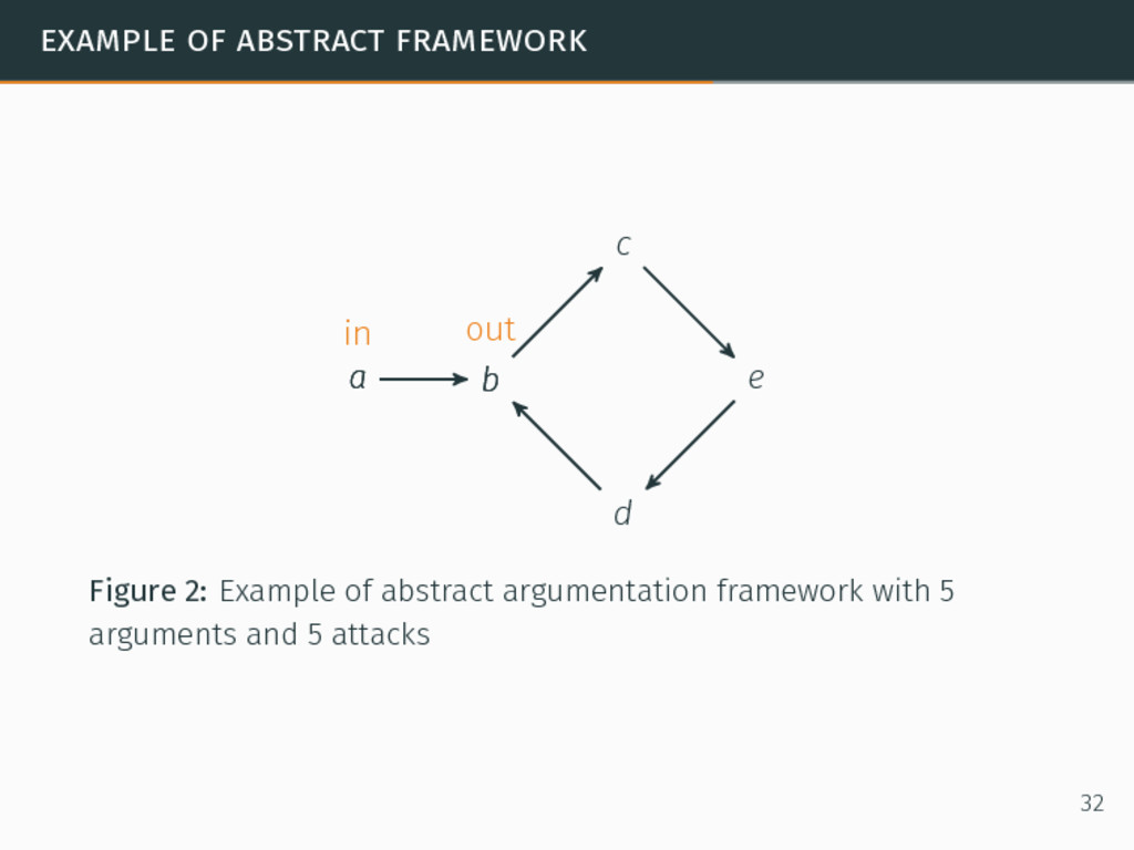
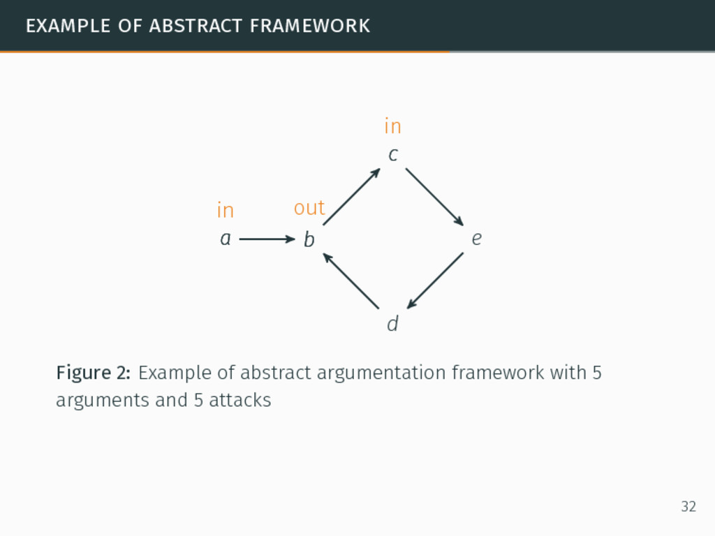
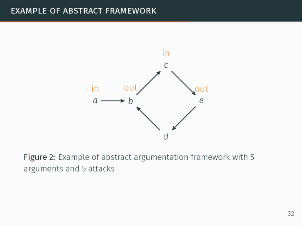
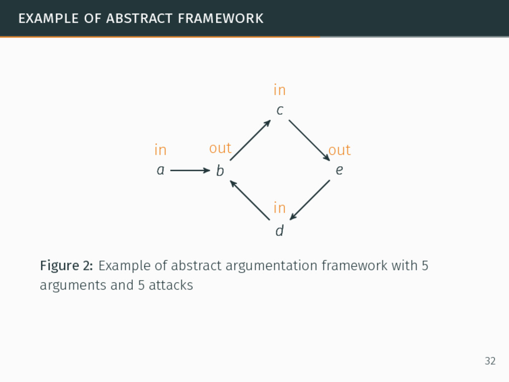
in argumentation. In abstract argumentation, agents exchange arguments and use attacks as relations between the arguments. 8Phan Minh Dung. “On the Acceptability of Arguments and its Fundamental Role in Nonmonotonic Reasoning, Logic Programming and n-Person Games”. In: Artiﬁcial Intelligence 77.2 (1995), pp. 321–358. 31

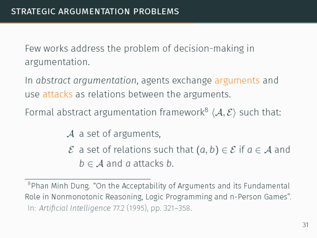
in argumentation. In abstract argumentation, agents exchange arguments and use attacks as relations between the arguments. Formal abstract argumentation framework8 ⟨A, E⟩ such that: 8Phan Minh Dung. “On the Acceptability of Arguments and its Fundamental Role in Nonmonotonic Reasoning, Logic Programming and n-Person Games”. In: Artiﬁcial Intelligence 77.2 (1995), pp. 321–358. 31

in argumentation. In abstract argumentation, agents exchange arguments and use attacks as relations between the arguments. Formal abstract argumentation framework8 ⟨A, E⟩ such that: A a set of arguments, 8Phan Minh Dung. “On the Acceptability of Arguments and its Fundamental Role in Nonmonotonic Reasoning, Logic Programming and n-Person Games”. In: Artiﬁcial Intelligence 77.2 (1995), pp. 321–358. 31

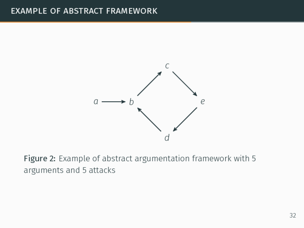
in argumentation. In abstract argumentation, agents exchange arguments and use attacks as relations between the arguments. Formal abstract argumentation framework8 ⟨A, E⟩ such that: A a set of arguments, E a set of relations such that (a, b) ∈ E if a ∈ A and b ∈ A and a attacks b. 8Phan Minh Dung. “On the Acceptability of Arguments and its Fundamental Role in Nonmonotonic Reasoning, Logic Programming and n-Person Games”. In: Artiﬁcial Intelligence 77.2 (1995), pp. 321–358. 31

example of abstract framework a b c d e Figure
2: Example of abstract argumentation framework with 5 arguments and 5 attacks 32

example of abstract framework a a in b c d
e Figure 2: Example of abstract argumentation framework with 5 arguments and 5 attacks 32

example of abstract framework a a in b b out
c d e Figure 2: Example of abstract argumentation framework with 5 arguments and 5 attacks 32

c c in d e Figure 2: Example of abstract argumentation framework with 5 arguments and 5 attacks 32

c c in d e e out Figure 2: Example of abstract argumentation framework with 5 arguments and 5 attacks 32

c c in d d in e e out Figure 2: Example of abstract argumentation framework with 5 arguments and 5 attacks 32

decision-making in argumentation More recently: argumentation framework with probabilistic strategies9
against stochastic opponents. 9Anthony Hunter. “Probabilistic Strategies in Dialogical Argumentation”. In: International Conference on Scalable Uncertainty Management (SUM) LNCS volume 8720. 2014. 33

against stochastic opponents. Agents play a turn-based game → argumentative dialogue 9Anthony Hunter. “Probabilistic Strategies in Dialogical Argumentation”. In: International Conference on Scalable Uncertainty Management (SUM) LNCS volume 8720. 2014. 33

against stochastic opponents. Agents play a turn-based game → argumentative dialogue Uses executable logic to represent the actions of an agent in the debate. 9Anthony Hunter. “Probabilistic Strategies in Dialogical Argumentation”. In: International Conference on Scalable Uncertainty Management (SUM) LNCS volume 8720. 2014. 33

argumentation framework with probabilistic strategies Each agent has a private
state. 34

state. The problem has a public space. 34

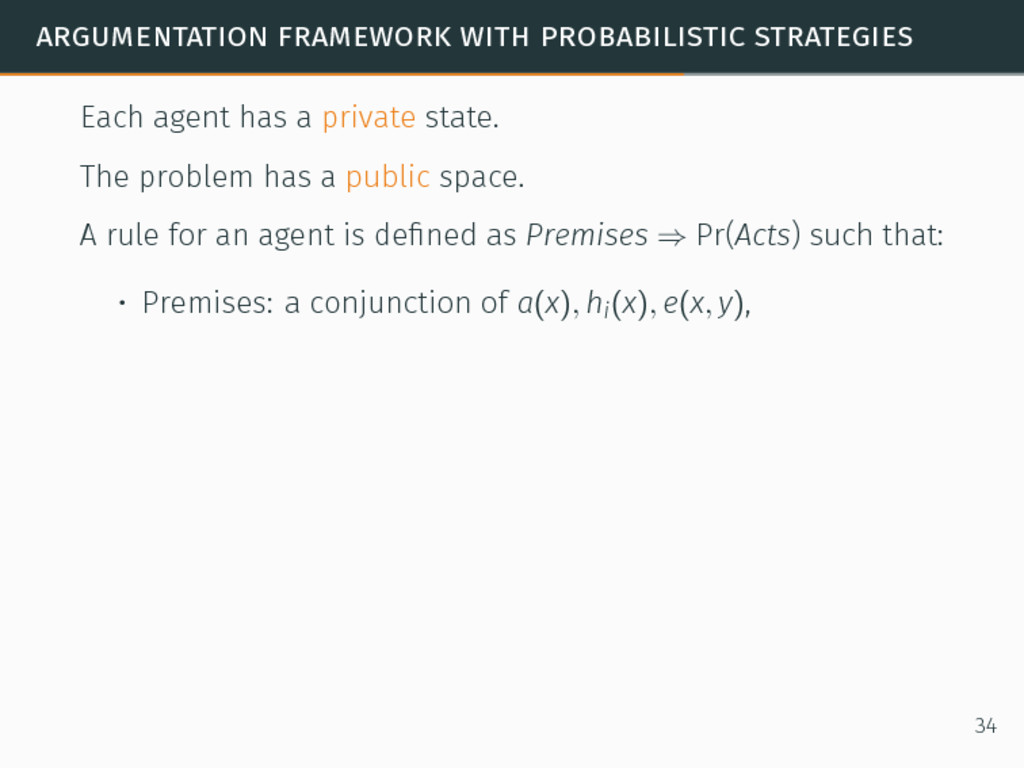
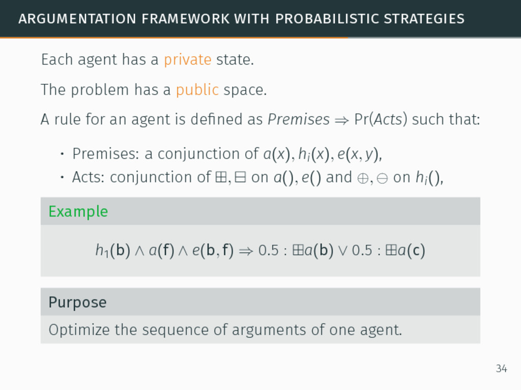
state. The problem has a public space. A rule for an agent is deﬁned as Premises ⇒ Pr(Acts) such that: • Premises: a conjunction of a(x), hi(x), e(x, y), 34

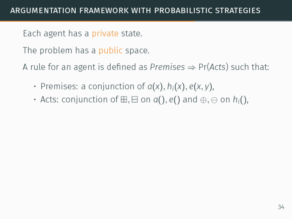
state. The problem has a public space. A rule for an agent is deﬁned as Premises ⇒ Pr(Acts) such that: • Premises: a conjunction of a(x), hi(x), e(x, y), • Acts: conjunction of ⊞, ⊟ on a(), e() and ⊕, ⊖ on hi(), 34

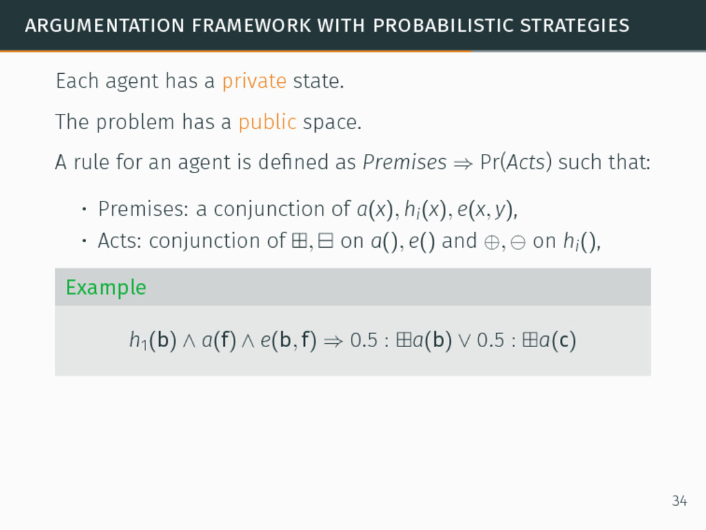
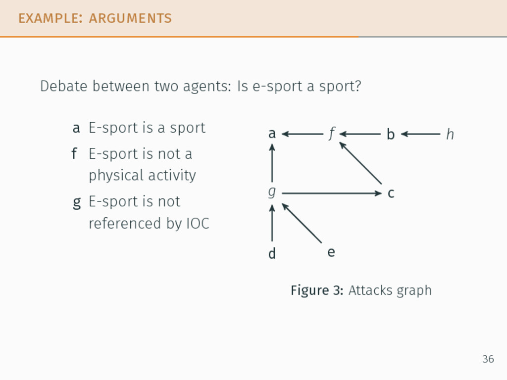
state. The problem has a public space. A rule for an agent is deﬁned as Premises ⇒ Pr(Acts) such that: • Premises: a conjunction of a(x), hi(x), e(x, y), • Acts: conjunction of ⊞, ⊟ on a(), e() and ⊕, ⊖ on hi(), Example h1(b) ∧ a(f) ∧ e(b, f) ⇒ 0.5 : ⊞a(b) ∨ 0.5 : ⊞a(c) 34

state. The problem has a public space. A rule for an agent is deﬁned as Premises ⇒ Pr(Acts) such that: • Premises: a conjunction of a(x), hi(x), e(x, y), • Acts: conjunction of ⊞, ⊟ on a(), e() and ⊕, ⊖ on hi(), Example h1(b) ∧ a(f) ∧ e(b, f) ⇒ 0.5 : ⊞a(b) ∨ 0.5 : ⊞a(c) Purpose Optimize the sequence of arguments of one agent. 34

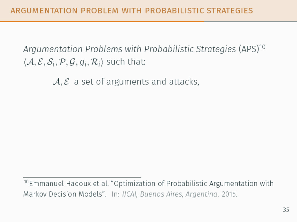
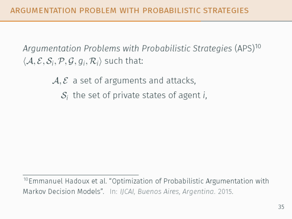
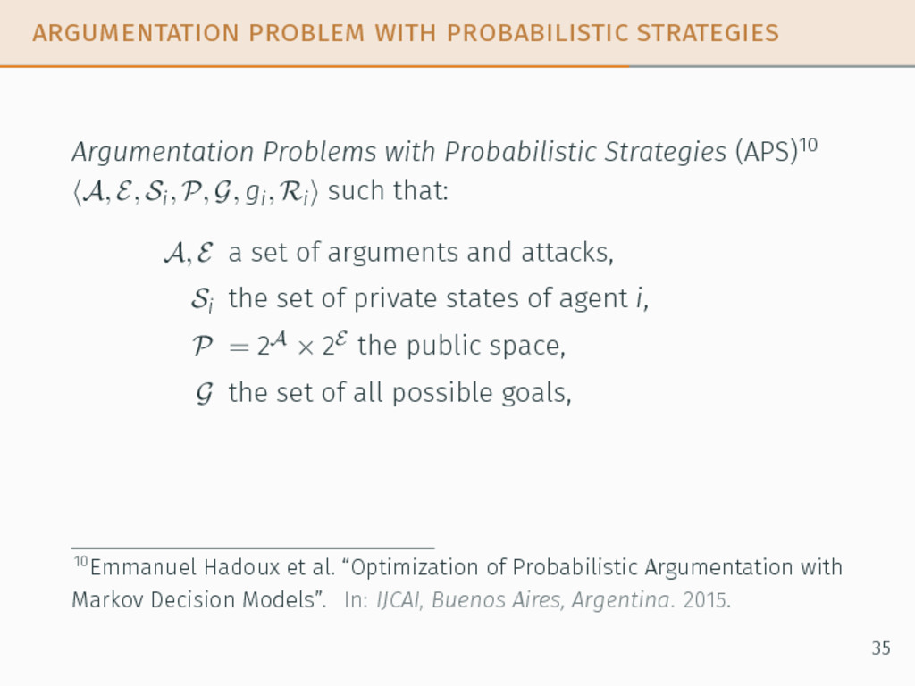
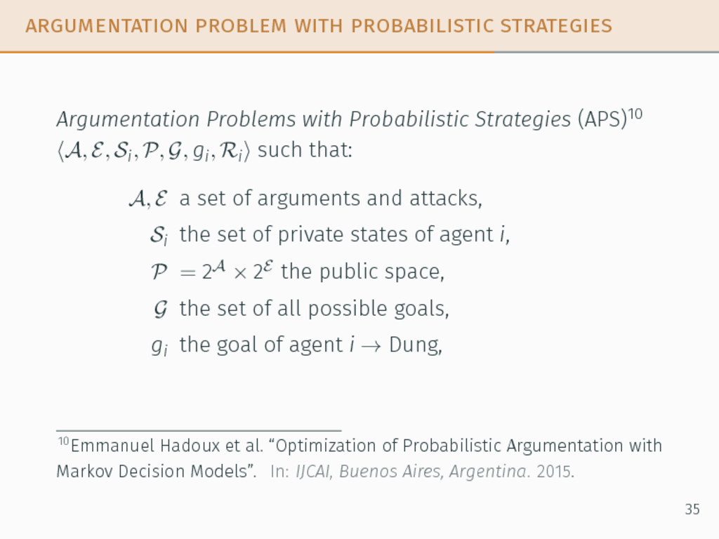
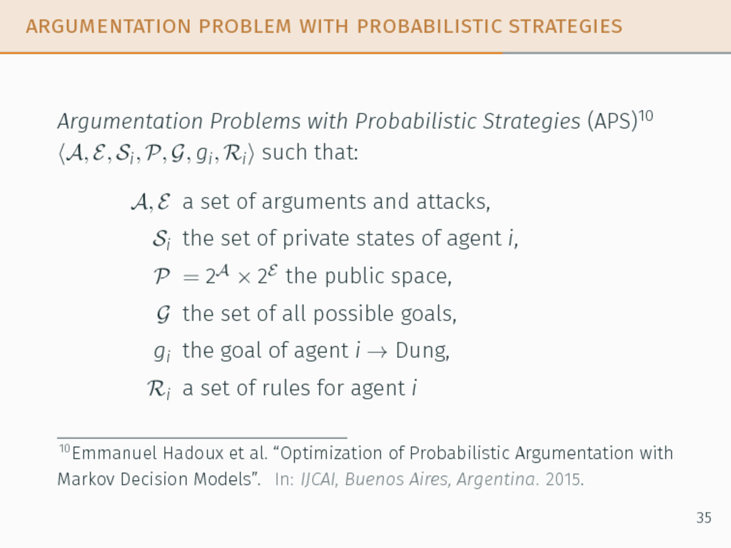
argumentation problem with probabilistic strategies Argumentation Problems with Probabilistic Strategies
(APS)10 ⟨A, E, Si, P, G, gi, Ri⟩ such that: A, E a set of arguments and attacks, 10Emmanuel Hadoux et al. “Optimization of Probabilistic Argumentation with Markov Decision Models”. In: IJCAI, Buenos Aires, Argentina. 2015. 35

(APS)10 ⟨A, E, Si, P, G, gi, Ri⟩ such that: A, E a set of arguments and attacks, Si the set of private states of agent i, 10Emmanuel Hadoux et al. “Optimization of Probabilistic Argumentation with Markov Decision Models”. In: IJCAI, Buenos Aires, Argentina. 2015. 35

(APS)10 ⟨A, E, Si, P, G, gi, Ri⟩ such that: A, E a set of arguments and attacks, Si the set of private states of agent i, P = 2A × 2E the public space, 10Emmanuel Hadoux et al. “Optimization of Probabilistic Argumentation with Markov Decision Models”. In: IJCAI, Buenos Aires, Argentina. 2015. 35

(APS)10 ⟨A, E, Si, P, G, gi, Ri⟩ such that: A, E a set of arguments and attacks, Si the set of private states of agent i, P = 2A × 2E the public space, G the set of all possible goals, 10Emmanuel Hadoux et al. “Optimization of Probabilistic Argumentation with Markov Decision Models”. In: IJCAI, Buenos Aires, Argentina. 2015. 35

(APS)10 ⟨A, E, Si, P, G, gi, Ri⟩ such that: A, E a set of arguments and attacks, Si the set of private states of agent i, P = 2A × 2E the public space, G the set of all possible goals, gi the goal of agent i → Dung, 10Emmanuel Hadoux et al. “Optimization of Probabilistic Argumentation with Markov Decision Models”. In: IJCAI, Buenos Aires, Argentina. 2015. 35

(APS)10 ⟨A, E, Si, P, G, gi, Ri⟩ such that: A, E a set of arguments and attacks, Si the set of private states of agent i, P = 2A × 2E the public space, G the set of all possible goals, gi the goal of agent i → Dung, Ri a set of rules for agent i 10Emmanuel Hadoux et al. “Optimization of Probabilistic Argumentation with Markov Decision Models”. In: IJCAI, Buenos Aires, Argentina. 2015. 35

example: arguments Debate between two agents: Is e-sport a sport?
36

example: arguments Debate between two agents: Is e-sport a sport?
a E-sport is a sport f E-sport is not a physical activity g E-sport is not referenced by IOC a f g b c d e h Figure 3: Attacks graph 36

probabilistic finite state machine: graph APS → Probabilistic Finite State
Machine from an initial state (e.g., {h1(a), h1(b)}, {}, {h2(c), h2(d)}) σ1 start σ2 σ3 σ4 σ5 σ6 σ7 σ8 σ9 σ10 σ11 σ12 1 0.8 0.2 0.5 0.5 1 1 0.8 0.2 0.8 0.2 Figure 4: PFSM of Example e-sport 37

probabilistic finite state machine To optimize the sequence of arguments
for agent 1, we could optimize the PFSM but: 38

for agent 1, we could optimize the PFSM but: 1. depends of the initial state 38

for agent 1, we could optimize the PFSM but: 1. depends of the initial state 2. requires knowledge of the private state of the opponent 38

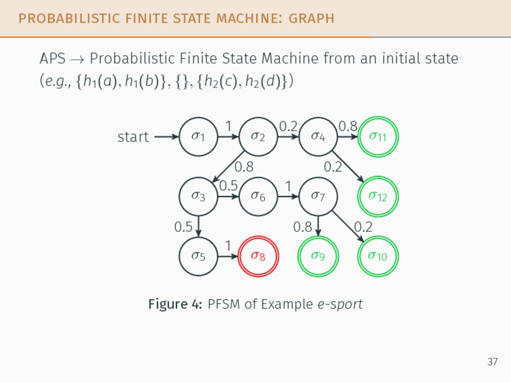
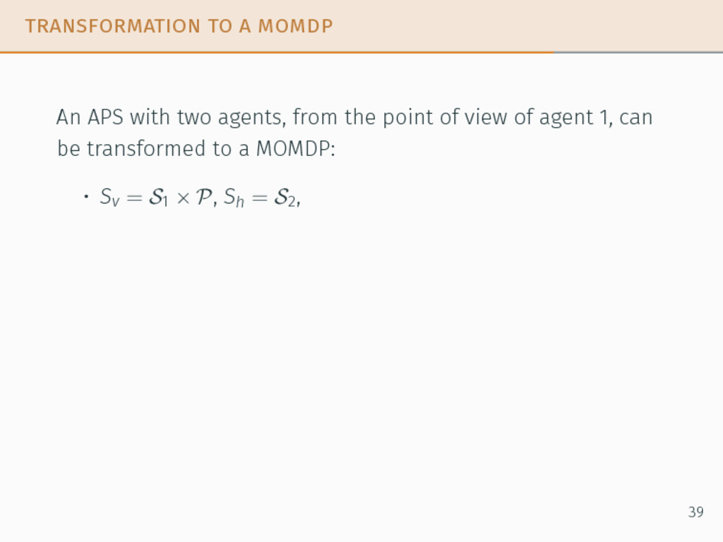
for agent 1, we could optimize the PFSM but: 1. depends of the initial state 2. requires knowledge of the private state of the opponent Using MOMDPs, we can relax assumptions 1 and 2. 38

transformation to a momdp An APS with two agents, from
the point of view of agent 1, can be transformed to a MOMDP: • Sv = S1 × P, Sh = S2 , 39

the point of view of agent 1, can be transformed to a MOMDP: • Sv = S1 × P, Sh = S2 , • Ov = Sv and Oh = ∅, 39

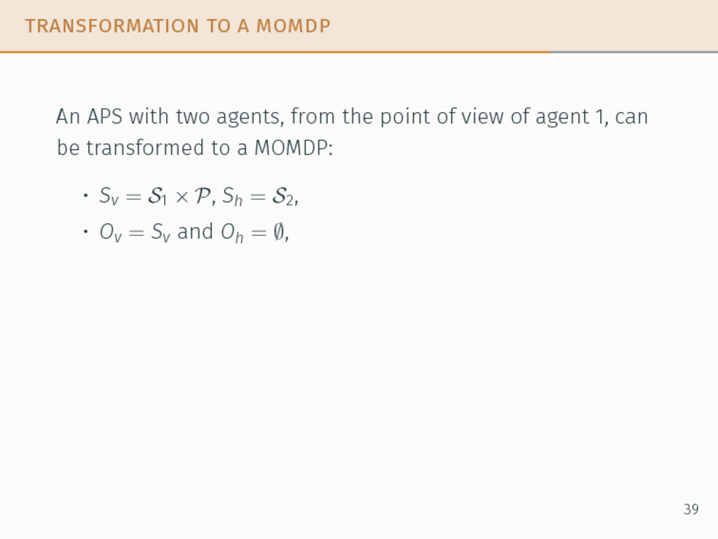
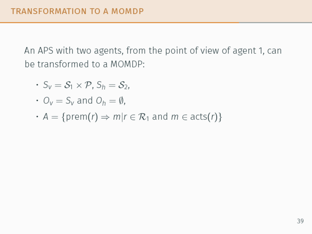
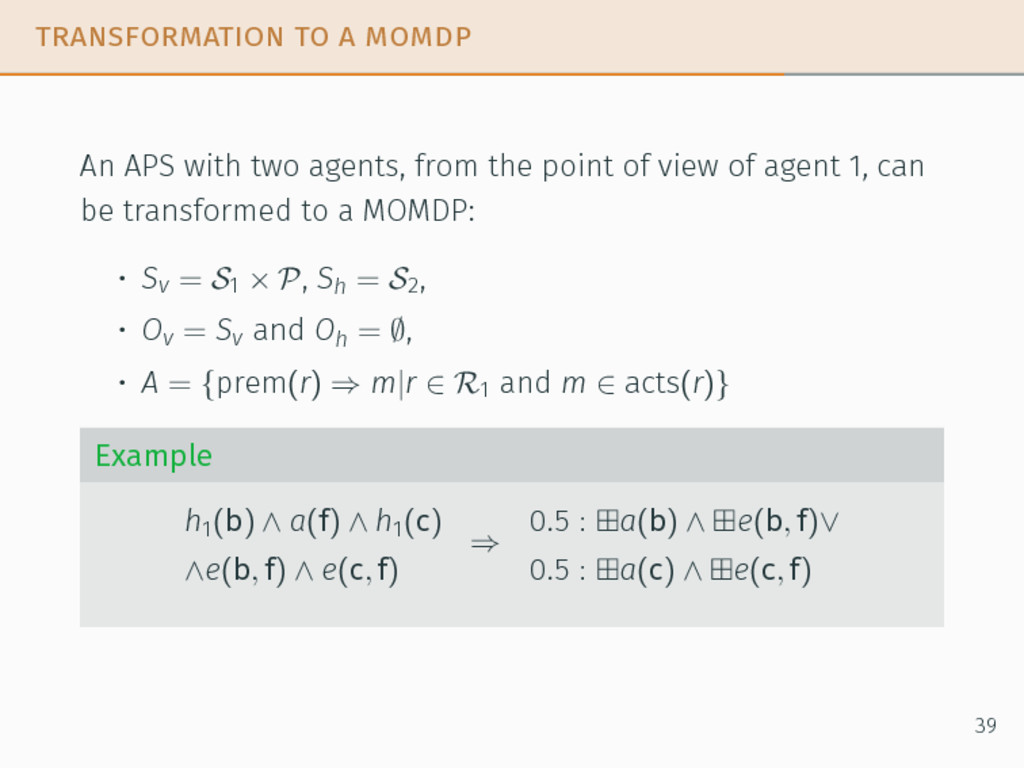
the point of view of agent 1, can be transformed to a MOMDP: • Sv = S1 × P, Sh = S2 , • Ov = Sv and Oh = ∅, • A = {prem(r) ⇒ m|r ∈ R1 and m ∈ acts(r)} 39

the point of view of agent 1, can be transformed to a MOMDP: • Sv = S1 × P, Sh = S2 , • Ov = Sv and Oh = ∅, • A = {prem(r) ⇒ m|r ∈ R1 and m ∈ acts(r)} Example h1(b) ∧ a(f) ∧ h1(c) 0.5 : ⊞a(b) ∧ ⊞e(b, f)∨ ⇒ ∧e(b, f) ∧ e(c, f) 0.5 : ⊞a(c) ∧ ⊞e(c, f) 39

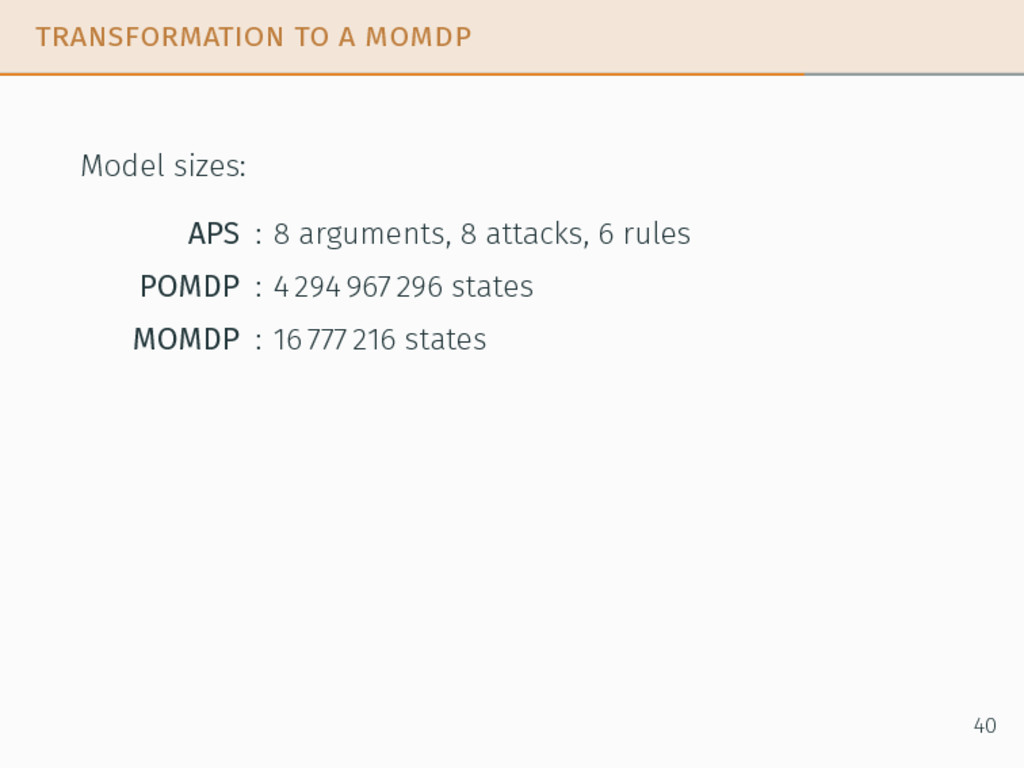
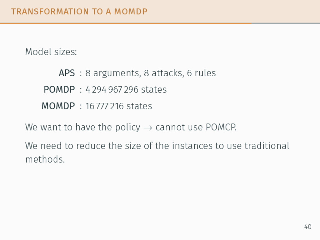
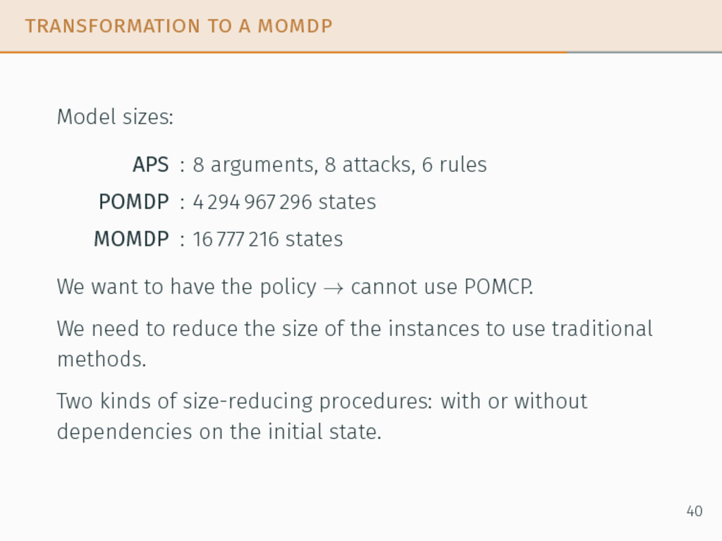
transformation to a momdp Model sizes: APS : 8 arguments,
8 attacks, 6 rules POMDP : 4 294 967 296 states MOMDP : 16 777 216 states 40

8 attacks, 6 rules POMDP : 4 294 967 296 states MOMDP : 16 777 216 states We want to have the policy → cannot use POMCP. We need to reduce the size of the instances to use traditional methods. 40

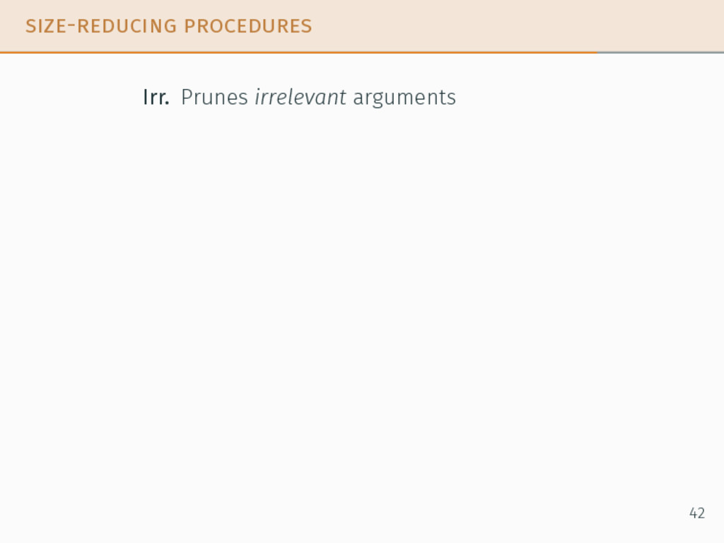
8 attacks, 6 rules POMDP : 4 294 967 296 states MOMDP : 16 777 216 states We want to have the policy → cannot use POMCP. We need to reduce the size of the instances to use traditional methods. Two kinds of size-reducing procedures: with or without dependencies on the initial state. 40

size-reducing procedures Dom. Removes dominated arguments Argument dominance If an
argument is attacked by at least one unattacked argument, it is dominated. a f g b c d e h Figure 5: Attacks graph 41

size-reducing procedures Irr. Prunes irrelevant arguments 42

size-reducing procedures Irr. Prunes irrelevant arguments Irr(s0 ) Removes rules
incompatible with initial state. 42

incompatible with initial state. Enth. Infers attacks 42

incompatible with initial state. Enth. Infers attacks Optimal sequence of procedures 1. Irr(s0 ), Irr. until stable 2. Dom., 1. until stable 3. Enth. 42

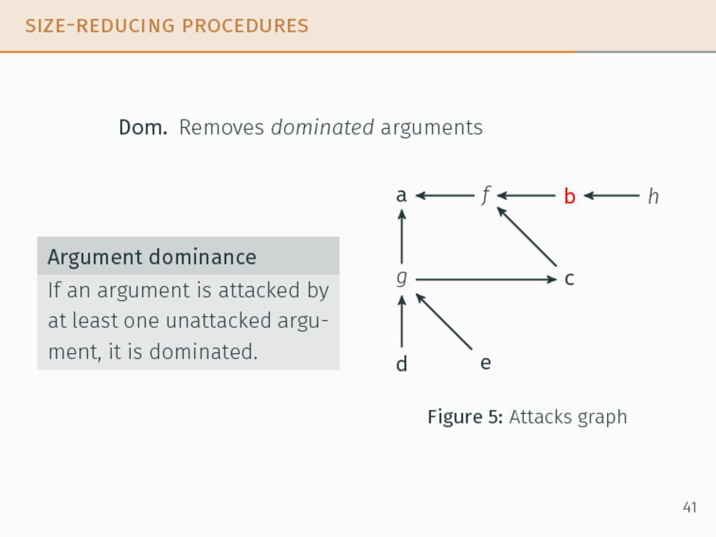
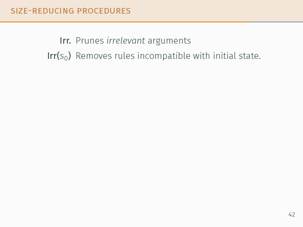
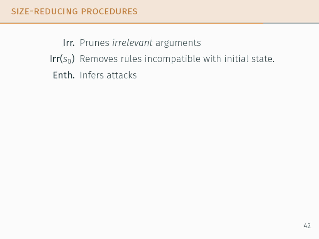
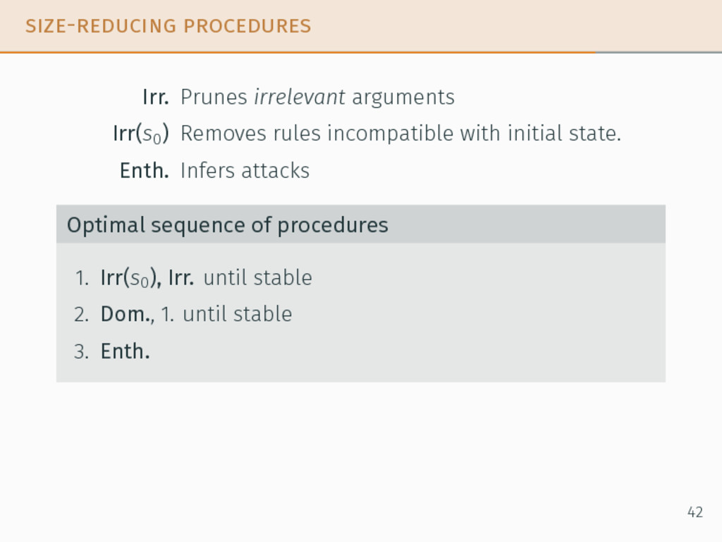
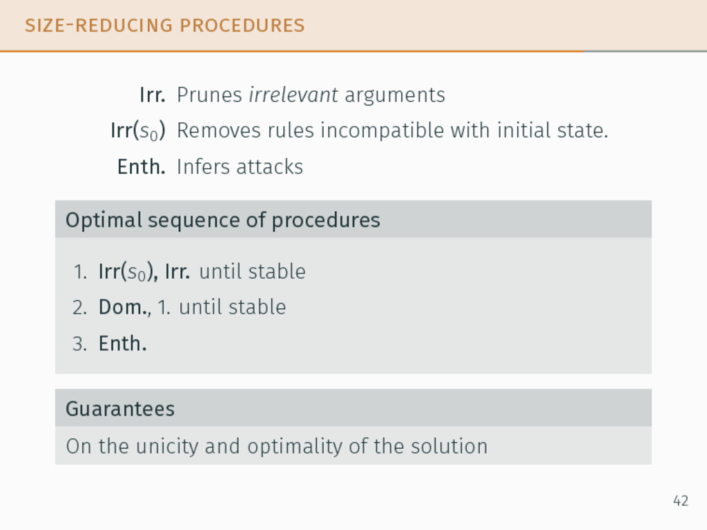
incompatible with initial state. Enth. Infers attacks Optimal sequence of procedures 1. Irr(s0 ), Irr. until stable 2. Dom., 1. until stable 3. Enth. Guarantees On the unicity and optimality of the solution 42

experiments Solution for the e-sport problem computed with MO-SARSOP11. None
Irr. Enth. Dom. Irr(s0 ). All E-sport — — — — — 0.56 6 args 1313 22 43 7 2.4 0.9 7 args — 180 392 16 20 6.7 8 args — — — — 319 45 9 args — — — — — — Table 1: Computation time (in seconds) — means ∞ 11S.C.W. Ong et al. “Planning under uncertainty for robotic tasks with mixed observability”. In: The International Journal of Robotics Research. 2010. 43

mediation problems Let us consider a debate problem with several
agents split in teams. 12Elise Bonzon and Nicolas Maudet. “On the outcomes of multiparty persuasion”. In: AAMAS. 2011, pp. 47–54. 13Michal Chalamish and Sarit Kraus. “AutoMed: an automated mediator for multi-issue bilateral negotiations”. In: JAAMAS 24.3 (2012), pp. 536–564. 44

agents split in teams. We need a mediator to give the speak-turns. 12Elise Bonzon and Nicolas Maudet. “On the outcomes of multiparty persuasion”. In: AAMAS. 2011, pp. 47–54. 13Michal Chalamish and Sarit Kraus. “AutoMed: an automated mediator for multi-issue bilateral negotiations”. In: JAAMAS 24.3 (2012), pp. 536–564. 44

agents split in teams. We need a mediator to give the speak-turns. In most cases, the mediator is not active12 or is looking for a consensus13. 12Elise Bonzon and Nicolas Maudet. “On the outcomes of multiparty persuasion”. In: AAMAS. 2011, pp. 47–54. 13Michal Chalamish and Sarit Kraus. “AutoMed: an automated mediator for multi-issue bilateral negotiations”. In: JAAMAS 24.3 (2012), pp. 536–564. 44

agents split in teams. We need a mediator to give the speak-turns. In most cases, the mediator is not active12 or is looking for a consensus13. We envision a more active mediator with her own agenda → generalization 12Elise Bonzon and Nicolas Maudet. “On the outcomes of multiparty persuasion”. In: AAMAS. 2011, pp. 47–54. 13Michal Chalamish and Sarit Kraus. “AutoMed: an automated mediator for multi-issue bilateral negotiations”. In: JAAMAS 24.3 (2012), pp. 536–564. 44

mediation problems in non-stationary environments We also consider each agent
can be either of the two following modes: 14Still under review. 45

can be either of the two following modes: constructive argumenting towards the goal, 14Still under review. 45

can be either of the two following modes: constructive argumenting towards the goal, destructive argumenting against the opponent’s goal. 14Still under review. 45

can be either of the two following modes: constructive argumenting towards the goal, destructive argumenting against the opponent’s goal. But other modes can be deﬁned. 14Still under review. 45

can be either of the two following modes: constructive argumenting towards the goal, destructive argumenting against the opponent’s goal. But other modes can be deﬁned. We proposed Dynamic Mediation Problems (DMP)14 for those problems from the viewpoint of the mediator. 14Still under review. 45

conversion to a hs3mdp The argumentative modes can be converted
into HS3MDP modes, allowing us to convert DMPs to HS3MDPs. 46

into HS3MDP modes, allowing us to convert DMPs to HS3MDPs. We can solve the problem using our adaptations of POMCP. 46

into HS3MDP modes, allowing us to convert DMPs to HS3MDPs. We can solve the problem using our adaptations of POMCP. Purpose Organize the sequence of speak-turns for the mediator. 46

conclusion To apply decision-making to argumentation, we proposed: • A
formalization of debates with probabilistic strategies (APS), 47

formalization of debates with probabilistic strategies (APS), • How to transform APS to MOMDP and solve them, 47

formalization of debates with probabilistic strategies (APS), • How to transform APS to MOMDP and solve them, • Size-reducing procedures, 47

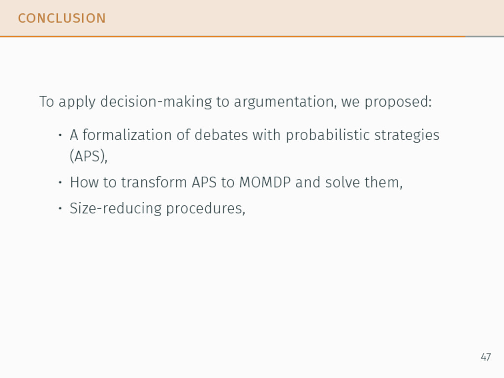
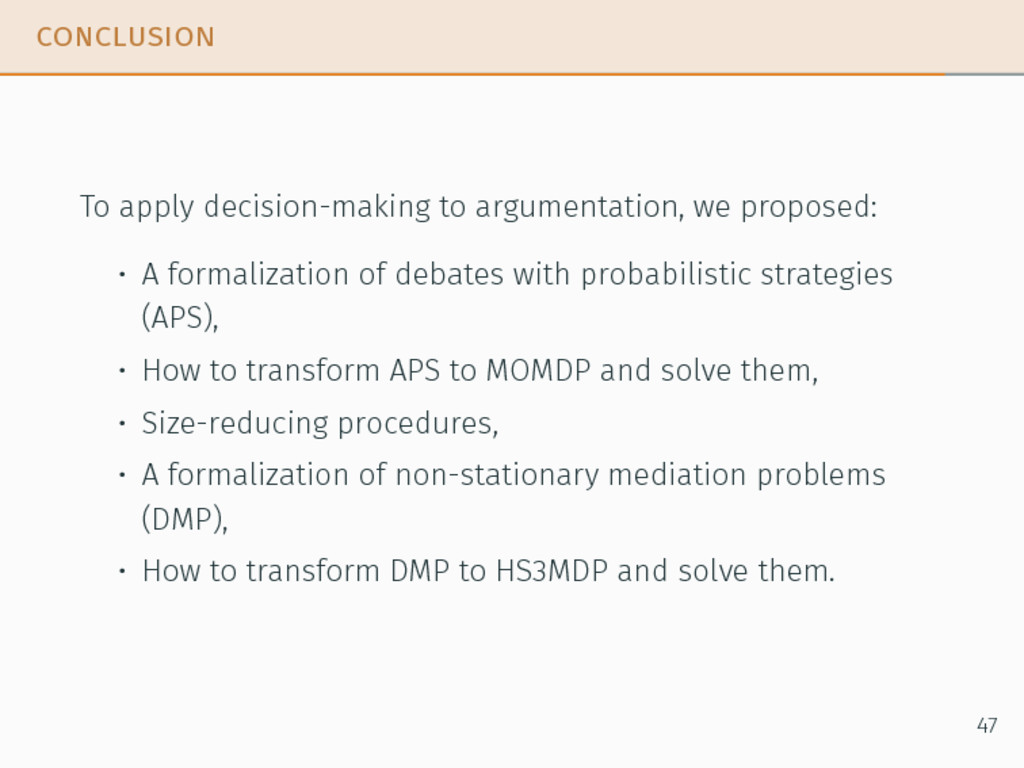
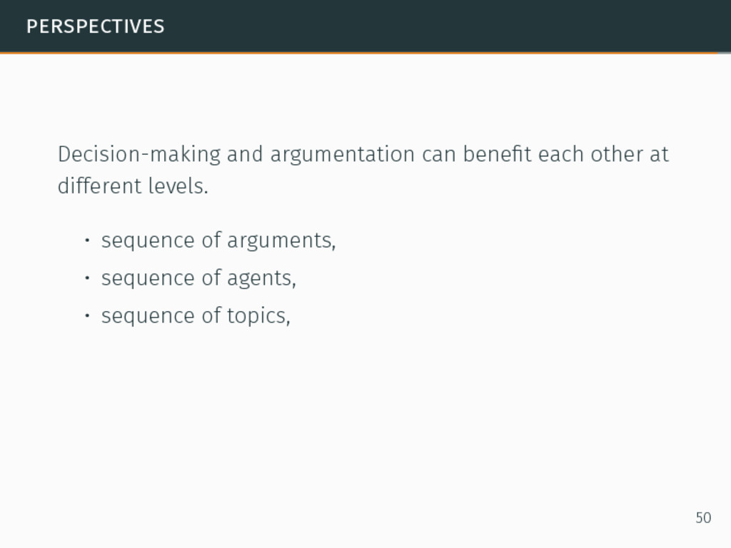
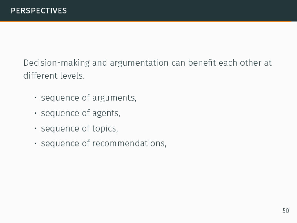
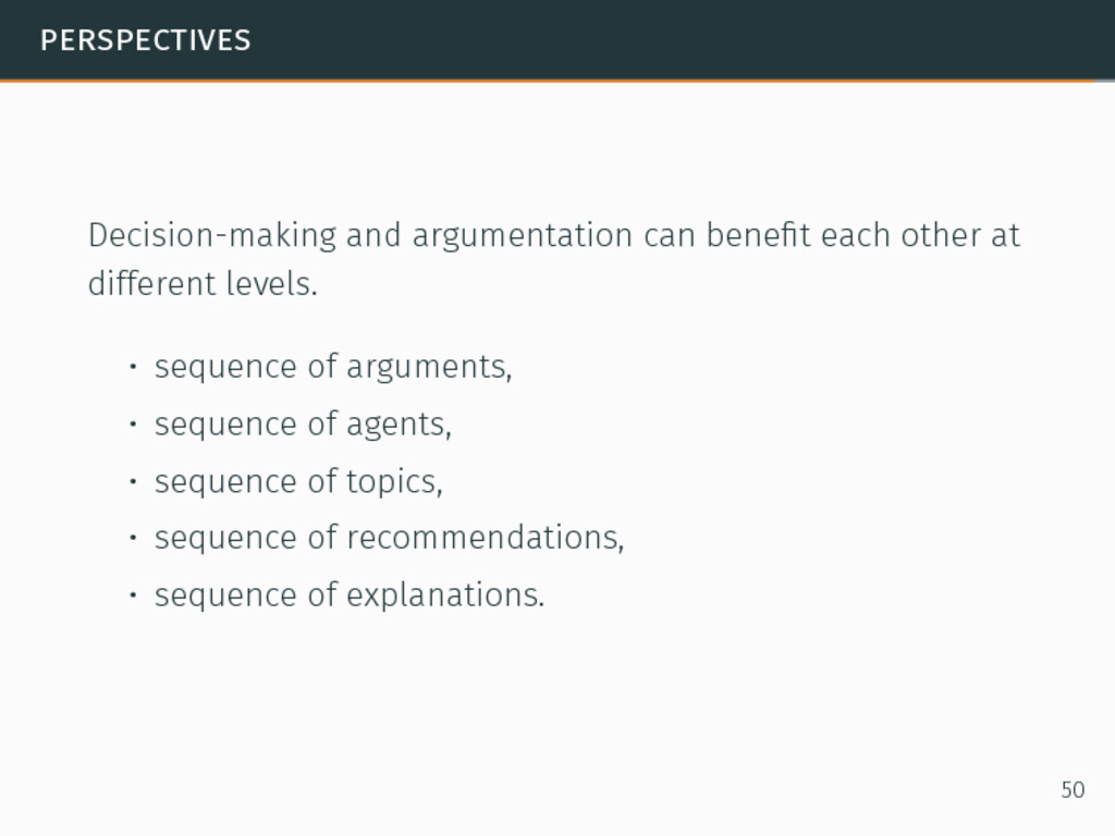
formalization of debates with probabilistic strategies (APS), • How to transform APS to MOMDP and solve them, • Size-reducing procedures, • A formalization of non-stationary mediation problems (DMP), 47

formalization of debates with probabilistic strategies (APS), • How to transform APS to MOMDP and solve them, • Size-reducing procedures, • A formalization of non-stationary mediation problems (DMP), • How to transform DMP to HS3MDP and solve them. 47

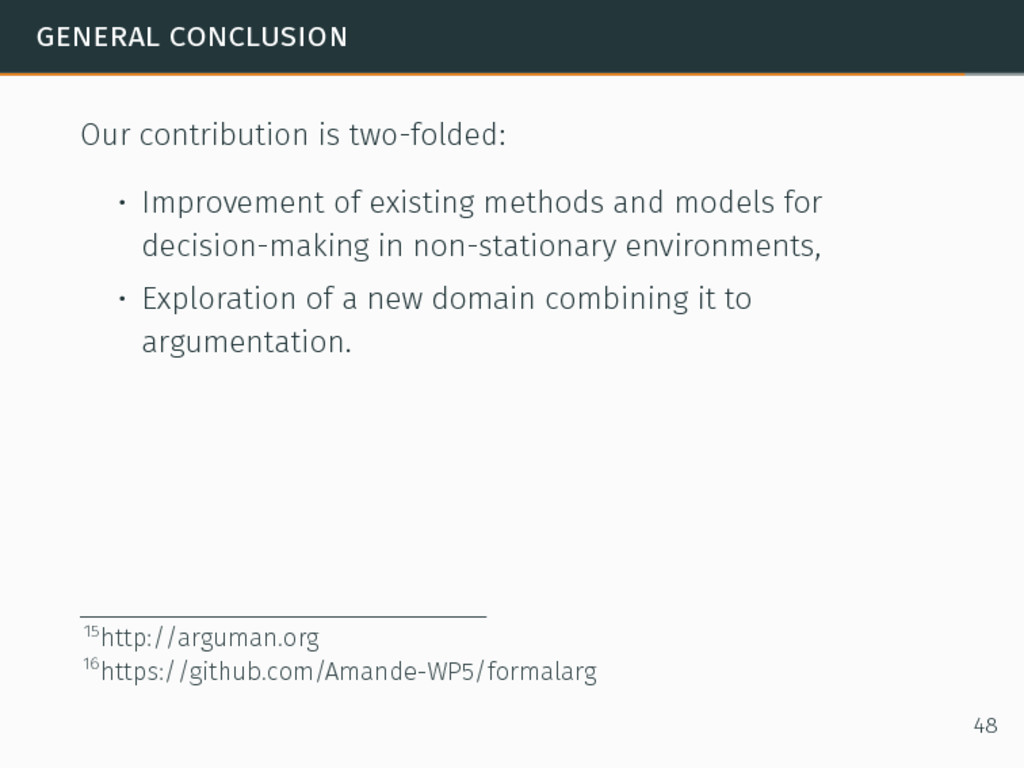
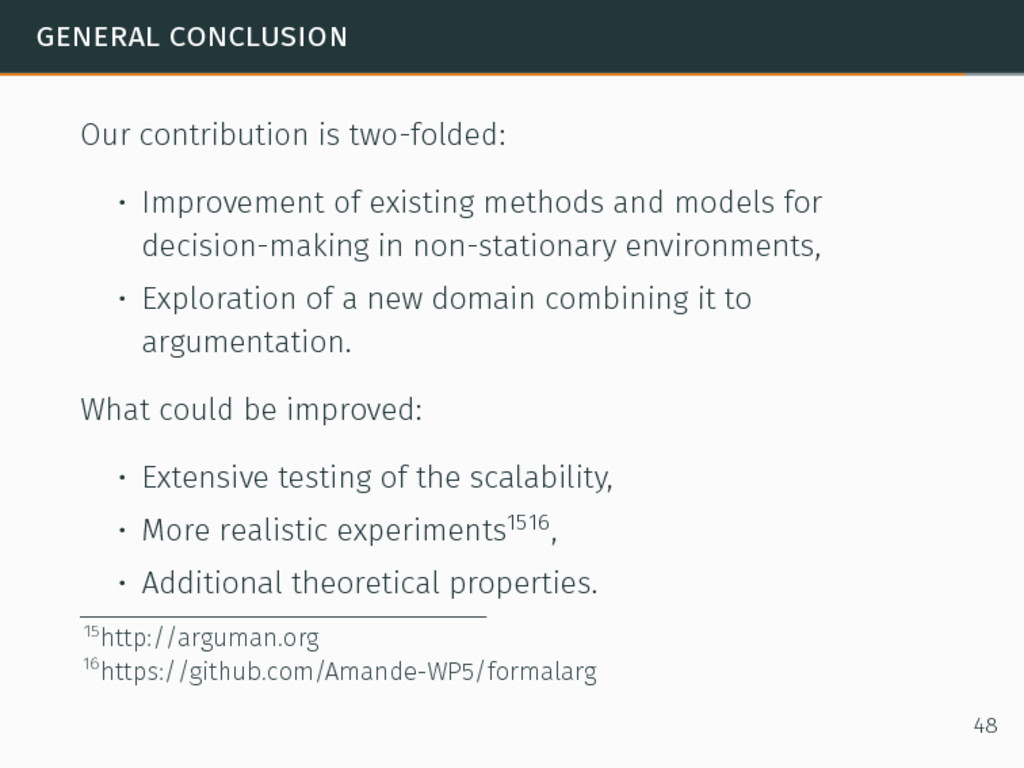
general conclusion Our contribution is two-folded: • Improvement of existing
methods and models for decision-making in non-stationary environments, • Exploration of a new domain combining it to argumentation. 15http://arguman.org 16https://github.com/Amande-WP5/formalarg 48

general conclusion Our contribution is two-folded: • Improvement of existing
methods and models for decision-making in non-stationary environments, • Exploration of a new domain combining it to argumentation. What could be improved: • Extensive testing of the scalability, • More realistic experiments1516, • Additional theoretical properties. 15http://arguman.org 16https://github.com/Amande-WP5/formalarg 48

perspectives Some straightforward follow-ups of this work: • learn the
mode transition/duration functions in HS3MDPs, • develop our adaptations of POMCP for MOMDPs, 49

perspectives Some straightforward follow-ups of this work: • learn the
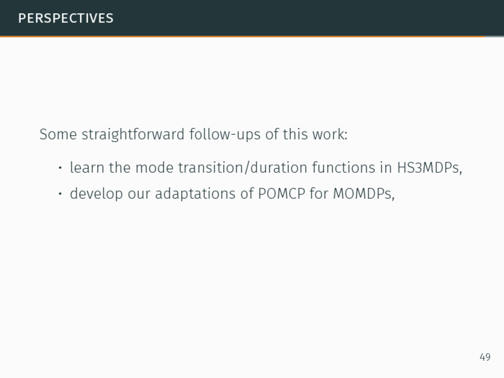
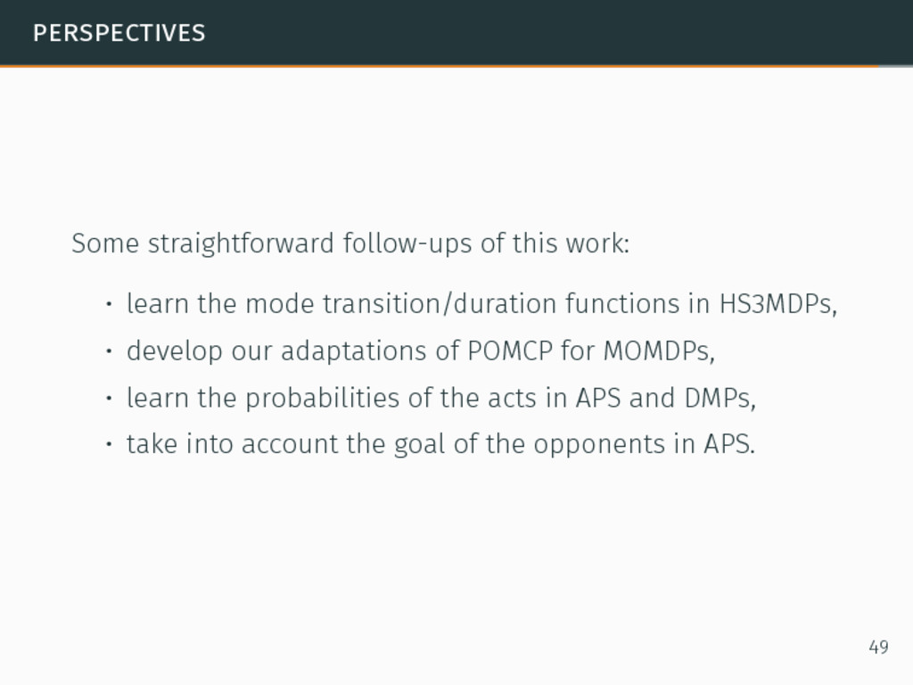
mode transition/duration functions in HS3MDPs, • develop our adaptations of POMCP for MOMDPs, • learn the probabilities of the acts in APS and DMPs, • take into account the goal of the opponents in APS. 49

perspectives Decision-making and argumentation can beneﬁt each other at different
levels. • sequence of arguments, 50

levels. • sequence of arguments, • sequence of agents, 50

levels. • sequence of arguments, • sequence of agents, • sequence of topics, 50

levels. • sequence of arguments, • sequence of agents, • sequence of topics, • sequence of recommendations, 50

levels. • sequence of arguments, • sequence of agents, • sequence of topics, • sequence of recommendations, • sequence of explanations. 50

Thank you very much for you attention 51

Markovian sequential decision-making in non-stationary environments: application to argumentation problems

Markovian sequential decision-making in non-stationary environments: application to argumentation problems

More Decks by Emmanuel Hadoux

Other Decks in Research

Featured

Transcript