Network Approaches Reveal the Complexity of Chinese Dialect History

Talk held at The 8th Conference of the European Association of Chinese Linguistics, September 26-28, EHESS, Paris.

Transcript

1. . . . . . . . Network Approaches Reveal the Complexity of Chinese Dialect History Johann-Mattis List∗ ∗Research Center Deutscher Sprachatlas Philipps-University Marburg 2013/09/26 1 / 30
2. 语言 language 1 язык språk 1 Languages 2 / 30
3. Languages and Dialects Norwegian, Danish, and Swedish are different languages. . . Běijīng-Chinese, Shànghǎi-Chinese, and Hakka-Chinese are dialects of the same Chinese language. 3 / 30
4. Languages and Dialects Beijing Chinese 1 iou²¹ i⁵⁵ xuei³⁵ pei²¹fəŋ⁵⁵ kən⁵⁵ tʰai⁵¹iaŋ¹¹ t͡ʂəŋ⁵⁵ ʦai⁵³ naɚ⁵¹ t͡ʂəŋ⁵⁵luən⁵¹ Hakka Chinese 1 iu³³ it⁵⁵ pai³³a¹¹ pet³³fuŋ³³ tʰuŋ¹¹ ɲit¹¹tʰeu¹¹ hɔk³³ e⁵³ au⁵⁵ Shanghai Chinese 1 ɦi²² tʰɑ̃⁵⁵ ʦɿ²¹ poʔ³foŋ⁴⁴ taʔ⁵ tʰa³³ɦiã⁴⁴ ʦəŋ³³ hɔ⁴⁴ ləʔ¹lə²³ʦa⁵³ Beijing Chinese 2 ʂei³⁵ də⁵⁵ pən³⁵ liŋ²¹ ta⁵¹ Hakka Chinese 2 man³³ ɲin¹¹ kʷɔ⁵⁵ vɔi⁵³ Shanghai Chinese 2 sa³³ ɲiŋ⁵⁵ ɦəʔ²¹ pəŋ³³ zɿ⁴⁴ du¹³ Norwegian 1 nuːɾɑʋinˑn̩ ɔ suːln̩ kɾɑŋlət ɔm Swedish 1 nuːɖanvɪndən ɔ suːlən tv̥ɪstadə ən gɔŋ ɔm Danish 1 noʌ̯ʌnvenˀn̩ ʌ soːl̩ˀn kʰʌm eŋg̊ɑŋ i sd̥ʁiðˀ ʌmˀ Norwegian 2 ʋem ɑ dem sɱ̩ ʋɑː ɖɳ̩ stæɾ̥kəstə Swedish 2 vɛm ɑv dɔm sɔm vɑ staɹkast Danish 2 vɛmˀ a b̥m̩ d̥ vɑ d̥n̩ sd̥æʌ̯g̊əsd̥ə 4 / 30
5. Languages and Dialects From the perspective of the lexicon and the sound system, the Chinese dialects are at least equally if not more different than the Scandinavian languages. 4 / 30
6. Language as a Diasystem Languages are complex aggregates of different linguistic systems that‘coexist and influence each other’(Coseriu 1973: 40, my translation). . . 5 / 30
7. Language as a Diasystem Languages are complex aggregates of different linguistic systems that‘coexist and influence each other’(Coseriu 1973: 40, my translation). . . A linguistic diasystem requires a “roof language” (Goossens 1973:11), i.e. a linguistic variety that serves as a standard for interdialectal communication. 5 / 30
8. Language as a Diasystem Standard Language Diatopic Varieties Diastratic Varieties Diaphasic Varieties 6 / 30
9. Modeling Language History 7 / 30
10. Dendrophilia August Schleicher (1821-1868) 8 / 30
11. Dendrophilia August Schleicher (1821-1868) These assumptions that logically fol- low from the results of our re- search can be best illustrated with help of a branching tree. (Schleicher 1853: 787, my translation) 8 / 30
12. Dendrophilia Schleicher (1853) 9 / 30
13. Dendrophobia Johannes Schmidt (1843-1901) 10 / 30
14. Dendrophobia Johannes Schmidt (1843-1901) No matter how we look at it, as long as we stick to the assumption that today’s languages originated from their common proto-language via multiple furcation, we will never be able to explain all facts in a scientifi- cally adequate way. (Schmidt 1872: 17, my translation) 10 / 30
15. Dendrophobia Johannes Schmidt (1843-1901) I want to replace [the tree] by the im- age of a wave that spreads out from the center in concentric circles be- coming weaker and weaker the far- ther they get away from the center. (Schmidt 1872: 27, my translation) 11 / 30
16. Dendrophobia Schmidt (1875) 12 / 30
17. Dendrophobia Meillet (1908) Hirt (1905) Bloomfield (1933) Bonfante (1931) 13 / 30
18. Phylogenetic Networks Trees are bad, because 14 / 30
19. Phylogenetic Networks Trees are bad, because they are so difficult to reconstruct............ 14 / 30
20. Phylogenetic Networks Trees are bad, because they are so difficult to reconstruct............ languages do not separate in split processes 14 / 30
21. Phylogenetic Networks Trees are bad, because they are so difficult to reconstruct............ languages do not separate in split processes they are boring, since they only capture the vertical aspects of language history 14 / 30
22. Phylogenetic Networks Trees are bad, because they are so difficult to reconstruct............ languages do not separate in split processes they are boring, since they only capture the vertical aspects of language history Waves are bad, because nobody knows how to reconstruct them 14 / 30
23. Phylogenetic Networks Trees are bad, because they are so difficult to reconstruct............ languages do not separate in split processes they are boring, since they only capture the vertical aspects of language history Waves are bad, because nobody knows how to reconstruct them languages still separate, even if not in split processes 14 / 30
24. Phylogenetic Networks Trees are bad, because they are so difficult to reconstruct............ languages do not separate in split processes they are boring, since they only capture the vertical aspects of language history Waves are bad, because nobody knows how to reconstruct them languages still separate, even if not in split processes they are boring, since they only capture the horizontal aspects of language history 14 / 30
25. Phylogenetic Networks Hugo Schuchardt (1842-1927) 15 / 30
26. Phylogenetic Networks Hugo Schuchardt (1842-1927) We connect the branches and twigs of the tree with countless horizon- tal lines and it ceases to be a tree (Schuchardt 1870 [1900]: 11) 15 / 30
27. Phylogenetic Networks 16 / 30
28. 魚 1 魚 1 魚 1 ? 首首 首 首 Modelling Chinese Dialect History 17 / 30
29. Data 18 / 30
30. Data Data was taken from the 现代汉语方言音库 Xiàndài Hànyǔ Fāngyán Yīnkù (Hóu 2004). 18 / 30
31. Data Data was taken from the 现代汉语方言音库 Xiàndài Hànyǔ Fāngyán Yīnkù (Hóu 2004). 180 items (“concepts”), translated into 40 dialect varieties of Chinese. 18 / 30
32. Data Data was taken from the 现代汉语方言音库 Xiàndài Hànyǔ Fāngyán Yīnkù (Hóu 2004). 180 items (“concepts”), translated into 40 dialect varieties of Chinese. Original source provides the data in RTF format (phonetic transcription, proposed underlying characters) along with audio files. 18 / 30
33. Data Data was taken from the 现代汉语方言音库 Xiàndài Hànyǔ Fāngyán Yīnkù (Hóu 2004). 180 items (“concepts”), translated into 40 dialect varieties of Chinese. Original source provides the data in RTF format (phonetic transcription, proposed underlying characters) along with audio files. RTF data was converted to text-format in order to allow automatic comparison. 18 / 30
34. Data Data was taken from the 现代汉语方言音库 Xiàndài Hànyǔ Fāngyán Yīnkù (Hóu 2004). 180 items (“concepts”), translated into 40 dialect varieties of Chinese. Original source provides the data in RTF format (phonetic transcription, proposed underlying characters) along with audio files. RTF data was converted to text-format in order to allow automatic comparison. All entries were compared with the original transcriptions and the audio-files in order to decrease the number of errors that might have resulted from the conversion or the transcriptions. 18 / 30
35. Data ITEM 太阳 tàiyáng “sun” . Dialect Pronunciation Character Cognacy 上海 Shanghai tʰa³⁴⁻³³ɦiã¹³⁻⁴⁴ 太阳 1 上海 Shànghǎi ȵjɪʔ¹⁻¹¹dɤ¹³⁻²³ 日头 2 温州 Wénzhōu tʰa⁴²⁻²²ji 太阳 1 温州 Wénzhōu ȵi²¹³⁻²²dɤu 日头 2 广州 Guǎngzhōu jit²tʰɐu²¹⁻³⁵ 热头 3 广州 Guǎngzhōu tʰai³³jœŋ²¹ 太阳 1 海口 Hǎikǒu zit³hau³¹ 日头 2 北京 Běijīng tʰai⁵¹iɑŋ¹ 太阳 1 19 / 30
36. dummy . . Guānhuà . Xiàng . Mǐn . Yuè . Wú . Jìn . Kèjiā . Gàn . Pínghuà . Huī . 1 . 2 . 3 . 4 . 5 . 6 . 7 . 8 . 9 . 10 . 11 . 12 . 13 . 14 . 15 . 16 . 17 . 18 . 19 . 20 . 21 . 22 . 23 . 24 . 25 . 26 . 27 . 28 . 29 . 30 . 31 . 32 . 33 . 34 . 35 . 36 . 37 . 38 . 39 . 40 . 1 . Běijīng 北京 . 2 . Chángshā 长沙 . 3 . Chéngdū 成都 . 4 . Fùzhōu 福州 . 5 . Guǎngzhōu 广州 . 6 . Guìyáng 贵阳 . 7 . Harbin 哈尔滨 . 8 . Hǎikǒu 海口 . 9 . Hángzhōu 杭州 . 10 . Héfèi 合肥 . 11 . Hohhot 呼和浩特 . 12 . Jiàn'ōu 建瓯 . 13 . Jìnán 济南 . 14 . Kùnmíng 昆明 . 15 . Lánzhōu 兰州 . 16 . Měixiàn 梅县 . 17 . Nánchàng 南昌 . 18 . Nánjīng 南京 . 19 . Nánníng 南宁 . 20 . Píngyáo 平遥 . 21 . Qīngdǎo 青岛 . 22 . Shànghǎi 上海 . 23 . Shāntóu 汕头 . 24 . Shèxiàn 歙县 . 25 . Sùzhōu 苏州 . 26 . Táiběi 台北 . 27 . Tàiyuán 太原 . 28 . Táoyuán 桃园 . 29 . Tiānjìn 天津 . 30 . Tūnxī 屯溪 . 31 . Wénzhōu 温州 . 32 . Wǔhàn 武汉 . 33 . Ürümqi 乌鲁木齐 . 34 . Xiàmén 厦门 . 35 . Hongkong 香港 . 36 . Xiāngtàn 湘潭 . 37 . Xīníng 西宁 . 38 . Xī'ān 西安 . 39 . Yīnchuàn 银川 . 40 . Zhèngzhōu 郑州 . . . . 20 / 30
37. Analysis 21 / 30
38. Analysis The data was analysed with help of an improved version of the minimal lateral network approach (Dagan & Martin 2007, Dagan et al. 2008). 21 / 30
39. Analysis The data was analysed with help of an improved version of the minimal lateral network approach (Dagan & Martin 2007, Dagan et al. 2008). This version is freely available as part of a larger Python library for quantitative tasks in historical linguistics (LingPy, List & Moran 2013). 21 / 30
40. Analysis The data was analysed with help of an improved version of the minimal lateral network approach (Dagan & Martin 2007, Dagan et al. 2008). This version is freely available as part of a larger Python library for quantitative tasks in historical linguistics (LingPy, List & Moran 2013). ▶ Starting from a reference tree that should display the “true” history of the languages as closely as possible, and a set of homologous characters (etymologically related words, cognates), the MLN approach infers horizontal relations between the contemporary and ancestral languages in the reference tree. 21 / 30
41. Analysis The data was analysed with help of an improved version of the minimal lateral network approach (Dagan & Martin 2007, Dagan et al. 2008). This version is freely available as part of a larger Python library for quantitative tasks in historical linguistics (LingPy, List & Moran 2013). ▶ Starting from a reference tree that should display the “true” history of the languages as closely as possible, and a set of homologous characters (etymologically related words, cognates), the MLN approach infers horizontal relations between the contemporary and ancestral languages in the reference tree. ▶ For each character (cognate set), a specific scenario which is closest to the patterns observed in the rest of the data is reconstructed. 21 / 30
42. Analysis The data was analysed with help of an improved version of the minimal lateral network approach (Dagan & Martin 2007, Dagan et al. 2008). This version is freely available as part of a larger Python library for quantitative tasks in historical linguistics (LingPy, List & Moran 2013). ▶ Starting from a reference tree that should display the “true” history of the languages as closely as possible, and a set of homologous characters (etymologically related words, cognates), the MLN approach infers horizontal relations between the contemporary and ancestral languages in the reference tree. ▶ For each character (cognate set), a specific scenario which is closest to the patterns observed in the rest of the data is reconstructed. ▶ The main criterion for the selection of scenarios is homogeneity of the distribution of words across a fixed set of meanings in the sample. 21 / 30
43. Analysis The data was analysed with help of an improved version of the minimal lateral network approach (Dagan & Martin 2007, Dagan et al. 2008). This version is freely available as part of a larger Python library for quantitative tasks in historical linguistics (LingPy, List & Moran 2013). ▶ Starting from a reference tree that should display the “true” history of the languages as closely as possible, and a set of homologous characters (etymologically related words, cognates), the MLN approach infers horizontal relations between the contemporary and ancestral languages in the reference tree. ▶ For each character (cognate set), a specific scenario which is closest to the patterns observed in the rest of the data is reconstructed. ▶ The main criterion for the selection of scenarios is homogeneity of the distribution of words across a fixed set of meanings in the sample. ▶ As a result, the method detects patterns that are suggestive of borrowing (patchy cognate sets). These can be directly reported to the researcher for further analysis or displayed in form of a rooted network. 21 / 30
44. Analysis The data was analysed with help of an improved version of the minimal lateral network approach (Dagan & Martin 2007, Dagan et al. 2008). This version is freely available as part of a larger Python library for quantitative tasks in historical linguistics (LingPy, List & Moran 2013). ▶ Starting from a reference tree that should display the “true” history of the languages as closely as possible, and a set of homologous characters (etymologically related words, cognates), the MLN approach infers horizontal relations between the contemporary and ancestral languages in the reference tree. ▶ For each character (cognate set), a specific scenario which is closest to the patterns observed in the rest of the data is reconstructed. ▶ The main criterion for the selection of scenarios is homogeneity of the distribution of words across a fixed set of meanings in the sample. ▶ As a result, the method detects patterns that are suggestive of borrowing (patchy cognate sets). These can be directly reported to the researcher for further analysis or displayed in form of a rooted network. The reference tree used for the analysis is based on Laurent Sagart’s (pers. comm.) proposal for an innovation-based subgrouping of the Chinese dialects in which 瓦乡 Wǎxiāng and 蔡家 Càijiā (both not in our data) are taken as as primary branches. 21 / 30
45. Analysis -- Spanish -- French -- Italian Danish -- English -- German -- 22 / 30
46. Analysis -- Spanish -- French -- Italian Danish -- English -- German -- 22 / 30
47. Analysis -- Spanish -- French -- Italian Danish -- English -- German -- 22 / 30
48. Analysis -- Spanish -- French -- Italian Danish -- English -- German -- 22 / 30
49. Analysis Sounds nice, but how good does the method work? 23 / 30
50. Analysis Sounds nice, but how good does the method work? A test on 40 Indo-European languages showed that out of 105 cognate sets containing known borrowings, 76 were correctly identified as such. 23 / 30
51. Analysis Sounds nice, but how good does the method work? A test on 40 Indo-European languages showed that out of 105 cognate sets containing known borrowings, 76 were correctly identified as such. Of 19 borrowings in English, 17 were correctly identified by the method. 23 / 30
52. Analysis Ok, nice, but isn’t there anything else you forgot to say? 24 / 30
53. Analysis Ok, nice, but isn’t there anything else you forgot to say? As our test on the Indo-European data revealed, the method does not only detect borrowings. It detects all kinds of errors in the data. Among these are: 24 / 30
54. Analysis Ok, nice, but isn’t there anything else you forgot to say? As our test on the Indo-European data revealed, the method does not only detect borrowings. It detects all kinds of errors in the data. Among these are: ▶ Cases of parallel semantic shift that look like borrowings for the method. 24 / 30
55. Analysis Ok, nice, but isn’t there anything else you forgot to say? As our test on the Indo-European data revealed, the method does not only detect borrowings. It detects all kinds of errors in the data. Among these are: ▶ Cases of parallel semantic shift that look like borrowings for the method. ▶ Erroneous cognate judgments that also look like borrowings. 24 / 30
56. Analysis Ok, nice, but isn’t there anything else you forgot to say? As our test on the Indo-European data revealed, the method does not only detect borrowings. It detects all kinds of errors in the data. Among these are: ▶ Cases of parallel semantic shift that look like borrowings for the method. ▶ Erroneous cognate judgments that also look like borrowings. ▶ Methodological errors (deep etymologies although the stochastic models require shallow ones, fuzzy concepts as basis, erroneous translations). 24 / 30
57. Analysis Ok, nice, but isn’t there anything else you forgot to say? As our test on the Indo-European data revealed, the method does not only detect borrowings. It detects all kinds of errors in the data. Among these are: ▶ Cases of parallel semantic shift that look like borrowings for the method. ▶ Erroneous cognate judgments that also look like borrowings. ▶ Methodological errors (deep etymologies although the stochastic models require shallow ones, fuzzy concepts as basis, erroneous translations). It is certainly a benefit, that we can use the method to clean our data, but we should be careful with the results and only use it as an initial heuristic. 24 / 30
58. Results: General 56% of the characters cannot be explained with help of the reference tree. 25 / 30
59. Results: General 56% of the characters cannot be explained with help of the reference tree. This proportion is almost two times higher than was inferred for Indo-European (31%, 40 languages, 207 semantic items). 25 / 30
60. Results: General 56% of the characters cannot be explained with help of the reference tree. This proportion is almost two times higher than was inferred for Indo-European (31%, 40 languages, 207 semantic items). Results might result from the fact that the concepts do not exclusively represent “basic concepts” (Swadesh 1952) and are thus more prone to borrowing. However, we don’t find a significant difference (p = 0.16, using Wilcoxon’s rank sum test) between between basic and non-basic concepts and the rest of the concepts. 25 / 30
61. Sardinian Rumanian Italian French Provencal Catalan Portuguese Spanish Albanian Greek Armenian Irish Breton Welsh Norwegian Danish Swedish Faroese Icelandic Dutch Frisian English German Latvian Lithuanian Bulgarian Slovenian Serbocroatian Russian Byelorussian Ukrainian Czech Slovak Polish Hindi Urdu Ossetic Pashto Kurdish Persian Sardinian Rumanian Italian French Provencal Catalan Portuguese Spanish Albanian Greek Armenian Irish Breton Welsh Norwegian Danish Swedish Faroese Icelandic Dutch Frisian English German Latvian Lithuanian Bulgarian Slovenian Serbocroatian Russian Byelorussian Ukrainian Czech Slovak Polish Hindi Urdu Ossetic Pashto Kurdish Persian 0.1 0.2 0.3 0.4 0.5 0.6 0.7 0.8 0.9 1.0 Shared Cognates Shared cognate percentages (Indo-European) 26 / 30
62. . . . Tàiyuán . Píngyáo . Hohhot . Xī'ān . Xīníng . Zhèngzhōu . Lánzhōu . Yīnchuàn . Ürümqi . Tiānjìn . Jìnán . Qīngdǎo . Běijīng . Harbin . Guìyáng . Kùnmíng . Chéngdū . Wǔhàn . Nánjīng . Héfèi . Xiāngtàn . Chángshā . Nánchàng . Shèxiàn . Tūnxī . Shànghǎi . Sùzhōu . Hángzhōu . Wénzhōu . Hongkong . Guǎngzhōu . Nánníng . Měixiàn . Táoyuán . Xiàmén . Táiběi . Shāntóu . Hǎikǒu . Fùzhōu . Jiàn'ǒu . Tàiyuán . Píngyáo . Hohhot . Xī'ān . Xīníng . Zhèngzhōu . Lánzhōu . Yīnchuàn . Ürümqi . Tiānjìn . Jìnán . Qīngdǎo . Běijīng . Harbin . Guìyáng . Kùnmíng . Chéngdū . Wǔhàn . Nánjīng . Héfèi . Xiāngtàn . Chángshā . Nánchàng . Shèxiàn . Tūnxī . Shànghǎi . Sùzhōu . Hángzhōu . Wénzhōu . Hongkong . Guǎngzhōu . Nánníng . Měixiàn . Táoyuán . Xiàmén . Táiběi . Shāntóu . Hǎikǒu . Fùzhōu . Jiàn'ǒu . 0.32 . 0.40 . 0.48 . 0.56 . 0.64 . 0.72 . 0.80 . 0.88 . 0.96 . Shared Cognates Shared cognate percentages (Chinese) 26 / 30
63. Albanian_St Irish_A Welsh_N Breton_List Sardinian French Provencal Italian Catalan Spanish Portuguese Rumanian English Icelandic_S Faroese Norwegian Danish Swedish German Dutch_List Frisian Slovenian Bulgarian Serbocroati Russian Czech Slovak Polish Ukrainian Byelorussia Latvian Lithuanian Hindi Urdu Pashto Persian Kurdish Digor_Osset Armenian_Mo Greek_Mod 0.1 Neighbor-Net Analysis (Indo-European) 26 / 30
64. Beijing Tianjin Haerbin Zhengzhou Yinchuan Wulumuqi Huhehaote Taiyuan Pingyao Xi’an Lanzhou Xining Kunming Guiyang Chengdu Changsha Xiangtan Nanchang Hangzhou Shanghai Suzhou Shexian Tunxi Jian’ou Fuzhou Haikou Shantou Xiamen Taibei Taoyuan Meixian Wenzhou Xianggang Guangzhou Nanning Wuhan Nanjing Hefei Qingdao Jinan 0.1 Neighbor-Net Analysis (Chinese) 26 / 30
65. Results: Minimal Lateral Network ---Lánzhōu Fùzhōu -- Xiāngtàn -- M ěixiàn -- H ongkong -- ---Wǔhàn ---Běijīng ---Kùnmíng Hángzhōu -- Xiàmén -- ---Chéngdū Sùzhōu -- Shànghǎi -- Táiběi -- ---Zhèngzhōu Shèxiàn -- ---Nánjīng ---Guìyáng W énzhōu -- N ánníng -- Tūnxī -- ---Tiānjìn Shāntóu -- ---Xīníng ---Q īngdǎo ---Ürüm qi ---Píngyáo Nánchàng -- ---Tàiyuán Chángshā -- Hǎikǒu -- ---Héfèi Jiàn'ǒu -- ---Yīnchuàn ---Hohhot Táoyuán -- ---Xī'ān G uǎngzhōu -- ---Harbin ---Jìnán Reference tree of the Chinese dialects 27 / 30
66. Results: Minimal Lateral Network ---Lánzhōu Fùzhōu -- Xiāngtàn -- M ěixiàn -- H ongkong -- ---Wǔhàn ---Běijīng ---Kùnmíng Hángzhōu -- Xiàmén -- ---Chéngdū Sùzhōu -- Shànghǎi -- Táiběi -- ---Zhèngzhōu Shèxiàn -- ---Nánjīng ---Guìyáng W énzhōu -- N ánníng -- Tūnxī -- ---Tiānjìn Shāntóu -- ---Xīníng ---Q īngdǎo ---Ürüm qi ---Píngyáo Nánchàng -- ---Tàiyuán Chángshā -- Hǎikǒu -- ---Héfèi Jiàn'ǒu -- ---Yīnchuàn ---Hohhot Táoyuán -- ---Xī'ān G uǎngzhōu -- ---Harbin ---Jìnán MLN analysis, no borrowing allowed 27 / 30
67. Results: Minimal Lateral Network ---Lánzhōu Fùzhōu -- Xiāngtàn -- M ěixiàn -- H ongkong -- ---Wǔhàn ---Běijīng ---Kùnmíng Hángzhōu -- Xiàmén -- ---Chéngdū Sùzhōu -- Shànghǎi -- Táiběi -- ---Zhèngzhōu Shèxiàn -- ---Nánjīng ---Guìyáng W énzhōu -- N ánníng -- Tūnxī -- ---Tiānjìn Shāntóu -- ---Xīníng ---Q īngdǎo ---Ürüm qi ---Píngyáo Nánchàng -- ---Tàiyuán Chángshā -- Hǎikǒu -- ---Héfèi Jiàn'ǒu -- ---Yīnchuàn ---Hohhot Táoyuán -- ---Xī'ān G uǎngzhōu -- ---Harbin ---Jìnán MLN analysis, best fit of borrowing and inheritance 27 / 30
68. Results: Minimal Lateral Network . . Guānhuà . Xiàng . Mǐn . Yuè . Wú . Jìn . Kèjiā . Gàn . Huī . 1 . 2 . 3 . 4 . 5 . 6 . 7 . 8 . 9 . 10 . 11 . 12 . 13 . 14 . 15 . 16 . 17 . 18 . 19 . 20 . 21 . 22 . 23 . 24 . 25 . 26 . 27 . 28 . 29 . 30 . 31 . 32 . 33 . 34 . 35 . 36 . 37 . 38 . 39 . 40 . 1 . Běijīng 北京 . 2 . Chángshā 长沙 . 3 . Chéngdū 成都 . 4 . Fùzhōu 福州 . 5 . Guǎngzhōu 广州 . 6 . Guìyáng 贵阳 . 7 . Harbin 哈尔滨 . 8 . Hǎikǒu 海口 . 9 . Hángzhōu 杭州 . 10 . Héfèi 合肥 . 11 . Hohhot 呼和浩特 . 12 . Jiàn'ōu 建瓯 . 13 . Jìnán 济南 . 14 . Kùnmíng 昆明 . 15 . Lánzhōu 兰州 . 16 . Měixiàn 梅县 . 17 . Nánchàng 南昌 . 18 . Nánjīng 南京 . 19 . Nánníng 南宁 . 20 . Píngyáo 平遥 . 21 . Qīngdǎo 青岛 . 22 . Shànghǎi 上海 . 23 . Shāntóu 汕头 . 24 . Shèxiàn 歙县 . 25 . Sùzhōu 苏州 . 26 . Táiběi 台北 . 27 . Tàiyuán 太原 . 28 . Táoyuán 桃园 . 29 . Tiānjìn 天津 . 30 . Tūnxī 屯溪 . 31 . Wénzhōu 温州 . 32 . Wǔhàn 武汉 . 33 . Ürümqi 乌鲁木齐 . 34 . Xiàmén 厦门 . 35 . Hongkong 香港 . 36 . Xiāngtàn 湘潭 . 37 . Xīníng 西宁 . 38 . Xī'ān 西安 . 39 . Yīnchuàn 银川 . 40 . Zhèngzhōu 郑州 . . . . 27 / 30
69. Results: Specific Scenarios . . -----Jìnán . -----Harbin . -----Héfèi . Chángshā ---- . Sùzhōu ---- . -----Yīnchuàn . -----Běijīng . Hángzhōu ---- . -----Chéngdū . -----Hohhot . -----Lánzhōu . Xiāngtàn ---- . -----Ürüm qi . M ěixiàn ---- . -----Xī'ān . G uǎngzhōu ---- . -----Nánjīng . Táoyuán ---- . -----Zhèngzhōu . -----Kùnmíng . Táiběi ---- . Shànghǎi ---- . Xiàmén ---- . Jiàn'ǒu ---- . Shèxiàn ---- . -----Q īngdǎo . -----Xīníng . Fùzhōu ---- . -----Tàiyuán . -----Píngyáo . Nánchàng ---- . H ongkong ---- . N ánníng ---- . W énzhōu ---- . -----Guìyáng . Shāntóu ---- . -----Tiānjìn . Tūnxī ---- . Hǎikǒu ---- . -----Wǔhàn . 太阳 . 日头 . 热头 . 阳婆 . 日 . Loss Event . Gain Event Item „sun” 28 / 30
70. Results: Specific Scenarios Item „sun” . . Shànghǎi ---- . Hongkong ---- . Táiběi ---- . Nánjīng ---- . Táoyuán ---- . Běijīng ---- . Měixiàn ---- . Xiàmén ---- . Fùzhōu ---- . Guǎngzhōu ---- . 太阳 . 日头 . Loss Event . Gain Event 28 / 30
71. Results: Specific Scenarios Item „sun” . . Shànghǎi ---- . Hongkong ---- . Táiběi ---- . Nánjīng ---- . Táoyuán ---- . Běijīng ---- . Měixiàn ---- . Xiàmén ---- . Fùzhōu ---- . Guǎngzhōu ---- . 太阳 . 日头 . Loss Event . Gain Event 28 / 30
72. Results: Specific Scenarios Item „sun” . . Shànghǎi ---- . Hongkong ---- . Táiběi ---- . Nánjīng ---- . Táoyuán ---- . Běijīng ---- . Měixiàn ---- . Xiàmén ---- . Fùzhōu ---- . Guǎngzhōu ---- . 太阳 . 日头 . Loss Event . Gain Event 28 / 30
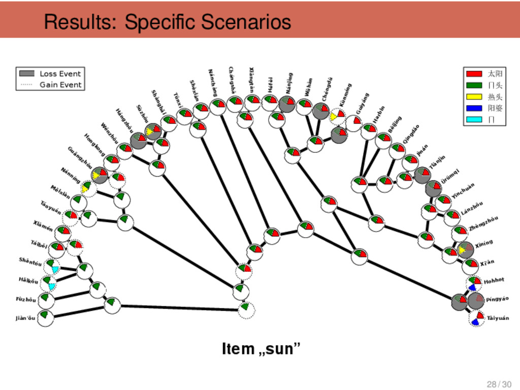
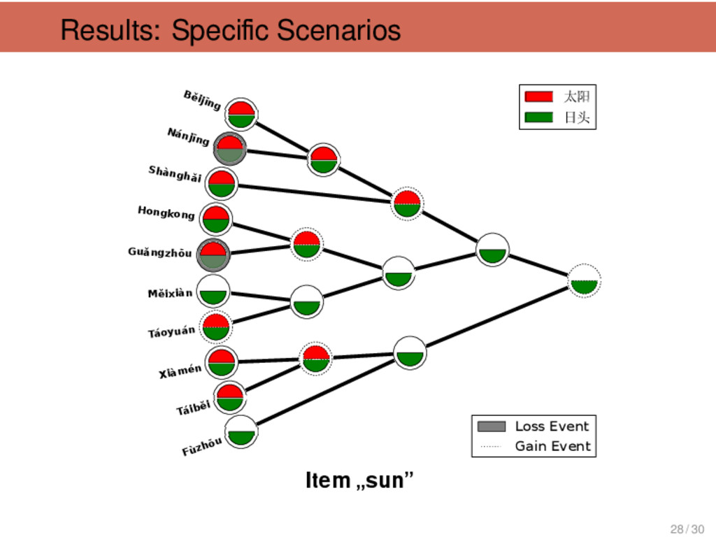
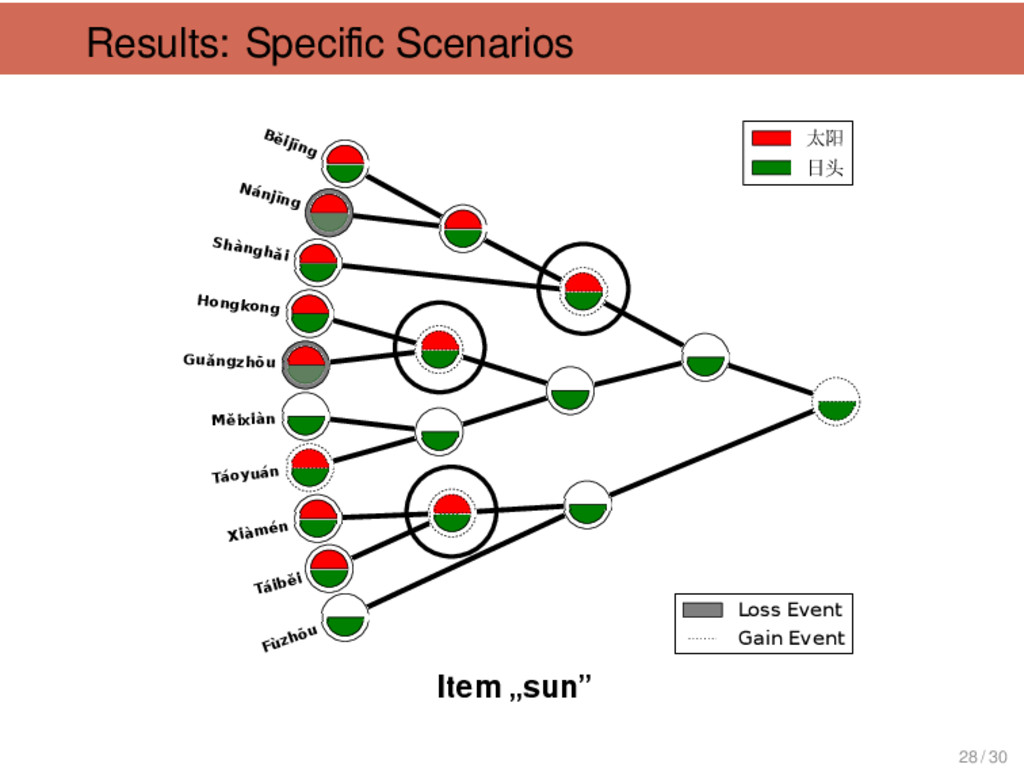
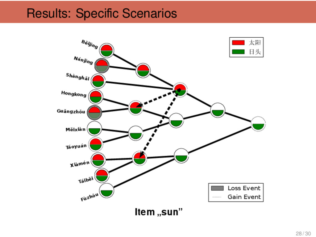
73. Resultats: Specific Links Node Weight Cognate Sets Hǎikǒu non-Mǐn 7 刚 刚 “just (just came)”, 淡 “light”, 南 瓜 “pumpkin”, 菠 菜 “spinach”, 勺 “spoon”, 瘦 “thin”, 从 “from” Tàiběi, Xiàmén non-Mǐn 6 只 “only”, 中 秋 节 “Mid- Autumn Festival”, 房间 “flat”, 只 classifier (cow), 冷 “cold”, 只 classifier (pig) Tàiběi, Xiàmén Táoyuán 6 豆 油 “soya sauce”, 包 仔 “baozi”, 太阳 “sun”, 桌仔“ta- ble”, 对 “from”, 看医生“go to the doctor” Shànghǎi Shèxiàn 6 彩 虹 “rainbow”, 女 人 “wife”, 爷 “father”, 落苏 “aubergine”, 山芋 “sweet potato”, 洋山芋 “spinach” Hángzhōu Mandarin, Huī, Xiàng, Gàn, Jìn 6 里头 “inside”, 哪个 “who”, 哪 里 “where”, 那个 “that”, 刚好 “just right”, 包心菜 “cabbage” 29 / 30
74. Conclusion and Outlook Phylogenetic networks look nice. Phylogenetic networks can provide an alternative to both trees and waves. The application of phylogenetic network analyses in historical linguistics is still in its infancy. We have to test the methods further in order to get a better impression on its strong and weak points. 30 / 30
75. Conclusion and Outlook 谢谢大家！ 30 / 30
76. Conclusion and Outlook Thank you! 30 / 30