Upgrade to Pro — share decks privately, control downloads, hide ads and more …

Getting started with Sparse Modeling with spm-image

Hacarus Inc.
September 21, 2019

Getting started with Sparse Modeling with spm-image

Presentation slides at PyCon Taiwan 2019 (https://tw.pycon.org/2019)

Hacarus Inc.

September 21, 2019
Tweet

More Decks by Hacarus Inc.

Other Decks in Technology

Transcript

  1. PyCon Taiwan 2019 Getting started with Sparse Modeling with spm-image

    Takashi Someda CTO, Hacarus Inc. September 21st, 2019
  2. About Me Takashi Someda, @tksmd Director/CTO at HACARUS Inc. Master’s

    degree of Information Science at Kyoto University Sun Microsystems K.K. → Founded own startup at Kyoto → Established Kyoto Branch of Nulab Inc. → Current
  3. Today’s Takeaways • Basic concept of Sparse Modeling • Image

    and time series data analysis • Guide to Python examples using spm-image
  4. Blackbox Problem Blackbox AI Target Result Blackbox AI cannot answer

    questions like • Why do I get the result ? • When does it succeed/fail ? • How can I correct the result ? difficult to use AI even if it shows fascinating performance
  5. Approach to explainable AI • Post-hoc explain a given AI

    model • Individual prediction explanations • Global prediction explanations • Build an interpretable model • Logistic regression, Decision trees and so on For more details, refer to Explainable AI in Industry (KDD 2019 Tutorial)
  6. Lacking or missing data • Tiny dataset • Data augmentation

    • Transfer Learning in Deep Learning • Missing values • Imputation of mean values, using regression, etc • Use missing value friendly model
  7. History of Sparse Modeling Year Paper Author 1996 Regression Shrinkage

    and Selection via Lasso R. Tibshirani 1996 Sparse Coding B. Olshausen 2006 Compressed Sensing D.L. Donoho 2018 Multi-Layer Convolutional Sparse Modeling M. Elad
  8. • Problem Settings • Output y can be expressed as

    linear combination of x with observation noise ε where x is m dimensional and sample size of y is n = $ $ + ⋯ + ( ( + Basic approach to the problem • Least squares method • Minimize least square errors of y and multipliers of x and estimated w min 1 2 − 0
  9. What if data is not sufficient ? → Assume that

    not all input features won’t be used to express y • Additional constraint will be introduced as regularization term • Objective function can be changed to the following form min 1 2 − 0 + 3 ⇒ Regularization parameter λ controls effectiveness of regularization Introduce Regularization
  10. • L0 norm optimization • Use minimum number of x

    to satisfy equation • Find w to minimize number of non-zero elements • Combinational optimization • NP-hard and not feasible L L0 and L1 norm optimization • L1 norm optimization • Find w to minimize sum of its absolute values • Global solution can (still) be reached • Solved within practical time Relax constraint Least Absolute Shrinkage and Selection Operator
  11. spm-image • Python library for Sparse Modeling (OSS) • https://github.com/hacarus/spm-image/

    • scikit-learn compliant interface • supported algorithms and planned works • generalized Lasso (4 variants) • k-svd and more… • total variation, more lasso (planned) • more examples (planned)
  12. # scikit-learn from sklearn.linear_model import Lasso model = Lasso(alpha=0.1) model.fit(X_train,

    Y_train) model.score(X_test, y_test) # spm-image from spmimage.linear_model import LassoADMM as Lasso model = Lasso (alpha=0.1) model.fit(X_train, Y_train) model.score(X_test, y_test) Code: scikit-learn and spm-image
  13. X is 1,000 dimensional input features Only 20 features out

    of 1,000 are relevant to output y Only 100 samples are available Example: Numerical experiment
  14. Compressed Sensing • Problem Settings • y: observed data A:

    observation, then estimate x with sparse constraint Lasso • Objective functions http://mriquestions.com/what-is-k-space.html (image source of k-space) k-space MRI Fourier Transform
  15. Total Variation min 7 − 0 + ∇ $ Total

    Variation TV makes an image smooth while keeping edge
  16. 1. Extract patches from images 2. Learn dictionary to express

    every patches 3. Every patches should be represented as sparse combination of dictionary basis Y: Image A: Dictionary : < < X: coefficient Dictionary Learning
  17. Dictionary (8x8, 64 basis) Sparse Coding (green is 0) Example:

    Image Reconstruction Sparse Encode Reconstruction
  18. # extract patches patches = extract_simple_patches_2d(img, patch_size) # normalize patches

    patches = patches.reshape(patches.shape[0], -1).astype(np.float64) intercept = np.mean(patches, axis=0) patches -= intercept patches /= np.std(patches, axis=0) # dictionary learning model = KSVD(n_components=n_basis, alpha=1, n_iter=n_iter, n_jobs=1) model.fit(patches) # reconstruction reconstructed_patches = np.dot(code, model.components_) reconstructed_patches = reconstructed_patches.reshape(len(patches), *patch_size) reconstructed = reconstruct_from_simple_patches_2d(reconstructed_patches, img.shape) Code: Image Reconstruction
  19. X = extract_and_flatten(img, patch_size) # normalize values except missing values

    X = np.where(X == 0, -9999, X) for idx in range(X.shape[0]): target_idx = np.where(X[idx, :] != -9999) target = X[idx, target_idx] t_mean = np.mean(target) t_std = np.std(target) X[idx, target_idx] = (target - t_mean)/t_std # fit with missing values model = KSVD(n_components=n_components, transform_n_nonzero_coefs=k0, max_iter=10, missing_value=-9999, method='approximate’) model.fit(X) Code: Inpainting
  20. Anomaly Detection Dictionary feature extraction Sparse code Dataset of only

    “Good” images Reconstruction Error PSNR/SSIM… Test image Classifier Result
  21. Example: Defect detection Proposed methods(paper below) and Dictionary Learning based

    approach https://arxiv.org/abs/1807.02894 Paper (SVM) Paper (CNN) Dictionary Learning Dataset 800 images 800 images 60 images Training time 30 mins 5 hours 19 secs Inference time 8 mins 20 secs 10 secs Accuracy 85% 86% 90% Monocrystalline modules
  22. Generalized Lasso Lasso Generalized Lasso • Problem Settings (again) •

    y: observed data A: observation, then estimate x with sparse constraint • Objective functions
  23. Constraint Design Constraint for 1st order differential 2 neighboring values

    tends to be same Fused Lasso Trend Filtering Constraint for 2nd order differential 3 neighboring values tends to be on straight line
  24. Code: Fused Lasso class FusedLassoADMM(GeneralizedLasso): def __init__(self, alpha=1.0, sparse_coef=1.0, trend_coef=1.0,

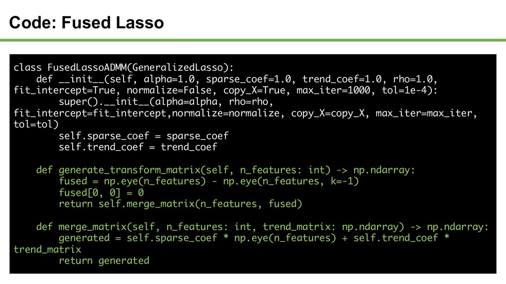
    rho=1.0, fit_intercept=True, normalize=False, copy_X=True, max_iter=1000, tol=1e-4): super().__init__(alpha=alpha, rho=rho, fit_intercept=fit_intercept,normalize=normalize, copy_X=copy_X, max_iter=max_iter, tol=tol) self.sparse_coef = sparse_coef self.trend_coef = trend_coef def generate_transform_matrix(self, n_features: int) -> np.ndarray: fused = np.eye(n_features) - np.eye(n_features, k=-1) fused[0, 0] = 0 return self.merge_matrix(n_features, fused) def merge_matrix(self, n_features: int, trend_matrix: np.ndarray) -> np.ndarray: generated = self.sparse_coef * np.eye(n_features) + self.trend_coef * trend_matrix return generated
  25. Code: Trend Filtering class TrendFilteringADMM(FusedLassoADMM): def generate_transform_matrix(self, n_features: int) ->

    np.ndarray: trend = 2 * np.eye(n_features) - np.eye(n_features, k=-1) - np.eye(n_features, k=1) trend[0, 0] = 1 trend[-1:, -1] = 1 return self.merge_matrix(n_features, trend)
  26. Example: Numerical experiment • True trend is sin wave (blue)

    • Gaussian noise is added to observed data (red) • Estimated trend is fitted by Trend Filtering using Generalized Lasso (green)
  27. Sparse Modeling in a nutshell • Small dataset, explainable, lightweight

    • Applicable to image and time series data • Has been developed over 20 years and still evolving
  28. Sparse Modeling vs Other SOTA ML methods Sparse Modeling Other

    SOTA ML methods Makes rule from data and prior information, i.e. sparsity Makes rule (basically) only from data Can start with small dataset and both training and inference is fast Requires big dataset with a lot of time for training Focus on specific use cases Can support very wide range of problem