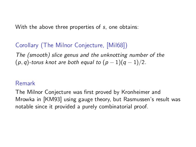
the colored Jones polynomial and Rasmussen invariant of links”. In: Canad. J. Math. 60.6 (2008), pp. 1240–1266. [Kho06] M. Khovanov. “Link homology and Frobenius extensions”. In: Fund. Math. 190 (2006), pp. 179–190. [KM93] P. B. Kronheimer and T. S. Mrowka. “Gauge theory for embedded surfaces. I”. In: Topology 32.4 (1993), pp. 773–826. [Lee05] E. S. Lee. “An endomorphism of the Khovanov invariant”. In: Adv. Math. 197.2 (2005), pp. 554–586. [LS14] R. Lipshitz and S. Sarkar. “A refinement of Rasmussen’s S-invariant”. In: Duke Math. J. 163.5 (2014), pp. 923–952. [Mil68] J. Milnor. Singular points of complex hypersurfaces. Annals of Mathematics Studies, No. 61. Princeton University Press, Princeton, N.J.; University of Tokyo Press, Tokyo, 1968, pp. iii+122.
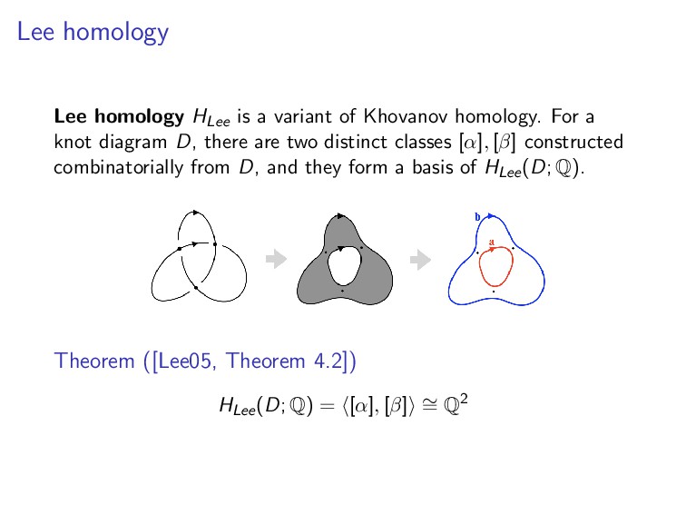
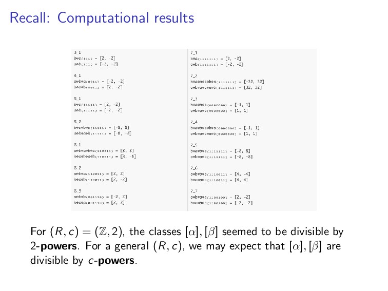
![Our observation Lee homology and the two classes [α], [β]](https://files.speakerdeck.com/presentations/1493326cd9024be9a12b9cdcd14fe52c/slide_10.jpg)
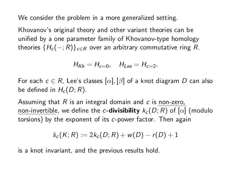
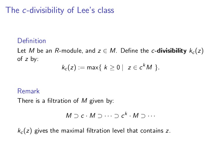
![Our results We define the 2-divisibility k2(D) of [α] (modulo](https://files.speakerdeck.com/presentations/1493326cd9024be9a12b9cdcd14fe52c/slide_13.jpg)
![Especially for (R, c) = (Q[h], h) we have the](https://files.speakerdeck.com/presentations/1493326cd9024be9a12b9cdcd14fe52c/slide_16.jpg)
![The canonical generator [ζ] for (R, c) = (Q[h], h)](https://files.speakerdeck.com/presentations/1493326cd9024be9a12b9cdcd14fe52c/slide_45.jpg)
![Proposition There is a unique class [ζ(D)] ∈ Hh(D; R)f](https://files.speakerdeck.com/presentations/1493326cd9024be9a12b9cdcd14fe52c/slide_46.jpg)
![The homomorphism property of sh Using the class [ζ], we](https://files.speakerdeck.com/presentations/1493326cd9024be9a12b9cdcd14fe52c/slide_47.jpg)
![Coincidence with the s-invariant Theorem (S.) sh(−; Q[h]) coincides with](https://files.speakerdeck.com/presentations/1493326cd9024be9a12b9cdcd14fe52c/slide_48.jpg)
![Proof continued. Denote by [α2], [αh] the α-classes of D](https://files.speakerdeck.com/presentations/1493326cd9024be9a12b9cdcd14fe52c/slide_49.jpg)
![Corollary s(K) = qdegh [ζ(K)] − 1. Remark The construction](https://files.speakerdeck.com/presentations/1493326cd9024be9a12b9cdcd14fe52c/slide_50.jpg)
![Question (2) Can we construct [ζ] ∈ Hc(D; R) for](https://files.speakerdeck.com/presentations/1493326cd9024be9a12b9cdcd14fe52c/slide_53.jpg)
![Question (3) Does s = sc(−; Q[h]) also hold for](https://files.speakerdeck.com/presentations/1493326cd9024be9a12b9cdcd14fe52c/slide_54.jpg)
![References I [BW08] A. Beliakova and S. Wehrli. “Categorification of](https://files.speakerdeck.com/presentations/1493326cd9024be9a12b9cdcd14fe52c/slide_56.jpg)
![References II [Ras10] J. Rasmussen. “Khovanov homology and the slice](https://files.speakerdeck.com/presentations/1493326cd9024be9a12b9cdcd14fe52c/slide_57.jpg)