Analyzing colony dynamics and visualizing cell diversity in spatiotemporal experiments

PhD defense given at Bielefeld University, Germany. May. 14, 2018.

Transcript

1. Analyzing colony dynamics and visualizing cell diversity in spatiotemporal experiments Georges Hattab Faculty of Technology, Bielefeld University
 14/05/2018 1 Courtesy of E. Ben-Jacob
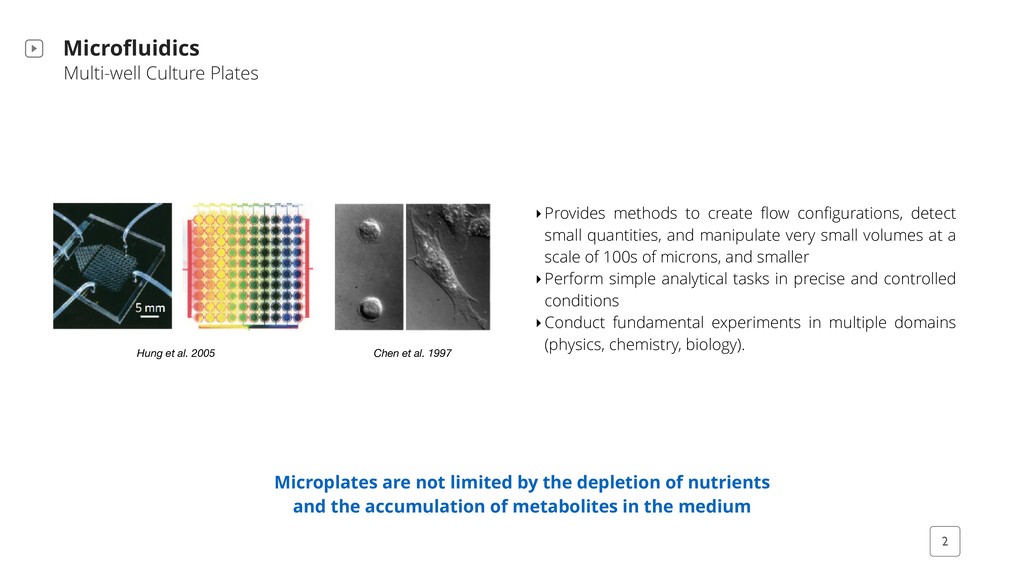
2. Microfluidics Multi-well Culture Plates 2 Microplates are not limited by the depletion of nutrients 
 and the accumulation of metabolites in the medium Chen et al. 1997 Hung et al. 2005 ‣Provides methods to create flow configurations, detect small quantities, and manipulate very small volumes at a scale of 100s of microns, and smaller ‣Perform simple analytical tasks in precise and controlled conditions ‣Conduct fundamental experiments in multiple domains (physics, chemistry, biology).
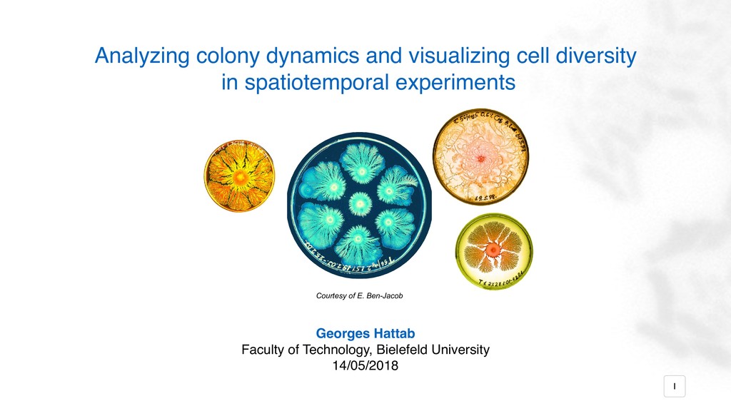
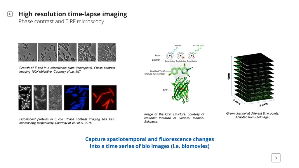
3. High resolution time-lapse imaging Phase contrast and TIRF microscopy 3 Capture spatiotemporal and fluorescence changes into a time series of bio images (i.e. biomovies) Growth of E coli in a microfluidic plate (microplate). Phase contrast imaging 100X objective. Courtesy of Lu, MIT Fluorescent proteins in E coli. Phase contrast imaging and TIRF microscopy, respectively. Courtesy of Wu et al. 2015. Green channel at different time points. Adapted from BioImageL time Image of the GFP structure. courtesy of National Institute of General Medical Sciences.
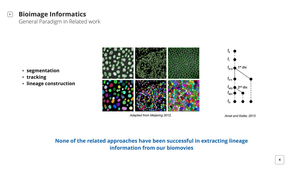
4. Bioimage Informatics General Paradigm in Related work 4 None of the related approaches have been successful in extracting lineage information from our biomovies Amat and Keller, 2013 ‣ segmentation ‣ tracking ‣ lineage construction Adapted from Meijering 2012. CELL SEGMENTATION: 50 YEARS DOWN THE ROAD 4 A B C D FIGURE 2: Examples of cell image segmentation based on the discussed approaches. The rows show, re- spectively, the input images, the automatically found cell contours (overlaid in green), and the correspond- ing labeled cell regions (arbitrary colors). (A) Cells that are fairly well separated and clearly brighter than the background are easily segmented using thresholding. Binary ultimate erosion and reconstruction was used to split the few clumped cells. (B) Scenarios with higher cell densities and intensity variations require more sophisticated methods. The method used here involves graph-cuts based binarization, Laplacian-of- Gaussian based cell detection (see red dots), and marker based clustering (from [14] with permission). (C) Membrane stained images are ideally suited for watershed based segmentation. Grayscale morphological prefiltering was used both for background estimation (opening operation) and filling imperfectly stained segments (closing operation). (D) Studies of intracellular dynamic processes often result in images with significant intensity variations (in both space and time) and require robust cell segmentation and tracking methods. The method used here is based on level sets [15]. All of these methods were specifically designed for the given application and required careful parameter tuning.
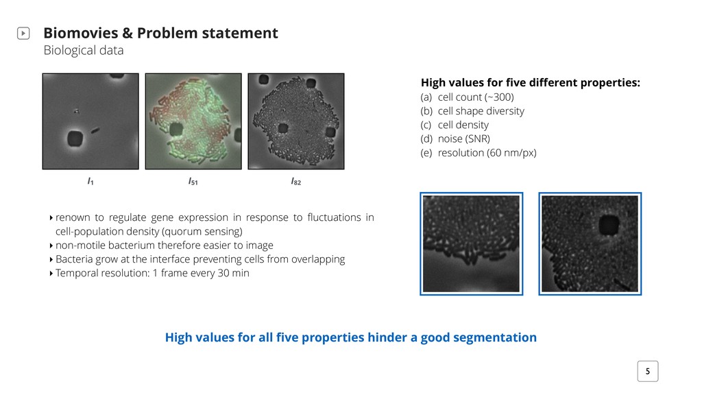
5. Biomovies & Problem statement Biological data 5 ‣ renown to regulate gene expression in response to fluctuations in cell-population density (quorum sensing) ‣ non-motile bacterium therefore easier to image ‣ Bacteria grow at the interface preventing cells from overlapping ‣ Temporal resolution: 1 frame every 30 min High values for all five properties hinder a good segmentation High values for five different properties: (a) cell count (~300) (b) cell shape diversity (c) cell density (d) noise (SNR) (e) resolution (60 nm/px) I 1 I 82 I 51
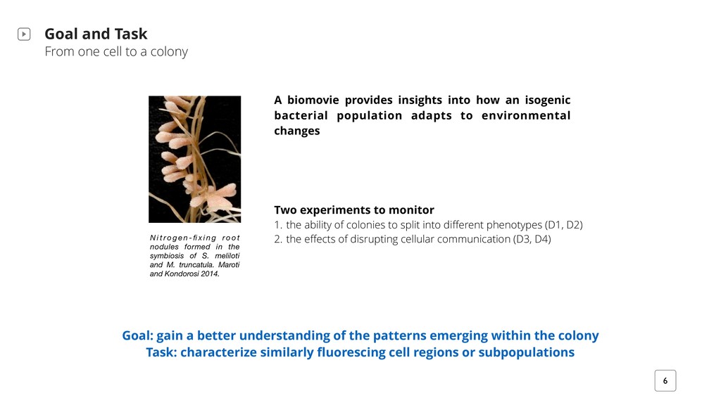
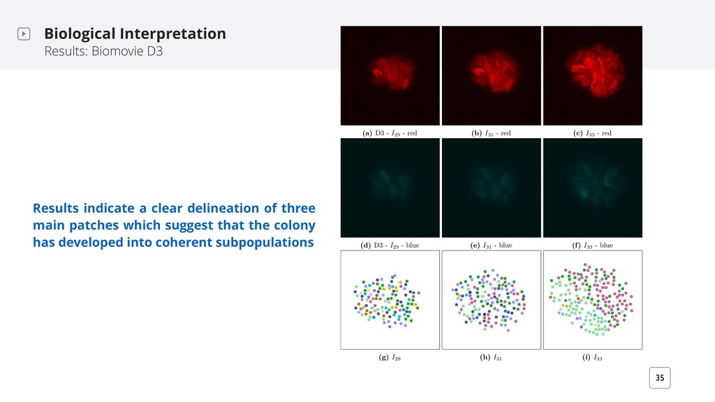
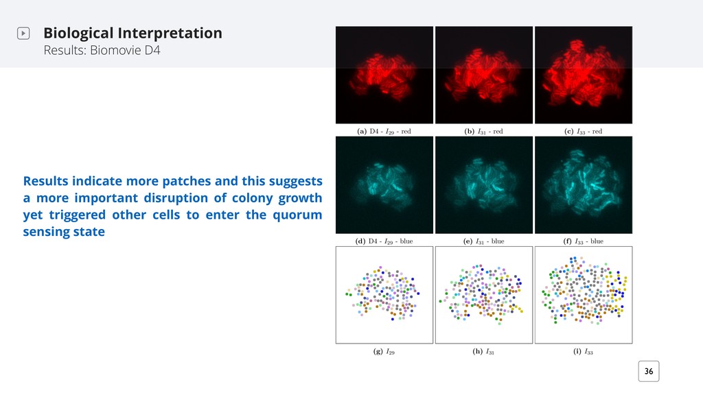
6. 6 Goal and Task From one cell to a colony Goal: gain a better understanding of the patterns emerging within the colony Task: characterize similarly fluorescing cell regions or subpopulations N i t r o g e n - fi x i n g r o o t nodules formed in the symbiosis of S. meliloti and M. truncatula. Maroti and Kondorosi 2014. A biomovie provides insights into how an isogenic bacterial population adapts to environmental changes Two experiments to monitor 1. the ability of colonies to split into different phenotypes (D1, D2) 2. the effects of disrupting cellular communication (D3, D4)
7. Overview I. Image registration 
 Correcting spatial shift is a prerequisite for posterior analyses II. Analytical approach 
 Extracting coherent lineages from biomovies 7
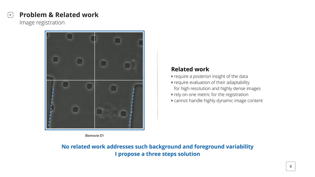
8. Problem & Related work Image registration 8 Related work ‣ require a posteriori insight of the data ‣ require evaluation of their adaptability
 for high resolution and highly dense images ‣ rely on one metric for the registration ‣ cannot handle highly dynamic image content Biomovie D1 No related work addresses such background and foreground variability I propose a three steps solution
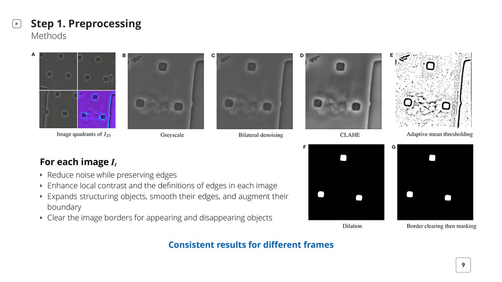
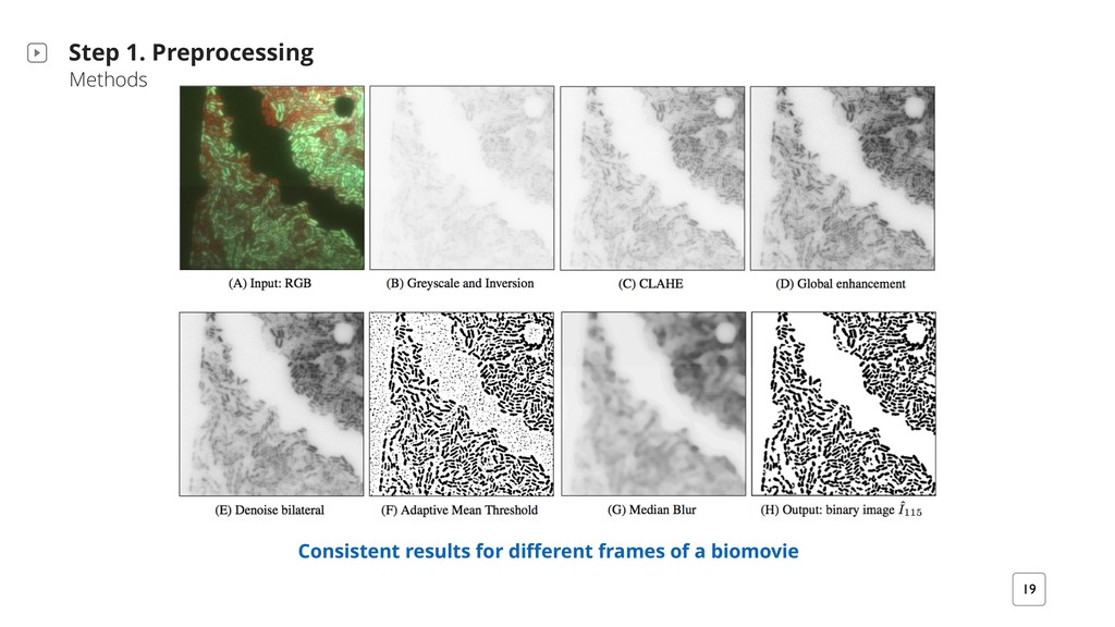
9. Step 1. Preprocessing Methods 9 Consistent results for different frames For each image It ‣ Reduce noise while preserving edges ‣ Enhance local contrast and the definitions of edges in each image ‣ Expands structuring objects, smooth their edges, and augment their boundary ‣ Clear the image borders for appearing and disappearing objects
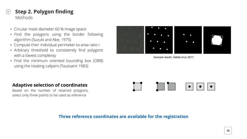
10. Step 2. Polygon finding Methods 10 Three reference coordinates are available for the registration Example results. Hattab et al. 2017. ‣ Circular mask diameter 60 % image space ‣ Find the polygons using the border following algorithm (Suzuki and Abe, 1975) ‣ Compute their individual perimeter-to-area ratio r ‣ Arbitrary threshold to consistently find polygons with a lowest complexity ‣ Find the minimum oriented bounding box (OBB) using the rotating calipers (Toussaint 1983) Adaptive selection of coordinates
 Based on the number of retained polygons, select only three points to be used as reference
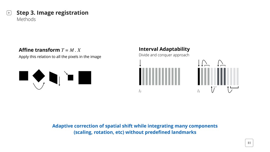
11. Interval Adaptability Divide and conquer approach I1 I1 [ [ [ [ Step 3. Image registration Methods 11 Adaptive correction of spatial shift while integrating many components (scaling, rotation, etc) without predefined landmarks Affine transform T = M . X Apply this relation to all the pixels in the image
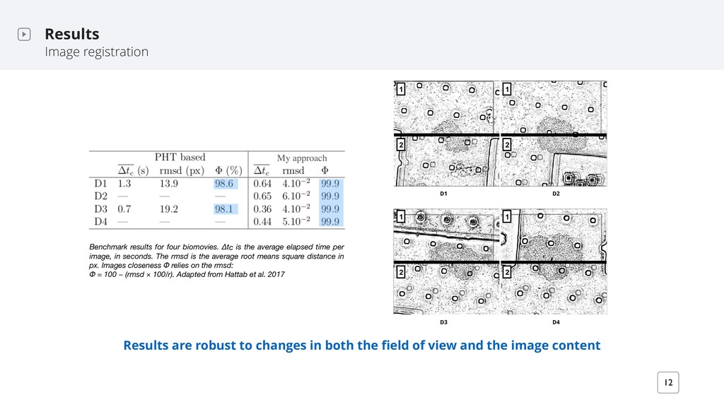
12. 12 Results Image registration Benchmark results for four biomovies. ∆tc is the average elapsed time per image, in seconds. The rmsd is the average root means square distance in px. Images closeness Φ relies on the rmsd:
 Φ = 100 − (rmsd × 100/r). Adapted from Hattab et al. 2017 Results are robust to changes in both the field of view and the image content D1 1 1 2 2 1 1 2 2 D2 D3 D4 My approach
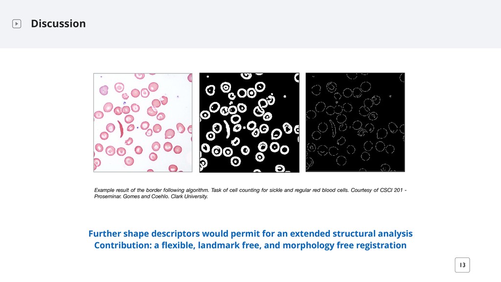
13. Example result of the border following algorithm. Task of cell counting for sickle and regular red blood cells. Courtesy of CSCI 201 - Proseminar. Gomes and Coehlo. Clark University. Discussion 13 Further shape descriptors would permit for an extended structural analysis
 Contribution: a flexible, landmark free, and morphology free registration
14. 5. Overview II. Analytical approach
 Extracting coherent lineages from biomovies 14 I. Image registration 
 Correcting spatial shift is a prerequisite for posterior analyses
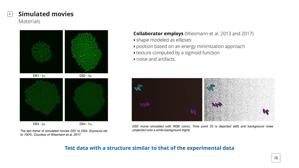
15. Simulated movies Materials 15 Test data with a structure similar to that of the experimental data The last frame of simulated movies DS1 to DS4. Exposure set to 100%. Courtesy of Wiesmann et al. 2017. Collaborator employs (Wiesmann et al. 2013 and 2017) ‣shape modeled as ellipses ‣position based on an energy minimization approach ‣texture computed by a sigmoid function ‣noise and artifacts. DS1 - I25 DS2 - I60 DS4 - I78 DS3 - I63 DS5 movie simulated with RGB colors. Time point 23 is depicted (left) and background noise projected onto a white background (right).
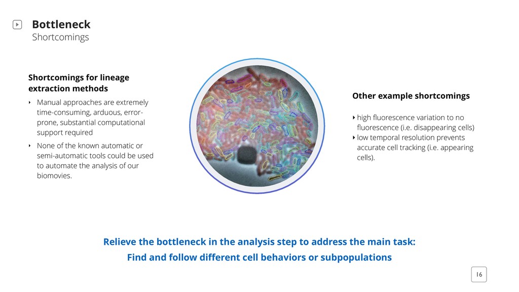
16. Bottleneck Shortcomings 16 Other example shortcomings ‣ high fluorescence variation to no fluorescence (i.e. disappearing cells) ‣ low temporal resolution prevents accurate cell tracking (i.e. appearing cells). Shortcomings for lineage extraction methods ‣ Manual approaches are extremely time-consuming, arduous, error- prone, substantial computational support required ‣ None of the known automatic or semi-automatic tools could be used to automate the analysis of our biomovies. Relieve the bottleneck in the analysis step to address the main task: Find and follow different cell behaviors or subpopulations
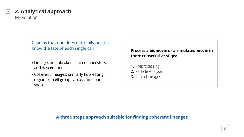
17. 2. Analytical approach My solution 17 Claim is that one does not really need to know the fate of each single cell ‣Lineage: an unbroken chain of ancestors and descendants ‣Coherent lineages: similarly fluorescing regions or cell groups across time and space A three steps approach suitable for finding coherent lineages Process a biomovie or a simulated movie in three consecutive steps: 1. Preprocessing 2. Particle Analysis 3. Patch Lineages
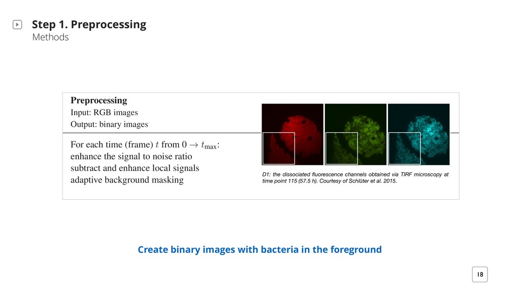
18. Step 1. Preprocessing Methods 18 Create binary images with bacteria in the foreground Hattab et al. Supplementary Material Preprocessing Input: RGB images Output: binary images For each time (frame) t from 0 ! tmax: preprocess() enhance the signal to noise ratio subtract and enhance local signals adaptive background masking Particles Input: binary images Output: particle trajectories For each get_data() time point: particle finding, and tracking trajectory: trajectory linking D1: the dissociated fluorescence channels obtained via TIRF microscopy at time point 115 (57.5 h). Courtesy of Schlüter et al. 2015.
19. 19 Step 1. Preprocessing Methods Consistent results for different frames of a biomovie
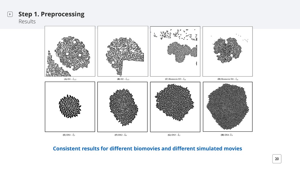
20. Step 1. Preprocessing Results 20 Consistent results for different biomovies and different simulated movies Hattab et al. Supplementary Material (A) D1 - ˆ I115 (B) D2 - ˆ I115 (C) Biomovie D3 - ˆ I44 (D) Biomovie D4 - ˆ I44 Figure S4. Binary images after preprocessing of the original biomovie final frames (D1–D4). (A) Biomovie D1 shows a phenotypic heterogeneity experiment, with two separate colonies visible. (B) Biomovie D2 is an alternate condition of the same experiment. (C) Biomovie D3 shows an experiment on bacterial communication by quorum sensing. (D) Biomovie D4 is an alternate condition of the same experiment. (A) D1 - ˆ I115 (B) D2 - ˆ I115 (C) Biomovie D3 - ˆ I44 (D) Biomovie D4 - ˆ I44 Figure S4. Binary images after preprocessing of the original biomovie final frames (D1–D4). (A) Biomovie D1 shows a phenotypic heterogeneity experiment, with two separate colonies visible. (B) Biomovie D2 is an alternate condition of the same experiment. (C) Biomovie D3 shows an experiment on bacterial communication by quorum sensing. (D) Biomovie D4 is an alternate condition of the same experiment. 8 (E) DS1 - Î25 (F) DS2 - Î60 (G) DS3 - Î63 (H) DS4- Î78
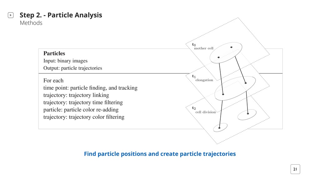
21. Output: binary images For each time (frame) t from 0 ! tmax: preprocess() enhance the signal to noise ratio subtract and enhance local signals adaptive background masking Particles Input: binary images Output: particle trajectories For each get_data() time point: particle finding, and tracking trajectory: trajectory linking trajectory: trajectory time filtering particle: particle color re-adding trajectory: trajectory color filtering Patch Lineages Input: particle trajectories Output: patch lineages graph (.gml or .json) At time tmax: modalgo() 1 - find patches 21 Find particle positions and create particle trajectories Step 2. - Particle Analysis Methods Hattab et al. Supplementary Material t2 cell division t1 elongation t0 mother cell (A) Single-cell segmentation (centroids) t2 cell division t1 elongation t0 mother cell (B) CYCASP approach (particles) Figure S1. Comparative illustration of single-cell segmentation approach to our particle-based solution for constructing lineages in biomovies. (A) Single-cell segmentation is used to track object centroids, detecting cell mitosis explicitly, and constructing cell lineages accordingly. (B) Multiple particles are detected within regions, and tracked over time, detecting mitosis implicitly.
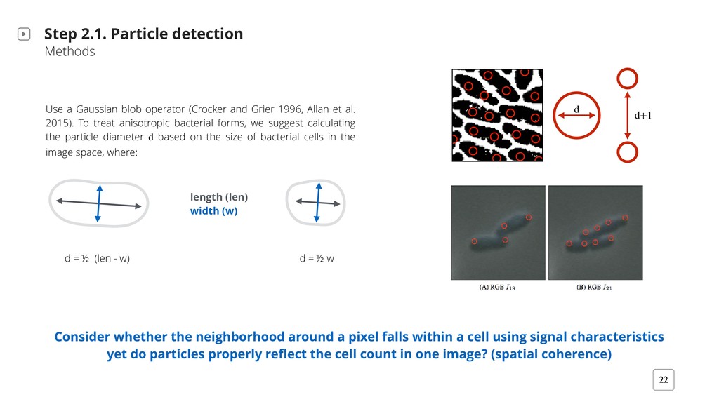
22. Step 2.1. Particle detection Methods 22 Use a Gaussian blob operator (Crocker and Grier 1996, Allan et al. 2015). To treat anisotropic bacterial forms, we suggest calculating the particle diameter d based on the size of bacterial cells in the image space, where: Consider whether the neighborhood around a pixel falls within a cell using signal characteristics
 yet do particles properly reflect the cell count in one image? (spatial coherence) Image portion ˆ I57.5: d = 9px (D) Image portion ˆ I31.5: d = 17px ary images annotated with computed particle positions (shown as red circles). (A) ovie D1 binary image. (B) Simulated movie binary image. (C) Original biomovie crop of 2 particles detected within each cell. A particle diameter value of d = 9px yields no false d d+1 length (len) width (w) d = ½ (len - w) d = ½ w
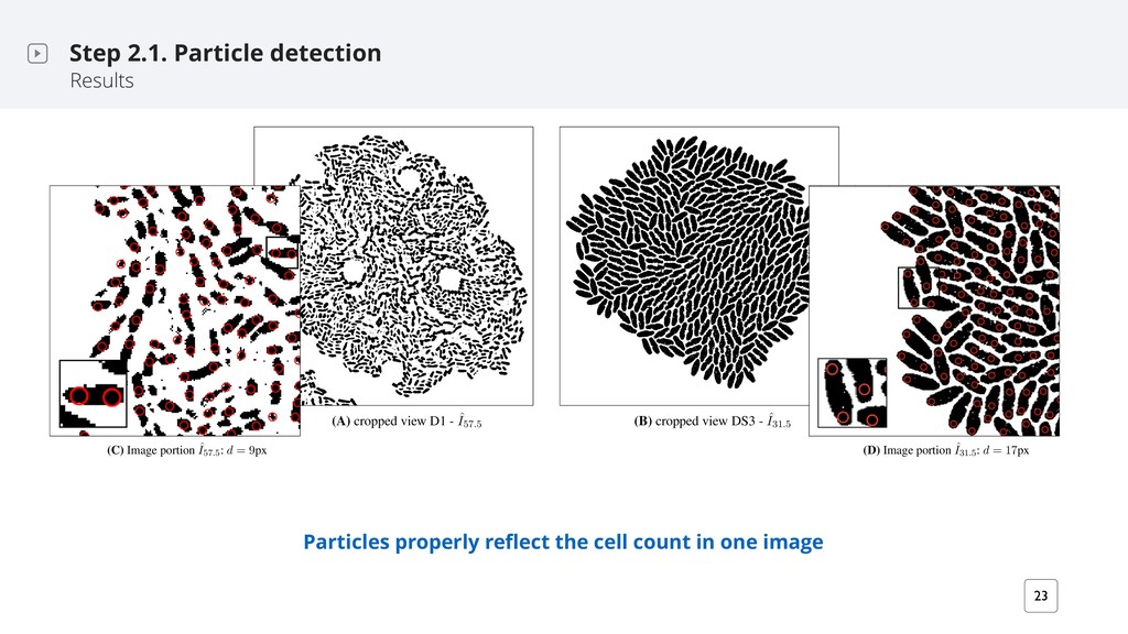
23. Step 2.1. Particle detection Results 23 Hattab et al. Method for the study of time-lapse image data (A) cropped view D1 - ˆ I57.5 (B) cropped view DS3 - ˆ I31.5 (A) cropped view D1 - ˆ I57.5 (B) cropped view DS3 - ˆ I31.5 (C) Image portion ˆ I57.5: d = 9px (D) Image portion ˆ I31.5: d = 17px Figure 2. Binary images annotated with computed particle positions (shown as red circles). (A) Original biomovie D1 binary image. (B) Simulated movie binary image. (C) Original biomovie crop of D1 showing 1-2 particles detected within each cell. A particle diameter value of d = 9px yields no false negatives, and some false positives that will be eliminated in subsequent processing that exploits temporal coherence. (D) Simulated movie crop showing ⇠2 particles detected per cell, with a particle diameter d = 17px. (A) cropped view D1 - ˆ I57.5 (B) cropped view DS3 - ˆ I31.5 (C) Image portion ˆ I57.5: d = 9px (D) Image portion ˆ I31.5: d = 17px Figure 2. Binary images annotated with computed particle positions (shown as red circles). (A) Original biomovie D1 binary image. (B) Simulated movie binary image. (C) Original biomovie crop of D1 showing 1-2 particles detected within each cell. A particle diameter value of d = 9px yields no false negatives, and some false positives that will be eliminated in subsequent processing that exploits temporal coherence. (D) Simulated movie crop showing ⇠2 particles detected per cell, with a particle diameter d = 17px. Particles properly reflect the cell count in one image
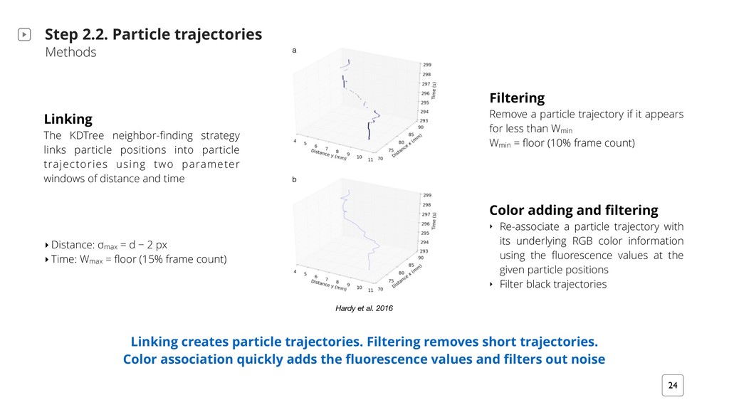
24. Step 2.2. Particle trajectories Methods 24 Linking creates particle trajectories. Filtering removes short trajectories. 
 Color association quickly adds the fluorescence values and filters out noise Linking The KDTree neighbor-finding strategy links particle positions into particle trajectories using two parameter windows of distance and time Filtering Remove a particle trajectory if it appears for less than Wmin Wmin = floor (10% frame count) Color adding and filtering ‣ Re-associate a particle trajectory with its underlying RGB color information using the fluorescence values at the given particle positions ‣ Filter black trajectories ‣ Distance: σ max = d − 2 px ‣ Time: Wmax = floor (15% frame count) Hardy et al. 2016
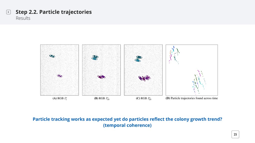
25. 25 Particle tracking works as expected yet do particles reflect the colony growth trend? 
 (temporal coherence) Step 2.2. Particle trajectories Results (A) RGB I? 1 (B) RGB I? 10 (C) RGB I? 20 (D) Particle trajectories found across time: t1–t23 Figure S11. Example result of particle linking for simulated biomovie DS5. The result is shown for cropped 375x500 px subsets of the original 2048x2048 px images depicting four to seven cells appearing in: cyan (top), and magenta (bottom) in (A–C). The black background was replaced by white pixels to better notice the cells. The threshold for particle finding was diameter d = 13 px and for particle linking the time filtering window was set to 3 frames. Computed particle locations annotated as 10 px white dots in (A–C). (A) Time point 1 shows two ancestor cells. (B) By time point 10 both ancestors have divided once. (C) By time point 20 the upper cyan colony has 3 cells, and the lower purple one has 4. (D) Particle trajectories covering the first 23 time points are shown by color coding each particle differently according the unique ID of the computed particle trajectory. This image crop contains 19 unique trajectories, all of which show an overall downward drift. For the entire DS5 biomovie, we globally found 383 particle positions resulting in 63 unique trajectories after linking, reduced to 34 trajectories after time filtering. (A) RGB I? 1 (B) RGB I? 10 (C) RGB I? 20 (A) RGB I? 1 (B) RGB I? 10 (C) RGB I? 20 (D) Particle trajectories found across time: t1–t23 Figure S11. Example result of particle linking for simulated biomovie DS5. The result is sh cropped 375x500 px subsets of the original 2048x2048 px images depicting four to seven cells a in: cyan (top), and magenta (bottom) in (A–C). The black background was replaced by white better notice the cells. The threshold for particle finding was diameter d = 13 px and for particl the time filtering window was set to 3 frames. Computed particle locations annotated as 10 px w in (A–C). (A) Time point 1 shows two ancestor cells. (B) By time point 10 both ancestors have once. (C) By time point 20 the upper cyan colony has 3 cells, and the lower purple one has 4. (D trajectories covering the first 23 time points are shown by color coding each particle differently a the unique ID of the computed particle trajectory. This image crop contains 19 unique traject of which show an overall downward drift. For the entire DS5 biomovie, we globally found 383 positions resulting in 63 unique trajectories after linking, reduced to 34 trajectories after time filt
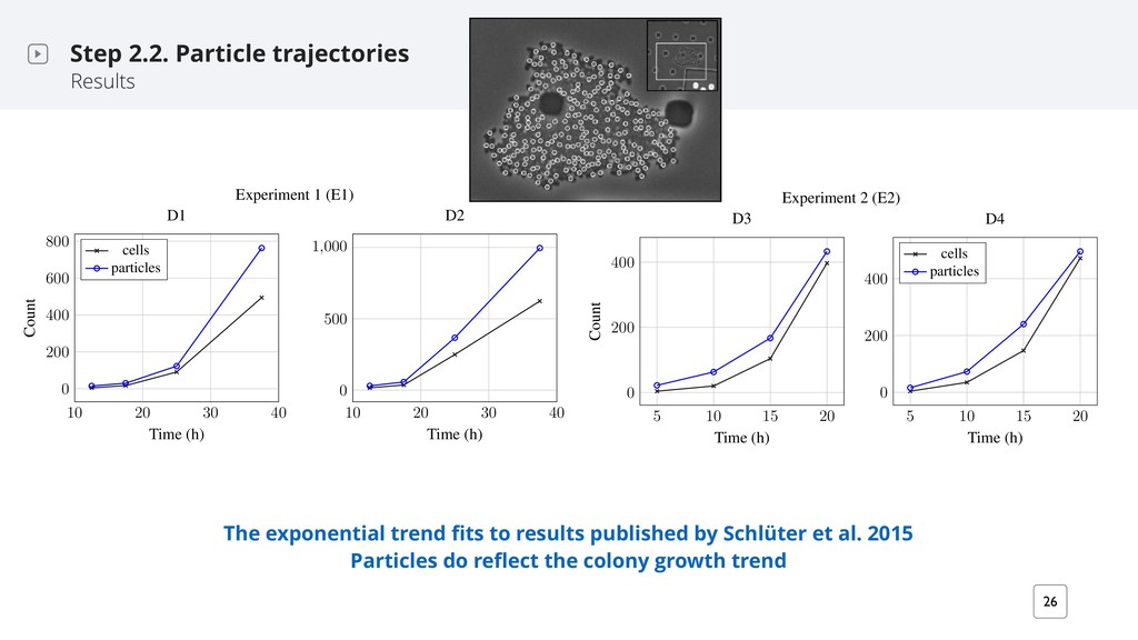
26. 26 The exponential trend fits to results published by Schlüter et al. 2015
 Particles do reflect the colony growth trend Step 2.2. Particle trajectories Results e S16. Comparison of the number of annotated cells to the number of computed particles our different time points for each biomovie. Observable cells were annotated using BIIGLE Langenk¨ amper et al. 2017). The four time points in E1 were selected before the colonies grew the image space (i.e. D2) or right before another colony invaded the image space (i.e. D1). The oyed parameters for both experiments are: max = 7 px, Wmax = 5 frames. The particle diameter 1 and E2 is set to 7 px and 9 px, respectively. The particle trend is consistent per experiment. On ge, we observe that there are at least 1.7 times more particles than there are cells. We calculated ssion models based on the number of particles in each experiment: E1 based on 60 frames, and E2 frames. The trend fits to an exponential regression for both experiments. E1 results are consistent he exponential trend in the first 21h of the biomovies as shown in Schl¨ uter et al. 2015. We report lculated regression parameter results and the average ratio of particles to annotated cells in the table . Experiment 1 (E1) 10 20 30 40 0 200 400 600 800 Time (h) Count D1 cells particles 10 20 30 40 0 500 1,000 Time (h) D2 Experiment 2 (E2) 200 400 Count D3 200 400 D4 cells particles 10 20 30 40 0 200 400 Time (h) Count 10 20 30 40 0 500 Time (h) Experiment 2 (E2) 5 10 15 20 0 200 400 Time (h) Count D3 5 10 15 20 0 200 400 Time (h) D4 cells particles
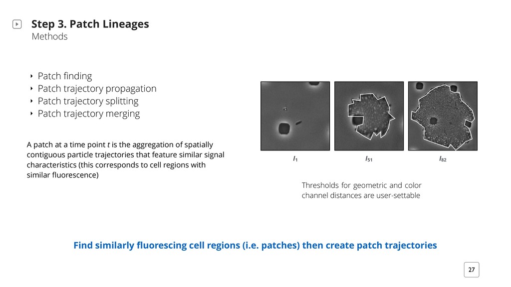
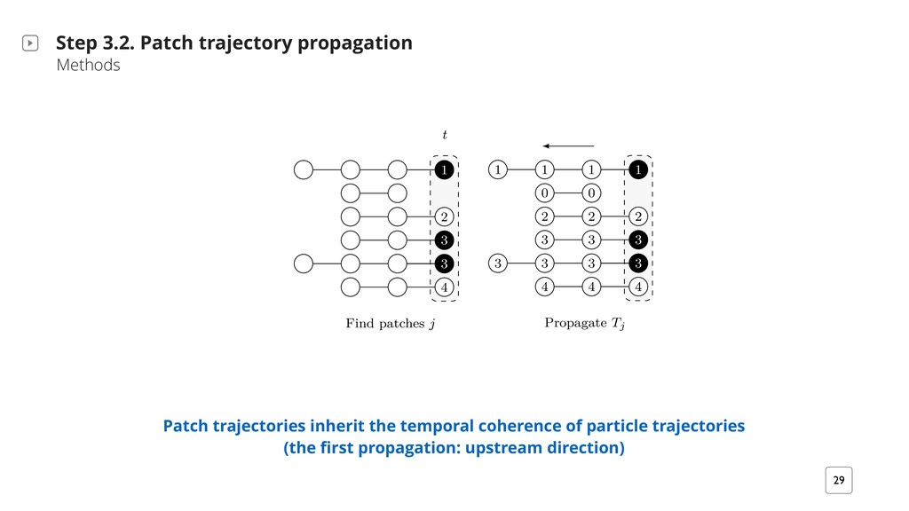
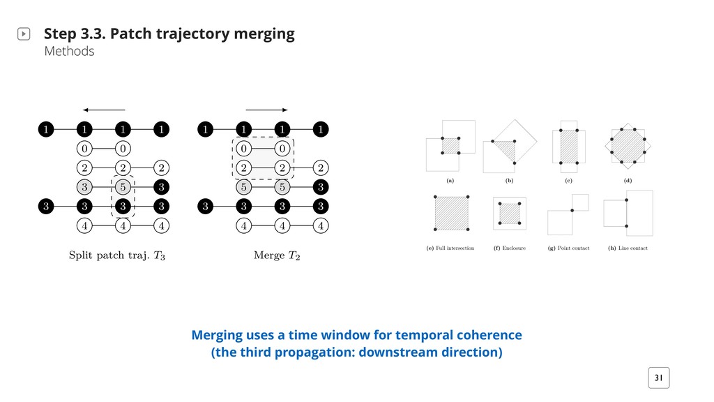
27. 27 Find similarly fluorescing cell regions (i.e. patches) then create patch trajectories Step 3. Patch Lineages Methods ‣ Patch finding ‣ Patch trajectory propagation ‣ Patch trajectory splitting ‣ Patch trajectory merging A patch at a time point t is the aggregation of spatially contiguous particle trajectories that feature similar signal characteristics (this corresponds to cell regions with similar fluorescence) I 1 I 82 I 51 Thresholds for geometric and color channel distances are user-settable
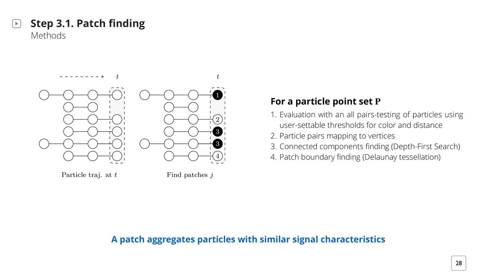
28. 28 Step 3.1. Patch finding Methods For a particle point set P 1. Evaluation with an all pairs-testing of particles using user-settable thresholds for color and distance 2. Particle pairs mapping to vertices 3. Connected components finding (Depth-First Search) 4. Patch boundary finding (Delaunay tessellation) i2/ QMiQ `Qrb r?2`2 iBK2 `mMb 7`QK H27i iQ `B;?iX S`iB+H2b `2 +QHQ`2/ r?Bi2- ;`2v- Q` +F iQ BHHmbi`i2 72im`2 bT+2 /Bz2`2M+2b- BX2X T`iB+H2 Q7 i?2 bK2 ;`2v pHm2 ?p2 bBKBH` im`2b UΦ(vt,p, vt,p′ ) = 1VX h?2 Ti+? HBM2;2 +QKTmiiBQM #2;BMb rBi? M BMBiBH Ti+? /BM; T`QT;iBQM i i?2 Hbi iBK2 TQBMi- b b?QrM BM 6B;X 8XkjUVX S`iB+H2b TB`b i?i Bb7v i?2 mb2` i?`2b?QH/b `2 ;`QmT2/ BMiQ 7Qm` Ti+?2b H#2HH2/ rBi? /BbiBM+i Ti+? A.b BM X 8XkjU#V- r?2`2 Ti+? j +QMiBMb irQ M2B;?#Q`BM; T`iB+H2b Q7 i?2 bK2 #H+F +QHQ`X UV S`iB+H2 i`DX i t i U#V 6BM/ Ti+?2b j i R k j j 9 m`2 8Xkj, :`T?B+H /2b+`BTiBQM BHHmbi`iBM; Ti+? }M/BM; BM i?2 }`bi bi2T Q7 i?2 Ti+? HBM2;2 bi`m+iBQM H;Q`Bi?KX 1+? `Qr b?Qrb  i2KTQ`HHv +Q?2`2Mi T`iB+H2 i`D2+iQ`v i?i Bb +HQb2 iQ i?Qb2 p2 M/ #2HQr Bi BM 72im`2 bT+2X h?2 /Qib `2T`2b2Mi T`iB+H2 TQbBiBQMb i 2+? iBK2 TQBMi M/ i?2B` Q`BM; Q7 r?Bi2f;`2vf#H+F `2T`2b2Mib /Bz2`2M+2b 7QmM/ BM 72im`2 bT+2 T`QpB/2/ i?2 mb2`@bT2+B}2/ 2b?QH/b- `2bT2+iBp2HvX h?2 bHB+2 Q7 bT+2@iBK2 i?i Bb i?2 7Q+mb Q7 +QKTmiiBQM BM 2+? bm#};m`2 Bb ?HB;?i2/ #v ;`2v #Qt2b rBi? /b?2/ QmiHBM2bX UV "BQKQpB2b ?p2  Mim`HHv Q++m``BM; i2KTQ`H 2+iBQM- `2T`2b2Mi2/ b  /b?2/ ``Qr 2M/BM; i iBK2 tX h?2 i`D2+iQ`B2b ?p2  /Bz2`2Mi MmK#2` Q7 iB+H2b- b?QrBM; i?i T`iB+H2b +M TT2` i Mv iBK2 TQBMiX U#V S`iB+H2 i`D2+iQ`B2b `2 ;`QmT2/ Q Ti+?2b i i?2 Hbi iBK2 TQBMiX 2 Ti+? }M/BM; K2i?Q/QHQ;v Bb /2b+`B#2/ BM 7Qm` KDQ` +QKTmiiBQMb /2b+`B#2/ BM /2iBH A patch aggregates particles with similar signal characteristics
29. 29 Patch trajectories inherit the temporal coherence of particle trajectories
 (the first propagation: upstream direction) Step 3.2. Patch trajectory propagation Methods Bb TTHB2/ iQ i?2 i2KTQ``v bm#;`T? UrBi? i?2 T`iB+H2 BM/2t b p2`iB+2bVX h?2 `2bmHi Bb mb2/ iQ p2`B7v i?i i?2 bm#;`T? Bb QM2 +QMM2+i2/ +QKTQM2MiX S`QpB/2/ i?2 bm#;`T?- i?2 +QMp2t ?mHH Bb +QKTmi2/- M/ Bib bBKTHB+2b `2 biQ`2/ BM  +QmMi2`+HQ+FrBb2 Q`/2`2/ HBbi- `2bT2+iBp2HvX h?2 2KTHQv2/ BKTH2K2MiiBQM `2HB2b QM i?2 ;`T? /i bi`m+im`2 M/ i?2 Qhull HB#``vRRjX h?2 HB#``v BM+Hm/2b i?2 +QKTmiiBQM Q7 i?2 .2HmMv i`BM;mHiBQM M/ i?2 +QMp2t ?mHHX UV 6BM/ Ti+?2b j i R k j j 9 U#V S`QT;i2 Tj R R R R y y k k k j j j j j j j 9 9 9 R k j j 9 6B;m`2 8Xke, :`T?B+H /2b+`BTiBQM BHHmbi`iBM; Ti+? i`D2+iQ`v }M/BM; M/ T`QT;iBQMX 1+? `Qr b?Qrb  i2KTQ`HHv +Q?2`2Mi T`iB+H2 i`D2+iQ`v i?i Bb +HQb2 iQ i?Qb2 #Qp2 M/ #2HQr Bi BM 72im`2 bT+2X h?2 /Qib `2T`2b2Mi T`iB+H2 TQbBiBQMb i 2+? iBK2 TQBMi M/ i?2B` +QHQ`BM; Q7 r?Bi2f;`2vf#H+F `2T`2b2Mib /Bz2`2M+2b 7QmM/ BM 72im`2 bT+2 T`QpB/2/ i?2 mb2`@bT2+B}2/ i?`2b?QH/b- `2bT2+iBp2HvX h?2 bHB+2 Q7 bT+2@iBK2 i?i Bb i?2 7Q+mb Q7 +QKTmiiBQM BM 2+? bm#};m`2 Bb ?B;?HB;?i2/ #v ;`2v #Qt2b rBi? /b?2/ QmiHBM2bX h?2 #H+F ``Qr BM/B+i2b i?2 /B`2+iBQM Q7  T`QT;iBQMX UV S`iB+H2 i`D2+iQ`B2b `2 ;`QmT2/ BMiQ Ti+?2b i i?2 Hbi iBK2 TQBMiX U#V h?2 i`D2+iQ`v BM7Q`KiBQM Bb T`QT;i2/ mTbi`2K BM  `mM 7`QK i?2 Hbi iQ i?2 }`bi iBK2 TQBMiX
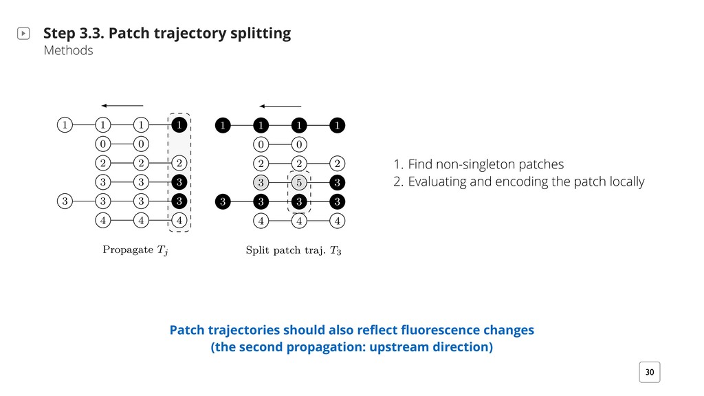
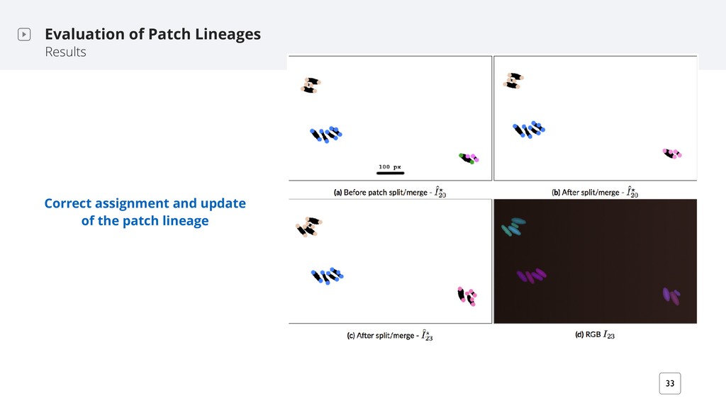
30. 30 Step 3.3. Patch trajectory splitting Methods TBM; HH MQM@bBM;H2iQM Ti+?2b M/ i?2B` T`iB+H2b QMiQ  i2KTQ``v ;`T? G X h?2M- i?2 a Bb TTHB2/ iQ }M/ +QMM2+i2/ +QKTQM2Mib BM G′X G2i S1 #2 i?2 }`bi Ti+? UQ` bm#;`T?V Q7 HH MQM@bBM;H2iQM bm#;`T?b {Sn} rBi? n4bm#@ T? BM/2tX G2i iv #2 i?2 MmK#2` Q7 p2`iB+2b BM i?2 +QMM2+i2/ +QKTQM2Mi i?i biBb7v i?2 rBM; +QM/BiBQM, iv > 1X UV S`QT;i2 Tj R R R R y y k k k j j j j j j j 9 9 9 R k j j 9 U#V aTHBi Ti+? i`DX T3 R R R R y y k k k j j j j j 9 9 9 8 j R k j 9 j m`2 8Xkd, :`T?B+H /2b+`BTiBQM BHHmbi`iBM; Ti+? i`D2+iQ`v T`QT;iBQM M/ bTHBiiBM;X h?2 #H+F r BM/B+i2b i?2 /B`2+iBQM Q7  T`QT;iBQMX UV h?2 i`D2+iQ`v BM7Q`KiBQM Bb T`QT;i2/ mTbi`2K `mM 7`QK i?2 Hbi iQ i?2 }`bi iBK2 TQBMiX U#V h?2 bTHBi T`QT;iBQM T`Q+22/b 7`QK i?2 Hbi iQ i?2 iBK2 TQBMiX i+? 2pHmiBQM M/ 2M+Q/BM; Patch trajectories should also reflect fluorescence changes
 (the second propagation: upstream direction) 1. Find non-singleton patches 2. Evaluating and encoding the patch locally
31. 31 Merging uses a time window for temporal coherence
 (the third propagation: downstream direction) Step 3.3. Patch trajectory merging Methods UV aTHBi Ti+? i`DX T3 R R R R y y k k k j j j j j 9 9 9 8 j R k j 9 j U#V J2`;2 T2 R R R R y y k k k j j j j j 9 9 9 8 8 R k j 9 j 8Xk3, :`T?B+H /2b+`BTiBQM BHHmbi`iBM; Ti+? i`D2+iQ`v bTHBiiBM; M/ K2`;BM;X 1+? `Qr i2KTQ`HHv +Q?2`2Mi T`iB+H2 i`D2+iQ`v i?i Bb +HQb2 iQ i?Qb2 #Qp2 M/ #2HQr Bi BM 72im`2 ?2 /Qib `2T`2b2Mi T`iB+H2 TQbBiBQMb i 2+? iBK2 TQBMi M/ i?2B` +QHQ`BM; Q7 r?Bi2f;`2vf#H+F ib /Bz2`2M+2b 7QmM/ BM 72im`2 bT+2 T`QpB/2/ i?2 mb2`@bT2+B}2/ i?`2b?QH/b- `2bT2+iBp2HvX h?2 T+2@iBK2 i?i Bb i?2 7Q+mb Q7 +QKTmiiBQM BM 2+? bm#};m`2 Bb ?B;?HB;?i2/ #v ;`2v #Qt2b rBi? miHBM2bX h?2 #H+F ``Qr BM/B+i2b i?2 /B`2+iBQM Q7  T`QT;iBQMX UV h?2 bTHBi T`QT;iBQM 7`QK i?2 Hbi iQ i?2 }`bi iBK2 TQBMiX U#V h?2 K2`;2 T`QT;iBQM T`Q+22/b 7`QK }`bi iQ i?2 TQBMi- KB``Q`BM; #BQHQ;B+H ;`Qri?X i bTiBHHv M/ Ti+? i`D2+iQ`v K2`;BM; r?B+? `2HB2b QM  mb2`@/2}M2/ K2`;2 rBM/Qr BMi2`b2+iBQM Bb 7QmM/ BM i?2 T`2pBQmb bi2T- i?2 .6a H;Q`Bi?K Bb TTHB2/ QM i?2 mMBQM Q7 i?2b2 bm#;`T?bX DFS(St1 ∪ St2) ⇔ St1′ U8XRkV qBi? St1′  +QMM2+i2/ +QKTQM2MiX A7 2[miBQM U8XRkV ?QH/b- i?2 Ti+? BM/B+2b `2 biQ`2/ BM  +M/B/i2 K2`;2 HBbi- 7Q`Kii2/ b (t (1,2))X 1Hb2- i?2 H;Q`Bi?K Bi2`i2b QMiQ i?2 M2ti TB` Q7 Ti+?2b i?i BMi2`b2+iX S`QpB/2/  mb2`@/2}M2/ K2`;2 rBM/Qr ωt - Ti+?2b i?i TT2` 7Q` i?2 H2M;i? Q7 i?i rBM/Qr `2 T`QT;i2/ i?`Qm;?Qmi i?2 K2`;2 rBM/QrX 6Q` BMbiM+2- T`QpB/2/ P1 M/ P2 M/  ;Bp2M K2`;2 rBM/Qr ωt = 5c bm+? b Ti+? R Bb H`;2` i?M Ti+? kX h?2M i?2 bm#b2i Q7 T`iB+H2 TQbBiBQMb BM P2 7Q` T`iB+H2 BM/2t R +M #2 r`Bii2M {(x, y)t=1,p=1,n=1, . . . , (x, y)t=5,p=1,n=1}X b /2TB+i2/ BM 6B;m`2 8Xjk- i?2 K2`;2 `2bmHib BM  `2bbB;MK2Mi Q7 i?2 Ti+? A.X Pi?2`rBb2- i?2 H;Q`Bi?K Bi2`i2b Qp2` i?2 M2ti UV U#V U+V U/V U2V 6mHH BMi2`b2+iBQM U7V 1M+HQbm`2 U;V SQBMi +QMi+i U?V GBM2 +QMi+i 6B;m`2 8Xjy, 1tKTH2 BHHmbi`iBQMb Q7 BMi2`b2+iBQM +QM};m`iBQMb 7Q` irQ KBMBKmK `2 `2+iM;H2bX h?2 i2tim`2/ Tii2`M BM/B+i2b i?2 BMi2`b2+iBM; `2;BQMX AMi2`b2+iBM; p2`iB+2b `2 BM/B+i2/ BM #H+FX UĜ /V *b2b Q7 T`iBH BMi2`b2+iBQMX U2V 6mHH BMi2`b2+iBQM- r?2`2 #Qi? `2+iM;H2b b?`2 i?2 bK2 p2`iB+2bX U7V PM2 `2+iM;H2 Bb 2M+HQb2/ BMiQ i?2 Qi?2`X U;V  TQBMi +QMi+i- r?2`2 irQ `2+iM;H2b b?`2 QM2 p2`i2tX U?V  HBM2 +QMi+i- r?2`2 irQ `2+iM;H2b b?`2 M 2/;2X 6B;m`2 /Ti2/ 7`QK PT2M*oX http://docs.opencv.org/ Nj
32. 32 Particle related computation time is related to the density of the colony Computational Performance Results .aR .a8 .j .9 .ak .aj .a9 .R .k 0 200 400 38.5 32.96 27.14 26.7 71 195.65 371 93.41 97.48 Uk8V UkeV U99V U99V UeyV UejV Ud3V URR8V URR8V "BQKQpB2b U7`K2 +QmMiV 1HTb2/ iBK2 UbV 6B;m`2 8XRd, 1HTb2/ iBK2 Q7 i?2 T`iB+H2 bi2T 7Q` HH #BQKQpB2b- BM b2+QM/b- BM+Hm/BM; HH i?`22 T?b2b Q7 T`iB+H2 }M/BM;- HBMFBM;- M/ }Hi2`BM;X "BQKQpB2b BM i?2 t@tBb `2 bQ`i2/ #v 7`K2 +QmMi- 7`QK HQr2bi iQ ?B;?2bi Ub BM/B+i2/ BM T`2Mi?2b2bVX A Q#b2`p2 i?i T`iB+H2@`2Hi2/ +QKTmiiBQM iBK2 Bb `2Hi2/ iQ i?2 /2MbBiv Q7 i?2 +QHQMv BM i?2 #BQKQpB2- `i?2` i?M i?2 MmK#2` Q7 7`K2bX h?2 .a9 #BQKQpB2 Bb  ?B;?Hv /2Mb2 bT2+BH +b2- r?2`2 }M/BM; M/ HBMFBM; BM iBK2 Qp2` dyyy T`iB+H2b iF2b Qp2` e KBMX h?2b2 T`Q+2/m`2b +M #2 +QKTmiiBQMHHv 2tT2MbBp2- ;Bp2M  ?B;?Hv TQTmHi2/ +QHQMv M/  T`iB+H2 /BK2i2` b2i iQ  HQr pHm2X amKK`v, h?2 T`iB+H2 /2i2+iBQM M/ T`iB+H2 i`D2+iQ`v +QMbi`m+iBQM bi2T bm++2bb7mHHv +T@ im`2b i?2 bTiBH M/ i2KTQ`H BM7Q`KiBQM BM i?2 #BM`v BK;2 b2[m2M+2 rBi?Qmi +QKTmiBM; 2tTHB+Bi BK;2 b2;K2MiiBQM i i?2 H2p2H Q7 BM/BpB/mH +2HHbX h?Bb TT`Q+? Bb +QKTmiiBQMHHv 2{+B2Mi M/ `2[mB`2b MQ KMmH BMi2`p2MiBQMX Ai Bb `Q#mbi iQ i?2 i`MbB2Mi BMi2`+iBQMb #2@ ir22M M2B;?#Q`BM; +2HHb i?i rQmH/ +mb2 KBb@b2;K2MiiBQM BM ii2KTib iQ /2i2+i BM/BpB/mH .aR .a8 .j .9 .ak .aj .a9 .R .k 0 20 40 60 6.25 9 18.86 19.6 15.6 16.46 42.96 52.59 53.79 Uk8V UkeV U99V U99V UeyV UejV Ud3V URR8V URR8V "BQKQpB2b U7`K2 +QmMiV 1HTb2/ iBK2 UbV 6B;m`2 8Xj, 1HTb2/ iBK2 Q7 i?2 T`2T`Q+2bbBM; bi2T 7Q` HH #BQKQpB2b- BM b2+QM/bX "BQKQpB2b BM i?2 t@tBb `2 bQ`i2/ #v 7`K2 +QmMi- 7`QK HQr2bi iQ ?B;?2bi Ub BM/B+i2/ BM T`2Mi?2b2bVX M TT`QtBKi2 +Q``2HiBQM #2ir22M 7`K2 +QmMi M/ T`2T`Q+2bbBM; iBK2 Bb MQiB+2#H2X 6B;m`2 8XRjUV b?Qrb i?2 `2bmHi Q7 i?2 T`2T`Q+2bbBM; iQ 2M?M+2 i?2 +2HH@#+F;`QmM/ +QMi`bi BM i?2 _:" BK;2b b?QrM BM 6B;X kXRU+Ĝ7V U7`K2 I115 Q7 .RVX q?2`2b- 2+? bi2T Q7 i?2 T`2T`Q+2bbBM; TBT2HBM2 7Q` i?2 }MH 7`K2 Q7 #BQKQpB2 .R Bb /2TB+i2/ BM 6B;m`2 8XNX h?2 }MH #BM`v BK;2 Q7 2+? #BQKQpB2 Bb b?Qr+b2/ BM i?2 7QHHQrBM; 6B;m`2b 8XRy Ĝ 8XRkX An approximate correlation between frame count and preprocessing time Preprocessing Particle Analysis
33. 33 Correct assignment and update of the patch lineage Evaluation of Patch Lineages Results
34. 34 This framework can automatically extract patch lineages in less than 5 min for biomovies containing more than 100 frames and 300 cells Parameter Space Results UV I33 , `2/ +?MM2H U2tTQbm`2 YeyWV U#V :`22M +?MM2H U2tTQbm`2 YNyW U+V "Hm2 +?MM2H U2tTQbm`2 YNyWV U/V /4jy- `4R8- ;48y- #4R8 U2V /4ey- `4jy- ;4Ryy- #4jy U7V /4Ryy- `4ky- ;48y- #48y U;V ;43y U?V `48y 6B;m`2 8Xj9, 1tKTH2 Q7 T`K2i2` imMBM; iQ 2KT?bBx2 /Bz2`2Mi +?MM2Hb- 7Q` iBK2 TQBMi jj Q7 #BQKQpB2 .jX h?2 #BM`v BK;2b BM i?2 #QiiQK `Qr `2 MMQii2/ rBi? N@Tt /Qib b?QrBM; T`iB+H2 HQ+iBQMb- +QHQ`2/ ++Q`/BM; iQ i?2B` Ti+? A.bX h?2 T`iB+H2 MHvbBb i?`2b?QH/b BM i?2 T`2pBQmb +QKTmiiBQMH bi2T r2`2 b2i iQ N Tt T`iB+H2 /BK2i2`-  8 Tt /BbiM+2 M/ Ry 7`K2 rBM/Qr 7Q` T`iB+H2 HBMFBM;- M/  j 7`K2 rBM/Qr 7Q` iBK2 }Hi2`BM;X UĜ+V a2T`i2 pB2rb Q7 `2/- ;`22M- M/ #Hm2 +?MM2Hb b?Qr i?2 ?B;? bi`m+im`H p`BiBQM #2ir22M 2+? +?MM2HX U/Ĝ7V h?`22 /Bz2`2Mi +QK#BMiBQMb Q7 b2iiBM;b
35. 35 Biological Interpretation Results: Biomovie D3 Results indicate a clear delineation of three main patches which suggest that the colony has developed into coherent subpopulations UV .j @ I29 @ `2/ U#V I31 @ `2/ U+V I33 @ `2/ U/V .j @ I29 @ #Hm2 U2V I31 @ #Hm2 U7V I33 @ #Hm2 U;V I29 U?V I31 UBV I33 6B;m`2 8Xj3, "BQKQpB2 .j rBi? _:" +?MM2Hb Q7 BK;2 TQBMib kN- jR M/ jj- M/ i?2B` +Q``2bTQM/BM; Ti+? bi`m+im`2- `2bT2+iBp2HvX 1M?M+2/ 2tTQbm`2b 7Q` `2/, eyW M/ #Hm2, NyWX h?2 aX K2HBHQiB #+i2`BH +2HHb `2 #BQ@2M;BM22`2/ iQ ~mQ`2b+2 BM  T`iB+mH` rv- r?2`2 2+? +?MM2H 2M+Q/2b  +2`iBM i`Bi Q` #2?pBQ`X h?2 `2/ UĜ+V M/ #Hm2 +?MM2Hb U/Ĝ7V b?Qr +2`iBM #2?pBQ` BM `2bTQMb2 iQ +?M;2b
36. UV .9 @ I29 @ `2/ U#V I31 @ `2/ U+V I33 @ `2/ U/V .9 @ I29 @ #Hm2 U2V I31 @ #Hm2 U7V I33 @ #Hm2 U;V I29 U?V I31 UBV I33 6B;m`2 8XjN, "BQKQpB2 .9 rBi? _:" +?MM2Hb Q7 BK;2 TQBMib kN- jR M/ jj- M/ i?2B` +Q``2bTQM/BM; Ti+? bi`m+im`2- `2bT2+iBp2HvX 1M?M+2/ 2tTQbm`2b 7Q` i?2 #Hm2 +?MM2H, NyWX b b22M BM 6B;X 8Xj3- i?2 #BQKQpB2 b?Qr+b2b #BQ@2M;BM22`2/ aX K2HBHQiB #+i2`BH +2HHb ~mQ`2b+BM; BM  T`iB+mH` rv, h?2 `2/ UĜ+V M/ #Hm2 +?MM2Hb U/Ĝ7V b?Qr +2`iBM #2?pBQ` BM `2bTQMb2 iQ +?M;2b Q7 +QM/BiBQMbc ?2`2 i?2 36 Biological Interpretation Results: Biomovie D4 Results indicate more patches and this suggests a more important disruption of colony growth yet triggered other cells to enter the quorum sensing state
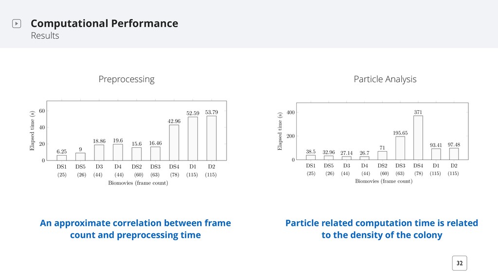
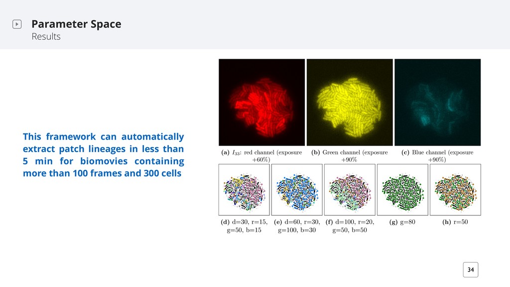
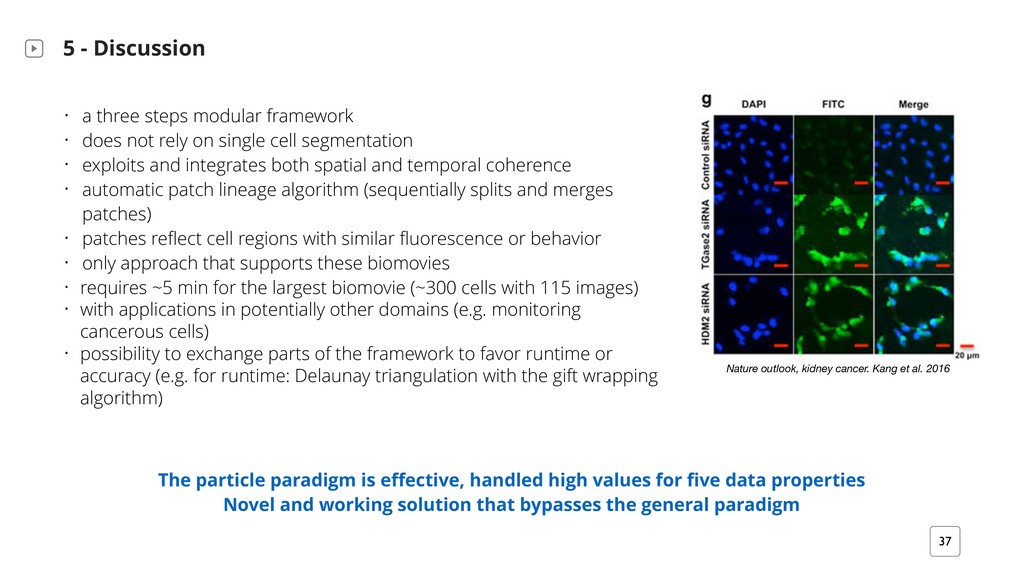
37. 5 - Discussion 37 • a three steps modular framework • does not rely on single cell segmentation • exploits and integrates both spatial and temporal coherence • automatic patch lineage algorithm (sequentially splits and merges patches) • patches reflect cell regions with similar fluorescence or behavior • only approach that supports these biomovies • requires ~5 min for the largest biomovie (~300 cells with 115 images) • with applications in potentially other domains (e.g. monitoring cancerous cells) • possibility to exchange parts of the framework to favor runtime or accuracy (e.g. for runtime: Delaunay triangulation with the gift wrapping algorithm) Nature outlook, kidney cancer. Kang et al. 2016 The particle paradigm is effective, handled high values for five data properties
 Novel and working solution that bypasses the general paradigm
38. Availability Open source https://goo.gl/ddAVS2 Open Data 
 
 Image registration 
 38 Analytical approach 

39. Publications Journals 2018 | Journal Article 3D space-time cube rendering for visualization of microfluidics image data Hattab G, Nattkemper TW (2018) Currently under revision Oxford Bioinformatics 2018 | Journal Article A Novel methodology for characterizing cell subpopulations in automated time-lapse microscopy Hattab G, Wiesmann V, Becker A, Munzner T, Nattkemper TW (2018) Frontiers in Bioengineering and Biotechnology 6: 17. 2017 | Journal Article ViCAR: An Adaptive and Landmark-Free Registration of Time Lapse Image Data from Microfluidics Experiments Hattab G, Schlüter J-P, Becker A, Nattkemper TW (2017) Frontiers in Genetics 8: 69. Conference 2016 | Information+ conference A mnemonic card game for your amino acids Hattab G, Brink B, Nattkemper TW (2016) Vancouver, Canada 39 Data Wiesmann V, Bergler M, Münzenmayer C, Wittenberg T (2017) : Fraunhofer Institute for Integrated Circuits, Erlangen, Germany. doi:10.4119/unibi/2915541. McIntosh M, Bettenworth V (2017) : Philipps University of Marburg. doi:10.4119/unibi/2913120. Schlueter J-P, McIntosh M, Hattab G, Nattkemper TW, Becker A (2015) : Bielefeld University. doi:10.4119/unibi/2777409.
40. Acknowledgments Prof. Tim W Nattkemper Prof. Anke Becker Prof. Tamara Munzner Veit Wiesmann Jan-Phillip Schlüter
 Dr. Matthew McIntosh 40