Survival Analysis in R and Python

PyData London 2016 talk.

Transcript

1. 1 Survival Analysis in R and Python @lindauruchurtu
2. 2 about me
3. Linda Physicist I like my space stringy rather than loopy Data Science From on-demand cabs to fashion Elsewhere Ballet / Books / Drawing / Photography Python since Late 2012 3
4. 4 intro
5. 5 https://xkcd.com/881/ http://www.xkcd.com/881/
6. Survival analysis is given to the name of statistical techniques that have to do with analysing the timing of events (duration data) and its relationship with covariates. 6 Traditionally, medical researchers and actuaries have dealt with the type of questions addressed by Survival Analysis: • What is the expected lifetime of patients given treatment A? • What is the life expectancy in London? It is also widely used in engineering to look at failure in mechanical systems (reliability theory). survival analysis
7. But survival techniques have many applications in the industry 7 • What is the time between signup and first order/use? • When will a customer churn? • How long before a tweet has no effect? • When will a store run out of product? • How long before person replaces his/her phone? • How long is the career of a football player? • What is the expected lifetime of a Stark? motivation At lyst: Prediction of Out of Stock products.
8. 8 You’ll hear a lot about lyst elsewhere… instead…
9. 9 • Argue that survival analysis is a very useful set of techniques that can be used as part of a standard data science pipeline - acquiring/cleaning/storing/ modelling • Expand on techniques to evaluate survival functions via random forests and
 generalised additive models.
 • Keep advocating the use of Python or R according to the use case in hand • Show it explicitly by applying it to a real dataset…. this talk
10. 10 Academic Careers!! What is the average lifetime of an academic career?
11. 11 http://www.phdcomics.com/comics/archive_print.php?comicid=1212
12. 12 survival 101
13. definitions 13 Birth Event: Time associated with the beginning of an observation period. Death Event: Time associated with the end of the observation period either by an event, end of the study or withdrawal from it. Censorship: We don’t always see the death event occur. The current time or other events, censor us from seeing the death event.
15. 15 survival function Describes the probability that the system will survive beyond a time t The survival time T may be thought of as a random variable. S(t) = P({T > t})
16. and p is the distribution of lifetimes. The hazard rate as a function of the survival function is called the hazard function. When the hazard is constant, survival time is described by the exponential distribution. Integrating the hazard function from 0 to t yields the cumulative hazard function: The instantaneous hazard rate describes the probability that the event T occurs in t+ , given that the individual is alive at t: 16 hazard function when (t) = p(t) S(t) (t) = lim t 0 Pr(t T<t+ t|T>t) t t t 0 (t) = t 0 (x)dx = log S(t)
17. where is the risk set at time and is the number of observations from the random event whose distribution we are trying to estimate. 17 Kaplan-Meier Estimator It is a non-parametric maximum likelihood estimate of the survival function. It is a step function with jumps at observed event times. S(t) = j−1 i=1 1 − si ri tj−1 ≤ t < tj ri ti si Nelson-Aalen Estimator We can also given a non-parametric estimate of the cumulative hazard function: H(t) = j−1 i−1 si ri tj−1 ≤ t < tj
18. 18 surviving (in) academia
19. 19 life in academia PhD Postdoc Postdoc Postdoc Postdoc Tenure!!
20. 20 life in academia Research Papers Events signalling if a person is still ‘in academia’. Online repositories & Portals Many papers can be found as electronic preprints and in particular, in many fields of mathematics and physics, all scientific papers are self-archived. There are also open access digital libraries that combine literature databases with author metadata.
21. 21 data Population if __name__ == "__main__": date_start = sys.argv[1] date_end = sys.argv[2] df = get_data( arxiv=“physics:hep-th", date_start=date_start, date_end=date_end ) filename = 'arxiv data/arxiv_' + str(date_start) + "_" + str(date_end) + ".csv" df.to_csv(filename) Authors that have published a pre-print in the hep-th arXiv (High Energy Physics). There is an API available. Subset to all authors whose first paper was between Jan 2000 - Jan 2015 and that have more than 2 papers. arxiv_data.head(2)
22. 22 hep-th preprints
23. 23 Authors First Appearance
24. 24 data Covariates Extract metadata from SPIRES names, which also has an API. Small print: Beware author names. INSPIREURL = "http://inspirehep.net/search?" def retrieve_affiliation(name): results = {} query = 'find a ' + name #name is of the form surname, first name. inspireoptions = dict(action_search="Search", rg=500, #number of results to return in one page of="recjson", # format of results ln="en", #language p=query, # search string jrec=0, # record number to start at ) ot = 'authors,title,creation_date' inspireoptions['ot'] = ot url = INSPIREURL + urlencode(inspireoptions)+ '&sf=earliestdate&so=a' try: f = urlopen(url) data = f.read() my_json_data = eval(data)
25. 25 {'affiliations': {'Santa Barbara, KITP', 'Tokyo U., ISSP', 'Utah U.'}, 'first_institution': 'Utah U.', 'first_no_authors': 2, 'first_paper': '2008-09-22T00:00:00', 'full_listings': [{'affiliation': 'Utah U.', 'no_authors': 2, 'the_date': '2008-09-22T00:00:00', 'title': {'title': 'Global scaling properties of the spectrum for a quasiperiodic schrodinger equation'}}, {'affiliation': ['Santa Barbara, KITP', 'Utah U.'], 'no_authors': 2, 'the_date': '1988-01-21T00:00:00', 'title': {'title': 'ANTIFERROMAGNETIC CORRELATIONS OF THE RESONATING VALENCE BOND STATE'}}, Raw Output 25372 author results. Many issues with data involving consistency of names, affiliations, missing values.
26. 26 data Data cleaning 25372 author results Affiliation cleaning: Many variations of name for institution, multiple affiliations by paper and correction of PhD Institution based on number of papers. def definite_affs(full_listings): """ Function to parse affiliations per author and determine PhD affiliation and number of papers during PhD. Fuzzy match parameter needs to be fixed. """ ['Caltech', 'Cambridge U., DAMTP', 'Hamburg U.', 'Hamburg U., Inst. Theor. Phys. II', "King's Coll. London", "King's Coll. London (main)", "King's Coll. London, Dept. Math", 'Santa Barbara, KITP'] Out[2]: ([‘Cambridge U., DAMTP','Caltech', 'Hamburg U., Inst. Theor. Phys. II', 'Santa Barbara, KITP’,"King's Coll. London, Dept. Math"], 'Cambridge U., DAMTP’,4)]
27. 27 data Data cleaning 25372 author results Durations: We need to extract timestamps for first and last paper, calculate durations and determine if observation is censored. def first_and_last_papers(d): """ Function to determine timestamps for first and last papers. "" def timestamp_parse(full_listings): """ Function to reformat timestamps of all papers and evaluates total survival time. Returns: - Date of first paper - Date of last paper - Survival time in days - Average publication time """
28. 28 Output Pandas Dataframe with one row per author, also estimated average publication time, solo papers and effective papers. results_ss = results[ (results['date_first_paper'] > '2000-01-01') & (results['date_first_paper'] < ‘2015-01-01') ].copy()
29. 29 Output Mismatches with ArXiv: ArXiv had more authors because of cross-listings. Also ArXiv has issues with names (m tsulaia vs mirian tsulaia are considered different) and even though the INSPIRES API tries to deal with names, results are sometimes faulty, particularly when surnames are formed by more than two words. Cross-listings: In order to deal with authors who publish pre-prints across listings, we demanded that at least one paper was solely submitted to [hep-th]. This left us with a total of 5228 authors, and 770 of these had only one paper to their name Outliers: There were still some authors with ‘crazy’ numbers (authors who participated in any of the big experimental collaborations - ATLAS, CMS, etc.).
30. 30 Output We keep authors who have reasonable numbers • Average number of coauthors is less than 6 (95 percentile) • Less than 190 effective papers • We were able to determine their PhD affiliation • They have more than one paper, • Their average publication time is less than 5 years • The number of papers is less than 185. • Their number of coauthors in their first paper is less than 20 and the number of papers in their PhD is less than 32. We were left with a total of 4244 authors
31. 31 Output We created derived features: • Buckets for coauthors, coauthors in first paper, average pub time, papers during PhD. • Gender (via genderize.io) • Flag for independent researcher vs collaborative. • Censoring flag ( 0 if date of last paper is after Jan 2015 and 1 if date of last paper before Jan 2015). • Top University - Generated list of top 20 universities in sample and created flag if author’s PhD was from one of these. We were left with a total of 4244 authors. 3220 could be assigned gender and 760 of these were flagged as having done their PhD in a top university. [Cambridge U.','Tokyo U.', 'Kyoto U.','Durham U.','SISSA Trieste','Harvard U.','Munich Max Planck Inst.','Oxford U.','Sao Paulo U.','Princeton U.','Osaka U.','Potsdam Max Planck Inst.','Madrid Autonoma U.','Munich U.’, 'Rome U.','Vienna Tech. U.','UC Santa Barbara','Rio de Janeiro CBPF','Humboldt U.','Sao Paulo IFT']
32. 32 Interesting data nuggets • Gender ratio: 10% female, 66% male, 24% undetermined. • Average no of papers during PhD was 5.2. However, it has been decreasing in the last 5 years towards 4 (3.07 in 2014). • Figure for female stands at 5.0 and for male at 5.4. They have equivalent number of coauthors on their first paper. • If we demand probability of gender matching to be over 80%, difference is wider(4.8 vs 5.4) and sample size decreases fro 433 to 349. • No of coauthors has increased in the last 10 years. In 2001, the average no of authors was 2.5. In 2013 it was 2.9. • We have 2087 observations of a death event (49%). • 2% difference between deaths from individuals who did PhD in top university vs others.
33. Survival Analysis in Python 33 tools Cam Davidson-Pilon’s Lifelines: Built on top of Pandas, includes non-parametric estimators, regression & various utility functions. Survival Analysis in R survival, KMsurv, OIsurv, randomForestSRC So many… https://cran.r-project.org/web/views/ Survival.html
34. 34 application
36. 36 survival & hazard curve estimates Median Lifetime - 3265 days (~ 9 years) from lifelines import KaplanMeierFitter kmf = KaplanMeierFitter() T = full["delta"] C = full["observed"] == 1 kmf.fit(T, event_observed=C) kmf.plot() from lifelines import NelsonAalenFitter naf = NelsonAalenFitter() naf.fit(T,event_observed=C) naf.plot()
37. 37 survival & hazard curve estimates Median Lifetime 3545 days (~ 9.7 years) for men 2660 (~ 7 .2 years) for women
38. 38 survival & hazard curve estimates
39. 39 survival & hazard curve estimates Average Publication Time Average Number of Coauthors
40. 40 survival & hazard curve estimates No papers in PhD PhD in top university
41. 41 library(survival) library(ggfortify) library(ggthemes) library(scales) my.surv <-Surv(time = dat$delta, event = dat$observed ) my.fit <- (survfit(my.surv ~ 1)) autoplot(my.fit,censor.shape = '*', censor.size = 1, surv.colour = 'orange', censor.colour = ‘red', conf.int.alpha = 0.5) + theme_minimal() + xlab('Days') + ylab('Survival Probability') + scale_x_continuous(breaks=seq(0,6000,1000)) names(my.fit) [1] "n" "time" "n.risk" "n.event" "n.censor" "surv" "type" "std.err" "upper" [10] "lower" "conf.type" "conf.int" "call" survival & hazard curve estimates Kaplan-Meier estimator in R
42. Most interesting analysis examines the relationship between survival (typically in the form of the hazard function) and one or more or covariates. Most common are linear-like models for the log hazard: These have been superseded by the Cox Model, which leaves the baseline hazard function unspecified: This an estimate of the hazard function at time t given a baseline hazard that's modified by a set of covariates. To estimate the model, Cox introduced a method called ‘partial likelihood’ to make the problem tractable. Proportional Hazards (Cox Model) 42 regression α(t) = log h0(t) hi(t) = h0(t) exp β1 xi1 + · · · βk xik hi(t) = exp α + β1 xi1 + · · · + βk xik
43. When covariates are time-dependent and the Cox model can’t be used, one can use an additive hazards model, as even if effects of covariates are proportional, the coefficient of proportionality can change over time. Aalen’s Additive model is defined as follows: where the matrix is constructed using the risk information and the vector contains the important regression information; a baseline function and the influence of the respective covariates. Additive Hazards Model 43 regression λ(t) = Y(t) · α(t) Y(t) α(t)
44. 44 Cox Model X = patsy.dmatrix("no_papers_phd_b + first_no_authors_b" , dat, return_type='dataframe') X['T'] = dat['delta'] X['E'] = dat['observed'] del X['Intercept'] from lifelines import CoxPHFitter cx = CoxPHFitter(normalize=False) cx.fit(X, duration_col='T', event_col=‘E',s how_progress=True, include_likelihood=True) Baseline is given by individuals who had 2-4 papers during their PhD with 1-2 authors in their first paper.
45. 45 Cox Model Adding year as a factor: With 2000 being the baseline, we find that an individual starting on 2010 has 2X hazard rate. Adding gender: With female being the baseline, we find that a male has 0.91X hazard rate. Building a model with gender, coauthors bucket, pub_average bucket & university (for top 20): • Baseline of Cambridge U, Female, no authors in first paper 0-2, coauthors bucket (2,3.4] and
 no papers during PhD (2,4]. • Harvard, Osaka same hazard; Oxford, SISSA Trieste, Sao Paulo, less and Vienna, Durham, Max Planck more hazard. • Individuals with 3.3,4 coauthors have 0.7X hazard rate w.r.t baseline. • The more co-authors in first paper, less hazard rate w.r.t baseline. • The more papers during PhD, less hazard rate w.r.t. baseline.
46. 46 Cox Model Model Performance: We can use concordance index to evaluate our model which is a generalisation of the area under the ROC curve (AUC), so it measures how well the model discriminates between different responses. Consider all possible pairs of patients, at least one of whom has died. RIP Joffrey Predicted Survival Time Jon > Predicted Survival Time Joffrey Predicted Survival Time Dany < Predicted Survival Time Joffrey Concordant with outcome Anti-concordant with outcome
47. 47 Cox Model Performing 5-fold cross validation, we arrived at an average concordance index of 0.69. NB. 0.5 being the expected result for random predictions, 1.0 is perfect concordance. A good model, has concordance scores larger than 0.6.
48. 48 Cox Model library(survival) cox_model = coxph(Surv(time = delta, event = observed ) ~ coauthors_b + pub_time_b + gender + phd_place + first_no_authors_b + no_papers_phd_b, data = dat) summary(cox_model) R: The library Survival is used to perform survival analysis. It includes the Cox Model. Call: coxph(formula = Surv(time = delta, event = observed) ~ coauthors_b + pub_time_b + gender + phd_place + first_no_authors_b + no_papers_phd_b, data = res_fg) n= 588, number of events= 279 coef exp(coef) se(coef) z Pr(>|z|) coauthors_b(2.53, 3] -1.379e-02 9.863e-01 1.959e-01 -0.070 0.943900 coauthors_b(3, 3.4] -3.303e-01 7.187e-01 2.485e-01 -1.329 0.183849 coauthors_b(3.4, 6] 2.564e-01 1.292e+00 2.315e-01 1.107 0.268113 coauthors_b[0, 2] 7.272e-01 2.069e+00 2.072e-01 3.510 0.000448 *** Concordance= 0.705 (se = 0.019 ) Rsquare= 0.211 (max possible= 0.996 ) Likelihood ratio test= 139.2 on 34 df, p=1.088e-14 Wald test = 129.8 on 34 df, p=4.007e-13 Score (logrank) test = 144.7 on 34 df, p=1.332e-15
49. 49 Cox Model To test assumption of proportional hazards, we can use cox.zph function. It tests correlation between the Schoenfeld residuals and (transformed) time using a chi-square test.
50. 50 Aalen Model Aalen’s additive model typically does not estimate the individual but instead estimates from lifelines import AalenAdditiveFitter aaf = AalenAdditiveFitter(coef_penalizer=1.0, fit_intercept=True) aaf.fit(X, 'T', event_col=‘E') aaf.predict_survival_function(test_individual).plot(ax=ax); t 0 bi(s)ds bi(t)
51. 51 beyond cox
52. 52 GAMs Using GAMs When dealing with big datasets and categorical covariates with many levels, lifelines in Python & standard libraries in R are too slow and/or are unable to realistically train the model (can’t determine partial likelihood of Cox Model). We can however, use generalised additive models to estimate survival probabilities. Poisson GAM models the quantities that are treated semi-parametrically (e.g. the baseline hazard) in the Cox model with functions estimated by penalised regression. Argyropoulos http://bit.ly/1TsZWkv
53. 53 GAMs Ok, but what are GAMs? Generalised Additive Models were developed by Hastie and Tibshirani in 1986, where the prediction is captured by a sum of smooth functions: g(E(Y)) = + s1(x) + · · · sk(xk) is a link function that links the expected value to the predictors variables and are smooth non-parametric functions (fully fixed by the underlying data - splines). g(Y) x1, x2, · · · xk s1(x1), s2(x2), · · · sk(xk) http://multithreaded.stitchfix.com/blog/2015/07/30/gam/ Survival probabilities log h(ti,j) = λ(ti,j) + x · β The log-baseline hazard is estimated along with other quantities (e.g. the log hazard ratios) by:
54. 54 PGAMs for Survival Analysis GAMs in R: The library mgcv implements methods to train GAMs. In particular, the function bam was developed to deal with large datasets. library(mgcv) GL5 <- GaussLobatto(5) # Function to expand dataset pGAM <- GAMtraindata(GL5, train, 7, 21) my_features <- c('phd_place' , 'no_papers_phd_b', 'coauthors_b', 'pub_time_b' ) # Prop Hazards Modeling with PGAM fGAM <- gam(gam.ev ~ s(stop, bs = "cr") + no_papers_phd_b + coauthors_b + phd_place + pub_time_b + offset(log(gam.dur)), data = pGAM, family=“poisson”,scale=1,method="REML") summary(fGAM) f <- coxph(Surv(delta,observed)~no_papers_phd_b + coauthors_b + phd_place + pub_time_b ,data=train) summary(f)
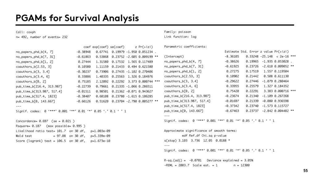
55. 55 Family: poisson Link function: log Parametric coefficients: Estimate Std. Error z value Pr(>|z|) (Intercept) -8.36105 0.33248 -25.148 < 2e-16 *** no_papers_phd_b(4, 7] -0.38626 0.19965 -1.935 0.053028 . no_papers_phd_b(7, 31] -0.61925 0.23726 -2.610 0.009052 ** no_papers_phd_b[1, 2] 0.27275 0.17519 1.557 0.119504 coauthors_b(2.53, 3] 0.10902 0.21442 0.508 0.611130 coauthors_b(3, 3.4] -0.29622 0.27446 -1.079 0.280464 coauthors_b(3.4, 6] 0.33955 0.25579 1.327 0.184352 coauthors_b[0, 2] 0.75420 0.22291 3.383 0.000716 *** pub_time_b(216.4, 313.987] -0.23674 0.21340 -1.109 0.267268 pub_time_b(313.987, 517.4] -0.01697 0.21339 -0.080 0.936598 pub_time_b(517.4, 1823] -0.37342 0.23740 -1.573 0.115727 pub_time_b[0, 143.667] -0.67463 0.23737 -2.842 0.004482 ** --- Signif. codes: 0 ‘***’ 0.001 ‘**’ 0.01 ‘*’ 0.05 ‘.’ 0.1 ‘ ’ 1 Approximate significance of smooth terms: edf Ref.df Chi.sq p-value s(stop) 3.103 3.736 12.05 0.0188 * --- Signif. codes: 0 ‘***’ 0.001 ‘**’ 0.01 ‘*’ 0.05 ‘.’ 0.1 ‘ ’ 1 R-sq.(adj) = -0.0701 Deviance explained = 3.05% -REML = 2003.7 Scale est. = 1 n = 12300 Call: coxph n= 492, number of events= 232 coef exp(coef) se(coef) z Pr(>|z|) no_papers_phd_b(4, 7] -0.38948 0.67741 0.19979 -1.950 0.051234 . no_papers_phd_b(7, 31] -0.61863 0.53868 0.23752 -2.605 0.009199 ** no_papers_phd_b[1, 2] 0.27444 1.31580 0.17532 1.565 0.117489 coauthors_b(2.53, 3] 0.10580 1.11159 0.21433 0.494 0.621580 coauthors_b(3, 3.4] -0.30237 0.73906 0.27435 -1.102 0.270406 coauthors_b(3.4, 6] 0.33886 1.40335 0.25563 1.326 0.184976 coauthors_b[0, 2] 0.75185 2.12092 0.22292 3.373 0.000744 *** pub_time_b(216.4, 313.987] -0.22739 0.79661 0.21335 -1.066 0.286511 pub_time_b(313.987, 517.4] -0.01511 0.98501 0.21362 -0.071 0.943627 pub_time_b(517.4, 1823] -0.38407 0.68108 0.23780 -1.615 0.106285 pub_time_b[0, 143.667] -0.66126 0.51620 0.23704 -2.790 0.005277 ** --- Signif. codes: 0 ‘***’ 0.001 ‘**’ 0.01 ‘*’ 0.05 ‘.’ 0.1 ‘ ’ 1 Concordance= 0.697 (se = 0.021 ) Rsquare= 0.187 (max possible= 0.995 ) Likelihood ratio test= 101.7 on 30 df, p=1.003e-09 Wald test = 97.08 on 30 df, p=5.339e-09 Score (logrank) test = 106.5 on 30 df, p=1.673e-10 PGAMs for Survival Analysis
56. 56 Random Forests These are generalisations of Random Forests for duration data. In Random Forests, randomisation is introduced by randomly drawing a bootstrapped sample of data to grow the tree and then growing it by splitting nodes on randomly selected predictors. Bonus points: • Only three parameters to set; number of randomly selected predictors, number of trees to grow and splitting rule. • No assumptions. Unnecessary to demand proportional hazards, etc. Random Survival Forests are implemented through the library randomForestSRC. Training a forest yields an ensemble estimate for the cumulative hazard function Random Survival Forests http://bit.ly/1SSWYd7
57. 57 Random Forests Random Survival Forests library('randomForestSRC') library('ggRandomForests') ntree <- 1000 my_features <- c('delta', 'observed','phd_place' , 'no_papers_phd_b', 'coauthors_b', ‘pub_time_b’, ‘independence_flag’) rfsrc_pbc <- rfsrc( Surv(delta, observed) ~ ., data = train[, my_features], nsplit = 10, na.action = "na.impute") ggRFsrc <- plot( gg_rfsrc(rfsrc_pbc), alpha = 0.2 ) + labs(y = "Survival Probability", x = "Time (days)") + coord_cartesian(ylim = c(-0.01, 1.01)) + theme_minimal() + theme(legend.position = ‘bottom') show(ggRFsrc) Very simple to train if you have worked with Random Forests for Classification or Regression tasks before:
58. 58 Random Survival Forests Training Set Test Set
59. 59 Random Survival Forests We also get variable importance as a freebie:
60. 60 TL;DR
61. Surviving Academia 9 years is the median academic lifetime By year 9, for an individual there is a 50% he/she will still be in academia; this is roughly equivalent to a PhD and 1-2 postdocs. Lots of papers during PhD are a good indicator of survival Publish or die! Be a good networker Many collaborations = many papers + opportunities Choosing the right place for a PhD helps Facilitate creation of networks (?) 61 Data consistent with trends of women in STEM
62. Survival Analysis Extremely useful technique Applicable to many problems in various fields Good Python Library with estimators & regressors Thanks Cam Davidson-Pilon! More stuff available in R Above + GAMs, Random Survival Forests Other approaches - Bayesian Tutorial on the subject yesterday! 62
63. 63 Thanks!