R project

Transcript

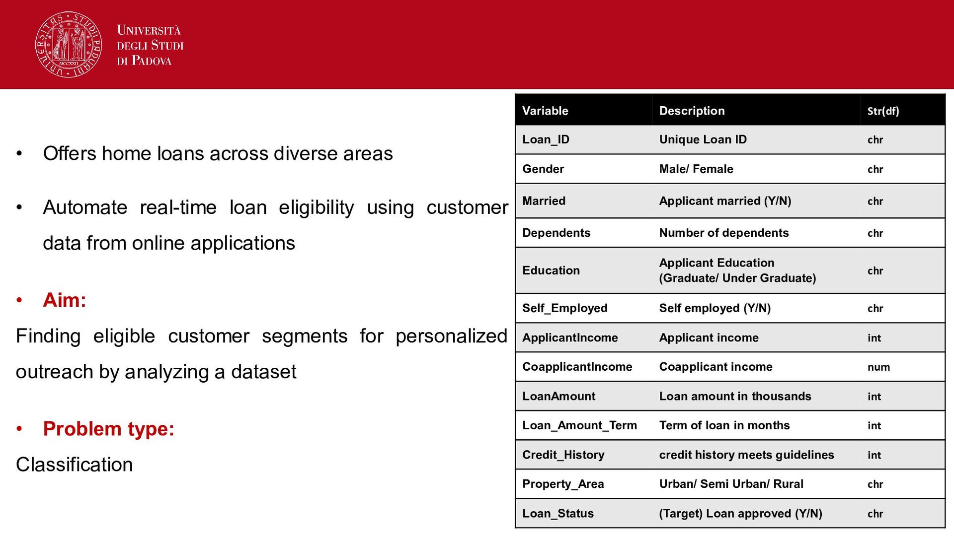
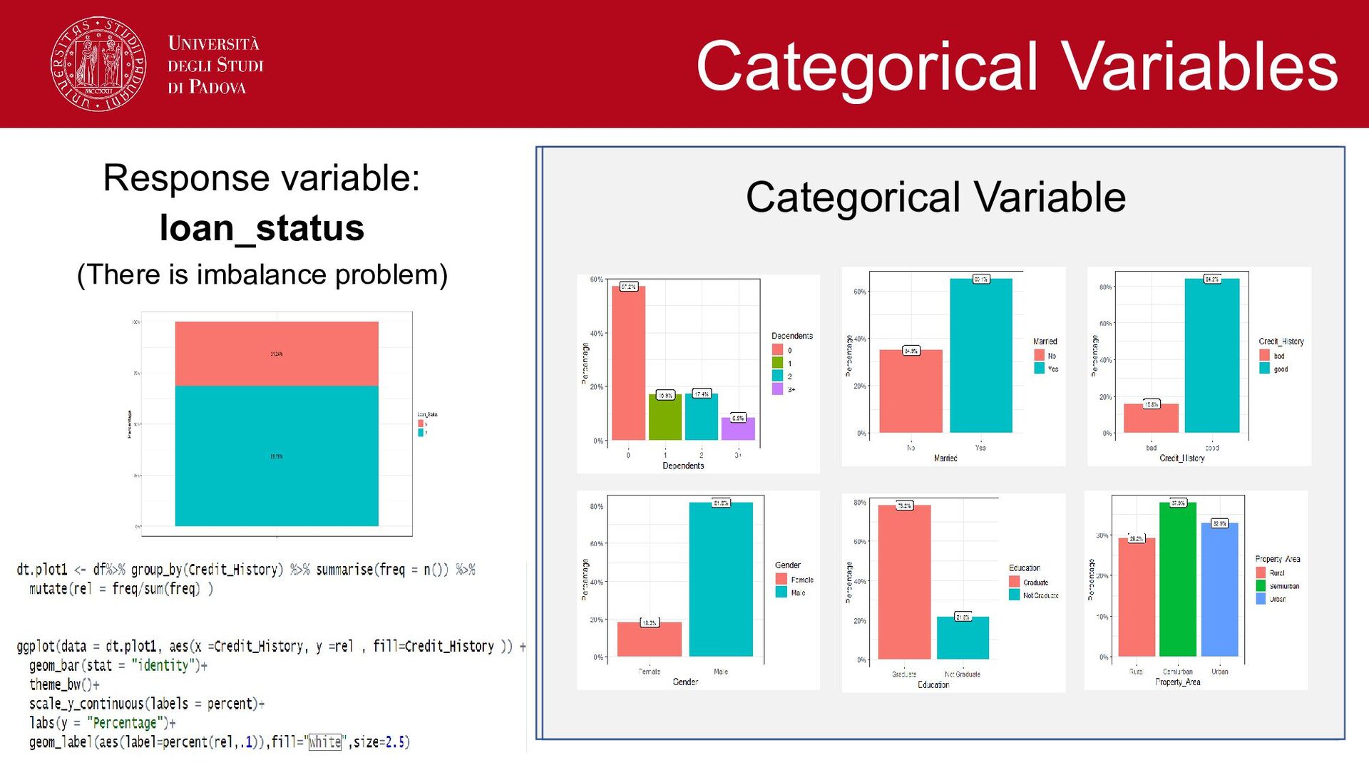
1. • Offers home loans across diverse areas • Automate real-time loan eligibility using customer data from online applications • Aim: Finding eligible customer segments for personalized outreach by analyzing a dataset • Problem type: Classification Variable Description Str(df) Loan_ID Unique Loan ID chr Gender Male/ Female chr Married Applicant married (Y/N) chr Dependents Number of dependents chr Education Applicant Education (Graduate/ Under Graduate) chr Self_Employed Self employed (Y/N) chr ApplicantIncome Applicant income int CoapplicantIncome Coapplicant income num LoanAmount Loan amount in thousands int Loan_Amount_Term Term of loan in months int Credit_History credit history meets guidelines int Property_Area Urban/ Semi Urban/ Rural chr Loan_Status (Target) Loan approved (Y/N) chr
2. • ID variable has omitted • Assign missing values as NA • Characters were converted to factors (Credit history has converted to good and bad factors) Data Preparation
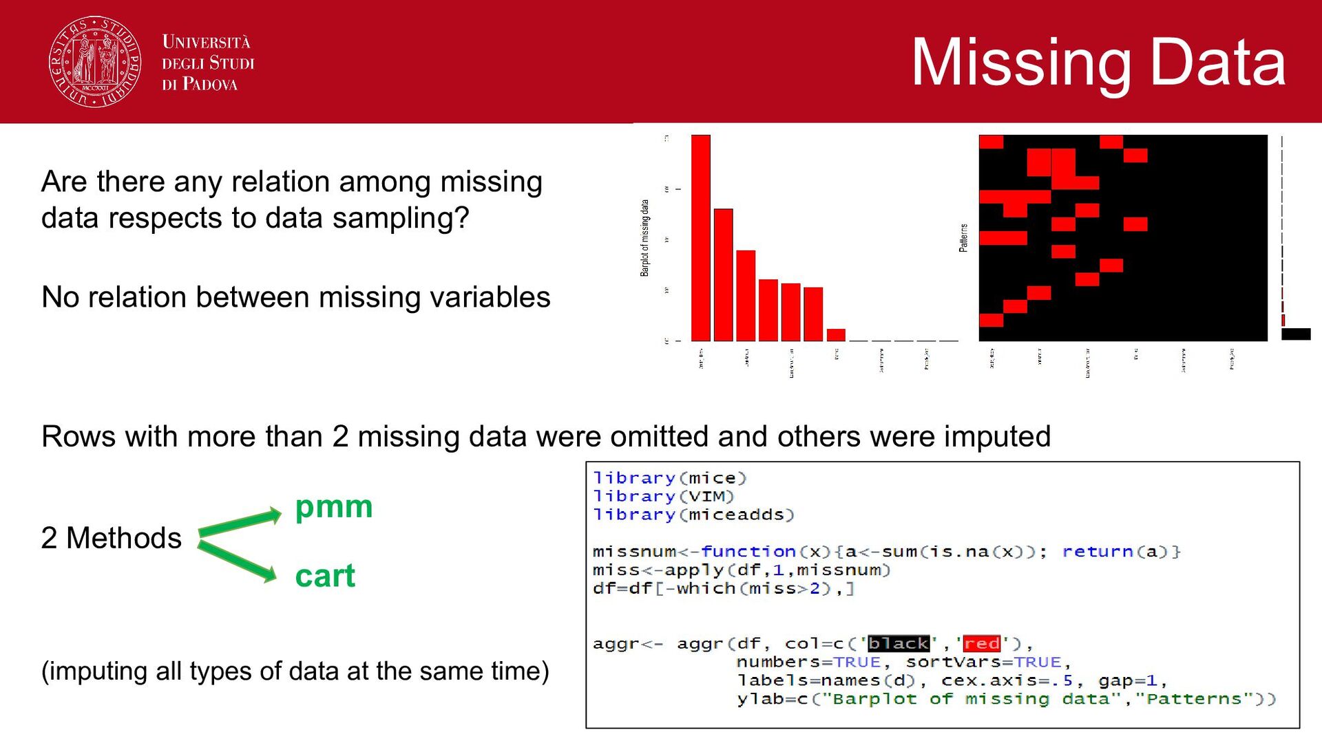
3. Are there any relation among missing data respects to data sampling? No relation between missing variables Rows with more than 2 missing data were omitted and others were imputed 2 Methods (imputing all types of data at the same time) Missing Data pmm cart
4. Imputation Cart has been chosen because it mimics the original distribution better Distribution of “LoanAmount” before (red) and after (green , blue) imputation
5. Categorical Variable Response variable: loan_status (There is imbalance problem) Categorical Variables
6. Bayesian method used to find which categorical variables has influence on the response Bayesian Method
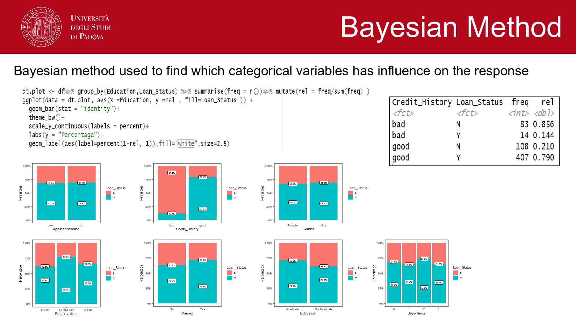
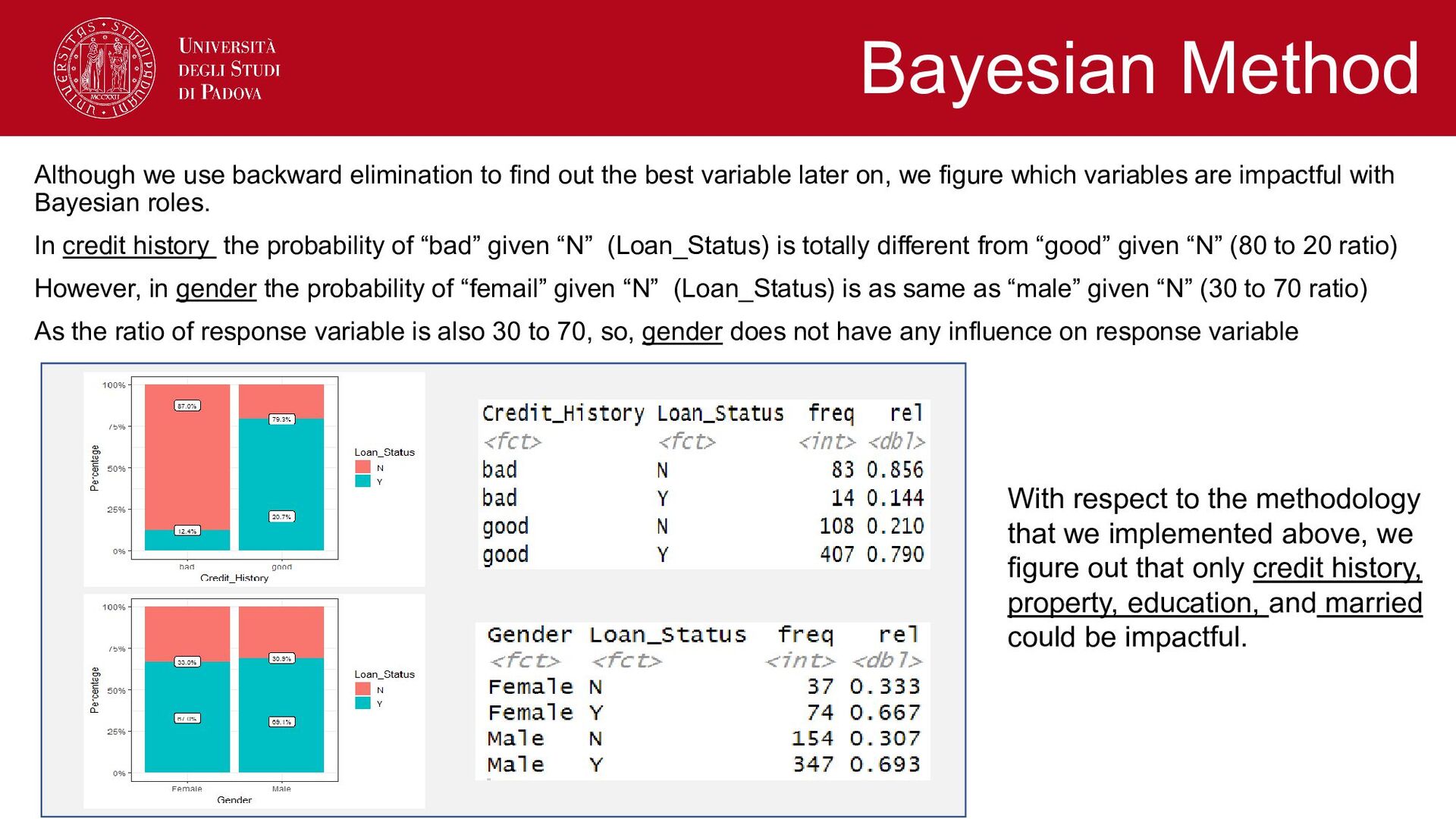
7. Although we use backward elimination to find out the best variable later on, we figure which variables are impactful with Bayesian roles. In credit history the probability of “bad” given “N” (Loan_Status) is totally different from “good” given “N” (80 to 20 ratio) However, in gender the probability of “femail” given “N” (Loan_Status) is as same as “male” given “N” (30 to 70 ratio) As the ratio of response variable is also 30 to 70, so, gender does not have any influence on response variable Bayesian Method With respect to the methodology that we implemented above, we figure out that only credit history, property, education, and married could be impactful.
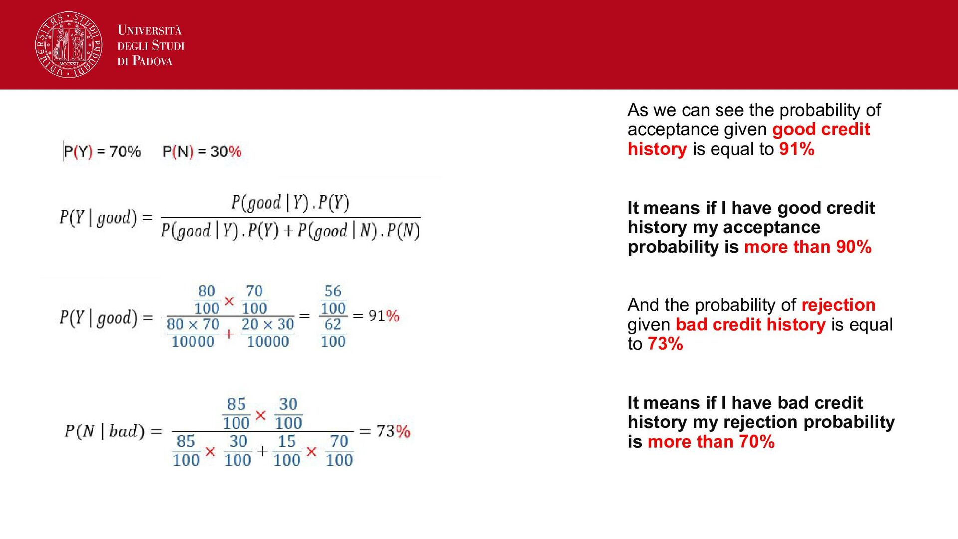
8. As we can see the probability of acceptance given good credit history is equal to 91% It means if I have good credit history my acceptance probability is more than 90% And the probability of rejection given bad credit history is equal to 73% It means if I have bad credit history my rejection probability is more than 70%
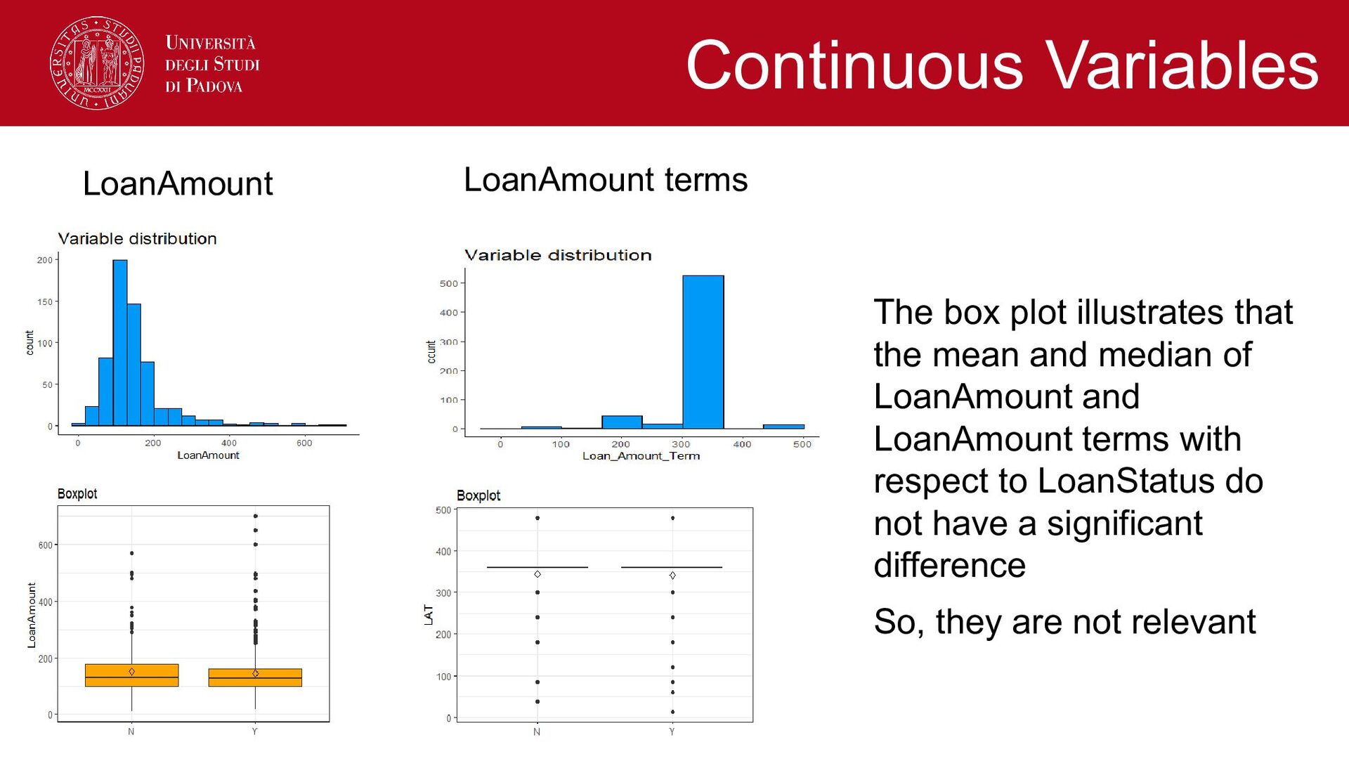
9. LoanAmount LoanAmount terms The box plot illustrates that the mean and median of LoanAmount and LoanAmount terms with respect to LoanStatus do not have a significant difference So, they are not relevant Continuous Variables
10. 75-25 train- test split Splitting data
11. Classification analysis Trained Logistic Regression Model
12. N Y N 27 6 Y 20 99
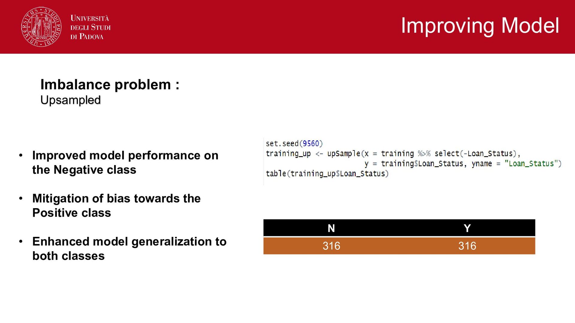
13. Imbalance problem : Upsampled N Y 316 316 • Improved model performance on the Negative class • Mitigation of bias towards the Positive class • Enhanced model generalization to both classes Improving Model
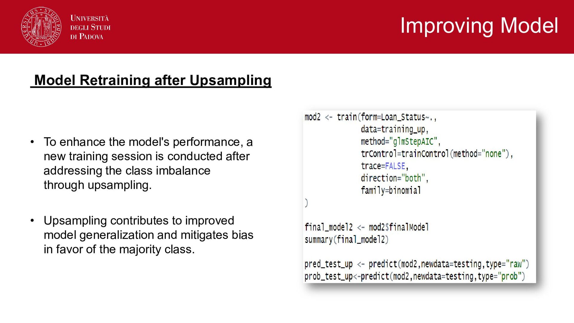
14. Model Retraining after Upsampling • To enhance the model's performance, a new training session is conducted after addressing the class imbalance through upsampling. • Upsampling contributes to improved model generalization and mitigates bias in favor of the majority class. Improving Model
15. N Y N 32 29 Y 15 85
16. Exploring Threshold Sensitivity in Logistic Regression : 0.4 0.6 Threshold Sensitivity
17. Part 2
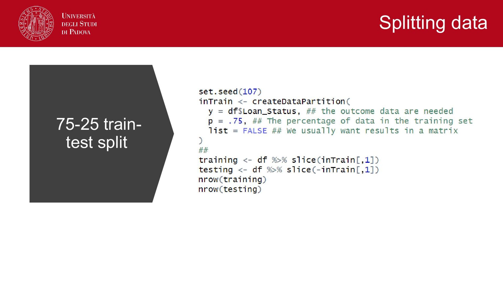
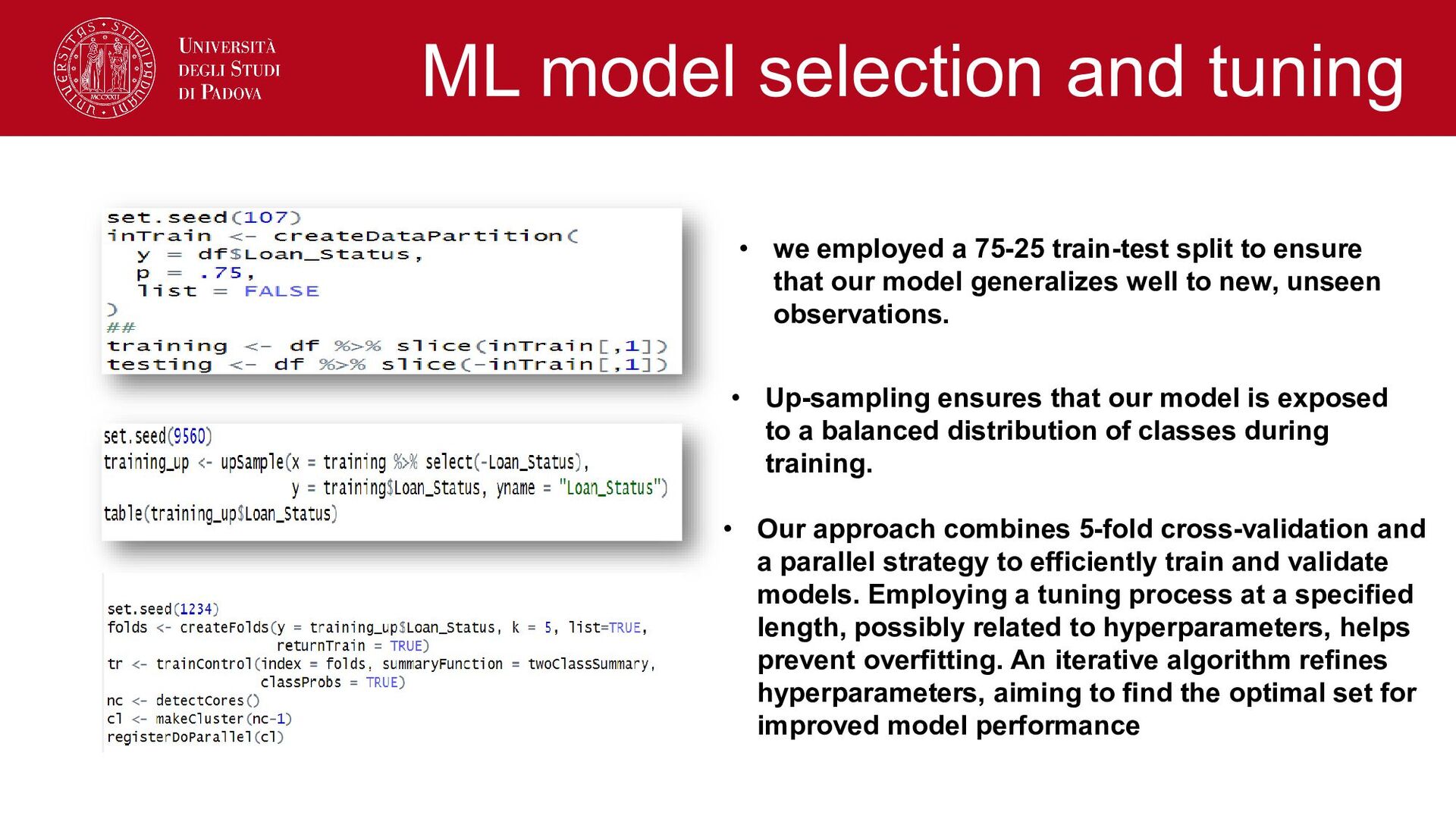
18. ML model selection and tuning • Up-sampling ensures that our model is exposed to a balanced distribution of classes during training. • we employed a 75-25 train-test split to ensure that our model generalizes well to new, unseen observations. • Our approach combines 5-fold cross-validation and a parallel strategy to efficiently train and validate models. Employing a tuning process at a specified length, possibly related to hyperparameters, helps prevent overfitting. An iterative algorithm refines hyperparameters, aiming to find the optimal set for improved model performance
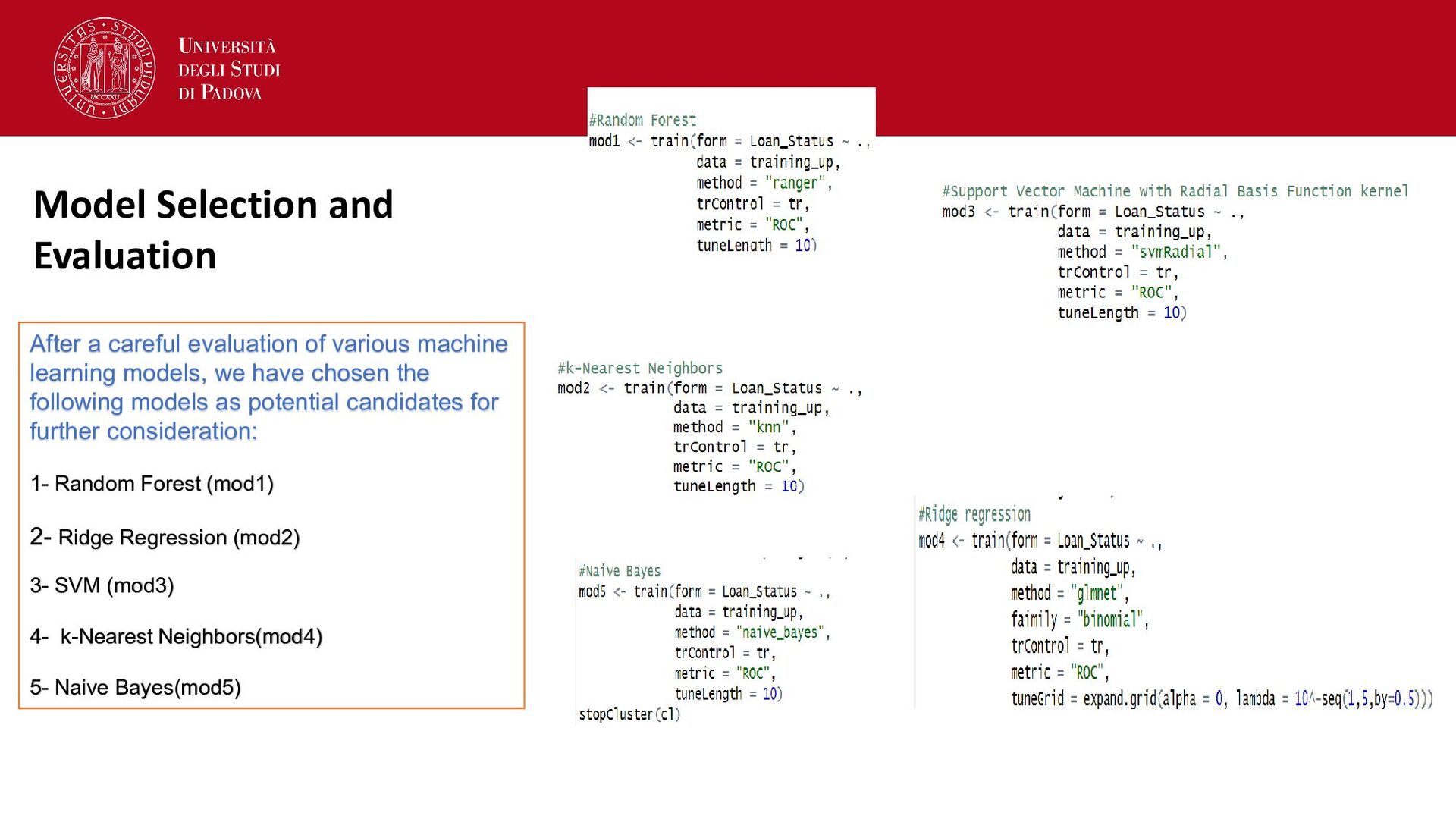
19. Model Selection and Evaluation After a careful evaluation of various machine learning models, we have chosen the following models as potential candidates for further consideration: 1- Random Forest (mod1) 2- Ridge Regression (mod2) 3- SVM (mod3) 4- k-Nearest Neighbors(mod4) 5- Naive Bayes(mod5)
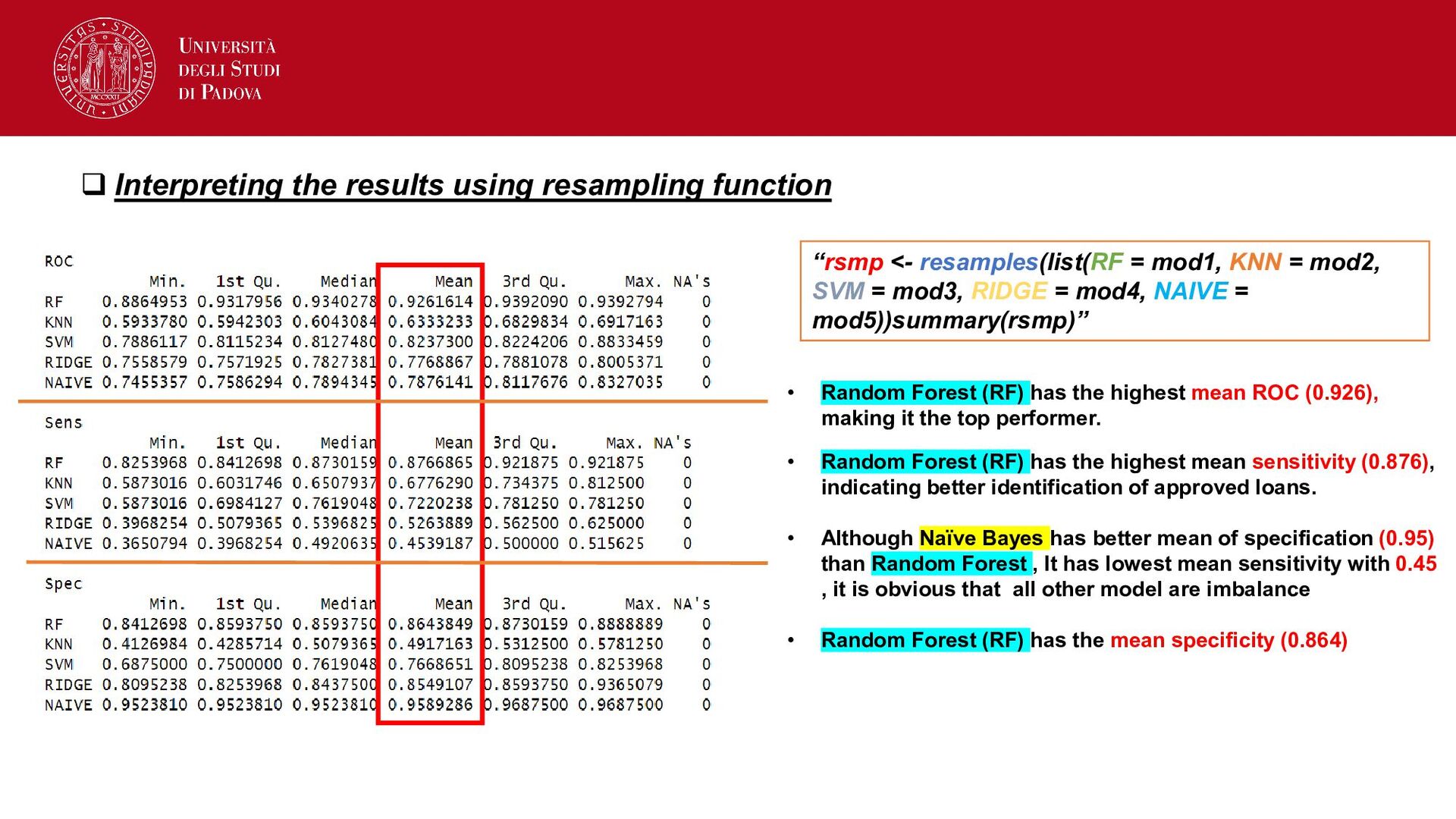
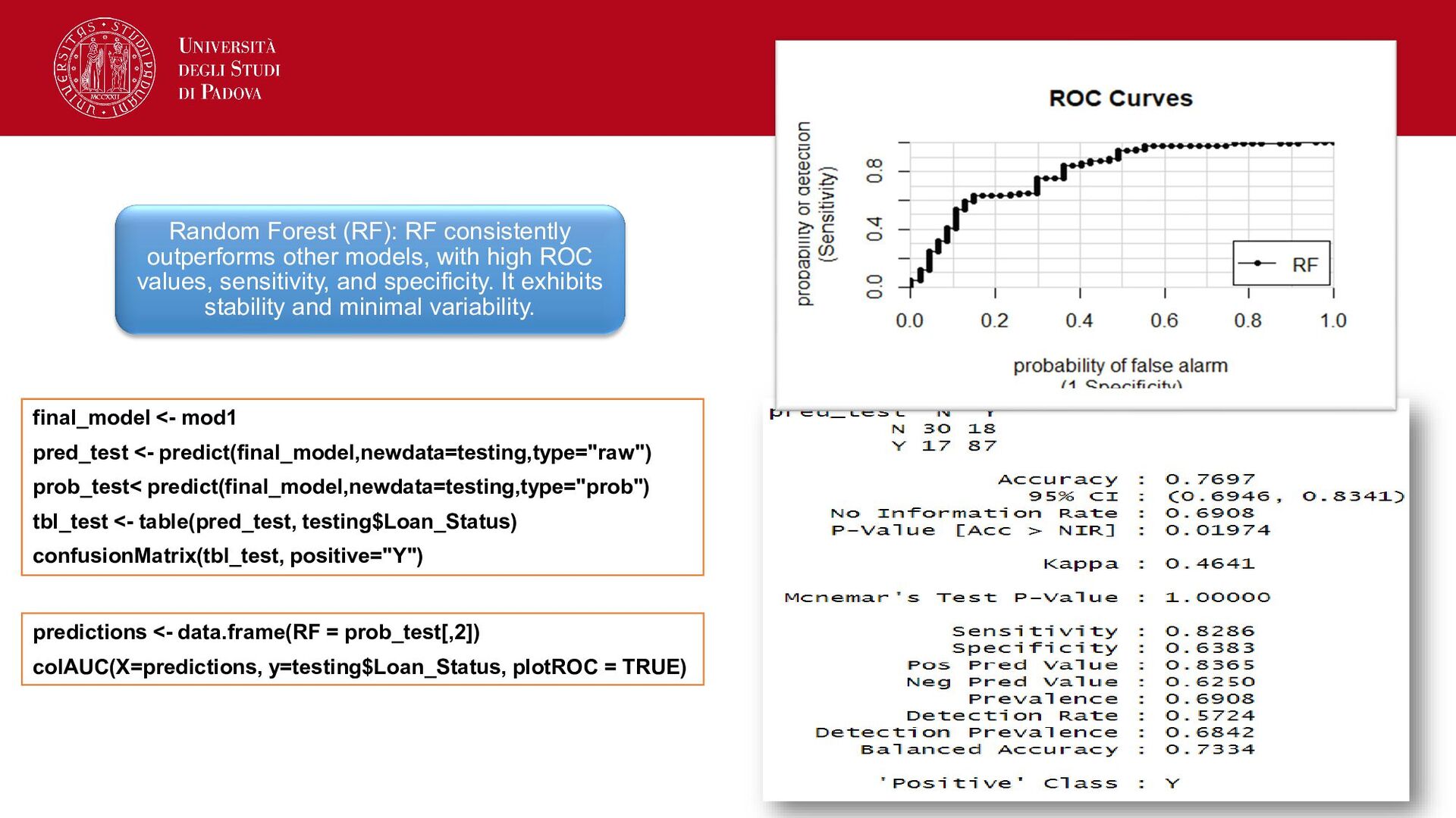
20.  Interpreting the results using resampling function • Random Forest (RF) has the highest mean ROC (0.926), making it the top performer. • Random Forest (RF) has the highest mean sensitivity (0.876), indicating better identification of approved loans. • Although Naïve Bayes has better mean of specification (0.95) than Random Forest , It has lowest mean sensitivity with 0.45 , it is obvious that all other model are imbalance • Random Forest (RF) has the mean specificity (0.864) “rsmp <- resamples(list(RF = mod1, KNN = mod2, SVM = mod3, RIDGE = mod4, NAIVE = mod5))summary(rsmp)”
21. Further Comparing Performances bwplot(rsmp, layout = c(3, 1), scales = "free") dotplot(rsmp, metric = "ROC") Box Plots (bwplot) Dot Plot (dotplot)
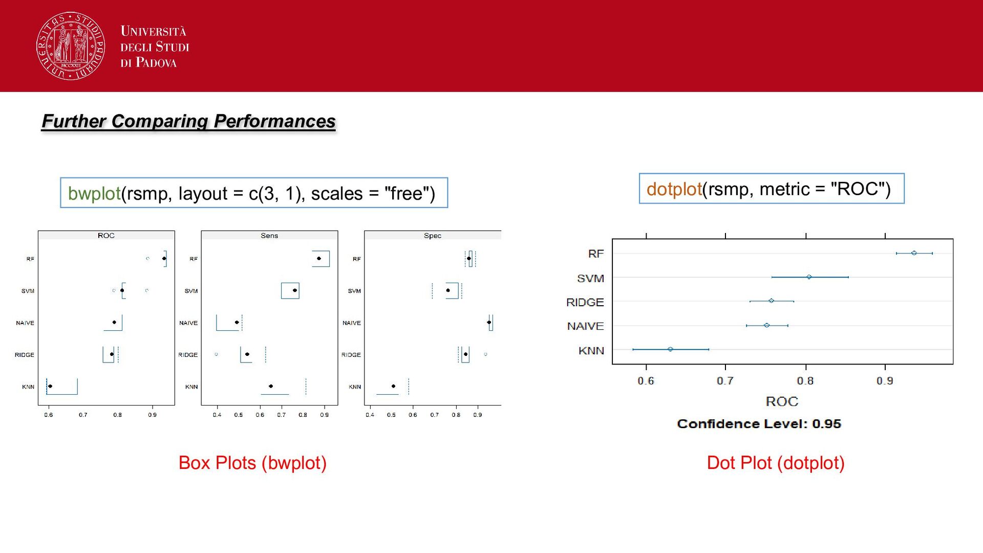
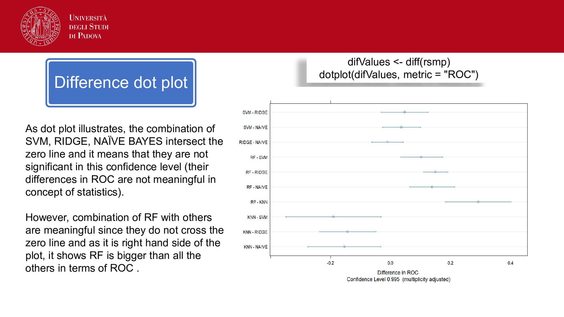
22. Difference dot plot difValues <- diff(rsmp) dotplot(difValues, metric = "ROC") As dot plot illustrates, the combination of SVM, RIDGE, NAÏVE BAYES intersect the zero line and it means that they are not significant in this confidence level (their differences in ROC are not meaningful in concept of statistics). However, combination of RF with others are meaningful since they do not cross the zero line and as it is right hand side of the plot, it shows RF is bigger than all the others in terms of ROC .
23. Random Forest (RF): RF consistently outperforms other models, with high ROC values, sensitivity, and specificity. It exhibits stability and minimal variability. final_model <- mod1 pred_test <- predict(final_model,newdata=testing,type="raw") prob_test< predict(final_model,newdata=testing,type="prob") tbl_test <- table(pred_test, testing$Loan_Status) confusionMatrix(tbl_test, positive="Y") predictions <- data.frame(RF = prob_test[,2]) colAUC(X=predictions, y=testing$Loan_Status, plotROC = TRUE)
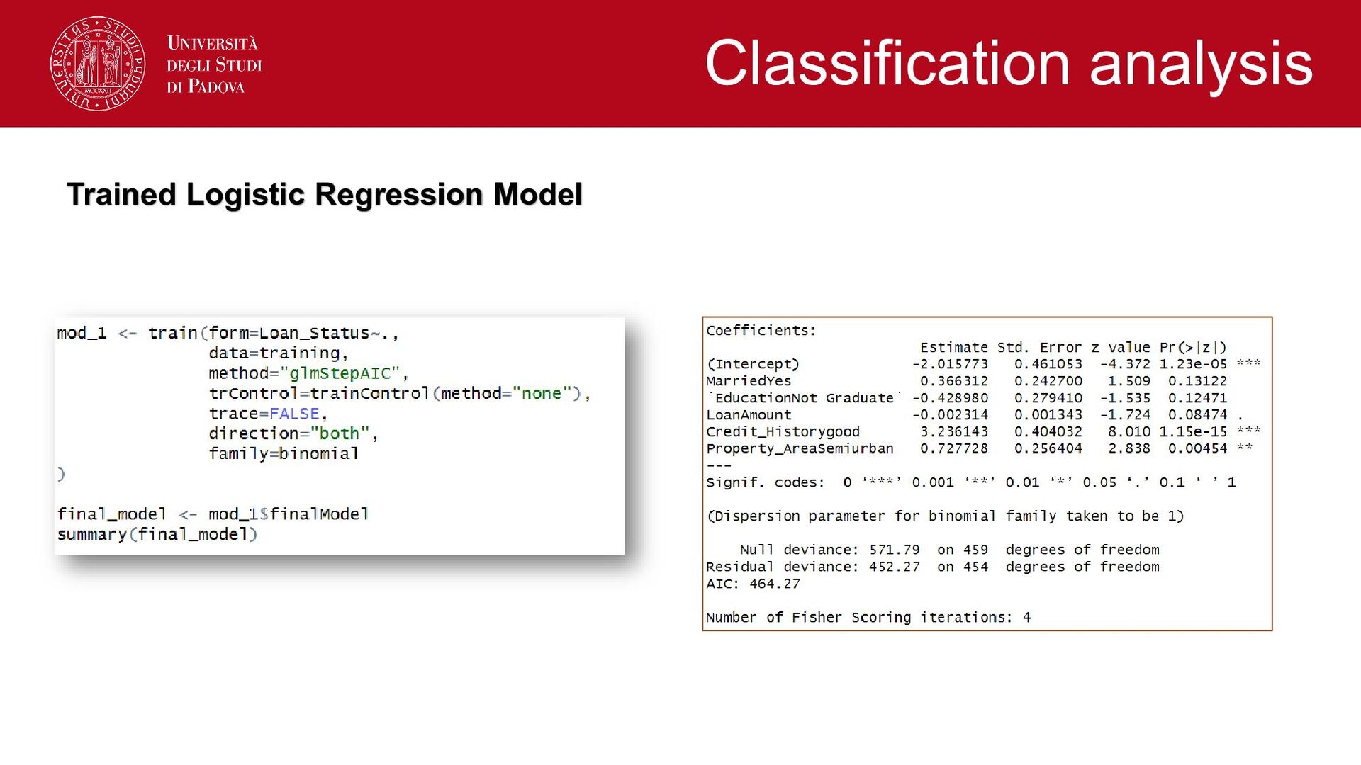
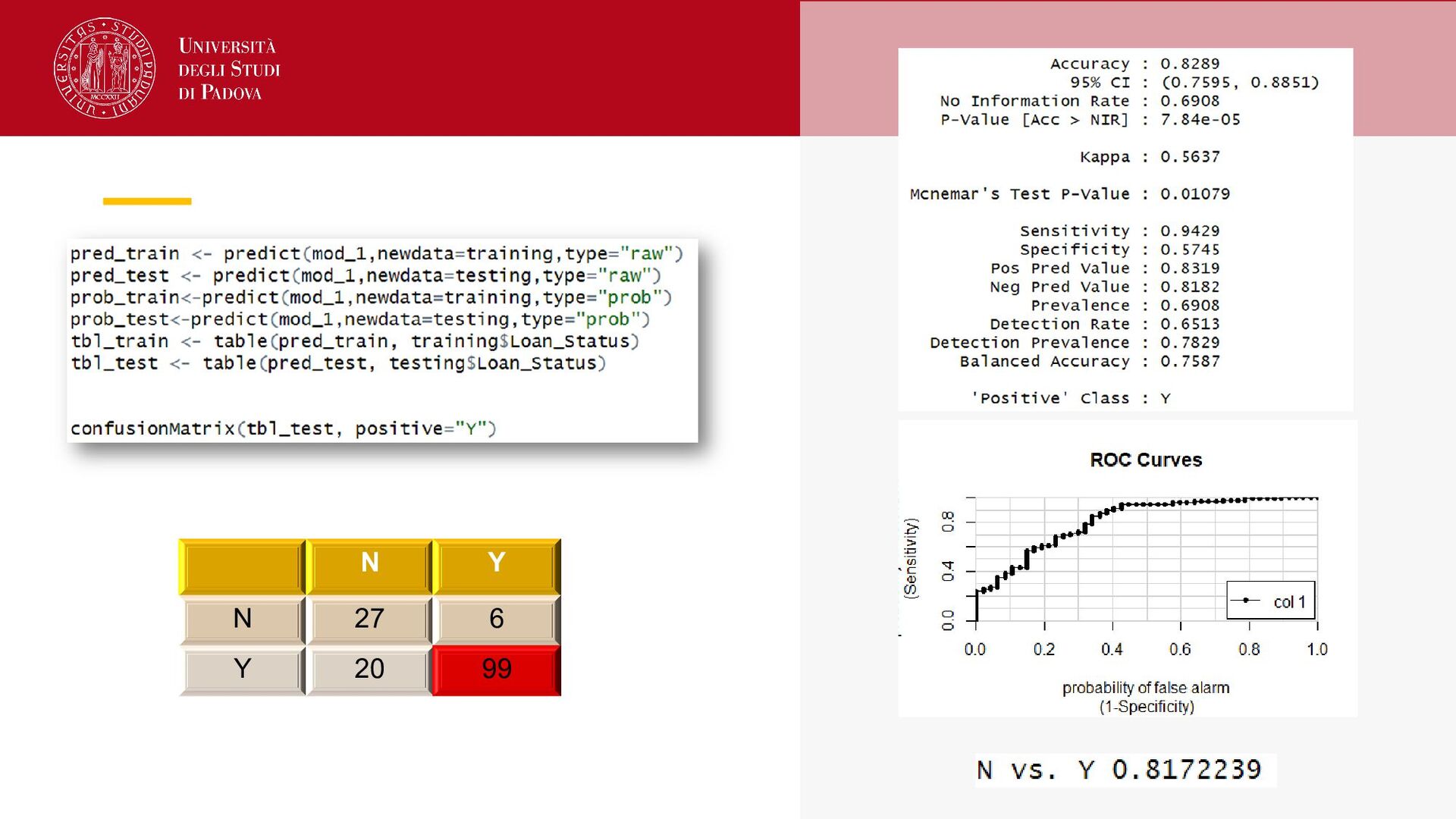
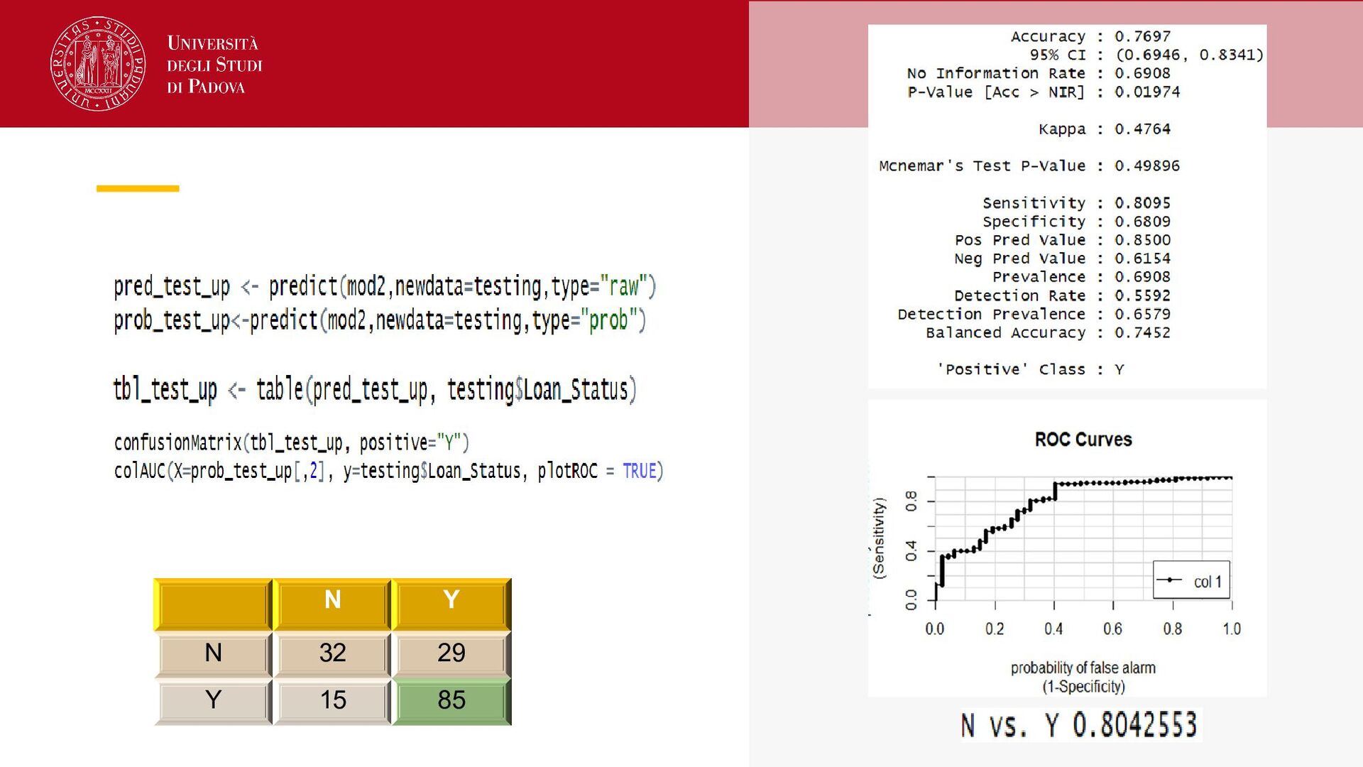
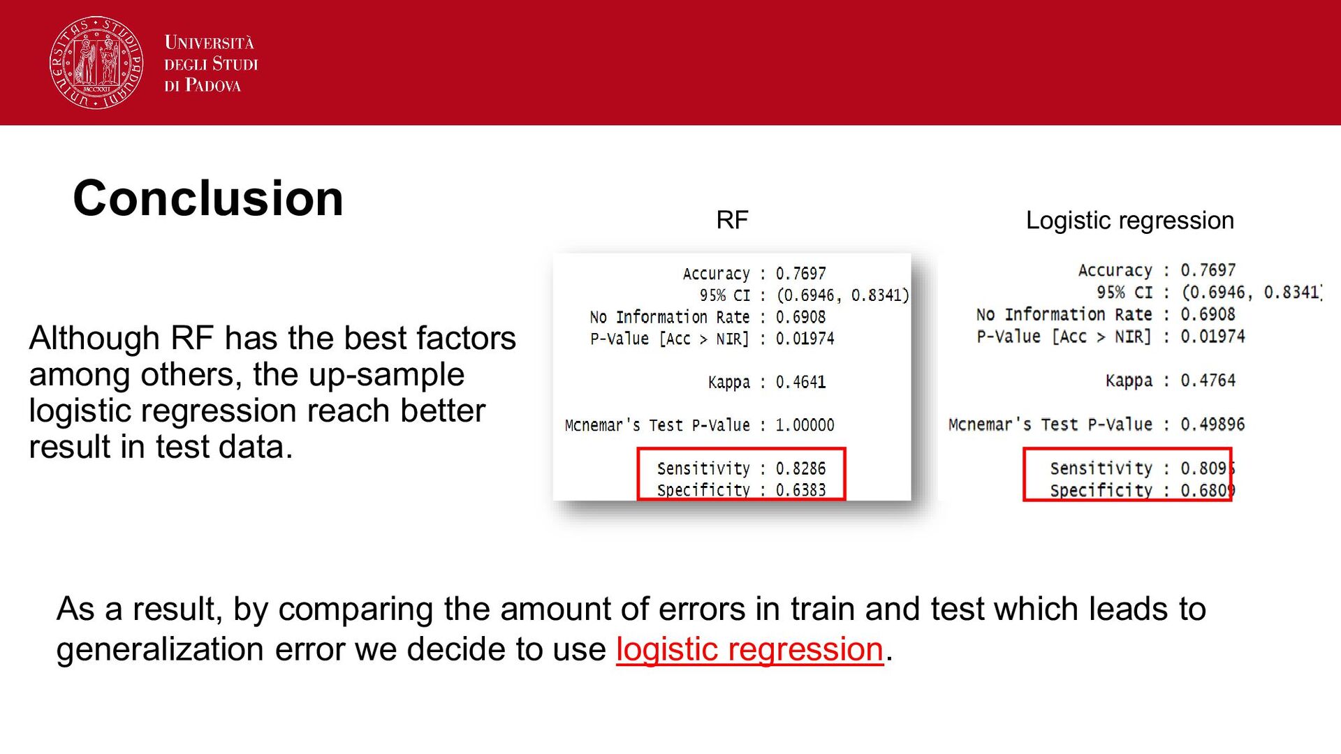
24. Conclusion Although RF has the best factors among others, the up-sample logistic regression reach better result in test data. RF Logistic regression As a result, by comparing the amount of errors in train and test which leads to generalization error we decide to use logistic regression.