Scientist. • Worked in Bing data mining, Bing Ads (2006-2013) • ETL, bot detection, online experimentation and A/B testing, relevance of online ads, click prediction, etc. • Ph.D. in CS with a focus on computer vision, machine learning and data mining. Copyright (c) 2018. Data Science Dojo 2
• Worked in game engine technology, writing technical content on new features. • Graduate diploma in mathematics and statistics, with a bachelor degree in information and media. Copyright (c) 2018. Data Science Dojo 3
Worked for a small research consultancy in London and worked on projects for governments, international organizations and companies such as the UN and Siemens. • BA in Human Sciences from Oxford University and an MSc in Decision Science. Copyright (c) 2018. Data Science Dojo 4
scientist at McKinsey & Company, Sydney • Bachelor’s in Computer Science and Mathematics from Télécom Paristech (“Grande Ecole”), and a Master’s in Statistics from Imperial College, London. Copyright (c) 2018. Data Science Dojo 5
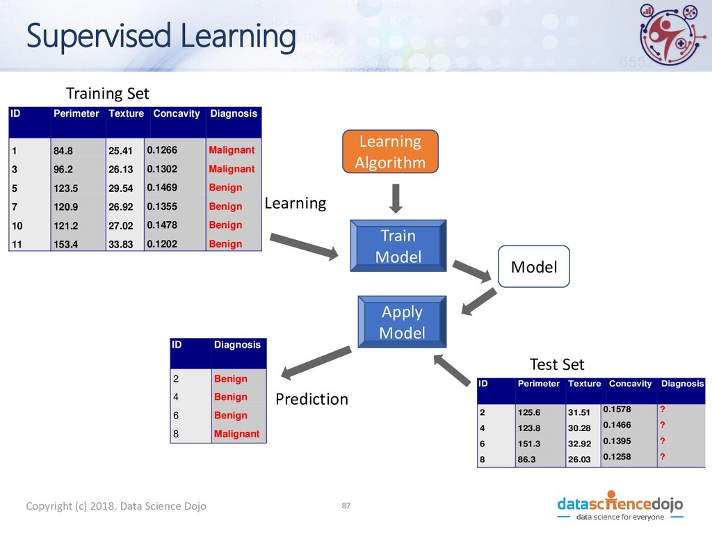
science for improved health systems and healthcare. • Explore and visualize a health-related dataset. • Build and evaluate predictive models for classification and regression (for instance, predicting whether a tumour is malignant or not), as an example of the use of machine learning in health. Copyright (c) 2018. Data Science Dojo 7
clustering, and its potential applications in health systems • Learn fundamentals of text analytics and perform text analytics on a health-related dataset • Get an introduction to big data and data engineering Copyright (c) 2018. Data Science Dojo 8
problems at all times: •Problem and business impact •Data you have (and do not have). •Measurement metrics •Business metrics 10 Copyright (c) 2018. Data Science Dojo
material and resources: • Handbooks • Learning portal • Request: • Make sure your computers are ready • Keep the session interactive • Social media, email, etc. Copyright (c) 2018. Data Science Dojo 11 *We will end at 4:00 pm on Friday
science landscape Session II: Data exploration and visualization Session III: Introduction to predictive modeling Session IV: Decision tree learning and building your first predictive model Session V: Evaluating classification models Copyright (c) 2018. Data Science Dojo 12
what other organizations are (or may be) doing • Common data mining tasks • Identify some data science problems in health Copyright (c) 2018. Data Science Dojo 14
treatments including immunotherapies. • MIT Clinical Machine Learning Group • Focussed on disease processes and design for effective treatment of diseases such as Type 2 diabetes. • Knight Cancer Institute • With a current focus on developing an approach to personalize drug combinations for Acute Myeloid Leukemia (AML). Copyright (c) 2018. Data Science Dojo 15
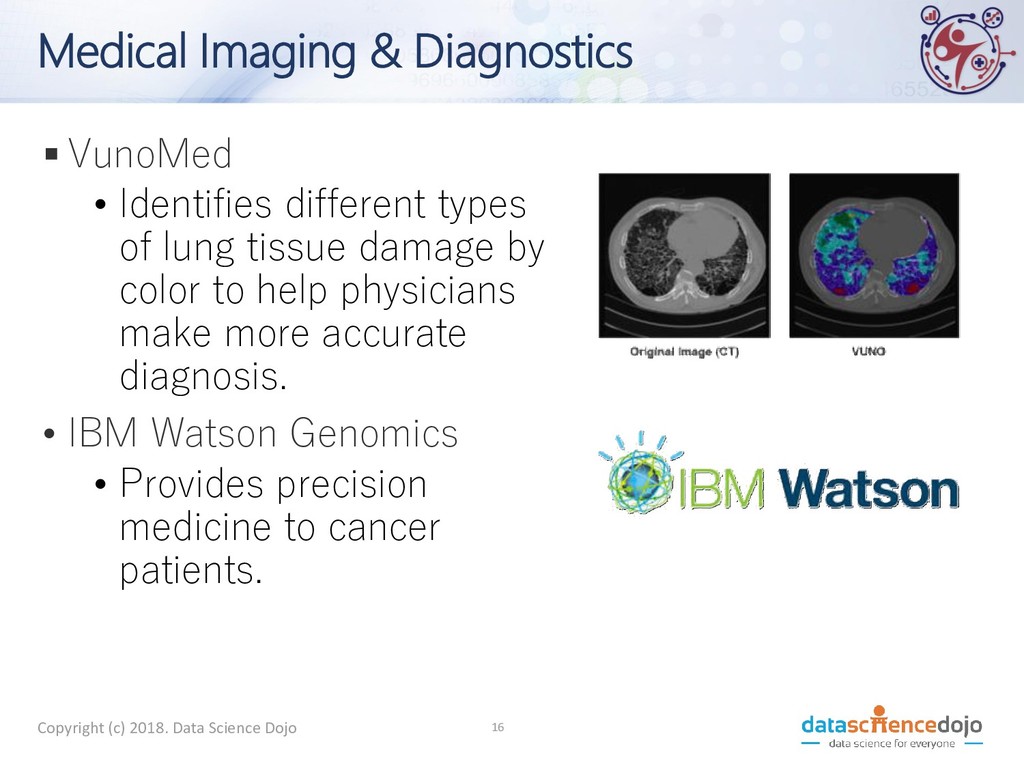
of lung tissue damage by color to help physicians make more accurate diagnosis. • IBM Watson Genomics • Provides precision medicine to cancer patients. Copyright (c) 2018. Data Science Dojo 16
patients to get their lab results explained to them by an app, saving both patient and doctor time and money. • Somatix • Recognizes of hand-to-mouth gestures in order to help people better understand their behavior and make life-affirming changes. Copyright (c) 2018. Data Science Dojo 17
macular degeneration in aging eyes. • Desktop Genetics • AI-designed tech for more effective and affordable guides. Recognized as leader in genome editing technology. • iCarbonX • Monitors and models human biological data to enable people to find the proper lifestyle and treatments that can improve their health, life quality and joy. Copyright (c) 2018. Data Science Dojo 18
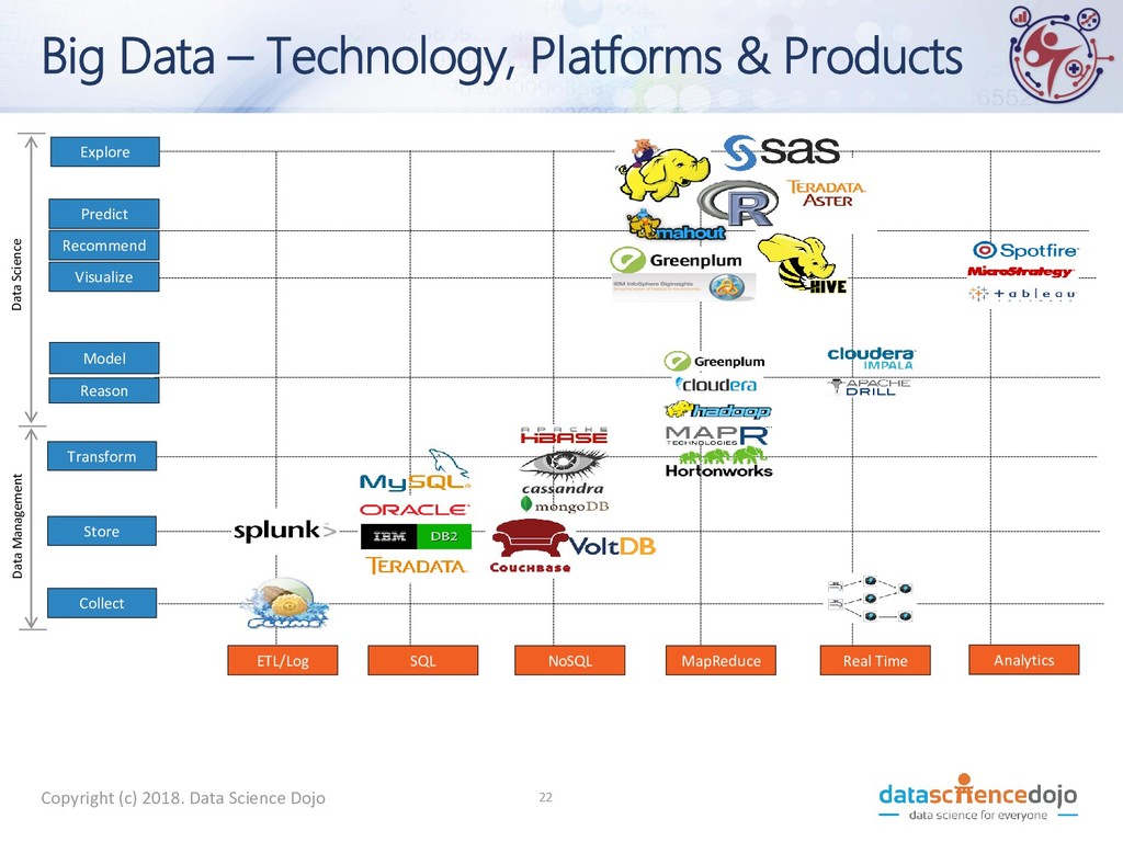
Recommend Predict Explore ETL/Log SQL NoSQL MapReduce Real Time Analytics Big Data – Technology, Platforms & Products Copyright (c) 2018. Data Science Dojo 22
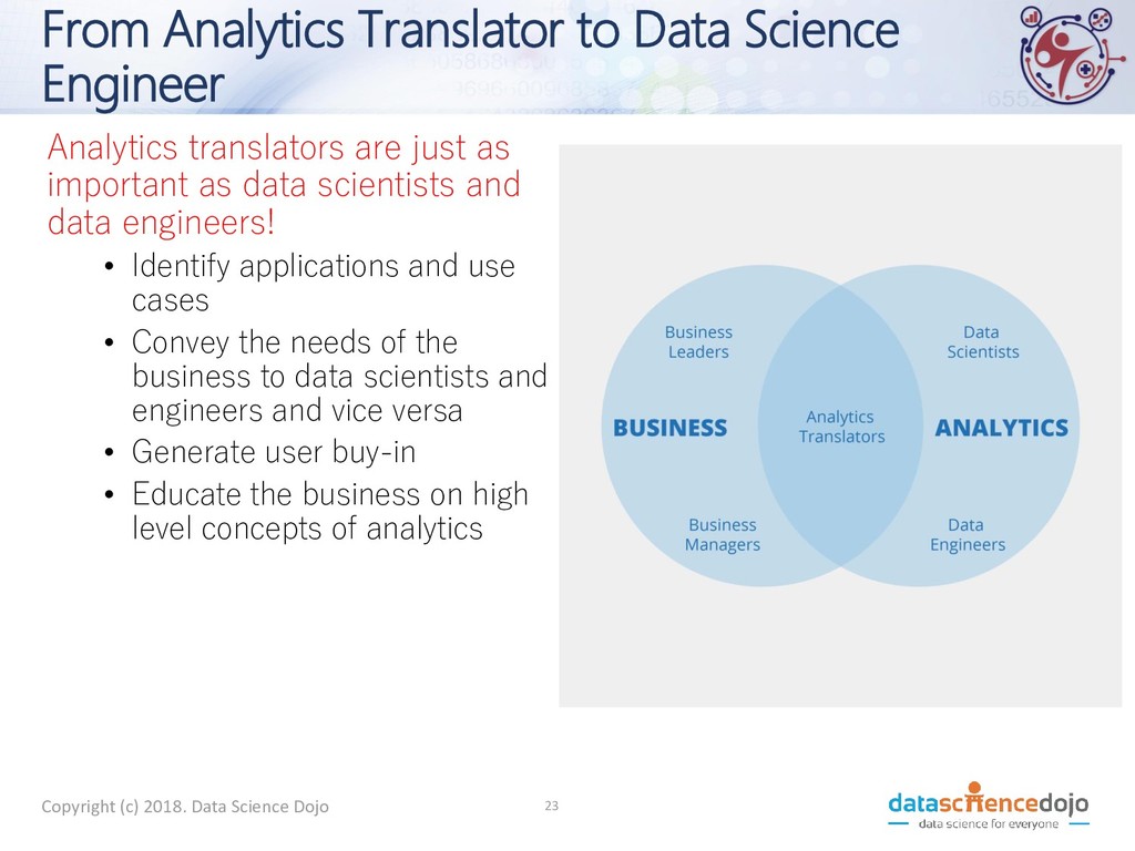
just as important as data scientists and data engineers! • Identify applications and use cases • Convey the needs of the business to data scientists and engineers and vice versa • Generate user buy-in • Educate the business on high level concepts of analytics 23 Copyright (c) 2018. Data Science Dojo
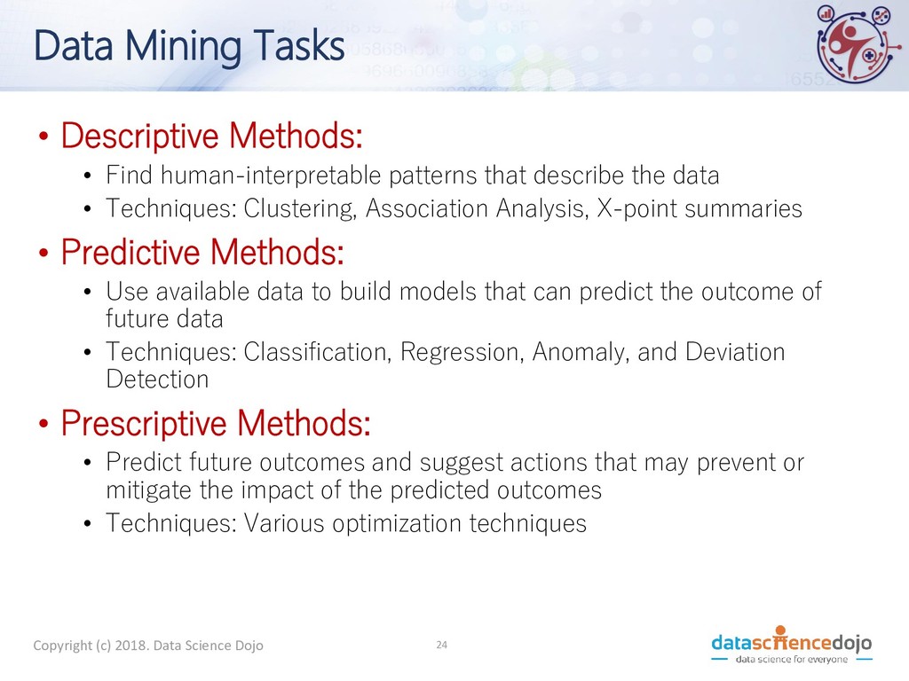
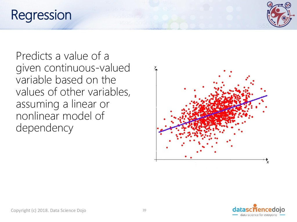
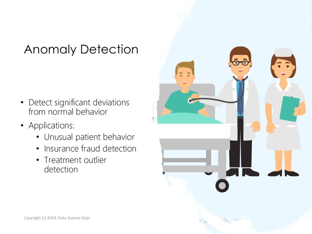
that describe the data • Techniques: Clustering, Association Analysis, X-point summaries • Predictive Methods: • Use available data to build models that can predict the outcome of future data • Techniques: Classification, Regression, Anomaly, and Deviation Detection • Prescriptive Methods: • Predict future outcomes and suggest actions that may prevent or mitigate the impact of the predicted outcomes • Techniques: Various optimization techniques Copyright (c) 2018. Data Science Dojo 24
so traffic jam does not happen OR Traffic jam is about to happen in the next 30 minutes and you could possibly take the following courses of action: • Route traffic to service road near I-5 • Block more traffic from entering the WA-520 bridge Copyright (c) 2018. Data Science Dojo 27
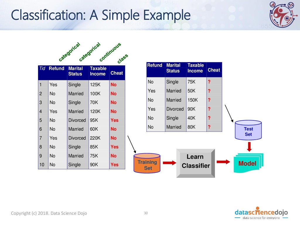
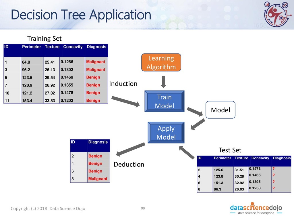
Cheat 1 Yes Single 125K No 2 No Married 100K No 3 No Single 70K No 4 Yes Married 120K No 5 No Divorced 95K Yes 6 No Married 60K No 7 Yes Divorced 220K No 8 No Single 85K Yes 9 No Married 75K No 10 No Single 90K Yes 10 Refund Marital Status Taxable Income Cheat No Single 75K ? Yes Married 50K ? No Married 150K ? Yes Divorced 90K ? No Single 40K ? No Married 80K ? 10 Test Set Training Set Model Learn Classifier Copyright (c) 2018. Data Science Dojo 30
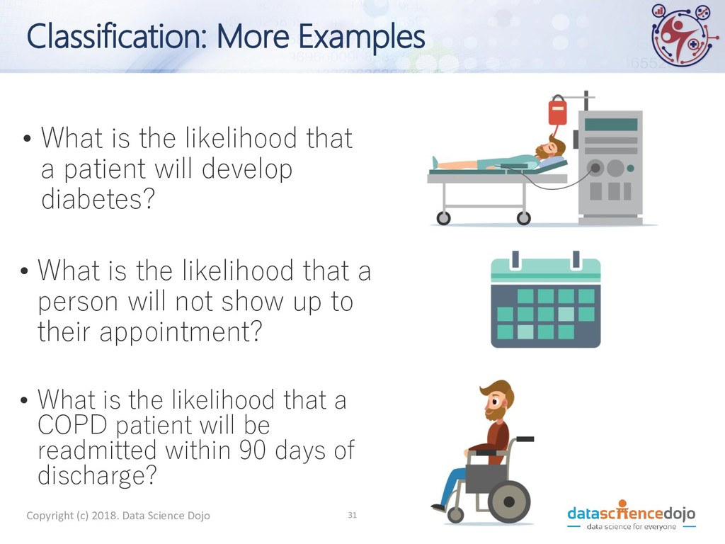
patient will develop diabetes? • What is the likelihood that a COPD patient will be readmitted within 90 days of discharge? • What is the likelihood that a person will not show up to their appointment? Copyright (c) 2018. Data Science Dojo 31
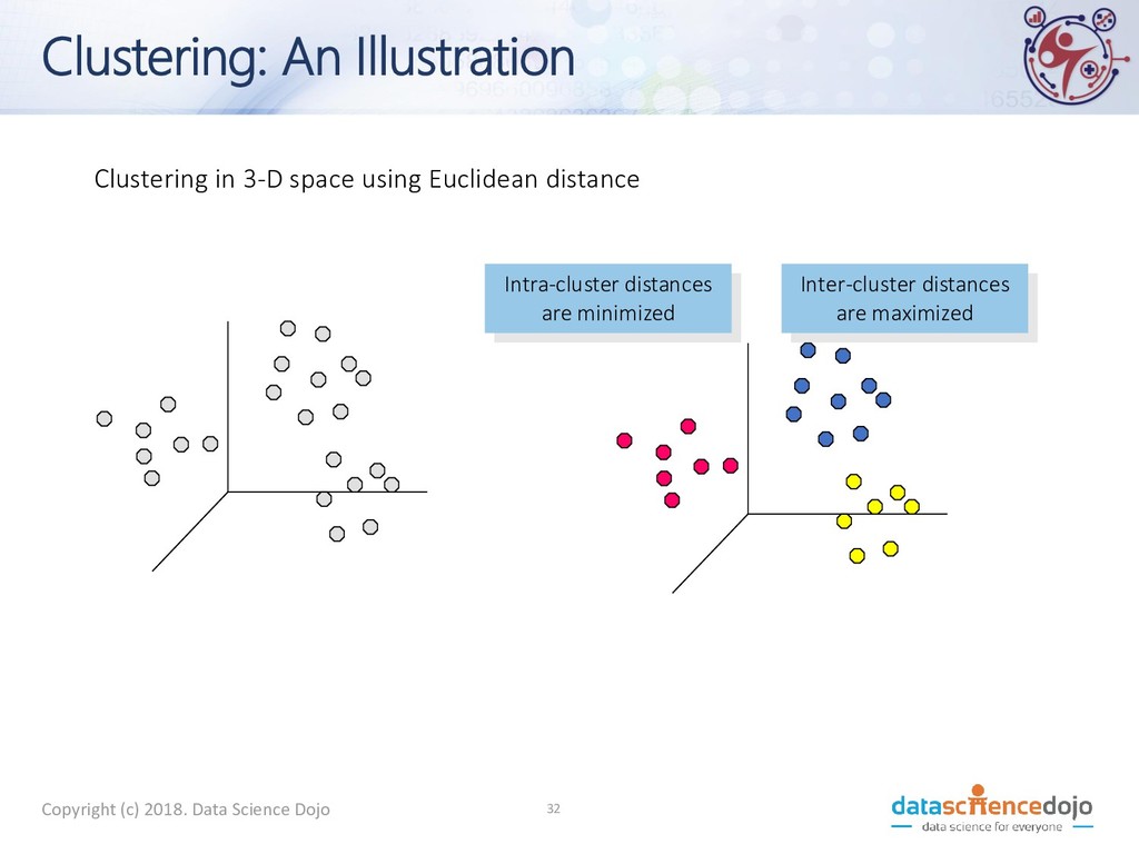
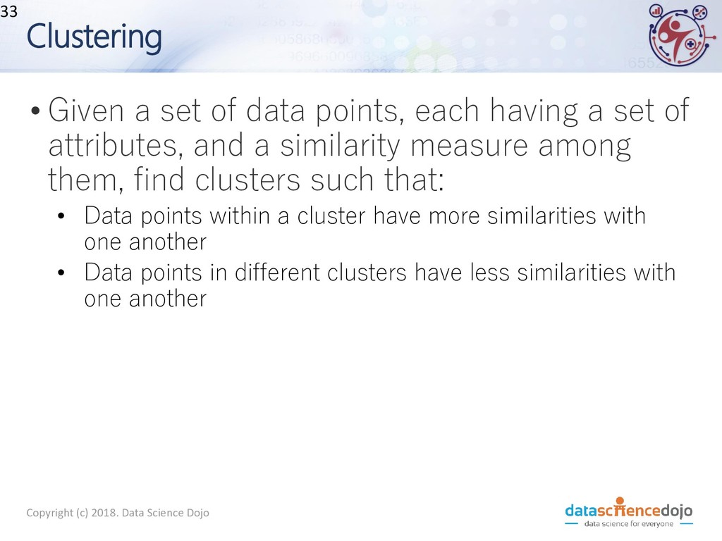
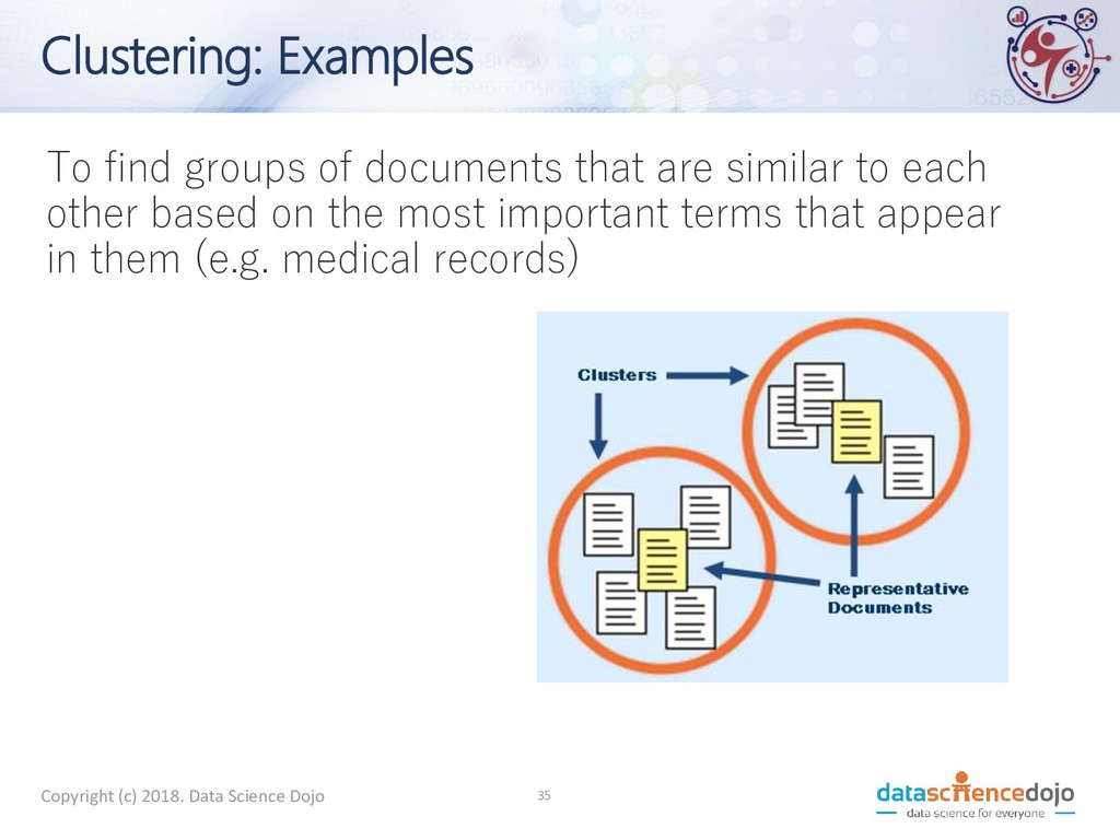
a set of attributes, and a similarity measure among them, find clusters such that: • Data points within a cluster have more similarities with one another • Data points in different clusters have less similarities with one another 33 Copyright (c) 2018. Data Science Dojo
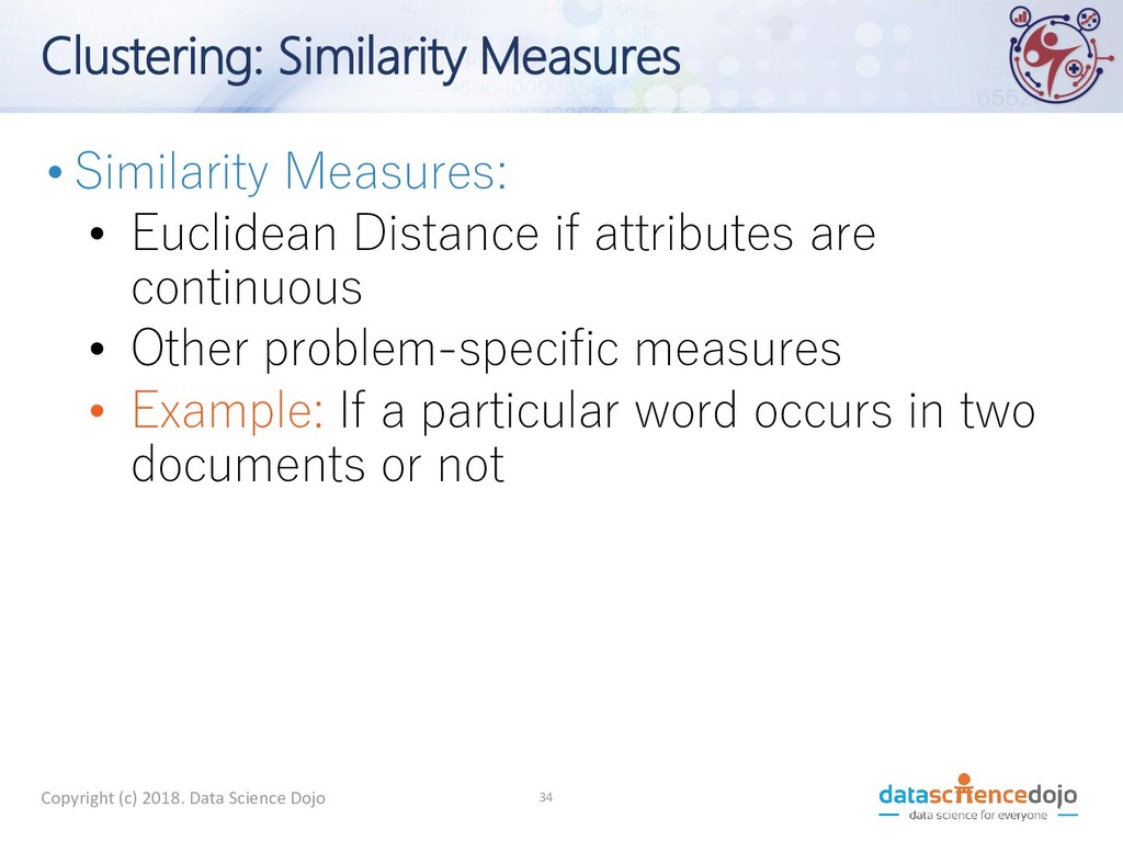
attributes are continuous • Other problem-specific measures • Example: If a particular word occurs in two documents or not Copyright (c) 2018. Data Science Dojo 34
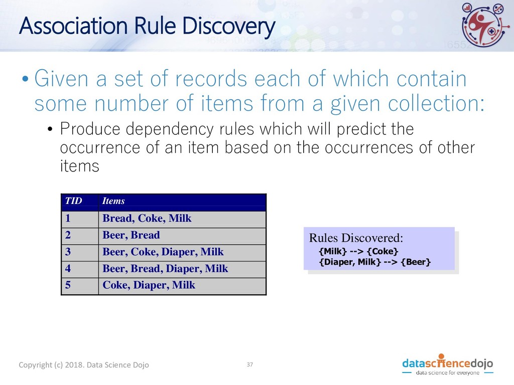
of which contain some number of items from a given collection: • Produce dependency rules which will predict the occurrence of an item based on the occurrences of other items TID Items 1 Bread, Coke, Milk 2 Beer, Bread 3 Beer, Coke, Diaper, Milk 4 Beer, Bread, Diaper, Milk 5 Coke, Diaper, Milk Rules Discovered: {Milk} --> {Coke} {Diaper, Milk} --> {Beer} Copyright (c) 2018. Data Science Dojo 37
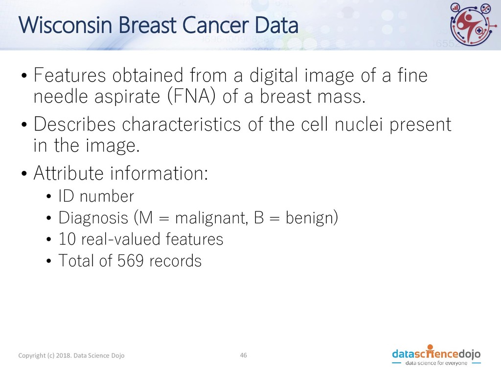
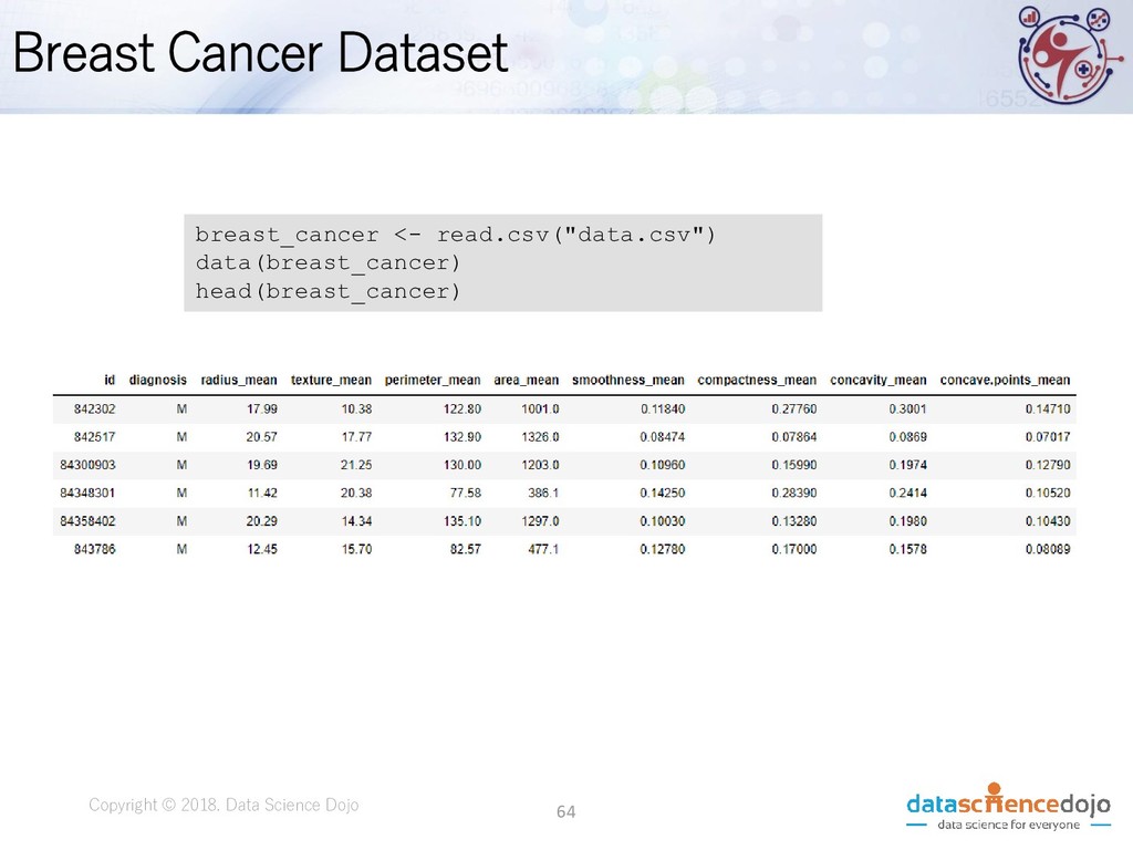
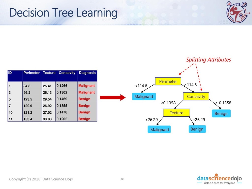
Dojo • Features obtained from a digital image of a fine needle aspirate (FNA) of a breast mass. • Describes characteristics of the cell nuclei present in the image. • Attribute information: • ID number • Diagnosis (M = malignant, B = benign) • 10 real-valued features • Total of 569 records
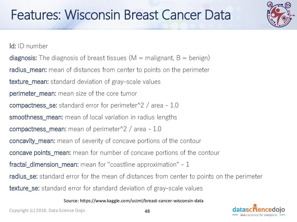
Science Dojo Id: ID number diagnosis: The diagnosis of breast tissues (M = malignant, B = benign) radius_mean: mean of distances from center to points on the perimeter texture_mean: standard deviation of gray-scale values perimeter_mean: mean size of the core tumor compactness_se: standard error for perimeter^2 / area - 1.0 smoothness_mean: mean of local variation in radius lengths compactness_mean: mean of perimeter^2 / area - 1.0 concavity_mean: mean of severity of concave portions of the contour concave points_mean: mean for number of concave portions of the contour fractal_dimension_mean: mean for "coastline approximation" - 1 radius_se: standard error for the mean of distances from center to points on the perimeter texture_se: standard error for standard deviation of gray-scale values Source: https://www.kaggle.com/uciml/breast-cancer-wisconsin-data
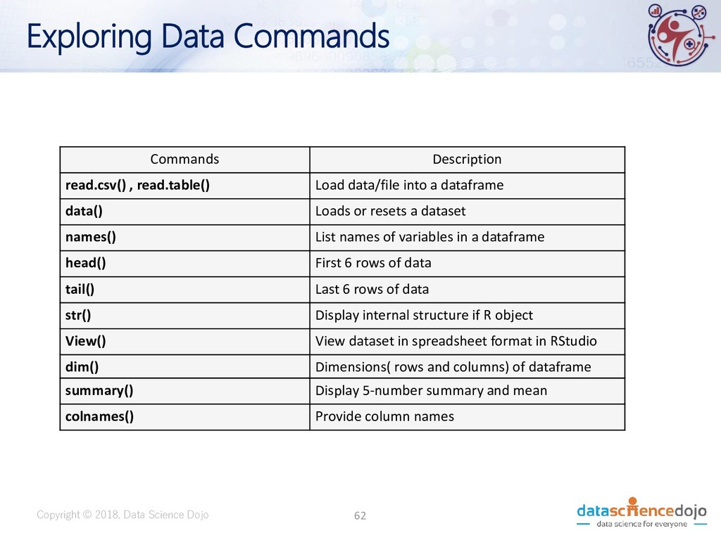
Description read.csv() , read.table() Load data/file into a dataframe data() Loads or resets a dataset names() List names of variables in a dataframe head() First 6 rows of data tail() Last 6 rows of data str() Display internal structure if R object View() View dataset in spreadsheet format in RStudio dim() Dimensions( rows and columns) of dataframe summary() Display 5-number summary and mean colnames() Provide column names 62
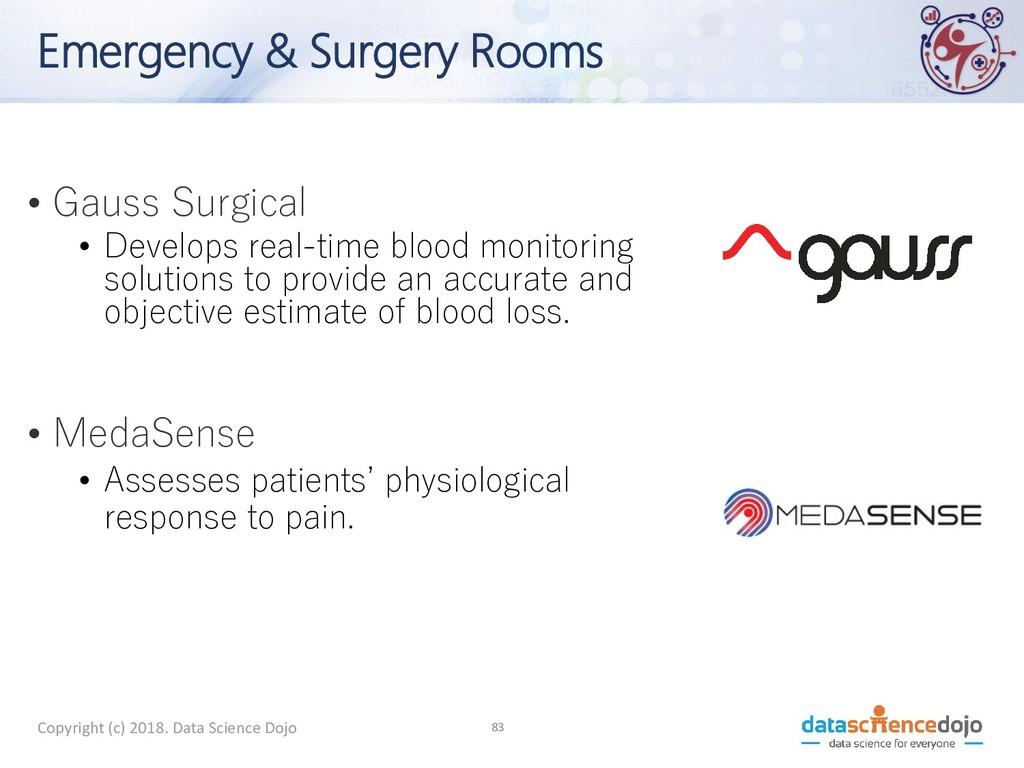
Surgery Rooms • Gauss Surgical • Develops real-time blood monitoring solutions to provide an accurate and objective estimate of blood loss. • MedaSense • Assesses patients’ physiological response to pain.
& Risk Assessment ▪ Watson for oncology • Analyzes patients medical records and identify treatment options for doctors and patients. ▪ SkinVision • Assesses skin cancer risk using image recognition and user provided information. ▪ Berg • Includes dosage trials for intravenous tumor treatment, detection and management of prostate cancer.
▪ MedyMatch • Helps treat stroke and head trauma more effectively by detecting intracranial brain bleeds. ▪ P1vital • Predicting Response to Depression Treatment (PReDicT test) uses Machine Learning to provide anti- depressant treatment.
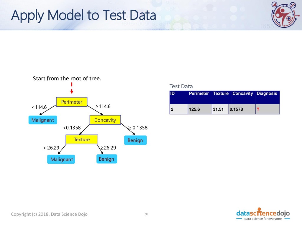
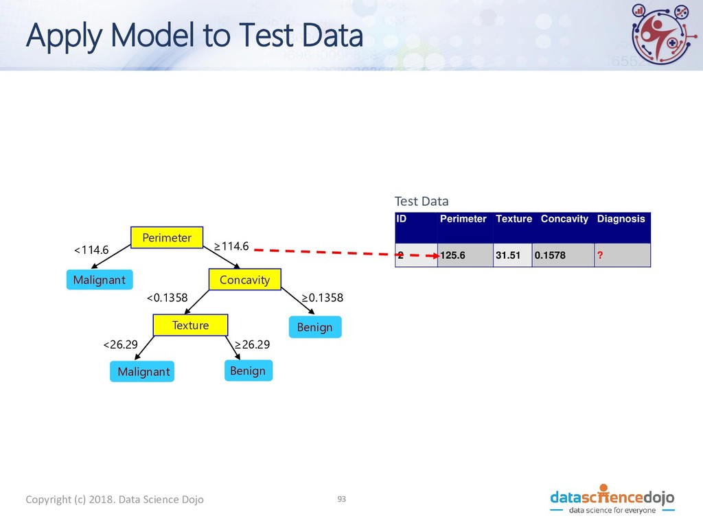
to Test Data Test Data Start from the root of tree. Perimeter Concavity Texture Benign Malignant Malignant Benign <114.6 ≥114.6 ≥ 0.1358 <0.1358 < 26.29 ≥26.29 ID Perimeter Texture Concavity Diagnosis 2 125.6 31.51 0.1578 ? 10
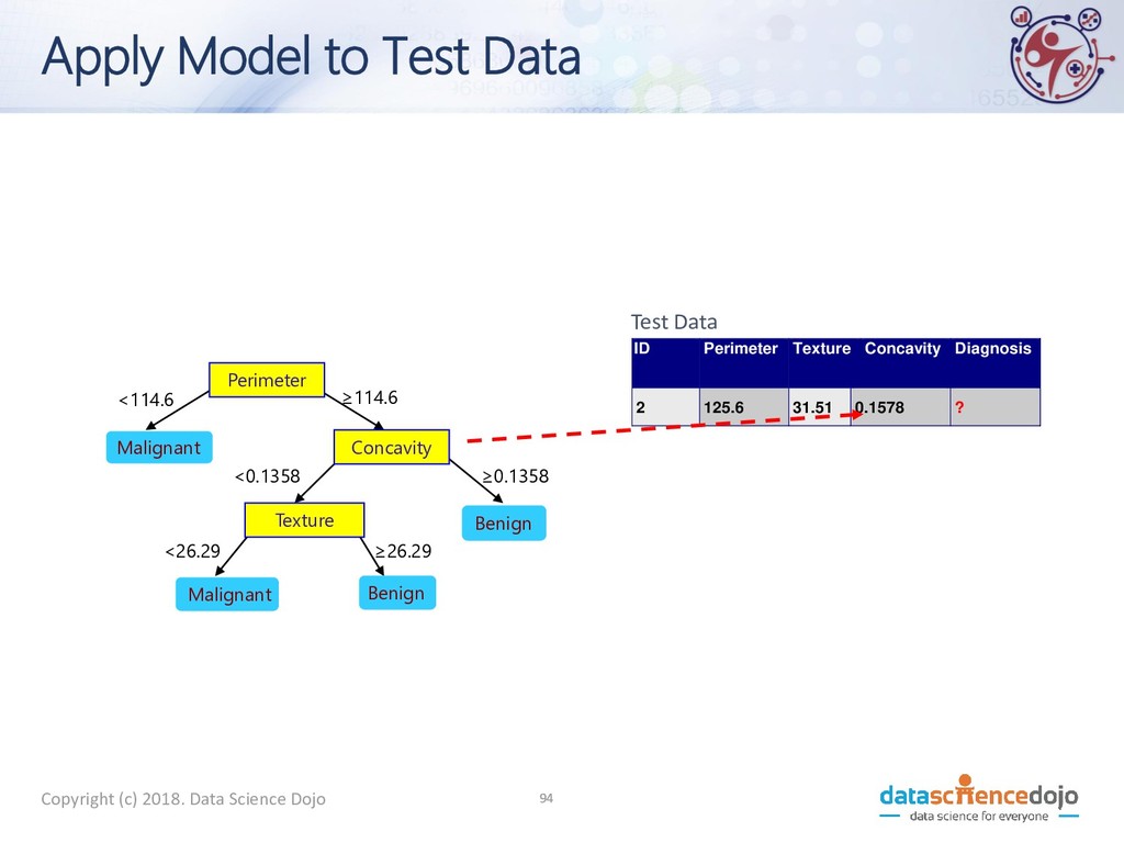
to Test Data Test Data Perimeter Concavity Texture Benign Malignant Malignant Benign <114.6 ≥114.6 ≥0.1358 <0.1358 <26.29 ≥26.29 ID Perimeter Texture Concavity Diagnosis 2 125.6 31.51 0.1578 ? 10
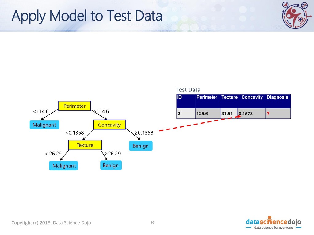
to Test Data Test Data Perimeter Concavity Texture Benign Malignant Malignant Benign <114.6 ≥114.6 ≥0.1358 <0.1358 <26.29 ≥26.29 ID Perimeter Texture Concavity Diagnosis 2 125.6 31.51 0.1578 ? 10
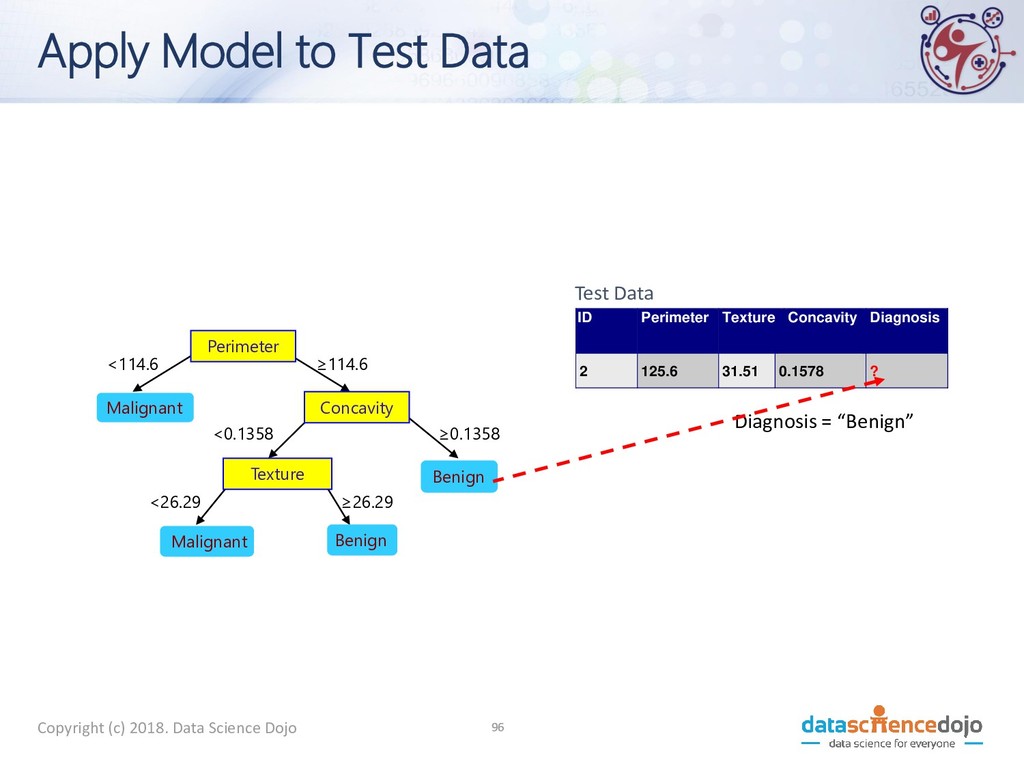
to Test Data Test Data Perimeter Concavity Texture Benign Malignant Malignant Benign <114.6 ≥114.6 ≥0.1358 <0.1358 <26.29 ≥26.29 ID Perimeter Texture Concavity Diagnosis 2 125.6 31.51 0.1578 ? 10
to Test Data Test Data Perimeter Concavity Texture Benign Malignant Malignant Benign <114.6 ≥114.6 ≥0.1358 <0.1358 < 26.29 ≥26.29 ID Perimeter Texture Concavity Diagnosis 2 125.6 31.51 0.1578 ? 10
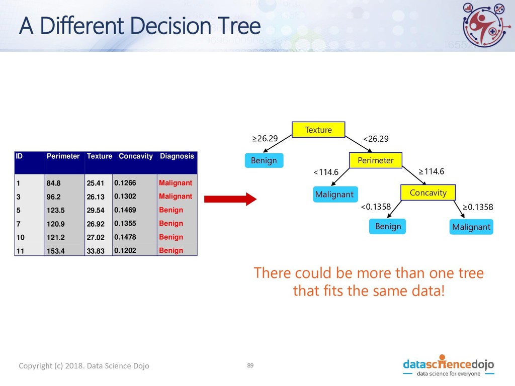
We Get A Tree? • Exponentially many decision trees are possible • Finding the optimal tree is infeasible • Greedy methods that find near-optimal solutions do exist
• Greedy strategy • Split based attribute test that optimizes a criterion • Issues • How to split the records • What attribute test condition? • How to determine the best split? • When do we stop?
• Greedy strategy • Split based attribute test that optimizes a criterion • Issues • How to split the records • What attribute test criterion? • How to determine the best split? • When do we stop?
• Greedy strategy • Split based attribute test that optimizes a criterion • Issues • How to split the records • What attribute test criterion? • How to determine the best split? • When do we stop?
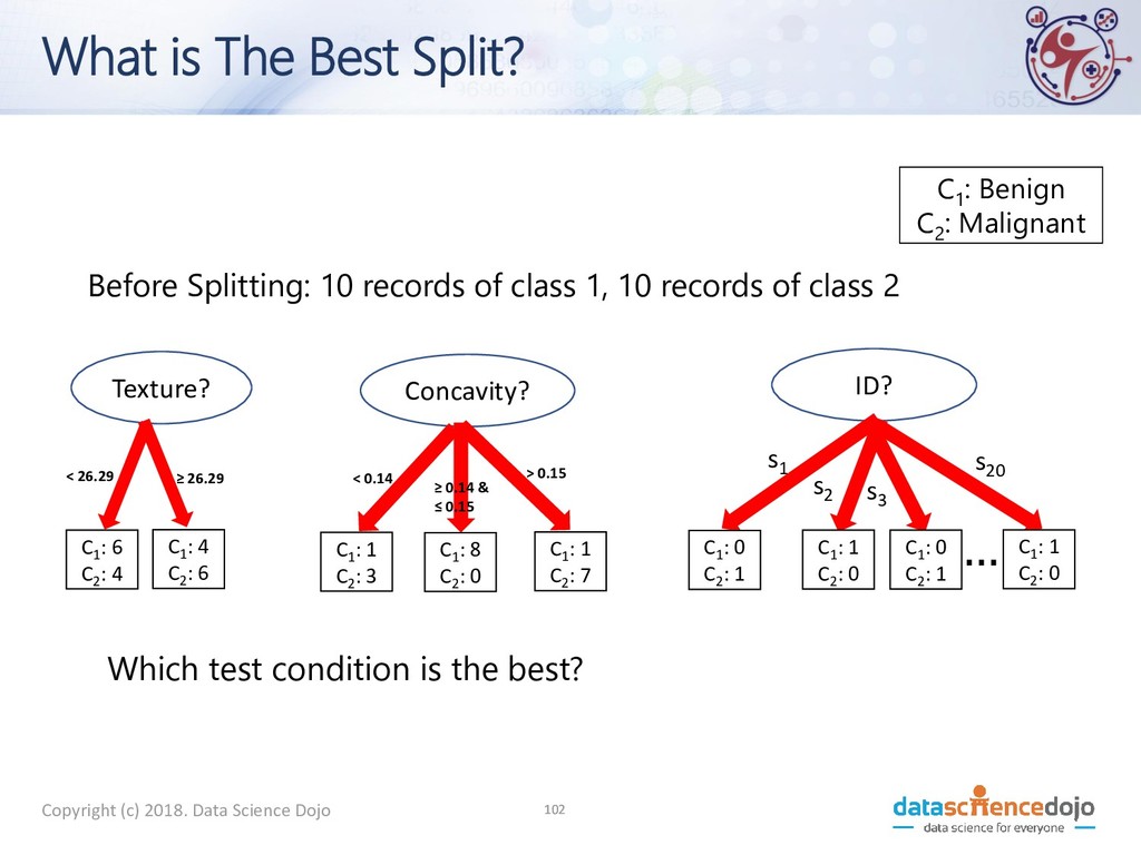
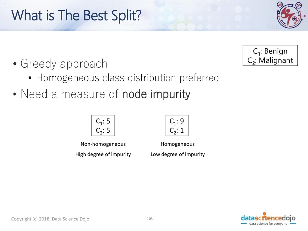
9 C2 : 1 C1 : 5 C2 : 5 What is The Best Split? • Greedy approach • Homogeneous class distribution preferred • Need a measure of node impurity Non-homogeneous High degree of impurity Homogeneous Low degree of impurity C1 : Benign C2 : Malignant
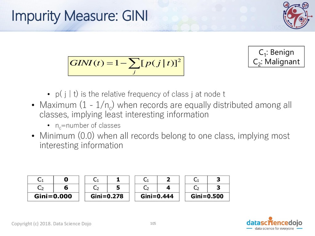
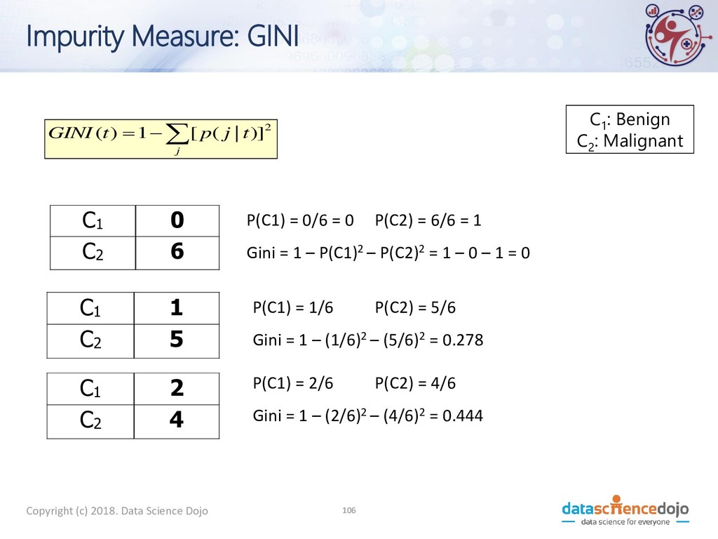
GINI • p( j | t) is the relative frequency of class j at node t • Maximum (1 - 1/n c ) when records are equally distributed among all classes, implying least interesting information • n c =number of classes • Minimum (0.0) when all records belong to one class, implying most interesting information − = j t j p t GINI 2 )] | ( [ 1 ) ( C1 0 C2 6 Gini=0.000 C1 2 C2 4 Gini=0.444 C1 3 C2 3 Gini=0.500 C1 1 C2 5 Gini=0.278 C1 : Benign C2 : Malignant
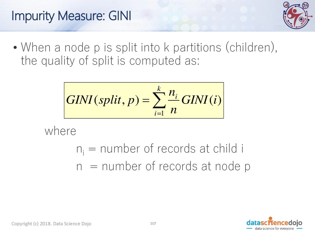
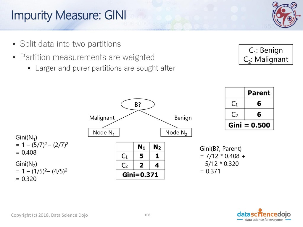
GINI • When a node p is split into k partitions (children), the quality of split is computed as: where n i = number of records at child i n = number of records at node p = = k i i i GINI n n p split GINI 1 ) ( ) , (
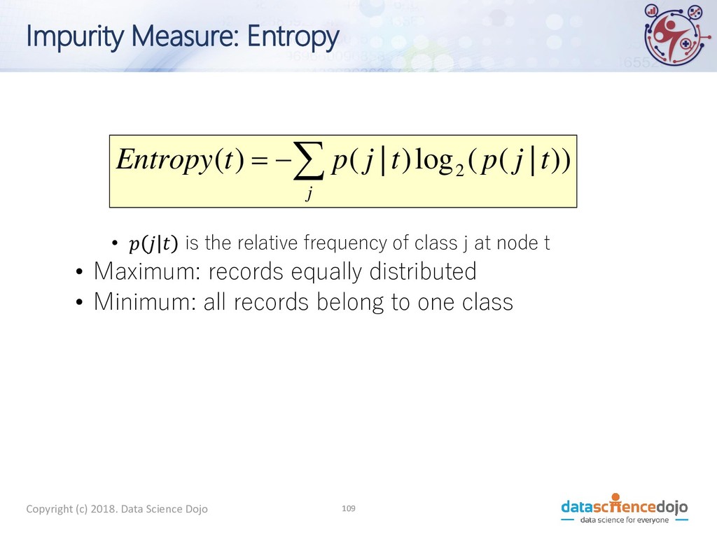
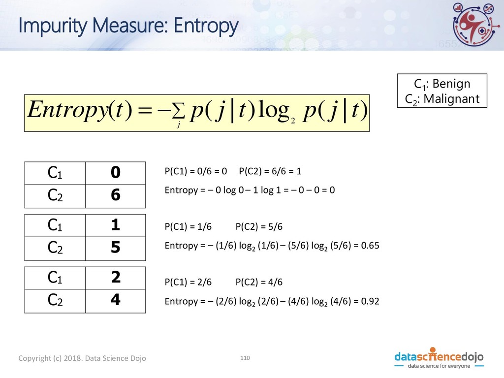
the relative frequency of class j at node t • Maximum: records equally distributed • Minimum: all records belong to one class − = j t j p t j p t Entropy )) | ( ( log ) | ( ) ( 2 Impurity Measure: Entropy
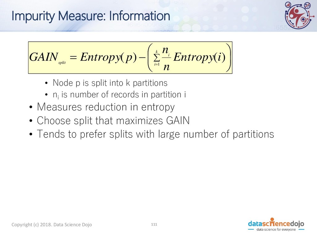
Information • Node p is split into k partitions • n i is number of records in partition i • Measures reduction in entropy • Choose split that maximizes GAIN • Tends to prefer splits with large number of partitions − = = k i i split i Entropy n n p Entropy GAIN 1 ) ( ) (
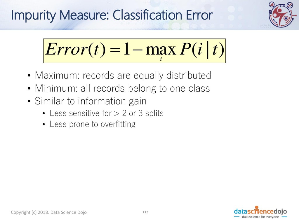
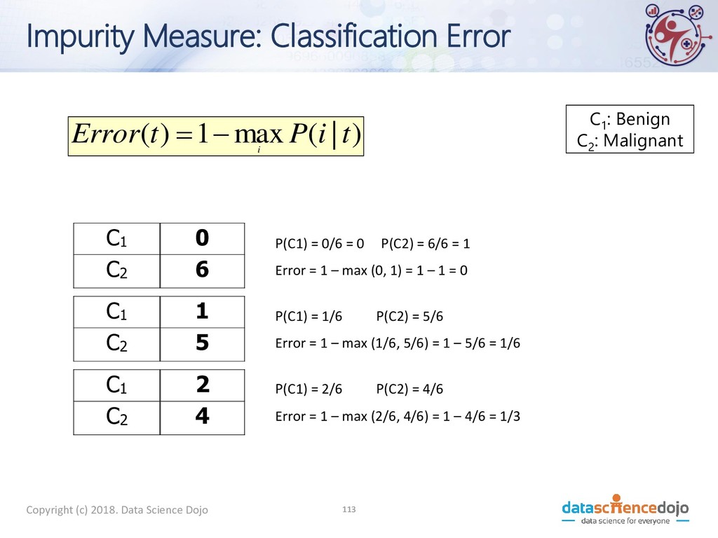
Classification Error • Maximum: records are equally distributed • Minimum: all records belong to one class • Similar to information gain • Less sensitive for > 2 or 3 splits • Less prone to overfitting ) | ( max 1 ) ( t i P t Error i − =
• Greedy strategy • Split based attribute test that optimizes a criterion • Issues • How to split the records • What attribute test criterion? • How to determine the best split? • When do we stop?
Criteria • All the records belong to the same class • All the records have similar attribute values • Fixed termination or pruning • Number of Levels • Number in Leaf Node • Minimum samples per leaf node
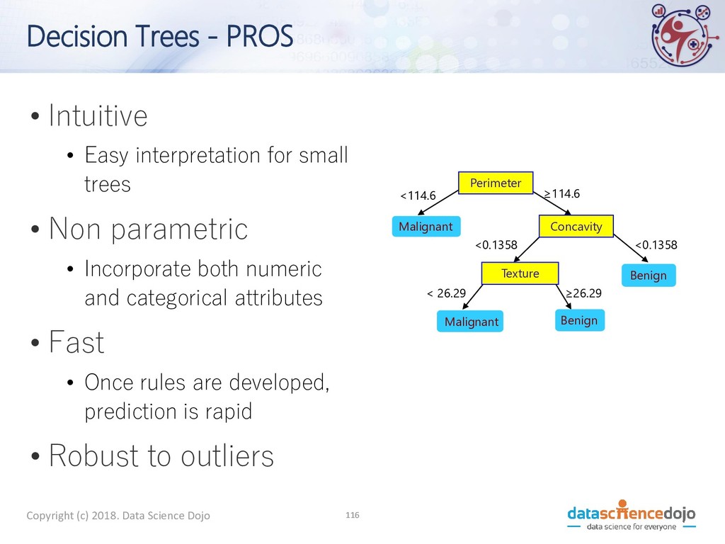
- PROS • Intuitive • Easy interpretation for small trees • Non parametric • Incorporate both numeric and categorical attributes • Fast • Once rules are developed, prediction is rapid • Robust to outliers Perimeter Concavity Texture Benign Malignant Malignant Benign <114.6 ≥114.6 <0.1358 <0.1358 < 26.29 ≥26.29
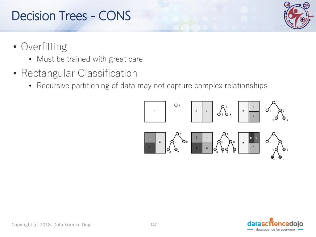
- CONS • Overfitting • Must be trained with great care • Rectangular Classification • Recursive partitioning of data may not capture complex relationships
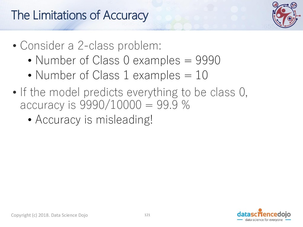
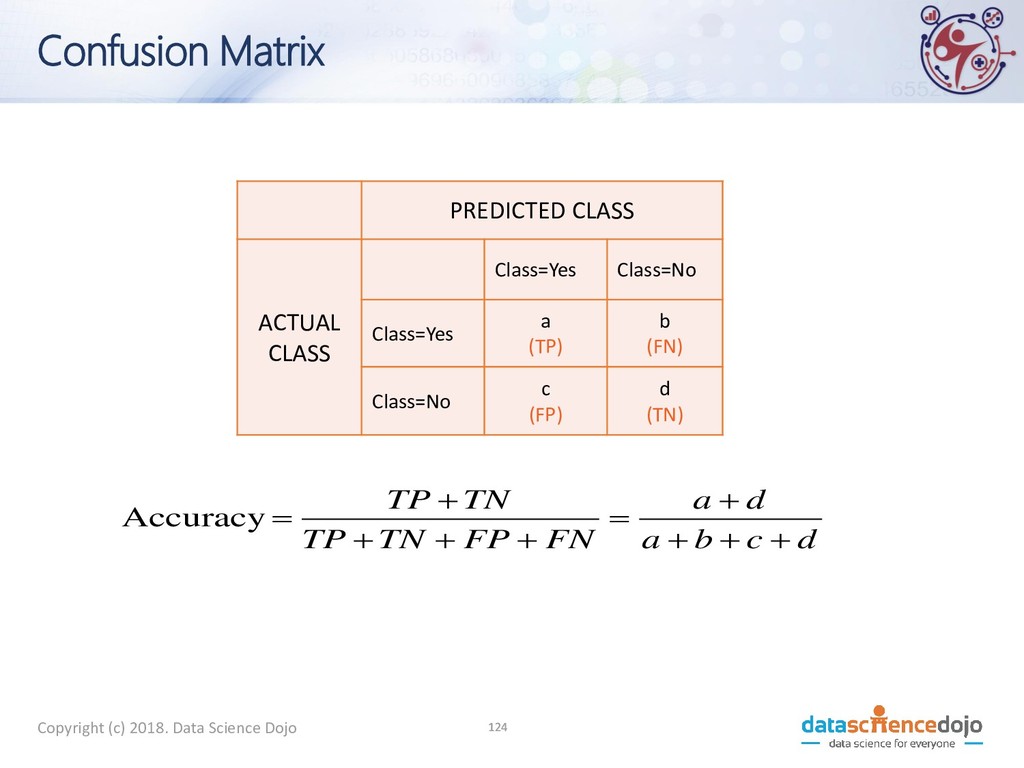
of Accuracy • Consider a 2-class problem: • Number of Class 0 examples = 9990 • Number of Class 1 examples = 10 • If the model predicts everything to be class 0, accuracy is 9990/10000 = 99.9 % • Accuracy is misleading!
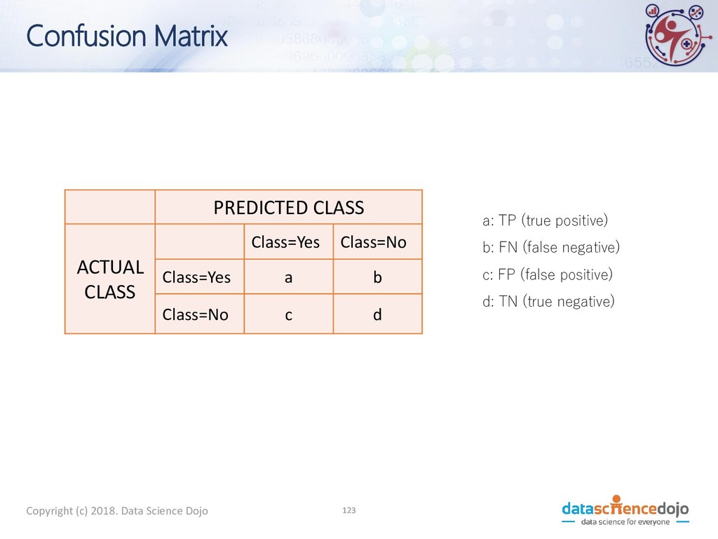
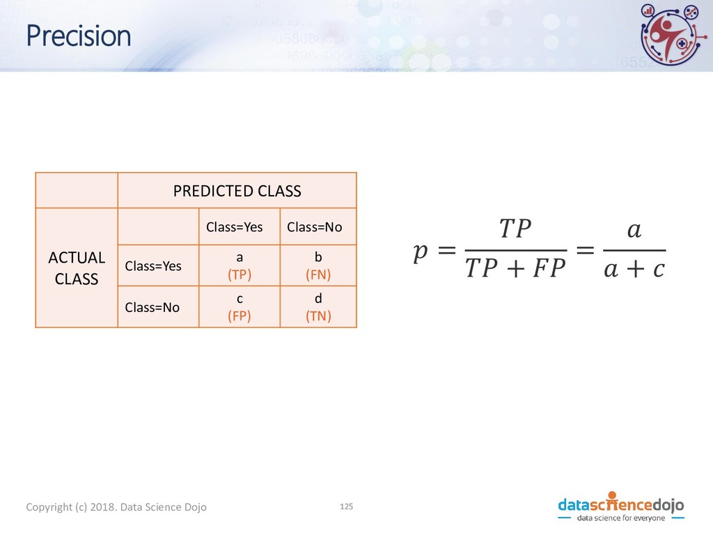
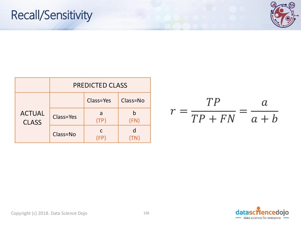
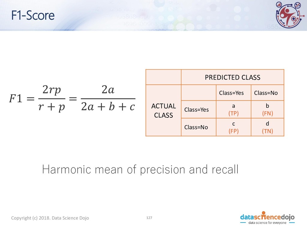
PREDICTED CLASS ACTUAL CLASS Class=Yes Class=No Class=Yes a b Class=No c d a: TP (true positive) b: FN (false negative) c: FP (false positive) d: TN (true negative)
PREDICTED CLASS ACTUAL CLASS Class=Yes Class=No Class=Yes a (TP) b (FN) Class=No c (FP) d (TN) d c b a d a FN FP TN TP TN TP + + + + = + + + + = Accuracy
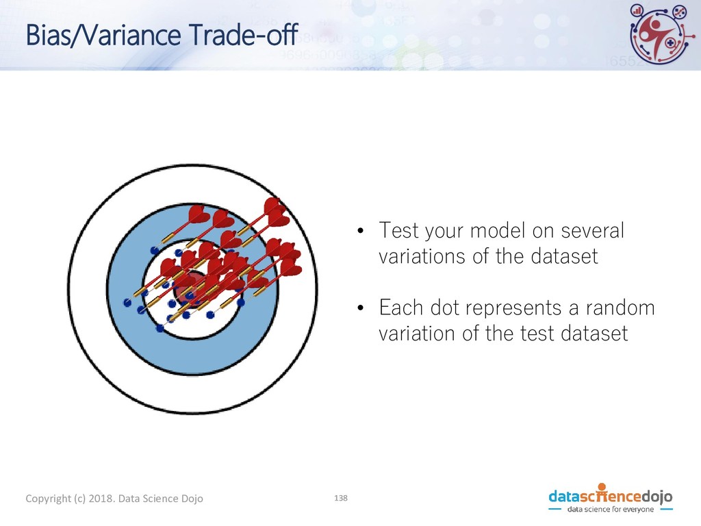
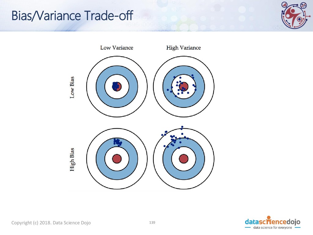
A machine learning model should be able to handle any data set coming from the same distribution as the training set. • Generalization refers to a model's ability to handle any random variations of training data
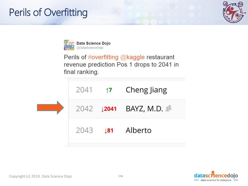
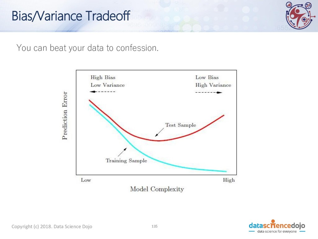
of generalization) • The gravest and most common sin of machine learning • Overfitting: learning so much from your data that you memorize it. • You do well on training data • But don’t do well (or even fail miserably) on test data
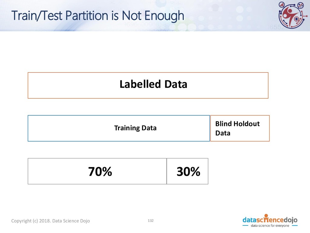
Dataset • The person building the model has no access to the blind holdout dataset • Why do we need to lock it away? • Even in presence of a 70/30 split, you may end up with a model that is not generalized
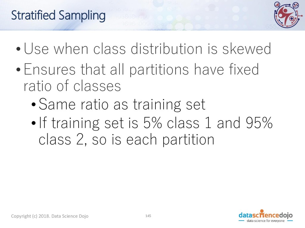
•Use when class distribution is skewed •Ensures that all partitions have fixed ratio of classes •Same ratio as training set • If training set is 5% class 1 and 95% class 2, so is each partition
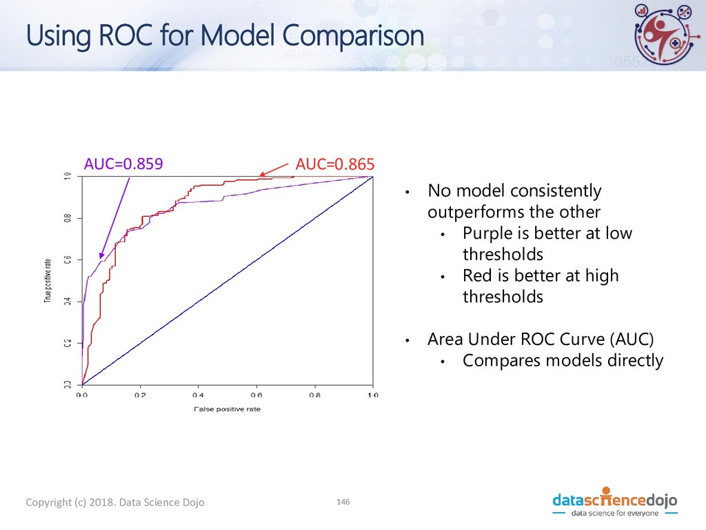
for Model Comparison • No model consistently outperforms the other • Purple is better at low thresholds • Red is better at high thresholds • Area Under ROC Curve (AUC) • Compares models directly AUC=0.865 AUC=0.859
![Traffic Management Descriptive [Informing Role]: • Traffic jam has happened](https://files.speakerdeck.com/presentations/6766bd9bd21f4b2fa6cd2fcbe5a99330/slide_24.jpg)
![Traffic Management Predictive [Informing and Warning Role]: • Traffic jam](https://files.speakerdeck.com/presentations/6766bd9bd21f4b2fa6cd2fcbe5a99330/slide_25.jpg)
![Traffic Management Prescriptive [Informing, Warning, and Advisory Role]: Take action](https://files.speakerdeck.com/presentations/6766bd9bd21f4b2fa6cd2fcbe5a99330/slide_26.jpg)