リエナール_ヴィーヘルト_ポテンシャルの導出と回転する双極子の可視化について.pdf

Transcript

1. リエナール・ヴィーヘルト・ポテンシャルの 導出について
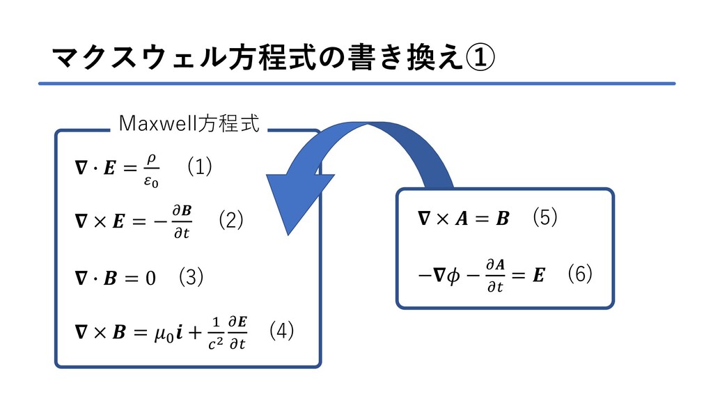
2. マクスウェル方程式の書き換え① ∙ = 0 (1) × = − (2) ∙ = 0 (3) × = 0 + 1 2 (4) Maxwell方程式 × = (5) − − = (6)
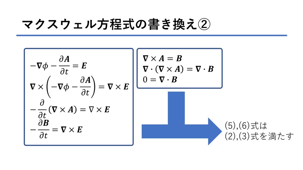
3. マクスウェル方程式の書き換え② × = ∙ × = ∙ 0 = ∙ − − = × − − = × − × = ∇ × − = × (5),(6)式は (2),(3)式を満たす
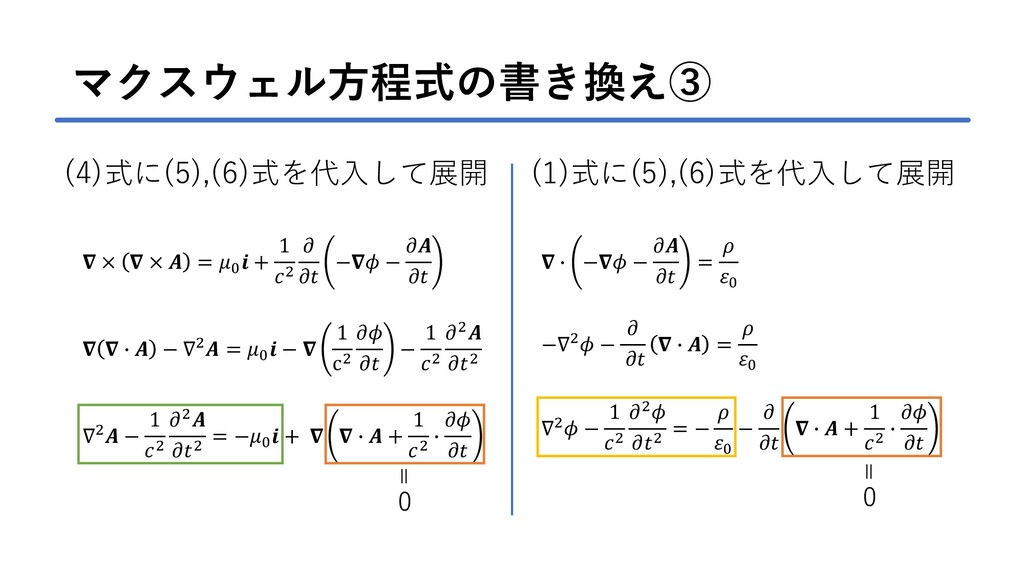
4. マクスウェル方程式の書き換え③ (4)式に(5),(6)式を代入して展開 × × = 0 + 1 2 − − ∙ − ∇2 = 0 − 1 c2 − 1 2 2 2 ∇2 − 1 2 2 2 = −0 + ∙ + 1 2 ∙ (1)式に(5),(6)式を代入して展開 ∙ − − = 0 −∇2 − ∙ = 0 ∇2 − 1 2 2 2 = − 0 − ∙ + 1 2 ∙ = 0 = 0
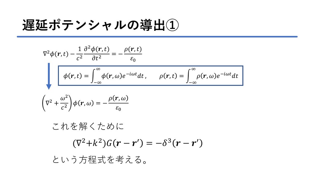
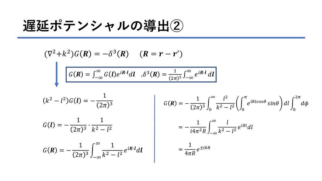
5. 遅延ポテンシャルの導出① ∇2(, ) − 1 2 2(, ) 2 = − (, ) 0 , = න −∞ ∞ , − , , = න −∞ ∞ , − ∇2 + 2 2 , = − , 0 これを解くために (∇2+2) − ′ = −3 − ′ という方程式を考える。
6. 遅延ポテンシャルの導出② (∇2+2) = −3 ( = − ′) = ׬ −∞ ∞ ∙ ,3 = 1 2 3 ׬ −∞ ∞ ∙ 2 − 2 = − 1 2 3 = − 1 2 3 ∙ 1 2 − 2 = − 1 2 3 න −∞ ∞ 1 2 − 2 ∙ = − 1 2 3 න 0 ∞ 2 2 − 2 න 0 න 0 2 = − 1 42 න −∞ ∞ 2 − 2 = 1 4 ±
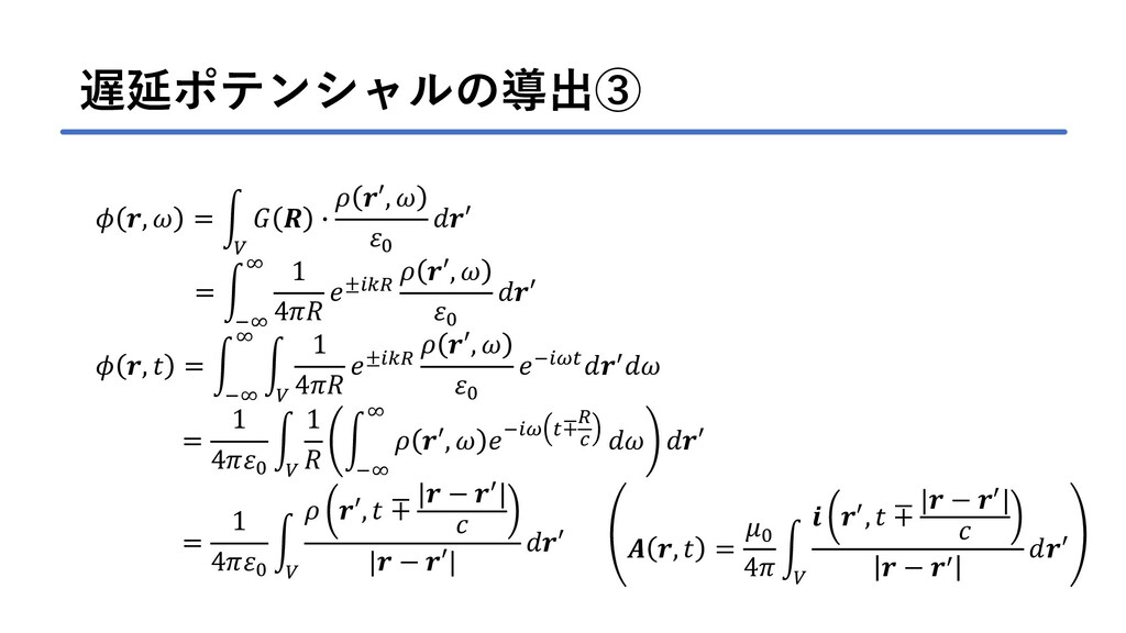
7. 遅延ポテンシャルの導出③ , = න ∙ ′, 0 ′ = න −∞ ∞ 1 4 ± ′, 0 ′ , = න −∞ ∞ න 1 4 ± ′, 0 −′ = 1 40 න 1 න −∞ ∞ ′, − ∓ ′ = 1 40 න ′, ∓ | − ′| | − ′| ′ , = 0 4 න ′, ∓ | − ′| − ′ ′
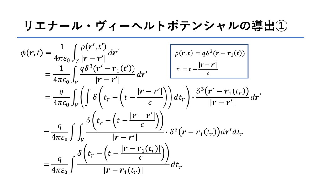
8. リエナール・ヴィーヘルトポテンシャルの導出① , = 1 40 න ′, ′ | − ′| ′ = 1 40 න 3(′ − 1 ′ ) | − ′| ′ = 40 න න − − − ′ ∙ 3 ′ − 1 − ′ ′ = 40 න න − − − ′ − ′ ∙ 3 − 1 ′ = 40 න − − − 1 | − 1 ( )| , = 3( − 1 ) ′ = − − ′
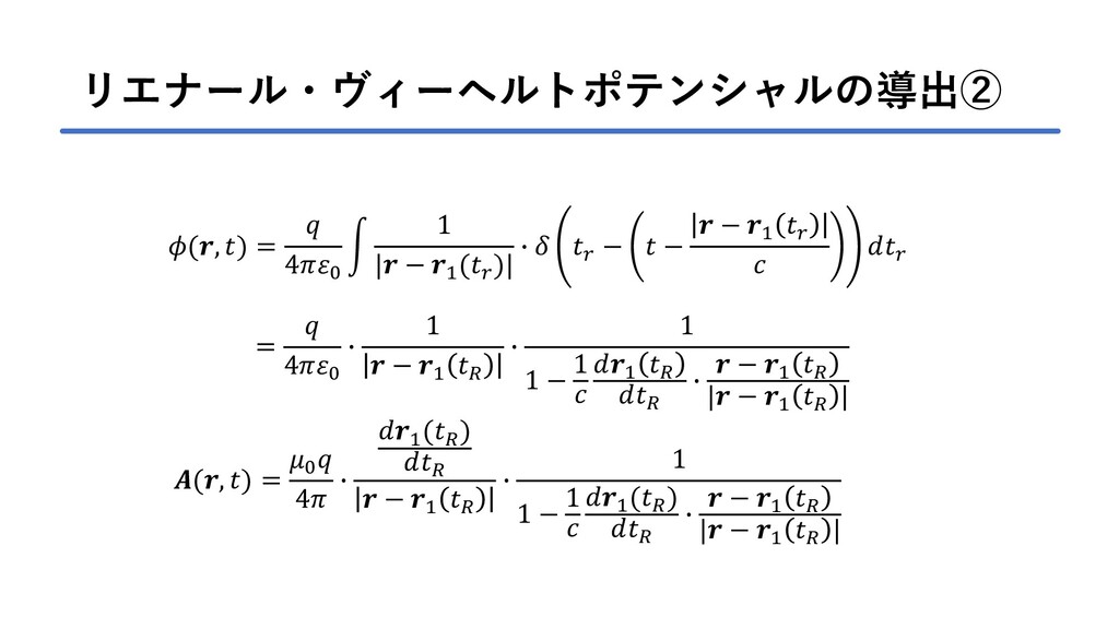
9. リエナール・ヴィーヘルトポテンシャルの導出② = 40 ∙ 1 − 1 ∙ 1 1 − 1 1 ∙ − 1 | − 1 | (, ) = 40 න 1 | − 1 ( )| ∙ − − − 1 (, ) = 0 4 ∙ 1 ( ) − 1 ∙ 1 1 − 1 1 ( ) ∙ − 1 | − 1 |
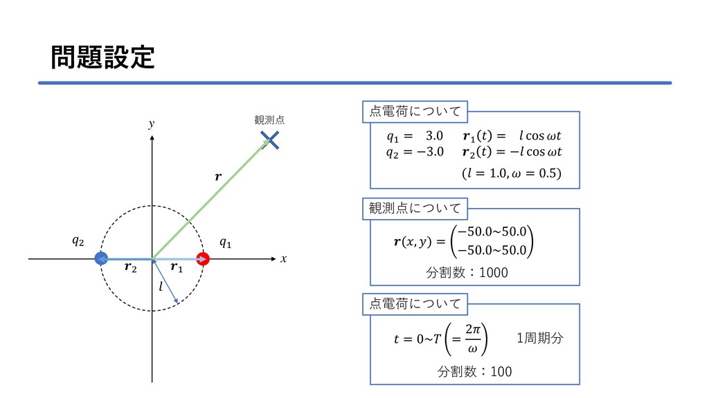
10. 問題設定 y x 1 2 2 観測点 1 (, ) = −50.0~50.0 −50.0~50.0 1 = 3.0 2 = −3.0 1 = cos 2 = − cos ( = 1.0, = 0.5) 点電荷について 観測点について 分割数：1000 点電荷について = 0~ = 2 1周期分 分割数：100
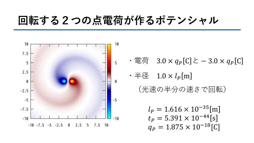
11. 回転する２つの点電荷が作るポテンシャル = 1.616 × 10−35 m = 5.391 × 10−44 s = 1.875 × 10−18[C] ・電荷 3.0 × C と − 3.0 × C ・半径 1.0 × m （光速の半分の速さで回転）