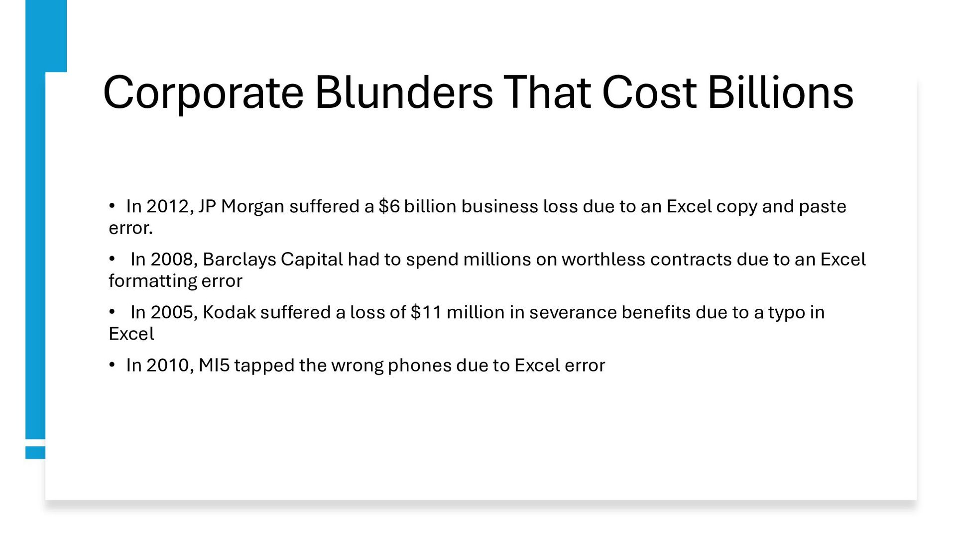
suffered a $6 billion business loss due to an Excel copy and paste error. • In 2008, Barclays Capital had to spend millions on worthless contracts due to an Excel formatting error • In 2005, Kodak suffered a loss of $11 million in severance benefits due to a typo in Excel • In 2010, MI5 tapped the wrong phones due to Excel error
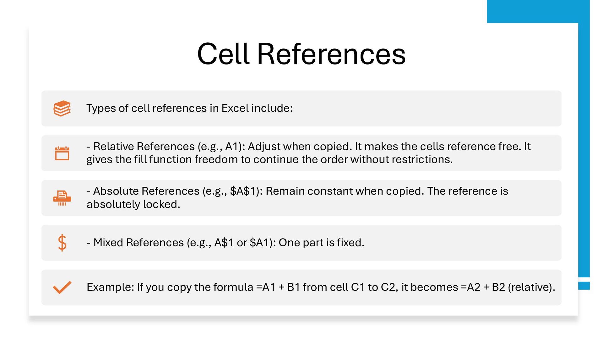
Relative References (e.g., A1): Adjust when copied. It makes the cells reference free. It gives the fill function freedom to continue the order without restrictions. - Absolute References (e.g., $A$1): Remain constant when copied. The reference is absolutely locked. - Mixed References (e.g., A$1 or $A1): One part is fixed. Example: If you copy the formula =A1 + B1 from cell C1 to C2, it becomes =A2 + B2 (relative).
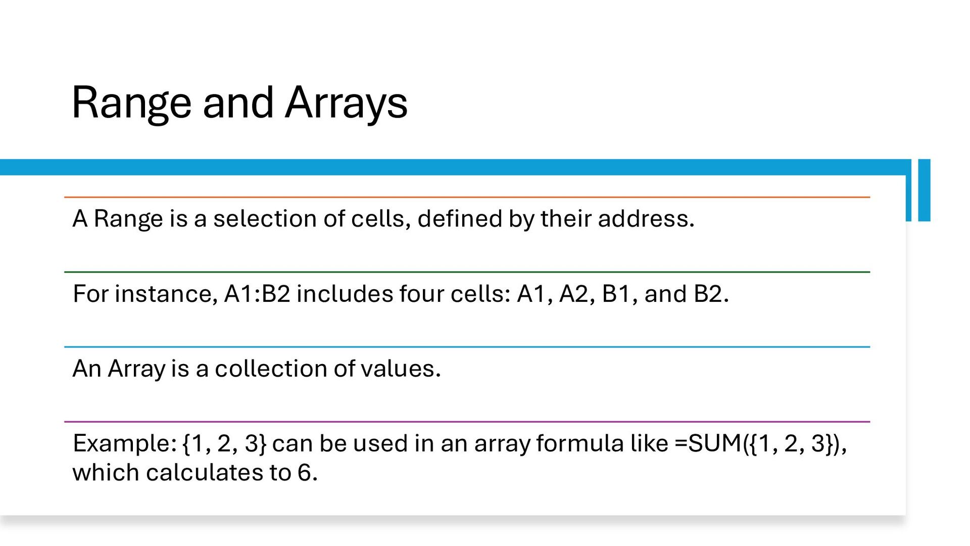
defined by their address. For instance, A1:B2 includes four cells: A1, A2, B1, and B2. An Array is a collection of values. Example: {1, 2, 3} can be used in an array formula like =SUM({1, 2, 3}), which calculates to 6.
a specific range by name instead of cell references. This improves readability and makes formulas easier to manage. Example: Name the range A1:A10 as 'Sales'. You can then use =SUM(Sales) instead of =SUM(A1:A10), making your formulas clearer.
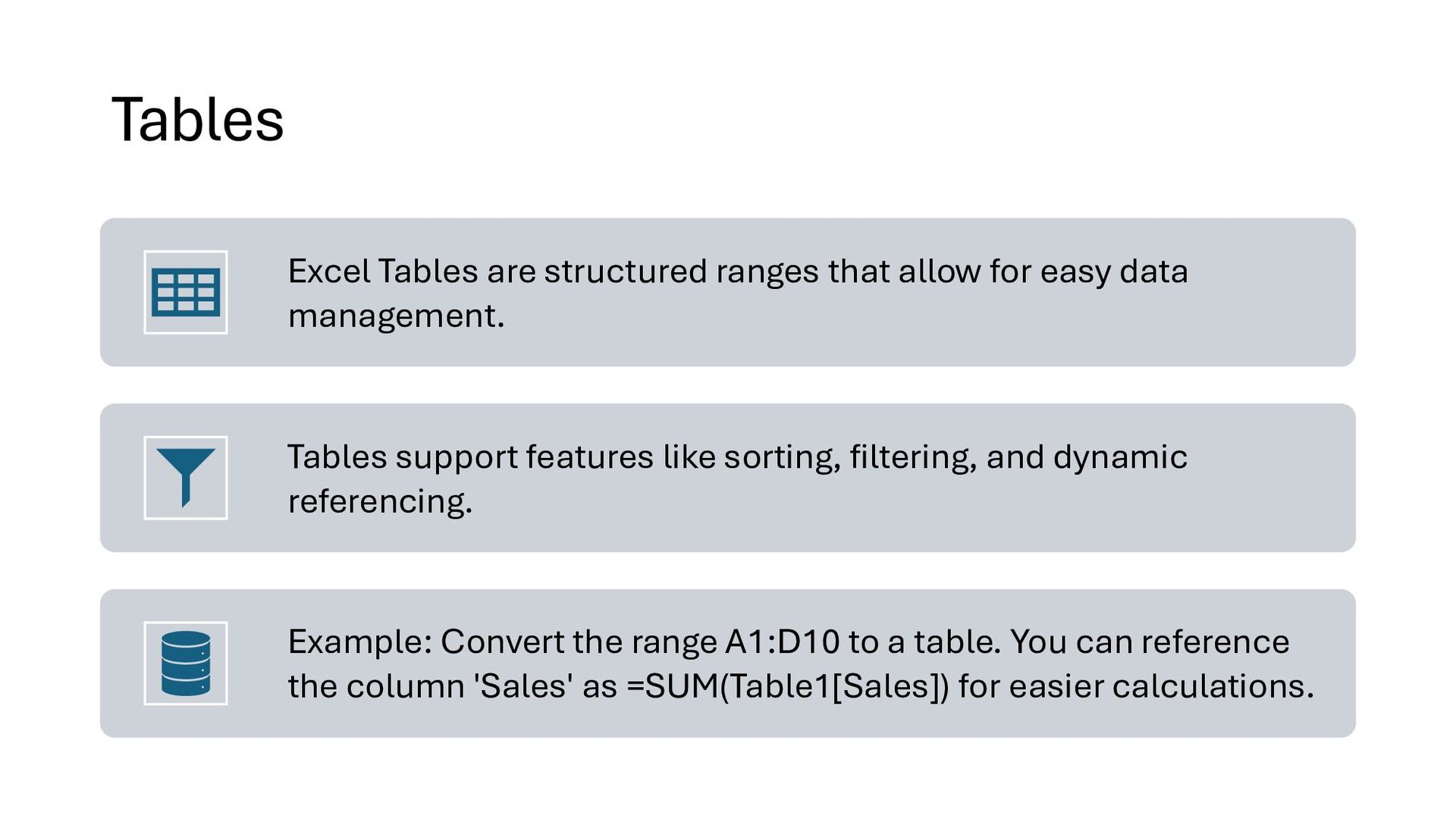
data management. Tables support features like sorting, filtering, and dynamic referencing. Example: Convert the range A1:D10 to a table. You can reference the column 'Sales' as =SUM(Table1[Sales]) for easier calculations.
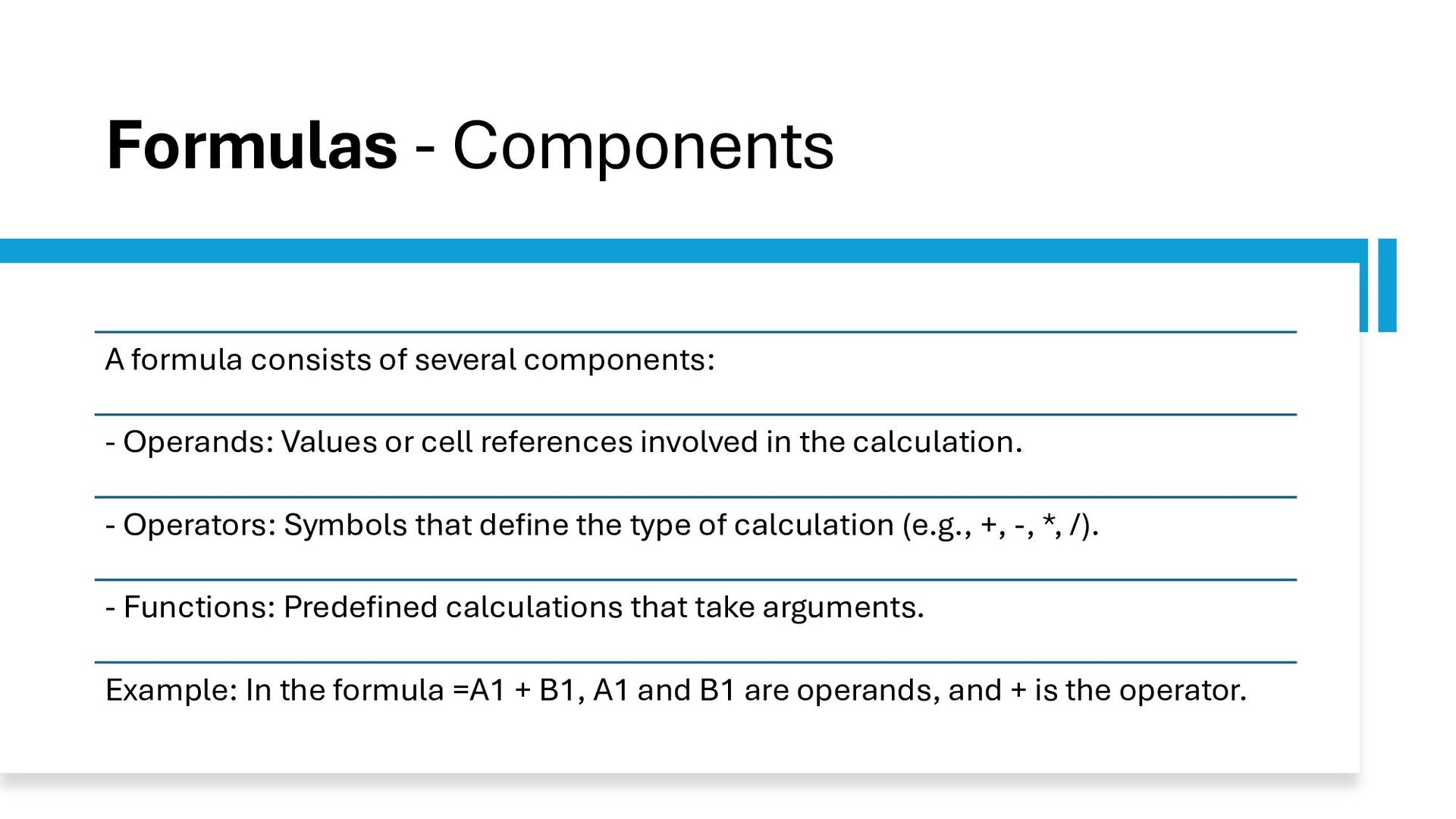
Operands: Values or cell references involved in the calculation. - Operators: Symbols that define the type of calculation (e.g., +, -, *, /). - Functions: Predefined calculations that take arguments. Example: In the formula =A1 + B1, A1 and B1 are operands, and + is the operator.
Operands: Values or cell references involved in the calculation. - Operators: Symbols that define the type of calculation (e.g., +, -, *, /). - Functions: Predefined calculations that take arguments. Example: In the formula =A1 + B1, A1 and B1 are operands, and + is the operator.
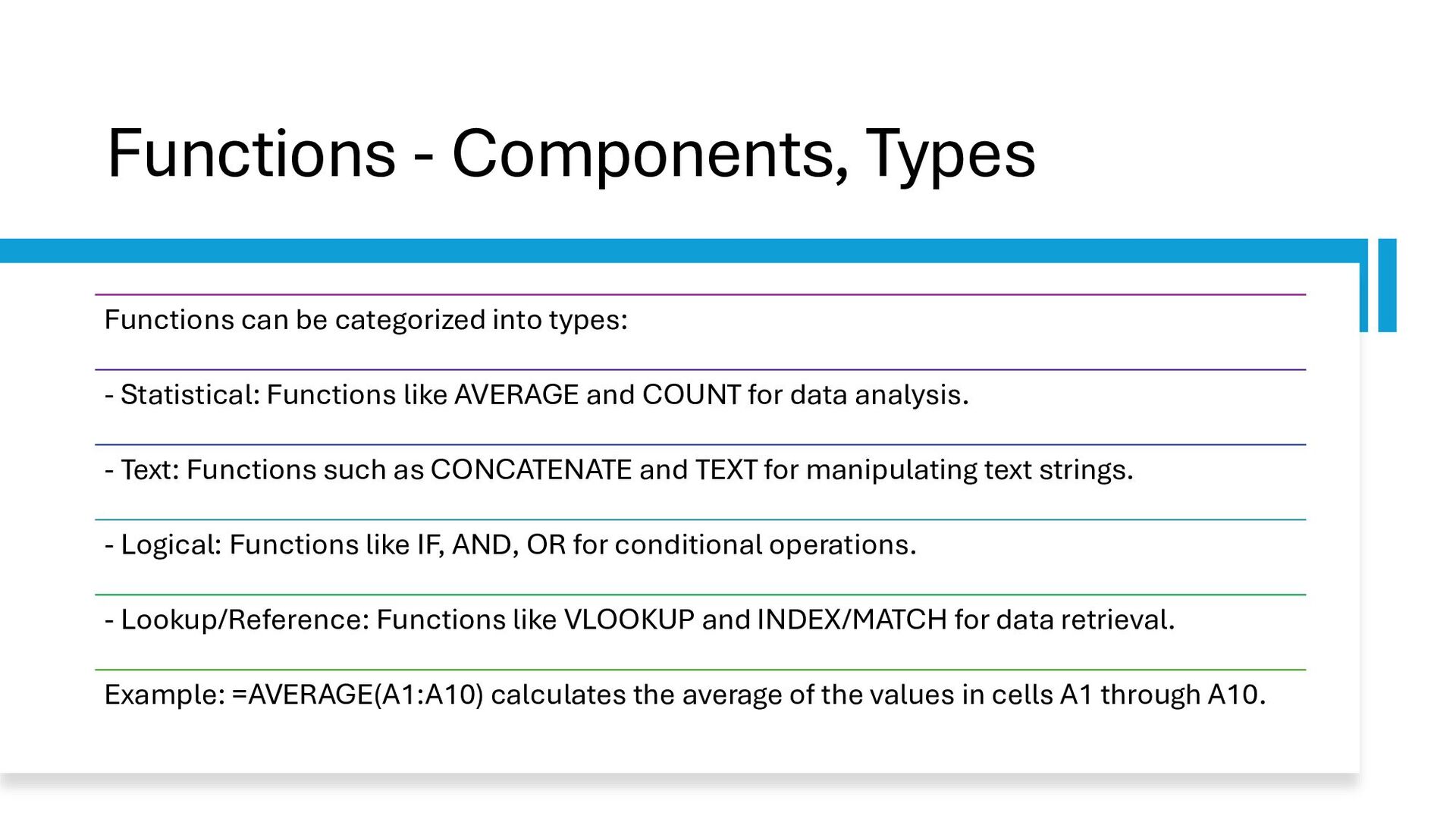
- Statistical: Functions like AVERAGE and COUNT for data analysis. - Text: Functions such as CONCATENATE and TEXT for manipulating text strings. - Logical: Functions like IF, AND, OR for conditional operations. - Lookup/Reference: Functions like VLOOKUP and INDEX/MATCH for data retrieval. Example: =AVERAGE(A1:A10) calculates the average of the values in cells A1 through A10.
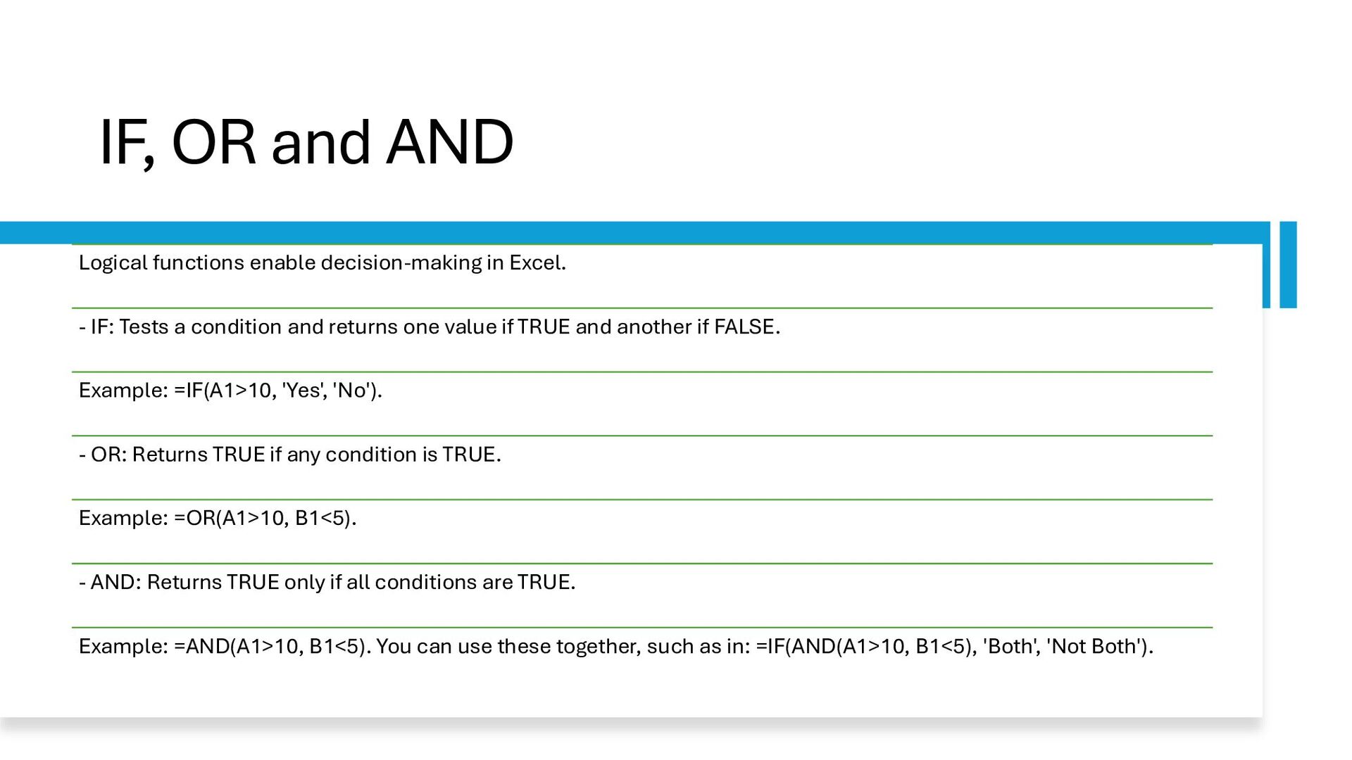
- IF: Tests a condition and returns one value if TRUE and another if FALSE. Example: =IF(A1>10, 'Yes', 'No'). - OR: Returns TRUE if any condition is TRUE. Example: =OR(A1>10, B1<5). - AND: Returns TRUE only if all conditions are TRUE. Example: =AND(A1>10, B1<5). You can use these together, such as in: =IF(AND(A1>10, B1<5), 'Both', 'Not Both').
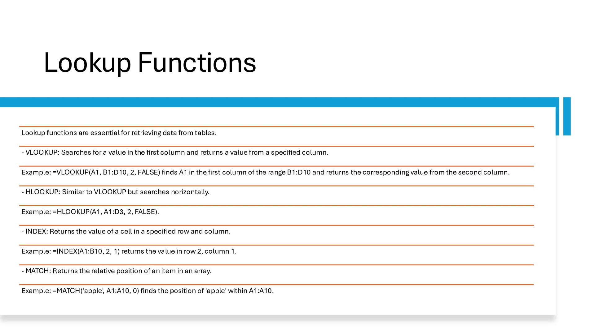
tables. - VLOOKUP: Searches for a value in the first column and returns a value from a specified column. Example: =VLOOKUP(A1, B1:D10, 2, FALSE) finds A1 in the first column of the range B1:D10 and returns the corresponding value from the second column. - HLOOKUP: Similar to VLOOKUP but searches horizontally. Example: =HLOOKUP(A1, A1:D3, 2, FALSE). - INDEX: Returns the value of a cell in a specified row and column. Example: =INDEX(A1:B10, 2, 1) returns the value in row 2, column 1. - MATCH: Returns the relative position of an item in an array. Example: =MATCH('apple', A1:A10, 0) finds the position of 'apple' within A1:A10.