Machine Learning in Genetics

Transcript

1. Machine Learning in Genetics: Lessons Learned Beth Signal @BethSignal b.signal@garvan.org.au
2. Outline Introduction to Machine Learning R code & notebook for coding/noncoding transcript classification. • Types of Machine Learning • When it can be applied to genetic problems Quick guide for creating supervised learning models • Some tips and considerations I wish I’d known about before starting out github.com/betsig/ML_caret_example
3. What is machine learning? Company Application Google Search Optimise search results so ‘best’ results are shown first Facebook Recommend friends and content based on social network and behaviour Netflix Recommend movies based on watch history & behaviour Snapchat Add filters to photos based on facial mapping VPN, Incognito Signed in, location on
4. Types of machine learning Machine Learning Classification Regression Clustering Output is a discrete class Output is continous Output is pattern in the data Supervised Learning Unsupervised Learning Model given input and desired output Model given input Use to make predictions Use to explore data • Gene expression • Time until cancer relapse • Cell type (cancer/normal) • Sequence type (promoter/not) A B A B C A B A B C A B A B C
5. Why use machine learning? Humans vs. computers Problem is ‘complex’ Time/Cost “Big” Datasets 1000’s of genes, interacting No clear linear patterns Radiologists can diagnose pneumonia from chest x-rays Time for radiologist diagnosis > Time for machine diagnosis After 1 month of model training, computer outperforms radiologist Sequencing costs decreasing number of *omes generated increasing How to extract meaningful insights? Rajpurkar et al. 2017. arXiv:1711.05225 Noise within the data
6. Applications of Machine Learning in Genetics Genomic Sequence Class Enhancers Transcription Factor Binding Sites Splice Sites Alternative Splicing Genomic/Transcriptomic State CpG methylation Gene Expression Phenotype Cancer subtypes Drug Response
7. Cancer Normal Gene A Gene Z Cancer Normal Gene A Gene Z Know n Class Know n Class Cancer Normal Know n Class Know n Class Gene A Gene Z Gene A Gene Z Predicted Class C Normal Gene A Gene Z Cancer Normal Gene A Gene Z Know n Class Know n Class Cancer Normal Know n Class Know n Class Gene A Gene Z Gene A Gene Z Predicted Class Nor Gene A Gene Z Cancer Normal Gene A Gene Z Know n Class Know n Class Cancer Normal Know n Class Know n Class Gene A Gene Z Gene A Gene Z Predicted Class Normal Gene A Gene Z Cancer Normal Gene A Gene Z Know n Class Know n Class Cancer Normal Know n Class Know n Class Gene A Gene Z Gene A Gene Z Predicted Class Supervised learning - Basic Outline Gene A Gene Z Cancer Normal Gene A Gene Z Gene A Gene Z Cancer al Gene A Gene Z Know n Class Know n Class Know n Class Know n Class Labeled dataset Training dataset Testing dataset G ene A G ene Z K now n C lass Normal Cancer Features Samples K now n C lass Predicted C lass Machine Learning Algorithm Model Gene A Gene Z Cancer Normal Gene A Gene Z Gene A Gene Z Cancer al Gene A Gene Z Know n Class Know n Class Know n Class Know n Class Gene A Gene Z Cancer Normal Gene A Gene Z Gene A Gene Z Cancer al Gene A Gene Z Know n Class Know n Class Know n Class Know n Class Pre-Process Split Data K now n C lass Evaluate Optimise Cancer Normal Gene A Gene Z Cancer Normal Gene A Gene Z Know n Class Know n Class Cancer Normal Know n Class Know n Class Gene A Gene Z Gene A Gene Z Predicted Class
8. Supervised learning Step 0: Data set construction AG GU A GU A U1 AG GU A AG A U1 U2 U2 A GU AG A 5’ SS BP Pre-mRNA Exon 1 Exon 2 3’ SS + Want to predict branchpoints? - Use intronic locations only What’s the “Gold Standard”? Can you have a highly accurate labeled dataset without sacrificing numbers? Garbage Data Perfect Model Garbage Results Needs to be relevant Should be accurate “garbage in, garbage out” Perfect Data Garbage Model Garbage Results Perfect Data Perfect Model Perfect Results Positive:negative in “real world application”
9. Step 0.5: Feature Engineering What features can you extract from your data? Read the literature! Gene Expression ChIP-Seq Profiles Conservation Sequence Identity k-mers Variants Binned (100nt) ChIP profiles for 24 histone modifications Consider how easy/difficult it would be to acquire the information again if application is large-scale If in doubt, include it One of the most important parts in creating a good model
10. Step 1: Data preprocessing • Dummy variables (model training algorithms like numbers) • Remove near-zero variance variables (can create accidental bias in sets) • Remove correlated variables (not always necessary) • Center and scale (removes large effect sizes from variables with larger scales) Region Annotation intron exon promotor Region Annotation_intron 1 0 0 Region Annotation_exon 0 1 0
11. Step 2: Data splitting Split into test/train (+validate) Training set: Construct Models Validation set: pick algorithm + fine tuning settings Testing set: Estimate performance / error rates TRAINING VALIDATION TESTING TRAINING VALIDATION TESTING Train Model Model Optimisation Loop Evaluate Model A recommendation*: 80/10/10 * Large n - enough in testing/validation that performance estimates have small variance Evaluate Model Full Dataset (again)
12. Step 2: Data splitting Don’t train on you test data / test on your train data! Use validation sets for parameter tuning & x-fold cross- validation in model training Data Models Overfitting Underfitting Overfitting Accuracy = 100% Accuracy = 82.5% Accuracy = 90% Accuracy = 90% TRAINING TESTING Difference between test/train metrics can tell you if your model is overfitted
13. Step 3: Model training and tuning Model selection No Free Lunch When averaged across all possible situations, every algorithm performs equally well Models tend to be good at one thing, not at all the things. “All models are wrong, but some models are useful” – Some exceptions (sometimes) • Ensemble Methods (Random Forests, Boosting) • Deep Neural Nets (+ variations)
14. Step 3: Model training and tuning Model selection “All models are wrong, but some models are useful” Linear Regression Decision Tree Support Vector Machine Neural Network http://blog.fastforwardlabs.com/2017/09/01/LIME-for-couples.html
15. Step 3: Model training and tuning Model selection https://machinelearningmastery.com/a-tour-of-machine-learning-algorithms/
16. Step 3: Model training and tuning Strategies for unbalanced datasets My dataset is unbalanced! Oversampling small class Under sampling large class Positive Class Negative Class Add weights to each class Change your performance metric* Works with not a lot of data No information loss increases overfitting Works with lots of data (>100,000) Information loss
17. Step 3: Model training and tuning Optimisation in unbalanced datasets Add weights to each class TRAINING Individual Weight = 0.028 Individual Weight = 0.167 Total Weight = 0.5 Total Weight = 0.5 Over/undersampling 1:1 10:1 6:1 “Real World” data ratio for testing (6:1) TESTING
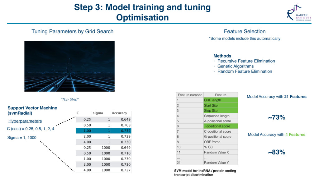
18. Step 3: Model training and tuning Optimisation Tuning Parameters by Grid Search “The Grid” Support Vector Machine (svmRadial) Hyperparameters C (cost) = 0.25, 0.5, 1, 2, 4 Sigma = 1, 1000 C sigma Accuracy 0.25 1 0.649 0.50 1 0.708 1.00 1 0.732 2.00 1 0.729 4.00 1 0.730 0.25 1000 0.649 0.50 1000 0.710 1.00 1000 0.730 2.00 1000 0.730 4.00 1000 0.727 Feature Selection *Some models include this automatically Feature number Feature 1 ORF length 2 Start Site 3 Stop Site 4 Sequence length 5 A-positional score 6 T-positional score 7 C-positional score 8 G-positional score 8 ORF frame 10 % GC 11 Random Value X … … 21 Random Value Y Model Accuracy with 21 Features Model Accuracy with 4 Features ~73% SVM model for lncRNA / protein coding transcript discrimination Methods • Recursive Feature Elimination • Genetic Algorithms • Random Feature Elimination ~83% Feature number Feature 1 ORF length 2 Start Site 3 Stop Site 4 Sequence length 5 A-positional score 6 T-positional score 7 C-positional score 8 G-positional score 8 ORF frame 10 % GC 11 Random Value X … … 21 Random Value Y
19. Step 4: Model evaluation The Confusion Matrix known Pos known Neg predicted Pos predicted Neg TP TN FP FN Confusion matrix known Pos known Neg predicted Pos predicted Neg 50 70 30 50 Confusion matrix Accuracy = (50 + 70) / 200 = 60% Sensitivity = 50 / 50 + 50 = 50% Precision / Positive predictive value = 50 / (50 + 30) = 62.5% Negative predictive value = 70 / (70 + 50) = 58.3% How many are we getting right? How many of our (known) positives are we getting right? Specificity = 70 / (70 + 30) = 70% How many of our (known) negatives are we getting right? How many of our (predicted) positives are we getting right? How many of our (predicted) negatives are we getting right?
20. Step 4: Model evaluation Metrics with class unbalancing known Pos known Neg predicted Pos predicted Neg 90 510 390 10 Confusion matrix A Accuracy = 60% known Pos known Neg predicted Pos predicted Neg 10 590 310 90 Confusion matrix B Accuracy = 60% Sensitivity = 90% Specificity = 57% Sensitivity = 10% Specificity = 66% PPV = 19% PPV = 3% NPV = 98% NPV = 87% F1 = 31% F1 = 5% + 0% - 80% + 9% -16% - 11% - 26%
21. Step 4: Model evaluation Metrics with class unbalancing 0.0 0.5 1.0 0.0 0.5 1.0 1.5 2.0 2.5 density.default(x = prob_b[, 2]) N = 1000 Bandwidth = 0.08334 Density Classifiers can provide “probability” score for a class probability score Class A Class B 0.0 0.4 0.8 0.0 0.2 0.4 0.6 0.8 1.0 ROC curve AUC = 0.92173 FPR Sensitivity 0.2 0.4 0.6 0.8 0.0 0.4 0.8 0.0 0.2 0.4 0.6 0.8 1.0 ROC curve AUC = 0.91608 FPR Sensitivity 0.2 0.4 0.6 0.8 0.0 0.4 0.8 0.0 0.2 0.4 0.6 0.8 1.0 ROC curve AUC = 0.916882 FPR Sensitivity 0.2 0.4 0.6 0.8 500:500 500:1000 500:2000 Accuracy = 80% F1 = 76% Accuracy = 85% F1 = 74% Accuracy = 90% F1 = 71% 314 488 12 186 314 962 38 186 314 1936 64 186 Receiver Operator Curves known Pos known Neg predicted Pos predicted Neg TP TN FP FN Sensitivity = TP/(known Pos) FPR = FP/(known Neg)
22. Step 5: Insight? • Being able to quickly (and accurately) predict a value can be hugely beneficial Genomic Feature Annotation (e.g. splice elements, TF binding sites) Measurement is often reliant on sequencing depth ($$$), and experimental conditions ($$$) Patient phenotypes (e.g. Drug response, Cancer subtype) Prediction >>> Measurement (invasive, unproductive) • Is there some kind of feature that is important for the model to perform? • Is this consistent across models? • What can your model tell you?
23. Black Boxes of Machine Learning Black Box vs Open Box Machine learning models often dismissed on the grounds of lack of interpretability With advanced models, it is difficult to understand how a model is making a prediction Data Results
24. Step 5: Insight? Feature Importance Most models will have built in feature importance Feature probing (LIME: Local Interpretable Model- agnostic Explanations) Modify the inputs slightly from known cases to determine what features are responsible for outputs Test set analysis Leave-one-out model training Importance ORF length 100.00 ORF start site 19.27 T-positional score 6.54 A-positional score 4.87 G-positional score 3.91 % GC 3.70 caret::VarImp(model) What attributes do a True Positive/True Negative have vs. incorrectly classified examples?
25. Deep Learning At its simplest, a Deep Neural Network just has more layers https://hackernoon.com/log-analytics-with-deep-learning-and-machine-learning-20a1891ff70e
26. A Perceptron http://www.asimovinstitute.org/neural-network-zoo/
27. Deep Learning: Size matters! Linear model v. Random Forest v. Deep Learning Number of training examples (millions) Deep Learning can be good with LOTS of data https://github.com/szilard/benchm-ml/tree/master/x1-data-higgs
28. Deep learning: no more feature engineering?? Deep Learning can bypass the need for feature engineering Is this good? Lacks interpretability and enables model building by non-domain experts Deep Learning methods can identify structural features in data, regardless of context DNA sequence? An image is at its most basic, a (very large) series of spatially related numbers Can be encoded by numbers 0001 = A, 0010 = C etc. http://searchbusinessanalytics.techtarget.com/definition/deep-learning https://www.nature.com/news/computer-science-the-learning-machines-1.14481
29. Some Summary Points • Garbage in, Garbage out • Split test, train, validate (and keep them seperate) • Understand what your performance metrics are telling you • Use some form of interpretive techniques to understand your model
30. Some Resources Elements of Statistical Learning (Hastie, Tibshirani & Friedman) : Free PDF https:// web.stanford.edu/~hastie/ElemStatLearn/ Andrew Ng’s Machine Learning Online Course (Coursera) : https:// www.coursera.org/learn/machine- learning# Deep Learning Courses (also Andrew Ng) : https://www.coursera.org/specializations/ deep-learning Read / Watch (and do) Do R: caret (Classification And REgression Training) http://topepo.github.io/caret/index.html python: scikit learn http://scikit-learn.org/stable/