Causal Inference 2022 Week 4

Transcript

1. CAUSAL INFERENCE Adjustment William Lowe Hertie School Data Science Lab 2022-02-28
2. REGRESSION BASICS 1 A regression function: E[log wage education] A regression function approximated logwage = β + (education)βe + є
3. REGRESSION BASICS 2 C ... Non-linear transformations like log can create or remove linearity E[log wage education] ≠ logE[wage education]
4. REGRESSION BASICS 2 C ... Non-linear transformations like log can create or remove linearity E[log wage education] ≠ logE[wage education] M When you think wages are multipliers wage = γ γ(education) e you think that logwage = β + (education)βe In case you ever wondered why there were logs everywhere...
5. REGRESSION BASICS 3 A regression function need not be linear In this data, LD for pedestrians is about mph ( kph) Probably a little lower now B When the outcome is binary, e.g. deathi = if pedestrian i died and otherwise E[death speed] = P(death speed) which is also a population proportion
6. REGRESSION BASICS 3 A regression function need not be linear In this data, LD for pedestrians is about mph ( kph) Probably a little lower now B When the outcome is binary, e.g. deathi = if pedestrian i died and otherwise E[death speed] = P(death speed) which is also a population proportion For mph this is the limit as N → ∞ of ∑N i I[speedi = ]deathi ∑N i I[speedi = ]
7. REGRESSION MODELS AS PREDICTION 4 Predict post.score S from pre.score P and grade G єP P G S єS єG
8. REGRESSION MODELS AS PREDICTION 4 Predict post.score S from pre.score P and grade G єP P G S єS єG L S = β + Gβд + Pβp + єS Parameters: → [β , βд, βp, Var(єS )] Find values for these that make a data set most likely
9. REGRESSION MODELS AS PREDICTION 4 Predict post.score S from pre.score P and grade G єP P G S єS єG L S = β + Gβд + Pβp + єS Parameters: → [β , βд, βp, Var(єS )] Find values for these that make a data set most likely e best value for two parameters...
10. REGRESSION MODELS AS PREDICTION 5 єP P G S єS єG is is a model of P(S G, P) from which we can make predictions
11. REGRESSION MODELS AS PREDICTION 5 єP P G S єS єG is is a model of P(S G, P) from which we can make predictions e best∗ choice is E[S G, P] = β + Gβд + Pβp * in a mean squared error sense
12. REGRESSION MODELS AS PREDICTION 5 єP P G S єS єG is is a model of P(S G, P) from which we can make predictions e best∗ choice is E[S G, P] = β + Gβд + Pβp * in a mean squared error sense R In a model with an intercept, residuals S − E[S G, P] are mean and orthogonal to the predictions
13. REGRESSION MODELS AS PREDICTION 5 єP P G S єS єG is is a model of P(S G, P) from which we can make predictions e best∗ choice is E[S G, P] = β + Gβд + Pβp * in a mean squared error sense R In a model with an intercept, residuals S − E[S G, P] are mean and orthogonal to the predictions M We can always divide Si into → µi a function of observed variables → ei an orthogonal residual such that Si = µi + ei Whether e tracks єS is a di erent question...
14. ...AND AS ADJUSTMENT FOR CONFOUNDING 6 e e ect of pre.score P on post.score S is confounded by grade G єP P G S єS єG F ere is a relationship of interest P → S G just confounds it.
15. ...AND AS ADJUSTMENT FOR CONFOUNDING 6 e e ect of pre.score P on post.score S is confounded by grade G єP P G S єS єG F ere is a relationship of interest P → S G just confounds it. A Frisch and Waugh showed in (and Lovell ( ) generalized) an important fact about linear regression models (Lovell, , for a short proof).
16. ...AND AS ADJUSTMENT FOR CONFOUNDING 6 e e ect of pre.score P on post.score S is confounded by grade G єP P G S єS єG F ere is a relationship of interest P → S G just confounds it. A Frisch and Waugh showed in (and Lovell ( ) generalized) an important fact about linear regression models (Lovell, , for a short proof). Consider three linear models S = β + Gβд + Pβp + є S = β(S) + Gβ(S) д + є (S model) P = β(P) + Gβ(P) д + є (P model)
17. ...AND AS ADJUSTMENT FOR CONFOUNDING 6 e e ect of pre.score P on post.score S is confounded by grade G єP P G S єS єG F ere is a relationship of interest P → S G just confounds it. A Frisch and Waugh showed in (and Lovell ( ) generalized) an important fact about linear regression models (Lovell, , for a short proof). Consider three linear models S = β + Gβд + Pβp + є S = β(S) + Gβ(S) д + є (S model) P = β(P) + Gβ(P) д + є (P model) so that E[S G] = β(S) + Gβ(S) д E[P G] = β(P) + Gβ(P) д
18. ISOLATING USEFUL VARIATION 7 єP P G S єS єG Construct the residuals from each sub-model r(S) = S − E[S G] r(P) = P − E[P G]
19. ISOLATING USEFUL VARIATION 7 єP P G S єS єG Construct the residuals from each sub-model r(S) = S − E[S G] r(P) = P − E[P G] and t the following linear model∗ r(S) = r(P)β(FWL) + є * residuals are mean , so no intercept is required T (Frisch Waugh Lovell): When the original model is S = β + Gβд + Pβp + є then β(FWL) = βp
20. ISOLATING USEFUL VARIATION 7 єP P G S єS єG Construct the residuals from each sub-model r(S) = S − E[S G] r(P) = P − E[P G] and t the following linear model∗ r(S) = r(P)β(FWL) + є * residuals are mean , so no intercept is required T (Frisch Waugh Lovell): When the original model is S = β + Gβд + Pβp + є then β(FWL) = βp W ? → r(P) = P − E[P G] tracks єP → r(S) = S − E[S G] tracks єS Association between these is due to P →S
21. THE FRISCH, THE WAUGH AND THE LOVELL 8
22. COMPARED TO STRATIFICATION 9 S → Divide up the data by grade → Measure the relationship between P and S in each data set → Average the estimates In each subset, there is no variation in G
23. COMPARED TO STRATIFICATION 9 S → Divide up the data by grade → Measure the relationship between P and S in each data set → Average the estimates In each subset, there is no variation in G R Add dummy variables like grade2 → Coe cients on grade dummies capture all the variation G can cause in S → A er adjusting for that, what remains has no variation due to G
24. FIXED EFFECTS 10 U Substantively, the coe cient on grade2 represents whatever it is about being in grade that a ects S → Shared by every class in the same grade → Constant for those classes
25. FIXED EFFECTS 10 U Substantively, the coe cient on grade2 represents whatever it is about being in grade that a ects S → Shared by every class in the same grade → Constant for those classes F How to remove that variation? → Include a set of dummy variables like grade2 → Adjust the other variables (the FWL strategy) Confusingly, these are both referred to as adding ‘ xed e ects’
26. FIXED EFFECTS 10 U Substantively, the coe cient on grade2 represents whatever it is about being in grade that a ects S → Shared by every class in the same grade → Constant for those classes F How to remove that variation? → Include a set of dummy variables like grade2 → Adjust the other variables (the FWL strategy) Confusingly, these are both referred to as adding ‘ xed e ects’ C Most o en you will encounter → unit: country, city, person → time: year, month, cohort M → ‘one way’: only unit, or only time → ‘two way’: both
27. FIXED EFFECTS 10 U Substantively, the coe cient on grade2 represents whatever it is about being in grade that a ects S → Shared by every class in the same grade → Constant for those classes F How to remove that variation? → Include a set of dummy variables like grade2 → Adjust the other variables (the FWL strategy) Confusingly, these are both referred to as adding ‘ xed e ects’ C Most o en you will encounter → unit: country, city, person → time: year, month, cohort M → ‘one way’: only unit, or only time → ‘two way’: both A Fixed e ects remove all the unmeasured but group-speci c confounding factors → Better hope there’s something le ...
28. ASIDE: MULTILEVEL MODELS 11 Sometimes that group level variation is pretty interesting!
29. ASIDE: MULTILEVEL MODELS 11 Sometimes that group level variation is pretty interesting!
30. HOW DOES DEMOCRACY AFFECT FDI? 12 -2.5 0.0 2.5 5.0 7.5 FDI From Jensen ( )
31. FOREIGN DIRECT INVESTMENT 13 Does being more democratic lead to more FDI? According to Jensen ( ), yes. We’ll look at a (simpli ed) version of his time series cross-sectional analysis → Worldwide (but with some missingness) → years of annual data: - → Regime on a point scale (higher, more democratic) → Controls for lots of potential confounders, predictors of FDI, and country xed e ects → small but signi cant positive e ect of regime time on FDI
32. FOREIGN DIRECT INVESTMENT 13 Does being more democratic lead to more FDI? According to Jensen ( ), yes. We’ll look at a (simpli ed) version of his time series cross-sectional analysis → Worldwide (but with some missingness) → years of annual data: - → Regime on a point scale (higher, more democratic) → Controls for lots of potential confounders, predictors of FDI, and country xed e ects → small but signi cant positive e ect of regime time on FDI Regime type / democracy score is continuous, so we’ll think of the causal e ect of regime type as → the di erence in expected FDI for an exogenous one unit increase in democracy
33. FOREIGN DIRECT INVESTMENT 13 Does being more democratic lead to more FDI? According to Jensen ( ), yes. We’ll look at a (simpli ed) version of his time series cross-sectional analysis → Worldwide (but with some missingness) → years of annual data: - → Regime on a point scale (higher, more democratic) → Controls for lots of potential confounders, predictors of FDI, and country xed e ects → small but signi cant positive e ect of regime time on FDI Regime type / democracy score is continuous, so we’ll think of the causal e ect of regime type as → the di erence in expected FDI for an exogenous one unit increase in democracy S → e e ect of regime may not be the same everywhere → We may not know how it varies Can we estimate an ATE when there are heterogenous treatment e ects?
34. BEST CASE SCENARIO 14 єD D G F єF єG e e ect of democracy D on foreign direct investment F with geopolitical controls G
35. BEST CASE SCENARIO 14 єD D G F єF єG e e ect of democracy D on foreign direct investment F with geopolitical controls G Can we estimate the e ect of D on F using regression? → If the e ect is constant: de nitely
36. BEST CASE SCENARIO 14 єD D G F єF єG e e ect of democracy D on foreign direct investment F with geopolitical controls G Can we estimate the e ect of D on F using regression? → If the e ect is constant: de nitely H Consider heterogenous additive e ects τi such that Fi = Fi + τi Di (F , τ) ⊥ ⊥ D G
37. BEST CASE SCENARIO 14 єD D G F єF єG e e ect of democracy D on foreign direct investment F with geopolitical controls G Can we estimate the e ect of D on F using regression? → If the e ect is constant: de nitely H Consider heterogenous additive e ects τi such that Fi = Fi + τi Di (F , τ) ⊥ ⊥ D G ATE e average treatment e ect is by de nition ATE = E[τ] Ideally, our regression coe cient βD identi es this... → Sometimes not...
38. HETEROGENOUS TREATMENT EFFECTS 15 єD D G F єF єG W ? Back in FWL we considered the residuals from model of D given G ri (D) = Di − E[D Gi ] De ne a weight that is the square of this wi = ri (D)
39. HETEROGENOUS TREATMENT EFFECTS 15 єD D G F єF єG W ? Back in FWL we considered the residuals from model of D given G ri (D) = Di − E[D Gi ] De ne a weight that is the square of this wi = ri (D) E[w] is the variance of democracy prediction errors using geo-political variables → w is large when D is unpredictable from G
40. HETEROGENOUS TREATMENT EFFECTS 15 єD D G F єF єG W ? Back in FWL we considered the residuals from model of D given G ri (D) = Di − E[D Gi ] De ne a weight that is the square of this wi = ri (D) E[w] is the variance of democracy prediction errors using geo-political variables → w is large when D is unpredictable from G C Why do we care?
41. HETEROGENOUS TREATMENT EFFECTS 15 єD D G F єF єG W ? Back in FWL we considered the residuals from model of D given G ri (D) = Di − E[D Gi ] De ne a weight that is the square of this wi = ri (D) E[w] is the variance of democracy prediction errors using geo-political variables → w is large when D is unpredictable from G C Why do we care? Because (Aronow & Samii, ) βD = E[wi τi ] E[wi ]
42. NOMINAL COUNTRY WEIGHTS 16
43. HIGHER COUNTRY WEIGHTS 17 0.01 0.02 0.03 0.04 0.05 0.06 OLS weights
44. LOWER COUNTRY WEIGHTS 18 0.001 0.002 0.003 0.004 0.005 0.006 OLS weights
45. LOWEST WEIGHTED COUNTRIES 19 Haiti Honduras Russian Federation South Africa Yemen, Rep. Albania Benin Central African Republic Congo, Rep. Germany 1980 1990 1980 1990 1980 1990 1980 1990 1980 1990 -6 -4 -2 0 2 -6 -4 -2 0 2 year Fvar5 5 10 15 regime
46. HIGHEST WEIGHTED COUNTRIES 20 Peru Philippines Poland Uruguay Zimbabwe Argentina Hungary Madagascar Niger Pakistan 1980 1990 1980 1990 1980 1990 1980 1990 1980 1990 0.0 2.5 5.0 7.5 10.0 0.0 2.5 5.0 7.5 10.0 year Fvar5 5 10 15 regime
47. WEIGHTING 21 H Countries with → that have plenty of observations → large variations in democracy levels and FDI → that is hard to predict from country xed e ects and other controls L Countries with → that have few observations → constant / nearly constant democracy and FDI → democracy levels predictable from xed e ects and other controls G No variation, so zero weight → As far as regression can tell, there is no possibility of regime change in Germany (because there’s none in the data) → Assumption: positivity fails / the counterfactual does not exist More detailed comparison in ch. . of Angrist and Pischke ( ) and a slightly more general framework in Hirano et al. ( )
48. WHEN IS THIS A PROBLEM? 22 C Not when e ects are constant τi = τ R Not in randomized experiments β = E[wi τi ] E[wi ] = E[wi ]E[τi ] E[wi ] = E[τi ] O Maybe here. Some cases will matter a lot more than others
49. MODESTY ABOUT REGRESSION 23 It feels like regression on representative samples ought to get us externally valid results... → Alas, not necessarily Estimates from a randomized experiment are only directly informative for the subpopulation whose treatment status can be manipulated by the investigator. Estimates from an observational study can only be directly informative for the subpopulation that exhibits some unpredictability in their treatment status a er accounting for control variables. (Aronow & Samii, )
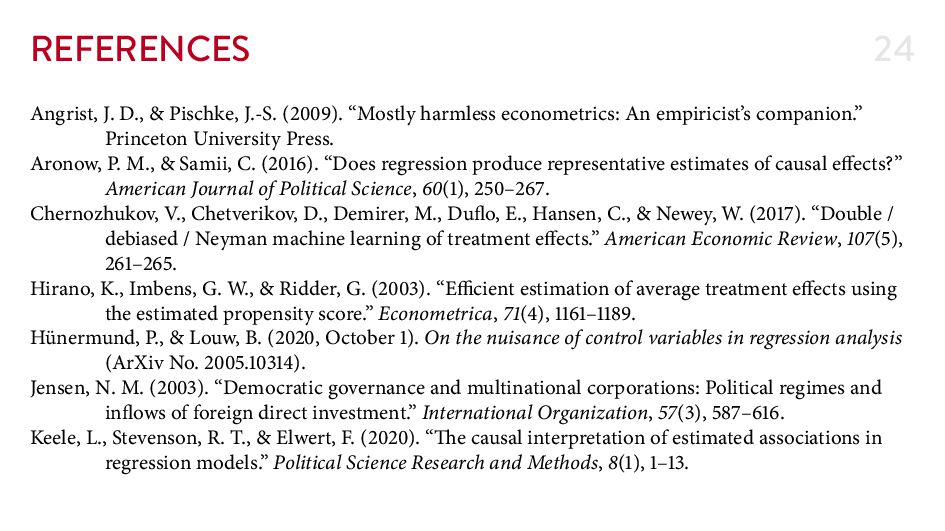
50. REFERENCES 24 Angrist, J. D., & Pischke, J.-S. ( ). “Mostly harmless econometrics: An empiricist’s companion.” Princeton University Press. Aronow, P. M., & Samii, C. ( ). “Does regression produce representative estimates of causal e ects?” American Journal of Political Science, ( ), – . Chernozhukov, V., Chetverikov, D., Demirer, M., Du o, E., Hansen, C., & Newey, W. ( ). “Double / debiased / Neyman machine learning of treatment e ects.” American Economic Review, ( ), – . Hirano, K., Imbens, G. W., & Ridder, G. ( ). “E cient estimation of average treatment e ects using the estimated propensity score.” Econometrica, ( ), – . Hünermund, P., & Louw, B. ( , October ). On the nuisance of control variables in regression analysis (ArXiv No. . ). Jensen, N. M. ( ). “Democratic governance and multinational corporations: Political regimes and in ows of foreign direct investment.” International Organization, ( ), – . Keele, L., Stevenson, R. T., & Elwert, F. ( ). “ e causal interpretation of estimated associations in regression models.” Political Science Research and Methods, ( ), – .
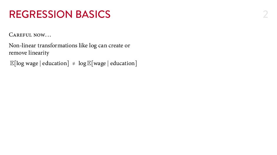
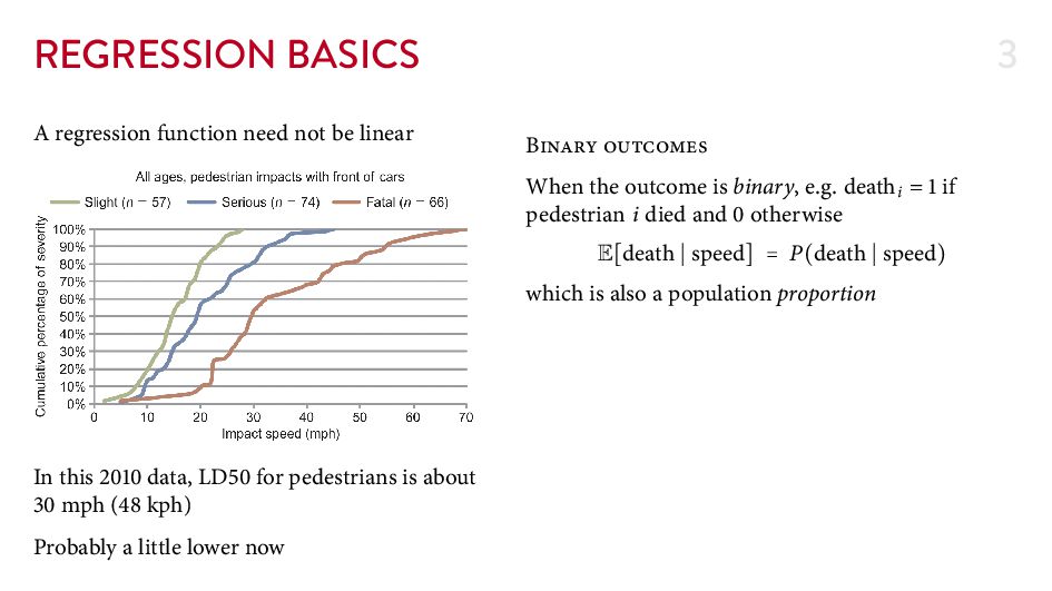
51. REFERENCES 25 Lovell, M. C. ( ). “Seasonal adjustment of economic time series and multiple regression analysis.” Journal of the American Statistical Association, ( ), – . Lovell, M. C. ( ). “A simple proof of the FWL theorem.” e Journal of Economic Education, ( ), – .