Data Science and Decisions 2022: Week 6

Transcript

1. DATA SCIENCE AND DECISION MAKING Decision making in and by groups William Lowe Hertie School Data Science Lab 2022-04-20
2. PLAN 1 Why combine judgments? e view from data science Bias, variance, and error Groupthink and other bad outcomes Multiverse models in science Motivating multiverses with Bayes e limits of model averaging Deliberation and social choice
3. WHY COMBINE? 2 Assume M models (or any decision makers) each of whom predicts a target Y as ˆ Ym = Y + єm and compare this to a committee prediction ˆ Y Com = M M m ˆ Ym
4. WHY COMBINE? 2 Assume M models (or any decision makers) each of whom predicts a target Y as ˆ Ym = Y + єm and compare this to a committee prediction ˆ Y Com = M M m ˆ Ym S Model m has mean squared error (MSE) Em = E[( ˆ Ym − Y) ] = E[єm] e average MSE error of M such models is E Av = M M m Em = M M m E[єm]
5. WHY COMBINE? 2 Assume M models (or any decision makers) each of whom predicts a target Y as ˆ Ym = Y + єm and compare this to a committee prediction ˆ Y Com = M M m ˆ Ym S Model m has mean squared error (MSE) Em = E[( ˆ Ym − Y) ] = E[єm] e average MSE error of M such models is E Av = M M m Em = M M m E[єm] C E Com = E ⎡ ⎢ ⎢ ⎢ ⎢ ⎣ ⎛ ⎝ M M m ˆ Ym ˆ YCom −Y ⎞ ⎠ ⎤ ⎥ ⎥ ⎥ ⎥ ⎦ = E ⎡ ⎢ ⎢ ⎢ ⎢ ⎣ M M m єm ⎤ ⎥ ⎥ ⎥ ⎥ ⎦ If model errors are E[єm] = (well-speci ed) E[єmєm′ ] = m ≠ m′ (uncorrelated) then E Com = M M m E[є ] = M EAv
6. WHY COMBINE? 2 Assume M models (or any decision makers) each of whom predicts a target Y as ˆ Ym = Y + єm and compare this to a committee prediction ˆ Y Com = M M m ˆ Ym S Model m has mean squared error (MSE) Em = E[( ˆ Ym − Y) ] = E[єm] e average MSE error of M such models is E Av = M M m Em = M M m E[єm] C E Com = E ⎡ ⎢ ⎢ ⎢ ⎢ ⎣ ⎛ ⎝ M M m ˆ Ym ˆ YCom −Y ⎞ ⎠ ⎤ ⎥ ⎥ ⎥ ⎥ ⎦ = E ⎡ ⎢ ⎢ ⎢ ⎢ ⎣ M M m єm ⎤ ⎥ ⎥ ⎥ ⎥ ⎦ If model errors are E[єm] = (well-speci ed) E[єmєm′ ] = m ≠ m′ (uncorrelated) then E Com = M M m E[є ] = M EAv Simply averaging gives us M times less error!
7. WHY COMBINE 3 C Any model committee is another model E
8. WHY COMBINE 3 C Any model committee is another model E Model combination as a model design strategy is known as ensemble learning Important examples → Bagging (‘bootstrap aggregating’ Breiman, ) → Boosting (Freund & Schapire, ) Hint: When someone suggests Deep Learning, try XGBoost rst!
9. WHY COMBINE 3 C Any model committee is another model E Model combination as a model design strategy is known as ensemble learning Important examples → Bagging (‘bootstrap aggregating’ Breiman, ) → Boosting (Freund & Schapire, ) Hint: When someone suggests Deep Learning, try XGBoost rst! W ? Model combination helps navigates the bias-variance decomposition → Individual models can a ord to be less biased and quite variable → because averaging reduces committee variance → e complete model has at least as little bias as its components Let’s brie y review the bias-variance tradeo ...
10. BIAS, VARIANCE, AND ERROR 4 −2 −1 0 1 2 0.00 0.25 0.50 0.75 1.00 Degree 0 1 2 3 6 8 MSE = variance + bias + noise → Model : no error, high variance, low bias → Model : high error, low variance, high bias → Model : lowest error, mid variance, mid bias 0.00 0.25 0.50 0.75 0 1 2 3 4 5 6 7 8 9 Degree RMSE Sample in out In-sample error is a good guide to out of sample performance...until it isn’t → is is the bias-variance tradeo
11. WHY IT WORKS 5 eoretically, we can guarantee that E Com ≤ EAv Whether we get M times less error depends on our A → Correct model speci cations, e.g. no missing variables / unconfounded → Uncorrelated errors, e.g. errors independent in time and group What if these are not true? → Build a better model! → Learn the model error correlation matrix and make a weighted average Perfectly correlated judgment errors too
12. IN PEOPLE 6 H ? Risk factors for groupthink (according to Janis): → Group cohesiveness (correlated errors) → Group insulation (model mispeci cation) → Leadership style (weighting, correlated errors) → Methodical information processing procedures S Increase committee diversity, e.g. board composition
13. IN PEOPLE 6 H ? Risk factors for groupthink (according to Janis): → Group cohesiveness (correlated errors) → Group insulation (model mispeci cation) → Leadership style (weighting, correlated errors) → Methodical information processing procedures S Increase committee diversity, e.g. board composition O en thought to work because of → increased representation → new perspectives From our perspective, maybe because increased diversity → decorrelates errors → makes for better speci ed models (participants) Note: → ‘playing devil’s advocate’ (or WWJD?) fakes actual diversity by anti-correlating errors
14. ENSEMBLES IN RESEARCH 7 ere are usually lots of di erent ways to study the same question Inter-researcher disagreement is o en driven by di erent → subsets of data, coding strategies → DV, IV, control choices → variable transformations, e.g. logs and cut-points → statistical assumptions, e.g. xed vs random e ects, interactions, and non-linearities
15. ENSEMBLES IN RESEARCH 7 ere are usually lots of di erent ways to study the same question Inter-researcher disagreement is o en driven by di erent → subsets of data, coding strategies → DV, IV, control choices → variable transformations, e.g. logs and cut-points → statistical assumptions, e.g. xed vs random e ects, interactions, and non-linearities Identify models with decision makers How to make a nal inference? → Refuse! → Choose the best: model selection → Combine them: model averaging Multiverse analysis (Steegen et al., )
16. ENTER THE MULTIVERSE 8 (Schweinsberg et al., )
17. ENTER THE MULTIVERSE 9 I point estimates are above zero and are below → Did they con rm hypothesis ? → Is the probability of hypothesis / ? How to combine these estimates?
18. BAYES AGAIN 10 Consider a prior over models M a.k.a. preprocessing choices, of data D where Z is our z-score. M By the Law of Total Probability P(Z D) = M m P(Z, M = m D) = M m P(Z M = m, D)P(M = m D) P(M = m D) is sometimes called a ‘Bayes Factor’
19. BAYES AGAIN 10 Consider a prior over models M a.k.a. preprocessing choices, of data D where Z is our z-score. M By the Law of Total Probability P(Z D) = M m P(Z, M = m D) = M m P(Z M = m, D)P(M = m D) P(M = m D) is sometimes called a ‘Bayes Factor’ If we don’t both to distinguish between how likely each model is in the light of the data then, maybe... P(M = m D) = P(M = m) = M (a ‘ at’ prior) What if we wanted to do things properly? Consider a model with parameters β Bayesian inferences about β should be based on P(β D, M = m) which is... P(D β, M = m)P(β M = m) P(D M = m) e marginal likelihood of the data is the denominator → How likely each M makes the data, averaging out uncertainty about β from which comes the Bayes Factor P(M = m D) = P(D M = m) P(M = m) P(D)
20. BAYES AGAIN 11 It’s fairly implausible that P(M = m D) = P(M = m) = M (though not impossible) → If some model speci cations are a priori more likely than others P(M = m) ≠ M → If model speci cation choices are independent of D, i.e. you don’t learn anything about them by seeing the data P(M = m D) ≠ P(M = m)
21. BAYES AGAIN 11 It’s fairly implausible that P(M = m D) = P(M = m) = M (though not impossible) → If some model speci cations are a priori more likely than others P(M = m) ≠ M → If model speci cation choices are independent of D, i.e. you don’t learn anything about them by seeing the data P(M = m D) ≠ P(M = m) M We can also use it to select a single model (but why?)
22. BAYES AGAIN 11 It’s fairly implausible that P(M = m D) = P(M = m) = M (though not impossible) → If some model speci cations are a priori more likely than others P(M = m) ≠ M → If model speci cation choices are independent of D, i.e. you don’t learn anything about them by seeing the data P(M = m D) ≠ P(M = m) M We can also use it to select a single model (but why?) O ’ R → in exible model: few Ds but more likely → exible model: many Ds less likely Flexibility and data t trade o (Bishop, )
23. IN PEOPLE 12 H ? Decision weighting should re ect expertise on this kind of data: P(M = m D) for my D → Small numbers of experts (but not one) → Not large numbers of uninformed Tetlock and Gardner ( ) o ers two cognitive styles → Hedgehogs (assign high probability to relatively few data sets) → Foxes (assign lower probability to a wider range) We should probably think of these as a continuum
24. THE LIMITS OF AVERAGING 13 Some things don’t make sense to average D → R: rainfall → Y: crop yields → P: political con ict → F: famine Question: → What is the e ect of political con ict on famine? What variables to choose? (List, )
25. THE LIMITS OF AVERAGING 13 Some things don’t make sense to average D → R: rainfall → Y: crop yields → P: political con ict → F: famine Question: → What is the e ect of political con ict on famine? What variables to choose? (List, ) In a model of F → Expert would condition on Y → Expert would not condition on Y → Expert would only condition on Y if they wanted the ‘direct e ect’ of P
26. THE LIMITS OF AVERAGING 14 D
27. THE LIMITS OF AVERAGING 14 D C Our experts can t their models and we can average the predictions → Predictively this might be ne? → e marginal e ect of P on F is a mixture of very di erent ‘worlds’ We will be working with Expert ’s model (it’s a superset of the other two) But there’s no guarantee that the superset of more experts will make any sense (or even be acyclic!)
28. HOW (NOT) TO AGGREGATE DAGS 15
29. GETTING ON THE SAME PAGE 16 Christopher Gandrud, earlier in the course
30. REVISITING PAPAL CHOICE 17 S eorems from Arrow (Arrow, ), Gibbard and Satterthwaite (Gibbard, ; Satterthwaite, ) suggest → Intuitive criteria for ‘voting’ cannot be simultaneously satis ed T [with deliberation] there would not be any need for an aggregating mechanism, since a rational discussion would tend to produce unanimous preferences Jon Elster, in Matravers and Pike ( ) Deliberation increases single peakedness, a.k.a. meta-agreement (Dryzek & List, ) Subsequent voting will be immune to Arrow-like problems
31. IDEOLOGY AND SOPHISTICATION 18 Broockman ( ) points out that sophisticated respondents have low-D preferences → eir views on di erent policies are not independent → Equivalently, their e ective D is lower than the number of questions you ask them S Unsophisticated voters have nearly independent preferences → Many preference inference methods assume sophistication, e.g. averages of directed responses, scaling models, etc. → ese will put sophisticated voters in the right place, and unsophisticated voters in the middle anyway despite them being mostly elsewhere Ideology is a regularizer / dimensionality reducer / preference structurer... Deliberation increases sophistication!
32. PLAN 19 Why combine judgments? Bias, variance, and error Groupthink and other bad outcomes Multiverse models in science Motivating multiverses with Bayes e limits of model averaging Deliberation and social choice
33. REFERENCES 20 Arrow, K. J. ( ). Social choice and individual values. John Wiley & Sons. Bishop, C. M. ( ). Neural networks for pattern recognition. Oxford University Press. Breiman, L. ( ). Bagging predictors. Machine Learning, ( ), – . Broockman, D. E. ( ). Approaches to studying policy representation. Legislative Studies Quarterly, ( ), – . Dryzek, J. S., & List, C. ( ). Social choice theory and deliberative democracy: A reconciliation. British Journal of Political Science, ( ), – . Freund, Y., & Schapire, R. E. ( ). A decision-theoretic generalization of on-line learning and an application to boosting. Journal of Computer and System Sciences, ( ), – . Gibbard, A. ( ). Manipulation of voting schemes: A general result. Econometrica, ( ), . Hornik, K., Stinchcombe, M., & White, H. ( ). Multilayer feedforward networks are universal approximators. Neural Networks, , – . List, C. ( ). e theory of judgment aggregation: An introductory review. Synthese, ( ), – . Matravers, D., & Pike, J. ( ). Debates in contemporary political philosophy: An anthology. Routledge.
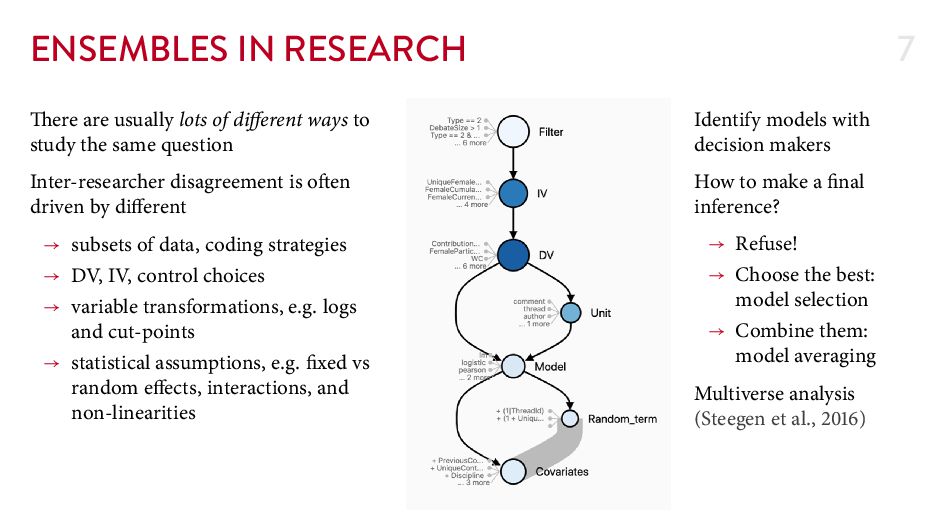
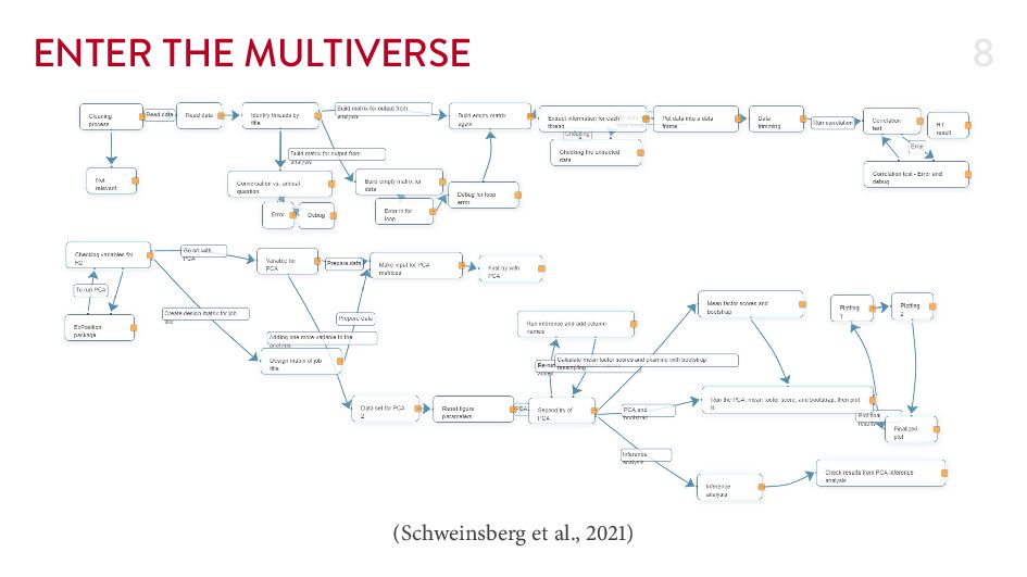
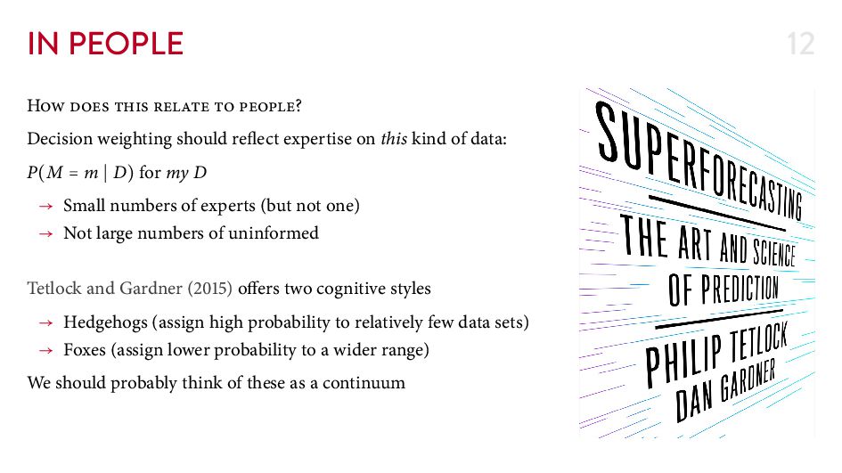
34. REFERENCES 21 Rumelhart, D. E. (Ed.). ( ). Parallel distributed processing. : Foundations. MIT Press. Satterthwaite, M. A. ( ). Strategy-proofness and Arrow’s conditions: Existence and correspondence theorems for voting procedures and social welfare functions. Journal of Economic eory, ( ), – . Schweinsberg, M., Feldman, M., Staub, N., van den Akker, O. R., van Aert, R. C. M., van Assen, M. A. L. M., Liu, Y., Altho , T., Heer, J., Kale, A., Mohamed, Z., Amireh, H., Venkatesh Prasad, V., Bernstein, A., Robinson, E., Snellman, K., Amy Sommer, S., Otner, S. M. G., Robinson, D., ... Luis Uhlmann, E. ( ). Same data, di erent conclusions: Radical dispersion in empirical results when independent analysts operationalize and test the same hypothesis. Organizational Behavior and Human Decision Processes, , – . Steegen, S., Tuerlinckx, F., Gelman, A., & Vanpaemel, W. ( ). Increasing transparency through a multiverse analysis. Perspectives on Psychological Science, ( ), – . Tetlock, P. E., & Gardner, D. ( ). Superforecasting: e art and science of prediction. Crown Publishers.
35. CRAZY FLEXIBLE MODELS 22 A old school multilayer perceptron (MLP, Rumelhart, ) with one hidden layer: A universal approximator, due to the internal non-linearity (Hornik et al., ) A linear combination of J models E[Y X . . . XD] = J j βjϕj(X . . . XD) where ϕj is a non-linear function of a linear combination of inoput data ϕj(X . . . XD) = ( + exp(− d βjd Xd )) at’s → a model with D × J + J parameters → A regression on the output of J logistic regressions on the input data