and Andrew Zisserman // Microsoft Research Sponsored 1 IEEE Transactions on Pattern Analysis and Machine Intelligence, Vol. 33, No. 4, April 2011 Shao-Chung Chen Presentation on “Machine Learning”, June 18 2013
engines provides an effortless route • poor precision (32% for 1, avg. 39%; w/ Google) • restricted # of downloads (1000 w/ Google) • automatically harvest image databases • from the web • with help of search engines 2
engines provides an effortless route • poor precision (32% for 1, avg. 39%; w/ Google) • restricted # of downloads (1000 w/ Google) • automatically harvest image databases • from the web • with help of search engines • precision above 55% on average 2
probabilistic Latent Semantic Analysis (pLSA) • Hierarchical Dirichlet Process • + text on the original page (with image search) • above approaches • poor precision • restricted by the # of downloads 3
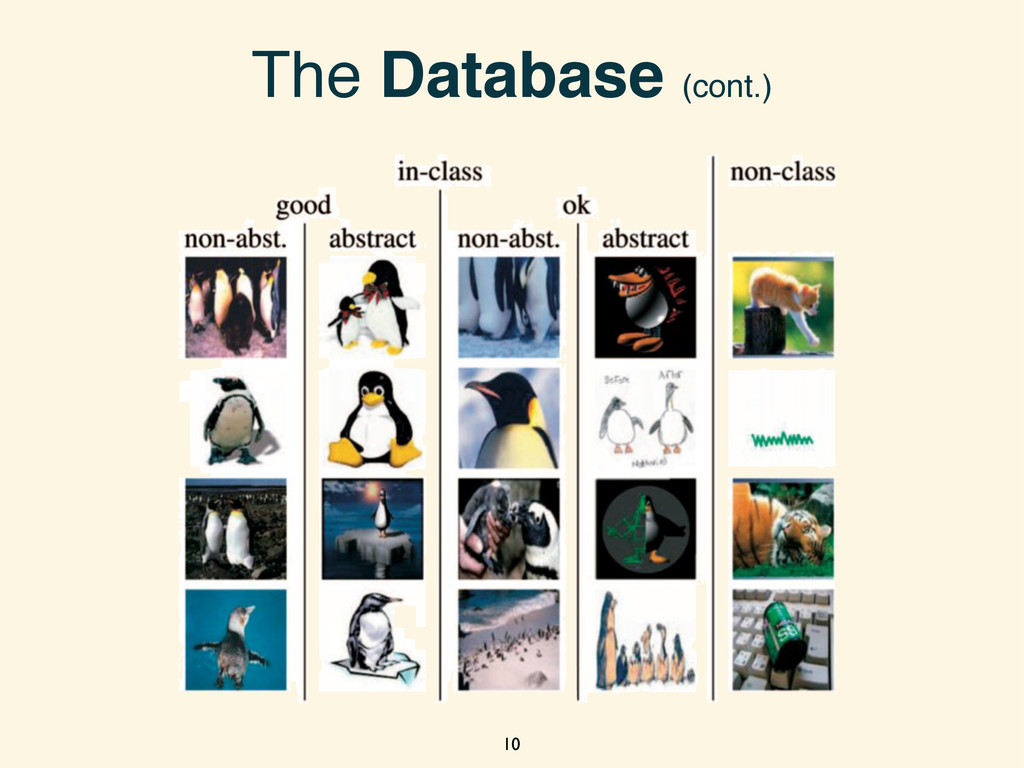
eliminate the download restriction • phase #1 • topics — based on the words on the pages • using Latent Dirichlet Allocation on text • images — near by the text — top ranked 4
eliminate the download restriction • phase #1 • topics — based on the words on the pages • using Latent Dirichlet Allocation on text • images — near by the text — top ranked • labeling — positive/negative image clusters 4
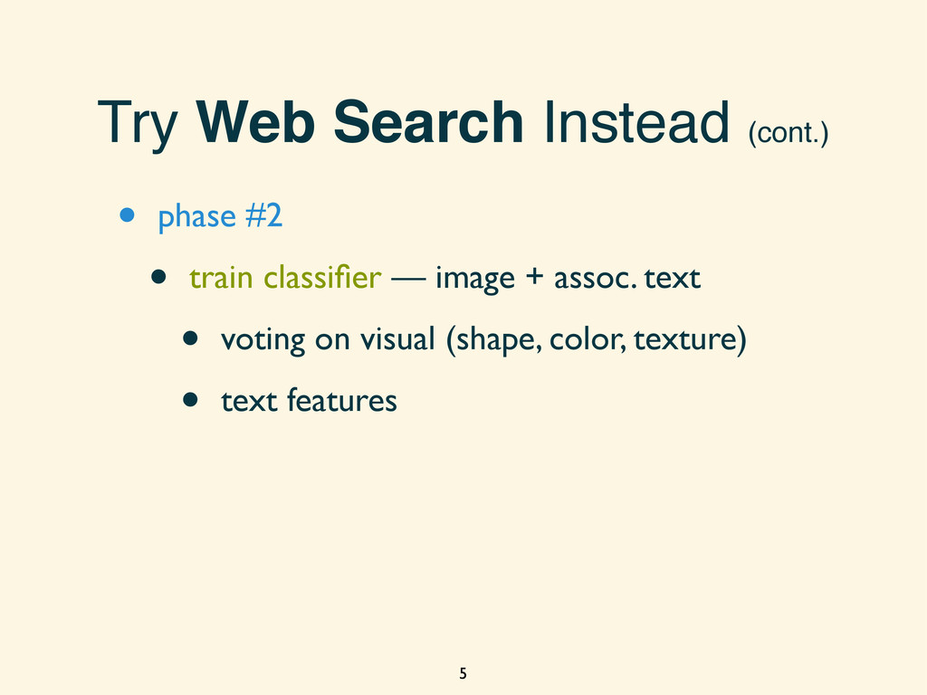
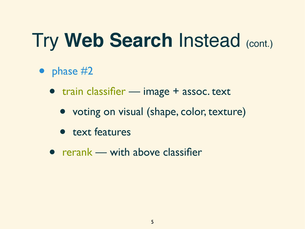
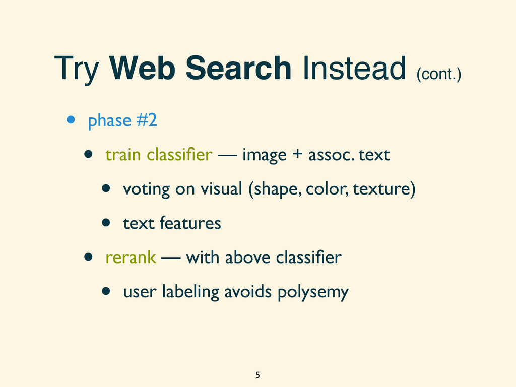
classifier — image + assoc. text • voting on visual (shape, color, texture) • text features • rerank — with above classifier • user labeling avoids polysemy 5
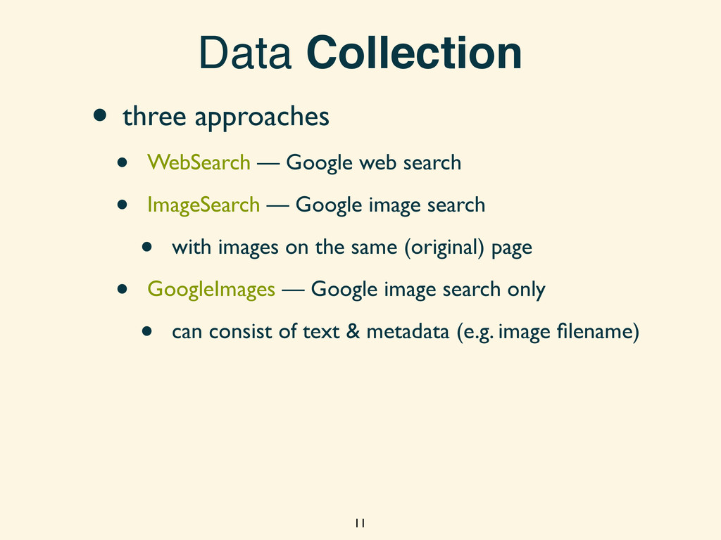
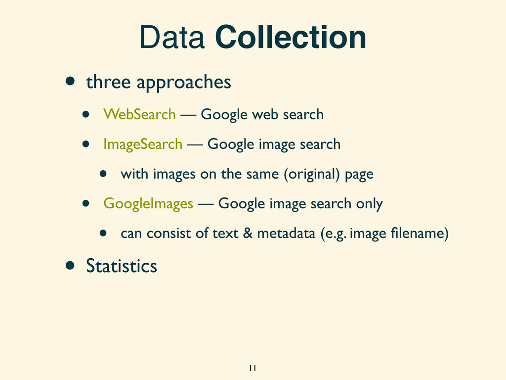
search • ImageSearch — Google image search • with images on the same (original) page • GoogleImages — Google image search only • can consist of text & metadata (e.g. image filename) 11
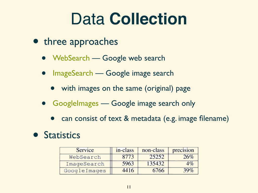
search • ImageSearch — Google image search • with images on the same (original) page • GoogleImages — Google image search only • can consist of text & metadata (e.g. image filename) • Statistics 11
search • ImageSearch — Google image search • with images on the same (original) page • GoogleImages — Google image search only • can consist of text & metadata (e.g. image filename) • Statistics 11
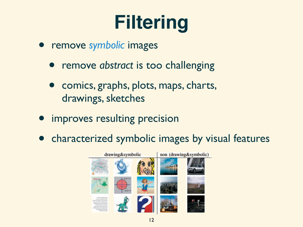
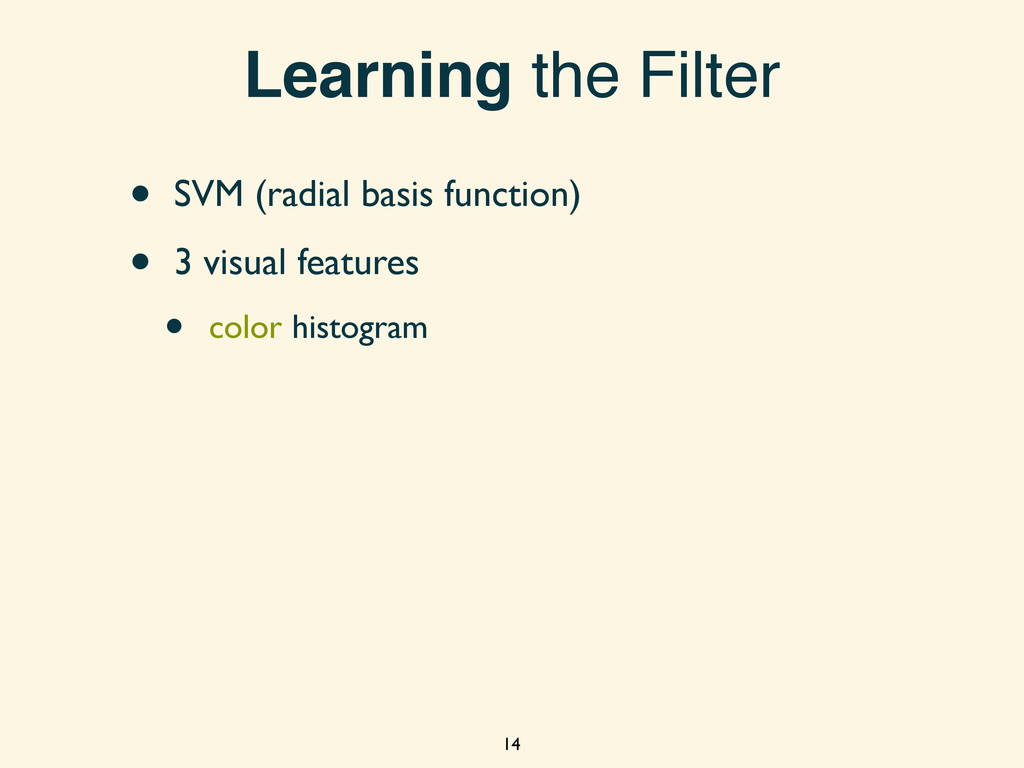
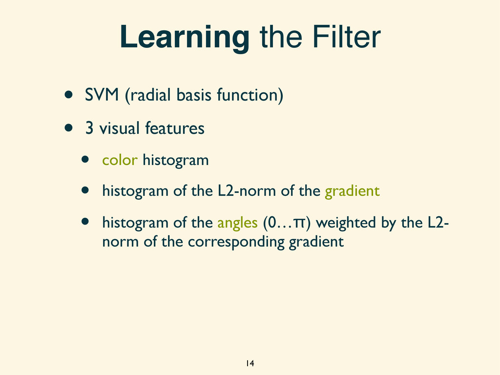
visual features • color histogram • histogram of the L2-norm of the gradient • histogram of the angles (0…π) weighted by the L2- norm of the corresponding gradient 14
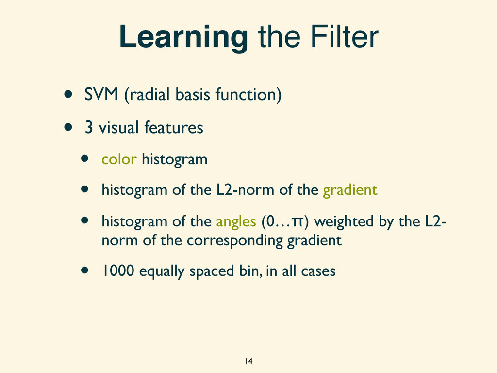
visual features • color histogram • histogram of the L2-norm of the gradient • histogram of the angles (0…π) weighted by the L2- norm of the corresponding gradient • 1000 equally spaced bin, in all cases 14
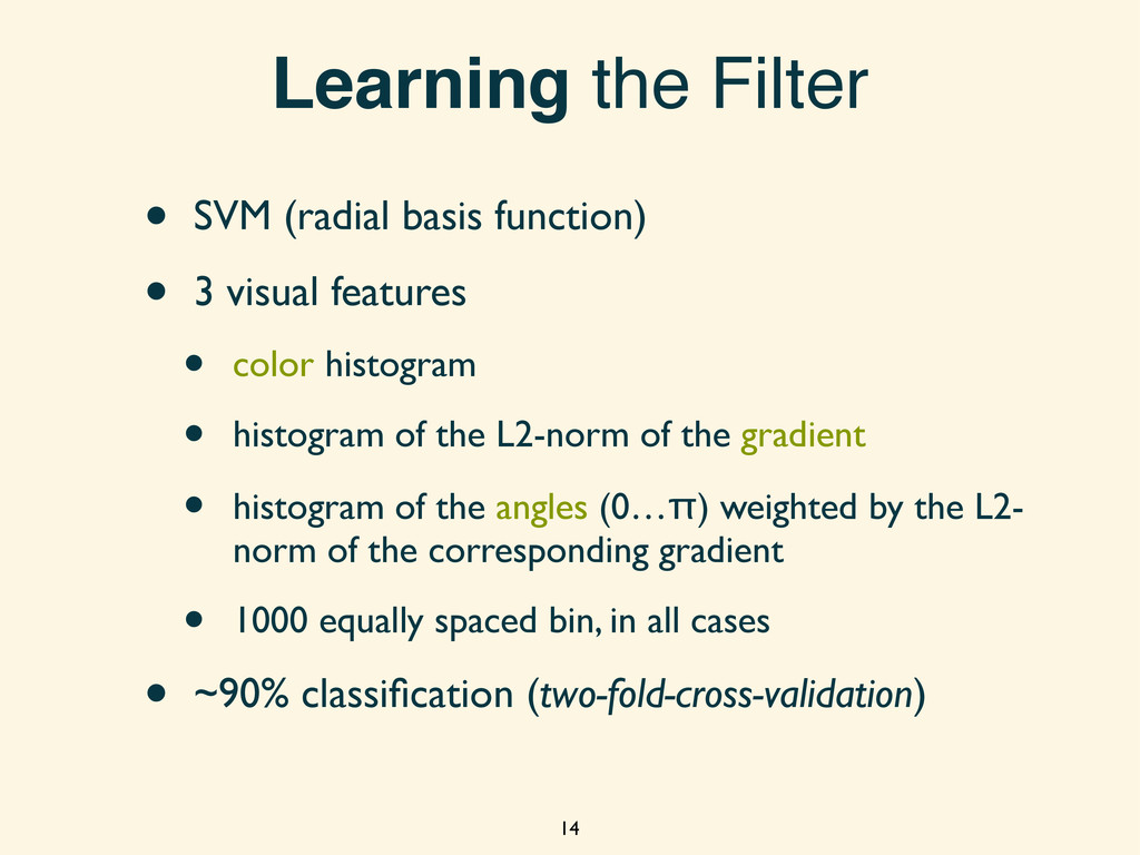
visual features • color histogram • histogram of the L2-norm of the gradient • histogram of the angles (0…π) weighted by the L2- norm of the corresponding gradient • 1000 equally spaced bin, in all cases • ~90% classification (two-fold-cross-validation) 14
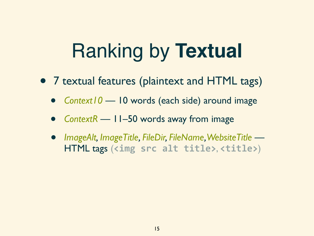
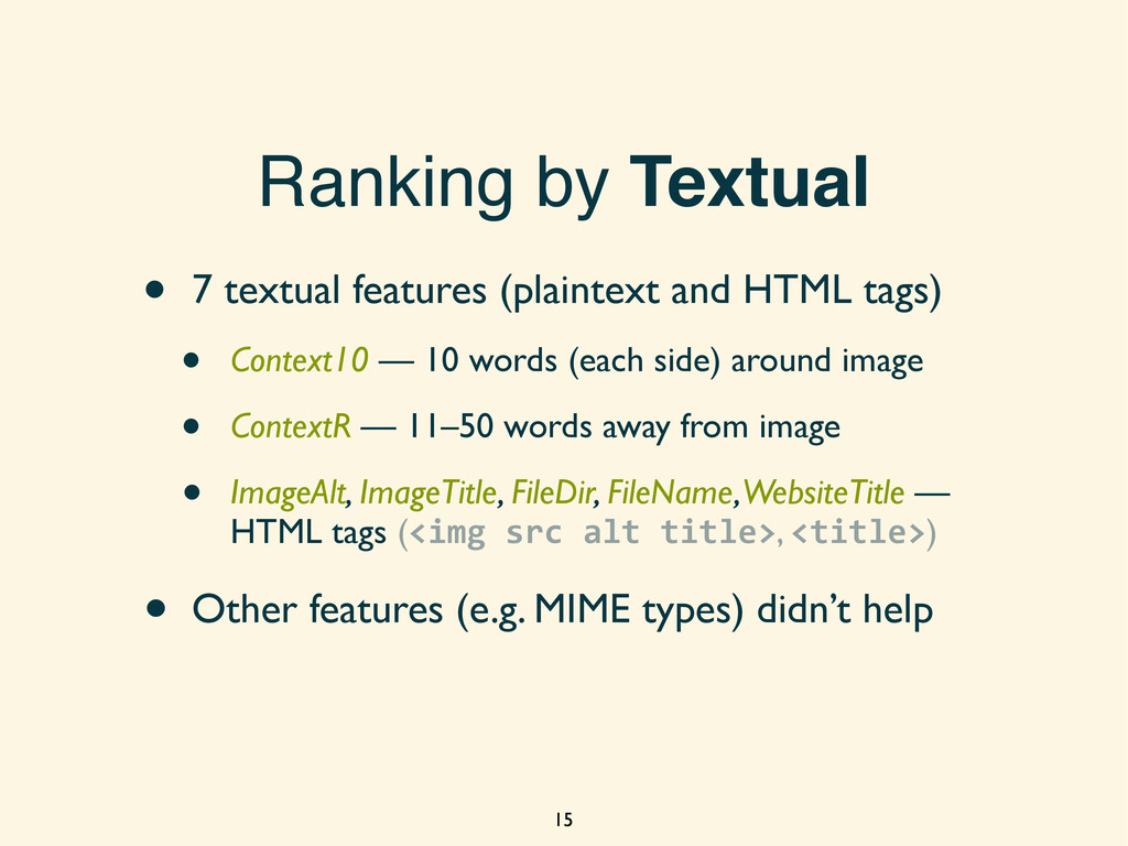
tags) • Context10 — 10 words (each side) around image • ContextR — 11–50 words away from image • ImageAlt, ImageTitle, FileDir, FileName, WebsiteTitle — HTML tags (<img src alt title>, <title>) • Other features (e.g. MIME types) didn’t help 15
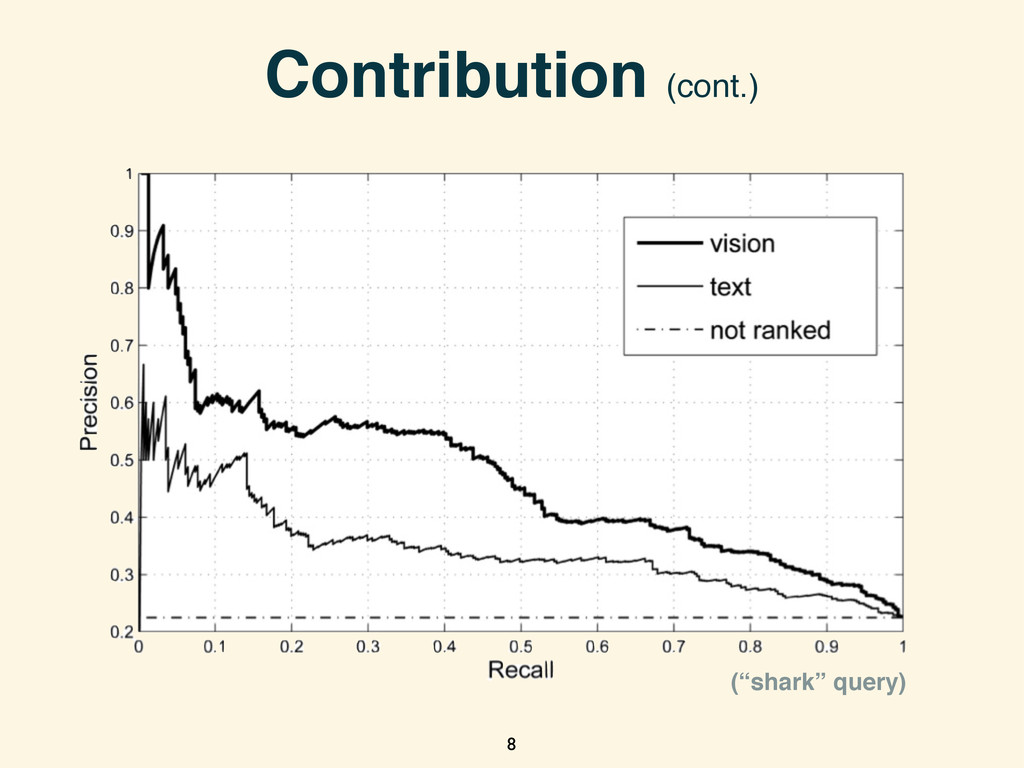
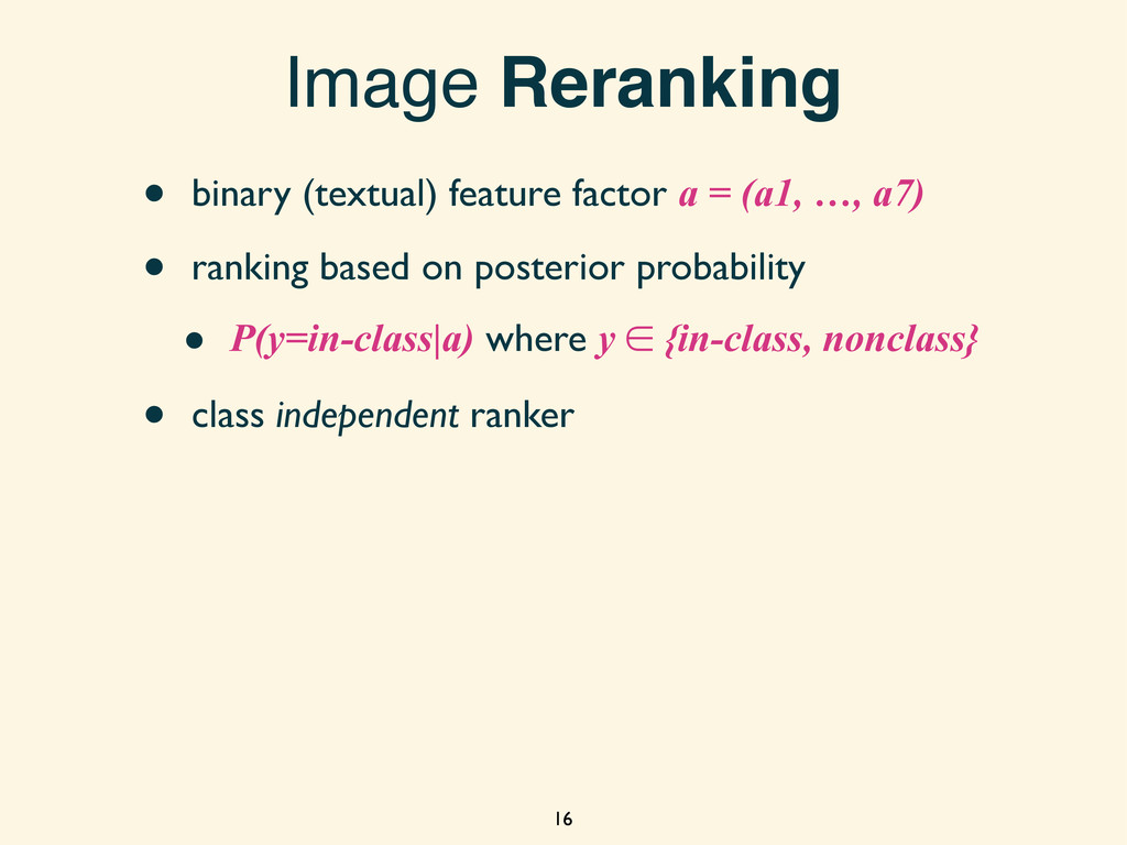
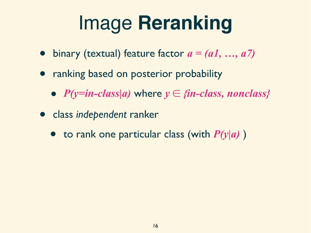
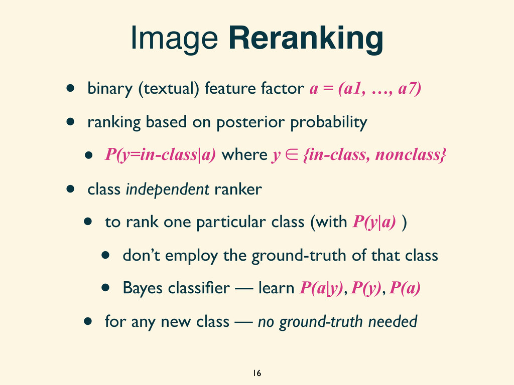
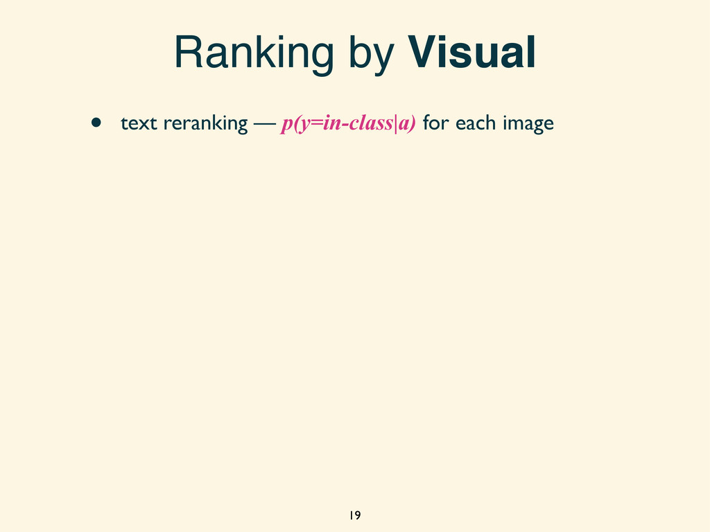
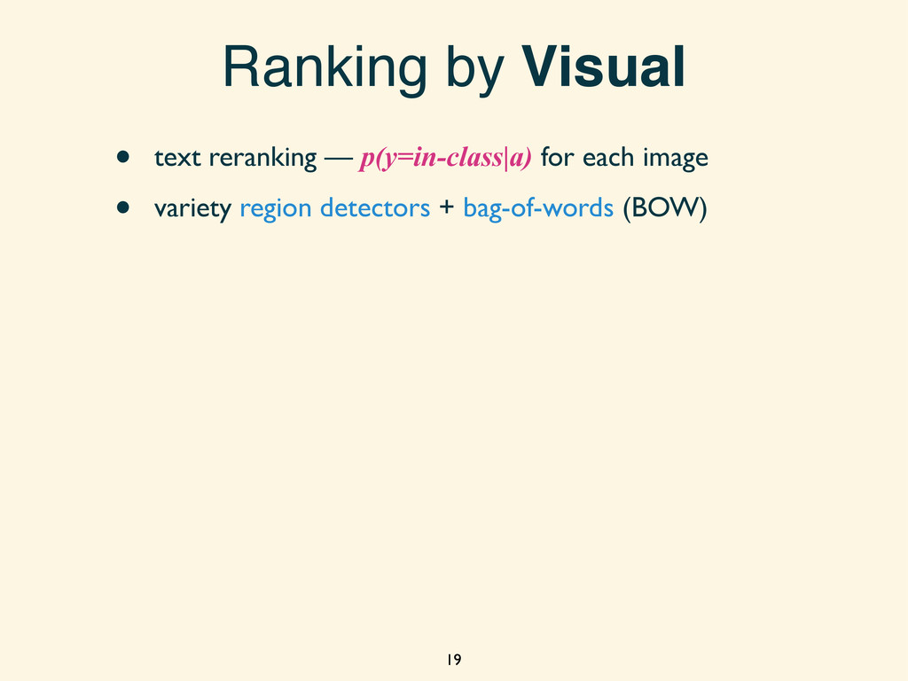
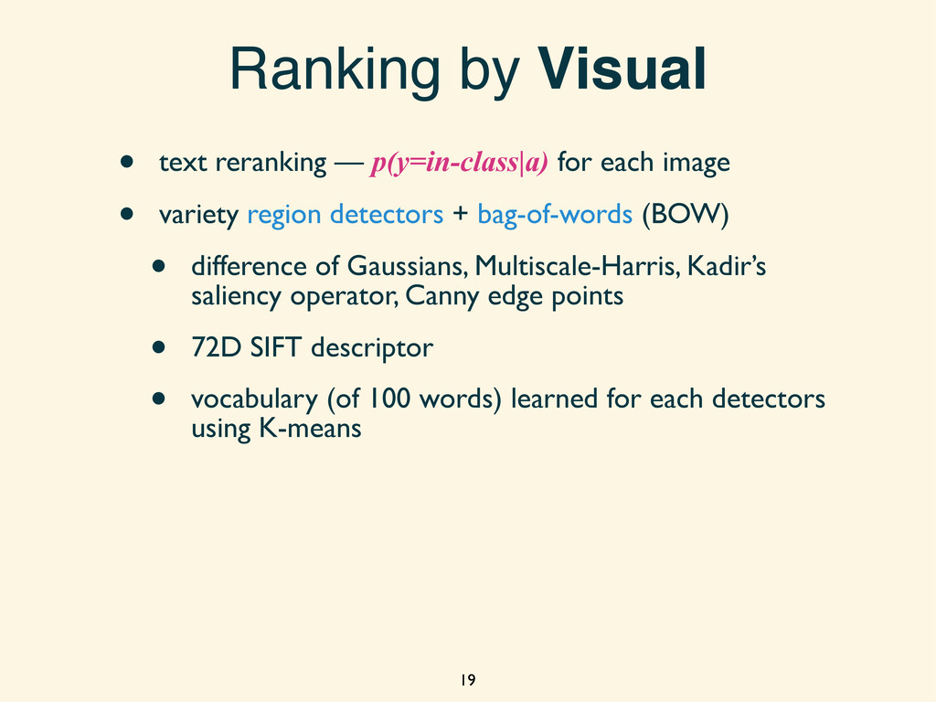
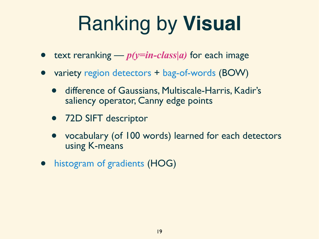
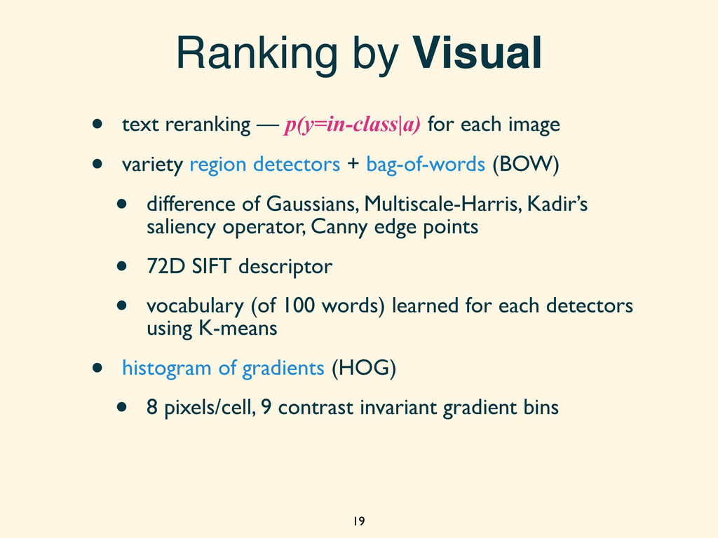
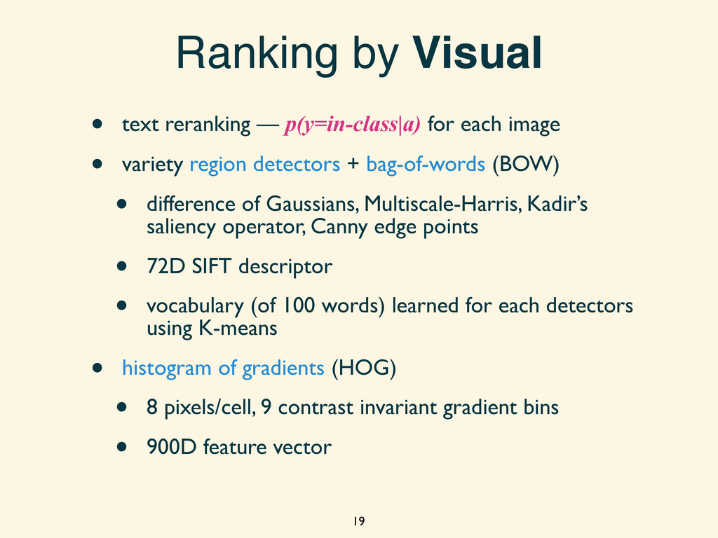
• ranking based on posterior probability • P(y=in-class|a) where y ∈ {in-class, nonclass} • class independent ranker • to rank one particular class (with P(y|a) ) 16 Image Reranking
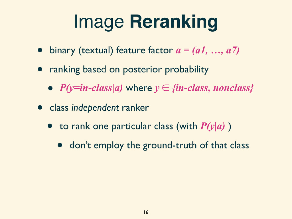
• ranking based on posterior probability • P(y=in-class|a) where y ∈ {in-class, nonclass} • class independent ranker • to rank one particular class (with P(y|a) ) • don’t employ the ground-truth of that class 16 Image Reranking
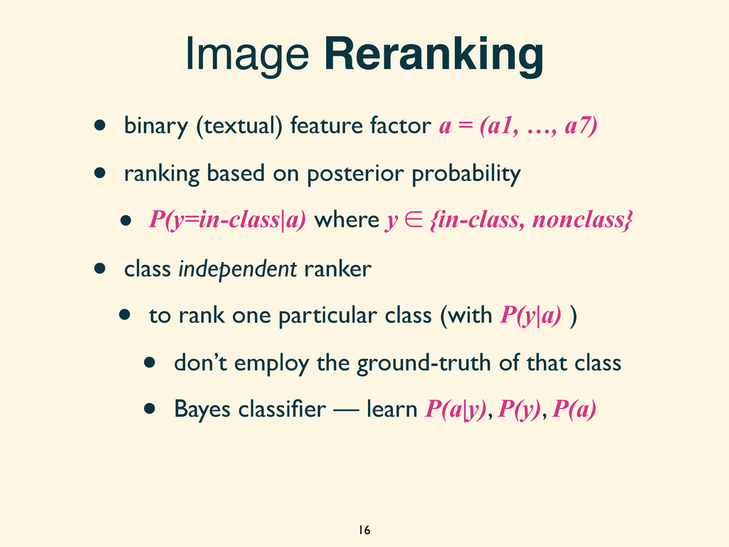
• ranking based on posterior probability • P(y=in-class|a) where y ∈ {in-class, nonclass} • class independent ranker • to rank one particular class (with P(y|a) ) • don’t employ the ground-truth of that class • Bayes classifier — learn P(a|y), P(y), P(a) 16 Image Reranking
• ranking based on posterior probability • P(y=in-class|a) where y ∈ {in-class, nonclass} • class independent ranker • to rank one particular class (with P(y|a) ) • don’t employ the ground-truth of that class • Bayes classifier — learn P(a|y), P(y), P(a) • for any new class — no ground-truth needed 16 Image Reranking
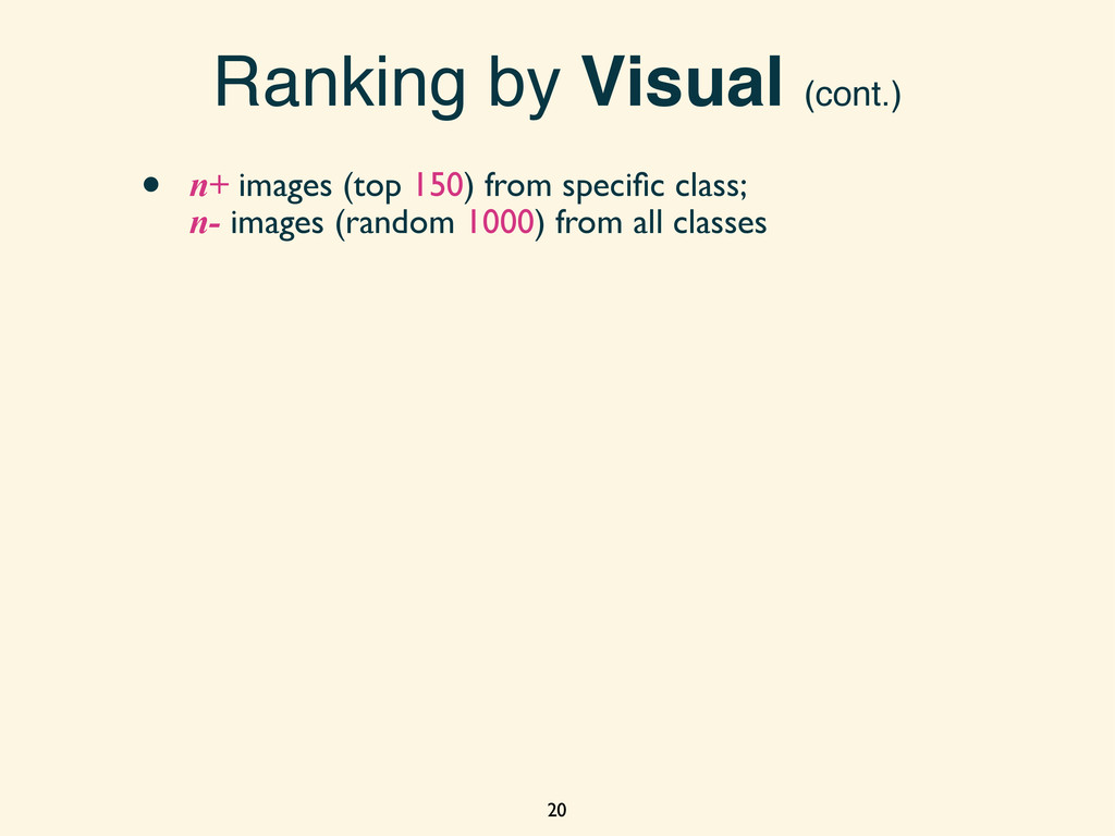
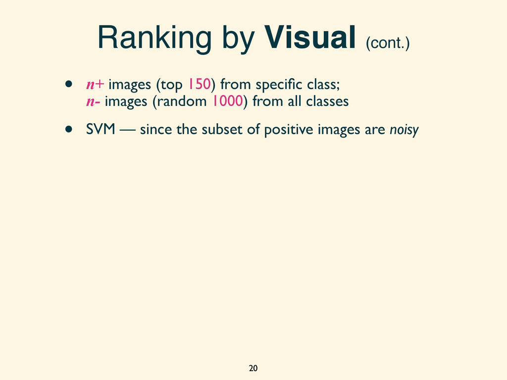
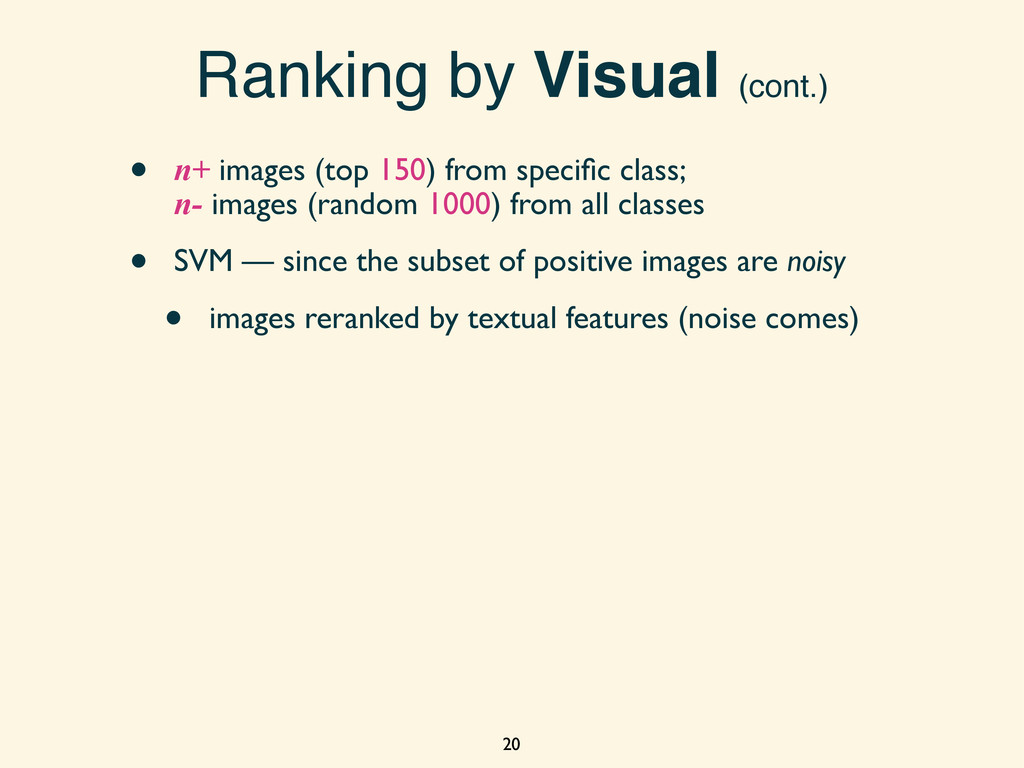
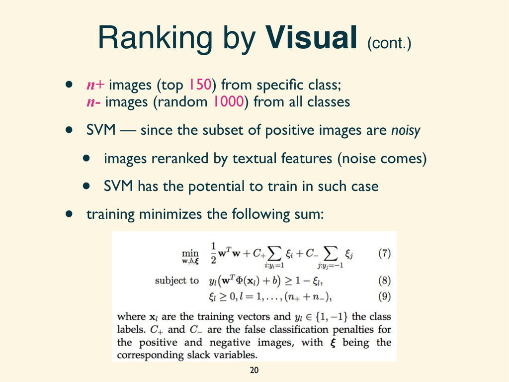
specific class; n- images (random 1000) from all classes • SVM — since the subset of positive images are noisy • images reranked by textual features (noise comes) 20
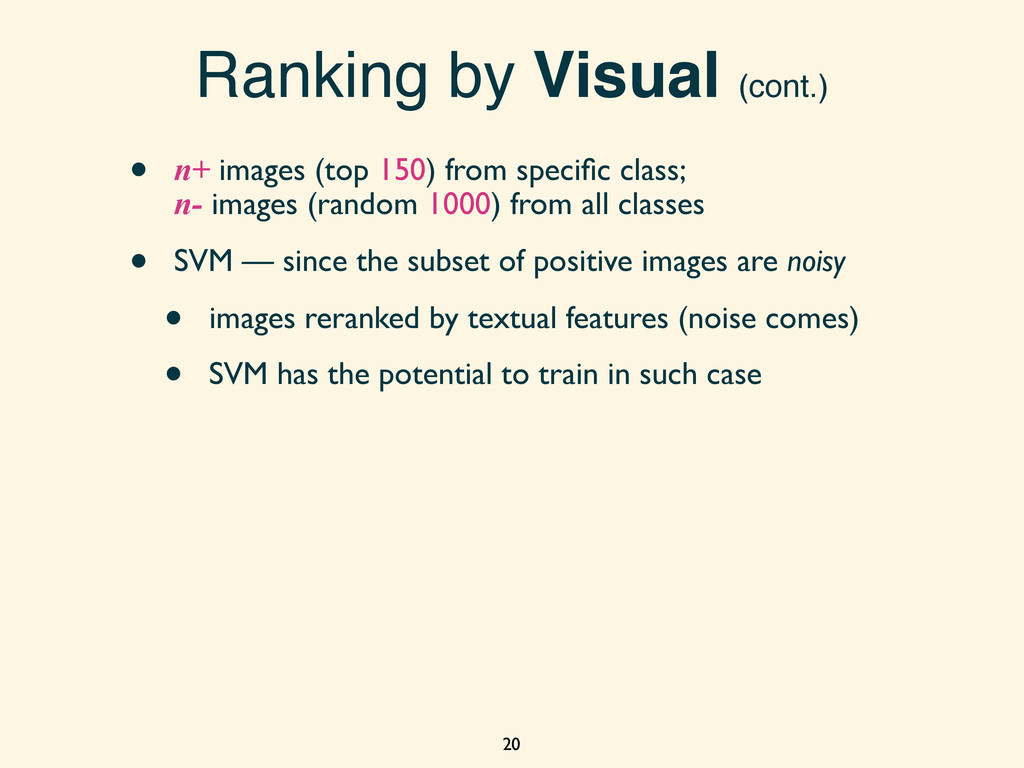
specific class; n- images (random 1000) from all classes • SVM — since the subset of positive images are noisy • images reranked by textual features (noise comes) • SVM has the potential to train in such case 20
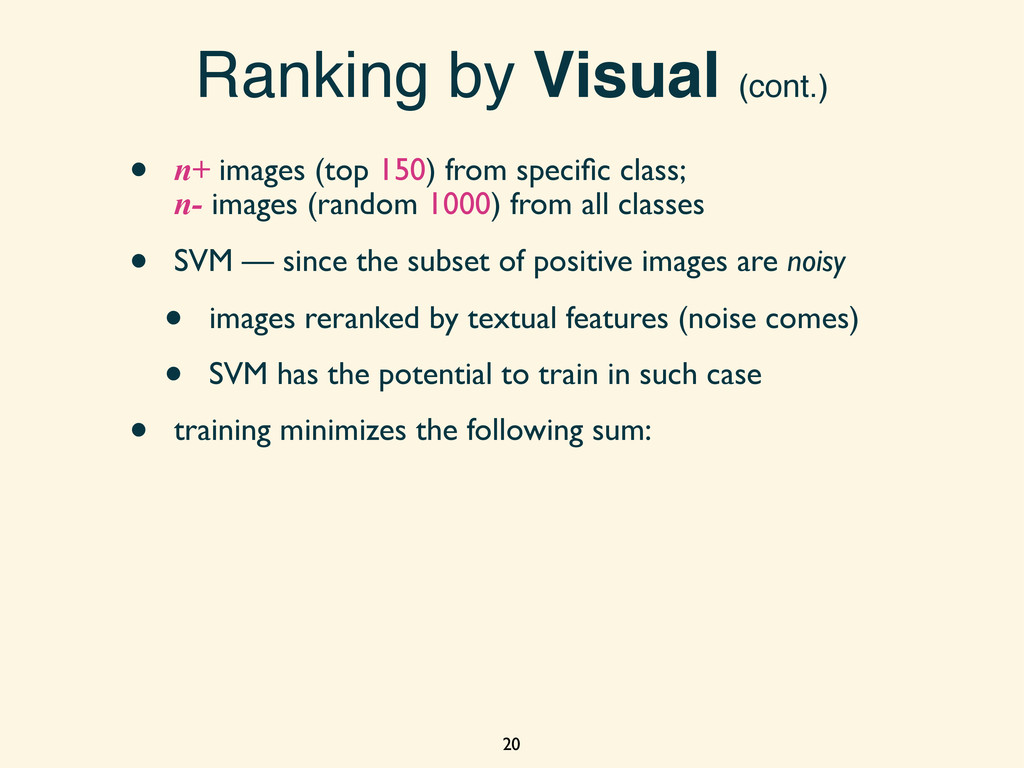
specific class; n- images (random 1000) from all classes • SVM — since the subset of positive images are noisy • images reranked by textual features (noise comes) • SVM has the potential to train in such case • training minimizes the following sum: 20
specific class; n- images (random 1000) from all classes • SVM — since the subset of positive images are noisy • images reranked by textual features (noise comes) • SVM has the potential to train in such case • training minimizes the following sum: 20
images of a given query class • polysemy and diffuseness are difficult to handle • future work • leverage multimodal visual models • different clusters of polysemous meanings 24
images of a given query class • polysemy and diffuseness are difficult to handle • future work • leverage multimodal visual models • different clusters of polysemous meanings • “tiger” — the animal, Tiger Woods 24
images of a given query class • polysemy and diffuseness are difficult to handle • future work • leverage multimodal visual models • different clusters of polysemous meanings • “tiger” — the animal, Tiger Woods • divide diffuse categories 24
images of a given query class • polysemy and diffuseness are difficult to handle • future work • leverage multimodal visual models • different clusters of polysemous meanings • “tiger” — the animal, Tiger Woods • divide diffuse categories • “airplane” — airports, airplane interior, ... 24