Bag of Visual Words

Introduction to BoW models

Transcript

1. Bag-of-Words Representation: Principles and Algorithms Désiré Sidibé Assistant Professor - Université de Bourgogne LE2I - UMR CNRS 6306 dro-desire.sidibe@u-bourgogne.fr 25/06/2015 Désiré Sidibé (Le2i) Le2i - Lab Seminar 25/06/2015 1 / 36
2. Outline 1 Introduction 2 BoW representation 3 Improvements & Extensions 4 Conclusion Désiré Sidibé (Le2i) Le2i - Lab Seminar 25/06/2015 2 / 36
3. Outline 1 Introduction 2 BoW representation 3 Improvements & Extensions 4 Conclusion Désiré Sidibé (Le2i) Le2i - Lab Seminar 25/06/2015 3 / 36
4. Bag-of-Words A bit of history The Bag-of-Words (BoW) concept comes from text/documents retrieval community Assume you have to organize web pages into categories Categories include Sports, Movies, Cooking Your goal is to asssign each new webpage to one of these categories You look for certain words in the webpages For example, you might count how many times the word ’game’ appears in the webpage, or how many times the word ’recipe’ appears. Then, you can assign a category based on the frequency of the words The set of words is called a dictionary And each webpage is represented by a bag of words from the dictionary Désiré Sidibé (Le2i) Le2i - Lab Seminar 25/06/2015 4 / 36
5. Bag-of-Words A bit of history Analysing a set of N documents, each represented by xn = [xn 1 , . . . , xn D ]T , where xn i counts how many times word i appears in document n D is typically very large and x will be very sparse The term-frequency (TF) is defiend as tfn i = xn i i xn i The inverse-document frequency (IDF)is given by idfi = log N # of documents that contain term i Désiré Sidibé (Le2i) Le2i - Lab Seminar 25/06/2015 5 / 36
6. Bag-of-Words A bit of history Analysing a set of N documents, each represented by xn = [xn 1 , . . . , xn D ]T , where xn i counts how many times word i appears in document n The term-frequency - inverse document frequency (TF-IDF) is given by xn i = tfn i × idfi TF-IDF gives high weight to terms that appear often in a document, but rarely amongst documents. Latent Semantic Analysis Given a set of documents D, the aim of LSA is to form a lower dimensional representation of each document An interpretation is that the principal directions define ’latent topics’ Désiré Sidibé (Le2i) Le2i - Lab Seminar 25/06/2015 6 / 36
7. Bag-of-Words A bit of history This is the idea that was introduced to the computer vision community in the context of image category recognition The two seminal papers are : 1 "Video Google : a text retrieval approach to object matching in videos", Sivic and Zisserman, ICCV 2003 2 "Visual categorization with bag of keypoints", Csurka et al., ECCV Workshop 2004 Paper 1 introduced the concept of visual vocabulary and used TF-IDF for retrieval Paper 2 introduced the concept of bag of features (later commonly used as BoW) Désiré Sidibé (Le2i) Le2i - Lab Seminar 25/06/2015 7 / 36
8. Bag-of-Words Key issues How to construct a visual dictionary ? Désiré Sidibé (Le2i) Le2i - Lab Seminar 25/06/2015 8 / 36
9. Bag-of-Words Key issues Vocabulary size ? Sampling strategy ? Clustering/Quantization ? Unsupervised vs Supervised ? Désiré Sidibé (Le2i) Le2i - Lab Seminar 25/06/2015 9 / 36
10. Outline 1 Introduction 2 BoW representation 3 Improvements & Extensions 4 Conclusion Désiré Sidibé (Le2i) Le2i - Lab Seminar 25/06/2015 10 / 36
11. BoW representation Local Features Many local features can be used Désiré Sidibé (Le2i) Le2i - Lab Seminar 25/06/2015 11 / 36
12. BoW representation Sampling strategy Keypoints detection Detect a set of keypoints (Harris, SIFT, etc) Extract local descriptors around each keypoint Désiré Sidibé (Le2i) Le2i - Lab Seminar 25/06/2015 12 / 36
13. BoW representation Sampling strategy Dense sampling Divide image into local patches Extract local features from each patch Désiré Sidibé (Le2i) Le2i - Lab Seminar 25/06/2015 13 / 36
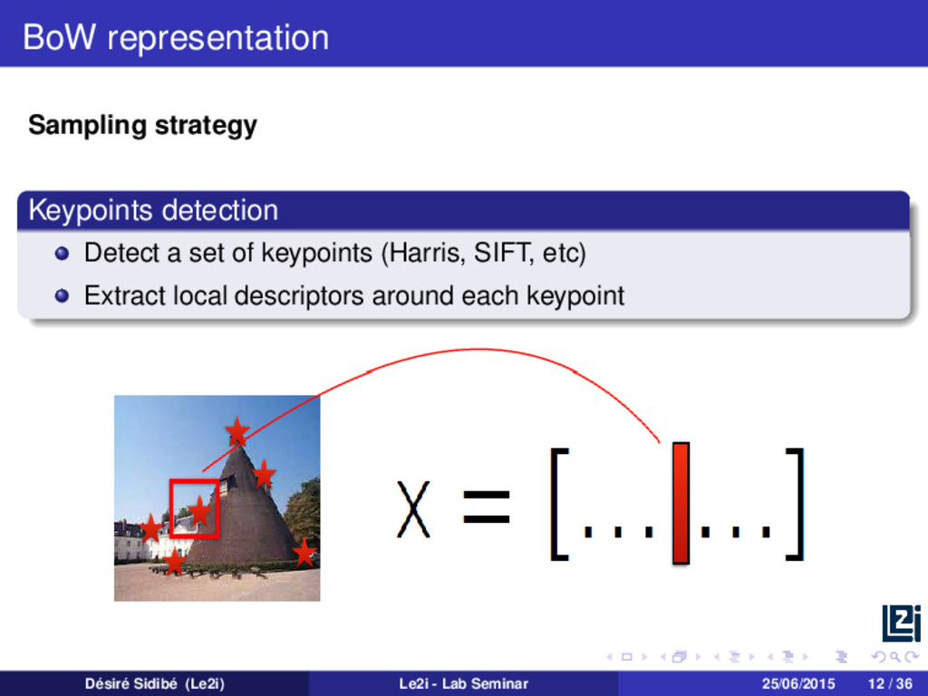
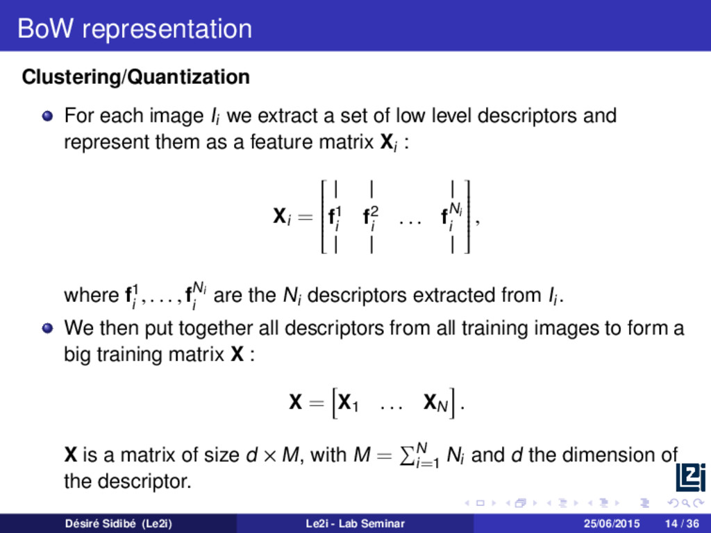
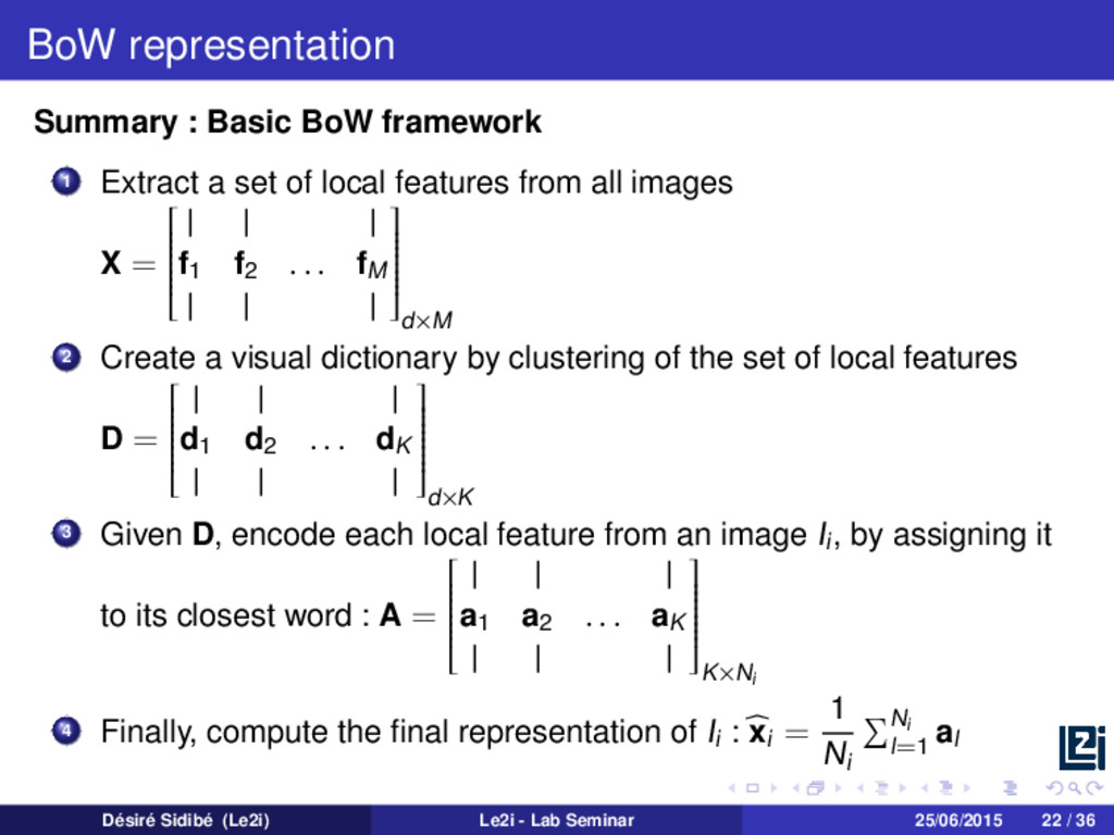
14. BoW representation Clustering/Quantization For each image Ii we extract a set of low level descriptors and represent them as a feature matrix Xi : Xi =           | | | f1 i f2 i . . . fNi i | | |           , where f1 i , . . . , fNi i are the Ni descriptors extracted from Ii. We then put together all descriptors from all training images to form a big training matrix X : X = X1 . . . XN . X is a matrix of size d × M, with M = N i=1 Ni and d the dimension of the descriptor. Désiré Sidibé (Le2i) Le2i - Lab Seminar 25/06/2015 14 / 36
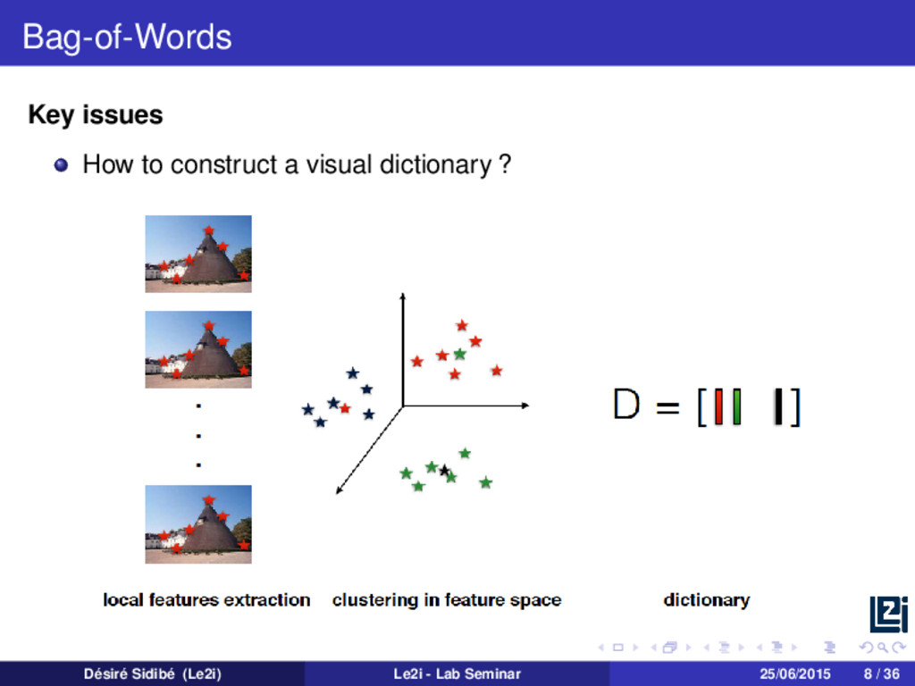
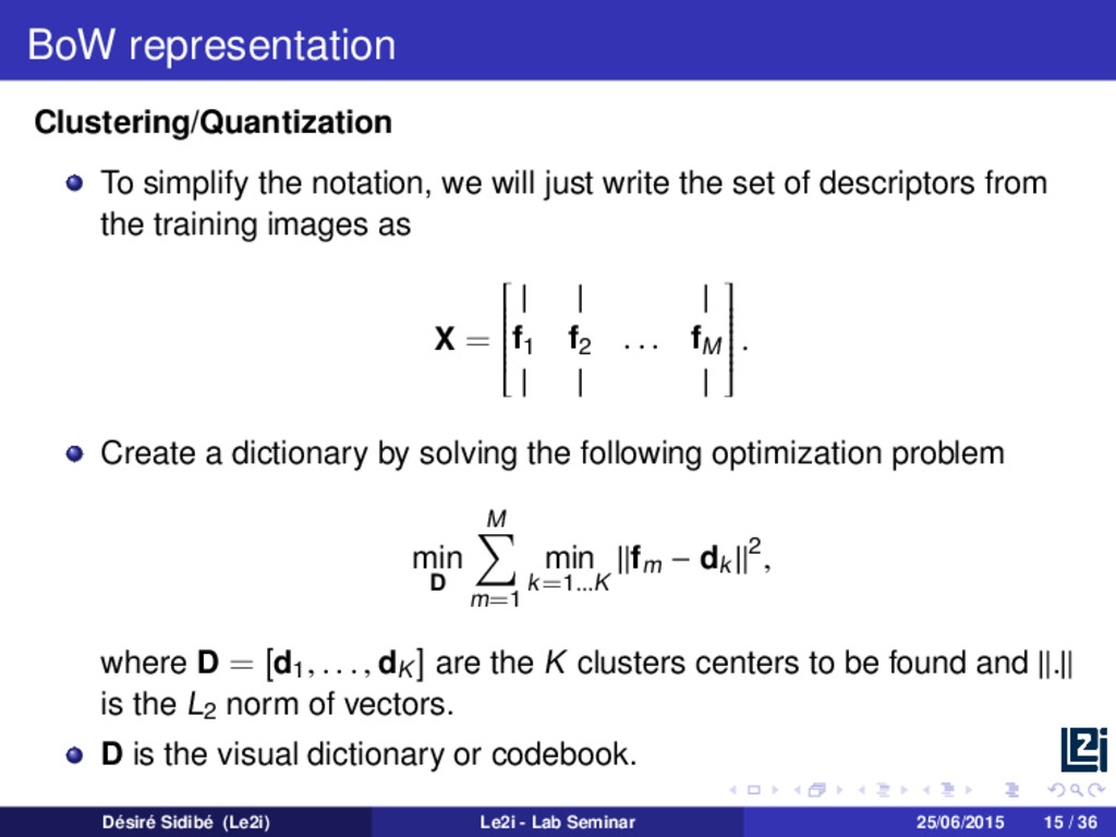
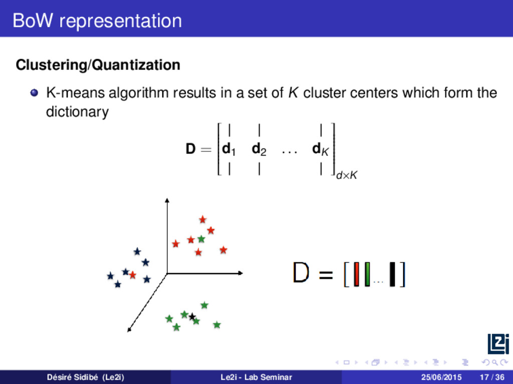
15. BoW representation Clustering/Quantization To simplify the notation, we will just write the set of descriptors from the training images as X =           | | | f1 f2 . . . fM | | |           . Create a dictionary by solving the following optimization problem min D M m=1 min k=1...K fm − dk 2, where D = [d1 , . . . , dK ] are the K clusters centers to be found and . is the L2 norm of vectors. D is the visual dictionary or codebook. Désiré Sidibé (Le2i) Le2i - Lab Seminar 25/06/2015 15 / 36
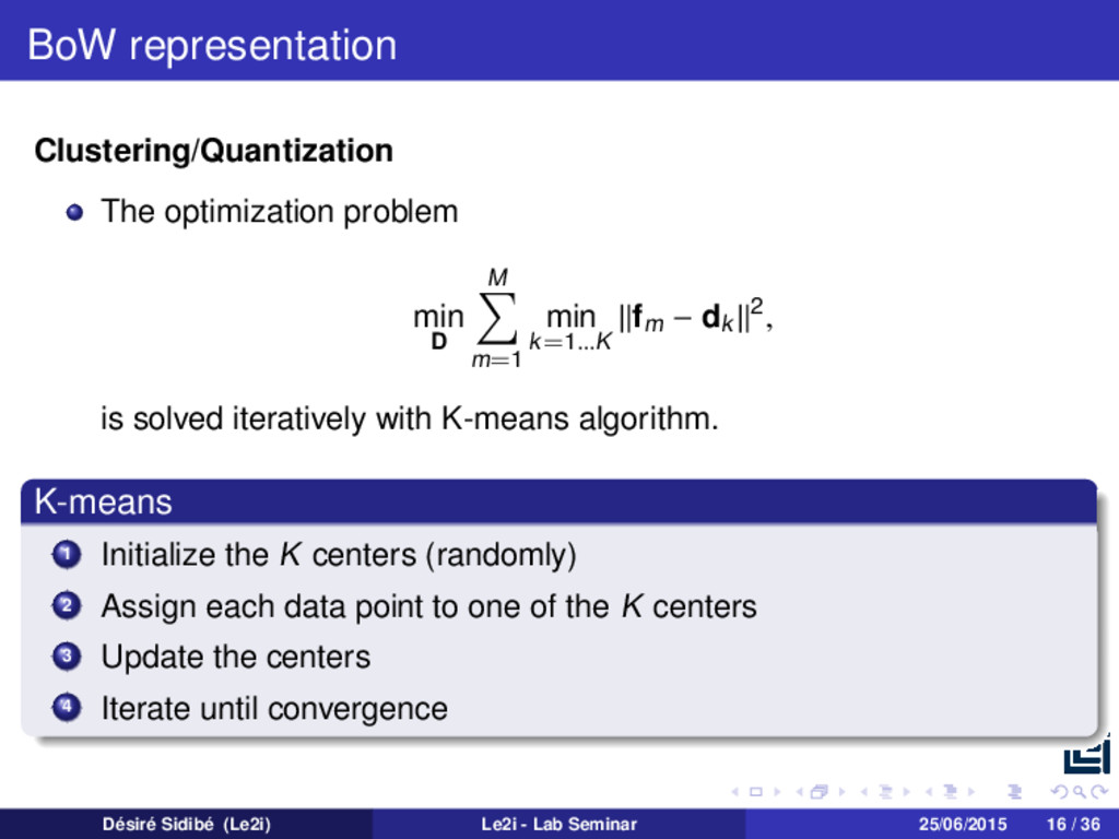
16. BoW representation Clustering/Quantization The optimization problem min D M m=1 min k=1...K fm − dk 2, is solved iteratively with K-means algorithm. K-means 1 Initialize the K centers (randomly) 2 Assign each data point to one of the K centers 3 Update the centers 4 Iterate until convergence Désiré Sidibé (Le2i) Le2i - Lab Seminar 25/06/2015 16 / 36
17. BoW representation Clustering/Quantization K-means algorithm results in a set of K cluster centers which form the dictionary D =           | | | d1 d2 . . . dK | | |           d×K Désiré Sidibé (Le2i) Le2i - Lab Seminar 25/06/2015 17 / 36
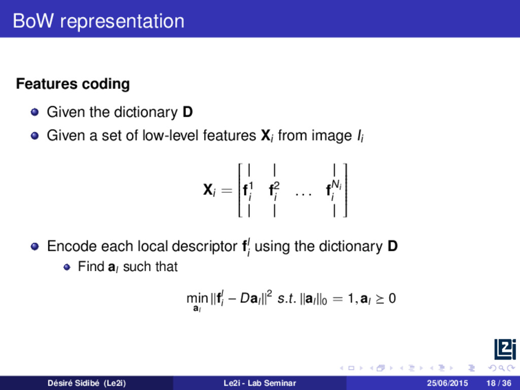
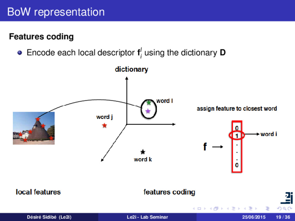
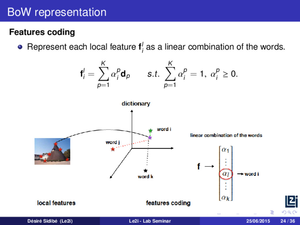
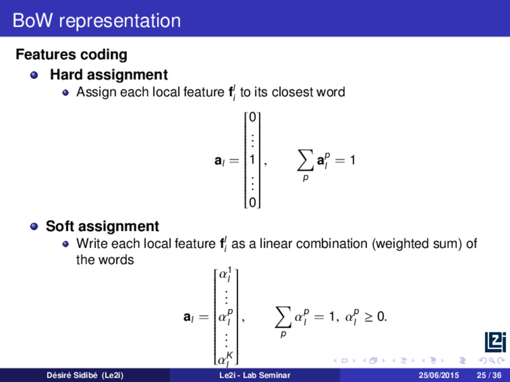
18. BoW representation Features coding Given the dictionary D Given a set of low-level features Xi from image Ii Xi =           | | | f1 i f2 i . . . fNi i | | |           Encode each local descriptor fl i using the dictionary D Find al such that min al fl i − Dal 2 s.t. al 0 = 1, al 0 Désiré Sidibé (Le2i) Le2i - Lab Seminar 25/06/2015 18 / 36
19. BoW representation Features coding Encode each local descriptor fl i using the dictionary D Désiré Sidibé (Le2i) Le2i - Lab Seminar 25/06/2015 19 / 36
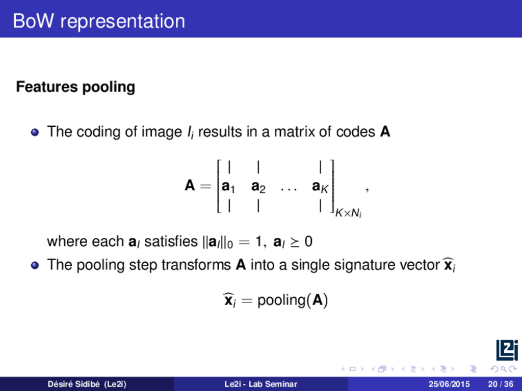
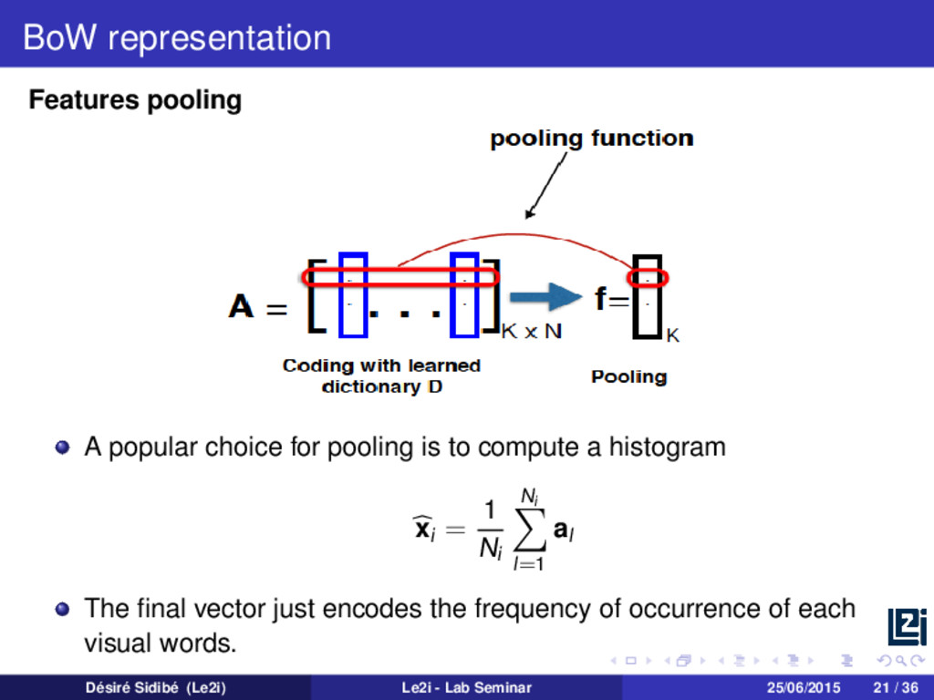
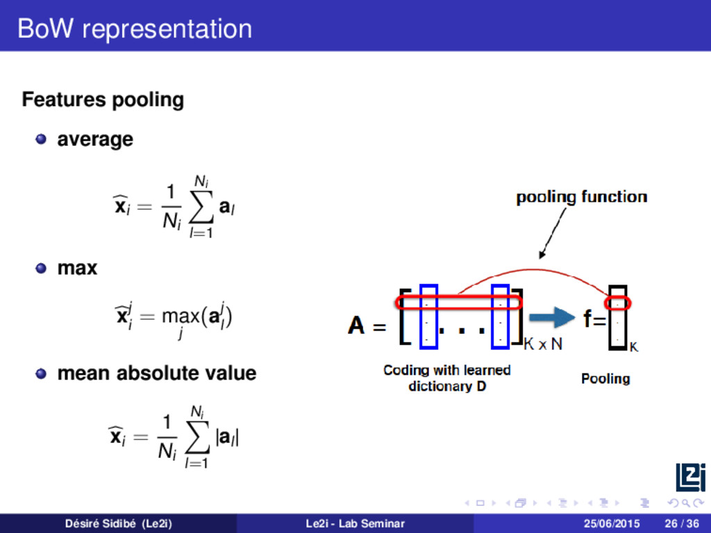
20. BoW representation Features pooling The coding of image Ii results in a matrix of codes A A =           | | | a1 a2 . . . aK | | |           K×Ni , where each al satisfies al 0 = 1, al 0 The pooling step transforms A into a single signature vector xi xi = pooling(A) Désiré Sidibé (Le2i) Le2i - Lab Seminar 25/06/2015 20 / 36
21. BoW representation Features pooling A popular choice for pooling is to compute a histogram xi = 1 Ni Ni l=1 al The final vector just encodes the frequency of occurrence of each visual words. Désiré Sidibé (Le2i) Le2i - Lab Seminar 25/06/2015 21 / 36
22. BoW representation Summary : Basic BoW framework 1 Extract a set of local features from all images X =           | | | f1 f2 . . . fM | | |           d×M 2 Create a visual dictionary by clustering of the set of local features D =           | | | d1 d2 . . . dK | | |           d×K 3 Given D, encode each local feature from an image Ii, by assigning it to its closest word : A =           | | | a1 a2 . . . aK | | |           K×Ni 4 Finally, compute the final representation of Ii : xi = 1 Ni Ni l=1 al Désiré Sidibé (Le2i) Le2i - Lab Seminar 25/06/2015 22 / 36
23. Outline 1 Introduction 2 BoW representation 3 Improvements & Extensions 4 Conclusion Désiré Sidibé (Le2i) Le2i - Lab Seminar 25/06/2015 23 / 36
24. BoW representation Features coding Represent each local feature fl i as a linear combination of the words. fl i = K p=1 αp i dp s.t. K p=1 αp i = 1, αp i ≥ 0. Désiré Sidibé (Le2i) Le2i - Lab Seminar 25/06/2015 24 / 36
25. BoW representation Features coding Hard assignment Assign each local feature fl i to its closest word al =                          0 . . . 1 . . . 0                          , p ap l = 1 Soft assignment Write each local feature fl i as a linear combination (weighted sum) of the words al =                          α1 l . . . αp l . . . αK l                          , p αp l = 1, αp l ≥ 0. Désiré Sidibé (Le2i) Le2i - Lab Seminar 25/06/2015 25 / 36
26. BoW representation Features pooling average xi = 1 Ni Ni l=1 al max xj i = max j (aj l ) mean absolute value xi = 1 Ni Ni l=1 |al| Désiré Sidibé (Le2i) Le2i - Lab Seminar 25/06/2015 26 / 36
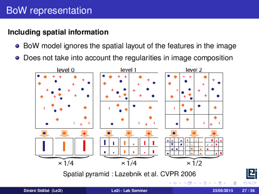
27. BoW representation Including spatial information BoW model ignores the spatial layout of the features in the image Does not take into account the regularities in image composition Spatial pyramid : Lazebnik et al. CVPR 2006 Désiré Sidibé (Le2i) Le2i - Lab Seminar 25/06/2015 27 / 36
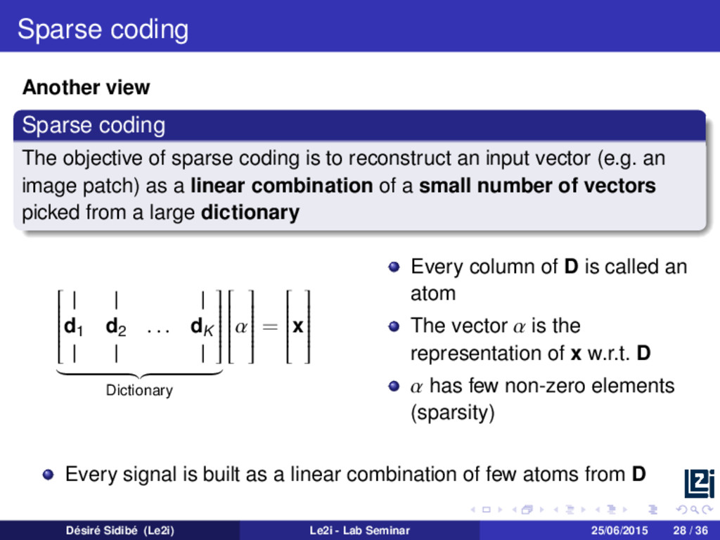
28. Sparse coding Another view Sparse coding The objective of sparse coding is to reconstruct an input vector (e.g. an image patch) as a linear combination of a small number of vectors picked from a large dictionary           | | | d1 d2 . . . dK | | |           Dictionary           α           =           x           Every column of D is called an atom The vector α is the representation of x w.r.t. D α has few non-zero elements (sparsity) Every signal is built as a linear combination of few atoms from D Désiré Sidibé (Le2i) Le2i - Lab Seminar 25/06/2015 28 / 36
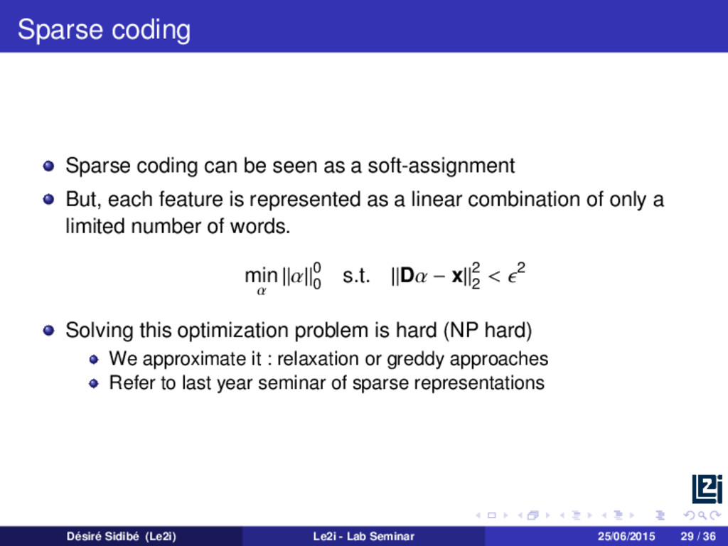
29. Sparse coding Sparse coding can be seen as a soft-assignment But, each feature is represented as a linear combination of only a limited number of words. min α α 0 0 s.t. Dα − x 2 2 < 2 Solving this optimization problem is hard (NP hard) We approximate it : relaxation or greddy approaches Refer to last year seminar of sparse representations Désiré Sidibé (Le2i) Le2i - Lab Seminar 25/06/2015 29 / 36
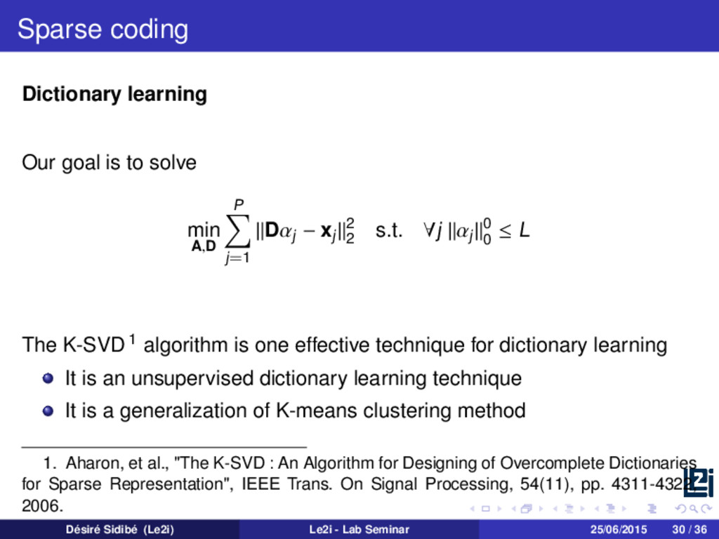
30. Sparse coding Dictionary learning Our goal is to solve min A,D P j=1 Dαj − xj 2 2 s.t. ∀j αj 0 0 ≤ L The K-SVD 1 algorithm is one effective technique for dictionary learning It is an unsupervised dictionary learning technique It is a generalization of K-means clustering method 1. Aharon, et al., "The K-SVD : An Algorithm for Designing of Overcomplete Dictionaries for Sparse Representation", IEEE Trans. On Signal Processing, 54(11), pp. 4311-4322, 2006. Désiré Sidibé (Le2i) Le2i - Lab Seminar 25/06/2015 30 / 36
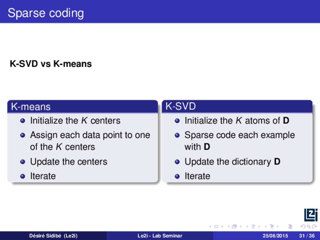
31. Sparse coding K-SVD vs K-means K-means Initialize the K centers Assign each data point to one of the K centers Update the centers Iterate K-SVD Initialize the K atoms of D Sparse code each example with D Update the dictionary D Iterate Désiré Sidibé (Le2i) Le2i - Lab Seminar 25/06/2015 31 / 36
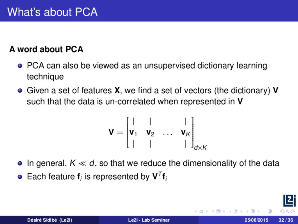
32. What’s about PCA A word about PCA PCA can also be viewed as an unsupervised dictionary learning technique Given a set of features X, we find a set of vectors (the dictionary) V such that the data is un-correlated when represented in V V =           | | | v1 v2 . . . vK | | |           d×K In general, K d, so that we reduce the dimensionality of the data Each feature fi is represented by VT fi Désiré Sidibé (Le2i) Le2i - Lab Seminar 25/06/2015 32 / 36
33. What’s about PCA A word about PCA PCA finds a set of K vectors such that K ≤ d When K < d, we say that we have an under-complete dictionary When K = d, we say that we have a complete dictionary With the BoW approach, we will usually have large dictionaries, K > d When K > d, we say that we have an over-complete dictionary Désiré Sidibé (Le2i) Le2i - Lab Seminar 25/06/2015 33 / 36
34. Conclusions From a broader perspective Matrix factorization Decomposing each input example as a linear combination of basis vectors X ≈ DA PCA variance maximization ICA non-Gaussianity (kurtosis) maximization NMF non-negativity constraints Sparse coding sparsity constraints ... Table : Different approaches Désiré Sidibé (Le2i) Le2i - Lab Seminar 25/06/2015 34 / 36
35. Outline 1 Introduction 2 BoW representation 3 Improvements & Extensions 4 Conclusion Désiré Sidibé (Le2i) Le2i - Lab Seminar 25/06/2015 35 / 36
36. Conclusions The BoW approach is an efficient image representation technique It is inspired by ideas from text/documents retrieval community Many extensions and improvements have been proposed Including spatial layout : spatial pyramid It falls within a more general framework Désiré Sidibé (Le2i) Le2i - Lab Seminar 25/06/2015 36 / 36