GB WhatsApp APK Download | Anti-Ban Official GBWhatsApp 2025

gbwhata is a modified version of the official WhatsApp application, offering advanced features such as enhanced privacy options, customization capabilities, and the ability to share larger media files, providing users with a more versatile messaging experience.

Transcript

1. Ocean wave model output parameters Jean-Raymond Bidlot ECMWF jean.bidlot@ecmwf.int February 27, 2020 1 Introduction This document gives a short summary of the definition of ECMWF ocean wave model output param- eters. Please refer to the official IFS documentation part VII for a full description of the wave model (https://software.ecmwf.int/wiki/display/IFS/Official+IFS+Documentation). The data are encoded in grib, edition 1. See table(1) for the full list of all available parameters 2 Wave spectra There are two quantities that are actually computed at each grid point of the wave model, namely the two- dimensional (2-D) wave spectrum F(f, θ) and the total atmospheric surface stress τa for a given atmospheric forcing. In its continuous form, F(f, θ) describes how the wave energy is distributed as function of frequency f and propagation direction θ. In the numerical implementation of the wave model, F is discretised using nfre frequencies and nang directions. In the current analysis and deterministic forecast configuration nfre = 36 and nang = 36. Whenever possible, F(f, θ) is output and archived as parameter 251. It corresponds to the full description of the wave field at any grid point. It is however a very cumbersome quantity to plot as a full field since it consists of nfre × nang values at each grid point. Nevertheless, it can plotted for specific locations. Figures 1 and 2 display the spectra at 6 different locations as indicated on Figure 3 (model bathymetry, parameter 219 is also shown). The two-dimensional wave spectrum is represented using a polar plot reprsentation, where the radial coordinate represents frequency and the polar direction is the propagation direction of each wave component. The oceanographic convention is used, such that upwards indicates that waves are propagating to the North. The frequency spectrum, which indicates how wave energy is distributed in frequency, is obtained by integrating over all directions. From Figure 1, it clear that for many locations, the sea state is composed of many different wave systems. 3 Integral parameters describing the wave field In order to simplify the study of wave conditions, integral parameters are computed from some weighted integrals of F(f, θ) or its source terms. It is quite often customary to differentiate the wave components in the spectrum as windsea (or wind waves) and swell. Here, windsea is defined as those wave components that are still subject to wind forcing while the remaining part of the spectrum is termed swell, total swell if the full remaining part is considered as one entity or first, second or third swell partition when it is split into the 3 most energetic systems (see section on swell partitioning). To a good approximation, spectral components are considered to be subject to forcing by the wind when 1.2 × 28(u∗ /c) cos(θ − φ) > 1 (1) where u∗ is the friction velocity (u2 ∗ = τa ρair ), ρair the surface air density, c = c(f) is the phase speed as derived from the linear theory of waves and φ is the wind direction. The integrated parameters are therefore also computed for windsea and swell by only integrating over the respective components of F(f, θ) that satisfies (1) or not (for windsea and total swell) or by integrating over the part of the spectrum that has been identified to belong to the first, second or third swell partition. Let us define the moment of order n of F, mn as the integral mn = dfdθ fnF(f, θ) (2) 1
2. 0 3 6 9 12 15 18 21 E(f) (m^2 s) 0 0.1 0.2 0.3 0.4 0.5 0.6 0.7 0.8 0.9 Frequency (Hz) Concentric circles are every 0.05 Hz North is pointing upwards Propagation direction is with respect to North MWD = 156 degrees PWD = 170 degrees Peakedness Qp = 1.23, Directional Spread = 0.99 Hs= 4.17 m, Tm= 10.50 s, Tp= 12.29 s at P0011 ( 66.00 , -10.00 ) 06:00Z on 27.03.2016 NORMALISED 2-D SPECTRUM for 0001 wave od Normalised spectrum 0.00 0.04 0.06 0.08 0.13 0.19 0.28 0.43 0.64 0.96 1.00 (a) point 11 0 3 6 9 12 15 E(f) (m^2 s) 0 0.1 0.2 0.3 0.4 0.5 0.6 0.7 0.8 0.9 Frequency (Hz) Concentric circles are every 0.05 Hz North is pointing upwards Propagation direction is with respect to North MWD = 36 degrees PWD = 60 degrees Peakedness Qp = 1.53, Directional Spread = 0.68 Hs= 3.66 m, Tm= 11.10 s, Tp= 13.51 s at P0001 ( 66.00 , 0.00 ) 06:00Z on 27.03.2016 NORMALISED 2-D SPECTRUM for 0001 wave od Normalised spectrum 0.00 0.04 0.06 0.08 0.13 0.19 0.28 0.43 0.64 0.96 1.00 (b) point 1 0 3 6 9 12 15 18 E(f) (m^2 s) 0 0.1 0.2 0.3 0.4 0.5 0.6 0.7 0.8 0.9 Frequency (Hz) Concentric circles are every 0.05 Hz North is pointing upwards Propagation direction is with respect to North MWD = 84 degrees PWD = 50 degrees Peakedness Qp = 0.99, Directional Spread = 0.92 Hs= 4.09 m, Tm= 10.62 s, Tp= 12.29 s at P0012 ( 64.00 , -10.00 ) 06:00Z on 27.03.2016 NORMALISED 2-D SPECTRUM for 0001 wave od Normalised spectrum 0.00 0.04 0.06 0.08 0.13 0.19 0.28 0.43 0.64 0.96 1.00 (c) point 12 0 3 6 9 12 E(f) (m^2 s) 0 0.1 0.2 0.3 0.4 0.5 0.6 0.7 0.8 0.9 Frequency (Hz) Concentric circles are every 0.05 Hz North is pointing upwards Propagation direction is with respect to North MWD = 16 degrees PWD = 70 degrees Peakedness Qp = 0.94, Directional Spread = 0.68 Hs= 4.35 m, Tm= 9.57 s, Tp= 13.51 s at P0002 ( 64.00 , 0.00 ) 06:00Z on 27.03.2016 NORMALISED 2-D SPECTRUM for 0001 wave od Normalised spectrum 0.00 0.04 0.06 0.08 0.13 0.19 0.28 0.43 0.64 0.96 1.00 (d) point 2 0 3 6 9 12 15 E(f) (m^2 s) 0 0.1 0.2 0.3 0.4 0.5 0.6 0.7 0.8 0.9 Frequency (Hz) Concentric circles are every 0.05 Hz North is pointing upwards Propagation direction is with respect to North MWD = 75 degrees PWD = 60 degrees Peakedness Qp = 1.19, Directional Spread = 0.74 Hs= 3.98 m, Tm= 10.50 s, Tp= 13.51 s at P0013 ( 62.00 , -10.00 ) 06:00Z on 27.03.2016 NORMALISED 2-D SPECTRUM for 0001 wave od Normalised spectrum 0.00 0.04 0.06 0.08 0.13 0.19 0.28 0.43 0.64 0.96 1.00 (e) point 13 0 10 20 30 40 E(f) (m^2 s) 0 0.1 0.2 0.3 0.4 0.5 0.6 0.7 0.8 0.9 Frequency (Hz) Concentric circles are every 0.05 Hz North is pointing upwards Propagation direction is with respect to North MWD = 354 degrees PWD = 340 degrees Peakedness Qp = 1.18, Directional Spread = 0.64 Hs= 6.08 m, Tm= 9.50 s, Tp= 10.15 s at P0003 ( 62.00 , 0.00 ) 06:00Z on 27.03.2016 NORMALISED 2-D SPECTRUM for 0001 wave od Normalised spectrum 0.00 0.04 0.06 0.08 0.13 0.19 0.28 0.43 0.64 0.96 1.00 (f) point 3 Figure 1: Normalised 2d spectra (top of each panel) and frequency spectra (bottom of each panel) on 23 March 2016, 6 UTC, for locations shown in Figure 3. The 2-D spectra were normalised by their respective maximum value. The concentric circles in the polar plots are spaced every 0.05 Hz 2
3. 0 3 6 9 12 15 18 E(f) (m^2 s) 0 0.1 0.2 0.3 0.4 0.5 0.6 0.7 0.8 0.9 Frequency (Hz) Concentric circles are every 0.05 Hz North is pointing upwards Propagation direction is with respect to North MWD = 78 degrees PWD = 60 degrees Peakedness Qp = 1.19, Directional Spread = 0.72 Hs= 4.24 m, Tm= 10.43 s, Tp= 13.51 s at P0014 ( 60.00 , -10.00 ) 06:00Z on 27.03.2016 NORMALISED 2-D SPECTRUM for 0001 wave od Normalised spectrum 0.00 0.04 0.06 0.08 0.13 0.19 0.28 0.43 0.64 0.96 1.00 (a) point 14 0 10 20 30 40 50 E(f) (m^2 s) 0 0.1 0.2 0.3 0.4 0.5 0.6 0.7 0.8 0.9 Frequency (Hz) Concentric circles are every 0.05 Hz North is pointing upwards Propagation direction is with respect to North MWD = 353 degrees PWD = 0 degrees Peakedness Qp = 1.71, Directional Spread = 0.49 Hs= 6.48 m, Tm= 9.41 s, Tp= 11.17 s at P0004 ( 60.00 , 0.00 ) 06:00Z on 27.03.2016 NORMALISED 2-D SPECTRUM for 0001 wave od Normalised spectrum 0.00 0.04 0.06 0.08 0.13 0.19 0.28 0.43 0.64 0.96 1.00 (b) point 4 0 3 6 9 12 15 18 21 E(f) (m^2 s) 0 0.1 0.2 0.3 0.4 0.5 0.6 0.7 0.8 0.9 Frequency (Hz) Concentric circles are every 0.05 Hz North is pointing upwards Propagation direction is with respect to North MWD = 87 degrees PWD = 70 degrees Peakedness Qp = 1.32, Directional Spread = 0.82 Hs= 4.45 m, Tm= 11.01 s, Tp= 13.51 s at P0015 ( 58.00 , -10.00 ) 06:00Z on 27.03.2016 NORMALISED 2-D SPECTRUM for 0001 wave od Normalised spectrum 0.00 0.04 0.06 0.08 0.13 0.19 0.28 0.43 0.64 0.96 1.00 (c) point 15 0 5 10 15 20 25 30 E(f) (m^2 s) 0 0.1 0.2 0.3 0.4 0.5 0.6 0.7 0.8 0.9 Frequency (Hz) Concentric circles are every 0.05 Hz North is pointing upwards Propagation direction is with respect to North MWD = 357 degrees PWD = 350 degrees Peakedness Qp = 1.52, Directional Spread = 0.52 Hs= 5.23 m, Tm= 8.18 s, Tp= 9.23 s at P0005 ( 58.00 , 0.00 ) 06:00Z on 27.03.2016 NORMALISED 2-D SPECTRUM for 0001 wave od Normalised spectrum 0.00 0.04 0.06 0.08 0.13 0.19 0.28 0.43 0.64 0.96 1.00 (d) point 5 0 6 12 18 24 E(f) (m^2 s) 0 0.1 0.2 0.3 0.4 0.5 0.6 0.7 0.8 0.9 Frequency (Hz) Concentric circles are every 0.05 Hz North is pointing upwards Propagation direction is with respect to North MWD = 71 degrees PWD = 70 degrees Peakedness Qp = 1.65, Directional Spread = 0.66 Hs= 4.19 m, Tm= 11.78 s, Tp= 13.51 s at P0016 ( 56.00 , -10.00 ) 06:00Z on 27.03.2016 NORMALISED 2-D SPECTRUM for 0001 wave od Normalised spectrum 0.00 0.04 0.06 0.08 0.13 0.19 0.28 0.43 0.64 0.96 1.00 (e) point 16 0 2 4 6 E(f) (m^2 s) 0 0.1 0.2 0.3 0.4 0.5 0.6 0.7 0.8 0.9 Frequency (Hz) Concentric circles are every 0.05 Hz North is pointing upwards Propagation direction is with respect to North MWD = 358 degrees PWD = 330 degrees Peakedness Qp = 1.34, Directional Spread = 0.57 Hs= 3.09 m, Tm= 6.68 s, Tp= 7.63 s at P0006 ( 56.00 , 0.00 ) 06:00Z on 27.03.2016 NORMALISED 2-D SPECTRUM for 0001 wave od Normalised spectrum 0.00 0.04 0.06 0.08 0.13 0.19 0.28 0.43 0.64 0.96 1.00 (f) point 6 Figure 2: Normalised 2d spectra (top of each panel) and frequency spectra (bottom of each panel) on 23 March 2016, 6 UTC, for locations shown in Figure 3. The 2-D spectra were normalised by their respective maximum value. The concentric circles in the polar plots are spaced every 0.05 Hz 3
4. 1 2 3 4 5 6 11 12 13 14 15 16 60°N 0°E 10°W Shading: Model bathymetry expver= 0001, Stand alone wave model, Sunday 27 March 2016 06 UTC ecmf t+0 VT:Sunday 27 March 2016 06 UTC meanSea Model bathymetry Sunday 27 March 2016 06 UTC ecmf t+0 VT:Sunday 27 March 2016 06 UTC meanSea Model bathymetry Model bathymetry 0 2 4 6 8 20 40 60 80 100 300 500 700 900 10000 (a) Figure 3: Model bathymetry (m) and locations for wave spectra (red numbers) in Figures 1 and 2. 4
5. and define the frequency spectrum E(f) as E(f) = dθ F(f, θ) (3) The integrations are performed over all frequencies and directions or over a spectral sub-domain when the spectrum is split between windsea and swell or partitioned into main components. In the high-frequency range the usual Phillips spectral shape (f−5) is used where the Phillips parameter is determined by the spectral level at the last discretised frequency bin. Then the relevant integral parameters are: 3.1 Significant Wave Height By definition, the significant wave height Hs is defined as Hs = 4 √ m0 (4) Hence the definition of parameters 229. As an example, Figure 4 shows the significant wave height, mean wave direction and energy mean wave period corresponding to the synoptic situation as shown in Figure 5. When the spectrum is split between windsea and total swell using (1), the respective significant wave height can be obtained, hence 234, 237 (Figure 9). If the total swell spectrum is partitioned into its 3 main components, the integrals over the respective domain yield 121, 124, 127 (see below). A simpler approach into the detection of low frequency waves is to integrate the spectum only for all spectral components with frequency below 0.1 Hz (i.e. with periods above 10s) and to convert this into a corresponding significant wave height for all waves components with period above 10 seconds, H10 , hence parameter 120. It is quite common to plot the square of ratio of H10 to Hs (namely the ratio of the wave energy of all waves with periods larger than 10s to the total wave energy) as shown in Figure 6. 3.2 Mean Periods The mean period Tm−1 is based on the moment of order -1, that is Tm−1 = m−1 /m0 (5) Hence the definition of parameters 232, 236, 239, and the partitioned 123, 126, 129. Tm−1 is also commonly known as the energy mean wave period. Together with Hs , it can be used to determine the wave energy flux per unit of wave-crest length in deep water, also known as the wave power per unit of wave-crest length P: P = ρw g2 64π Tm−1 H2 s (6) where ρw is the water density and g the acceleration due to gravity. In order to look at different aspects of the wave field, other moments can be used to define a mean period. Periods can be based on the first moment Tm1 given by Tm1 = m0 /m1 (7) Hence the definition of parameters 220, 223, and 226. Tm1 is essentially the reciprocal of the mean frequency. It can be used to estimate the magnitude of Stokes drift transport in deep water (see Stokes drift) and periods based on the second moment Tm2 given by Tm2 = m0 /m2 (8) Hence the definition of parameters 221, 224, and 227. Tm2 is also known as the zero-crossing mean wave period as it corresponds to the mean period that is determined from observations of the sea surface elevation using the zero-crossing method. 3.3 Peak Period The peak period is defined only for the total sea. It is defined as the reciprocal of the peak frequency. It is obtained from a parabolic fit around the discretised maximum of two-dimensional wave spectrum, Hence parameter 231 (Figure 7). 5
6. 60°N 0°E 10°W Shading: Significant Wave Height, Arrows: (intensity:Mean Energy Wave Period, direction:Mean Wave direction) expver= 0001, Stand alone wave model, Sunday 27 March 2016 06 UTC ecmf t+0 VT:Sunday 27 March 2016 06 UTC meanSea Significant height of combined wind waves and swell Sunday 27 March 2016 06 UTC ecmf t+0 VT:Sunday 27 March 2016 06 UTC meanSea Significant height of combined wind waves and swell Sunday 27 March 2016 06 UTC ecmf t+0 VT:Sunday 27 March 2016 06 UTC meanSea Mean wave period/Mean wave direction Significant Wave Height and Mean Energy Wave Period 0.0 2.0 4.0 6.0 8.0 10.0 5.0 7.0 9.0 11.0 13.0 15.0 15 s (a) Figure 4: Signifcant wave height (Hs ) (colour shading), Mean Wave Direction (arrow direction) and Mean Wave Period (Tm−1 ) (arrow length and colour) on 23 March 2016, 6 UTC. 6
7. 60°N 0°E 10°W Shading: 10m neutral wind speed, Arrows: (intensity: 10m neutral wind speed, direction: 10m wind direction) expver= 0001, Stand alone wave model, Sunday 27 March 2016 06 UTC ecmf t+0 VT:Sunday 27 March 2016 06 UTC 10 m 10 metre wind speed Sunday 27 March 2016 06 UTC ecmf t+0 VT:Sunday 27 March 2016 06 UTC 10 m 10 metre wind speed Sunday 27 March 2016 06 UTC ecmf t+0 VT:Sunday 27 March 2016 06 UTC 10 m 10 metre wind speed/10 metre wind direction 10m neutral wind speed and 10m neutral wind speed 0 4 8 12 16 20 22 0 4 8 12 16 20 22 22 m/s (a) Figure 5: 10m neutral Wind Speed (colour shading, arrow length and grey scale), 10m Wind Direction (arrow direction) on 23 March 2016, 6 UTC. 7
8. 60°N 0°E 10°W Shading: Square of the ratio of H10 to Hs , Arrows: (intensity: Significant Wave Height (Hs), direction: Mean Wave Direction) expver= 0001, Stand alone wave model, Sunday 27 March 2016 06 UTC ecmf t+0 VT:Sunday 27 March 2016 06 UTC meanSea Significant wave height of all waves with period larger than 10s Sunday 27 March 2016 06 UTC ecmf t+0 VT:Sunday 27 March 2016 06 UTC meanSea Significant wave height of all waves with period larger than 10s Sunday 27 March 2016 06 UTC ecmf t+0 VT:Sunday 27 March 2016 06 UTC meanSea Significant height of combined wind waves and swell/Mean wave direction Square of the ratio of H10 to Hs and Significant Wave Height (Hs) 0.0 0.2 0.4 0.6 0.8 0.9 0.0 2.0 4.0 6.0 8.0 10.0 10 m (a) Figure 6: Square of the ratio of H10 to Hs (colour shading), Significant Wave Height (Hs ) (arrow length and colour) on 23 March 2016, 6 UTC. 8
9. 60°N 0°E 10°W Shading: Peak Period, Arrows: (intensity: Significant Wave Height, direction: Mean Wave direction) expver= 0001, Stand alone wave model, Sunday 27 March 2016 06 UTC ecmf t+0 VT:Sunday 27 March 2016 06 UTC meanSea Peak period of 1D spectra Sunday 27 March 2016 06 UTC ecmf t+0 VT:Sunday 27 March 2016 06 UTC meanSea Peak period of 1D spectra Sunday 27 March 2016 06 UTC ecmf t+0 VT:Sunday 27 March 2016 06 UTC meanSea Significant height of combined wind waves and swell/Mean wave direction Peak Period and Significant Wave Height 2 4 8 10 14 16 18 1 3 5 7 9 11 11 m (a) Figure 7: Peak Period (Tp ) (colour shading), Mean Wave Direction (arrow direction) and Significant Wave Height (Hs ) (arrow length and colour) on 23 March 2016, 6 UTC. 9
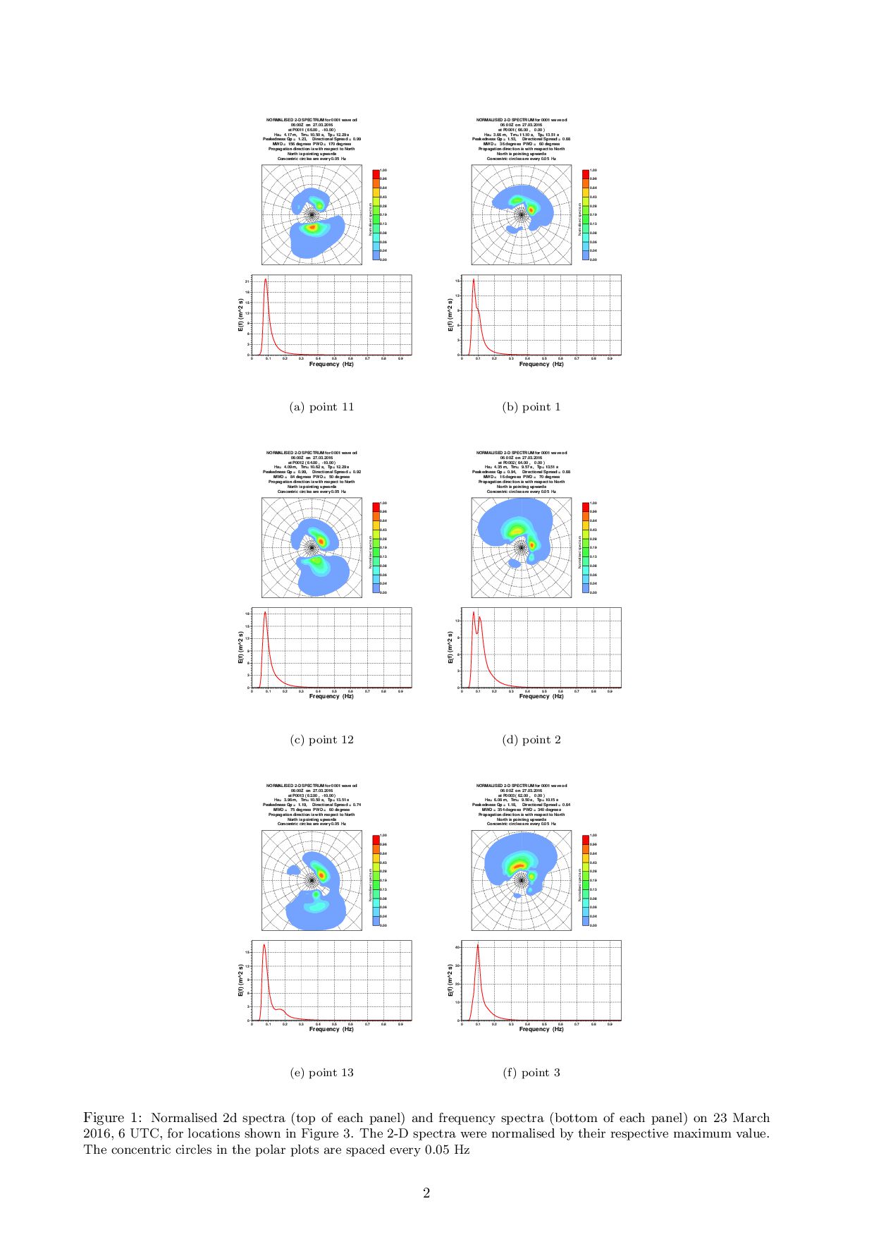
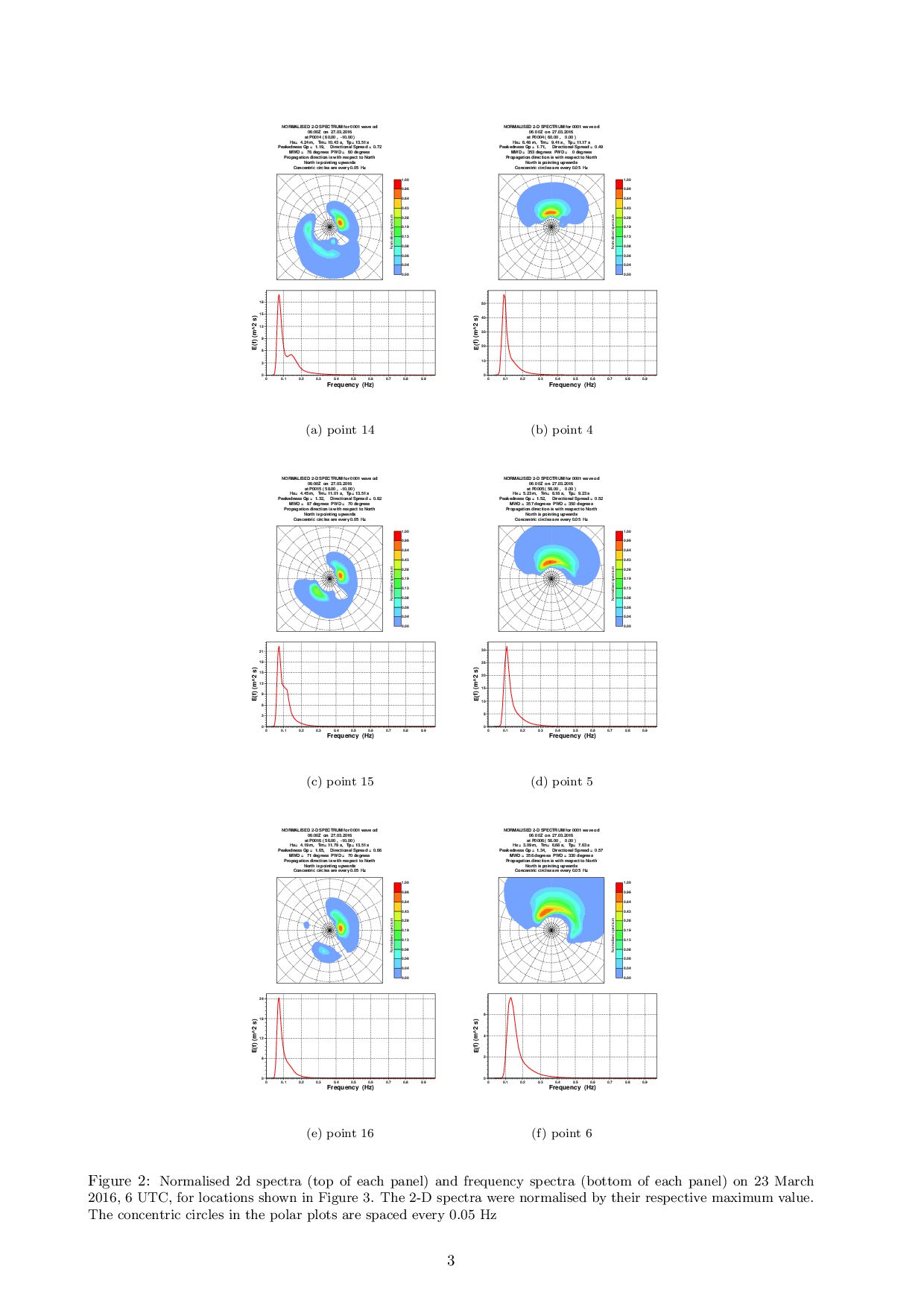
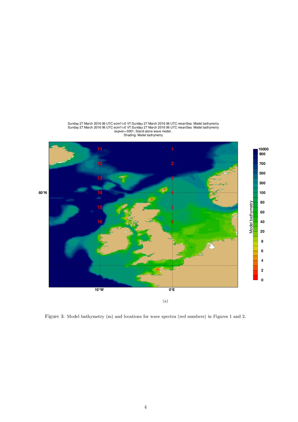
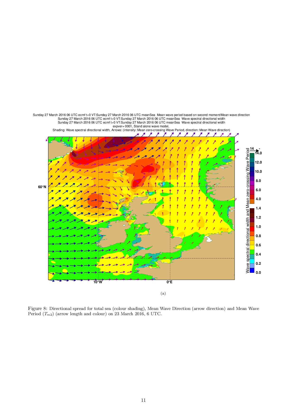
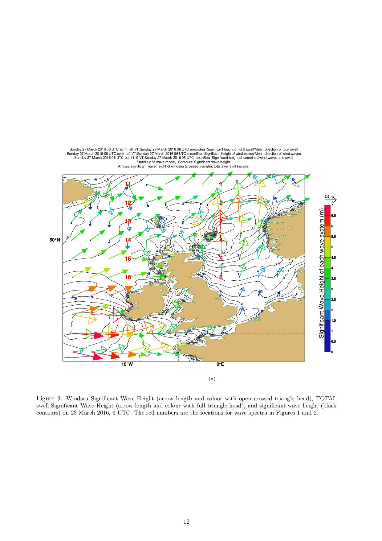
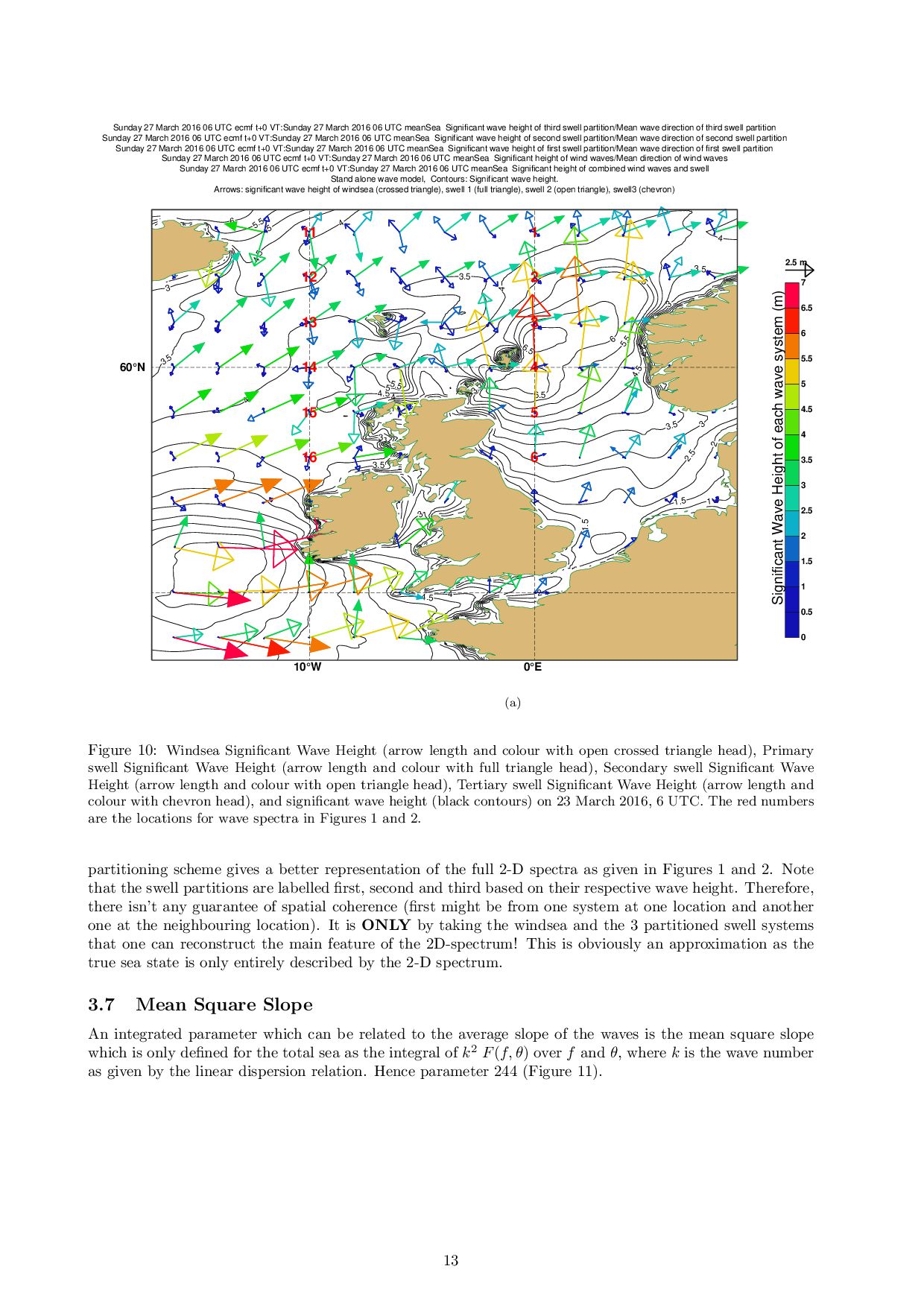
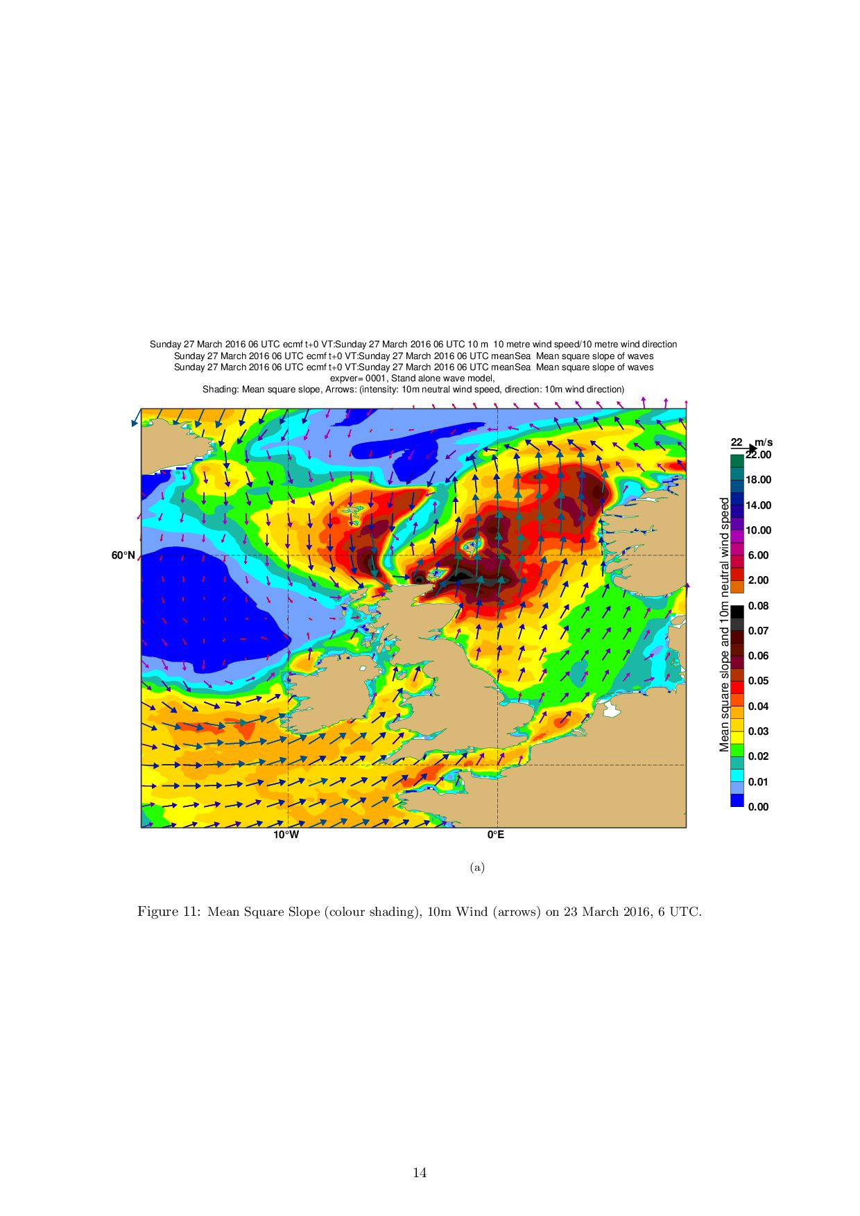
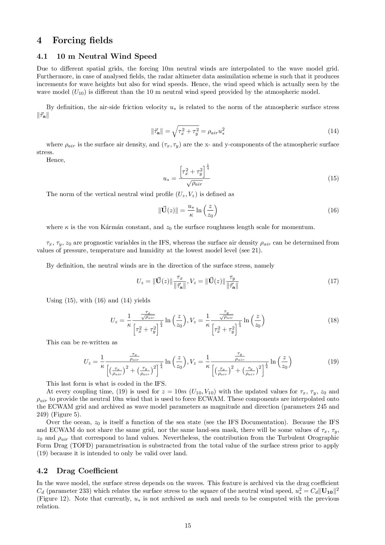
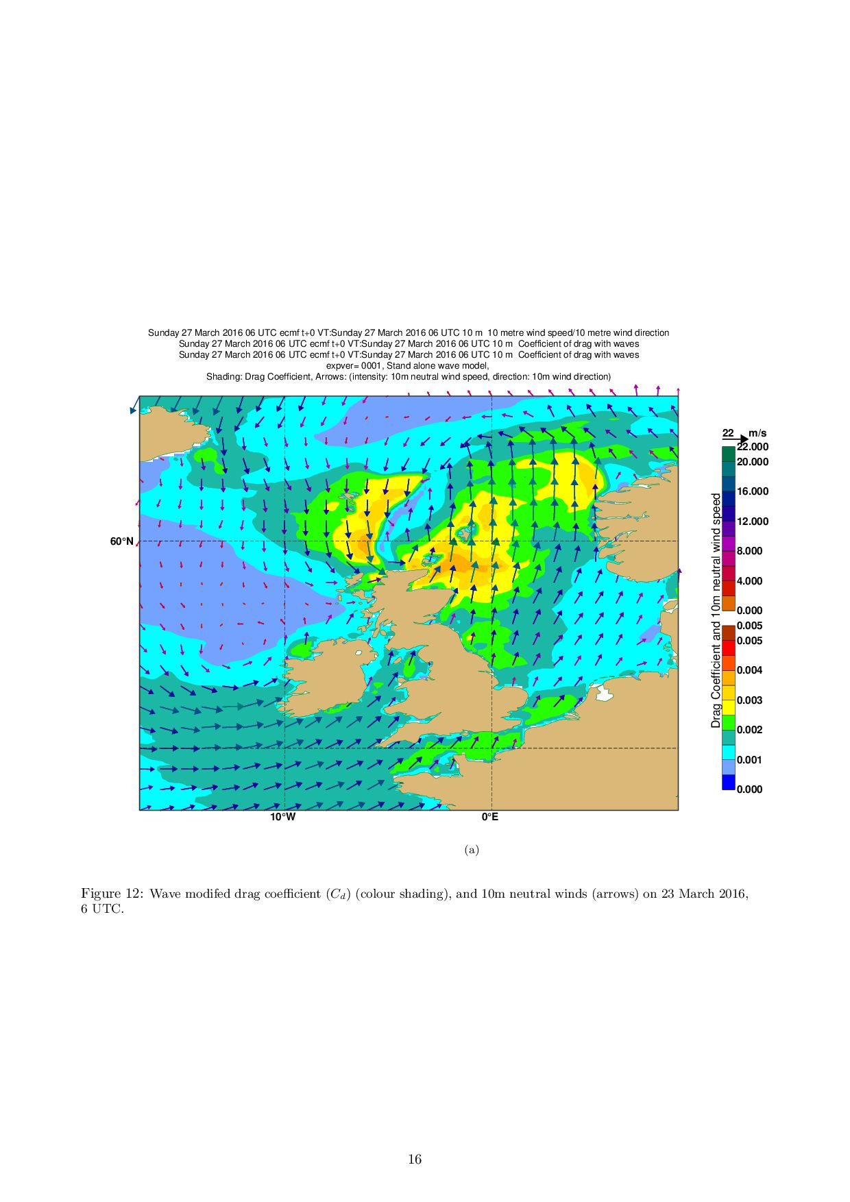
10. 3.4 Mean Wave Direction By weighting F(f, θ), one can also define a mean direction θ as θ = atan(SF/CF) (9) where SF is the integral of sin(θ) F(f, θ) over f and θ and CF is the integral of cos(θ) F(f, θ) over f and θ. Hence the definition of parameters 230, 235, 238, and the partitioned 122, 125, 128. Note that in grib 1, the direction parameters are encoded using the meteorological convention (0 means from North, 90 from East). 3.5 Wave Directional Spread Information on the directional distribution of the different wave components can be obtained from the mean directional spread σθ given by σθ = 2(1 − M1 ) (10) where For total sea: M1 = I1 /E0 (11) I1 is the integral of cos(θ− θ (f)) F(f, θ) over f and θ, where θ (f) is the mean direction at frequency f: θ (f) = atan(sf(f)/cf(f)) (12) with sf(f) the integral of sin(θ) F(f, θ) over θ only and cf(f) is the integral of cos(θ) F(f, θ) over θ only. Hence the definition of parameter 222. For wind waves and swell: M1 = Ip /E(fp ) (13) Ip is the integral of cos(θ − θ (fp )) F(fp , θ) over θ only, fp is the frequency at the spectral peak and θ (fp ) is given by (12), where F(fp , θ) is still split in all calculations using (1) (including in E(fp )). Hence the definition of parameters 225, 228. Note: As defined by (10), the mean directional spread σθ takes values between 0 and √ 2, where 0 corresponds to a uni-directional spectrum (M1 = 1) and √ 2 to a uniform spectrum (M1 = 0). Figure 8 shows the directional spread for total sea, mean wave direction and zero-crossing mean wave period corresponding to the synoptic situation as shown in Figure 5. The plot highlights areas where the sea state is composed of different wave systems as shown in Figures 1 and 2. 3.6 Spectral partitioning Traditionally, the wave model has separated the 2D-spectrum into a windsea and a total swell part (see above). Figure 9 shows the windsea and total swell significant wave height and mean wave direction corre- sponding to the synoptic situation as shown in Figure 5. However, in many instances, the swell part might actually be made up of different swell systems. Comparing the wave spectra in Figures 1 and 2 with the simple decomposition shown in Figure 9, it is clear that for many locations, the total swell is made up of more that one distinct wave system. We have adapted and optimised the spectral partitioning algorithm of Hanson and Phillips (2001) to decompose the SWELL spectrum into swell systems. It uses the fact that the spectra are model spectra for which a high frequency tail has been imposed and it excludes from the search the windsea part (the original partitioning method decomposes the full two-dimensional spectrum). The three most energetic swell systems are retained (for most cases, up to 3 swell partitions was found to be enough) and the spectral variance contained in the other partitions (if any) is redistributed proportionally to the spectral variance of the three selected partitions. Because it is only the swell spectrum that is partitioned, some spectral components can end up being unassigned to any swell partitions, their variance should be assigned to the windsea if they are in the wind directional sector, but it is currently NOT done because the old definition of the windsea and the total swell was not modified, otherwise they are redistributed proportionally to the spectral variance of the three selected partitions. Based on the partitioned spectrum, the corresponding significant wave height (4), mean wave direction (9), and mean frequency (5) are computed. So, by construct, the 2D-spectrum is decomposed into windsea (using the old defitinition) and up to three swell partitions, each described by significant wave height, mean wave period and mean direction. Figure 10 shows how the partitioning has decomposed the spectra. Compared to Figure 9, it can be seen that the new 10
11. 60°N 0°E 10°W Shading: Wave spectral directional width, Arrows: (intensity: Mean zero-crossing Wave Period, direction: Mean Wave direction) expver= 0001, Stand alone wave model, Sunday 27 March 2016 06 UTC ecmf t+0 VT:Sunday 27 March 2016 06 UTC meanSea Wave spectral directional width Sunday 27 March 2016 06 UTC ecmf t+0 VT:Sunday 27 March 2016 06 UTC meanSea Wave spectral directional width Sunday 27 March 2016 06 UTC ecmf t+0 VT:Sunday 27 March 2016 06 UTC meanSea Mean wave period based on second moment/Mean wave direction Wave spectral directional width and Mean zero-crossing Wave Period 0.0 0.2 0.4 0.6 0.8 1.0 1.2 1.4 4.0 6.0 8.0 10.0 12.0 14.0 14 - (a) Figure 8: Directional spread for total sea (colour shading), Mean Wave Direction (arrow direction) and Mean Wave Period (Tm2 ) (arrow length and colour) on 23 March 2016, 6 UTC. 11
12. 2 2 2 4 4 4 4 4 4 6 6 2.5 2.5 4.5 4.5 4.5 4.5 6.5 6.5 1 3 3 3 3 3 5 5 5 1.5 1.5 3.5 3.5 3.5 3.5 3.5 3.5 5.5 5.5 5.5 1 2 3 4 5 6 11 12 13 14 15 16 60°N 0°E 10°W Arrows: significant wave height of windsea (crossed triangle), total swell (full triangle) Stand alone wave model, Contours: Significant wave height. Sunday 27 March 2016 06 UTC ecmf t+0 VT:Sunday 27 March 2016 06 UTC meanSea Significant height of combined wind waves and swell Sunday 27 March 2016 06 UTC ecmf t+0 VT:Sunday 27 March 2016 06 UTC meanSea Significant height of wind waves/Mean direction of wind waves Sunday 27 March 2016 06 UTC ecmf t+0 VT:Sunday 27 March 2016 06 UTC meanSea Significant height of total swell/Mean direction of total swell Significant Wave Height of each wave system (m) 0 0.5 1 1.5 2 2.5 3 3.5 4 4.5 5 5.5 6 6.5 7 2.5 m (a) Figure 9: Windsea Significant Wave Height (arrow length and colour with open crossed triangle head), TOTAL swell Significant Wave Height (arrow length and colour with full triangle head), and significant wave height (black contours) on 23 March 2016, 6 UTC. The red numbers are the locations for wave spectra in Figures 1 and 2. 12
13. 2 2 2 4 4 4 4 4 4 6 6 2.5 2.5 4.5 4.5 4.5 4.5 6.5 6.5 1 3 3 3 3 3 5 5 5 1.5 1.5 3.5 3.5 3.5 3.5 3.5 3.5 5.5 5.5 5.5 1 2 3 4 5 6 11 12 13 14 15 16 60°N 0°E 10°W Arrows: significant wave height of windsea (crossed triangle), swell 1 (full triangle), swell 2 (open triangle), swell3 (chevron) Stand alone wave model, Contours: Significant wave height. Sunday 27 March 2016 06 UTC ecmf t+0 VT:Sunday 27 March 2016 06 UTC meanSea Significant height of combined wind waves and swell Sunday 27 March 2016 06 UTC ecmf t+0 VT:Sunday 27 March 2016 06 UTC meanSea Significant height of wind waves/Mean direction of wind waves Sunday 27 March 2016 06 UTC ecmf t+0 VT:Sunday 27 March 2016 06 UTC meanSea Significant wave height of first swell partition/Mean wave direction of first swell partition Sunday 27 March 2016 06 UTC ecmf t+0 VT:Sunday 27 March 2016 06 UTC meanSea Significant wave height of second swell partition/Mean wave direction of second swell partition Sunday 27 March 2016 06 UTC ecmf t+0 VT:Sunday 27 March 2016 06 UTC meanSea Significant wave height of third swell partition/Mean wave direction of third swell partition Significant Wave Height of each wave system (m) 0 0.5 1 1.5 2 2.5 3 3.5 4 4.5 5 5.5 6 6.5 7 2.5 m (a) Figure 10: Windsea Significant Wave Height (arrow length and colour with open crossed triangle head), Primary swell Significant Wave Height (arrow length and colour with full triangle head), Secondary swell Significant Wave Height (arrow length and colour with open triangle head), Tertiary swell Significant Wave Height (arrow length and colour with chevron head), and significant wave height (black contours) on 23 March 2016, 6 UTC. The red numbers are the locations for wave spectra in Figures 1 and 2. partitioning scheme gives a better representation of the full 2-D spectra as given in Figures 1 and 2. Note that the swell partitions are labelled first, second and third based on their respective wave height. Therefore, there isn’t any guarantee of spatial coherence (first might be from one system at one location and another one at the neighbouring location). It is ONLY by taking the windsea and the 3 partitioned swell systems that one can reconstruct the main feature of the 2D-spectrum! This is obviously an approximation as the true sea state is only entirely described by the 2-D spectrum. 3.7 Mean Square Slope An integrated parameter which can be related to the average slope of the waves is the mean square slope which is only defined for the total sea as the integral of k2 F(f, θ) over f and θ, where k is the wave number as given by the linear dispersion relation. Hence parameter 244 (Figure 11). 13
14. 60°N 0°E 10°W Shading: Mean square slope, Arrows: (intensity: 10m neutral wind speed, direction: 10m wind direction) expver= 0001, Stand alone wave model, Sunday 27 March 2016 06 UTC ecmf t+0 VT:Sunday 27 March 2016 06 UTC meanSea Mean square slope of waves Sunday 27 March 2016 06 UTC ecmf t+0 VT:Sunday 27 March 2016 06 UTC meanSea Mean square slope of waves Sunday 27 March 2016 06 UTC ecmf t+0 VT:Sunday 27 March 2016 06 UTC 10 m 10 metre wind speed/10 metre wind direction Mean square slope and 10m neutral wind speed 0.00 0.01 0.02 0.03 0.04 0.05 0.06 0.07 0.08 2.00 6.00 10.00 14.00 18.00 22.00 22 m/s (a) Figure 11: Mean Square Slope (colour shading), 10m Wind (arrows) on 23 March 2016, 6 UTC. 14
15. 4 Forcing fields 4.1 10 m Neutral Wind Speed Due to different spatial grids, the forcing 10m neutral winds are interpolated to the wave model grid. Furthermore, in case of analysed fields, the radar altimeter data assimilation scheme is such that it produces increments for wave heights but also for wind speeds. Hence, the wind speed which is actually seen by the wave model (U10 ) is different than the 10 m neutral wind speed provided by the atmospheric model. By definition, the air-side friction velocity u∗ is related to the norm of the atmospheric surface stress τa τa = τ2 x + τ2 y = ρair u2 ∗ (14) where ρair is the surface air density, and (τx , τy ) are the x- and y-components of the atmospheric surface stress. Hence, u∗ = τ2 x + τ2 y 1 4 √ ρair (15) The norm of the vertical neutral wind profile (Uz , Vz ) is defined as U(z) = u∗ κ ln z z0 (16) where κ is the von K´ arm´ an constant, and z0 the surface roughness length scale for momentum. τx , τy , z0 are prognostic variables in the IFS, whereas the surface air density ρair can be determined from values of pressure, temperature and humidity at the lowest model level (see 21). By definition, the neutral winds are in the direction of the surface stress, namely Uz = U(z) τx τa , Vz = U(z) τy τa (17) Using (15), with (16) and (14) yields Uz = 1 κ τx √ ρair τ2 x + τ2 y 1 4 ln z z0 , Vz = 1 κ τy √ ρair τ2 x + τ2 y 1 4 ln z z0 (18) This can be re-written as Uz = 1 κ τx ρair τx ρair 2 + τy ρair 2 1 4 ln z z0 , Vz = 1 κ τy ρair τx ρair 2 + τy ρair 2 1 4 ln z z0 (19) This last form is what is coded in the IFS. At every coupling time, (19) is used for z = 10m (U10 , V10 ) with the updated values for τx , τy , z0 and ρair to provide the neutral 10m wind that is used to force ECWAM. These components are interpolated onto the ECWAM grid and archived as wave model parameters as magnitude and direction (parameters 245 and 249) (Figure 5). Over the ocean, z0 is itself a function of the sea state (see the IFS Documentation). Because the IFS and ECWAM do not share the same grid, nor the same land-sea mask, there will be some values of τx , τy , z0 and ρair that correspond to land values. Nevertheless, the contribution from the Turbulent Orographic Form Drag (TOFD) parametrisation is substracted from the total value of the surface stress prior to apply (19) because it is intended to only be valid over land. 4.2 Drag Coefficient In the wave model, the surface stress depends on the waves. This feature is archived via the drag coefficient Cd (parameter 233) which relates the surface stress to the square of the neutral wind speed, u2 ∗ = Cd U10 2 (Figure 12). Note that currently, u∗ is not archived as such and needs to be computed with the previous relation. 15
16. 60°N 0°E 10°W Shading: Drag Coefficient, Arrows: (intensity: 10m neutral wind speed, direction: 10m wind direction) expver= 0001, Stand alone wave model, Sunday 27 March 2016 06 UTC ecmf t+0 VT:Sunday 27 March 2016 06 UTC 10 m Coefficient of drag with waves Sunday 27 March 2016 06 UTC ecmf t+0 VT:Sunday 27 March 2016 06 UTC 10 m Coefficient of drag with waves Sunday 27 March 2016 06 UTC ecmf t+0 VT:Sunday 27 March 2016 06 UTC 10 m 10 metre wind speed/10 metre wind direction Drag Coefficient and 10m neutral wind speed 0.000 0.001 0.002 0.003 0.004 0.005 0.005 0.000 4.000 8.000 12.000 16.000 20.000 22.000 22 m/s (a) Figure 12: Wave modifed drag coefficient (Cd ) (colour shading), and 10m neutral winds (arrows) on 23 March 2016, 6 UTC. 16
17. 4.3 Free convective velocity scale and air density Strickly speaking the free convective velocity (w∗ ) (parameter 208) and the air density (ρair ) (parameter 209) are not wave model parameters, they are part of the atmospheric forcing. Nevertheless, they are archived on the same model grid as the wave model, and are only available over the oceans, as defined by the wave model land/sea mask. The free convection velocity scale w∗ is used to parameterise the impact of wind gustiness on the wave growth which is also propotional to the ratio of air density to water density (currently assumed constant). The free convection velocity scale w∗ is computed using w∗ = u∗ 1 κ zi −L 1/3 for L < 0 and w∗ = 0 for L >= 0 (20) where u∗ is the friction velocity (u2 ∗ = τa ρair ), κ is the von K´ arm´ an constant, zi is the height of the lowest inversion, L is the Monin-Obukhov length. The quantity zi /L, which is a measure for the atmospheric stability, is readily available from the atmospheric model, and the surface air density ρair is given by ρair = P RTv (21) where P is the atmospheric pressure, R 287.04 J kg−1 K−1 is a constant defined as R = R+ /ma , with R+ the universal gas constant (R+ 8314.36 J kmol−1 K−1) and ma is the molecular weight of the dry air ( 28.966 kg kmol−1), and Tv is the virtual temperature. The virtual temperature can be related to the actual air temperature, T, and the specific humidity, q, by: Tv (1 + 0.6078q)T. To avoid using diagnostic variables, the pressure, the temperature and humidity at the lowest model level are now used. Figure 13 shows a combined map of the different fields that make up the forcing to the ECMWF wave model (U10 , ρair , w∗ ) . 17
18. 0.8 0.8 0.8 0.8 0.8 0.8 0.8 0.8 0.2 0.2 1 1 1 1 1 1 0.4 0.4 1.2 1.2 1.2 0.6 0.6 0.6 0.6 0.6 0.6 1.4 1.4 60°N 0°E 10°W Shading: Air density, Countours : Free convective velocity, Arrows: (intensity: 10m neutral wind speed, direction: 10m wind direction) expver= 0001, Coupled wave model, Sunday 27 March 2016 06 UTC ecmf t+0 VT:Sunday 27 March 2016 06 UTC meanSea Air density over the oceans Sunday 27 March 2016 06 UTC ecmf t+0 VT:Sunday 27 March 2016 06 UTC meanSea Air density over the oceans Sunday 27 March 2016 06 UTC ecmf t+0 VT:Sunday 27 March 2016 06 UTC 10 m 10 metre wind speed/10 metre wind direction Sunday 27 March 2016 06 UTC ecmf t+0 VT:Sunday 27 March 2016 06 UTC meanSea Free convective velocity over the oceans Air density and 10m neutral wind speed 1.10 1.15 1.20 1.25 1.30 1.50 4.50 7.50 10.50 13.50 16.50 19.50 22.50 24.00 24 m/s (a) Figure 13: Surface air density (ρair ) (colour shading), free convection velocity scale (w∗ ) (black contours), and 10m neutral winds (arrows) on 23 March 2016, 6 UTC. 18
19. 60°N 0°E 10°W Shading: Ratio of Surface Stokes Drift to 10m Wind Speed(%), Arrows: (intensity: Surface Stokes Drift ) expver= 0001, Stand alone wave model, Sunday 27 March 2016 06 UTC ecmf t+0 VT:Sunday 27 March 2016 06 UTC meanSea U-component stokes drift Sunday 27 March 2016 06 UTC ecmf t+0 VT:Sunday 27 March 2016 06 UTC meanSea U-component stokes drift Sunday 27 March 2016 06 UTC ecmf t+0 VT:Sunday 27 March 2016 06 UTC meanSea U-component stokes drift/V-component stokes drift Ratio of Surface Stokes Drift to 10m Wind Speed(%) and Surface Stokes Drift 0.0 1.0 2.0 3.0 4.0 5.0 6.0 0.1 0.3 0.5 0.7 0.9 1.1 1.2 1.2 m/s (a) Figure 14: Ratio (in percentage) of the surface Stokes drift magnitude to the 10m wind speed (colour shading), surface Stokes drift (arrow length and colour) on 23 March 2016, 6 UTC. 5 Interaction with the ocean circulation 5.1 Stokes drift The surface Stokes drift ust is defined by the following integral expression ust = dfdθ 2gk ω tanh(2kD) kF(f, θ) (22) The integration is performed over all frequencies and directions. In the high-frequency range the usual Phillips spectral shape is used where the Phillips parameter is determined by the spectral level at the last frequency bin, while it is tacitly assumed that these frequencies are so high that shallow water effects are unimportant. This defines parameters 215 and 216. Figure 14 shows the ratio (in percentage) of the surface Stokes drift magnitude to the 10m wind speed (colour shading) and the actual surface Stokes drift (colour arrows) corresponding to the synoptic situation as shown in Figure 5 for wind. This ratio shows that the surface Stokes drift cannot easily be represented as a fixed ratio of the 10m wind speed. 5.2 Momentum and energy flux into ocean In order to be able to give a realistic representation of the mixing processes in the surface layer of the ocean, a reliable estimate of energy and momentum fluxes to the ocean column is required. As energy and momentum flux depend on the spectral shape, the solution of the energy balance equation is required. It 19
20. reads ∂ ∂t F + ∂ ∂x · (vg F) = Sin + Snl + Sdiss + Sbot , (23) where F = F(ω, θ) is the two-dimensional wave spectrum which gives the energy distribution of the ocean waves over angular frequency ω and propagation direction θ. Furthermore, vg is the group velocity and on the right hand side there are four source terms. The first one, Sin describes the generation of ocean waves by wind and therefore represents the momentum and energy transfer from air to ocean waves. The third and fourth term describe the dissipation of waves by processes such as white-capping, large scale breaking eddy-induced damping and bottom friction, while the second term denotes nonlinear transfer by resonant four-wave interactions. The nonlinear transfer conserves total energy and momentum and is important in shaping the wave spectrum and in the spectrum down-shift towards lower frequencies. Let us first define the momentum and energy flux. The total wave momentum M depends on the variance spectrum F(ω, θ) and is defined as M = ρw g 2π 0 ∞ 0 dωdθ k ω F(ω, θ), (24) where ρw is the water density and g the acceleration due to gravity. The momentum fluxes to and from the wave field are given by the rate of change in time of wave momentum, and one may distinguish different momentum fluxes depending on the different physical processes. For example, making use of the energy balance equation (23) the wave-induced stress is given by τin = ρw g 2π 0 ∞ 0 dωdθ k ω Sin (ω, θ), (25) while the dissipation stress is given by τdiss = ρw g 2π 0 ∞ 0 dωdθ k ω Sdiss (ω, θ), (26) Similarly, the energy flux from wind to waves is defined by Φin = ρw g 2π 0 ∞ 0 dωdθ Sin (ω, θ), (27) and the energy flux from waves to ocean, Φdiss , is given by Φdiss = ρw g 2π 0 ∞ 0 dωdθ Sdiss (ω, θ). (28) It is important to note that while the momentum fluxes are mainly determined by the high-frequency part of the wave spectrum, the energy flux is to some extent also determined by the low-frequency waves. The prognostic frequency range is limited by practical considerations such as restrictions on computation time, but also by the consideration that the high-frequency part of the dissipation source function is not well-known. In the ECMWF wave model the high-frequency limit ωc = 2πfc is set as fc = min{fmax , 2.5 f windsea } (29) Thus, the high-frequency extent of the prognostic region is scaled by the mean frequency f windsea of the local windsea. A dynamic high-frequency cut-off, fc , rather than a fixed cut-off at fmax , corresponding to the last discretised frequency, is necessary to avoid excessive disparities in the response time scales within the spectrum. In the diagnostic range, ω > ωc , the wave spectrum is given by Phillips’ ω−5 power law. In the diagnostic range it is assumed that there is a balance between input and dissipation. In practice this means that all energy and momentum going into the high-frequency range of the spectrum is dissipated, and is therefore directly transferred to the ocean column. 2π 0 ∞ ωc dωdθ k ω (Sin + Sdiss + SNL ) = 0, (30) and 20
21. 2π 0 ∞ ωc dωdθ (Sin + Sdiss + SNL ) = 0, (31) The momentum flux to the ocean column, denoted by τoc , is the sum of the flux transferred by turbulence across the air-sea interface which was not used to generate waves τa −τin and the momentum flux transferred by the ocean waves due to wave breaking τdiss . As a consequence, τoc = τa − τin − τdiss . Utilizing the assumed balance at the high-frequencies (30) and the conservation of momentum for SNL when integrated over all frequencies and directions, one finds τoc = τa − ρw g 2π 0 ωc 0 dωdθ k ω (Sin + Sdiss + SNL ) , (32) where τa is the atmospheric stress, whose magnitude is given by τa = ρair u2 ∗ , with u∗ the air side friction velocity. Ignoring the direct energy flux from air to ocean currents, because it is small, the energy flux to the ocean, denoted by Φoc , is therefore given by −Φdiss . Utilizing the assumed high-frequency balance (31) and the conservation of energy when SNL is integrated over all frequencies and directions, one therefore obtains Φoc = ρw g 2π 0 ∞ ωc dωdθ Sin − ρw g 2π 0 ωc 0 dωdθ (Sdiss + SNL ) , (33) The high frequency (ω > ωc ) contribution to the energy flux Φochf = ρw g 2π 0 ∞ ωc dωdθ Sin (34) is parameterised following the same approach as for the kinematic wave induced stress (for more details refer to the IFS documentation part VII) Φochf = ρa (2π)4f5 c g u∗ 2 2π 0 dθ F(fc , θ)[max (cos(θ − φ), 0)]2 βm κ2 ∞ ωc dω ω2 µhf ln4(µhf ), (35) In (35), the integral over directions can be evaluated using the prognostic part of the spectrum, whereas the second integral is only function of u∗ and the Charnock parameter. It can therfore be tabulated beforehand. Note that the integration is bounded because µhf <= 1 PHIOCHF = βm κ2 z0 g 1 Yc dY Y 2 µhf ln4(µhf ), Yc = max ωc , x0 g u∗ z0 g (36) where for typical values of the Charnock parameter, x0 ∼ 0.05. The archived energy fluxes are normalized by the product of the air density ρair and the cube of the friction velocity in the air (u∗ ). Hence the normalized energy flux into waves (parameter 211) is obtained from (27) divided by ρair u3 ∗ . Similarly the normalized energy flux into ocean (parameter 212) is obtained from normalizing (33). The normalized stress into ocean (parameter 214) is derived from (32) by dividing it with the atmospheric stress τa = ρair u2 ∗ . Figure 15 shows both dimensional energy and momentum fluxes into the ocean. 21
22. 60°N 0°E 10°W Shading: Turbulent Energy flux into the ocean, Arrows: (intensity: Momentum Flux into the Ocean, direction: 10m Wind Direction) expver= 0001, Stand alone wave model, Sunday 27 March 2016 06 UTC ecmf t+0 VT:Sunday 27 March 2016 06 UTC meanSea Normalized energy flux into ocean Sunday 27 March 2016 06 UTC ecmf t+0 VT:Sunday 27 March 2016 06 UTC meanSea Normalized energy flux into ocean Sunday 27 March 2016 06 UTC ecmf t+0 VT:Sunday 27 March 2016 06 UTC meanSea/heightAboveGround Normalized stress into ocean/10 metre wind direction Turbulent Energy flux into the ocean and Momentum Flux into the Ocean 0.0 2.0 4.0 6.0 8.0 10.0 11.0 0.0 0.4 0.8 1.2 1.6 1.6 N/m^2 (a) Figure 15: Wave energy flux into the ocean (colour shading), and momentum flux into the ocean (arrows) on 23 March 2016, 6 UTC. 22
23. 6 Freak wave parameters The parameters that have been described so far all provide information on the average properties of the sea state. In recent years, there has been a considerable effort to understand extreme events such as freak waves. An individual wave is regarded as a freak wave when its height is larger than twice the significant wave height. Clearly, in order to be able to describe such extreme events, knowledge on the statistical properties of the sea surface is required. Recent work has presented a general framework that relates the shape of the probability distribution function (pdf) of the surface elevation to the mean sea state as described by the two- dimensional frequency spectrum. Under normal circumstances, the surface elevation pdf has approximately a Gaussian shape, but in the exceptional circumstances that the waves are sufficiently nonlinear and that the wave spectrum is narrow in both frequency and direction considerable deviations from Normality may occur, signalling increased probability for freak waves. The deviations from Normality are measured in terms of the kurtosis C4 (parameter 252) of the surface elevation pdf. The determination of this parameter from the wave spectrum is described in Chapter 8 of part VII of the IFS documentation, and it is shown that in the narrow-band approximation the kurtosis depends on the Benjamin-Feir Index BFI and the directional width δω at the peak of the wave spectrum with some correction for shallow water effects. C4 = Cdyn 4 + κ4 8 . (37) where κ4 = κ40 + κ04 + 2κ22 . The κ’s refer to certain fourth-order cumulants of the joint pdf of the surface elevation and its Hilbert transform (?). κ40 = 18 ; κ04 = 0.; κ22 = κ40 6 = 3 with the integral steepness parameter, = k0 √ m0 , k0 the peak wave number, m0 the zero moment of the spectrum. and, Cdyn 4 = 1 1 + 7 2 δθ δω 2 × π 3 √ 3 −BFI2 × vg c0 2 gXnl kω0 ω0 , (38) where the relevant symbols are defined in capter 8 of the IFS documentation and the Benjamin-Feir Index BFI is given by BFI = √ 2 δω . (39) Note that the archived parameter (253) is the square of BFI. The Benjamin-Feir Index is the ratio of the integral wave steepness and δω the relative width of the frequency. Initially the relative width of the frequency spectrum was solely estimated by using Goda’s peakedness factor Qp (parameter 254) defined as Qp = 2 m2 0 dω ωE2(ω) (40) with E(ω) the angular frequency spectrum and the integration domain D consists of all frequencies for which E(ω) > 0.4 E(ωp ), with ωp the peak angular frequency. The advantage of this integral measure is that, because of its dependence on the square of the frequency spectrum, peaks in the spectrum are emphasized. Howver, from CY33R1 onwards, a sharper estimate of the width in frequency and direction is obtained from a two-dimensional parabolic fit around the peak of the spectrum. This procedure then also gives a more accurate estimation of the peak period (parameter 231). In the operational model, the kurtosis C4 is restricted to the range −0.33 < C4 < 1. Since CY40R3, the skewness of the pdf of the surface elevation C3 was introduced (parameter 207). This is in particular relevant for the contribution of bound waves to the deviations of statistics from Normality, as bound waves give rise to a considerable skewness. On the other hand, it should be noted that the skewness 23
24. of free waves is very small and therefore for really extreme events the skewness correction to the wave height pdf is not so important. However, on average, the bound waves will determine the statistics of waves and, therefore, in order to have an accurate desciption of the average conditions as well the skewness effect needs to be included. C3 = κ2 3 72 , (41) where κ2 3 = 5(k2 30 + κ2 03 ) + 9(κ2 21 + κ2 12 ) + 6(κ30 κ12 + κ03 κ21 ) The κ’s refer to certain third-order cumulants of the joint pdf of the surface elevation and its Hilbert transform (?). κ30 = 3 ; κ03 = 0.; κ12 = 0.; κ21 = κ30 3 = Finally, these deviations form Normality can be used to come up with an expression for the expectation value of the maximum wave height Hmax (parameter 218). Hmax = z Hs , (42) with Hs the significant wave height (4) where z = ˆ z0 + 1 4 √ ˆ z0 γ + log 1 + ˆ αC4 + ˆ βC2 3 , (43) with ˆ z0 = 1 2 log N and γ = 0.5772 is Euler’s constant where ˆ α = 2ˆ z0 (ˆ z0 − 1) + (1 − 2ˆ z0 )G1 + 1 2 G2 and ˆ β = ˆ z0 (4ˆ z2 0 − 12ˆ z0 + 6) − (6ˆ z2 0 − 12ˆ z0 + 3)G1 + 3(ˆ z0 − 1)G2 − 1 2 G3 , It may be shown that G1 = Γ (1) = −γ, G2 = Γ (1) = γ2 + π2 6 , and G3 = Γ (1) = −2ζ(3) − γ3 − γπ2/2). Here, ζ(3) = 1.20206 is the Riemann zeta function with argument 3. Finally the number of independant wave groups N in the time series of length TL has to be determined N = 2hc √ 2π ν¯ ωTL . (44) with ¯ ω = m1 /m0 the mean angular frequency, while ν = (m0 m2 /m2 1 − 1)1/2 is the width of the frequency spectrum and the reference level hc = √ 2. It is clear that for operational applications a choice for the length of the timeseries (TL ) needs to be made. A duration of 20 minutes (TL =1200 sec.) was selected to roughly correspond to buoy acquisition time. Figure 16 shows the ratio of Hmax to Hs corresponding to the synoptic situation as shown in Figure 5. 7 Miscellaneous 7.1 Radar Altimeter Data These parameters are only for diagnostics carried out at ECMWF Even though altimeter data are processed observations and thus not as such wave model results, their processing has required some information from the model. Following a quality control procedure which discards all spurious data, the raw altimeter wave height data, which are available in a ±3 hours time window, is collocated with the closest model grid point. The 24
25. 60°N 0°E 10°W Shading: Ratio of Hmax to Hs , Arrows: (intensity: Significant Wave Height (Hs), direction: Mean Wave Direction) expver= 0001, Stand alone wave model, Sunday 27 March 2016 06 UTC ecmf t+0 VT:Sunday 27 March 2016 06 UTC meanSea Maximum individual wave height Sunday 27 March 2016 06 UTC ecmf t+0 VT:Sunday 27 March 2016 06 UTC meanSea Maximum individual wave height Sunday 27 March 2016 06 UTC ecmf t+0 VT:Sunday 27 March 2016 06 UTC meanSea Significant height of combined wind waves and swell/Mean wave direction Ratio of Hmax to Hs and Significant Wave Height (Hs) 1.4 1.5 1.7 1.9 2.1 2.3 1.0 3.0 5.0 7.0 9.0 9 m (a) Figure 16: Ratio of Hmax to Hs (colour shading), Significant Wave Height (Hs ) (arrow length and colour) on 23 March 2016, 6 UTC. 25
26. average value is computed for all grid points with at least two individual observations. The averaged data are then archived on the same grid as all wave model fields as parameter 246. Before these gridded altimeter wave heights are presented to the wave model assimilation scheme, cor- rections are performed which depend on the type of Altimeter instrument. For example, however because of a known underestimation of significant wave height by the ERS-2 satellite, which is due to the inherent non gaussian distribution of the sea surface elevation and the method how wave height is obtained from the waveform, a correction is derived from the model spectra which is applied to the altimeter data. Also data from the Altimeters on board of Envisat and Jason-1 are bias corrected. The correction is obtained from a comparison with buoy wave height data. The corrected data are used by the assimilation scheme and are archived as parameter 247. The altimeter range observation is also affected by the non gaussianity of the sea surface elevation. The correction is a fraction of the observed wave height, where the fraction depends on the nonlinearity of the sea surface. This number is also collocated with the wave model grid and archived as parameter 248. References J. Hanson and O. Phillips, 2001. Automated Analysis of Ocean Surface Directional Wave Spectra. J. Atmos. Oceanic. Technol.,18, 277–293. 26
27. Table 1: Archived parameters of the ECMWF wave forecasting system. Code Mars Field Units Figure Abbrev. 140120 SH10 Significant wave height of all waves with period larger than 10s m 140121 SWH1 Significant wave height of first swell partition m 140122 MWD1 Mean wave direction of first swell partition ◦ 140123 MWP1 Mean wave period of first swell partition s 140124 SWH2 Significant wave height of second swell partition m 140125 MWD2 Mean wave direction of second swell partition ◦ 140126 MWP2 Mean wave period of second swell partition s 140127 SWH3 Significant wave height of swell third partition m 140128 MWD3 Mean wave direction of swell third partition ◦ 140129 MWP3 Mean wave period of swell third partition s 140207 WSS Wave Spectral Skewness - 140208 WSTAR Free convective velocity scale over the oceans m/s 140209 RHOAO Air density over the oceans kg/m3 140211 PHIAW Normalized energy flux into waves - 140212 PHIOC Normalized energy flux into ocean - 140214 TAUOC Normalized stress into ocean - 140215 UST u-component of Stokes drift m/s 140216 VST v-component of Stokes drift m/s 140217 TPM Expected Period for Hmax s 140218 HMAX Expected Hmax over 3 hour period m 140219 DPTH Bathymetry as used by operational Wave Model m 140220 MP1 Mean wave period from 1st moment s 140221 MP2 Mean wave period from 2nd moment s 140222 WDW wave spectral directional width - 140223 P1WW Mean wave period from 1st moment of wind waves s 140224 P2WW Mean wave period from 2nd moment of wind waves s 140225 DWWW Wave spectral directional width of wind waves - 140226 P1PS Mean wave period from 1st moment of total swell s 140227 P2PS Mean wave period from 2nd moment of total swell s 140228 DWPS Wave spectral directional width of total swell - 140229 SWH Significant wave height m 140230 MWD Mean wave direction ◦ 140231 PP1D Peak period of 1-D spectra s 140232 MWP Mean wave period s 140233 CDWW Coefficient of drag with waves - 140234 SHWW Significant height of wind waves (windsea) m 140235 MDWW Mean direction of wind waves (windsea) ◦ 140236 MPWW Mean period of wind waves (windsea) s 140237 SHPS Significant height of total swell m 140238 MDPS Mean direction of total swell ◦ 140239 MPPS Mean period of total swell s 140244 MSQS Mean square slope - 140245 WIND 10 m neutral wind modified by wave model m/s 140246 AWH Gridded altimeter wave height m 140247 ACWH Gridded corrected altimeter wave height m 140248 ARRC Gridded altimeter range relative correction m 140249 DWI 10 m wind direction ◦ 140251 2DFD 2-D wave spectra m2s/rad 140252 WSK Kurtosis - 140253 BFI The square of the Benjamin-Feir Index - 140254 WSP Goda’s Peakedness parameter - 27