lecture_01_introduction_student_slides

Transcript

1. Introduction: Epidemiology III Lecture 1
2. THE SYLLABUS AND EXPECTATIONS 2
3. Instructor JEANINE GENKINGER, PHD, MHS • Email: jg3081@cumc.columbia.edu • Office: Mailman, Rm 712 (by appt only) 3
4. Prerequisites • Epidemiology II • Analysis of Categorical Data • Applications of Epidemiologic Research Methods • You are required to have taken these courses to register for this class 4
5. Resources/Texts COURSEWORKS SITE https://courseworks.columbia.edu/welcome/ RECOMMENDED TEXTS • Rothman K, Greenland S, Lash T. (2008) Modern Epidemiology (3rd edition). http://www.columbia.edu/cgi-bin/cul/resolve?clio8363805 • Hosmer DW, Lemeshow S (2013). Applied Logistic Regression (3rd edition). http://onlinelibrary.wiley.com/book/10.1002/9781118548387 • Hosmer DW, Lemeshow S (2008). Applied Survival Analysis. http://onlinelibrary.wiley.com/book/10.1002/9780470258019 SUPPLEMENTAL READING LIST (see last page of syllabus) • Contains recommended readings, additional textbook chapters and articles relevant to that week’s topic. PDFs of additional textbook and article readings will be provided on courseworks. SAS RESOURCE http://www.ats.ucla.edu/stat/sas/modules/ 5
6. Schedule • Tuesdays, September 3rd – December 10th – 1:00pm – 3:50pm – Lectures: Hammer, 301 (except 9/25: P&S Amp 7) – Labs: Hammer LL106, LL107, LL108A/B, LL109A/B, LL110 • One lecture and one recitation / computer lab per session • We expect you to attend all lectures and labs 6
7. Lecture Slides • Lecture slides will be posted on CourseWorks under Files & Resources – Slides will be saved as PDFs – They will be saved as one slide per page – However, you can print multiple slides per page by choosing this option on your computer (look for a “multiple pages” option in your print dialog box). • Slides will be posted the day before class 7
8. Lecture Recordings • Lectures will be taped with the slides but will not be automatically released on CourseWorks. • The taped classes will only be available on a case by case basis if you need to miss a class due to illness, disability, or any other need for audio reinforcement. • Please contact Richard Teran (rat2127@cumc.columbia.edu) to request regular access or to access for a specific class. We are happy to accommodate. 8
9. Pre-semester Assessment • Pre-semester assessment- 5% of your grade • Completion based • You will still receive a score for self- assessment • Please email/contact Dr. Genkinger and Richard Teran (rat2127) if you have not completed the assessment 9
10. Homeworks • Homework - 20% of your grade • Six homework assignments, each worth 4% • We drop the lowest grade • Homework due dates: • Released on CourseWorks • Due at the BEGINNING of class • No late homeworks will be accepted • If you know you will be late to class, send an email to your Lab TA and Dr. Genkinger • For all questions requiring calculations, use 4 decimal points during computations and round to two decimal points at the LAST step 10
11. Quizzes • Quizzes- 15% of your grade • 2 online take-home quizzes • 2 in class “pop” quizzes • Worth 5% each • We drop the lowest grade 11
12. Audience Response • Audience Response – 5% of your grade – To encourage participation, track your understanding of concepts and to give students an opportunity to submit real-time feedback on concepts that remain unclear following lecture. – Your Poll Everywhere account will be linked to your Courseworks gradebook, therefore, your account must be associated with your Columbia email. – The program can be accessed via the PollEverywhere app or through the following website: pollev.com/Jeaninegenki547. *if you have any issues, please email Richard at rat2127@cumc.Columbia.edu 12
13. Exams • Midterm – 25% of your grade –Tuesday, October 15th –In class closed-book exam • Final – 30% of your grade –In class closed-book exam, December 10th –Take-home open-book exam • Received: Tuesday, December 3rd • Due: Thursday, December 12th by 12:00pm • Final exams should be submitted in person. • You will NEED a PENCIL and a CALCULATOR (no cell phones or internet devices permitted) 13
14. Re-grading Policy • If students have questions about their grade on any assignment (homework, quiz, exam) they must bring it to Dr. Genkinger to discuss. After review, the student will be notified about the re-grade decision. 14
15. Teaching Assistants Teaching Assistant Email Adiba Ashrafi (Head TA) ai2337@cumc.columbia.edu Precious Esie pie2104@cumc.columbia.edu Diana Garofalo dcg2132@cumc.columbia.edu Shadiya Moss sm4248@cumc.columbia.edu John Pamplin jrp2166@cumc.columbia.edu Alex Perlmutter asp2183@cumc.columbia.edu Richard Teran rat2127@cumc.columbia.edu 15
16. Office Hours • Dr. Genkinger: by appointment (Room 712) 16 Teaching Assistant Office Hour Time Office Hour Location Shadiya Moss Mondays 11:00 AM – 12:00 PM ARB Room 739A Diana Garofalo Mondays 12:00 PM – 1:00 PM ARB Room 739A Precious Esie Tuesdays 11:00 AM – 12:00 PM ARB Room 1514 John Pamplin Tuesdays 12:00 PM – 1:00 PM ARB Room 1514 Alex Perlmutter TBD TBD Richard Teran TBD TBD Adiba Ashrafi TBD TBD
17. Emailing Questions • Please cc your assigned TA for your lab, Adiba Ashrafi (head TA) and Dr. Genkinger on all emails • We will respond to you within 24 hrs during the week and 48 hrs on the weekend 17
18. Honor Code 18 https://www.mailman.columbia.edu/sites/default/files/pdf/community-standards-and-conduct.pdf
19. Academic Integrity - Homework • Homework assignments: – You may discuss concepts and work through homework problems with classmates; however, the work you submit must be your own (e.g., in your own words, performing your own calculations, providing your own code and results). – It is in violation of the honor code to use answer keys from previous semesters to complete course assignments. Sharing of answer keys either directly or via internet upload is strictly prohibited in this class. **Anyone found to be in violation of these course procedures will be reported to OSA. 19
20. Academic Integrity - Quizzes • Take-home quizzes – Quizzes are open book/open notes, but must be completed independently. You cannot discuss the quiz or work with classmates to complete the quiz. You may only discuss the content of the quiz with classmates after the quiz due date (i.e. after all students have completed the quiz). **Anyone found to be in violation of these course procedures will be reported to OSA. 20
21. Academic Integrity – Final Exam • Take home Final exam: – Unlike homeworks, for the final exam you may not discuss concepts or work through exam questions with classmates – you must complete the final exam alone. If you have any clarification questions after release of the final exam you may direct them to the TAs and the professor. **Anyone found to be in violation of these course procedures will be reported to OSA. 21
22. Encouraging an Open and Inclusive Classroom Environment • The Department of Epidemiology is committed to creating an educational culture that encourages robust, open, and inclusive classroom environments. • Key to achieving this goal is to ensure that all students are included in the conversation and feel comfortable expressing themselves. • An inclusive classroom environment is undermined by microaggressions. 22
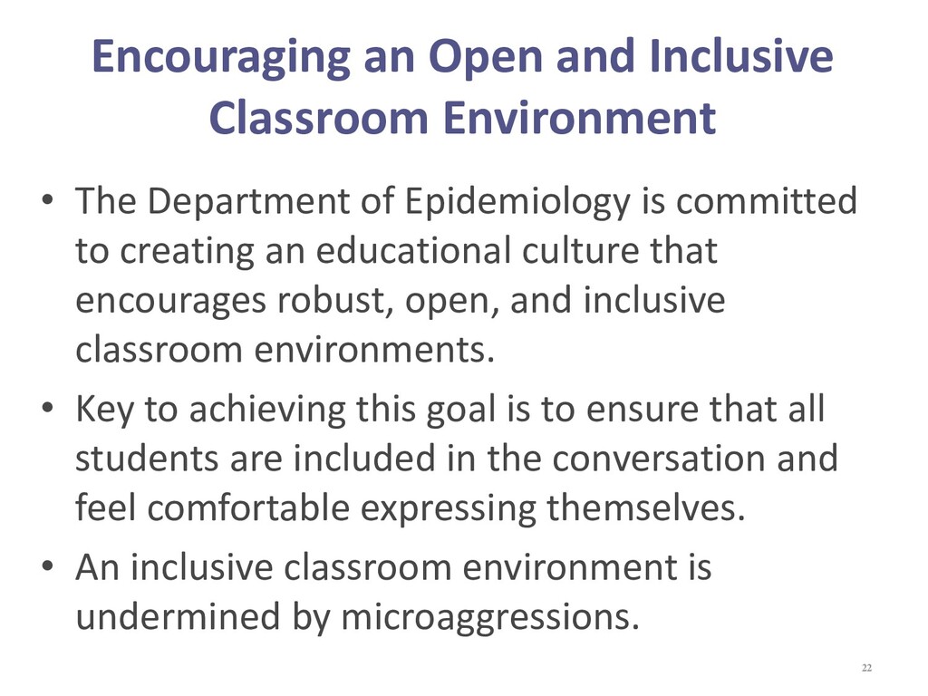
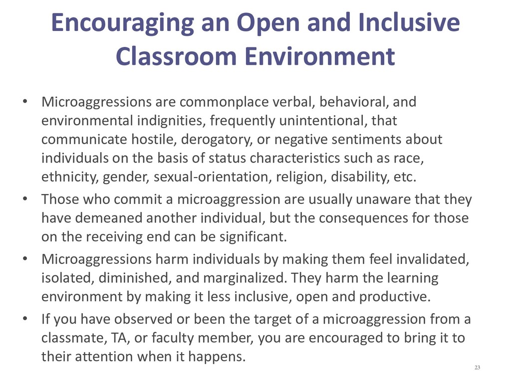
23. Encouraging an Open and Inclusive Classroom Environment • Microaggressions are commonplace verbal, behavioral, and environmental indignities, frequently unintentional, that communicate hostile, derogatory, or negative sentiments about individuals on the basis of status characteristics such as race, ethnicity, gender, sexual-orientation, religion, disability, etc. • Those who commit a microaggression are usually unaware that they have demeaned another individual, but the consequences for those on the receiving end can be significant. • Microaggressions harm individuals by making them feel invalidated, isolated, diminished, and marginalized. They harm the learning environment by making it less inclusive, open and productive. • If you have observed or been the target of a microaggression from a classmate, TA, or faculty member, you are encouraged to bring it to their attention when it happens. 23
24. Any questions?
25. Learning Objectives • Discuss how causal inference is central to the role of epidemiology in public health • Define and compare Measures of Effect and Measures of Association • Discuss Relationships Among Measures • Introduce the Multivariable Model 25
27. Causal Inference in Epidemiologic Research • We start with a research question: – Is circulating vitamin D concentration positively associated with CD4 count in an HIV+ population? – Does exposure to BPA increase your risk of obesity? – Does the HPV vaccine prevent oral cancers? • We want to answer does our exposure CAUSE our outcome…… 27
28. What is a cause? • Modern Epidemiology Definition: “an event, condition or characteristic that preceded the disease event and without which the disease event would not have occurred at all or would not have occurred until some later time” Rothman and Greenland (1998) 28
29. Causal inference in epidemiologic research 29 Theory of Causation Formulate a Testable Hypothesis Design and Conduct a Study Analyze Data Interpretation of Results
30. Causal inference in epidemiologic research 30 Theory of Causation • Potential Disease Determinant, i.e., risk factor exposure
31. Sufficient-Component Cause Model ’s Causal Pie 31 A B C E D Component Cause Rothman’s Causal Pie Each Causal Pie = “Causal Mechanism” = “Sufficient Cause” Component Cause: event or condition that plays a necessary role in the occurrence of some cases of disease
32. Sufficient-component cause model 32 A A A B B C C D E F F G H I J I II III • There are multiple mechanisms that cause any type of disease: 3 are illustrated here. • Each individual instance of disease will occur through a single sufficient cause. (A single pie) • What component is a necessary cause?
33. Attributes of the sufficient-component cause model • Blocking the action of one component cause prevents disease from occurring by that mechanism/pathway. • Therefore, it is unnecessary to know all of the component causes of a sufficient cause to prevent disease. 33 A E B C
34. Causal inference in epidemiologic research 34 Theory of Causation Formulate a Testable Hypothesis • Exposure to X will be related (or cause) a change in Y among entities in population P.
35. Causal inference in epidemiologic research 35 Theory of Causation Formulate a Testable Hypothesis Design and Conduct a Study • Randomized Trials, Cohort Studies, Case-Control Studies, Ecological Studies • Minimize Bias, Minimize Random Error, Collect Data on Confounding Variables
36. t + t today t - E D E D E D Cross sectional E D Retro Cohort Case-control Pros Cohort RCT (if E assigned) 36
37. Is there a hierarchy of study designs? Yes? – exchangeability/comparability – temporality No? – measurement validity – induction time – statistical power and efficiency 37
38. • Bias – Systematic error in the design and/or conduct of a study that results in an incorrect estimate of an exposure’s effect on the frequency of disease • Random Error – Result from measurement errors and sampling variability (by chance) • Confounding variables – Other “third” variables associated with both exposure and disease that distort the estimate of an exposure’s effect on the risk/rate of disease 38 Causal inference in epidemiologic research
39. Causal inference in epidemiologic research 39 Theory of Causation Formulate a Testable Hypothesis Design and Conduct a Study Analyze Data • Observe disease frequencies (risk, rate, prevalence) using comparisons, i.e. those exposed to causal factor vs. those unexposed to the casual factor • Calculate measures of association, i.e. RR and OR • Adjust for confounders
40. t + t today t - E D E D E D Cross sectional (prevalence odds) E D Retro Cohort (risk or rate) Case-control (odds) Pros Cohort/RCT (if E assigned) (risk or rate) 40
41. Causal inference in epidemiologic research 41 Theory of Causation Formulate a Testable Hypothesis Design and Conduct a Study Analyze Data Interpretation of Results • How strong is the association between exposure and disease? • Assess study validity: How precise is the estimate of effect? Is association due to bias and/or unadjusted confounding variables?
42. To answer our research question… Since we want to know about causal relationships and not just associations • First choice = what we want (but can’t have) – The counterfactual (or potential outcomes) 42
43. Counterfactuals 1. Disease experience of exposed cohort if, contrary to fact, they were unexposed, or 43
44. A B C F E D D Exposed cohort Exposed cohort if unexposed A B C F D D Note: A, B, C, and F are risk factors for disease Fact Contrary to fact 44
45. Counterfactuals 1. Disease experience of exposed cohort if, contrary to fact, they were unexposed, or 2. Disease experience of an unexposed cohort if, contrary to fact, they were exposed 45
46. A B C F E D D Exposed cohort Exposed cohort if unexposed A B C F D D Note: A, B, C, F, G and H are risk factors for disease Fact Contrary to fact 46 F G H B D D Unexposed cohort Unexposed cohort if exposed F G H B E D D
47. MEASURES OF EFFECT VS. ASSOCIATION 47
48. Measures of Effect • Same population  Counterfactual 48
49. A B C F E D D D1: Disease experience D2: Disease experience among exposed if remove exposure Absolute effects Relative effects A B C F D D Measure of Effect 49 Exposed cohort Exposed cohort if unexposed
50. From Table 4.1 in Rothman and Greenland Type Exp Unexp Exposed Cohort 1 1 1 Doomed p1 2 1 0 Exposure is causal p2 3 0 1 Exposure is preventive p3 4 0 0 Immune p4 50 1 = gets disease, 0 = does not get disease p = proportion of types in the cohort Measure of Effect
51. Type Exp Unexp Exposed Cohort 1 1 1 Doomed p1 2 1 0 Exposure is causal p2 3 0 1 Exposure is preventive p3 4 0 0 Immune p4 How do we measure the disease experience in the exposed? 51
52. Type Exp Unexp Exposed Cohort 1 1 1 Doomed p1 2 1 0 Exposure is causal p2 3 0 1 Exposure is preventive p3 4 0 0 Immune p4 How do we measure the disease experience if the exposure is removed? 52
53. How do we calculate our measures of effect? Causal risk difference = (p1 + p2 ) – (p1 + p3 ) = p2 – p3 Causal risk ratio = (p1 + p2 ) / (p1 + p3 ) = (p1 + p2 ) / (p1 + p3 ) Causal odds ratio = (p1 + p2 ) / (p3 + p4 ) (p1 + p3 ) / (p2 + p4 ) 53
54. Type Exp Unexp Exposed Cohort 1 1 1 Doomed p1 2 1 0 Exposure is causal p2 3 0 1 Exposure is preventive p3 4 0 0 Immune p4 What if exposure can only be causal? 54
55. Causal risk difference = (p1 + p2 ) – p1 = p2 Causal risk ratio = (p1 + p2 ) / p1 = (p1 + p2 ) / p1 Causal odds ratio = (p1 + p2 ) / (p4 ) (p1 ) / (p2 + p4 ) 55 What if exposure can only be causal? P3 has now dropped out of the equation as it is not possible
56. To answer our research question… • Since we want to know about causal relationships and not just associations • First choice - What we want (but can’t have) - The counterfactual (or potential outcomes) • Second choice - What we want (and may get) - Exchangeability/comparability - Why RCTs are powerful • What do we have? 56
57. Comparability / Exchangeability • “Exchangeability" of the groups being compared (or "comparability", as Miettinen and Cook called it). • The compared groups were said to be exchangeable with respect to an outcome measure if their outcomes would be the same whenever they were subjected to the identical exposure history. 57 Greenland, Robins, Epi Perspectives & Innovations 2009
58. Measures of Association • Two separate populations: exposed and unexposed 58
59. A B C D E D D X1: Disease experience in those assigned exposed A B C D D D X2: Disease experience in those assigned to unexposed Measure of Association RCT 59
60. A B C D E D D X1: Disease experience in exposed cohort F G H B D D X2: Disease experience in unexposed cohort Measure of Association Observational studies 60
61. Measures of Association • Two separate populations: exposed and unexposed • Confounding occurs when the rate difference as measured  causal rate difference – true for ratio measures, average risks, incidence times, or prevalences 61
62. Cohort 1 Cohort 2 Type Exp Unexp (exp) (unexp) 1 1 1 Doomed p1 q1 2 1 0 Exposure is causal p2 q2 3 0 1 Exposure is preventive p3 q3 4 0 0 Immune p4 q4 Measures of Association (two cohorts – exposed, unexposed) 62
63. Disease experience in the exposed Cohort 1 Cohort 2 Type Exp Unexp (exp) (unexp) 1 1 1 Doomed p1 q1 2 1 0 Exposure is causal p2 q2 3 0 1 Exposure is preventive p3 q3 4 0 0 Immune p4 q4 Measures of Association (two cohorts – exposed, unexposed) 63
64. Disease experience in the unexposed Cohort 1 Cohort 2 Type Exp Unexp (exp) (unexp) 1 1 1 Doomed p1 q1 2 1 0 Exposure is causal p2 q2 3 0 1 Exposure is preventive p3 q3 4 0 0 Immune p4 q4 Measures of Association (two cohorts – exposed, unexposed) 64
65. 65 Measures of Association vs. Effect Associational measure = causal counterparts if and only if Risk difference = (p1 + p2 ) – (q1 + q3 ) Risk ratio = (p1 + p2 ) (q1 + q3 )
66. Associational measure = causal counterparts if and only if … if and only if The incidence proportion for cohort 2 equals what cohort 1 would have experienced if exposure were absent 66 Measures of Association vs. Effect Odds ratio: = ൙ (p1 + p2 ) (p3 + p4 ) ൘ (q1 + q3 ) (q2 + q4 )
67. RELATIONSHIPS AMONG MEASURES 67
68. Absolute vs. Relative Effects • Effect • endpoint of a causal mechanism • amount of change in a population’s disease frequency caused by a specific factor • Absolute effects • differences in incidence rates, proportions, prevalences, or incidence times • Relative effects • ratios of these measures 68
69. Why is scale of measure important • Risk differences describe the absolute number of cases that differ between exposure groups • Risk Ratios describe the relative increase between groups, strength of association for a given exposure • E.g., Smoking and CVD versus smoking and lung cancer 69
70. Causal rate difference A 1 T 1 − A 0 T 0 Causal risk difference A 1 N − A 0 N We’re now using Rothman notation! A = # of events T = time at risk N = total N at risk Causal Absolute Measures 70
71. Causal rate ratio ൗ A 1 T 1 ൗ A 0 T 0 = I 1 I 0 Causal risk ratio ൗ A 1 N ൗ A 0 N = A 1 A 0 = R 1 R 0 A = # of events T = time at risk N = total N at risk I = rate R = risk Causal Relative Measures 71
72. Calculating the RR and 95% CI • Step 1: Compute the estimated RR. ෢ RR = a/(a+b) c/(c+d) • Step 2: Take the natural log of this value. • Step 3: Compute the estimated standard error of the log-transformed RR as: SE[ln(෢ RR)] = 1 a − 1 a + b + 1 c − 1 c + d • Step 4: Compute a 95% CI for ln RR: ln(෢ RR) ± 1.96 SE[ln(෢ RR)] = (l, u) • Step 5: Exponentiate the endpoints (l and u) of the above interval to obtain a 95% CI for RR. 72 D+ D- E+ a b E- c d
73. Calculating the OR and 95% CI • Step 1: Compute the estimated OR. ෢ OR = a/b c/d = ad bc • Step 2: Take the natural log of this value. • Step 3: Compute the estimated standard error of the log-transformed OR as: SE[ln(෢ OR)] = 1 a + 1 b + 1 c + 1 d • Step 4: Compute a 95% CI for ln OR: ln(෢ OR) ± 1.96 SE[ln(෢ OR)] = (l, u) • Step 5: Exponentiate the endpoints (l and u) of the above interval to obtain a 95% CI for OR. 73 D+ D- E+ a b E- c d
74. Odds and Risk – Rothman Notation 74 Incidence odds = R S = R 1 −R if R is small S ≈ 1, R S ≈ R but if S < 1 then R S > R So if R is small, incidence odds will approximate incidence proportion but it will always be an overestimate We are using Rothman notation!! A = # of events T = time at risk N = total N at risk I = rate R = risk S = survival
75. Odds Ratio O1 O0 = ൘ R1 S1 ൗ R0 S0 = R1 S0 R0 S1 • Odds Ratio = Risk Ratio * Ratio of Survival Proportions • This is why the OR is always _________________ than RR Relationship between Causal Odds Ratio and Risk Ratio 75 We are using Rothman notation!! A = # of events T = time at risk N = total N at risk I = rate R = risk S = survival O = odds
76. 76 Relationship between Causal Odds Ratio and Risk Ratio Remember: R = A/N ൘ R1 S1 ൗ R0 S0 = ൘ R1 (1 − R1 ) ൘ R0 (1 − R0 ) = = ൚ A1 N (1 − A1 N ) ൚ A0 N (1 − A0 N ) = ൘ A1 (N −A1 ) ൘ A0 (N −A0 ) Odds Ratio = Risk Ratio * Ratio of (N-A)
77. R = R1 R0 = A1 / N A0 / N A1 A0 = R1 N R0 N A1 A0 = I1 T1 I0 T0 Relationship between Causal Risk Ratio and Rate Ratio Remember: R = A/N I = A/T Risk Ratio = Rate ratio * Ratio of person time A = # of events T = time at risk N = total N at risk R = risk I = rate 77 R1 R0 = R1 N R0 N = A1 A0 = I1 T1 I0 T0
78. Example if equal f/u time and A happens at end of period I = R if equal f/u time and A happens before end I > R if unequal, need to know person-time for each individual 78 R Small R Large N 100 100 100 100 A 1 5 20 50 R .01 .05 .20 .50 S .99 .95 .80 .50 R/S .0101 .052 .25 1 N= total population at risk R = risk A = # with disease or outcome/event S = survival I = rate
79. 1.0 79 Odds Ratio Odds Ratio Rate Ratio Rate Ratio Risk Ratio Risk Ratio
80. Large R 1.0 73 Odds Ratio Odds Ratio Rate Ratio Rate Ratio Risk Ratio Risk Ratio Small R 1.0 Odds Ratio Odds Ratio Rate Ratio Rate Ratio Risk Ratio Risk Ratio
81. Cohort data: Cases Noncases Total Exposed 200 99,800 100,000 Unexposed 100 99,900 100,000 Risk ratio = Case-control: Cases Noncases Total Exposed 200 99.8 299.8 Unexposed 100 99.9 199.9 Odds ratio = Risk = 1-s ≈ 1 – exp (-∑Ik ∆tk ) Rate = - [ln (1.0 - risk) / time] (assume time = 1 year) Rate (unexposed) = Rate (exposed) = Rate ratio = Example 1: Rare disease 81
82. Cohort data Cases Noncases Total Exposed 40,000 60,000 100,000 Unexposed 20,000 80,000 100,000 Risk ratio = Case-control Cases Noncases Total Exposed 40,000 60 40,060 Unexposed 20,000 80 20,080 Odds ratio = Risk = 1-s ≈ 1 – exp (-∑Ik ∆tk ) Rate = - [ln (1.0 - risk) / time] (assume time = 1 year) Rate (unexposed) = Rate (exposed) = Rate ratio = Example 2: Non-rare disease 82
83. STRENGTH OF EFFECTS 83
84. Context Dependency for Strength of Effect • A risk factor leads to disease only in the presence of its causal partners • Thus, the strength of a risk factor’s effect in a given population depends on the prevalence of its causal partners in the population – If causal partners are rare, people in the population will rarely get the disease – If causal partners are common, people in the population will frequently get the disease 84
85. Simplified example: Stomach cancer Pathways: 1 2 85 A=Smoking B=Salty Food G=E Cadherin gene P(A)=30% P(B)=50% P(G)=10% G A B
86. “Reality” In reality, many possible pathways, but for illustrative purposes we use a simplified example 86 G A B U Q A X R A N U D S E A K P F L A M A C W
87. Simplified example: Stomach cancer Pathways: 1 2 Given the possible exposure patterns, who gets disease? What component causes are needed for disease? 87 A=Smoking B=Salty Food G=E Cadherin gene P(A)=30% P(B)=50% P(G)=10% G A B
88. Simplified example: Stomach cancer 88 Presence of characteristic (i.e. component cause, disease) = 1 Absence of characteristic (i.e. component cause, disease) = 0 Who gets disease? Risk factor pattern A B G Disease? 1 1 1 1 1 0 1 0 1 1 0 0 0 1 1 0 1 0 0 0 1 0 0 0 G A B
89. Simplified example: Stomach cancer 89 Remember: A=Smoking B=Salty Food G=E Cadherin gene P(A)=0.3 P(B)=0.5 P(G)=0.1 Risk factor pattern Population 1 (N=1000) A B G Disease? # people with given risk factor pattern 1 1 1 1 1 0 1 0 1 1 0 0 0 1 1 0 1 0 0 0 1 0 0 0 Total = 1000 1 1 1 0 1 0 1 0
90. Let’s focus on risk factor A (smoking). Remember: A=Smoking B=Salty Food G=E Cadherin gene P(A)=0.3 P(B)=0.5 P(G)=0.1 Simplified example: Stomach cancer 90 Risk factor pattern Population 1 (N=1000) A B G Disease? # people 1 1 1 1 1 1 0 1 1 0 1 1 1 0 0 0 0 1 1 1 0 1 0 0 0 0 1 1 0 0 0 0 Risk of stomach cancer for smoking D (disease) d (no disease) E (has A) e (no A) Risk ratio: Risk difference: 15 135 15 135 35 315 35 315
91. Example 1 What happens if we vary the prevalence of risk factor A, smoking? Let’s say that in population 2 instead of 30%, 10% of the population smokes 91
92. Let’s focus on risk factor A (smoking). Remember: A=Smoking B=Salty Food G=E Cadherin gene P(A)=0.1 P(B)=0.5 P(G)=0.1 Example 1 92 Risk factor pattern Population 2 (N=1000) A B G Disease? # people 1 1 1 1 5 1 1 0 1 45 1 0 1 1 5 1 0 0 0 45 0 1 1 1 45 0 1 0 0 405 0 0 1 1 45 0 0 0 0 405 Risk of stomach cancer for smoking D (disease) d (no disease) E (has A) e (no A) Risk ratio: Risk difference:
93. Example 2 Now let’s see what happens if we instead vary the prevalence of risk factor B (salt) – a causal partner of A. Let’s first say that in population 2 instead of 50%, 90% of the population had high salt consumption 93
94. Let’s focus on risk factor A (smoking). Remember: A=Smoking B=Salty Food G=E Cadherin gene P(A)=0.3 P(B)=0.9 P(G)=0.1 Example 2 94 Risk factor pattern Population 2 (N=1000) A B G Disease? # people 1 1 1 1 27 1 1 0 1 243 1 0 1 1 3 1 0 0 0 27 0 1 1 1 63 0 1 0 0 567 0 0 1 1 7 0 0 0 0 63 Risk of stomach cancer for smoking D (disease) d (no disease) E (has A) e (no A) Risk ratio: Risk difference: 273 27 70 630
95. Example 3 Now let’s see what happens if we instead reduce the prevalence of risk factor B (salt) – a causal partner of A. Then let’s see what happens if only 10% had high salt consumption 95
96. Example 3 96 Risk factor pattern Population 2 (N=1000) A B G Disease? # people 1 1 1 1 3 1 1 0 1 27 1 0 1 1 27 1 0 0 0 243 0 1 1 1 7 0 1 0 0 63 0 0 1 1 63 0 0 0 0 567 Risk of stomach cancer for smoking D (disease) d (no disease) E (has A) e (no A) Risk ratio: Risk difference: Let’s focus on risk factor A (smoking). Remember: A=Smoking B=Salty Food G=E Cadherin gene P(A)=0.3 P(B)=0.1 P(G)=0.1 57 243 70 630
97. Simplified example: Summary This example illustrates how the strength of a risk factor’s effect is population or context dependent 1. depends on the prevalence of its causal partners (not its own prevalence) in the population 2. If causal partners are common, people in the population will frequently get the disease and effects will appear stronger 3. If causal partners are rare, people in the population will rarely get the disease and estimates appear weaker 97 Population 1 Population 2 Example 1: vary Pr(A) P(A) 30% 10% P(B) 50% 50% RR 5.5 5.5 RD 0.45 0.45 Example 2: vary Pr(B), a causal partner of A P(A) 30% 30% P(B) 50% 90% RR 5.5 9.1 RD 0.45 0.81 Example 3: vary Pr(B), a causal partner of A P(A) 30% 30% P(B) 50% 10% RR 5.5 1.9 RD 0.45 0.09
98. Strength of effects take home points • The strength of a risk factors effect – is context dependent – depends on how rare or common its causal partners are from population to population • Discrepancies between study findings may be due to ‘true’ heterogeneity between different populations in which studies are conducted (i.e. we don’t expect results to perfectly replicate) – This idea of heterogeneity between studies/populations will come up again in lecture on effect modification and meta- and pooled analysis • Rothman: “Over a span of time, the strength of the effect of a given factor on disease occurrence may change because the prevalence of its causal complement [causal partners] in various mechanisms may also change, even if the causal mechanisms in which the factor and its cofactors act remain unchanged” p. 13, Modern Epidemiology 98
99. INTRODUCE THE MULTIVARIABLE MODEL AND REGRESSION TECHNIQUES Why do we need it? 99
100. Epidemiologic Research Question • We start with research question: – Does eating cheerios lower cholesterol? 100
101. D E What is Y? And how do we measure it? 101 y = α + βx + ε Where: x = e, y = D
102. Cholesterol Cheerios What is Y? And how do we measure it? 102 y = α + βx + ε Where: x = e, y = D ?
103. Why do we need multivariable models? • Confounding • Interaction • Mediation 103
104. Cheerios and Cholesterol 104 BMI Physical Activity HRT Alcohol Continuous Categorical # of Categories BMI X X 2, 3, 4 Physical Activity X X 2, 3 HRT X 2 Alcohol X 2, 3 ? Cheerios Cholesterol
105. Risk Ratio of High Cholesterol by High to Low Cheerios Intake Quintile of Cheerios Intake 1 2 3 4 5 P for trend Age-Adjusted 1.00 0.90 0.86 0.90 0.84 0.002 Multivariable I† 1.00 0.91 0.88 0.93 0.88 0.01 Multivariable II± 1.00 0.92 0.90 0.96 0.92 0.38 Multivariable III§ 1.00 0.93 0.91 0.97 0.94 0.75 † adjusted for BMI, height, education, physical activity, family history, HRT, OC use, NSAID use, multivitamin use, smoking, total energy ± intake of dietary folate § intake of red meat, total milk, alcohol
106. Next Class Objectives • Review precision versus bias • Describe, compare, and contrast – Selection bias – Information bias – Confounding • Discuss Nichol et al. article 106