Transport Information Geometric Computation Year 3

Current technology innovations rely on information (entropy), transportation
(differential equations), and their algorithms (AI). This talk reviews the
research update of the project: transport information geometric computations
(TIGC). The project designs and analyzes numerical algorithms for statistical
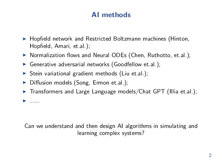
physics and generative AI, including normalization flows, generative adversary
networks, and transformers. Through algorithms and numerical examples, the
TIGC project builds on concrete and solid mathematical foundations of AI with
various applications in uncertainty quantification, sampling algorithms, and statistical
physics-related simulations.

Transcript

1. Transport Information Geometric Computations Wuchen Li University of South Carolina AFOSR PI meeting, August, 2025. Supported by AFOSR YIP 2023.
2. AI methods I Hopfield network and Restricted Boltzmann machines (Hinton, Hopfield, Amari, et.al.); I Normalization flows and Neural ODEs (Chen, Ruthotto, et.al.); I Generative adversarial networks (Goodfellow et.al.); I Stein variational gradient methods (Liu et.al.); I Di↵usion models (Song, Ermon et.al.); I Transformers and Large Language models/Chat GPT (Illia et.al.); I ...... Can we understand and then design AI algorithms in simulating and learning complex systems? 2
3. Geometry, Divergences, Sampling Taxonomy of principal distances and divergences Euclidean geometry Information geometries Euclidean distance d2 (p, q) = pP i (pi qi )2 (Pythagoras’ theorem circa 500 BC) Minkowski distance (Lk -norm) dk (p, q) = k pP i |pi qi |k (H. Minkowski 1864-1909) Manhattan distance d1 (p, q) = P i |pi qi | (city block-taxi cab) Mahalanobis metric (1936) d⌃ = p (p q)T ⌃ 1(p q) Quadratic distance dQ = p (p q)T Q(p q) Riemannian metric tensor R q gij dxi ds dxj ds ds (B. Riemann 1826-1866,) Physics entropy JK 1 k R p log pdµ (Boltzmann-Gibbs 1878) Information entropy H(p) = R p log pdµ (C. Shannon 1948) Fisher information (local entropy) I(✓) = E[ @ @✓ ln p(X|✓) 2 ] (R. A. Fisher 1890-1962) Kullback-Leibler divergence KL(p||q) = R p log p q dµ = E p [log P Q ] (relative entropy, 1951) R´ enyi divergence (1961) H↵ = 1 ↵(1 ↵) log R f↵dµ R ↵ (p|q) = 1 ↵(↵ 1) ln R p↵q 1 ↵dµ (additive entropy) Tsallis entropy (1998) (Non-additive entropy) T↵ (p) = 1 1 ↵ ( R p↵dµ 1) T↵ (p||q) = 1 1 ↵ (1 R p↵ q↵ 1 dµ) Bregman divergences (1967): BF (✓1 ||✓2 ) = F(✓1 ) F(✓2 ) (✓1 ✓2 )>rF(✓2 ) Bregman-Csisz´ ar divergence (1991) F↵ (x) = ⇢ x log x 1 ↵ = 0 x log x x + 1 ↵ = 1 1 ↵(1 ↵) ( x↵ + ↵x ↵ + 1) 0 < ↵ < 1 Csisz´ ar’ f-divergence Df (p||q) = R pf(q p )dµ (Ali& Silvey 1966, Csisz´ ar 1967) Amari ↵-divergence (1985) f↵ (x) = ⇢ x log x ↵ = 1 log x ↵ = 1 4 1 ↵ 2 (1 x 1+↵ 2 ) 1 < ↵ < 1 Quantum entropy S(⇢) = kTr(⇢ log ⇢) (Von Neumann 1927) Kolmogorov K(p||q) = R |q p|dµ (Kolmogorov-Smirnoff max |p q|) Hellinger H(p||q) = qR ( p p p q)2 = p 2(1 p fg Cherno↵ divergence (1952) C↵ (p||q) = ln R p↵q 1 ↵dµ C(p, q) = max ↵2(0,1) C↵ (p||q) 2 test 2(p||q) = R (q p)2 p dµ (K. Pearson, 1857-1936 ) Matsushita distance (1956) M↵ (p, q) = ↵ qR |q 1 ↵ p 1 ↵ |dµ Bhattacharya distance (1967) d(p, q) = log qR p p p qdµ Non-additive entropy cross-entropy conditional entropy mutual information (chain rules) Additive entropy Non-Euclidean geometries Statistical geometry Je↵rey divergence (Jensen-Shannon) H(p) = KL(p||u) Earth mover distance (EMD 1998) ⇥↵(1 ↵) ↵ = 1 ↵ = 0 Generalized Pythagoras’ theorem (Generalized projection) I-projection Quantum & matrix geometry Log Det divergence D(P||Q) =< P, Q 1 > log det PQ 1 dimP Von Neumann divergence D(P||Q) = Tr(P(log P log Q) P + Q) Itakura-Saito divergence IS(p|q) = P i (pi qi log pi qi 1) (Burg entropy) T Kullback-Leibler r⇤ Hamming distance (|{i : pi 6= qi }|) Neyman Dual div. (Legendre) DF ⇤ (rF(✓1 )||rF(✓2 )) = DF (✓2 ||✓1 ) Generalized f-means duality... Dual div.⇤-conjugate (f ⇤(y) = yf(1/y)) Df ⇤ (p||q) = Df (q||p) Burbea-Rao or Jensen (incl. Jensen-Shannon) JF (p; q) = f(p)+f(q) 2 f p+q 2 Integral probability metrics IPMs Wasserstein distances W↵,⇢(p, q) = (inf 2 (p,q) ⇢(p, q)↵ d (x, y)) 1 ↵ ⇢ = L1 L´ evy-Prokhorov distance LP ⇢ (p, q) = inf ✏>0 {p(A)  q(A✏) + ✏8A 2 B(X)} A✏ = {y 2 X, 9x 2 A : ⇢(x, y) < ✏} Finsler metric tensor gij = 1 2 @ 2 F 2(x,y) @yi@yj Sharma-Mittal entropies h↵, (p) = 1 1 ✓ R p↵ dµ 1 1 ↵ 1 ◆ = 1 ! ↵ Fisher-Rao distance: ds 2 = gij d✓id✓j = d✓ > I(✓)d✓ ⇢F R (p, q) = min R 1 0 p ˙ (t)I(✓) ˙ (t)dt Haussdorf set distance dH (X, Y ) = max{sup x ⇢(x, Y ), sup y ⇢(X, y)} Gromov-Haussdorf distance Sinkhorn divergence (h-regularized OT) (between compact metric spaces) dGH (X, Y ) = inf X :X!Z, Y :Y !Z {⇢Z H ( X (X), Y (Y ))} X , Y : isometric embeddings MMD Maximum Mean Discrepancy Stein discrepancies 2023 Frank Nielsen Optimal transport geometry Logarithmic divergence LG,↵(✓1 : ✓2) = 1 ↵ log 1 + ↵rG(✓2) > (✓1 ✓2) +G(✓2) G(✓1) ↵ ! 0, F = G A ne di↵erential geometry Riemannian geometry Hyperbolic/spherical geometry Bolyai (1802-1860) Lobachevsky (1792-1856) Aitchison distance Probability simplex Hilbert log-ratio metric Quantum f-divergences (D´ enes Petz) Fr¨ obenius & Hilbert-Schmidt norm J. Jensen F. Itakura B. De Finetti G. Monge L. Kantorovich M. Nagumo Pearson K. Nomizu L. LeCam Vajda M. Fr´ echet J.M. Souriau J.L. Koszul Symplectic geometry Cone geometry E. Vinberg Bhat. Conformal geometry Conformal divergence D⇢ (p : q) = ⇢(p)D(p : q) conformal Riemannian metric gphi = e g Dually flat space Constant sectional curvature Hessian manifolds H. Shima r Lev M. Bregman C. R. Rao B. Riemann Euclid Pythagoras Pal & Wong 2016 3
4. Information geometry Information matrix (a.k.a Fisher information matrix, Fisher–Rao metric) plays important roles in estimation, information science, statistics and machine learning: I Population Games via Replicator Dynamics (Shahshahani, Smith); I Machine learning: Natural gradient (Amari); Adam (Kingma 2014); Stochastic relaxation (Malago) and many more in the book Information geometry (Ay et.al.). I Statistics: Likelihood principle; Cramer-Rao bound, etc. I Optimization: Bregman divergences; Mirror descent, etc. 4
5. Optimal transport and mean field control In recent years, optimal transport (a.k.a Earth mover’s distance, Monge-Kantorovich problem, Wasserstein metric) has witnessed a lot of applications: I Mean field games (Larsy, Lions, Gangbo, et.al.); Population Games via Fokker-Planck Equations (Degond et. al. 2014, Li et.al. 2016); I Generalized Wasserstein gradient flows, Gamma calculuses, Ricci curvature lower bounds (Otto, Villani, Carrillo, Slepcev, Lott, Sturm, et.al.); I Machine learning: Wasserstein Training of Boltzmann Machines (Cuturi et.al. 2015); Learning from Wasserstein Loss (Frogner et.al. 2015); Wasserstein GAN (Bottou et.al. 2017); I Reviews: A mean field games laboratory for generative modeling (Zhang, Katsoulakis, 2023); Variational and Information Flows in Machine Learning and Optimal Transport (2025)... 5
6. Information matrix and Pull back 6
7. Statistical information matrix Definition (Statistical Information Matrix) Consider the density manifold (P(X), g) with a metric tensor g, and a smoothly parametrized statistical model p✓ with parameter ✓ 2 ⇥ ⇢ Rd. Then the pull-back G of g onto the parameter space ⇥ is given by G(✓) = D r✓p✓, g(p✓)r✓p✓ E . Denote G(✓) = (G(✓)ij)1i,jd , then G(✓)ij = Z X @ @✓i p(x; ✓) ⇣ g(p✓) @ @✓j p ⌘ (x; ✓)dx. Here we name g the statistical metric, and call G the statistical information matrix. 7
8. Score Function Definition (Score Function) Denote i : X ⇥ ⇥ ! R, i = 1, ..., n satisfying i(x; ✓) =  g(p) ✓ @ @✓i p(x; ✓) ◆ . They are the score functions associated with the statistical information matrix G and are equivalent classes in C(X)/R. The representatives in the equivalent classes are determined by the following normalization condition: E p✓ i = 0, i = 1, ..., n. Then the statistical metric tensor satisfies G(✓)ij = Z X i(x; ✓) ⇣ g(p✓) 1 j ⌘ (x; ✓)dx. 8
9. Example: Fisher-Rao metric I The Fisher-Rao metric comes from Information Geometry. I The inverse of the Fisher-Rao metric tensor is defined by GF (⇢) 1 = ⇢ ✓ Z ⇢dx ◆ , 2 T⇤ ⇢ P(⌦). I For 1, 2 2 T⇢ P(⌦), the Fisher-Rao metric on the tangent space follows gF ⇢ ( 1, 2) = Z 1 2⇢dx ✓Z 1⇢dx ◆ ✓Z 2⇢dx ◆ , where i is the solution to i = ⇢ i R i⇢dx , i = 1, 2. 9
10. Example: Wasserstein metric I The Wasserstein metric comes from Optimal Transport1. I The inverse of the Wasserstein metric tensor is defined by GW (⇢) 1 = r · (⇢r ), 2 T⇤ ⇢ P(⌦). I The Wasserstein metric on the tangent space is given by gW ⇢ ( 1, 2) = Z ⇢hr 1, r 2 idx, 1, 2 2 T⇢ P(⌦), where i is the solution to i = r · (⇢r i), i = 1, 2. 1C´ edric Villani. Topics in optimal transportation. American Mathematical Soc., 2003. 10
11. Transport information geometry Main Question: Analyzing and constructing AI methods for simulating complex systems. Related studies I Wasserstein covariance (Petersen, Muller ...) I Wasserstein natural gradient (Li, Montufar, Chen, Lin, Abel, Liu ...) I Wasserstein divergences (Wang, Pal, Guo, Li, Ay ...) I Wasserstein statistics (Amari, Li, Matsuda, Zhao, Rubio ...) I Wasserstein fluctuation and non-equilibrium thermodynamics (Ito, Kobayashi, Li, Liu, Gao ...) I Wasserstein di↵usions and Dean-Kawasaki dynamics (Renesse, Sturm, Li ...) I Stochastic Dynamical density functional theory (SDDFT). 11
12. Current studies in 2024-2025 I Score based neural ODEs in simulating Fokker-Planck equations; I Natural Primal-dual hybrid gradient in solving PDEs; I Accelerated sampling schemes in continuous and discrete domains; I Sparse and Preconditoned regularized Wasserstein proximal operators for sampling target distributions; 12
13. Score-based normalizing flow with application in mean field control Mo Zhou, Stanley Osher, Wuchen Li arXiv:2506.05723v2, Aug 2025
14. Introduction I The score function, defined as the gradient of the logarithm of the density function rx log ⇢(t, x), plays a central role in modern AI and second order Mean field control problems. I We develop the score-based normalizing flow as a computational framework for approximating the score function. One aims to minimize the cost inf v Z T 0 Z Rd [L(t, x, v(t, x)) + F(t, x, ⇢(t, x))] | {z } running cost ⇢(t, x) dx dt + Z Rd G(x, ⇢(T, x)) | {z } terminal cost ⇢(T, x) dx subject to the Fokker–Planck equation @t⇢(t, x) + rx · (⇢(t, x)v(t, x)) = x ⇢(t, x) , ⇢(0, x) = ⇢0(x). 2
15. Formulations We compute the score function st = rx log ⇢(t, xt) along the trajectory @t xt = f (t, xt) through @t st = d dt rx log ⇢(t, xt) = rx f (t, xt) >st rx (rx · f (t, xt)). Then, we reformulate the mean field control problem as inf f Z T 0 Z Rd [L(t, x, f (t, x) + rx log ⇢(t, x)) + F(t, x, ⇢(t, x))] ⇢(t, x) dx dt + Z Rd G(x, ⇢(T, x))⇢(T, x) dx subject to the continuity equation @t⇢(t, x) + rx · (⇢(t, x)f (t, x)) = 0 , ⇢(0, x) = ⇢0(x). 3
16. Example: Regularized Wasserstein proximal operator Consider inf v Z 1 0 Z Rd 1 2 |v(t, x)|2 ⇢(t, x) dx dt + Z Rd G(x)⇢(1, x) dx , s.t. @t⇢(t, x) + rx · (⇢(t, x)v(t, x)) = x ⇢(t, x). Figure: Terminal histogram and density evolution of a Regularized Wasserstein Proximal Operator (RWPO) example with double well potential in 1 dimension. 4
17. Example: Flow matching for stochastic Lorenz 63 system Consider 8 > > < > > : dxt = (yt xt) dt + p 2" dW x t , dyt = (xt(⇢ zt) yt) dt + p 2" dW y t , dzt = (xt yt zt) dt + p 2" dW z t . Figure: Projection of 3D stochastic Lorenz system to x-y plane. 5
18. Future work I Analyze the accuracy of score based neural ODEs; I Simulate Fokker-Planck equations with variable di↵usion matrices. 6
19. Adversarial learning for partial differential equations using natural gradients Shu Liu, Stanley Osher, Wuchen Li August, 2025 ArXiv links: https://arxiv.org/abs/2411.06278.
20. Motivation I Deep learning for high-dim partial differential equations (PDEs): I Key ingredients for deep learning PDE solver: – Loss function: I Residual of PDE, High-order derivative pathology; I Energy functional, Restrictive to variational problems; I Weak form of PDE,Versatile, Get rid of high-order differentiation, min-max problem. – Optimizer: I First-order method: SGD, Adam, etc. Strong fluctuation, spikes; I Quasi-Newton method: L-BFGS, Unstable w.r.t. random batch; I Natural Gradient, Stable, Higher accuracy. I Goal: Develop a versatile approach that addresses ill-conditioned loss while mitigating training instability. 2
21. Our treatment Weak form + Natural Gradients Adversarial learning Preconditioned gradients Natural Primal-Dual Gradient (NPDG) method I We derive the NPDG algorithm for the Poisson equation: u = f , on ⌦, u = g, on @⌦. (1) I Introduce primal neural network u ✓ ; Multiply (1) with discriminator networks ', ⇠ ; Integration by parts yields: inf ✓ sup ⌘,⇠ E (u ✓, '⌘, ⇠) := Z ⌦ ru ✓ · r'⌘ f '⌘ dx + Z @⌦ (u ✓ g) ⇠ d 1 2 ✓Z ⌦ kr'⌘k2dx + Z @⌦ 2 ⇠ d ◆ . I This inf-sup approach originates from the weak formulation of PDEs with quadratic regularization. 3
22. NPDG algorithm Alternative Natural gradients (NGs) with extrapolation (n 1):  ⌘n+1 ⇠n+1 =  ⌘n ⇠n + ⌧' " M(⌘n )† @ @⌘ E (u ✓n , '⌘n , ⇠n ) M(⇠n )† @ @⇠ E (u ✓n , '⌘n , ⇠n ) # , NG ascent  e 'n+1 e n+1 =  '⌘n+1 ⇠n+1 + ! ✓ '⌘n+1 ⇠n+1  '⌘n ⇠n ◆ , Extrapolation ✓n+1 = ✓n ⌧u Mp(✓n )† @ @✓ E (u ✓n , e 'n+1, e n+1). NG descent (⌧', ⌧u > 0 are optimization stepsize, ! > 0 is the extrapolation coefficient.) (M(✓))ij = Z ⌦ @ @✓i ru ✓(x) · @ @✓j ru ✓(x)dx + Z @⌦ @u ✓(x) @✓i @u ✓(x) @✓j d . (M(⌘))ij = Z ⌦ @ @⌘i r'⌘(x) · @ @⌘j r'⌘(x)dx; (M(⇠))ij = Z @⌦ @ ⇠(x) @⌘i @ ⌘(x) @⌘j d . I The decomposition of the Laplacian motivates the choice of preconditioning matrices: h u, 'i = hru, r'i, u 2 H2(⌦), ' 2 H1 0 (⌦). I The pseudoinverse is computed using Krylov subspace iterations, ensuring a scalable approach. 4
23. Operator-Informed Preconditioning: Fast & smoother convergence I Comparison with commonly used deep learning PDE-solvers. PINN(Adam): Residual minimized by Adam; DeepRitz: Energy functional minimized by Adam; WAN: Weak form optimized by Adam; NPDG: Our method. 5
24. Capacity for achieving higher accuracy I GPU time(seconds) required to reach relative L2 accuracy . I Fix NN architecture and sample size for all tested methods. Note: “–” the accuracy is never achieved; “N.A.” method is not applicable. All equations are posed with Dirichlet boundary conditions. 6
25. Adversarial Learning Scheme: Versatility Our algorithm has a broad application: semilinear equations, reaction-diffusion equations, Monge-Ampère equations (Optimal Transport), etc. |det(D2u(x))| = ⇢0(x) ⇢1(ru(x)) , ⇢0 dx a.e., u is convex on Rd . ru : Rd ! Rd is the optimal mapping T : Rd ! Rd, pushing forward standard Gaussian ⇢0 to mixed Gaussian ⇢1 while minimizing R Rd kT(x) xk2⇢0(x) dx. Figure: Plots of the pushforwarded density T ✓]⇢0 . Left: NPDG method; Right: Primal-Dual algorithm using Adam. Red lines indicate the computed OT map. 7
26. Outlook NPDG algorithm: Efficient scientific machine learning (SciML) paradigm. Applicable to large-scale saddle point/constrained optimization problems: I Enhancing the training of Generative Adversarial Networks (GANs). [Goodfellow, et al. 2014], [Arjovsky, et al. 2017]... I Optimal Transport (Monge) problem with general cost. [Fan, Liu, et al. 2021], [Asadulaev, Korotin, et al. 2022]... I High-dimensional Mean-Field Control problems. [Ruthotto, et al. 2019], [Lin, Wu Fung, et al. 2020]... Primary objective: Update the parameters of the generator network G ✓ and the discriminator network D ⌘ using natural gradients. 8
27. Accelerated MCMC on Discrete States Wuchen Li (USC) joint work with Bohan Zhou (UCSB), Shu Liu (UCLA), Xinzhe Zuo (UCLA) arXiv:2505.12599 August 11, 2025
28. Introduction Consider sampling from a discrete space (data has some intrinsic structure like graph), Figure: MCMC on the discrete space of phylogenetic trees. Figure credit to Matsen group. I How can we design a Nesterov accelerated sampling algorithm on discrete state spaces? I What is the accelerated dynamics with discrete score functions? 2
29. Formulations Damped Hamitonian Flow 3
30. Methods Given a graph weight !ij = ⇡iQij, for a pair of variables (pi, i), consider 8 > > > > < > > > > : dpi dt + X j6=i !ij✓ij(p)( j i) = 0, d i dt + (t) i + 1 2 X j6=i !ij @✓ij(p) @pi ( i j)2 + @U(p) @pi = 0. I Activation function ✓ij(p); I Potential function U(p); I Damping parameter (t) > 0. 4
31. Example I: 2 method ✓ij = 1, U(p) = 1 2 Pn i=1 (pi ⇡i)2 ⇡i , and = 2 p |↵⇤ |, where ↵⇤ is the largest negative eigenvalue to Q. Figure: Sampling on a 3-node graph. The target distribution is concentrated on node 1. Figure: The decay of log10 kp(t) ⇡k2 . 5
32. Example II: the relative Fisher method ✓ij(p) = pj ⇡j pi ⇡i log ⇡ipj ⇡j pi U(p) = 1 4 n X i=1 X j6=i !ij(log pi ⇡i log pj ⇡j )( pi ⇡i pj ⇡j ) Figure: Sampling on a 25 ⇥ 25 lattice graph. 6
33. Example II (cont.): Gaussian Mixture on lattices 7
34. Accelerated Stein Variational Gradient Flow Viktor Stein and Wuchen Li Viktor Stein, Technical University of Berlin https://arxiv.org/abs/2503.23462 https://github.com/ ViktorAJStein/Accelerated_ Stein_Variational_Gradient_Flows
35. Sampling using Stein Variational Gradient Descent (SVGD) Liu & Wang, NeurIPS’16 Task: sample density ⇡ / e V with potential V : Rd ! R. Applications: Bayesian inference, uncertainty quantification. Symmetric, positive definite, di↵erentiable “kernel” K : Rd ⇥ Rd ! R. SVGD update in the n-th iteration with step size ⌧ > 0: x n+1 i x n i ⌧ N ✓ N X j=1 K(x n i , x n j )rV (x n j ) | {z } attraction N X j=1 r2K(x n i , x n j ) | {z } repulsion ◆ . ; SVGD is gradient descent of KL(· | ⇡) with respect to a ”Stein geometry” (induced by K) when replacing ⇢ by a sample average. 2
36. Gradient flows in the density manifold forms an infinite-dimensional smooth Fr´ echet manifold. Metric tensor field on e P(⌦) is a smooth map G: e P(⌦) 3 ⇢ 7! G⇢. Stein metric defined via: (G (K) ⇢ ) 1( ) := ✓ x 7! rx · ✓ ⇢(x) Z ⌦ K(x, y)⇢(y)r (y) dy ◆◆ . Definition (Metric gradient flow on e P(⌦)) A smooth curve ⇢: [0, 1) ! e P(⌦), t 7! ⇢t is a (e P(⌦), G)-gradient flow of E starting at ⇢(0) if @t⇢t = G 1 ⇢t [ E(⇢t)], 8t > 0. Intuition: inverse metric tensor deforms linear derivative E. 3
37. Accelerated Stein variational gradient flow on densities The Hamiltonian on e P(⌦) is H : T e P(⌦) ! R [{1}, (⇢, ) 7! 1 2 Z ⌦ (x)G 1 ⇢ [ ](x) dx + E(⇢). As before: ⇢ = position, = momentum. We have 2H(⇢, ) = G 1 ⇢ [ ], so accelerated gradient flow in e P(⌦) is 8 < : @t⇢t = G 1 ⇢t [ t] @t t + ↵t t + 1 2 ⇢Z ⌦ t(x)G 1 • [ t](x) dx (⇢t) + E(⇢t) = 0. ; accelerated Stein variational gradient flow is ( @t⇢t + r · ⇢t R ⌦ K(·, y)⇢t(y)r t(y) dy = 0, @t t + ↵t t + R ⌦ K(y, ·)hr t(y), r t(·)i⇢t(y) dy + E(⇢t) = 0. 4
38. Score-free particle discretization - integrating by parts Use particle momentum Y : (0, 1) ! Rd , t 7! ˙ Xt, ˙ Xt = Yt = Z ⌦ K(Xt, y)r t(y)⇢t(y) dy. Key idea of SVGD: use integration by parts to shift derivative from density ⇢ to the kernel K. ; can be applied in the accelerated scheme: Lemma (Accelerated Stein variational gradient flows with particles’ momenta) The associated deterministic interacting particle system is 8 > > > > > > > > < > > > > > > > > : ˙ Xt = Yt, ˙ Yt = ↵tYt + Z ⌦ (K(Xt, y)rV (y) r2K(Xt, y)) ⇢t(y) dy + Z ⌦2 hr t(z), r t(y)i ·  K(y, z)(r2K)(Xt, y) +K(Xt, z)(r1K)(Xt, y) K(Xt, y)(r2K)(z, y) ⇢t(y) dy ⇢t(z) dz. ; replace expectation w.r.t. ⇢t by sample averages. 5
39. Numerical examples - Gaussian kernel Particle trajectories. ASVGD, SVGD, with Gaussian kernel, MALA, and ULD (from left to right) for V (x, y) = 1 4 (x4 + y4) (convex, non-Lipschitz) (top), the double bananas target (middle) and an anisotropic Gaussian target (bottom). Double bananas target: constant high damping = 0.985. Other targets: speed restart and gradient restart. 6
40. Numerical examples - Bayesian Neural Network RMSE Log-likelihood execution time (s) Dataset ASVGD SVGD ASVGD SVGD ASVGD SVGD Concrete 5.536±0.060 7.349±0.067 3.135±0.016 3.439±0.010 14.867±0.040 14.001±0.044 Energy 0.899±0.057 1.950±0.028 1.268±0.068 2.088±0.016 14.870±0.051 13.942±0.035 Housing 2.346±0.077 2.386±0.048 2.305±0.020 2.343±0.014 18.278±0.045 17.214±0.077 Kin8mn 0.118±0.001 0.165±0.001 0.71±0.011 0.384±0.004 14.859±0.029 14.001±0.033 Naval 0.005±0.0 0.007±0.0 3.801±0.01 3.504±0.003 20.912±0.57 19.704±0.05 power 3.951±0.005 4.035±0.008 2.799±0.001 2.825±0.002 12.142±0.053 11.435±0.054 protein 4.777±0.007 4.987±0.009 2.983±0.001 3.026±0.002 15.616±0.04 14.752±0.047 wine 0.185±0.013 0.191±0.017 0.201±0.039 0.146±0.046 18.293±0.097 17.244±0.077 Table: Test root mean square error (RMSE, lower is better) and log-likelihood (LL, higher is better) after 2000 iterations, without restarts and constant damping = 0.95, M = 10 particles 7
41. Discussions I Find best kernel parameters A and 2 . I Find best choice of damping function ↵t = ↵ t . I Conformal symplectic discretization instead of explicit Euler (retains structure of continuous dynamics). I Investigate bias of the algorithm. I Incorporate annealing strategy. I Finite particle convergence guarantees. 8
42. Splitting Regularized Wasserstein Proximal Algorithms for Nonsmooth Sampling Problems Fuqun HAN (UCLA), Stanley Osher (UCLA) and Wuchen Li (USC) arXiv:2502.16773, 2025
43. Introduction I Objective: Generate a sequence of samples {xk j }N j=1 that approximates a target distribution, known up to a constant through its density function: ⇢⇤(x) = 1 Z exp( V (x)), where Z is the normalization constant. I We are particularly interested in the case where V = f + g, with g representing a regularization term. I Examples of applications: Generative modeling and Bayesian inference. I We propose explicit and semi-implicit discretization of the ODE: dxt = rV (xt) dt 1r log ⇢t(xt) dt, where r log ⇢t(xt) is the score function. 2
44. Regularized Wasserstein Proximal Operator I We define the regularized Wasserstein proximal operator (RWPO) as WProxh, V (⇢k) := arg min q2P2(Rd) inf v ⇢Z Rd V (x)q(x) dx + Z h 0 Z Rd 1 2 kv(t, x)k2 2 ⇢(t, x) dx dt , subject to @⇢ @t + r · (⇢v) = 1 ⇢, ⇢(0, x) = ⇢k(x), ⇢(h, x) = q(x). I The RWPO is a first-order approximation to the evolution of Fokker Plank equation. I Through the Hopf-Cole transform, it has a closed-form solution: WProxh, V (⇢k)(x) = Z Rd exp  2 ✓ V (y) + kx yk2 2 2h ◆ R Rd exp  2 ✓ V (z) + kz yk2 2 2h ◆ dz ⇢k(y) dy =: Kh V ⇢k(x). 3
45. Splitting of Composite Potentials with L1 Prior I When V (x) = f(x) + g(x), we split the iterative scheme into smooth and nonsmooth parts to have ( xk+ 1 2 = xk hrf(xk), xk+1 = proxh g (xk+ 1 2 ) h 1r log Kh g ⇢ k+ 1 2 (xk+ 1 2 ), where Kh g ⇢k+ 1 2 ⇡ ⇢k+1 . I The scheme is semi-implicit since we approximate r log ⇢k+1 , and it is closed due to the kernel formula. I When g(x) = kxk1 , the proximal operator is the soft-thresholding function: S h(x) := proxh kxk1 (x) = sign(x) max{|x| h, 0} and the score function can be approximated via Laplace approximation: r log Kh g ⇢k(x) ⇡ 2 0 B @ x S h(x) h + PN j=1 (x xk+ 1 2 j ) exp(U(x, xk+ 1 2 j )) h PN j=1 exp(U(x, xk+ 1 2 j )) 1 C A , with some interaction kernel U. 4
46. Example I: Gaussian Mixture 0 50 100 150 200 250 300 350 400 iteration 0.3 0.4 0.5 0.6 0.7 0.8 0.9 D KL ( 1 || 1 * ) BRWP PRGO MYULA 0 50 100 150 200 250 300 350 400 iteration 0 0.1 0.2 0.3 0.4 0.5 0.6 0.7 0.8 0.9 1 D KL ( d || d * ) BRWP PRGO MYULA Figure: Example 1: Results in d = 50, step size h = 0.02, and 100 particles. From left to right: KL divergence decay and density approximations by BRWP-splitting and MYULA. 5
47. Example II: TV Denoising We consider g(x) = kDxk1 as the total variation term. Figure: Example 2: From left to right: exact image, noisy image, and denoised means after 100 iterations by BRWP-splitting and MYULA. 6
48. Ongoing work: Sparse Transformer 7
49. Sampling via preconditioned regularized Wasserstein proximals Hong Ye Tan, Stanley Osher, Wuchen Li On-going work. arXiv:2509.01685
50. Preconditioned BRWP Algorithm Sampling / exp( V (x)/ ) for collection of particles X = ⇥ x1 ... xN ⇤ 2 Rd⇥N : X(k+1) = X(k) ⌘ 2 M rV (X(k)) | {z } dynamics + ⌘ 2T ⇣ X(k) X(k)softmax(W(k))> ⌘ | {z } di↵usion where interaction matrix W(k) ij = kxi xj k2 M 4 T log Z Rd e 1 2 (V (z)+ kz xj k2 M 2T ) dz. 2
51. Transformer related sampler Transformer structure (up to scaling): Attn(Q; K, V ) = softmax QK> V. Self attention: X 7! Attn(Q(X); K(X), V (X)) X(k+1) = X(k) ⌘ 2 MrV (X(k)) + ⌘ 2T ⇣ X(k) X(k)softmax(W(k))> ⌘ W(k) ij = kxi xj k2 M 4 T log Z Rd e 1 2 (V (z)+ kz xj k2 M 2T ) dz | {z } =:Rj . Di↵usion rewritten as masked-attention structure: (Red) = softmax(QK> + 1R>), QK> = 1 4 T X>M 1X, R = (Rj), V = X. (1) 3
52. Preconditioning the Regularized Wasserstein Proximal Adding Laplacian regularization to the Benamou–Brenier formulation: 8 > < > : @t⇢(t, x) + rx · (⇢(t, x)rx (t, x)) = x⇢(t, x), @t (t, x) + 1 2 krx (t, x)k2 = x (t, x), ⇢(0, x) = ⇢0(x), (T, x) = V (x). yields a kernel representation WProxT,V ⇢(x) = Z Rd K(x, y)⇢(y) dy, K(x, y) = exp( 1 2 (V (x) + kx yk2 2T )) R Rd exp( 1 2 (V (z) + kz yk2 2T )) dz . K is convolution with a heat kernel. 4
53. Methods To use a di↵erent kernel, consider M 2 Rd⇥d that is symmetric and positive definite, KM (x, y) = exp( 1 2 (V (x) + kx yk2 M 2T )) R Rd exp( 1 2 (V (z) + kz yk2 M 2T )) dz . Anisotropic heat kernel KM is Green’s function for anisotropic heat eq. @tu = r · (Mru) 5
54. Derivation By using Cole–Hopf transform on coupled anisotropic heat equations 8 > < > : @t ˆ ⌘(t, x) = r · (Mrˆ ⌘(t, x)) @t⌘(t, x) = r · (Mr⌘(t, x)), ⌘(0, x)ˆ ⌘(0, x) = ⇢0(x), ⌘(T, x) = e V (x)/2 + 8 > < > : @t⇢(t, x) + r · (⇢(t, x)r (t, M 1x)) = r · (Mr⇢)(t, x) @t (t, M 1x) + 1 2 kr (t, M 1x)k2 M = Tr(M 1(r2 )(t, M 1x)) ⇢(0, x) = ⇢0(x), (T, M 1x) = V (x) 6
55. Accelerated Di↵usion MALA MLA BRWP PBRWP Figure: Evolution of the various methods for the stretched annulus at iterations 10, 50, and 200. 7
56. High-dimensional deconvolution ULA MYULA MLA PBRWP Figure: Standard deviations for TV-regularized deconvolution at 20, 200, 2000 iterations. 8
57. Discussions I Study information matrix for constructing neural network architectures in scientific machine learning problems; I Design generalized transformers for sampling algorithms; I Construct Digital twins from transport information geometry. 13