Preconditioned Sampling and Sparse Transformer Architectures from Regularized Wasserstein Proximal Operators

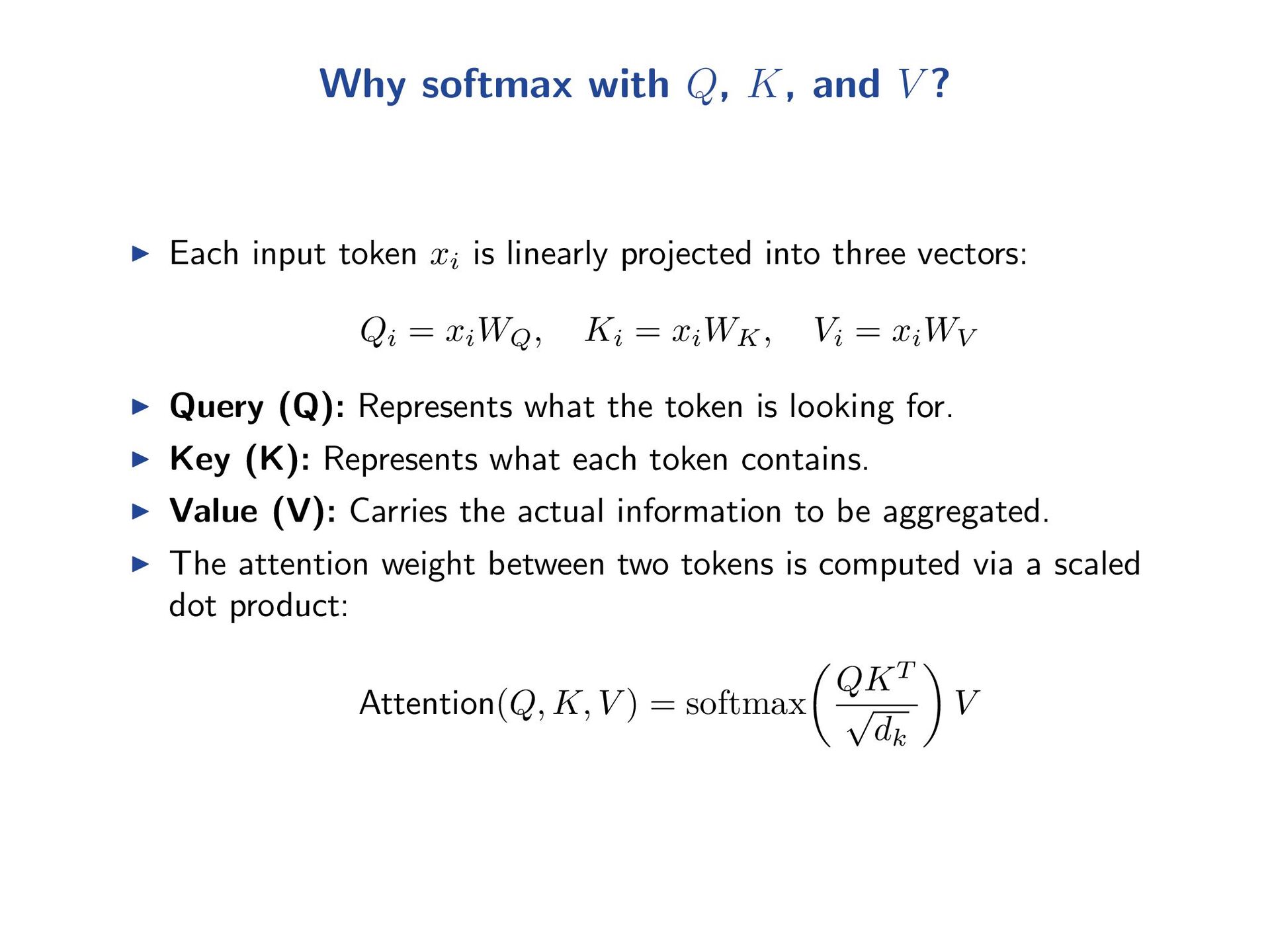
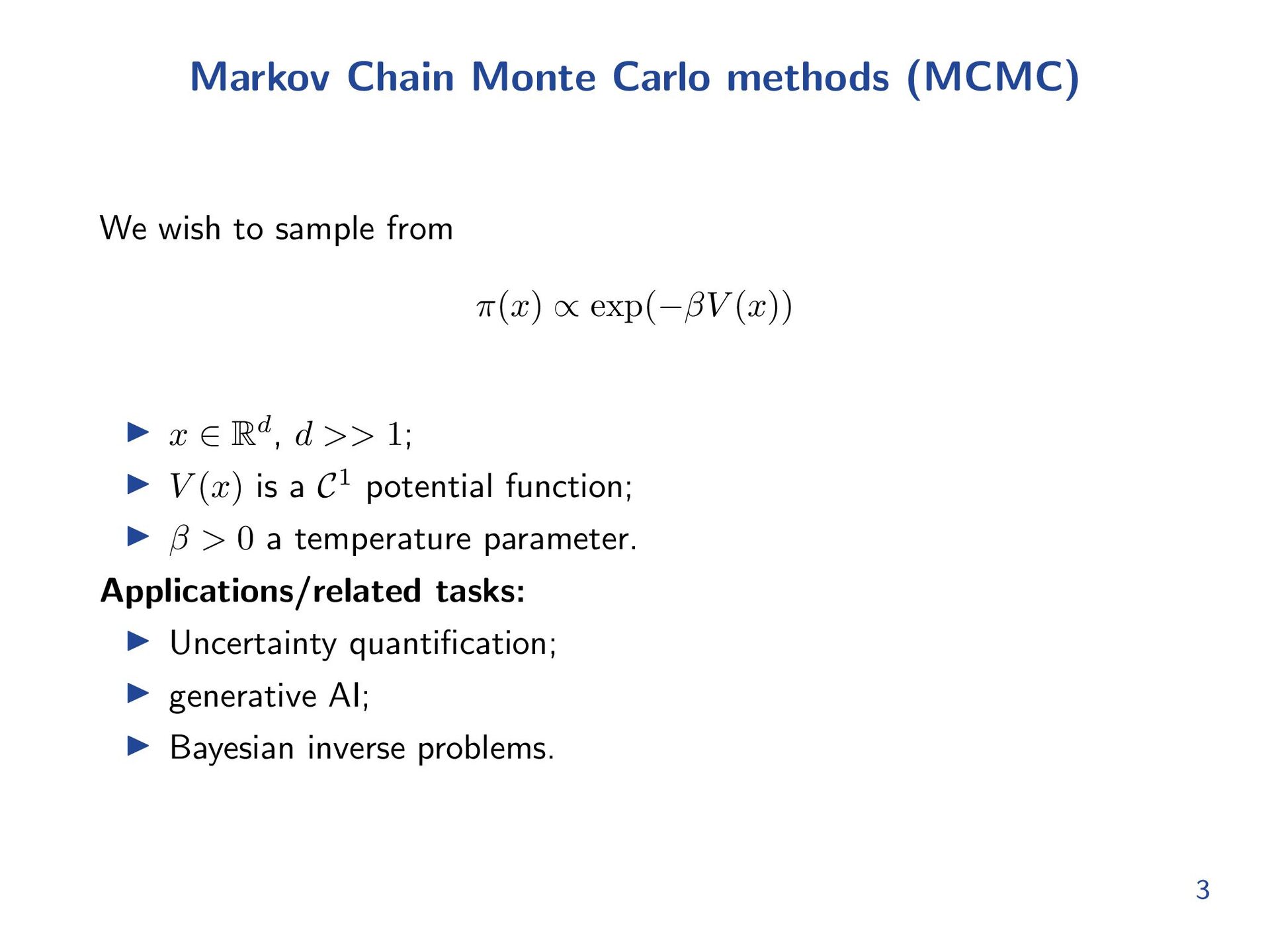
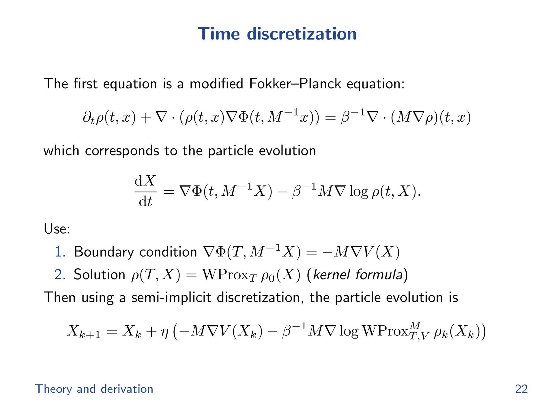
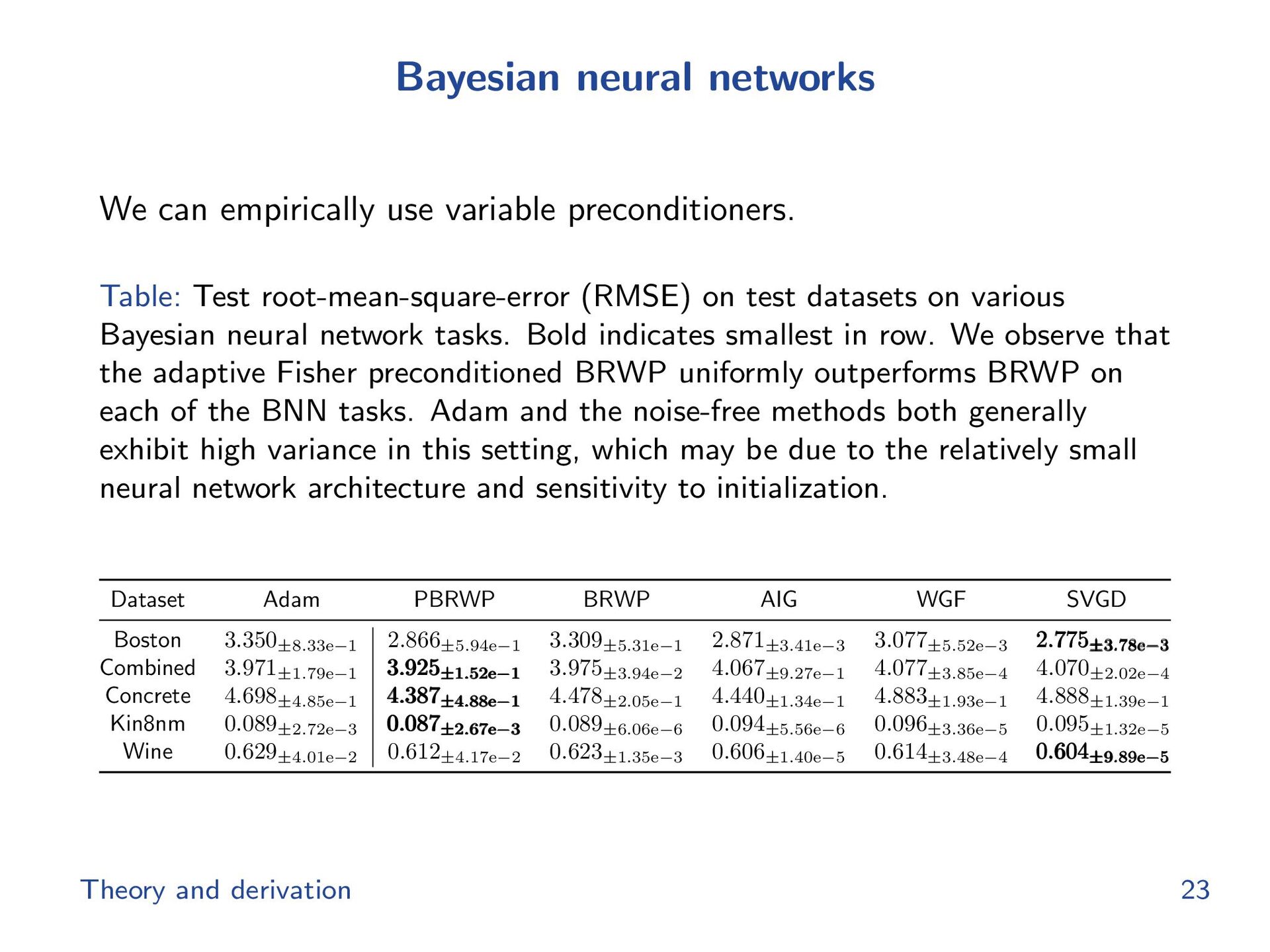
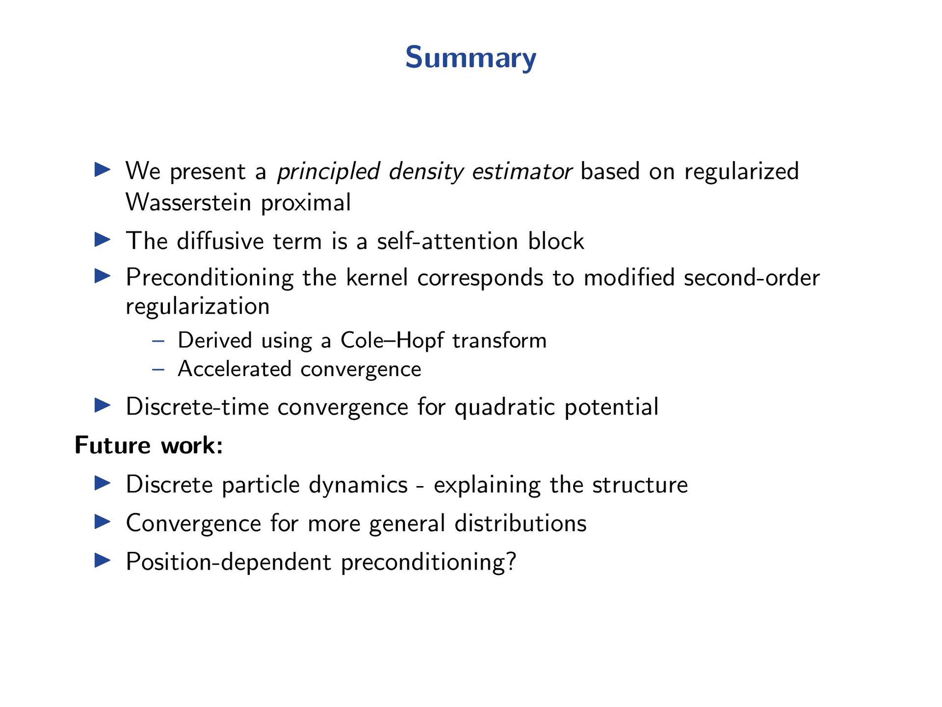
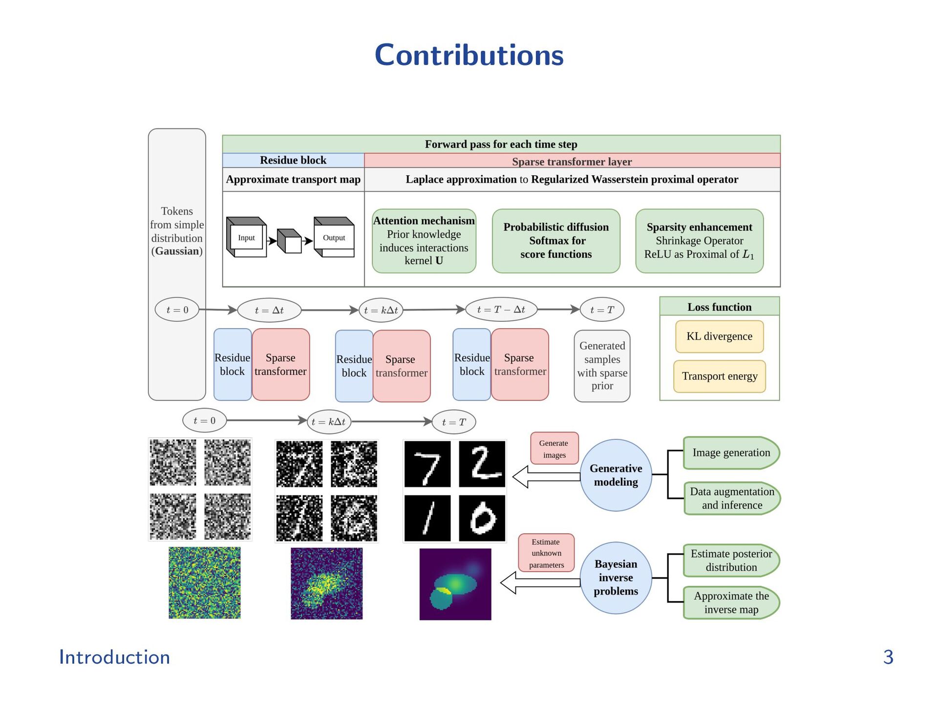
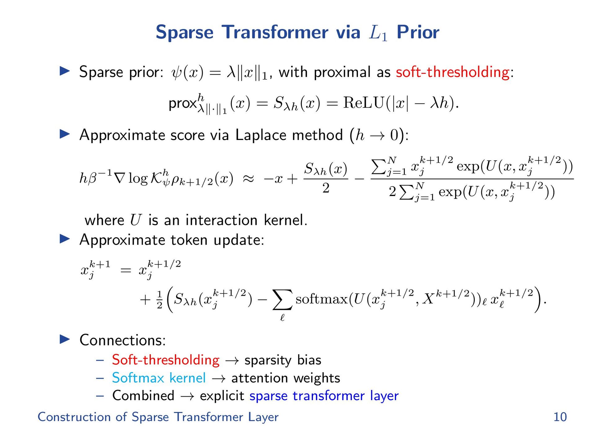
We present a unified framework connecting sampling algorithms, optimal transport, and transformer architectures. The approach introduces a preconditioned, noise-free sampling method based on the regularized Wasserstein proximal operator, derived via a Cole–Hopf transformation on anisotropic heat equations. Extending this connection, we design a sparse transformer architecture that embeds an L₁ prior to enhance convexity and promote sparsity of the learning problem. Theoretical results show non-asymptotic convergence with explicit bias characterization, and experiments demonstrate improved efficiency and accuracy across Bayesian neural networks, Bayesian inverse problems, and generative modeling of image distributions.

Transcript

1. Preconditioned Sampling and Sparse Transformer Architectures from Regularized Wasserstein Proximal Operators Wuchen Li University of South Carolina Level set seminar, Oct, 2025. These are mainly based on joint works with Fuqun Han, Hong Ye Tan, and Stanley Osher.
2. AI methods I Hopfield network and Restricted Boltzmann machines (Hinton, Hopfield, Amari, et.al.); I Normalization flows and Neural ODEs (Chen, Ruthotto, et.al.); I Generative adversarial networks (Goodfellow et.al.); I Stein variational gradient methods (Liu et.al.); I Di↵usion models (Song, Ermon et.al.); I Transformers and Large Language models/Chat GPT (Illia et.al.); I ...... Can we understand and then design AI algorithms in simulating and learning complex systems? Score functions.
3. Transformers I Key idea: sequence modeling via self-attention (no recurrence, no convolution). I Introduced by Vaswani et al. (2017): Attention Is All You Need, >= 199k citations since 2017. I Highly parallelizable; scales to billions of parameters. I Applications: language (GPT, BERT). Input Tokens Encoder Stack Decoder Stack Output Tokens
4. Self-Attention Mechanism Scaled Dot-Product Attention Attention(Q, K, V ) = softmax ✓ QK> p dk ◆ V I Q, K, V from linear projections of token embeddings. I Multi-head attention learns relationships in parallel subspaces. I Positional encodings inject order information.
5. Why softmax with Q, K, and V ? I Each input token xi is linearly projected into three vectors: Qi = xiWQ, Ki = xiWK, Vi = xiWV I Query (Q): Represents what the token is looking for. I Key (K): Represents what each token contains. I Value (V): Carries the actual information to be aggregated. I The attention weight between two tokens is computed via a scaled dot product: Attention(Q, K, V ) = softmax ✓ QKT p dk ◆ V
6. Divergences, Sampling, and Machine learning Taxonomy of principal distances and divergences Euclidean geometry Information geometries Euclidean distance d2 (p, q) = i (pi → qi )2 (Pythagoras’ theorem circa 500 BC) Minkowski distance (Lk -norm) dk (p, q) = k i |pi → qi |k (H. Minkowski 1864-1909) Manhattan distance d1 (p, q) = i |pi → qi | (city block-taxi cab) Mahalanobis metric (1936) d! = (p → q)T !→1(p → q) Quadratic distance dQ = (p → q)T Q(p → q) Riemannian metric tensor gij dxi ds dxj ds ds (B. Riemann 1826-1866,) Physics entropy JK →1 →k p log pdµ (Boltzmann-Gibbs 1878) Information entropy H(p) = → p log pdµ (C. Shannon 1948) Fisher information (local entropy) I(ω) = E[ ω ωε ln p(X|ω) 2 ] (R. A. Fisher 1890-1962) Kullback-Leibler divergence KL(p||q) = p log p q dµ = E p [log P Q ] (relative entropy, 1951) R´ enyi divergence (1961) Hϑ = 1 ϑ(1→ϑ) log fϑdµ R ϑ (p|q) = 1 ϑ(ϑ→1) ln pϑq 1→ϑdµ (additive entropy) Tsallis entropy (1998) (Non-additive entropy) Tϑ (p) = 1 1→ϑ ( pϑdµ → 1) Tϑ (p||q) = 1 1→ϑ (1 → pω qω→1 dµ) Bregman divergences (1967): BF (ω1 ||ω2 ) = F(ω1 ) → F(ω2 ) → (ω1 → ω2 )↑↑F(ω2 ) Bregman-Csisz´ ar divergence (1991) Fω (x) = x → log x → 1 ω = 0 x log x → x + 1 ω = 1 1 ω(1→ω) (→xω + ωx → ω + 1) 0 < ω < 1 Csisz´ ar’ f-divergence Df (p||q) = pf(q p )dµ (Ali& Silvey 1966, Csisz´ ar 1967) Amari ε-divergence (1985) fω (x) = x log x ω = 1 → log x ω = →1 4 1→ω 2 (1 → x 1+ω 2 ) →1 < ω < 1 Quantum entropy S(ϑ) = →kTr(ϑ log ϑ) (Von Neumann 1927) Kolmogorov K(p||q) = |q → p|dµ (Kolmogorov-Smirnoff max |p → q|) Hellinger H(p||q) = ( ↓ p → ↓ q)2 = 2(1 → ↓ fg Cherno! divergence (1952) Cϑ (p||q) = → ln pϑq 1→ϑdµ C(p, q) = max ϑ↓(0,1) Cϑ (p||q) ϖ 2 test ϖ 2(p||q) = (q→p)2 p dµ (K. Pearson, 1857-1936 ) Matsushita distance (1956) Mϑ (p, q) = ω |q 1 ω → p 1 ω |dµ Bhattacharya distance (1967) d(p, q) = → log ↓ p ↓ qdµ Non-additive entropy cross-entropy conditional entropy mutual information (chain rules) Additive entropy Non-Euclidean geometries Statistical geometry Je!rey divergence (Jensen-Shannon) H(p) = KL(p||u) Earth mover distance (EMD 1998) ↑ω(1 → ω) ω = →1 ω = 0 Generalized Pythagoras’ theorem (Generalized projection) I-projection Quantum & matrix geometry Log Det divergence D(P||Q) =< P, Q →1 > → log det PQ →1 → dimP Von Neumann divergence D(P||Q) = Tr(P(log P → log Q) → P + Q) Itakura-Saito divergence IS(p|q) = i (pi qi → log pi qi → 1) (Burg entropy) Kullback-Leibler →→ Hamming distance (|{i : pi ↑= qi }|) Neyman Dual div. (Legendre) DF ↔ (↑F(ω1 )||↑F(ω2 )) = DF (ω2 ||ω1 ) Generalized f-means duality... Dual div.↓-conjugate (f ↓(y) = yf(1/y)) Df ↓ (p||q) = Df (q||p) Burbea-Rao or Jensen (incl. Jensen-Shannon) JF (p; q) = f(p)+f(q) 2 → f p+q 2 Integral probability metrics IPMs Wasserstein distances Wω,ε(p, q) = (infϑ↑!(p,q) ω(p, q)ω dε(x, y)) 1 ω ϑ = L1 L´ evy-Prokhorov distance LP ϖ (p, q) = inf ϱ>0 {p(A) ↔ q(Aϱ) + ϱ↗A ↘ B(X)} Aϱ = {y ↘ X, ≃x ↘ A : ϑ(x, y) < ϱ} Finsler metric tensor gij = 1 2 ς 2 F 2(x,y) ωyiωyj Sharma-Mittal entropies hω,ϖ(p) = 1 1↓ϖ pω dµ 1→ε 1→ω ↓ 1 φ = 1 φ ⇐ ε Fisher-Rao distance: ds 2 = gij dωidωj = dω ↑ I(ω)dω ϑF R (p, q) = min ς 1 0 ˙ ↼(t)I(ω) ˙ ↼(t)dt Haussdorf set distance dH (X, Y ) = max{sup x ϑ(x, Y ), sup y ϑ(X, y)} Gromov-Haussdorf distance Sinkhorn divergence (h-regularized OT) (between compact metric spaces) dGH (X, Y ) = inf φX :X↗Z,φY :Y ↗Z {ϑZ H (↽X (X), ↽Y (Y ))} ↽X , ↽Y : isometric embeddings MMD Maximum Mean Discrepancy Stein discrepancies 2023 Frank Nielsen Optimal transport geometry Logarithmic divergence LG,ω(ϑ1 : ϑ2) = 1 ω log 1 + ϖ→G(ϑ2) ↔ (ϑ1 ↓ ϑ2) +G(ϑ2)↓G(ϑ1) ϖ ↔ 0, F = ↓G A!ne di”erential geometry Riemannian geometry Hyperbolic/spherical geometry Bolyai (1802-1860) Lobachevsky (1792-1856) Aitchison distance Probability simplex Hilbert log-ratio metric Quantum f-divergences (D´ enes Petz) Fr¨ obenius & Hilbert-Schmidt norm J. Jensen F. Itakura B. De Finetti G. Monge L. Kantorovich M. Nagumo Pearson K. Nomizu L. LeCam Vajda M. Fr´ echet J.M. Souriau J.L. Koszul Symplectic geometry Cone geometry E. Vinberg Bhat. Conformal geometry Conformal divergence Dϖ (p : q) = ϑ(p)D(p : q) conformal Riemannian metric gphi = eφg Dually flat space Constant sectional curvature Hessian manifolds H. Shima → Lev M. Bregman C. R. Rao B. Riemann Euclid Pythagoras Pal & Wong 2016
7. Preconditioned Regularized Wasserstein proximal sampling methods Hong Ye Tan⇤†, Stanley Osher†, Wuchen Li‡ ⇤ University of Cambridge/UCLA † UCLA, ‡ University of South Carolina ICDS Symposium, Penn State Oct 6 2025
8. Markov Chain Monte Carlo methods (MCMC) We wish to sample from ⇡(x) / exp( V (x)) I x 2 Rd, d >> 1; I V (x) is a C1 potential function; I > 0 a temperature parameter. Applications/related tasks: I Uncertainty quantification; I generative AI; I Bayesian inverse problems. 3
9. Langevin methods Based on discretizations of the SDE (where W is a Wiener process) dX = rV (X)dt + p 2 1dW (Ex.) Euler–Maruyama ! Unadjusted Langevin algorithm Xk+1 = Xk ⌘rV (Xk) + p 2 1⌘Zk (ULA) for step-size ⌘ > 0, where Zk are i.i.d. Gaussian distributions. I ULA converges to a biased stationary distribution for ⌘ > 0 I Adding Metropolis–Hastings correction step ! Metropolis-adjusted Langevin algorithm (MALA) – Correction step ensures the correct stationary distribution I Convergence from ergodic theory, using e.g., Poincar´ e or log-Sobolev inequality 4
10. Probability ODEs The density of the SDE (overdamped Langevin dynamics) dX = rV (X)dt + p 2 1dW (SDE) corresponds to the Fokker–Planck equation @⇢ @t = r · (rV (x)⇢) + 1 ⇢ (Fokker-Planck equation) which induces a deterministic particle evolution dX dt = rV (X) 1r log ⇢(X) (Probability flow ODE) Challenge: what is the particle density at time t? I Kernel density estimation I Learned scores (e.g., di↵usion models) This work: based on regularized Wasserstein proximal operators (to be defined) 5
11. Talk structure 1. Application and numerics – Sampling algorithm – Connections to transformers – Convergence rate – Examples 2. Derivation – Regularized Wasserstein proximal defined as coupled PDEs – Discretizing the Liouville equation from a modified Fokker–Planck equation 6 Related studies: 1. Geshkovski, et.al., A mathematical perspective on Transformers. 2. Sander, et.al. Sinkformers: Transformers with Doubly Stochastic Attention.
13. Preconditioned BRWP algorithm BRWP1: “Backwards Regularized Wasserstein Proximal”. Sampling / exp( V (x)) for collection of particles X = ⇥ x1 ... xN ⇤ 2 Rd⇥N : X(k+1) = X(k) ⌘ 2 M rV (X(k)) | {z } dynamics + ⌘ 2T ⇣ X(k) X(k)softmax(W(k))> ⌘ | {z } di↵usion where interaction matrix Wij = kxi xj k2 M 4T log Z Rd e 2 (V (z)+ kz xj k2 M 2T ) dz . and M 2 Sym++ (Rd) is some preconditioning matrix. 1Tan, Osher, L. Noise-free sampling algorithms via regularized Wasserstein proximals. The method 8
14. Preconditioned BRWP algorithm PBRWP: “Preconditioned BRWP”. Sampling / exp( V (x)) for collection of particles X = ⇥ x1 ... xN ⇤ 2 Rd⇥N : X(k+1) = X(k) ⌘ 2 M rV (X(k)) | {z } dynamics + ⌘ 2T ⇣ X(k) X(k)softmax(W(k))> ⌘ | {z } di↵usion where interaction matrix Wij = kxi xj k2 M 4T log Z Rd e 2 (V (z)+ kz xj k2 M 2T ) dz . and M 2 Sym++ (Rd) is some preconditioning matrix. I Preconditioning happens inside the di↵usion. The method 9
15. Comparison: Mirror Langevin Algorithm (MLA) Xk+1 = Xk ⌘rV (Xk) + p 2 1⌘Zk (ULA) ULA can also be preconditioned to obtain MLA Xk+1 = Xk ⌘MrV (Xk) + p 2 1⌘ p MZk (MLA) Di↵erence in di↵usion: MLA N(0, 2 1⌘M) PBRWP X(k) X(k)softmax(W(k))> The preconditioner a↵ects the inter-particle di↵usion weights. Where does the softmax come from? Exactly log WProx ⇢. The method 10
16. Relation with kernel methods Consider the Gaussian kernel k(x, y) = exp kx yk2/2T with bandwidth T. For points {xi }N i=1 , ⇢ KDE (xi) = 1 N N X j=1 exp h kxi xj k2 2T i (2⇡T)d/2 ⇢ RWPO (xi) = 1 N N X j=1 exp h 2 ⇣ V (xi) + kxi xj k2 M 2T ⌘i Z(xj) Recall approximate Liouville equation: dX dt = rV (X) 1r log ⇢ approx (X) The method 11
17. Relation with kernel methods Consider the Gaussian kernel k(x, y) = exp kx yk2/2T with bandwidth T. For points {xi }N i=1 , ⇢ KDE (xi) = 1 N N X j=1 exp h kxi xj k2 2T i (2⇡T)d/2 ⇢ RWPO (xi) = 1 N N X j=1 exp h 2 ⇣ V (xi) + kxi xj k2 M 2T ⌘i Z(xj) Main di↵erences: I Usage of V inside kernel I Normalizing constant Z N.B. Both can be written as a transformer structure The method 11
18. Transformer Attention Di↵usion Transformer structure (up to scaling): Attn(Q; K, V ) = V softmax Q>K > . Self attention: X 7! Attn(Q(X); K(X), V (X)) X(k+1) = X(k) ⌘ 2 MrV (X(k)) + ⌘ 2T ⇣ X(k) X(k)softmax(W(k))> ⌘ W(k) ij = kxi xj k2 M 4T log Z Rd e 2 (V (z)+ kz xj k2 M 2T ) dz | {z } =:log Z(xj ) . Di↵usion rewritten as masked-attention structure: (Red) = softmax(Q>K 1z>)>, Q>K = 2T X>M 1X, zj = log Z(xj) + kxj k2 M 4T , V = X. The method 12
19. Accelerated di↵usion MALA MLA BRWP PBRWP Figure: Evolution of the various methods for the stretched annulus at iterations 10, 50, and 200. The method 13
20. PRWPO KDE ULA MALA
21. Quantitative evidence Figure: The KL distance to the ground truth converges faster (using Gaussian bandwidth estimator) The method 14
22. High-dimensional deconvolution V (x) = 1 2 kAx yk2 + TV(x) where A is a convolution operator and y is a corrupted image. Precondition with A⇤A. Std for 40 particles: Itr ULA MYULA MLA PBRWP 20 200 2000 The method 15
23. Discrete-time convergence of PBRWP Fact: For quadratic potentials, Gaussians stay Gaussian under PBRWP. Theorem Consider the potential V = x>⌃ 1x/2, corresponding to target stationary distribution ⇡ ⇠ N(0, ⌃). Suppose the preconditioner satisfies cM ⌃ CM, and let T 2 (0, c). Then: 1. The invariant distribution ˆ ⇡ of PBRWP satisfies WProx ˆ ⇡ = ⇡, 2. For su ciently small step-size ⌘ > 0 (closed form), the PBRWP iterations converge as follows, where ˜ ⇢k = WProx ⇢(Xk), DKL(˜ ⇢k+1 k⇡) DKL(˜ ⇢k k⇡)  ⌘ 2C[ + 2T(1 + TC 1) 1(1 + Tc 1)2 1] DKL(˜ ⇢k k⇡). (2) I Bias is characterized by inverting the regularized Wasserstein proximal operator Theory and derivation 16
24. Verifying the bias Problem: sampling from a 2D standard Gaussian Particles 3 4 5 6 Figure: Densities of the regularized Wasserstein proximal WProxI 0.2I for the 2-dimensional standard Gaussian at iteration 100, done with n 2 {3, 4, 5, 6} particles. Density of the Wasserstein proximal gradually becomes more spherical and Gaussian-like. Observation: The regularized Wasserstein proximal of the empirical distribution approaches the standard Gaussian. Theory and derivation 17
25. Defining the Regularized Wasserstein Proximal What is WProx? Adding Laplacian regularization to the Benamou–Brenier formulation: 8 > < > : @t⇢(t, x) + rx · (⇢(t, x)rx (t, x)) = 1 x⇢(t, x), @t (t, x) + 1 2 krx (t, x)k2 = 1 x (t, x), ⇢(0, x) = ⇢0(x), (T, x) = V (x). The terminal solution yields a kernel representation, denoted WProxT,V WProxT,V ⇢(x) := ⇢(T, x) = Z Rd K(x, y)⇢(y) dy, K(x, y) = exp ⇣ 2 (V (x) + kx yk2 2T ) ⌘ R Rd exp ⇣ 2 (V (z) + kz yk2 2T ) ⌘ dz . K is convolution with a heat kernel. Theory and derivation 18
26. Cole–Hopf transform The regularized Benamou–Brenier formulation arises from coupled heat equations: 8 > < > : @t⇢(t, x) + rx · (⇢(t, x)rx (t, x)) = 1 x⇢(t, x), @t (t, x) + 1 2 krx (t, x)k2 = 1 x (t, x), ⇢(0, x) = ⇢0(x), (T, x) = V (x) m 8 > < > : @t ˆ ⌘(t, x) = 1 ˆ ⌘(t, x), @t⌘(t, x) = 1 ⌘(t, x), ⌘(0, x)ˆ ⌘(0, x) = ⇢0(x), ⌘(T, x) = e V (x)/2. The coupled heat equations give rise to the kernel formulation. Theory and derivation 19
27. Preconditioning Goal: we want a di↵erent norm in the kernel. Question: What is the corresponding PDE system? To use a di↵erent kernel, M 2 Rd⇥d symmetric +ve def, KM (x, y) = exp ⇣ 1 2 (V (x) + kx yk2 M 2T ) ⌘ R Rd exp ⇣ 1 2 (V (z) + kz yk2 M 2T ) ⌘ dz . Anisotropic heat kernel KM is Green’s function for anisotropic heat eq. @tu = r · (Mru) Theory and derivation 20
28. Derivation By using Cole–Hopf transform on coupled anisotropic heat equations 8 > < > : @t ˆ ⌘(t, x) = 1r · (Mrˆ ⌘(t, x)) @t⌘(t, x) = 1r · (Mr⌘(t, x)), ⌘(0, x)ˆ ⌘(0, x) = ⇢0(x), ⌘(T, x) = e V (x)/2 + 8 > < > : @t⇢(t, x) + r · (⇢(t, x)r (t, M 1x)) = 1r · (Mr⇢)(t, x) @t (t, M 1x) + 1 2 kr (t, M 1x)k2 M = 1 Tr M 1(r2 )(t, M 1x) ⇢(0, x) = ⇢0(x), (T, M 1x) = V (x) I Changing the norm , changing the PDE regularization. I Admits a kernel formula. Our score approximator is computable. Theory and derivation 21
29. Time discretization The first equation is a modified Fokker–Planck equation: @t⇢(t, x) + r · (⇢(t, x)r (t, M 1x)) = 1r · (Mr⇢)(t, x) which corresponds to the particle evolution dX dt = r (t, M 1X) 1Mr log ⇢(t, X). Use: 1. Boundary condition r (T, M 1X) = MrV (X) 2. Solution ⇢(T, X) = WProxT ⇢0(X) (kernel formula) Then using a semi-implicit discretization, the particle evolution is Xk+1 = Xk + ⌘ MrV (Xk) 1Mr log WProxM T,V ⇢k(Xk) Theory and derivation 22
30. Bayesian neural networks We can empirically use variable preconditioners. Table: Test root-mean-square-error (RMSE) on test datasets on various Bayesian neural network tasks. Bold indicates smallest in row. We observe that the adaptive Fisher preconditioned BRWP uniformly outperforms BRWP on each of the BNN tasks. Adam and the noise-free methods both generally exhibit high variance in this setting, which may be due to the relatively small neural network architecture and sensitivity to initialization. Dataset Adam PBRWP BRWP AIG WGF SVGD Boston 3.350±8.33e 1 2.866±5.94e 1 3.309±5.31e 1 2.871±3.41e 3 3.077±5.52e 3 2.775±3.78e 3 2.775±3.78e 3 2.775±3.78e 3 Combined 3.971±1.79e 1 3.925±1.52e 1 3.925±1.52e 1 3.925±1.52e 1 3.975±3.94e 2 4.067±9.27e 1 4.077±3.85e 4 4.070±2.02e 4 Concrete 4.698±4.85e 1 4.387±4.88e 1 4.387±4.88e 1 4.387±4.88e 1 4.478±2.05e 1 4.440±1.34e 1 4.883±1.93e 1 4.888±1.39e 1 Kin8nm 0.089±2.72e 3 0.087±2.67e 3 0.087±2.67e 3 0.087±2.67e 3 0.089±6.06e 6 0.094±5.56e 6 0.096±3.36e 5 0.095±1.32e 5 Wine 0.629±4.01e 2 0.612±4.17e 2 0.623±1.35e 3 0.606±1.40e 5 0.614±3.48e 4 0.604±9.89e 5 0.604±9.89e 5 0.604±9.89e 5 Theory and derivation 23
31. Summary I We present a principled density estimator based on regularized Wasserstein proximal I The di↵usive term is a self-attention block I Preconditioning the kernel corresponds to modified second-order regularization – Derived using a Cole–Hopf transform – Accelerated convergence I Discrete-time convergence for quadratic potential Future work: I Discrete particle dynamics - explaining the structure I Convergence for more general distributions I Position-dependent preconditioning? 24
32. Sparse Transformer Architectures via Regularized Wasserstein Proximal with L1 Prior Fuqun Han (UCLA), Stanley Osher (UCLA), Wuchen Li (USC) On-going work from arXiv:2502.16773 , 2025 1
33. Generative Models: Challenges and Perspective I Generative AI aims to learn and sample high-dimensional probability distributions from given datas in images, lanuages, etc. I Main approaches: – Transformers: expressive but large parameter count, weak priors. – Flows: exact likelihood but need tractable Jacobians, sensitive to initialization. – Di↵usions: strong empirical success but slow sampling, costly score estimation. I Our perspective: – Many problems contain hidden structures (e.g., sparsity, low-rank). – Key question: Can we integrate prior information directly into architectures? – Our recipe: Sparse transformer via RWPO (regularized Wasserstein proximal) with L1 prior. Introduction 2
34. Contributions Introduction 3
35. Why Incorporate Priors? I Real-world tasks often exhibit structural properties: – Sparsity, low-rank, invariances. – Examples: compressive sensing, denoising, structured data recovery. I Standard models struggle: – Curse of dimensionality. – Training instability and high cost. I Bayesian view: posterior / likelihood ⇥ prior. I Challenge: enforcing priors directly within network updates. Introduction 4
36. Probability Flow I Central task: generate samples from target distribution ⇢⇤. I KL divergence: DKL(⇢k⇢⇤) = Z ⇢ log ⇢ ⇢⇤ dx. I Wasserstein gradient flow ) Fokker–Planck PDE: @t⇢ + r· (⇢r ˜) = 1 ⇢, ˜ = log ⇢⇤. I Particle-level probability flow ODE: dXt = r ˜(Xt) 1 r log ⇢t(Xt), Xt ⇠⇢t. I Challenges: – Estimating score r log ⇢ is costly and unstable. – When ˜ = for non-smooth . I Remedy: BRWP-splitting scheme 1 avoids explicit score, using proximal maps of and softmax kernel interactions. 1Han–Osher–Li, 2025 Construction of Sparse Transformer Layer 5
37. Token Updates with Prior Information I Tokens Xt evolve under a drift , sparse prior , and approximate score: dXt = r t(Xt) | {z } drift r (Xt) | {z } prior 1 r log ⇢t(Xt) I Stepwise discretization (splitting scheme): 8 < : xk+1/2 j = xk j + hr k(xk j ), xk+1 j = xk+1/2 j hr (xk+1/2 j ) h 1 r log ⇢k+1(xk+1/2 j ) I Step 1: stable drift via . Step 2: sparse prior + score; challenging for nonsmooth and score estimation. Construction of Sparse Transformer Layer 6
38. RWPO: Regularized Wasserstein Proximal Operator I Direct score-based updates require computing ⇢k+1 from the JKO scheme, which is intractable in high dimensions. I Approximation: introduce the RWPO for a potential V = 1 log ⇢⇤: K h V ⇢k := argminq n 1DKL(qk⇢⇤) + 1 2h W2 2, (⇢k, q) o . where W2, is the Wasserstein-2 metric with an additional Fisher penalty. I RWPO is a first-order approximation of the Fokker–Planck evolution with drift V : K h V ⇢k = ⇢k+1 + O(h2). Construction of Sparse Transformer Layer 7
39. Derivation of Kernel Formula I The RWPO admits a closed-form representation. The optimization problem is equivalent to the PDE system 8 > > < > > : @t + 1 2 kr k2 2 + 1 = 0, @t⇢ + r · (⇢r ) 1 ⇢ = 0, T = V . I Hopf–Cole transformation. Define u = e 2 , v = e 2 ⇢. Then it reduces to the coupled heat equations @tu = 1 u, @tv = 1 v, v0u0 = ⇢0, uT = exp ⇣ 2 V ⌘ . I This yields the kernel representation K h V ⇢k(x) = Z exp h 2 ⇣ V (x) + kx yk2 2h ⌘i R exp h 2 ⇣ V (z) + kz yk2 2h ⌘i dz ⇢k(y) dy. Construction of Sparse Transformer Layer 8
40. Semi-Implicit Scheme for Token Updates I For nonsmooth priors (e.g. kxk1 ), replace the gradient with the proximal operator: x proxh (x) h 2 @ (x). I Token update rule: 8 < : xk+1/2 j = xk j + hr k(xk j ), xk+1 j = proxh (xk+1/2 j ) h 1 r log Kh ⇢k+1/2 (xk+1/2 j ). I Step 1: stable drift update. Step 2: proximal prior + RWPO regularization ) robust dynamics. Construction of Sparse Transformer Layer 9
41. Sparse Transformer via L1 Prior I Sparse prior: (x) = kxk1 , with proximal as soft-thresholding: proxh k·k1 (x) = S h(x) = ReLU(|x| h). I Approximate score via Laplace method (h ! 0): h 1r log Kh ⇢k+1/2 (x) ⇡ x + S h (x) 2 P N j=1 xk+1/2 j exp(U(x, xk+1/2 j )) 2 P N j=1 exp(U(x, xk+1/2 j )) where U is an interaction kernel. I Approximate token update: xk+1 j = xk+1/2 j + 1 2 ⇣ S h (xk+1/2 j ) X ` softmax(U(xk+1/2 j , Xk+1/2))` xk+1/2 ` ⌘ . I Connections: – Soft-thresholding ! sparsity bias – Softmax kernel ! attention weights – Combined ! explicit sparse transformer layer Construction of Sparse Transformer Layer 10
42. Learning Objective: Components and Interpretation The objective function is chosen as J ( ) = DKL(⇢⇤ k⇢T ) + 1 2 Z T 0 Z kr ˜ k 2 2 ⇢ dx dt + c R(T). I KL divergence: matches target ⇢⇤ and terminal distribution ⇢T . I Transport regularizer: penalizes kinetic energy kr k2, encouraging smooth token flow. I HJB regularizer: enforces dynamic consistency; vanishes at the optimum. Summary: loss balances accuracy (KL), stability (transport), and consistency (HJB). Construction of Sparse Transformer Layer 11
43. Training Dynamics and Simulation Procedure I Dynamics: particle drift d dt xt = v(xt, t), v = r r 1 r log ⇢. I Log-density evolution: Dt log ⇢(xt, t) = r· v(xt, t). I Simulation pipeline: 1. Sample xM j ⇠ ⇢⇤ at terminal time. 2. Integrate ODEs backward to recover paths {xk j }. 3. Approximate KL, transport, and HJB via Riemann sums. I Training: update by minimizing discrete loss estimates. Summary: train by simulating dynamics, evaluating losses, and applying gradient-based optimization. Construction of Sparse Transformer Layer 12
44. Algorithm: Sparse Transformer with RWPO Require: Time stamps {tk }M k=1 , training data {xT j }N j=1 1: Generation (with trained ) 2: Sample x0 j ⇠ ⇢0 3: for k = 0, . . . , M 1 do 4: xk+1/2 j = xk j + hr k (xk j ) 5: xk+1 j = xk+1/2 j + 1 2 ⇣ S h (xk+1/2 j ) P ` softmax(U)xk+1/2 ` ⌘ 6: end for 7: Training 8: for i = 1 to Lmax do 9: Construct loss L( ) (KL + transport + HJB) 10: for k = M, . . . , 1 do 11: xk 1 j xk j via proximal + drift 12: Update log-densities 13: end for 14: Gradient step to update parameters: r✓ L( ) 15: end for Construction of Sparse Transformer Layer 13
45. Convergence with Sparse Prior (I) I KL dissipation for sparse prior kxk1 when the current density is more spread: d dt DKL(⇢t k⇢⇤)  2 CLS DKL(⇢t k⇢⇤) p I(⇢t k⇢⇤). I Consequences: – Accelerated convergence when ⇢t is more spread than ⇢⇤. – Explicit decay bound available: DKL(⇢t k⇢⇤)  ⇣ p DKL(⇢0 k⇢⇤) + p a e a 2 t p a ⌘2 + . I Holds for Laplace/Gaussian and separable product families. Sparse prior ) faster KL decay. Construction of Sparse Transformer Layer 14
46. Convergence with Sparse Prior (II) I Second moment evolution under sparse prior: d dt Z kxk2⇢tdx = 2 Z kxk1⇢tdx + 2 Z x · (x)⇢tdx + 2d 1. I Larger ) stronger contraction near sparse structures. I Sparse prior benefits: – Speeds up distributional convergence. – Contracts spread, improving approximation of sparse targets. Stability: The optimal transport problem is equivalent to ( @t + 1 2 kr k2 + 1 = 0 (backward HJB), @t⇢ + r · (⇢r ) 1 ⇢ = 0 (forward FP). I Inviscid ( 1 = 0): shocks in HJB, ill-posed. I Viscous ( 1 > 0): Laplacian smooths , improves stability. Construction of Sparse Transformer Layer 15
47. Benchmark Distributions I Standard benchmarks: Moons, Rings, 2-Spirals, 8-Gaussians, Checkerboard. I Sparse prior accelerates convergence and improves sample fidelity. Moons Rings 2-Spirals 8-Gaussians Checkerboard Figure: Top: target. Middle: generations. Bottom: KDE estimates. Numerical Experiments 16
48. Bayesian Inverse Problems: Setup I Goal: approximate the posterior p(x|y) / p(y|x)p(x). I Likelihood: y = F(x) + ✏, ✏ ⇠ N(0, 2). I Train conditional flow to minimize DKL ⇢T (x|y) k p(x|y) . I Sparse prior yields sharper posterior concentration and greater robustness. Numerical Experiments 17
49. Bayesian Inverse Problems: Results Figure: EIT reconstruction example (true inclusion, recovery, and error). Right column: results with sparse prior. Quantitative comparison relative L1 error (four experiments): I Without sparse prior: 1.36⇥10 2, 1.99⇥10 2, 2.15⇥10 2, 5.42⇥10 2. I With sparse prior: 1.11⇥10 2, 1.70⇥10 2, 1.87⇥10 2, 4.86⇥10 2. Overall: ⇠ 30% improvement in accuracy with the same number of training iterations. Numerical Experiments 18 Electromagnetically induced transparency.
50. MNIST Generation Results I Dataset: MNIST digits (28 ⇥ 28, flattened to R784). I Encoder–decoder trained to approximate identity: D(B(x)) ⇡ x. I Flow transports latent prior ⇢0 to data distribution ⇢⇤. I Generation pipeline: sample ⇢0 ! flow transport ! decode with D. Figure: Digit interpolations on MNIST using the learned flow. The first three examples are generated with the sparse transformer, and the last one without it. Numerical Experiments 19
51. Summary and Takeaways I Sparse transformer integrates L1 prior into RWPO. I Theoretical guarantees: – Faster KL convergence. – Stronger moment contraction. I Practical benefits: – Stable optimization via viscosity. – Improved results in generative and Bayesian tasks. I Conclusion: Sparse transformer is a stable, e cient, and interpretable extension of flow-based generative models. Conclusion 20