Data Structures and Algorithms for Big Databases

Transcript

1. Data Structures and Algorithms for Big Databases Michael A. Bender Stony Brook & Tokutek Bradley C. Kuszmaul MIT & Tokutek
2. Big data problem oy vey ??? ??? ??? data indexing query processor queries + answers ??? 365 42 data ingestion 2
3. Big data problem oy vey ??? ??? ??? data indexing query processor queries + answers ??? 365 42 data ingestion For on-disk data, one sees funny tradeoffs in the speeds of data ingestion, query speed, and freshness of data. 2
4. Don’t Thrash: How to Cache Your Hash in Flash data indexing query processor queries + answers ??? 42 data ingestion Funny tradeoff in ingestion, querying, freshness • “I'm trying to create indexes on a table with 308 million rows. It took ~20 minutes to load the table but 10 days to build indexes on it.” ‣ MySQL bug #9544 • “Select queries were slow until I added an index onto the timestamp field... Adding the index really helped our reporting, BUT now the inserts are taking forever.” ‣ Comment on mysqlperformanceblog.com • “They indexed their tables, and indexed them well, And lo, did the queries run quick! But that wasn’t the last of their troubles, to tell– Their insertions, like molasses, ran thick.” ‣ Not from Alice in Wonderland by Lewis Carroll 3
5. Don’t Thrash: How to Cache Your Hash in Flash data indexing query processor queries + answers ??? 42 data ingestion Funny tradeoff in ingestion, querying, freshness • “I'm trying to create indexes on a table with 308 million rows. It took ~20 minutes to load the table but 10 days to build indexes on it.” ‣ MySQL bug #9544 • “Select queries were slow until I added an index onto the timestamp field... Adding the index really helped our reporting, BUT now the inserts are taking forever.” ‣ Comment on mysqlperformanceblog.com • “They indexed their tables, and indexed them well, And lo, did the queries run quick! But that wasn’t the last of their troubles, to tell– Their insertions, like molasses, ran thick.” ‣ Not from Alice in Wonderland by Lewis Carroll 4
6. Don’t Thrash: How to Cache Your Hash in Flash data indexing query processor queries + answers ??? 42 data ingestion Funny tradeoff in ingestion, querying, freshness • “I'm trying to create indexes on a table with 308 million rows. It took ~20 minutes to load the table but 10 days to build indexes on it.” ‣ MySQL bug #9544 • “Select queries were slow until I added an index onto the timestamp field... Adding the index really helped our reporting, BUT now the inserts are taking forever.” ‣ Comment on mysqlperformanceblog.com • “They indexed their tables, and indexed them well, And lo, did the queries run quick! But that wasn’t the last of their troubles, to tell– Their insertions, like treacle, ran thick.” ‣ Not from Alice in Wonderland by Lewis Carroll 5
7. This tutorial • Better data structures significantly mitigate the insert/query/ freshness tradeoff. • These structures scale to much larger sizes while efficiently using the memory- hierarchy. Fractal-tree® index LSM tree Bɛ-tree 6
8. Don’t Thrash: How to Cache Your Hash in Flash What we mean by Big Data We don’t define Big Data in terms of TB, PB, EB. By Big Data, we mean • The data is too big to fit in main memory. • We need data structures on the data. • Words like “index” or “metadata” suggest that there are underlying data structures. • These data structures are also too big to fit in main memory. 7
9. Don’t Thrash: How to Cache Your Hash in Flash 8 In this tutorial we study the underlying data structures for managing big data. File systems NewSQL SQL NoSQL
10. But enough about databases... ... more about us.
11. Don’t Thrash: How to Cache Your Hash in Flash Tokutek A few years ago we started working together on I/O-efficient and cache-oblivious data structures. Along the way, we started Tokutek to commercialize our research. Michael Martin Bradley 10
12. Don’t Thrash: How to Cache Your Hash in Flash Storage engines in MySQL Tokutek sells TokuDB, an ACID compliant, closed-source storage engine for MySQL. File System MySQL Database SQL Processing, Query Optimization… Application 11
13. Don’t Thrash: How to Cache Your Hash in Flash Storage engines in MySQL Tokutek sells TokuDB, an ACID compliant, closed-source storage engine for MySQL. File System MySQL Database SQL Processing, Query Optimization… Application 11
14. Don’t Thrash: How to Cache Your Hash in Flash Storage engines in MySQL Tokutek sells TokuDB, an ACID compliant, closed-source storage engine for MySQL. File System MySQL Database SQL Processing, Query Optimization… Application TokuDB also has a Berkeley DB API and can be used independent of MySQL. 11
15. Don’t Thrash: How to Cache Your Hash in Flash Storage engines in MySQL Tokutek sells TokuDB, an ACID compliant, closed-source storage engine for MySQL. File System MySQL Database SQL Processing, Query Optimization… Application TokuDB also has a Berkeley DB API and can be used independent of MySQL. 11 Many of the data structures ideas in this tutorial were used in developing TokuDB. But this tutorial is about data structures and algorithms, not TokuDB or any other platform.
16. Don’t Thrash: How to Cache Your Hash in Flash Our Mindset • This tutorial is self contained. • We want to teach. • If something we say isn’t clear to you, please ask questions or ask us to clarify/repeat something. • You should be comfortable using math. • You should want to listen to data structures for an afternoon. 12
17. Don’t Thrash: How to Cache Your Hash in Flash Topics and Outline for this Tutorial I/O model and cache-oblivious analysis. Write-optimized data structures. How write-optimized data structures can help file systems. Block-replacement algorithms. Indexing strategies. Log-structured merge trees. Bloom filters. 13
18. Data Structures and Algorithms for Big Data Module 1: I/O Model and Cache- Oblivious Analysis Michael A. Bender Stony Brook & Tokutek Bradley C. Kuszmaul MIT & Tokutek
19. I/O models Story for Module • If we want to understand the performance of data structures within databases we need algorithmic models for modeling I/Os. • There’s a long history of models for understanding the memory hierarchy. Many are beautiful. Most have not found practical use. • Two approaches are very powerful. • That’s what we’ll present here so we have a foundation for the rest of the tutorial. 2
20. I/O models How computation works: • Data is transferred in blocks between RAM and disk. • The # of block transfers dominates the running time. Goal: Minimize # of block transfers • Performance bounds are parameterized by block size B, memory size M, data size N. Modeling I/O Using the Disk Access Model Disk RAM B B M 3 [Aggarwal+Vitter ’88]
21. I/O models Question: How many I/Os to scan an array of length N? Example: Scanning an Array 4 B N
22. I/O models Question: How many I/Os to scan an array of length N? Answer: O(N/B) I/Os. Example: Scanning an Array 4 B N
23. I/O models Question: How many I/Os to scan an array of length N? Answer: O(N/B) I/Os. Example: Scanning an Array 4 B N scan touches ≤ N/B+2 blocks
24. I/O models Example: Searching in a B-tree Question: How many I/Os for a point query or insert into a B-tree with N elements? O(logBN) 5
25. I/O models Example: Searching in a B-tree Question: How many I/Os for a point query or insert into a B-tree with N elements? Answer: O(logBN) 5 O (logB N )
26. I/O models Example: Searching in an Array Question: How many I/Os to perform a binary search into an array of size N? 6 N/B blocks
27. I/O models Example: Searching in an Array Question: How many I/Os to perform a binary search into an array of size N? Answer: 6 N/B blocks O ✓ log2 N B ◆ ⇡ O (log2 N )
28. I/O models Example: Searching in an Array Versus B-tree Moral: B-tree searching is a factor of O(log2 B) faster than binary searching. 7 O(logBN) O (log2 N ) O (logB N ) = O ✓ log2 N log2 B ◆
29. I/O models Example: I/O-Efficient Sorting Imagine the following sorting problem: • 1000 MB data • 10 MB RAM • 1 MB Disk Blocks Here’s a sorting algorithm • Read in 10MB at a time, sort it, and write it out, producing 100 10MB “runs”. • Merge 10 10MB runs together to make a 100MB run. Repeat 10x. • Merge 10 100MB runs together to make a 1000MB run. 8
30. I/O models I/O-Efficient Sorting in a Picture 9 1000 MB unsorted data 1000 MB sorted data 100MB sorted runs 10 MB sorted runs: sort 10MB runs merge 10MB runs into 100MB runs merge 100MB runs into 1000MB runs
31. I/O models I/O-Efficient Sorting in a Picture 10 1000 MB unsorted data 1000 MB sorted data 100MB sorted runs 10 MB sorted runs: sort 10MB runs merge 10MB runs into 100MB runs merge 100MB runs into 1000MB runs Why merge in two steps? We can only hold 10 blocks in main memory. • 1000 MB data; 10 MB RAM;1 MB Disk Blocks
32. I/O models Merge Sort in General Example • Produce 10MB runs. • Merge 10 10MB runs for 100MB. • Merge 10 100MB runs for 1000MB. becomes in general: • Produce runs the size of main memory (size=M). • Construct a merge tree with fanout M/B, with runs at the leaves. • Repeatedly: pick a node that hasn’t been merged. Merge the M/B children together to produce a bigger run. 11
33. I/O models Merge Sort Analysis Question: How many I/Os to sort N elements? • First run takes N/B I/Os. • Each level of the merge tree takes N/B I/Os. • How deep is the merge tree? 12 O ✓ N B logM/B N B ◆ Cost to scan data # of scans of data
34. I/O models Merge Sort Analysis Question: How many I/Os to sort N elements? • First run takes N/B I/Os. • Each level of the merge tree takes N/B I/Os. • How deep is the merge tree? 12 O ✓ N B logM/B N B ◆ Cost to scan data # of scans of data This bound is the best possible.
35. I/O models Merge Sort as Divide-and-Conquer To sort an array of N objects • If N fits in main memory, then just sort elements. • Otherwise, -- divide the array into M/B pieces; -- sort each piece (recursively); and -- merge the M/B pieces. This algorithm has the same I/O complexity. 13 Memory (size M) B B
36. I/O models Analysis of divide-and-conquer Recurrence relation: Solution: 14 T(N) = N B when N < M T(N) = M B · T ✓ N M/B ◆ + N B # of pieces cost to sort each piece recursively cost to merge cost to sort something that fits in memory O ✓ N B logM/B N B ◆ Cost to scan data # of scans of data
37. I/O models Ignore CPU costs The Disk Access Machine (DAM) model • ignores CPU costs and • assumes that all block accesses have the same cost. Is that a good performance model? 15
38. I/O models The DAM Model is a Simplification 16 Disks are organized into tracks of different sizes Fixed-size blocks are fetched. Tracks get prefetched into the disk cache, which holds ~100 tracks.
39. I/O models The DAM Model is a Simplification 2kB or 4kB is too small for the model. • B-tree nodes in Berkeley DB & InnoDB have this size. • Issue: sequential block accesses run 10x faster than random block accesses, which doesn’t fit the model. There is no single best block size. • The best node size for a B-tree depends on the operation (insert/delete/point query). 17
40. I/O models Cache-oblivious analysis: • Parameters B, M are unknown to the algorithm or coder. • Performance bounds are parameterized by block size B, memory size M, data size N. Goal (as before): Minimize # of block transfer Cache-Oblivious Analysis Disk RAM B=?? B=?? M=?? 18 [Frigo, Leiserson, Prokop, Ramachandran ’99]
41. I/O models • Cache-oblivious algorithms work for all B and M... • ... and all levels of a multi-level hierarchy. It’s better to optimize approximately for all B, M than to pick the best B and M. Cache-Oblivious Model Disk RAM B=?? B=?? M=?? 19 [Frigo, Leiserson, Prokop, Ramachandran ’99]
42. I/O models B-trees, k-way Merge Sort Aren’t Cache-Oblivious Surprisingly, there are cache-oblivious B-trees and cache-oblivious sorting algorithms. 20 B M B Fan-out is a function of B. Fan-in is a function of M and B. [Frigo, Leiserson, Prokop, Ramachandran ’99] [Bender, Demaine, Farach-Colton ’00] [Bender, Duan, Iacono, Wu ’02] [Brodal, Fagerberg, Jacob ’02] [Brodal, Fagerberg, Vinther ’04]
43. I/O models B Small Big 4K 17.3ms 22.4ms 16K 13.9ms 22.1ms 32K 11.9ms 17.4ms 64K 12.9ms 17.6ms 128K 13.2ms 16.5ms 256K 18.5ms 14.4ms 512K 16.7ms Time for 1000 Random Searches There’s no best block size. The optimal block size for inserts is very different. Small Big CO B- tree 12.3ms 13.8ms [Bender, Farach-Colton, Kuszmaul ’06]
44. I/O models Summary Algorithmic models of the memory hierarchy explain how DB data structures scale. • There’s a long history of models of the memory hierarchy. Many are beautiful. Most haven’t seen practical use. DAM and cache-oblivious analysis are powerful • Parameterized by block size B and memory size M. • In the CO model, B and M are unknown to the coder. 22
45. Data Structures and Algorithms for Big Data Module 2: Write-Optimized Data Structures Michael A. Bender Stony Brook & Tokutek Bradley C. Kuszmaul MIT & Tokutek
46. Big data problem oy vey ??? ??? ??? data indexing query processor queries + answers ??? 365 42 data ingestion 2
47. Big data problem oy vey ??? ??? ??? data indexing query processor queries + answers ??? 365 42 data ingestion For on-disk data, one sees funny tradeoffs in the speeds of data ingestion, query speed, and freshness of data. 2
48. Don’t Thrash: How to Cache Your Hash in Flash data indexing query processor queries + answers ??? 42 data ingestion Funny tradeoff in ingestion, querying, freshness • “I'm trying to create indexes on a table with 308 million rows. It took ~20 minutes to load the table but 10 days to build indexes on it.” ‣ MySQL bug #9544 • “Select queries were slow until I added an index onto the timestamp field... Adding the index really helped our reporting, BUT now the inserts are taking forever.” ‣ Comment on mysqlperformanceblog.com • “They indexed their tables, and indexed them well, And lo, did the queries run quick! But that wasn’t the last of their troubles, to tell– Their insertions, like molasses, ran thick.” ‣ Not from Alice in Wonderland by Lewis Carroll 3
49. Don’t Thrash: How to Cache Your Hash in Flash data indexing query processor queries + answers ??? 42 data ingestion Funny tradeoff in ingestion, querying, freshness • “I'm trying to create indexes on a table with 308 million rows. It took ~20 minutes to load the table but 10 days to build indexes on it.” ‣ MySQL bug #9544 • “Select queries were slow until I added an index onto the timestamp field... Adding the index really helped our reporting, BUT now the inserts are taking forever.” ‣ Comment on mysqlperformanceblog.com • “They indexed their tables, and indexed them well, And lo, did the queries run quick! But that wasn’t the last of their troubles, to tell– Their insertions, like molasses, ran thick.” ‣ Not from Alice in Wonderland by Lewis Carroll 4
50. Don’t Thrash: How to Cache Your Hash in Flash data indexing query processor queries + answers ??? 42 data ingestion Funny tradeoff in ingestion, querying, freshness • “I'm trying to create indexes on a table with 308 million rows. It took ~20 minutes to load the table but 10 days to build indexes on it.” ‣ MySQL bug #9544 • “Select queries were slow until I added an index onto the timestamp field... Adding the index really helped our reporting, BUT now the inserts are taking forever.” ‣ Comment on mysqlperformanceblog.com • “They indexed their tables, and indexed them well, And lo, did the queries run quick! But that wasn’t the last of their troubles, to tell– Their insertions, like treacle, ran thick.” ‣ Not from Alice in Wonderland by Lewis Carroll 5
51. NSF Workshop on Research Directions in Principles of Parallel Computing This module • Write-optimized structures significantly mitigate the insert/query/ freshness tradeoff. • One can insert 10x-100x faster than B-trees while achieving similar point query performance. Fractal-tree® index LSM tree Bɛ-tree 6
52. Don’t Thrash: How to Cache Your Hash in Flash How computation works: • Data is transferred in blocks between RAM and disk. • The number of block transfers dominates the running time. Goal: Minimize # of block transfers • Performance bounds are parameterized by block size B, memory size M, data size N. An algorithmic performance model Disk RAM B B M [Aggarwal+Vitter ’88] 7
53. Don’t Thrash: How to Cache Your Hash in Flash An algorithmic performance model B-tree point queries: O(logB N) I/Os. Binary search in array: O(log N/B)≈O(log N) I/Os. Slower by a factor of O(log B) O(logBN) 8
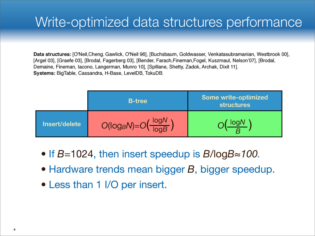
54. Don’t Thrash: How to Cache Your Hash in Flash Write-optimized data structures performance • If B=1024, then insert speedup is B/logB≈100. • Hardware trends mean bigger B, bigger speedup. • Less than 1 I/O per insert. B-tree Some write-optimized structures Insert/delete O(logBN)=O( ) O( ) logN logB logN B Data structures: [O'Neil,Cheng, Gawlick, O'Neil 96], [Buchsbaum, Goldwasser, Venkatasubramanian, Westbrook 00], [Argel 03], [Graefe 03], [Brodal, Fagerberg 03], [Bender, Farach,Fineman,Fogel, Kuszmaul, Nelson’07], [Brodal, Demaine, Fineman, Iacono, Langerman, Munro 10], [Spillane, Shetty, Zadok, Archak, Dixit 11]. Systems: BigTable, Cassandra, H-Base, LevelDB, TokuDB. 9
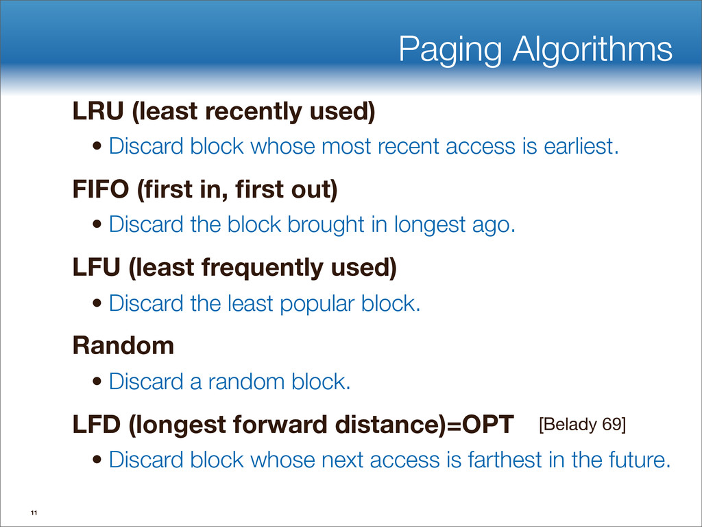
55. Don’t Thrash: How to Cache Your Hash in Flash Optimal Search-Insert Tradeoff [Brodal, Fagerberg 03] insert point query Optimal tradeoff (function of ɛ=0...1) B-tree (ɛ=1) O ✓ logB N p B ◆ O (logB N ) O (logB N ) ɛ=1/2 O ✓ log N B ◆ O (log N ) ɛ=0 O log1+B" N O ✓ log1+B" N B1 " ◆ O (logB N ) 10x-100x faster inserts 10
56. Don’t Thrash: How to Cache Your Hash in Flash Illustration of Optimal Tradeoff [Brodal, Fagerberg 03] Inserts Point Queries Fast Slow Slow Fast B-tree Logging Optimal Curve 11
57. Don’t Thrash: How to Cache Your Hash in Flash Illustration of Optimal Tradeoff [Brodal, Fagerberg 03] Inserts Point Queries Fast Slow Slow Fast B-tree Logging Optimal Curve Insertions improve by 10x-100x with almost no loss of point- query performance Target of opportunity 12
58. Don’t Thrash: How to Cache Your Hash in Flash Illustration of Optimal Tradeoff [Brodal, Fagerberg 03] Inserts Point Queries Fast Slow Slow Fast B-tree Logging Optimal Curve Insertions improve by 10x-100x with almost no loss of point- query performance Target of opportunity 12
59. One way to Build Write- Optimized Structures (Other approaches later)
60. Don’t Thrash: How to Cache Your Hash in Flash A simple write-optimized structure O(log N) queries and O((log N)/B) inserts: • A balanced binary tree with buffers of size B Inserts + deletes: • Send insert/delete messages down from the root and store them in buffers. • When a buffer fills up, flush. 14
61. Don’t Thrash: How to Cache Your Hash in Flash A simple write-optimized structure O(log N) queries and O((log N)/B) inserts: • A balanced binary tree with buffers of size B Inserts + deletes: • Send insert/delete messages down from the root and store them in buffers. • When a buffer fills up, flush. 14
62. Don’t Thrash: How to Cache Your Hash in Flash A simple write-optimized structure O(log N) queries and O((log N)/B) inserts: • A balanced binary tree with buffers of size B Inserts + deletes: • Send insert/delete messages down from the root and store them in buffers. • When a buffer fills up, flush. 14
63. Don’t Thrash: How to Cache Your Hash in Flash A simple write-optimized structure O(log N) queries and O((log N)/B) inserts: • A balanced binary tree with buffers of size B Inserts + deletes: • Send insert/delete messages down from the root and store them in buffers. • When a buffer fills up, flush. 14
64. Don’t Thrash: How to Cache Your Hash in Flash A simple write-optimized structure O(log N) queries and O((log N)/B) inserts: • A balanced binary tree with buffers of size B Inserts + deletes: • Send insert/delete messages down from the root and store them in buffers. • When a buffer fills up, flush. 14
65. Don’t Thrash: How to Cache Your Hash in Flash A simple write-optimized structure O(log N) queries and O((log N)/B) inserts: • A balanced binary tree with buffers of size B Inserts + deletes: • Send insert/delete messages down from the root and store them in buffers. • When a buffer fills up, flush. 15
66. Don’t Thrash: How to Cache Your Hash in Flash Analysis of writes An insert/delete costs amortized O((log N)/B) per insert or delete • A buffer flush costs O(1) & sends B elements down one level • It costs O(1/B) to send element down one level of the tree. • There are O(log N) levels in a tree. 16
67. Difficulty of Key Accesses
68. Difficulty of Key Accesses
69. Don’t Thrash: How to Cache Your Hash in Flash Analysis of point queries To search: • examine each buffer along a single root-to-leaf path. • This costs O(log N). 18
70. Don’t Thrash: How to Cache Your Hash in Flash Obtaining optimal point queries + very fast inserts Point queries cost O(log√B N)= O(logB N) • This is the tree height. Inserts cost O((logBN)/√B) • Each flush cost O(1) I/Os and flushes √B elements. √B B ... fanout: √B 19
71. Don’t Thrash: How to Cache Your Hash in Flash Cache-oblivious write-optimized structures You can even make these data structures cache-oblivious. This means that the data structure can be made platform independent (no knobs), i.e., works simultaneously for all values of B and M. [Bender, Farach-Colton, Fineman, Fogel, Kuszmaul, Nelson, SPAA 07] [Brodal, Demaine, Fineman, Iacono, Langerman, Munro, SODA 10] Random accesses are expensive. You can be cache- and I/O-efficient with no knobs or other memory-hierarchy parameterization.
72. Don’t Thrash: How to Cache Your Hash in Flash Cache-oblivious write-optimized structures You can even make these data structures cache-oblivious. This means that the data structure can be made platform independent (no knobs), i.e., works simultaneously for all values of B and M. [Bender, Farach-Colton, Fineman, Fogel, Kuszmaul, Nelson, SPAA 07] [Brodal, Demaine, Fineman, Iacono, Langerman, Munro, SODA 10] Random accesses are expensive. You can be cache- and I/O-efficient with no knobs or other memory-hierarchy parameterization.
73. Don’t Thrash: How to Cache Your Hash in Flash What the world looks like Insert/point query asymmetry • Inserts can be fast: >50K high-entropy writes/sec/disk. • Point queries are necessarily slow: <200 high-entropy reads/ sec/disk. We are used to reads and writes having about the same cost, but writing is easier than reading. Reading is hard. Writing is easier. 21
74. Don’t Thrash: How to Cache Your Hash in Flash The right read-optimization is write-optimization The right index makes queries run fast. • Write-optimized structures maintain indexes efficiently. data indexing query processor queries ??? 42 answers data ingestion 22
75. Don’t Thrash: How to Cache Your Hash in Flash The right read-optimization is write-optimization The right index makes queries run fast. • Write-optimized structures maintain indexes efficiently. Fast writing is a currency we use to accelerate queries. Better indexing means faster queries. data indexing query processor queries ??? 42 answers data ingestion 22
76. Don’t Thrash: How to Cache Your Hash in Flash The right read-optimization is write-optimization I/O Load Add selective indexes. (We can now afford to maintain them.) 23
77. Don’t Thrash: How to Cache Your Hash in Flash The right read-optimization is write-optimization I/O Load Add selective indexes. (We can now afford to maintain them.) Write-optimized structures can significantly mitigate the insert/query/freshness tradeoff. 3 23
78. Implementation Issues
79. Don’t Thrash: How to Cache Your Hash in Flash Write optimization. ✔ What’s missing? Optimal read-write tradeoff: Easy Full featured: Hard • Variable-sized rows • Concurrency-control mechanisms • Multithreading • Transactions, logging, ACID-compliant crash recovery • Optimizations for the special cases of sequential inserts and bulk loads • Compression • Backup 25
80. Don’t Thrash: How to Cache Your Hash in Flash Systems often assume search cost = insert cost Some inserts/deletes have hidden searches. Example: • return error when a duplicate key is inserted. • return # elements removed on a delete. These “cryptosearches” throttle insertions down to the performance of B-trees. 26
81. Don’t Thrash: How to Cache Your Hash in Flash Cryptosearches in uniqueness checking Uniqueness checking has a hidden search: In a B-tree uniqueness checking comes for free • On insert, you fetch a leaf. • Checking if key exists is no biggie. If Search(key) == True Return Error; Else Fast_Insert(key,value);
82. Don’t Thrash: How to Cache Your Hash in Flash Cryptosearches in uniqueness checking Uniqueness checking has a hidden search: In a write-optimized structure, that crypto- search can throttle performance • Insertion messages are injected. • These eventually get to “bottom” of structure. • Insertion w/Uniqueness Checking 100x slower. • Bloom filters, Cascade Filters, etc help. If Search(key) == True Return Error; Else Fast_Insert(key,value); [Bender, Farach-Colton, Johnson, Kraner, Kuszmaul, Medjedovic, Montes, Shetty, Spillane, Zadok 12] 28
83. Don’t Thrash: How to Cache Your Hash in Flash A simple implementation of pessimistic locking: maintain locks in leaves • Insert row t • Search for row u • Search for row v and put a cursor • Increment cursor. Now cursor points to row w. This scheme is inefficient for write-optimized structures because there are cryptosearches on writes. 29 v w t writer lock u reader lock reader range lock A locking scheme with cryptosearches
84. Performance
85. Don’t Thrash: How to Cache Your Hash in Flash iiBench Insertion Benchmark 31 nsertion of 1 billion rows into a table while maintaining three multicolumn second t the end of the test, TokuDB’s insertion rate remained at 17,028 inserts/second d dropped to 1,050 inserts/second. That’s a difference of over 16x. Ubuntu 10.10; 2x Xeon X5460; 16GB RAM; 8x 146GB 10k SAS in RAID10.
86. Don’t Thrash: How to Cache Your Hash in Flash Compression 32
87. Don’t Thrash: How to Cache Your Hash in Flash iiBench on SSD TokuDB on rotating disk beats InnoDB on SSD. 33 0 5000 10000 15000 20000 25000 30000 35000 0 5e+07 1e+08 1.5e+08 Insertion Rate Cummulative Insertions RAID10 X25-E FusionIO InnoDB TokuDB RAID10 X25E FusionIO
88. Don’t Thrash: How to Cache Your Hash in Flash Write-optimization Can Help Schema Changes 34 wntime is seconds to minutes. We detailed an experiment that showed this in 0 also introduced Hot Indexing. You can add an index to an existing table with The total downtime is seconds to a few minutes, because when the index is fin L closes and reopens the table. This means that the downtime occurs not when issued, but later on. Still, it is quite minimal, as we showed in this blog. ntOS 5.5; 2x Xeon E5310; 4GB RAM; 4x 1TB 7.2k SATA in RAID0. – Software Configuration Details back to top
89. Don’t Thrash: How to Cache Your Hash in Flash MongoDB with Fractal-Tree Index 35 !
90. Scaling into the Future
91. Don’t Thrash: How to Cache Your Hash in Flash Write-optimization going forward Example: Time to fill a disk in 1973, 2010, 2022. • log high-entropy data sequentially versus index data in B-tree. Better data structures may be a luxury now, but they will be essential by the decade’s end. Year Size Bandwidth Access Time Time to log data on disk Time to fill disk using a B-tree (row size 1K) 1973 35MB 835KB/s 25ms 39s 975s 2010 3TB 150MB/s 10ms 5.5h 347d 2022 220TB 1.05GB/s 10ms 2.4d 70y
92. Don’t Thrash: How to Cache Your Hash in Flash Write-optimization going forward Example: Time to fill a disk in 1973, 2010, 2022. • log high-entropy data sequentially versus index data in B-tree. Better data structures may be a luxury now, but they will be essential by the decade’s end. Year Size Bandwidth Access Time Time to log data on disk Time to fill disk using a B-tree (row size 1K) Time to fill using Fractal tree* (row size 1K) 1973 35MB 835KB/s 25ms 39s 975s 2010 3TB 150MB/s 10ms 5.5h 347d 2022 220TB 1.05GB/s 10ms 2.4d 70y * Projected times for fully multi-threaded version 38
93. Don’t Thrash: How to Cache Your Hash in Flash Write-optimization going forward Example: Time to fill a disk in 1973, 2010, 2022. • log high-entropy data sequentially versus index data in B-tree. Better data structures may be a luxury now, but they will be essential by the decade’s end. Year Size Bandwidth Access Time Time to log data on disk Time to fill disk using a B-tree (row size 1K) Time to fill using Fractal tree* (row size 1K) 1973 35MB 835KB/s 25ms 39s 975s 200s 2010 3TB 150MB/s 10ms 5.5h 347d 36h 2022 220TB 1.05GB/s 10ms 2.4d 70y 23.3d * Projected times for fully multi-threaded version 39
94. Don’t Thrash: How to Cache Your Hash in Flash Summary of Module Write-optimization can solve many problems. • There is a provable point-query insert tradeoff. We can insert 10x-100x faster without hurting point queries. • We can avoid much of the funny tradeoff between data ingestion, freshness, and query speed. • We can avoid tuning knobs. write-optimized
95. Data Structures and Algorithms for Big Data Module 3: (Case Study) TokuFS--How to Make a Write- Optimized File System Michael A. Bender Stony Brook & Tokutek Bradley C. Kuszmaul MIT & Tokutek
96. Don’t Thrash: How to Cache Your Hash in Flash Story for Module Algorithms for Big Data apply to all storage systems, not just databases. Some big-data users store use a file system. The problem with Big Data is Microdata... 2
97. HEC FSIO Grand Challenges Store 1 trillion files Create tens of thousands of files per second Traverse directory hierarchies fast (ls -R) B-trees would require at least hundreds of disk drives.
98. Don’t Thrash: How to Cache Your Hash in Flash TokuFS TokuFS • A file-system prototype • >20K file creates/sec • very fast ls -R • HEC grand challenges on a cheap disk (except 1 trillion files) [Esmet, Bender, Farach-Colton, Kuszmaul HotStorage12] TokuFS TokuDB XFS
99. Don’t Thrash: How to Cache Your Hash in Flash TokuFS TokuFS • A file-system prototype • >20K file creates/sec • very fast ls -R • HEC grand challenges on a cheap disk (except 1 trillion files) • TokuFS offers orders-of-magnitude speedup on microdata workloads. ‣ Aggregates microwrites while indexing. ‣ So it can be faster than the underlying file system. [Esmet, Bender, Farach-Colton, Kuszmaul HotStorage12] TokuFS TokuDB XFS
100. Don’t Thrash: How to Cache Your Hash in Flash Big speedups on microwrites We ran microdata-intensive benchmarks • Compared TokuFS to ext4, XFS, Btrfs, ZFS. • Stressed metadata and file data. • Used commodity hardware: ‣2 core AMD, 4GB RAM ‣Single 7200 RPM disk ‣Simple, cheap setup. No hardware tricks. • In all tests, we observed orders of magnitude speed up. 6
101. Don’t Thrash: How to Cache Your Hash in Flash Create 2 million 200-byte files in a shallow tree Faster on small file creation 7
102. Don’t Thrash: How to Cache Your Hash in Flash Create 2 million 200-byte files in a shallow tree Faster on small file creation Log scale 7
103. Don’t Thrash: How to Cache Your Hash in Flash Faster on metadata scan Recursively scan directory tree for metadata • Use the same 2 million files created before. • Start on a cold cache to measure disk I/O efficiency 8
104. Don’t Thrash: How to Cache Your Hash in Flash Faster on big directories Create one million empty files in a directory • Create files with random names, then read them back. • Tests how well a single directory scales. 9
105. Don’t Thrash: How to Cache Your Hash in Flash Faster on microwrites in a big file Randomly write out a file in small, unaligned pieces 10
106. TokuFS Implementation
107. Don’t Thrash: How to Cache Your Hash in Flash TokuFS employs two indexes Metadata index: • The metadata index maps pathname to file metadata. ‣/home/esmet ⟹ mode, file size, access times, ... ‣/home/esmet/tokufs.c ⟹ mode, file size, access times, ... Data index: • The data index maps pathname, blocknum to bytes. ‣/home/esmet/tokufs.c, 0 ⟹ [ block of bytes ] ‣/home/esmet/tokufs.c, 1 ⟹ [ block of bytes ] • Block size is a compile-time constant: 512. ‣ good performance on small files, moderate on large files 12
108. Don’t Thrash: How to Cache Your Hash in Flash Common queries exhibit locality Metadata index keys: full path as string • All the children of a directory are contiguous in the index • Reading a directory is simple and fast Data block index keys:ʲfull path, blocknumʳ • So all the blocks for a file are contiguous in the index • Reading a file is simple and fast 13
109. Don’t Thrash: How to Cache Your Hash in Flash TokuFS compresses indexes Reduces overhead from full path keys • Pathnames are highly “prefix redundant” • They compress very, very well in practice Reduces overhead from zero-valued padding • Uninitialized bytes in a block are set to zero • Good portions of the metadata struct are set to zero Compression between 7-15x on real data • For example, a full MySQL source tree 14
110. Don’t Thrash: How to Cache Your Hash in Flash TokuFS is fully functional TokuFS is a prototype, but fully functional. • Implements files, directories, metadata, etc. • Interfaces with applications via shared library, header. We wrote a FUSE implementation, too. • FUSE lets you implement filesystems in user space. • But there’s overhead, so performance isn’t optimal. • The best way to run is through our POSIX-like file API. 15
111. Microdata is the Problem
112. Data Structures and Algorithms for Big Data Module 4: Paging Michael A. Bender Stony Brook & Tokutek Bradley C. Kuszmaul MIT & Tokutek
113. This Module 2 The algorithmics of cache-management. This will help us understand I/O- and cache-efficient algorithms.
114. Goal: minimize # block transfers. • Data is transferred in blocks between RAM and disk. • Performance bounds are parameterized by B, M, N. When a block is cached, the access cost is 0. Otherwise it’s 1. Recall Disk Access Model Disk RAM B M 3 [Aggarwal+Vitter ’88]
115. Disk Access Model (DAM Model): • Performance bounds are parameterized by B, M, N. Goal: Minimize # of block transfers. Beautiful restriction: • Parameters B, M are unknown to the algorithm or coder. Recall Cache-Oblivious Analysis Disk RAM B=?? M=?? 4 [Frigo, Leiserson, Prokop, Ramachandran ’99]
116. CO analysis applies to unknown multilevel hierarchies: • Cache-oblivious algorithms work for all B and M... • ... and all levels of a multi-level hierarchy. Moral: • It’s better to optimize approximately for all B, M rather than to try to pick the best B and M. Recall Cache-Oblivious Analysis Disk RAM B=?? M=?? 5 [Frigo, Leiserson, Prokop, Ramachandran ’99]
117. Cache-Replacement in Cache-Oblivious Algorithms Which blocks are currently cached in RAM? • The system performs its own caching/paging. • If we knew B and M we could explicitly manage I/O. (But even then, what should we do?) 6 Disk RAM B=?? M=??
118. Cache-Replacement in Cache-Oblivious Algorithms Which blocks are currently cached in RAM? • The system performs its own caching/paging. • If we knew B and M we could explicitly manage I/O. (But even then, what should we do?) But systems may use different mechanisms, so what can we actually assume? 6 Disk RAM B=?? M=??
119. This Module: Cache-Management Strategies With cache-oblivious analysis, we can assume a memory system with optimal replacement. Even though the system manages memory, we can assume all the advantages of explicit memory management. 7 Disk RAM B=?? M=??
120. This Module: Cache-Management Strategies An LRU-based system with memory M performs cache-management < 2x worse than the optimal, prescient policy with memory M/2. Achieving optimal cache-management is hard because predicting the future is hard. But LRU with (1+ɛ)M memory is almost as good (or better), than the optimal strategy with M memory. 8 Disk OPT M [Sleator, Tarjan 85] Disk LRU (1+ɛ) M LRU with (1+ɛ) more memory is nearly as good or better... ... than OPT.
121. The paging/caching problem A program is just sequence of block requests: Cost of request rj Algorithmic question: • Which block should be ejected when block rj is brought into cache? 9 r1, r2, r3, . . . cost( rj) = ⇢ 0 block rj is already cached, 1 block rj is brought into cache.
122. The paging/caching problem RAM holds only k=M/B blocks. Which block should be ejected when block rj is brought into cache? 10 Disk RAM M rj ???
123. Paging Algorithms LRU (least recently used) • Discard block whose most recent access is earliest. FIFO (first in, first out) • Discard the block brought in longest ago. LFU (least frequently used) • Discard the least popular block. Random • Discard a random block. LFD (longest forward distance)=OPT • Discard block whose next access is farthest in the future. 11 [Belady 69]
124. LFD (Longest Forward Distance) [Belady ’69]: • Discard the block requested farthest in the future. Cons: Who knows the Future?! Pros: LFD can be viewed as a point of comparison with online strategies. 12 Page 5348 shall be requested tomorrow at 2:00 pm Optimal Page Replacement
125. LFD (Longest Forward Distance) [Belady ’69]: • Discard the block requested farthest in the future. Cons: Who knows the Future?! Pros: LFD can be viewed as a point of comparison with online strategies. 13 Page 5348 shall be requested tomorrow at 2:00 pm Optimal Page Replacement
126. LFD (Longest Forward Distance) [Belady ’69]: • Discard the block requested farthest in the future. Cons: Who knows the Future?! Pros: LFD can be viewed as a point of comparison with online strategies. 14 Page 5348 shall be requested tomorrow at 2:00 pm Optimal Page Replacement
127. Competitive Analysis An online algorithm A is k-competitive, if for every request sequence R: Idea of competitive analysis: • The optimal (prescient) algorithm is a yardstick we use to compare online algorithms. 15 costA( R )  k costopt( R )
128. LRU is no better than k-competitive Memory holds 3 blocks The program accesses 4 different blocks The request stream is 16 M M/B = k = 3 rj 2 {1, 2, 3, 4} 1, 2, 3, 4, 1, 2, 3, 4, · · ·
129. LRU is no better than k-competitive 17 requests blocks in memory There’s a block transfer at every step because LRU ejects the block that’s requested in the next step. 1 2 3 4 1 2 3 4 1 2 1 1 1 1 1 1 1 1 2 2 2 2 2 2 2 3 3 3 3 3 3 4 4 4 4 4 4
130. LRU is no better than k-competitive 18 requests blocks in memory LFD (longest forward distance) has a block transfer every k=3 steps. 1 2 3 4 1 2 3 4 1 2 1 1 1 1 1 1 1 1 1 1 2 2 2 2 2 2 3 3 3 3 3 4 4 4 4 4 4 4
131. LRU is k-competitive In fact, LRU is k=M/B-competitive. • I.e., LRU has k=M/B times more transfers than OPT. • A depressing result because k is huge so k . OPT is nothing to write home about. LFU and FIFO are also k-competitive. • This is a depressing result because FIFO is empirically worse than LRU, and this isn’t captured in the math. 19 [Sleator, Tarjan 85]
132. On the other hand, the LRU bad example is fragile 20 requests blocks in memory If k=M/B=4, not 3, then both LRU and OPT do well. If k=M/B=2, not 3, then neither LRU nor OPT does well. 1 2 3 4 1 2 3 4 1 2 1 1 1 1 1 1 1 1 2 2 2 2 2 2 2 3 3 3 3 3 3 4 4 4 4 4 4
133. LRU is 2-competitive with more memory LRU is at most twice as bad as OPT, when LRU has twice the memory. In general, LRU is nearly as good as OPT when LRU has a little more memory than OPT. 21 LRU|cache|=k (R)  2 OPT|cache|=k/2 (R) [Sleator, Tarjan 85]
134. LRU is 2-competitive with more memory LRU is at most twice as bad as OPT, when LRU has twice the memory. In general, LRU is nearly as good as OPT when LRU has a little more memory than OPT. 21 LRU|cache|=k (R)  2 OPT|cache|=k/2 (R) [Sleator, Tarjan 85] LRU has more memory, but OPT=LFD can see the future.
135. LRU is 2-competitive with more memory LRU is at most twice as bad as OPT, when LRU has twice the memory. In general, LRU is nearly as good as OPT when LRU has a little more memory than OPT. 21 LRU|cache|=k (R)  2 OPT|cache|=k/2 (R) [Sleator, Tarjan 85] LRU has more memory, but OPT=LFD can see the future.
136. LRU is 2-competitive with more memory LRU is at most twice as bad as OPT, when LRU has twice the memory. In general, LRU is nearly as good as OPT when LRU has a little more memory than OPT. 21 LRU|cache|=k (R)  2 OPT|cache|=k/2 (R) [Sleator, Tarjan 85] (These bounds don’t apply to FIFO, distinguishing LRU from FIFO). LRU has more memory, but OPT=LFD can see the future.
137. Divide LRU into phases, each with k faults. LRU Performance Proof 22 r1, r2, . . . , ri, ri+1, . . . , rj, rj+1, . . . , r`, r`+1, . . .
138. Divide LRU into phases, each with k faults. OPT[k] must have ≥ 1 fault in each phase. • Case analysis proof. • LRU is k-competitive. LRU Performance Proof 22 r1, r2, . . . , ri, ri+1, . . . , rj, rj+1, . . . , r`, r`+1, . . .
139. Divide LRU into phases, each with k faults. OPT[k] must have ≥ 1 fault in each phase. • Case analysis proof. • LRU is k-competitive. OPT[k/2] must have ≥ k/2 faults in each phase. • Main idea: each phase must touch k different pages. • LRU is 2-competitive. LRU Performance Proof 22 r1, r2, . . . , ri, ri+1, . . . , rj, rj+1, . . . , r`, r`+1, . . .
140. Under the hood of cache-oblivious analysis Moral: with cache-oblivious analysis, we can analyze based on a memory system with optimal, omniscient replacement. • Technically, an optimal cache-oblivious algorithm is asymptotically optimal versus any algorithm on a memory system that is slightly smaller. • Empirically, this is just a technicality. 23 Disk OPT M Disk LRU (1+ɛ) M This is almost as good or better... ... than this.
141. Ramifications for New Cache-Replacement Policies Moral: There’s not much performance on the table for new cache-replacement policies. • Bad instances for LRU versus LFD are fragile and very sensitive to k=M/B. There are still research questions: • What if blocks have different sizes [Irani 02][Young 02]? • There’s a write-back cost? (Complexity unknown.) • LRU may be too costly to implement (clock algorithm). 24
142. Data Structures and Algorithms for Big Data Module 5: What to Index Michael A. Bender Stony Brook & Tokutek Bradley C. Kuszmaul MIT & Tokutek
143. Don’t Thrash: How to Cache Your Hash in Flash Story of this module This module explores indexing. Traditionally, (with B-trees), indexing speeds queries, but cripples insert. But now we know that maintaining indexes is cheap. So what should you index? 2
144. Don’t Thrash: How to Cache Your Hash in Flash An Indexing Testimonial This is a graph from a real user, who added some indexes, and reduced the I/O load on their server. (They couldn’t maintain the indexes with B-trees.) 3 I/O Load Add selective indexes.
145. What is an Index? To understand what to index, we need to get on the same page for what an index is.
146. Row, Index, and Table Row • Key,value pair • key = a, value = b,c Index • Ordering of rows by key (dictionary) • Used to make queries fast Table • Set of indexes a b c 100 5 45 101 92 2 156 56 45 165 6 2 198 202 56 206 23 252 256 56 2 412 43 45 create table foo (a int, b int, c int, primary key(a));
147. An index is a dictionary Dictionary API: maintain a set S subject to • insert(x): S ← S ∪ {x} • delete(x): S ← S - {x} • search(x): is x ∊ S? • successor(x): return min y > x s.t. y ∊ S • predecessor(y): return max y < x s.t. y ∊ S We assume that these operations perform as well as a B-tree. For example, the successor operation usually doesn’t require an I/O.
148. A table is a set of indexes A table is a set of indexes with operations: • Add index: add key(f1,f2,...); • Drop index: drop key(f1,f2,...); • Add column: adds a field to primary key value. • Remove column: removes a field and drops all indexes where field is part of key. • Change field type • ... Subject to index correctness constraints. We want table operations to be fast too.
149. Next: how to use indexes to improve queries.
150. Indexes provide query performance 1. Indexes can reduce the amount of retrieved data. • Less bandwidth, less processing, ... 2. Indexes can improve locality. • Not all data access cost is the same • Sequential access is MUCH faster than random access 3. Indexes can presort data. • GROUP BY and ORDER BY queries do post-retrieval work • Indexing can help get rid of this work
151. Indexes provide query performance 1. Indexes can reduce the amount of retrieved data. • Less bandwidth, less processing, ... 2. Indexes can improve locality. • Not all data access cost is the same • Sequential access is MUCH faster than random access 3. Indexes can presort data. • GROUP BY and ORDER BY queries do post-retrieval work • Indexing can help get rid of this work
152. a b c 100 5 45 101 92 2 156 56 45 165 6 2 198 202 56 206 23 252 256 56 2 412 43 45 An index can select needed rows count (*) where a<120;
153. a b c 100 5 45 101 92 2 156 56 45 165 6 2 198 202 56 206 23 252 256 56 2 412 43 45 100 5 45 101 92 2 An index can select needed rows 100 5 45 101 92 2 2 } count (*) where a<120;
154. No good index means slow table scans a b c 100 5 45 101 92 2 156 56 45 165 6 2 198 202 56 206 23 252 256 56 2 412 43 45 count (*) where b>50 and b<100;
155. No good index means slow table scans a b c 100 5 45 101 92 2 156 56 45 165 6 2 198 202 56 206 23 252 256 56 2 412 43 45 count (*) where b>50 and b<100; 100 5 45 101 92 2 156 56 45 165 6 2 198 202 56 206 23 252 256 56 2 412 43 45 101 92 2 156 56 45 256 56 2 0 1 2 3
156. You can add an index a b c 100 5 45 101 92 2 156 56 45 165 6 2 198 202 56 206 23 252 256 56 2 412 43 45 alter table foo add key(b); b a 5 100 6 165 23 206 43 412 56 156 56 256 92 101 202 198
157. A selective index speeds up queries a b c 100 5 45 101 92 2 156 56 45 165 6 2 198 202 56 206 23 252 256 56 2 412 43 45 count (*) where b>50 and b<100; b a 5 100 6 165 23 206 43 412 56 156 56 256 92 101 202 198
158. A selective index speeds up queries a b c 100 5 45 101 92 2 156 56 45 165 6 2 198 202 56 206 23 252 256 56 2 412 43 45 count (*) where b>50 and b<100; b a 5 100 6 165 23 206 43 412 56 156 56 256 92 101 202 198 3 } 56 156 56 256 92 101 56 156 56 256 92 101
159. b a 5 100 6 165 23 206 43 412 56 156 56 256 92 101 202 198 a b c 100 5 45 101 92 2 156 56 45 165 6 2 198 202 56 206 23 252 256 56 2 412 43 45 Selective indexes can still be slow sum(c) where b>50;
160. b a 5 100 6 165 23 206 43 412 56 156 56 256 92 101 202 198 56 156 56 256 92 101 202 198 a b c 100 5 45 101 92 2 156 56 45 165 6 2 198 202 56 206 23 252 256 56 2 412 43 45 Selective indexes can still be slow 56 156 56 256 92 101 202 198 Selecting on b: fast sum(c) where b>50;
161. b a 5 100 6 165 23 206 43 412 56 156 56 256 92 101 202 198 56 156 56 256 92 101 202 198 a b c 100 5 45 101 92 2 156 56 45 165 6 2 198 202 56 206 23 252 256 56 2 412 43 45 Selective indexes can still be slow 56 156 56 256 92 101 202 198 Fetching info for summing c: slow Selecting on b: fast sum(c) where b>50; 156
162. b a 5 100 6 165 23 206 43 412 56 156 56 256 92 101 202 198 56 156 56 256 92 101 202 198 a b c 100 5 45 101 92 2 156 56 45 165 6 2 198 202 56 206 23 252 256 56 2 412 43 45 156 56 45 Selective indexes can still be slow 56 156 56 256 92 101 202 198 156 56 45 Fetching info for summing c: slow Selecting on b: fast sum(c) where b>50;
163. b a 5 100 6 165 23 206 43 412 56 156 56 256 92 101 202 198 56 156 56 256 92 101 202 198 a b c 100 5 45 101 92 2 156 56 45 165 6 2 198 202 56 206 23 252 256 56 2 412 43 45 156 56 45 Selective indexes can still be slow 56 156 56 256 92 101 202 198 156 56 45 Fetching info for summing c: slow Selecting on b: fast sum(c) where b>50; 256
164. b a 5 100 6 165 23 206 43 412 56 156 56 256 92 101 202 198 56 156 56 256 92 101 202 198 a b c 100 5 45 101 92 2 156 56 45 165 6 2 198 202 56 206 23 252 256 56 2 412 43 45 256 56 2 156 56 45 Selective indexes can still be slow 56 156 56 256 92 101 202 198 156 56 45 256 56 2 Fetching info for summing c: slow Selecting on b: fast sum(c) where b>50;
165. b a 5 100 6 165 23 206 43 412 56 156 56 256 92 101 202 198 56 156 56 256 92 101 202 198 a b c 100 5 45 101 92 2 156 56 45 165 6 2 198 202 56 206 23 252 256 56 2 412 43 45 256 56 2 198 202 56 156 56 45 101 92 2 Selective indexes can still be slow 56 156 56 256 92 101 202 198 156 56 45 256 56 2 101 92 2 198 202 56 Fetching info for summing c: slow Selecting on b: fast sum(c) where b>50; 45 2 2 56 Poor data locality
166. b a 5 100 6 165 23 206 43 412 56 156 56 256 92 101 202 198 56 156 56 256 92 101 202 198 a b c 100 5 45 101 92 2 156 56 45 165 6 2 198 202 56 206 23 252 256 56 2 412 43 45 256 56 2 198 202 56 156 56 45 101 92 2 Selective indexes can still be slow 56 156 56 256 92 101 202 198 105 156 56 45 256 56 2 101 92 2 198 202 56 Fetching info for summing c: slow Selecting on b: fast sum(c) where b>50; 45 2 2 56 Poor data locality
167. Indexes provide query performance 1. Indexes can reduce the amount of retrieved data. • Less bandwidth, less processing, ... 2. Indexes can improve locality. • Not all data access cost is the same • Sequential access is MUCH faster than random access 3. Indexes can presort data. • GROUP BY and ORDER BY queries do post-retrieval work • Indexing can help get rid of this work
168. b,c a 5,45 100 6,2 165 23,252 206 43,45 412 56,2 256 56,45 156 92,2 101 202,56 198 Covering indexes speed up queries a b c 100 5 45 101 92 2 156 56 45 165 6 2 198 202 56 206 23 252 256 56 2 412 43 45 alter table foo add key(b,c); sum(c) where b>50;
169. b,c a 5,45 100 6,2 165 23,252 206 43,45 412 56,2 256 56,45 156 92,2 101 202,56 198 56,2 256 56,45 156 92,2 101 202,56 198 Covering indexes speed up queries a b c 100 5 45 101 92 2 156 56 45 165 6 2 198 202 56 206 23 252 256 56 2 412 43 45 56,2 256 56,45 156 92,2 101 202,56 198 105 alter table foo add key(b,c); sum(c) where b>50; 56,2 256 56,45 156 92,2 101 202,56 198
170. Indexes provide query performance 1. Indexes can reduce the amount of retrieved data. • Less bandwidth, less processing, ... 2. Indexes can improve locality. • Not all data access cost is the same • Sequential access is MUCH faster than random access 3. Indexes can presort data. • GROUP BY and ORDER BY queries do post-retrieval work • Indexing can help get rid of this work
171. b,c a 5,45 100 6,2 165 23,252 206 43,45 412 56,2 256 56,45 156 92,2 101 202,56 198 Indexes can avoid post-selection sorts a b c 100 5 45 101 92 2 156 56 45 165 6 2 198 202 56 206 23 252 256 56 2 412 43 45 select b, sum(c) group by b; sum(c) where b>50; b sum(c) 5 45 6 2 23 252 43 45 56 47 92 2 202 56
172. Data Structures and Algorithms for Big Data Module 6: Log Structured Merge Trees Michael A. Bender Stony Brook & Tokutek Bradley C. Kuszmaul MIT & Tokutek 1
173. Log Structured Merge Trees Log structured merge trees are write-optimized data structures developed in the 90s. Over the past 5 years, LSM trees have become popular (for good reason). Accumulo, Bigtable, bLSM, Cassandra, HBase, Hypertable, LevelDB are LSM trees (or borrow ideas). http://nosql-database.org lists 122 NoSQL databases. Many of them are LSM trees. 2 [O'Neil, Cheng, Gawlick, O'Neil 96]
174. Don’t Thrash: How to Cache Your Hash in Flash Recall Optimal Search-Insert Tradeoff [Brodal, Fagerberg 03] insert point query Optimal tradeoff (function of ɛ=0...1) O log1+B" N O ✓ log1+B" N B1 " ◆ 3 LSM trees don’t lie on the optimal search-insert tradeoff curve. But they’re not far off. We’ll show how to move them back onto the optimal curve.
175. Log Structured Merge Tree An LSM tree is a cascade of B-trees. Each tree Tj has a target size |Tj | . The target sizes are exponentially increasing. Typically, target size |Tj+1| = 10 |Tj |. 4 [O'Neil, Cheng, Gawlick, O'Neil 96] T0 T1 T2 T3 T4
176. LSM Tree Operations Point queries: 5 T0 T1 T2 T3 T4
177. LSM Tree Operations Point queries: Range queries: 5 T0 T1 T2 T3 T4 T0 T1 T2 T3 T4
178. LSM Tree Operations Insertions: • Always insert element into the smallest B-tree T0. • When a B-tree Tj fills up, flush into Tj+1 . 6 T0 T1 T2 T3 T4 T0 T1 T2 T3 T4 insert flush
179. LSM Tree Operations Deletes are like inserts: • Instead of deleting an element directly, insert tombstones. • A tombstone knocks out a “real” element when it lands in the same tree. 7 T0 T1 T2 T3 T4 T0 T1 T2 T3 T4 insert tombstone messages
180. Static-to-Dynamic Transformation An LSM Tree is an example of a “static-to- dynamic” transformation . • An LSM tree can be built out of static B-trees. • When T3 flushes into T4, T4 is rebuilt from scratch. 8 [Bentley, Saxe ’80] T0 T1 T2 T3 T4 flush
181. This Module 9 Let’s analyze LSM trees. B M
182. I/O models Recall: Searching in an Array Versus B-tree Recall the cost of searching in an array versus a B-tree. 10 O(logBN) O (logB N ) = O ✓ log2 N log2 B ◆
183. I/O models Recall: Searching in an Array Versus B-tree Recall the cost of searching in an array versus a B-tree. 10 O(logBN) O (logB N ) = O ✓ log2 N log2 B ◆ O ✓ log2 N B ◆ ⇡ O (log2 N )
184. Analysis of point queries Search cost: 11 T0 T1 T2 T3 T log N ... logB N + logB N/ 2 + logB N/ 4 + · · · + logB B = O (log N logB N ) = 1 log B (log N + log N 1 + log N 2 + log N 3 + · · · + 1)
185. Insert Analysis The cost to flush a tree Tj of size X is O(X/B). • Flushing and rebuilding a tree is just a linear scan. The cost per element to flush Tj is O(1/B). The # times each element is moved is ≤ log N. The insert cost is O((log N)/B) amortized memory transfers. 12 Tj has size X. A flush costs O(1/B) per element. Tj+1 has size ϴ(X).
186. Samples from LSM Tradeoff Curve sizes grow by B (ɛ=1) O ✓ logB N p B ◆ O (logB N ) O ✓ log N B ◆ sizes double (ɛ=0) O ✓ log1+B" N B1 " ◆ O (logB N )(log1+B" N ) point query tradeoff (function of ɛ) insert O ((logB N )(log N )) O ((logB N )(logB N )) O ((logB N )(logB N )) 13 sizes grow by B1/2 (ɛ=1/2)
187. How to improve LSM-tree point queries? Looking in all those trees is expensive, but can be improved by • caching, • Bloom filters, and • fractional cascading. 14 T0 T1 T2 T3 T4
188. Caching in LSM trees When the cache is warm, small trees are cached. 15 T0 T1 T2 T3 T4 When the cache is warm, these trees are cached.
189. Bloom filters in LSM trees Bloom filters can avoid point queries for elements that are not in a particular B-tree. We’ll see how Bloom filters work later. 16 T0 T1 T2 T3 T4
190. Fractional cascading reduces the cost in each tree Instead of avoiding searches in trees, we can use a technique called fractional cascading to reduce the cost of searching each B-tree to O(1). 17 T0 T1 T2 T3 T4 Idea: We’re looking for a key, and we already know where it should have been in T3, try to use that information to search T4.
191. Searching one tree helps in the next Looking up c, in Ti we know it’s between b, and e. 18 a c d f h i j k m n p q t u y z Ti+1 Ti b e v w Showing only the bottom level of each B-tree.
192. Forwarding pointers If we add forwarding pointers to the first tree, we can jump straight to the node in the second tree, to find c. 19 a c d f h i j k m n p q t u y z Ti+1 Ti b e v w
193. Remove redundant forwarding pointers We need only one forwarding pointer for each block in the next tree. Remove the redundant ones. 20 a c d f h i j k m n p q t u y z Ti+1 Ti b e v w
194. Ghost pointers We need a forwarding pointer for every block in the next tree, even if there are no corresponding pointers in this tree. Add ghosts. 21 a c d f h i j k m n p q t u y z Ti+1 Ti b e v w ghosts h m
195. LSM tree + forward + ghost = fast queries With forward pointers and ghosts, LSM trees require only one I/O per tree, and point queries cost only . 22 a c d f h i j k m n p q t u y z Ti+1 Ti b e v w ghosts h m [Bender, Farach-Colton, Fineman, Fogel, Kuszmaul, Nelson 07] O (logR N )
196. LSM tree + forward + ghost = COLA This data structure no longer uses the internal nodes of the B-trees, and each of the trees can be implemented by an array. 23 [Bender, Farach-Colton, Fineman, Fogel, Kuszmaul, Nelson 07] Ti+1 Ti b e v w m n p q h i j k t u y z a c d f ghosts h m Text
197. Data Structures and Algorithms for Big Data Module 7: Bloom Filters Michael A. Bender Stony Brook & Tokutek Bradley C. Kuszmaul MIT & Tokutek 1
198. Approximate Set Membership Problem We need a space-efficient in-memory data structure to represent a set S to which we can add elements. We want to answer membership queries approximately: • If x is in S then we want query(x,S) to return true. • Otherwise we want query(x,S) to usually return false. Bloom filters are a simple data structure to solve this problem. 2
199. How do approximate queries help? Recall for LSM trees (without fractional cascading), we wanted to avoid looking in a tree if we knew a key wasn’t there. Bloom filters allow us to usually avoid the lookup. 3 T0 T1 T2 T3 T4 Bloom filters don’t seem to help with range queries, however.
200. Simplified Bloom Filter Using hashing, but instead of storing elements we simply use one bit to keep track of whether an element is in the set. • Array A[m] bits. • Uniform hash function h: S --> [0,m). • To insert s: Set A[h(s)] = 1; • To check s: Check if A[h(s)]=1. 4
201. Example using Simplified Bloom Filter Use an array of length 6. Insert • insert a, where h(a)=3; • b, where h(b)=5. Look up • a: h(a)=3 Answer is yes. Maybe a is there. (And it is). • b: h(b)=5 Answer is yes. Maybe b is there. (And it is). • c: h(c)=2 Answer is no. Definitely c is not there. • d: h(d)=3 Answer is yes. Maybe d is there. (Nope.) 5 0 0 0 1 0 1 0 1 2 3 4 5
202. Analysis of Simplified Bloom Filter If n items are in an array of size m, then the chances of getting a YES answer on an element that is not there is . If you fill the array about 30% full, you get about a 50% odds of a false positive. Each object requires about 3 bits. How do you get the odds to be 1% false positive? 6 ⇡ 1 e n/m
203. Smaller False Positive One way would be to fill the array only 1% full. Not space efficient. Another way would be to use 7 arrays, with 7 hash functions. False positive rate becomes 1/128. Space is 21 bits per object. 7
204. Bloom filter Idea: Don’t use 7 separate arrays, use one array that’s 7 times bigger, and store the 7 hashed bits. For a 1% false positive rate, it takes about 10 bits per object. 8
205. Other Bloom Filters Counting bloom filters [Fan, Cao, Almeida, Broder 2000] allow deletions by maintaining a 4-bit counter instead of a single bit per object. Buffered Bloom Filters [Canin, Mihaila, Bhattacharhee, and Ross, 2010] employ hash localization to direct all the hashes of a single insertion to the same block. Cascade Filters [Bender, Farach-Colton, Johnson, Kraner, Kuszmaul, Medjedovic, Montes, Shetty, Spillane, Zadok 2011] support deletions, exhibit locality for queries, insert quickly, and are cache-oblivious. 9
206. Closing Words 10
207. We want to feel your pain. We are interested in hearing about other scaling problems. Come to talk to us. bender@cs.stonybrook.edu bradley@mit.edu 11
208. Big Data Epigrams The problem with big data is microdata. Sometimes the right read optimization is a write-optimization. As data becomes bigger, the asymptotics become more important. Life is too short for half-dry white-board markers and bad sushi. 12