Calibration with Neural Networks

Model Calibration with Neural Networks.
Presentation given at the July 2016 QuantLib User Conference in London

Transcript

1. Neural Networks Calibration Calibration with Neural Networks Example with Hull-White Andres Hernandez IBM Risk Analytics July 12, 2016 Andres Hernandez Calibration with Neural Networks
2. Neural Networks Calibration Motivation A central consideration of any pricing model is the ability to calibrate that model to market prices. Whether the necessary information, e.g. correlation, can be effectively implied from the data or not is one part of this, but also the speed with which that calibration can be done influences the usability of a model. Andres Hernandez Calibration with Neural Networks
3. Neural Networks Calibration Motivation The point of this talk is to provide a method that will perform the calibration significantly faster regardless of the model, hence removing the calibration speed from a model’s practicality. As an added benefit, but not addressed here, neural networks, as they are fully differentiable, could provide model parameters sensitivities to market prices, informing when a model should be recalibrated Andres Hernandez Calibration with Neural Networks
4. Neural Networks Calibration Table of contents 1 Neural Networks Introduction Universal approximation Training 2 Calibration Problem Example: Hull-White Neural Network Topology Results Andres Hernandez Calibration with Neural Networks
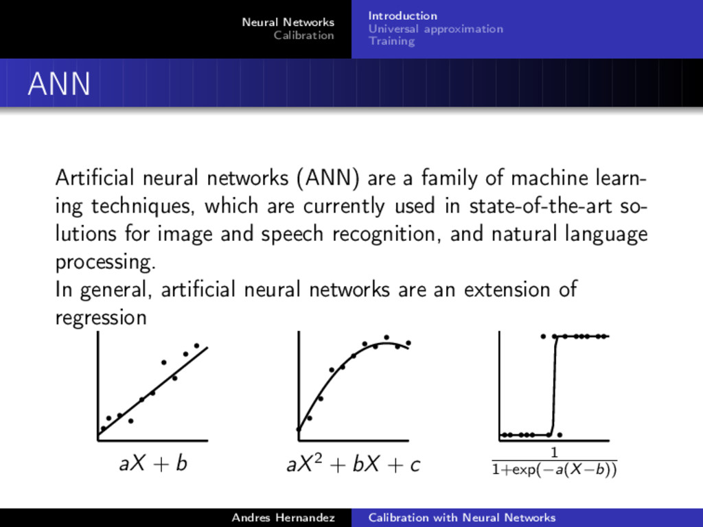
5. Neural Networks Calibration Introduction Universal approximation Training ANN Artificial neural networks (ANN) are a family of machine learn- ing techniques, which are currently used in state-of-the-art so- lutions for image and speech recognition, and natural language processing. In general, artificial neural networks are an extension of regression aX + b aX2 + bX + c 1 1+exp(−a(X−b)) Andres Hernandez Calibration with Neural Networks
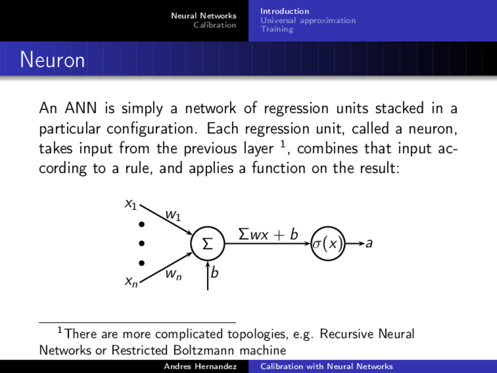
6. Neural Networks Calibration Introduction Universal approximation Training Neuron An ANN is simply a network of regression units stacked in a particular configuration. Each regression unit, called a neuron, takes input from the previous layer 1, combines that input ac- cording to a rule, and applies a function on the result: x1 w1 xn wn Σ b Σwx + b σ(x) a 1There are more complicated topologies, e.g. Recursive Neural Networks or Restricted Boltzmann machine Andres Hernandez Calibration with Neural Networks
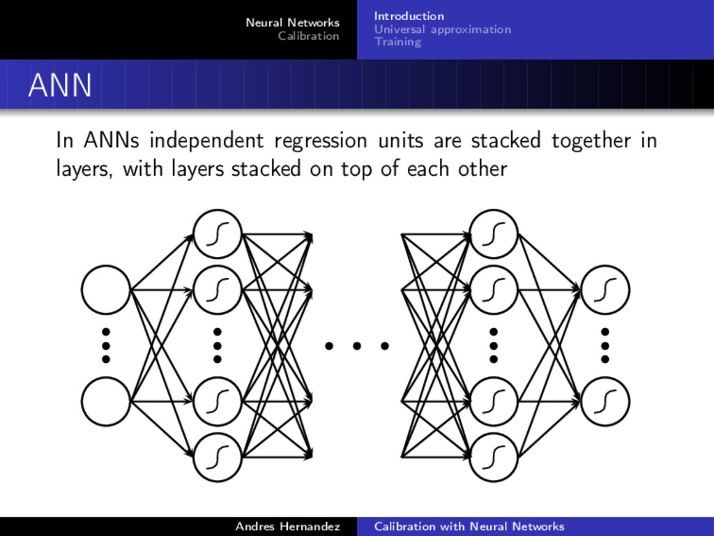
7. Neural Networks Calibration Introduction Universal approximation Training ANN In ANNs independent regression units are stacked together in layers, with layers stacked on top of each other Andres Hernandez Calibration with Neural Networks
8. Neural Networks Calibration Introduction Universal approximation Training Universal approximation theorem Neural networks are generally used to approximate a function, usually one with a large number of input parameters. To justify their use, besides practical results, one relies on the Universal Approximation theorem, which states that a continuous function in a compact domain can be arbitrarily approximated by a finite number of neurons with slight restrictions on the activation function. Andres Hernandez Calibration with Neural Networks
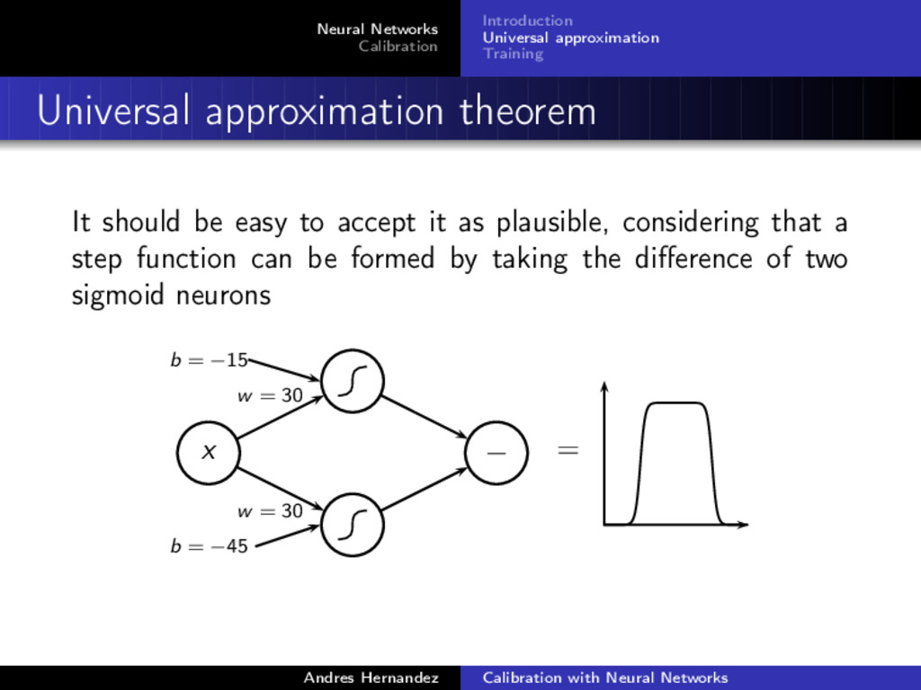
9. Neural Networks Calibration Introduction Universal approximation Training Universal approximation theorem It should be easy to accept it as plausible, considering that a step function can be formed by taking the difference of two sigmoid neurons x w = 30 b = −45 w = 30 b = −15 − = Andres Hernandez Calibration with Neural Networks
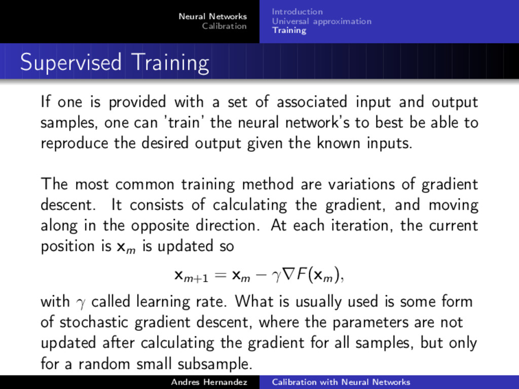
10. Neural Networks Calibration Introduction Universal approximation Training Supervised Training If one is provided with a set of associated input and output samples, one can ’train’ the neural network’s to best be able to reproduce the desired output given the known inputs. The most common training method are variations of gradient descent. It consists of calculating the gradient, and moving along in the opposite direction. At each iteration, the current position is xm is updated so xm+1 = xm − γ∇F(xm ), with γ called learning rate. What is usually used is some form of stochastic gradient descent, where the parameters are not updated after calculating the gradient for all samples, but only for a random small subsample. Andres Hernandez Calibration with Neural Networks
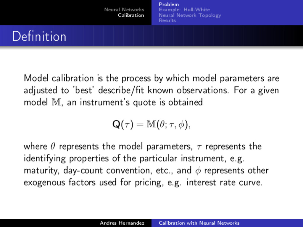
11. Neural Networks Calibration Problem Example: Hull-White Neural Network Topology Results Definition Model calibration is the process by which model parameters are adjusted to ’best’ describe/fit known observations. For a given model M, an instrument’s quote is obtained Q(τ) = M(θ; τ, φ), where θ represents the model parameters, τ represents the identifying properties of the particular instrument, e.g. maturity, day-count convention, etc., and φ represents other exogenous factors used for pricing, e.g. interest rate curve. Andres Hernandez Calibration with Neural Networks
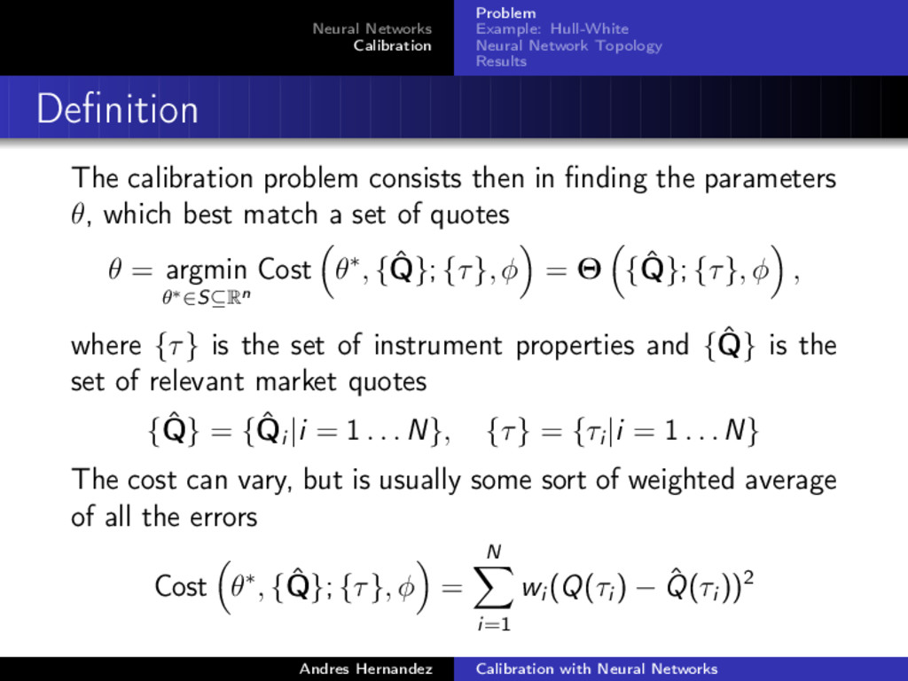
12. Neural Networks Calibration Problem Example: Hull-White Neural Network Topology Results Definition The calibration problem consists then in finding the parameters θ, which best match a set of quotes θ = argmin θ∗∈S⊆Rn Cost θ∗, { ˆ Q}; {τ}, φ = Θ { ˆ Q}; {τ}, φ , where {τ} is the set of instrument properties and { ˆ Q} is the set of relevant market quotes { ˆ Q} = { ˆ Qi |i = 1 . . . N}, {τ} = {τi |i = 1 . . . N} The cost can vary, but is usually some sort of weighted average of all the errors Cost θ∗, { ˆ Q}; {τ}, φ = N i=1 wi (Q(τi ) − ˆ Q(τi ))2 Andres Hernandez Calibration with Neural Networks
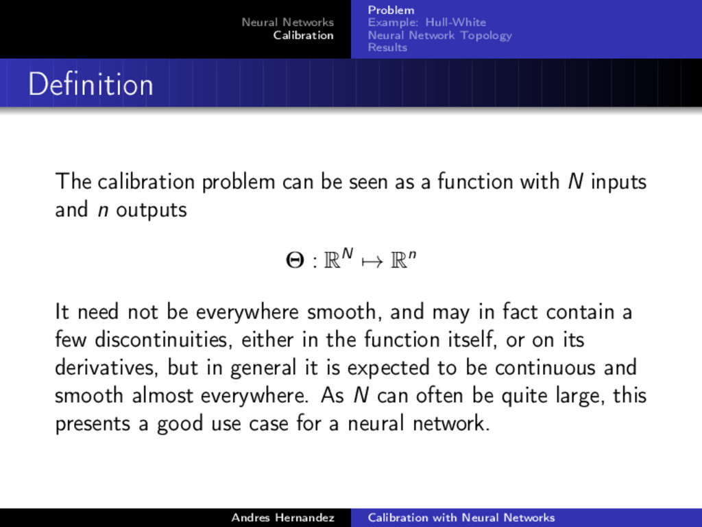
13. Neural Networks Calibration Problem Example: Hull-White Neural Network Topology Results Definition The calibration problem can be seen as a function with N inputs and n outputs Θ : RN → Rn It need not be everywhere smooth, and may in fact contain a few discontinuities, either in the function itself, or on its derivatives, but in general it is expected to be continuous and smooth almost everywhere. As N can often be quite large, this presents a good use case for a neural network. Andres Hernandez Calibration with Neural Networks
14. Neural Networks Calibration Problem Example: Hull-White Neural Network Topology Results Definition The calibration problem is then reduced to finding a neural net- work to approximate Θ. The problem is furthermore split into two: a training phase, which would normally be done offline, and the evaluation, which gives the model parameters for a given input Training phase: 1 Collect large training set of calibrated examples 2 Propose neural network 3 Train, validate, and test it Calibration of a model would then proceed simply by applying the previously trained Neural Network on the new input. Andres Hernandez Calibration with Neural Networks
15. Neural Networks Calibration Problem Example: Hull-White Neural Network Topology Results Hull-White Model As an example, the single-factor Hull-White model calibrated to GBP ATM swaptions will be used drt = (θ(t) − αrt )dt + σdWt with α and σ constant. θ(t) is normally picked to replicate the current curve y(t). The problem is then (α, σ) = Θ { ˆ Q}; {τ}, y(t) This is a problem shown in QuantLib’s BermudanSwaption example, available both in c++ and Python. Andres Hernandez Calibration with Neural Networks
16. Neural Networks Calibration Problem Example: Hull-White Neural Network Topology Results Generating Training Set What we still need is a large training set. Taking all historical values and calibrating could be a possibility. However, the in- verse of Θ is known, it is simply the regular valuation of the instruments under a given set of parameters {Q} = Θ−1 (α, σ; {τ}, y(t)) This means that we can generate new examples by simply generating random parameters α and σ. There are some complications, e.g. examples of y(t) also need to be generated, and the parameters and y(t) need to be correlated properly for it to be meaningful. Andres Hernandez Calibration with Neural Networks
17. Neural Networks Calibration Problem Example: Hull-White Neural Network Topology Results Generating Training Set Generating the training set: 1 Calibrate model for training history 2 Obtain absolute errors for each instrument for each day 3 As parameters are positive, take logarithm on the historical values 4 Rescale yield curves, parameters, and errors to have zero mean and variance 1 5 Apply dimensional reduction via PCA to yield curve, and keep parameters for given explained variance (e.g. 99.5%) 6 Calculate covariance of rescaled log-parameters, PCA yield curve values, and errors Andres Hernandez Calibration with Neural Networks
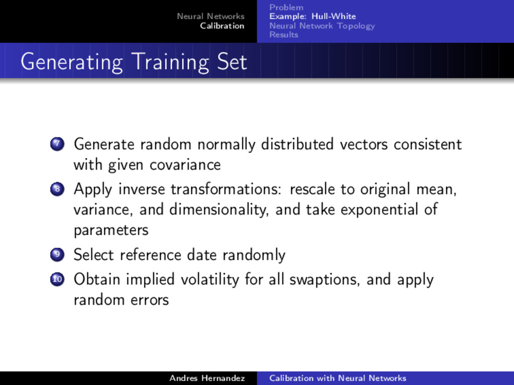
18. Neural Networks Calibration Problem Example: Hull-White Neural Network Topology Results Generating Training Set 7 Generate random normally distributed vectors consistent with given covariance 8 Apply inverse transformations: rescale to original mean, variance, and dimensionality, and take exponential of parameters 9 Select reference date randomly 10 Obtain implied volatility for all swaptions, and apply random errors Andres Hernandez Calibration with Neural Networks
19. Neural Networks Calibration Problem Example: Hull-White Neural Network Topology Results Simple FNN The network used was a ’simple’ feed-forward neural network: Input SWO 156x1 IR 44x1 Hidden Layer a1 = elu(W1p + b1) p 200x1 64x200 W1 1 64x1 b1 + 64x1 Hidden Layer (x3) ai = elu(Wi ai−1 + bi ) 64x64 Wi 1 64x1 bi + 64x1 Output Layer a5 = W5a4 + b5 2x64 W5 1 2x1 b5 + 2x1 Andres Hernandez Calibration with Neural Networks
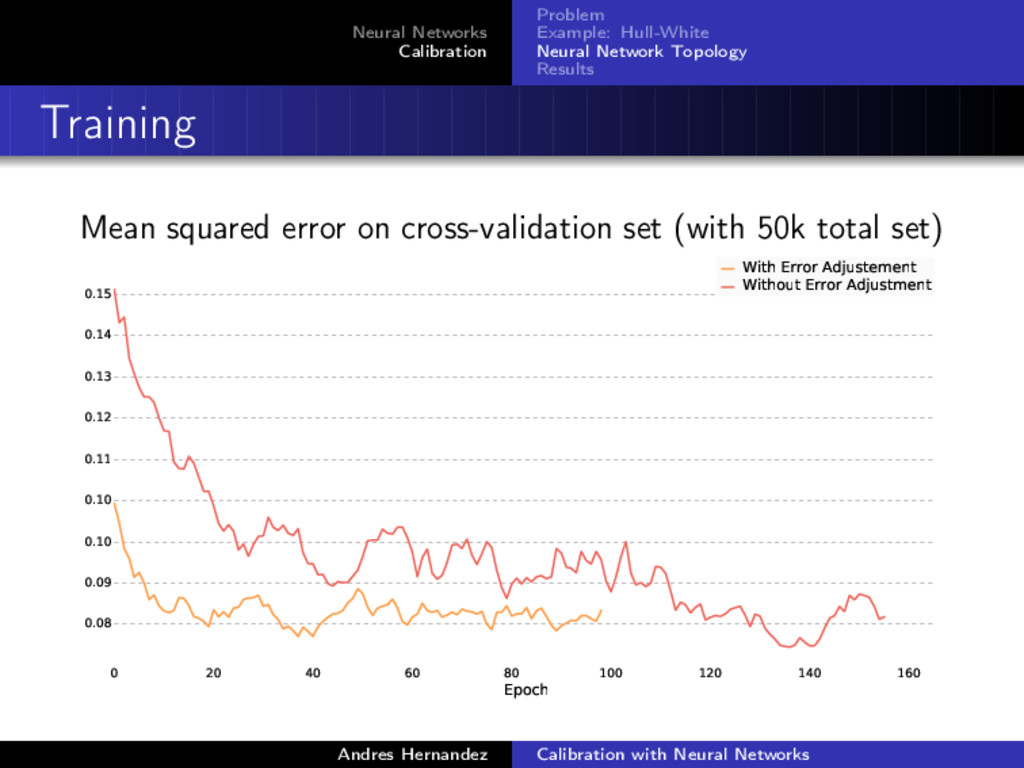
20. Neural Networks Calibration Problem Example: Hull-White Neural Network Topology Results Training Mean squared error on cross-validation set (with 50k total set) 0 20 40 60 80 100 120 140 160 Epoch 0.08 0.09 0.10 0.10 0.11 0.12 0.13 0.14 0.15 With Error Adjustement Without Error Adjustment Andres Hernandez Calibration with Neural Networks
21. Neural Networks Calibration Problem Example: Hull-White Neural Network Topology Results Training Mean squared error on cross-validation set 0 10 20 30 40 50 Epoch 0.068 0.071 0.073 0.075 0.077 0.080 0.082 0.084 0.086 50k_d20 100k_d20 150k_d20 Andres Hernandez Calibration with Neural Networks
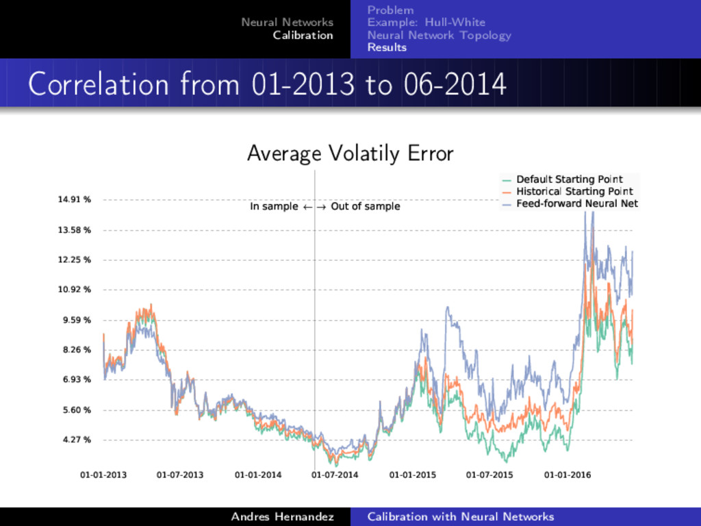
22. Neural Networks Calibration Problem Example: Hull-White Neural Network Topology Results Correlation from 01-2013 to 06-2014 Average Volatily Error 01-01-2013 01-07-2013 01-01-2014 01-07-2014 01-01-2015 01-07-2015 01-01-2016 4.27 % 5.60 % 6.93 % 8.26 % 9.59 % 10.92 % 12.25 % 13.58 % 14.91 % → Out of sample In sample ← Default Starting Point Historical Starting Point Feed-forward Neural Net Andres Hernandez Calibration with Neural Networks
23. Neural Networks Calibration Problem Example: Hull-White Neural Network Topology Results Correlation from 01-2013 to 06-2015 Average Volatily Error 01-01-2013 01-07-2013 01-01-2014 01-07-2014 01-01-2015 01-07-2015 01-01-2016 4.10 % 5.26 % 6.42 % 7.58 % 8.74 % 9.90 % 11.06 % 12.22 % 13.37 % 14.53 % → Out of sample In sample ← Default Starting Point Historical Starting Point Feed-forward Neural Net Andres Hernandez Calibration with Neural Networks
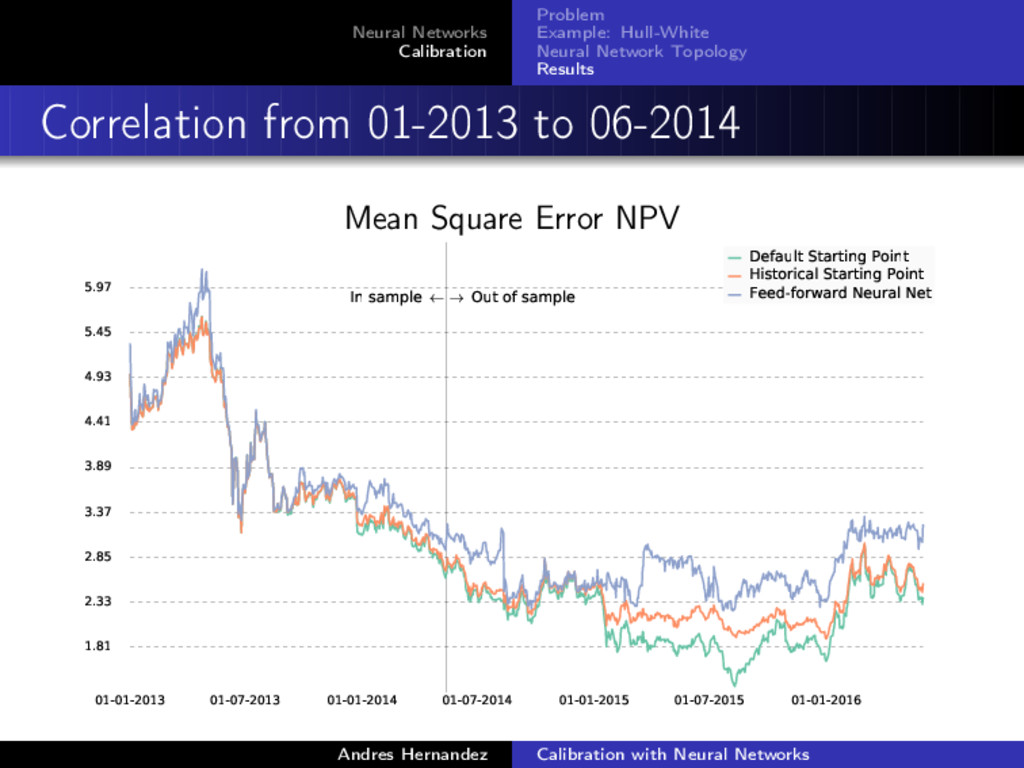
24. Neural Networks Calibration Problem Example: Hull-White Neural Network Topology Results Correlation from 01-2013 to 06-2014 Mean Square Error NPV 01-01-2013 01-07-2013 01-01-2014 01-07-2014 01-01-2015 01-07-2015 01-01-2016 1.81 2.33 2.85 3.37 3.89 4.41 4.93 5.45 5.97 → Out of sample In sample ← Default Starting Point Historical Starting Point Feed-forward Neural Net Andres Hernandez Calibration with Neural Networks
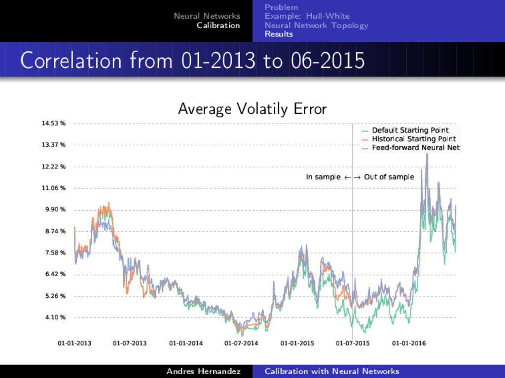
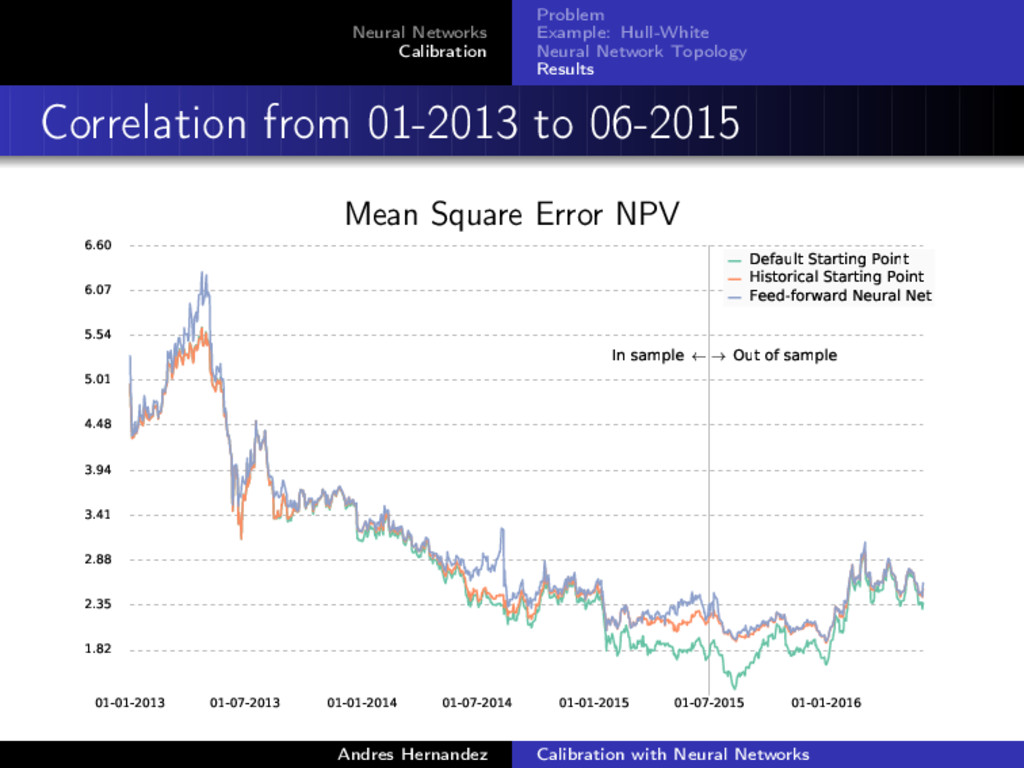
25. Neural Networks Calibration Problem Example: Hull-White Neural Network Topology Results Correlation from 01-2013 to 06-2015 Mean Square Error NPV 01-01-2013 01-07-2013 01-01-2014 01-07-2014 01-01-2015 01-07-2015 01-01-2016 1.82 2.35 2.88 3.41 3.94 4.48 5.01 5.54 6.07 6.60 → Out of sample In sample ← Default Starting Point Historical Starting Point Feed-forward Neural Net Andres Hernandez Calibration with Neural Networks
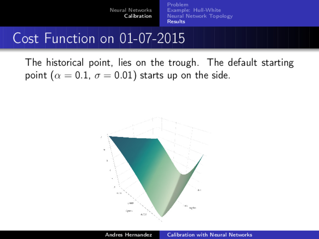
26. Neural Networks Calibration Problem Example: Hull-White Neural Network Topology Results Cost Function on 01-07-2015 The historical point, lies on the trough. The default starting point (α = 0.1, σ = 0.01) starts up on the side. Andres Hernandez Calibration with Neural Networks
27. Neural Networks Calibration Problem Example: Hull-White Neural Network Topology Results FNN Average Volatily Error 01-01-2013 01-07-2013 01-01-2014 01-07-2014 01-01-2015 01-07-2015 01-01-2016 4.47 % 5.99 % 7.52 % 9.04 % 10.57 % 12.10 % 13.62 % 15.15 % 16.67 % → Out of sample In sample ← Default Starting Point FNN Without Error Adjustment FNN With Error Adjustement Andres Hernandez Calibration with Neural Networks
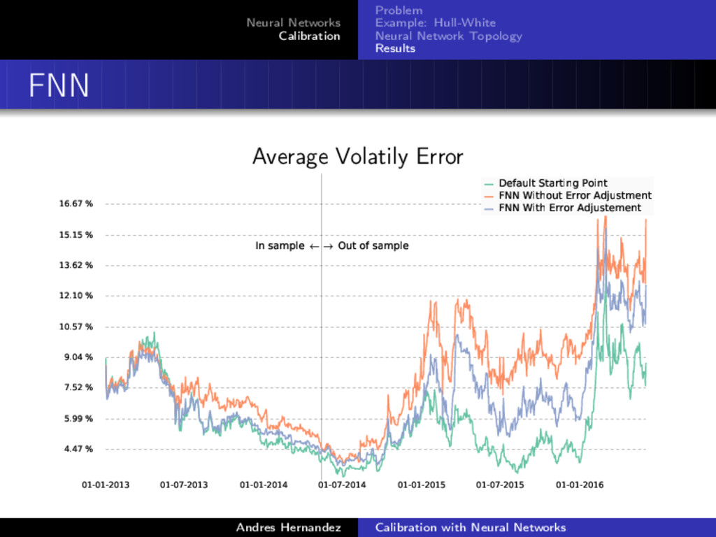
28. Neural Networks Calibration Problem Example: Hull-White Neural Network Topology Results FNN Mean Square Error NPV 01-01-2013 01-07-2013 01-01-2014 01-07-2014 01-01-2015 01-07-2015 01-01-2016 1.82 2.35 2.89 3.42 3.96 4.49 5.02 5.56 6.09 → Out of sample In sample ← Default Starting Point FNN Without Error Adjustment FNN With Error Adjustement Andres Hernandez Calibration with Neural Networks
29. Neural Networks Calibration Problem Example: Hull-White Neural Network Topology Results Further work Sample with parameterized correlation Test with equity volatility models. In particular with large volatility surface and use convolutional neural networks Test with more complex IR models Andres Hernandez Calibration with Neural Networks
30. Neural Networks Calibration Problem Example: Hull-White Neural Network Topology Results Accessing it The example detailed here can be found in my GitHub account: https://github.com/Andres-Hernandez/CalibrationNN To run the code, the following python packages are needed: QuantLib QuantLib Python SWIG bindings Typical python numerical packages: numpy, scipy, pandas, sklearn (, matplotlib) Keras: a deep-learning python library. Requires Theano or TensorFlow as backend Andres Hernandez Calibration with Neural Networks