DataPreparation_SLPrediction

Data Preparation for Sea Level Prediction Studies

Transcript

1. Judith Wells University of Hawaii January 2014 Data Preparation for Sea Level Prediction Studies Discussion Document
2. Hourly tide gauge records from January 1 1979 through December 31 2011. Note that all data are in mm. A: INITIAL DATA
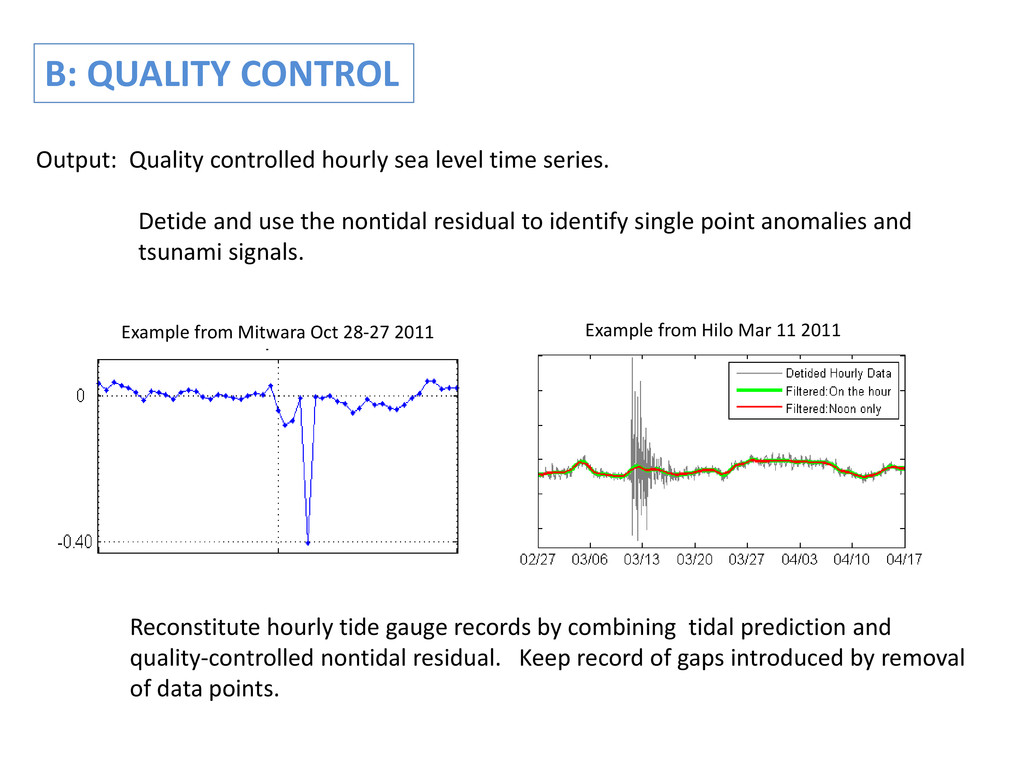
3. Output: Quality controlled hourly sea level time series. Detide and use the nontidal residual to identify single point anomalies and tsunami signals. Reconstitute hourly tide gauge records by combining tidal prediction and quality-controlled nontidal residual. Keep record of gaps introduced by removal of data points. Example from Mitwara Oct 28-27 2011 Example from Hilo Mar 11 2011 B: QUALITY CONTROL
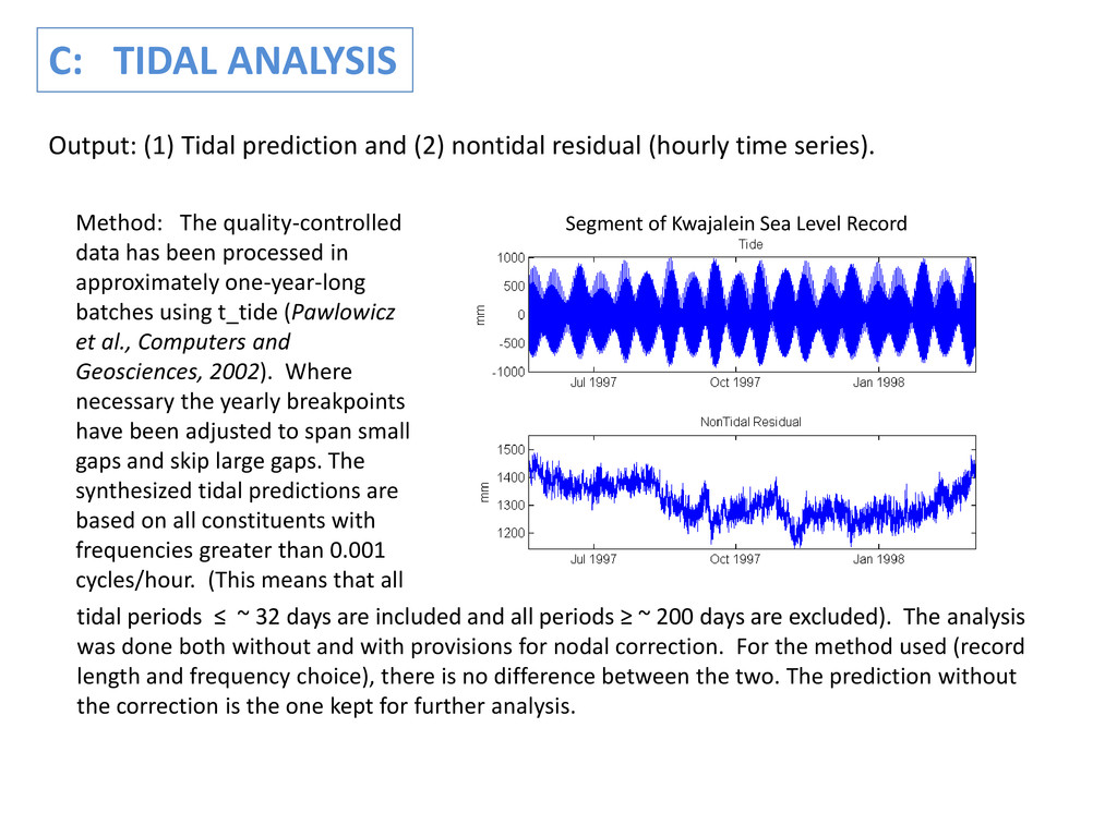
4. Method: The quality-controlled data has been processed in approximately one-year-long batches using t_tide (Pawlowicz et al., Computers and Geosciences, 2002). Where necessary the yearly breakpoints have been adjusted to span small gaps and skip large gaps. The synthesized tidal predictions are based on all constituents with frequencies greater than 0.001 cycles/hour. (This means that all C: TIDAL ANALYSIS Output: (1) Tidal prediction and (2) nontidal residual (hourly time series). Segment of Kwajalein Sea Level Record tidal periods ≤ ~ 32 days are included and all periods ≥ ~ 200 days are excluded). The analysis was done both without and with provisions for nodal correction. For the method used (record length and frequency choice), there is no difference between the two. The prediction without the correction is the one kept for further analysis.
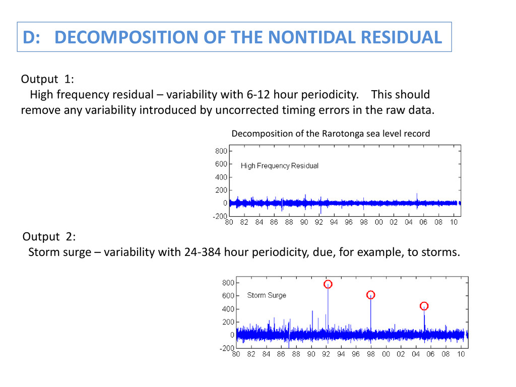
5. Output 1: High frequency residual – variability with 6-12 hour periodicity. This should remove any variability introduced by uncorrected timing errors in the raw data. D: DECOMPOSITION OF THE NONTIDAL RESIDUAL Output 2: Storm surge – variability with 24-384 hour periodicity, due, for example, to storms. Decomposition of the Rarotonga sea level record
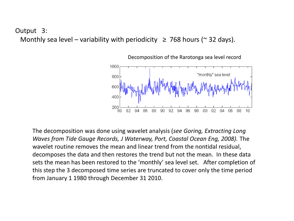
6. The decomposition was done using wavelet analysis (see Goring, Extracting Long Waves from Tide Gauge Records, J Waterway, Port, Coastal Ocean Eng, 2008). The wavelet routine removes the mean and linear trend from the nontidal residual, decomposes the data and then restores the trend but not the mean. In these data sets the mean has been restored to the ‘monthly’ sea level set. After completion of this step the 3 decomposed time series are truncated to cover only the time period from January 1 1980 through December 31 2010. Output 3: Monthly sea level – variability with periodicity ≥ 768 hours (~ 32 days). Decomposition of the Rarotonga sea level record
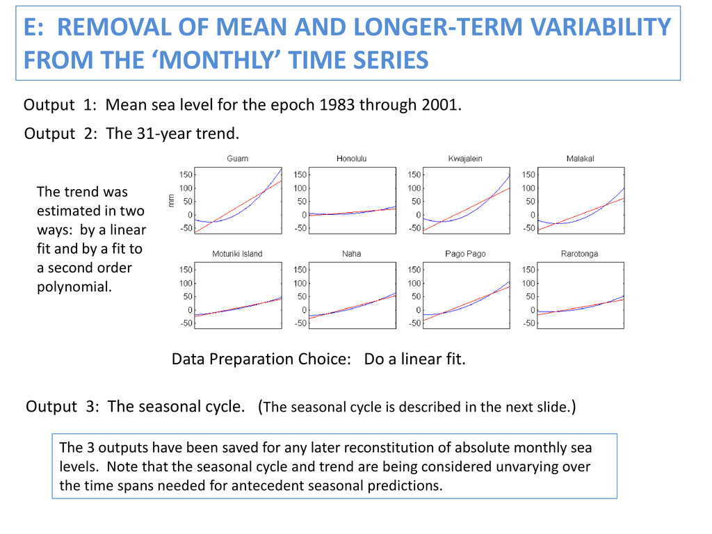
7. E: REMOVAL OF MEAN AND LONGER-TERM VARIABILITY FROM THE ‘MONTHLY’ TIME SERIES Output 1: Mean sea level for the epoch 1983 through 2001. Output 2: The 31-year trend. The trend was estimated in two ways: by a linear fit and by a fit to a second order polynomial. Data Preparation Choice: Do a linear fit. Output 3: The seasonal cycle. (The seasonal cycle is described in the next slide.) The 3 outputs have been saved for any later reconstitution of absolute monthly sea levels. Note that the seasonal cycle and trend are being considered unvarying over the time spans needed for antecedent seasonal predictions.
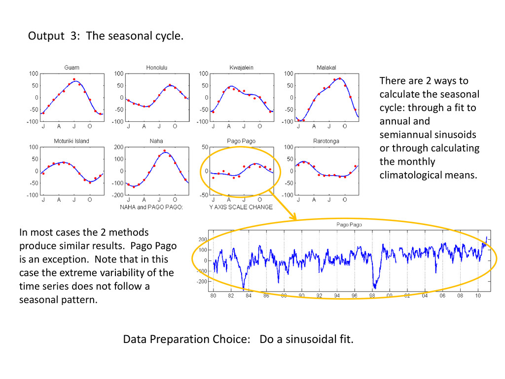
8. Output 3: The seasonal cycle. There are 2 ways to calculate the seasonal cycle: through a fit to annual and semiannual sinusoids or through calculating the monthly climatological means. In most cases the 2 methods produce similar results. Pago Pago is an exception. Note that in this case the extreme variability of the time series does not follow a seasonal pattern. Data Preparation Choice: Do a sinusoidal fit.
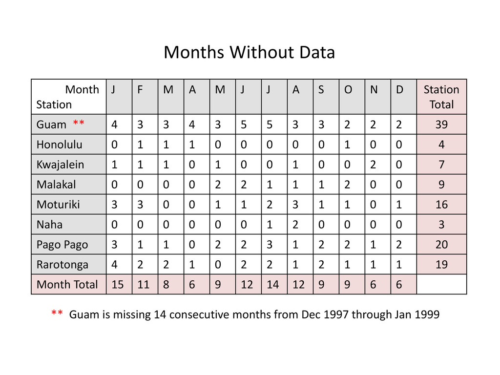
9. • All monthly values have been calculated according to the Level One standards, i.e. the (hourly) data set used for the monthly mean is at least 80% complete with no more than 5 missing days (and no more than 3 missing in a row). Wherever the data failed Level One, it failed Level Two as well and a gap has been left in the monthly record. • Seasonal values are a mean of hourly values over a 3-month period: e.g. JFM or ASO. • Criteria for determining a seasonal value: Either all 3 months meet the Level One criteria for monthly values, or 2 months meet the Level One criteria and hourly data set for the 3rd month is at least 50% complete. F: CALCULATE MONTHLY AND SEASONAL (3-mo) MEANS The monthly and seasonal means are calculated from the demeaned, deseasoned, detrended, “monthly” data. Output 1: Monthly Means Output 2: Seasonal Means
10. Month Station J F M A M J J A S O N D Station Total Guam ** 4 3 3 4 3 5 5 3 3 2 2 2 39 Honolulu 0 1 1 1 0 0 0 0 0 1 0 0 4 Kwajalein 1 1 1 0 1 0 0 1 0 0 2 0 7 Malakal 0 0 0 0 2 2 1 1 1 2 0 0 9 Moturiki 3 3 0 0 1 1 2 3 1 1 0 1 16 Naha 0 0 0 0 0 0 1 2 0 0 0 0 3 Pago Pago 3 1 1 0 2 2 3 1 2 2 1 2 20 Rarotonga 4 2 2 1 0 2 2 1 2 1 1 1 19 Month Total 15 11 8 6 9 12 14 12 9 9 6 6 Months Without Data ** Guam is missing 14 consecutive months from Dec 1997 through Jan 1999
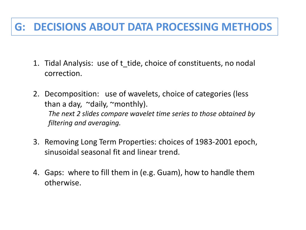
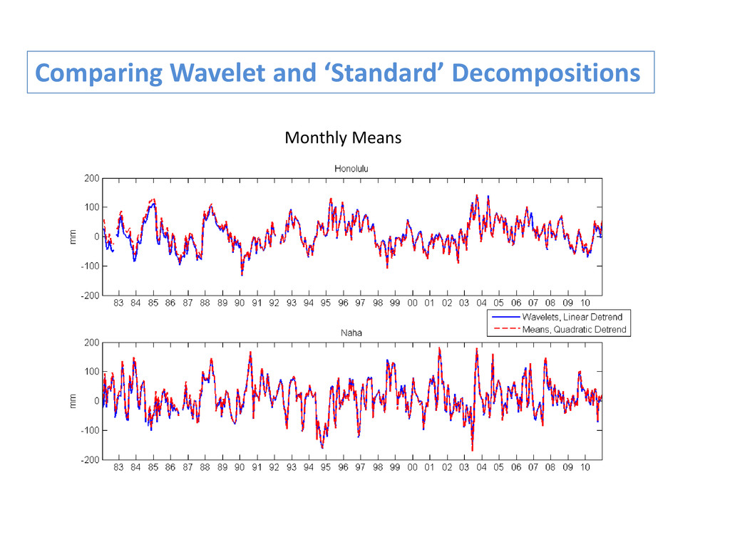
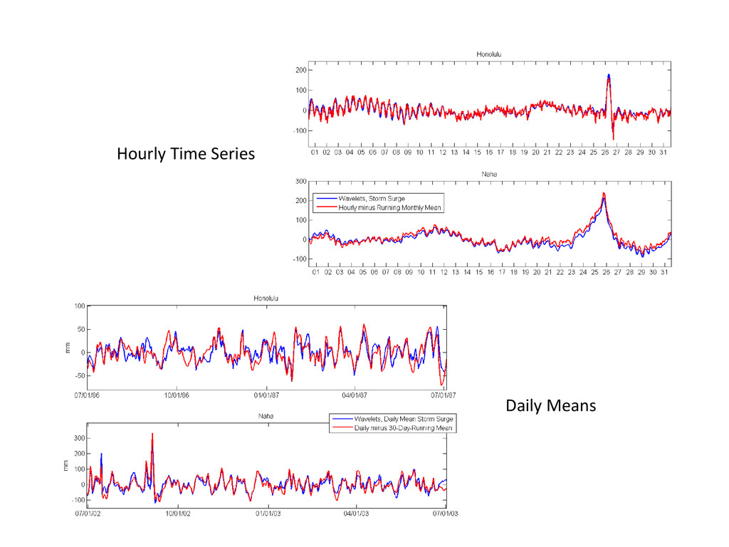
11. G: DECISIONS ABOUT DATA PROCESSING METHODS 1. Tidal Analysis: use of t_tide, choice of constituents, no nodal correction. 2. Decomposition: use of wavelets, choice of categories (less than a day, ~daily, ~monthly). The next 2 slides compare wavelet time series to those obtained by filtering and averaging. 3. Removing Long Term Properties: choices of 1983-2001 epoch, sinusoidal seasonal fit and linear trend. 4. Gaps: where to fill them in (e.g. Guam), how to handle them otherwise.
12. Comparing Wavelet and ‘Standard’ Decompositions Monthly Means
13. Hourly Time Series Daily Means