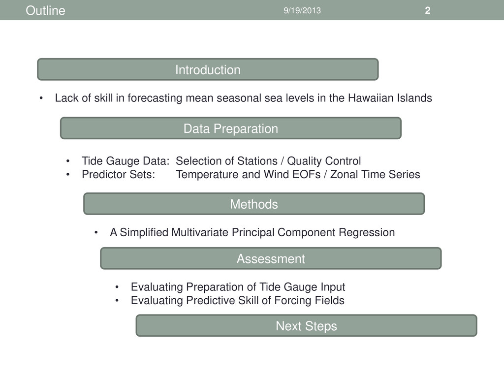
• Lack of skill in forecasting mean seasonal sea levels in the Hawaiian Islands • Tide Gauge Data: Selection of Stations / Quality Control • Predictor Sets: Temperature and Wind EOFs / Zonal Time Series • A Simplified Multivariate Principal Component Regression • Evaluating Preparation of Tide Gauge Input • Evaluating Predictive Skill of Forcing Fields
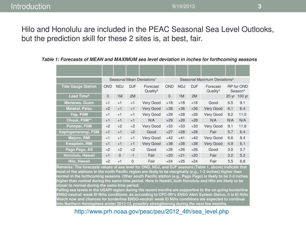
Station OND NDJ DJF Forecast Quality3 OND NDJ DJF Forecast Quality3 RP for OND Season4 Lead Time5 0 1M 2M 0 1M 2M 20 yr 100 yr Marianas, Guam +1 +1 +1 Very Good +18 +18 +18 Good 6.5 9.1 Malakal, Palau +2 +1 +1 Very Good +38 +36 +36 Very Good 6.1 6.4 Yap, FSM +1 +1 +1 Very Good +29 +28 +28 Very Good 8.2 11.0 Chuuk, FSM** +1 +1 +1 N/A +29 +28 +28 N/A N/A N/A Pohnpei, FSM +2 +2 +2 Very Good +33 +33 +33 Very Good 9.1 11.8 Kapingamarangi, FSM +1 +1 +2 Good +27 +28 +28 Fair 5.7 6.4 Majuro, RMI +1 +1 +1 Very Good +42 +41 +42 Very Good 6.6 8.4 Kwajalein, RMI +1 +1 +1 Very Good +38 +38 +38 Very Good 4.9 6.1 Pago Pago, AS +2 +2 +2 Good +26 +26 +26 Good 3.0 3.7 Honolulu, Hawaii +1 0 -1 Fair +20 +21 +20 Fair 3.2 5.2 Hilo, Hawaii +2 +1 0 Fair +24 +25 +24 Fair 5.5 6.8 Remarks: The forecasts values of sea level for OND, NDJ, and DJF seasons (Table 1, above) indicate that most of the stations in the north Pacific region are likely to be marginally (e.g., 1-2 inches) higher than normal in the forthcoming seasons. Other south Pacific station (e.g., Pago Pago) is likely to be 2-3 inches higher than normal during the same time period. Here in Hawaii, both Honolulu and Hilo are likely to be closer to normal during the same time period. Falling sea levels in the USAPI region during the recent months are supportive to the on-going borderline ENSO-neutral/ weak El Niño conditions, as according to CPC-IRI’s ENSO Alert System Status, it is El Niño Watch now and chances for borderline ENSO-neutral/ weak El Niño conditions are expected to continue into Northern Hemisphere winter 2012-13, possibly strengthening during the next few months. Table 1: Forecasts of MEAN and MAXIMUM sea level deviation in inches for forthcoming seasons Introduction http://www.prh.noaa.gov/peac/peu/2012_4th/sea_level.php Hilo and Honolulu are included in the PEAC Seasonal Sea Level Outlooks, but the prediction skill for these 2 sites is, at best, fair.
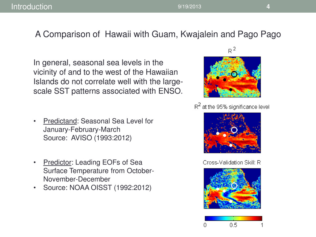
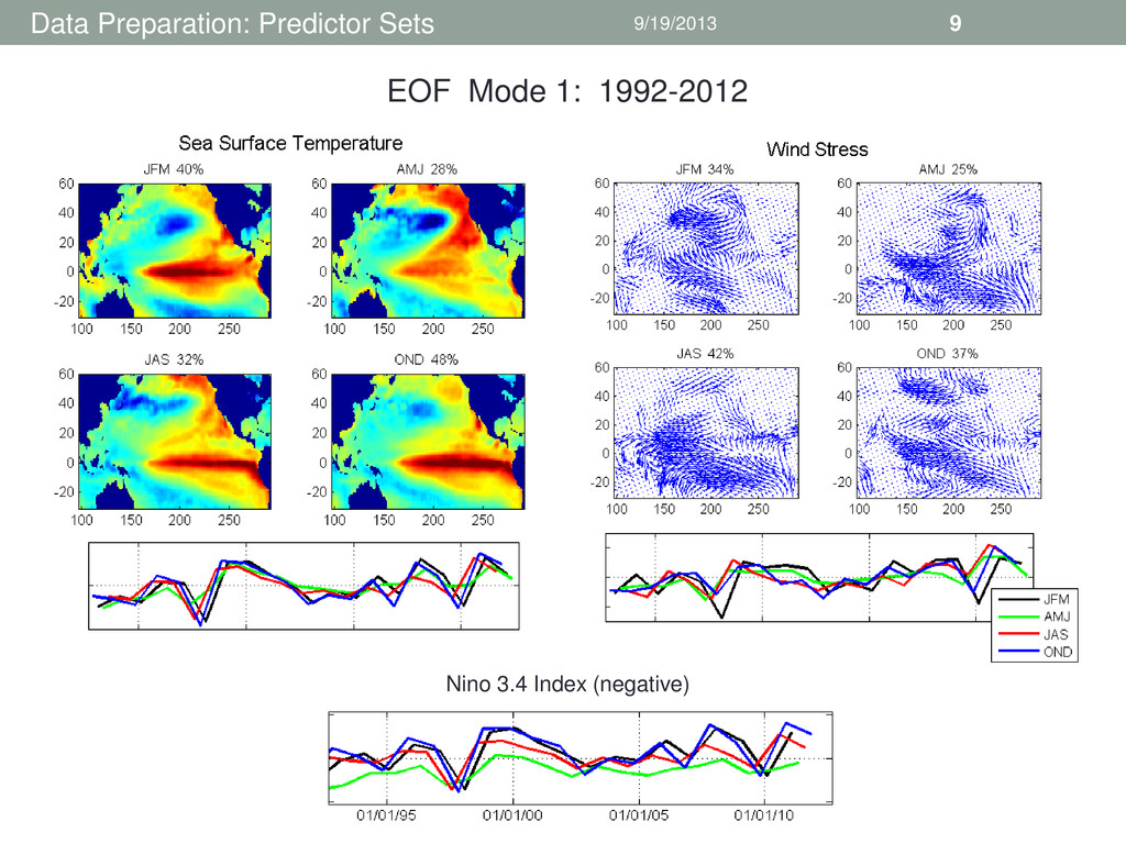
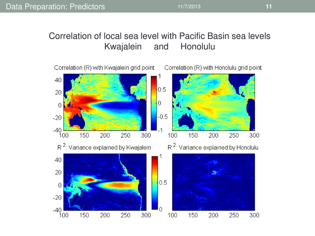
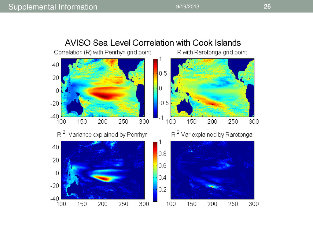
Source: AVISO (1993:2012) • Predictor: Leading EOFs of Sea Surface Temperature from October- November-December • Source: NOAA OISST (1992:2012) In general, seasonal sea levels in the vicinity of and to the west of the Hawaiian Islands do not correlate well with the large- scale SST patterns associated with ENSO. A Comparison of Hawaii with Guam, Kwajalein and Pago Pago
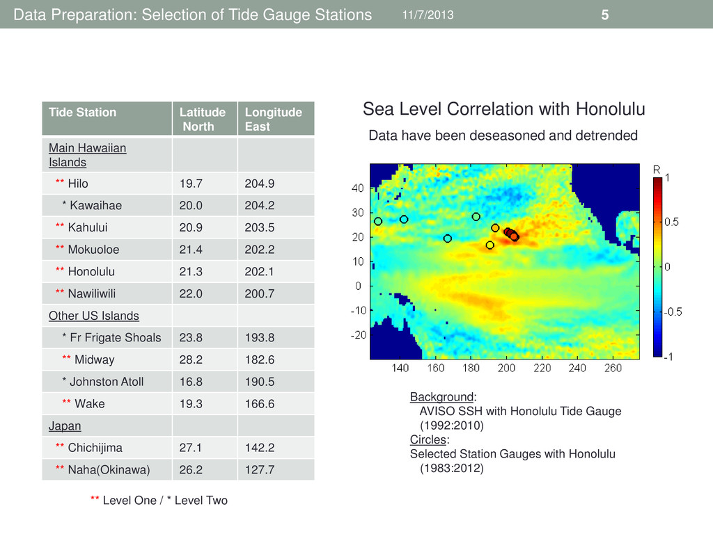
Station Latitude North Longitude East Main Hawaiian Islands ** Hilo 19.7 204.9 * Kawaihae 20.0 204.2 ** Kahului 20.9 203.5 ** Mokuoloe 21.4 202.2 ** Honolulu 21.3 202.1 ** Nawiliwili 22.0 200.7 Other US Islands * Fr Frigate Shoals 23.8 193.8 ** Midway 28.2 182.6 * Johnston Atoll 16.8 190.5 ** Wake 19.3 166.6 Japan ** Chichijima 27.1 142.2 ** Naha(Okinawa) 26.2 127.7 ** Level One / * Level Two Sea Level Correlation with Honolulu Background: AVISO SSH with Honolulu Tide Gauge (1992:2010) Circles: Selected Station Gauges with Honolulu (1983:2012) Data have been deseasoned and detrended
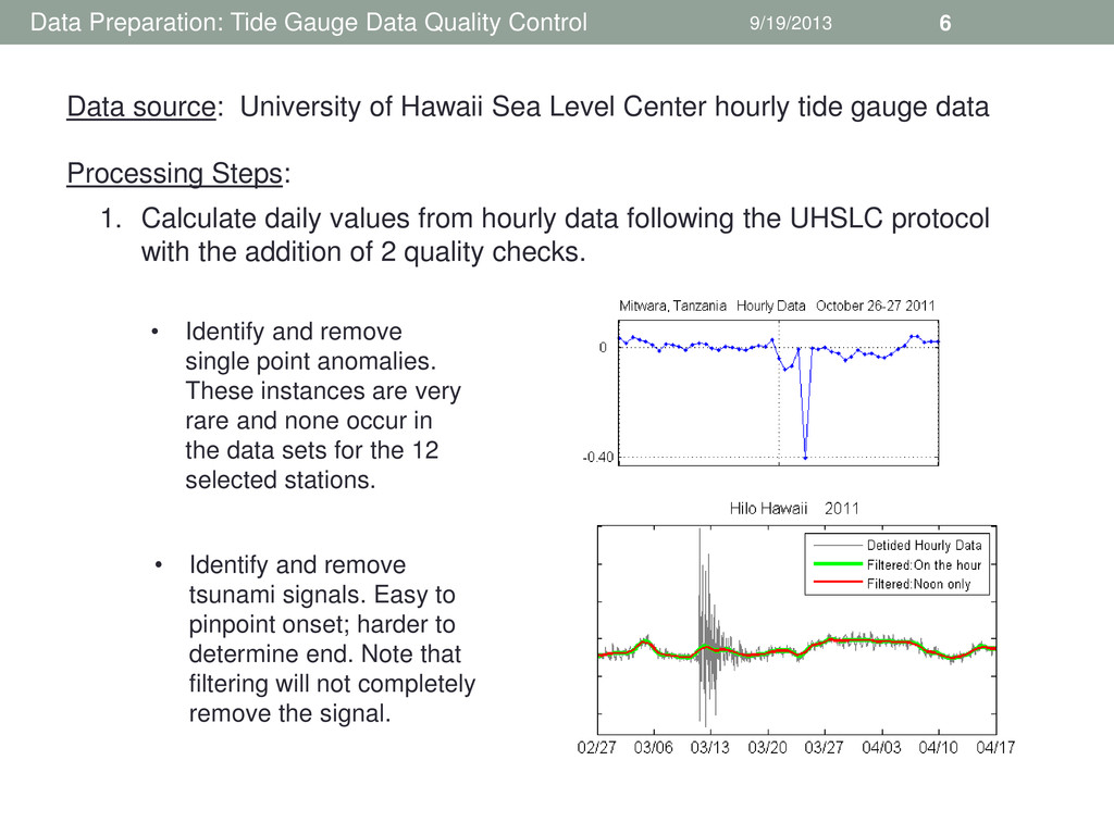
Calculate daily values from hourly data following the UHSLC protocol with the addition of 2 quality checks. Data source: University of Hawaii Sea Level Center hourly tide gauge data Processing Steps: • Identify and remove single point anomalies. These instances are very rare and none occur in the data sets for the 12 selected stations. • Identify and remove tsunami signals. Easy to pinpoint onset; harder to determine end. Note that filtering will not completely remove the signal.
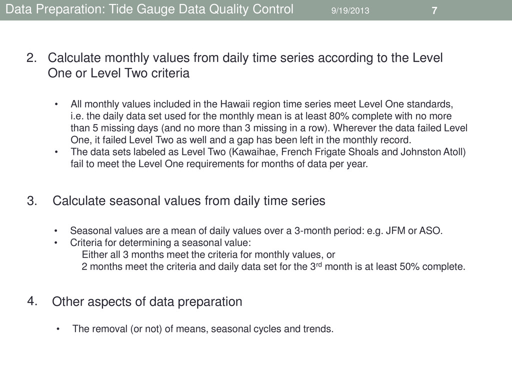
monthly values from daily time series according to the Level One or Level Two criteria 2. • All monthly values included in the Hawaii region time series meet Level One standards, i.e. the daily data set used for the monthly mean is at least 80% complete with no more than 5 missing days (and no more than 3 missing in a row). Wherever the data failed Level One, it failed Level Two as well and a gap has been left in the monthly record. • The data sets labeled as Level Two (Kawaihae, French Frigate Shoals and Johnston Atoll) fail to meet the Level One requirements for months of data per year. Calculate seasonal values from daily time series 3. • Seasonal values are a mean of daily values over a 3-month period: e.g. JFM or ASO. • Criteria for determining a seasonal value: Either all 3 months meet the criteria for monthly values, or 2 months meet the criteria and daily data set for the 3rd month is at least 50% complete. Other aspects of data preparation 4. • The removal (or not) of means, seasonal cycles and trends.
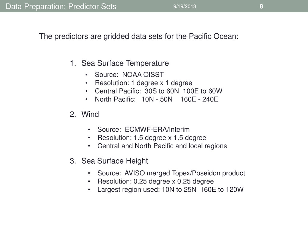
data sets for the Pacific Ocean: 1. Sea Surface Temperature 2. Wind 3. Sea Surface Height • Source: NOAA OISST • Resolution: 1 degree x 1 degree • Central Pacific: 30S to 60N 100E to 60W • North Pacific: 10N - 50N 160E - 240E • Source: ECMWF-ERA/Interim • Resolution: 1.5 degree x 1.5 degree • Central and North Pacific and local regions • Source: AVISO merged Topex/Poseidon product • Resolution: 0.25 degree x 0.25 degree • Largest region used: 10N to 25N 160E to 120W
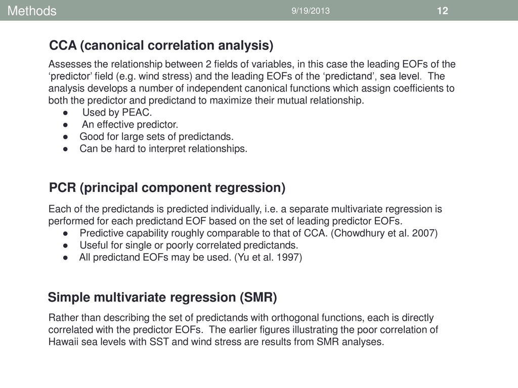
variables, in this case the leading EOFs of the ‘predictor’ field (e.g. wind stress) and the leading EOFs of the ‘predictand’, sea level. The analysis develops a number of independent canonical functions which assign coefficients to both the predictor and predictand to maximize their mutual relationship. • Used by PEAC. • An effective predictor. • Good for large sets of predictands. • Can be hard to interpret relationships. Each of the predictands is predicted individually, i.e. a separate multivariate regression is performed for each predictand EOF based on the set of leading predictor EOFs. • Predictive capability roughly comparable to that of CCA. (Chowdhury et al. 2007) • Useful for single or poorly correlated predictands. • All predictand EOFs may be used. (Yu et al. 1997) Rather than describing the set of predictands with orthogonal functions, each is directly correlated with the predictor EOFs. The earlier figures illustrating the poor correlation of Hawaii sea levels with SST and wind stress are results from SMR analyses. CCA (canonical correlation analysis) PCR (principal component regression) Simple multivariate regression (SMR)
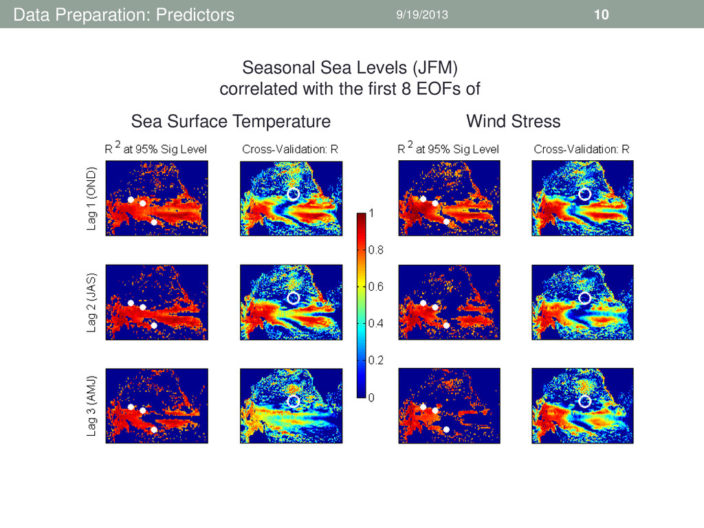
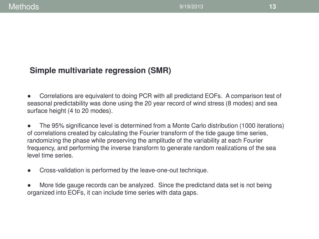
with all predictand EOFs. A comparison test of seasonal predictability was done using the 20 year record of wind stress (8 modes) and sea surface height (4 to 20 modes). • The 95% significance level is determined from a Monte Carlo distribution (1000 iterations) of correlations created by calculating the Fourier transform of the tide gauge time series, randomizing the phase while preserving the amplitude of the variability at each Fourier frequency, and performing the inverse transform to generate random realizations of the sea level time series. • Cross-validation is performed by the leave-one-out technique. • More tide gauge records can be analyzed. Since the predictand data set is not being organized into EOFs, it can include time series with data gaps. Simple multivariate regression (SMR)
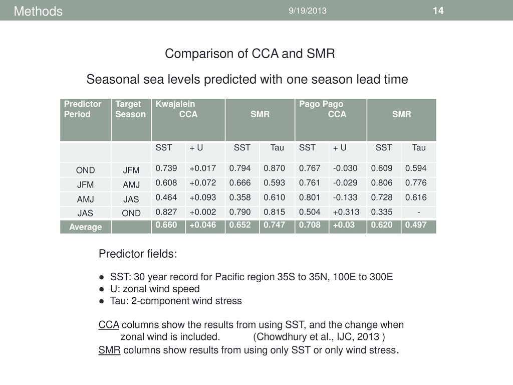
Pago Pago CCA SMR SST + U SST Tau SST + U SST Tau OND JFM 0.739 +0.017 0.794 0.870 0.767 -0.030 0.609 0.594 JFM AMJ 0.608 +0.072 0.666 0.593 0.761 -0.029 0.806 0.776 AMJ JAS 0.464 +0.093 0.358 0.610 0.801 -0.133 0.728 0.616 JAS OND 0.827 +0.002 0.790 0.815 0.504 +0.313 0.335 - Average 0.660 +0.046 0.652 0.747 0.708 +0.03 0.620 0.497 Comparison of CCA and SMR Seasonal sea levels predicted with one season lead time Predictor fields: • SST: 30 year record for Pacific region 35S to 35N, 100E to 300E • U: zonal wind speed • Tau: 2-component wind stress CCA columns show the results from using SST, and the change when zonal wind is included. (Chowdhury et al., IJC, 2013 ) SMR columns show results from using only SST or only wind stress.
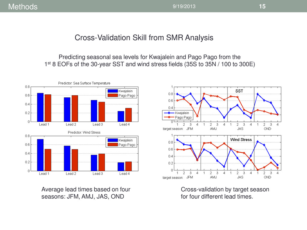
sea levels for Kwajalein and Pago Pago from the 1st 8 EOFs of the 30-year SST and wind stress fields (35S to 35N / 100 to 300E) Average lead times based on four seasons: JFM, AMJ, JAS, OND Cross-validation by target season for four different lead times.
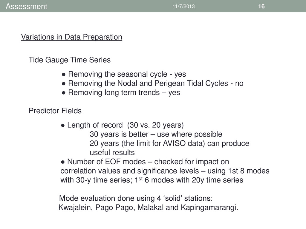
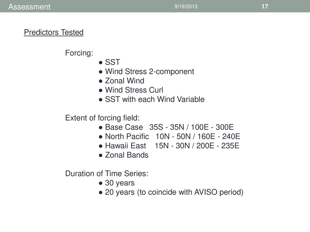
Series • Removing the seasonal cycle - yes • Removing the Nodal and Perigean Tidal Cycles - no • Removing long term trends – yes Predictor Fields • Length of record (30 vs. 20 years) 30 years is better – use where possible 20 years (the limit for AVISO data) can produce useful results • Number of EOF modes – checked for impact on correlation values and significance levels – using 1st 8 modes with 30-y time series; 1st 6 modes with 20y time series Mode evaluation done using 4 ‘solid’ stations: Kwajalein, Pago Pago, Malakal and Kapingamarangi.
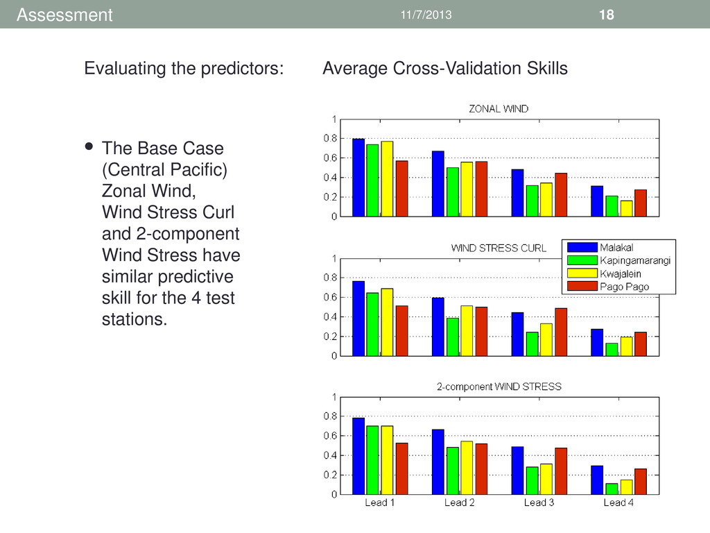
Stress Curl and 2-component Wind Stress have similar predictive skill for the 4 test stations. Evaluating the predictors: Average Cross-Validation Skills • Assessment
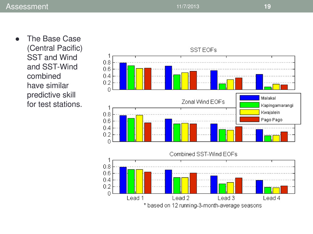
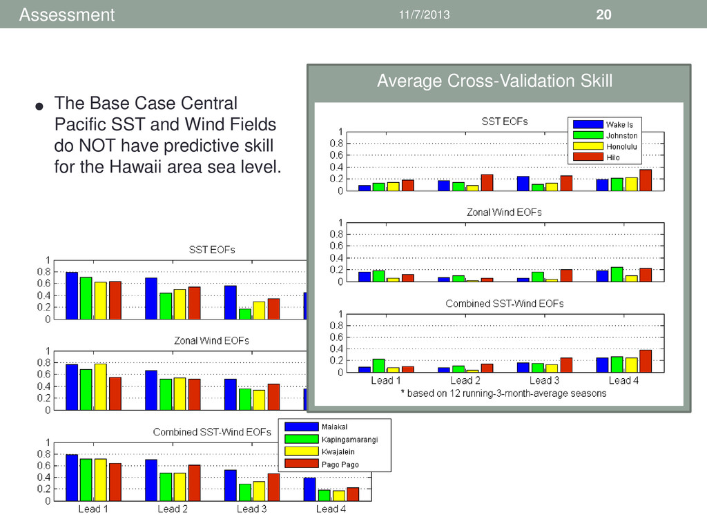
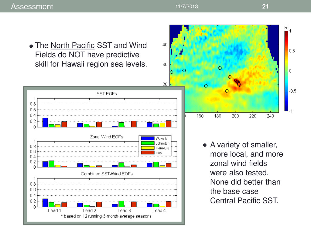
do NOT have predictive skill for Hawaii region sea levels. • A variety of smaller, more local, and more zonal wind fields were also tested. None did better than the base case Central Pacific SST. •
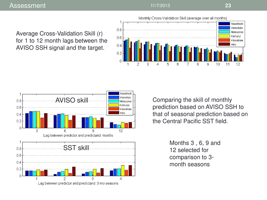
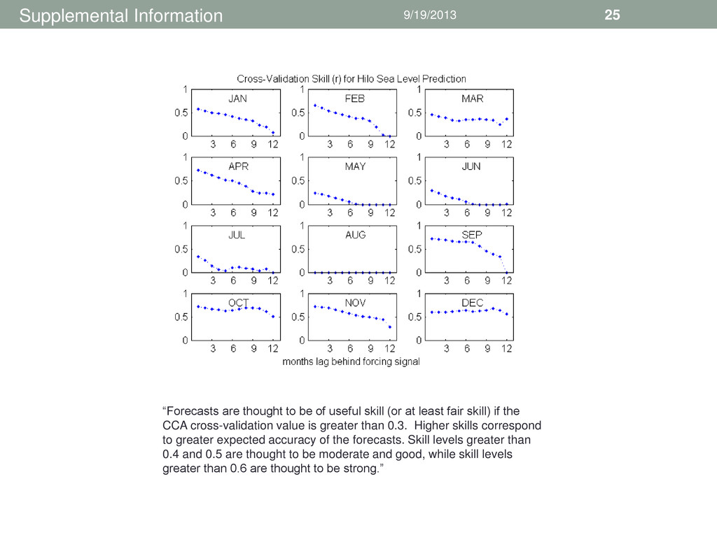
12 month lags between the AVISO SSH signal and the target. Months 3 , 6, 9 and 12 selected for comparison to 3- month seasons Comparing the skill of monthly prediction based on AVISO SSH to that of seasonal prediction based on the Central Pacific SST field. SST skill AVISO skill
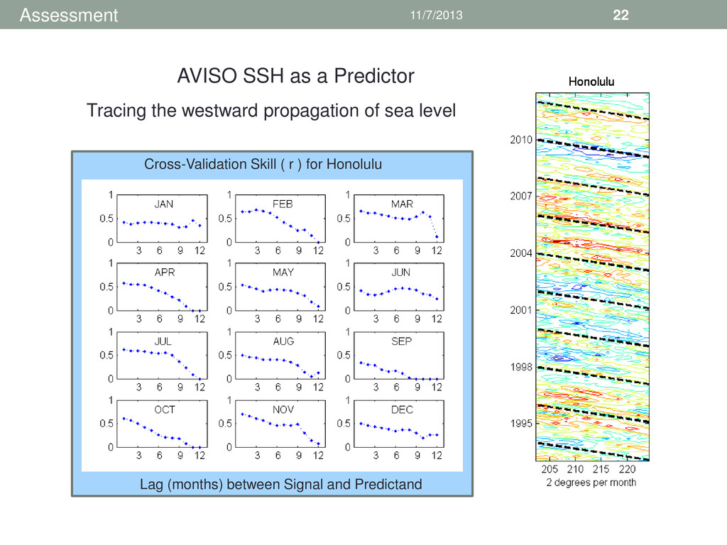
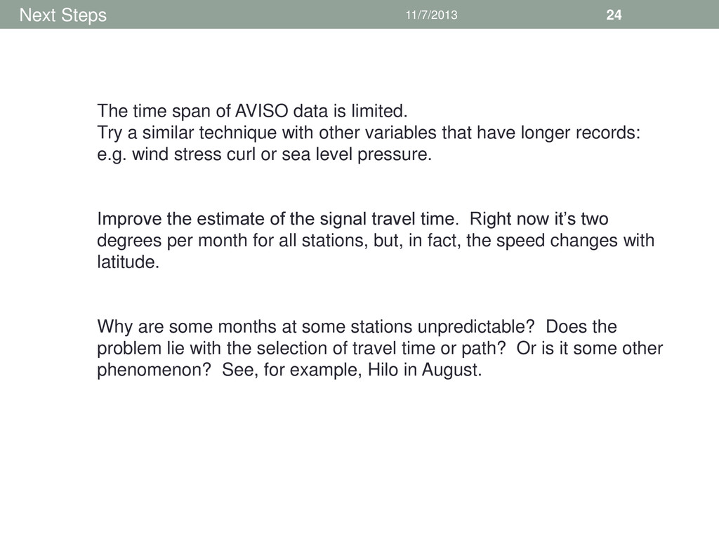
is limited. Try a similar technique with other variables that have longer records: e.g. wind stress curl or sea level pressure. Improve the estimate of the signal travel time. Right now it’s two degrees per month for all stations, but, in fact, the speed changes with latitude. Why are some months at some stations unpredictable? Does the problem lie with the selection of travel time or path? Or is it some other phenomenon? See, for example, Hilo in August.
useful skill (or at least fair skill) if the CCA cross-validation value is greater than 0.3. Higher skills correspond to greater expected accuracy of the forecasts. Skill levels greater than 0.4 and 0.5 are thought to be moderate and good, while skill levels greater than 0.6 are thought to be strong.”


 judithwells
 szymonslowik
 lcolladotor
 katarinadahlin
 moore
 keathley
 inesmontani
 helmedeiros
 eitanlees
 mraible
 paigeccino
 skipperchong
 marcoroth