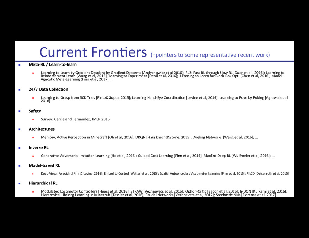
with Q-Learning n DDPG [Lillicrap et al, 2015]; Q-prop [Gu et al, 2016]; Doubly Robust [Dudik et al, 2011]; Deep Energy Q [Haarnoja*, Tang* etal, 2016] n PGQ [O’Donoghue et al, 2016]; ACER [Wang et al, 2016]; Q(lambda) [Harutyunyan et al, 2016]; Retrace(lambda) [Munos et al, 2016], Equivalence PG and SoU-Q [Schulman et al, 2017],… n Explora5on n VIME [HouthooU et al, 2016]; Count-Based ExploraRon [Bellemare et al, 2016]; #ExploraRon [Tang et al, 2016]; Curiosity [Schmidhueber, 1991]; Parameter Space Noise for ExploraRon [Plappert et al, 2017]; Noisy Networks [Fortunato et al, 2017] n Auxiliary objec5ves n Learning to Navigate [Mirowski et al, 2016]; RL with Unsupervised Auxiliary Tasks [Jaderberg et al, 2016], … n Mul5-task and transfer (incl. sim2real) n DeepDriving [Chen et al, 2015]; Progressive Nets [Rusu et al, 2016]; Flight without a Real Image [Sadeghi & Levine, 2016]; Sim2Real Visuomotor [Tzeng et al, 2016]; Sim2Real Inverse Dynamics [ChrisRano et al, 2016]; Modular NNs [Devin*, Gupta*, et al 2016]; Domain RandomizaRon [Tobin et al, 2017] n Language n Learning to Communicate [Foerster et al, 2016]; MulRtask RL w/Policy Sketches [Andreas et al, 2016]; Learning Language through InteracRon [Wang et al, 2016] Current FronRers (+pointers to some representaRve recent work) John Schulman & Pieter Abbeel – OpenAI + UC Berkeley
![Reinforcement Learning [Figure source: SuIon & Barto, 1998] John Schulman](https://files.speakerdeck.com/presentations/d9489d8dde7b4ded9092ff685a5502e4/slide_1.jpg)
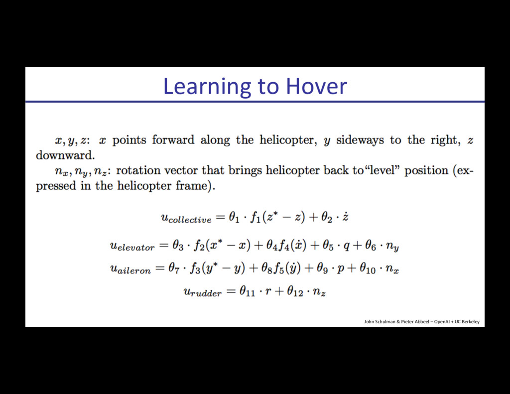
![[Ng + al, ISER 2004] [Policy search was done in](https://files.speakerdeck.com/presentations/d9489d8dde7b4ded9092ff685a5502e4/slide_40.jpg)
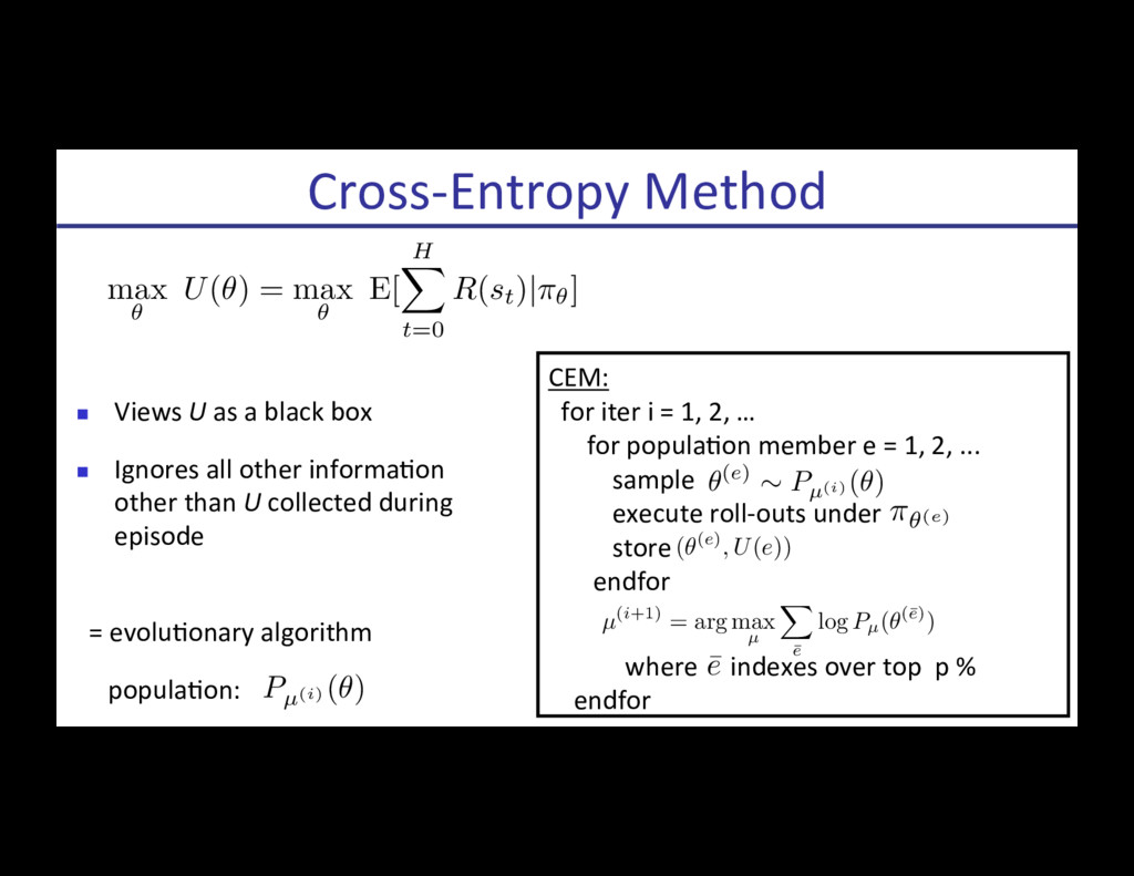
![n Can work embarrassingly well Cross-Entropy Method [NIPS 2013] John](https://files.speakerdeck.com/presentations/d9489d8dde7b4ded9092ff685a5502e4/slide_44.jpg)
![[Salimans, Ho, Chen, Sutskever, 2017] ConsideraRons n Pros: n Work](https://files.speakerdeck.com/presentations/d9489d8dde7b4ded9092ff685a5502e4/slide_48.jpg)
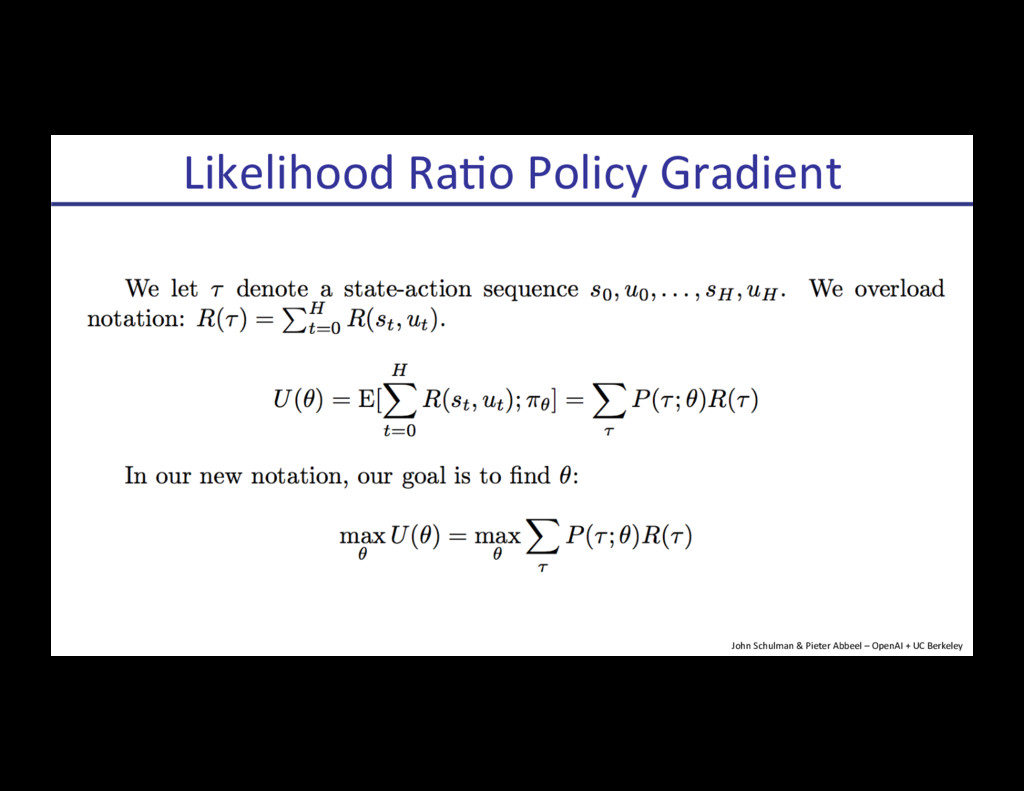
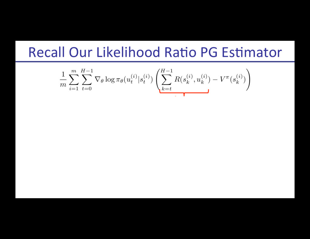
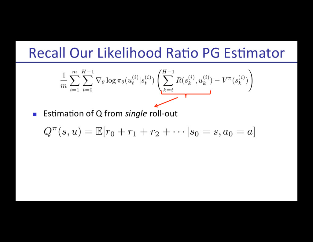
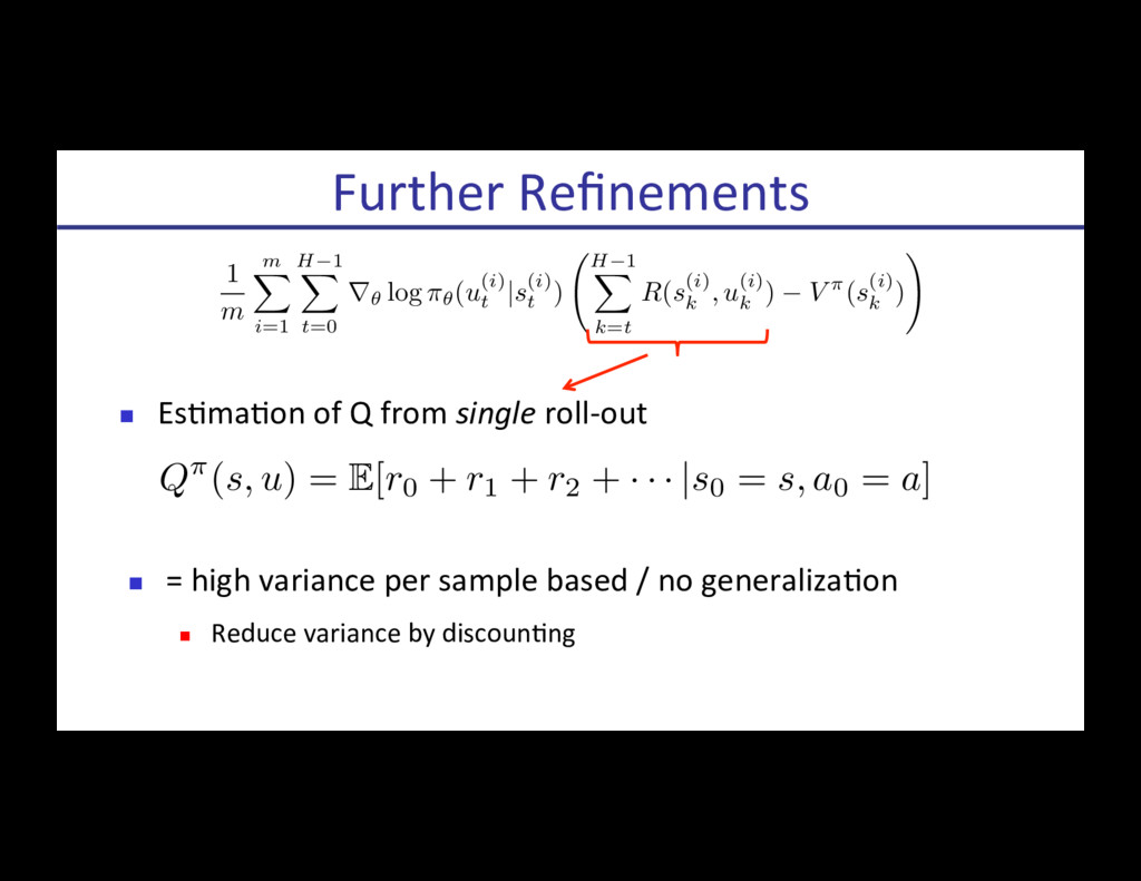
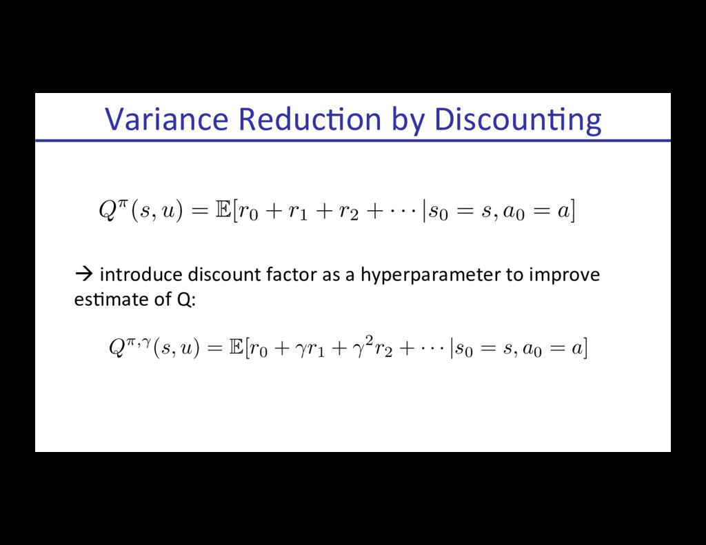
![Likelihood RaRo Policy Gradient [Aleksandrov, Sysoyev, & Shemeneva, 1968] [Rubinstein,](https://files.speakerdeck.com/presentations/d9489d8dde7b4ded9092ff685a5502e4/slide_51.jpg)
![Likelihood RaRo Policy Gradient [Aleksandrov, Sysoyev, & Shemeneva, 1968] [Rubinstein,](https://files.speakerdeck.com/presentations/d9489d8dde7b4ded9092ff685a5502e4/slide_52.jpg)
![Likelihood RaRo Policy Gradient [Aleksandrov, Sysoyev, & Shemeneva, 1968] [Rubinstein,](https://files.speakerdeck.com/presentations/d9489d8dde7b4ded9092ff685a5502e4/slide_53.jpg)
![Likelihood RaRo Policy Gradient [Aleksandrov, Sysoyev, & Shemeneva, 1968] [Rubinstein,](https://files.speakerdeck.com/presentations/d9489d8dde7b4ded9092ff685a5502e4/slide_54.jpg)
![Likelihood RaRo Policy Gradient [Aleksandrov, Sysoyev, & Shemeneva, 1968] [Rubinstein,](https://files.speakerdeck.com/presentations/d9489d8dde7b4ded9092ff685a5502e4/slide_55.jpg)
![Likelihood RaRo Policy Gradient [Aleksandrov, Sysoyev, & Shemeneva, 1968] [Rubinstein,](https://files.speakerdeck.com/presentations/d9489d8dde7b4ded9092ff685a5502e4/slide_56.jpg)
![Pseudo-code Reinforce aka Vanilla Policy Gradient ~ [Williams, 1992] John](https://files.speakerdeck.com/presentations/d9489d8dde7b4ded9092ff685a5502e4/slide_72.jpg)
![[Schulman, Levine, Moritz, Jordan, Abbeel, 2014] Experiments in LocomoRon](https://files.speakerdeck.com/presentations/d9489d8dde7b4ded9092ff685a5502e4/slide_96.jpg)
![n Deep Q-Network (DQN) [Mnih et al, 2013/2015] n Dagger](https://files.speakerdeck.com/presentations/d9489d8dde7b4ded9092ff685a5502e4/slide_99.jpg)
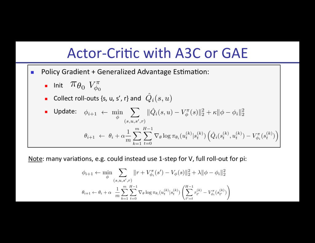
![n Async Advantage Actor Cri-c (A3C) [Mnih et al, 2016]](https://files.speakerdeck.com/presentations/d9489d8dde7b4ded9092ff685a5502e4/slide_113.jpg)
![n Generalized Advantage Es-ma-on (GAE) [Schulman et al, ICLR 2016]](https://files.speakerdeck.com/presentations/d9489d8dde7b4ded9092ff685a5502e4/slide_114.jpg)
![n Generalized Advantage Es-ma-on (GAE) [Schulman et al, ICLR 2016]](https://files.speakerdeck.com/presentations/d9489d8dde7b4ded9092ff685a5502e4/slide_115.jpg)
![n [Mnih et al, ICML 2016] n Likelihood RaRo Policy](https://files.speakerdeck.com/presentations/d9489d8dde7b4ded9092ff685a5502e4/slide_117.jpg)
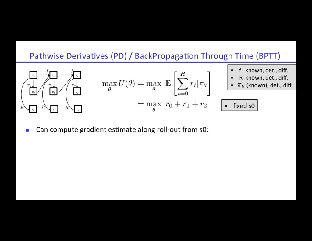
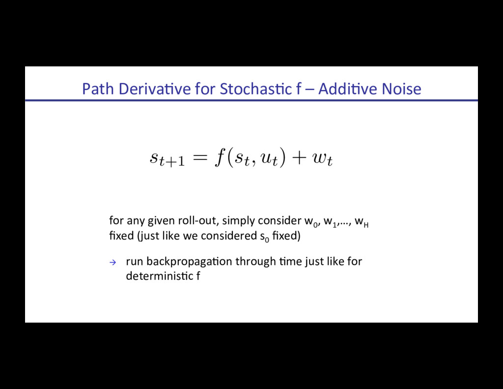
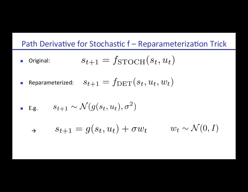
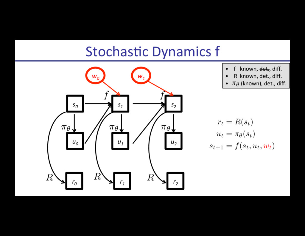
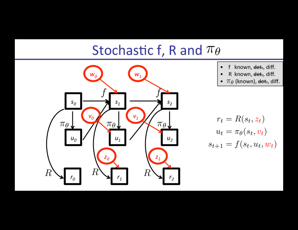
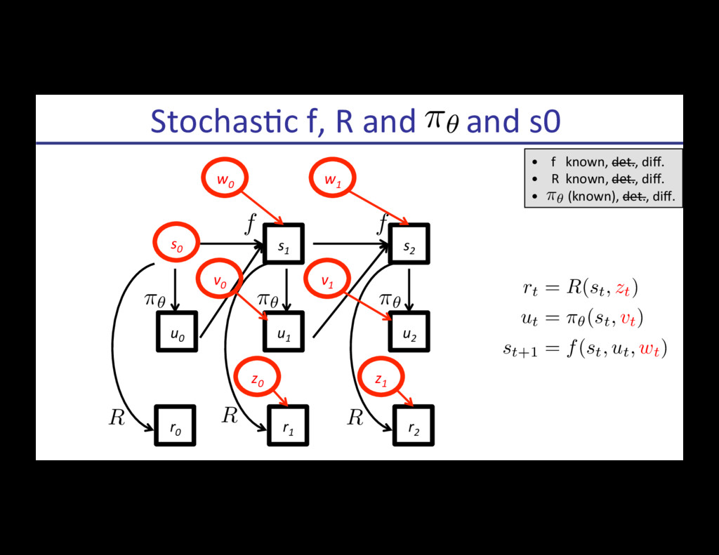
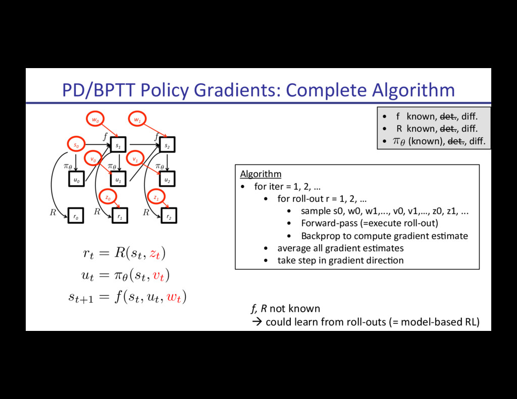
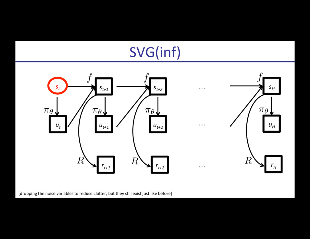
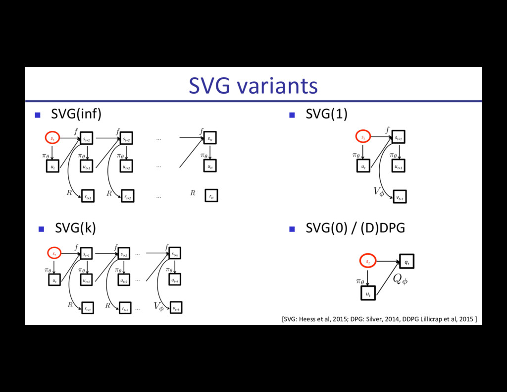
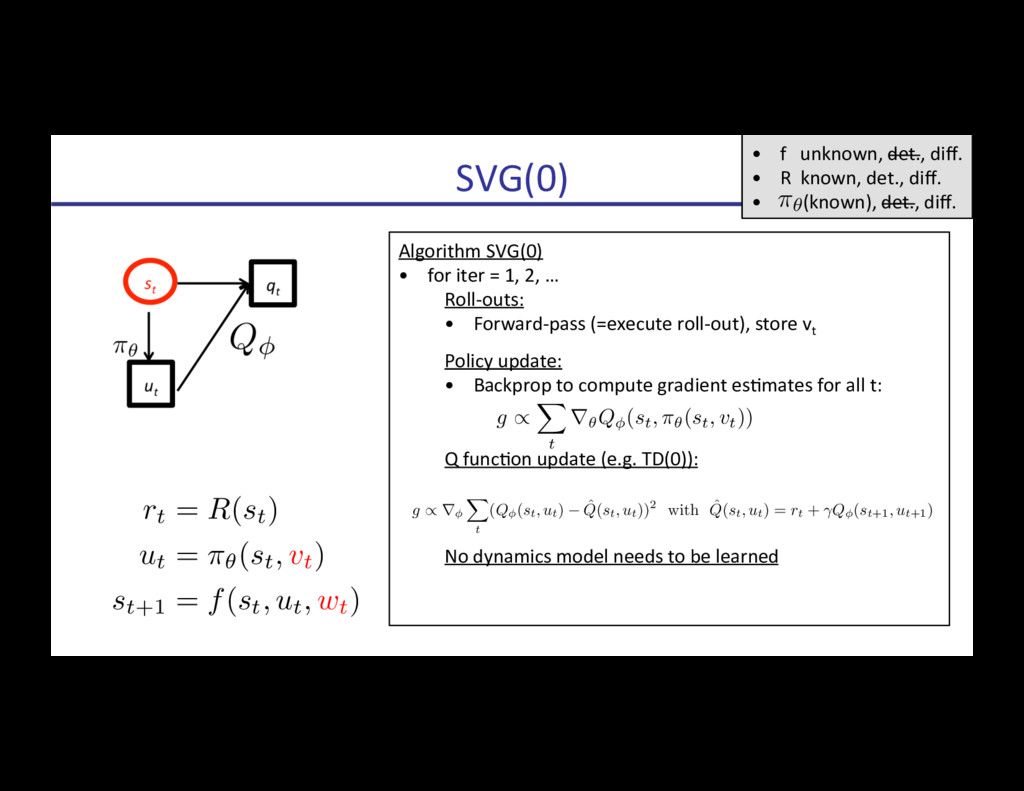
![[Schulman, Heess, Weber, Abbeel, NIPS 2015] StochasRc ComputaRon Graphs](https://files.speakerdeck.com/presentations/d9489d8dde7b4ded9092ff685a5502e4/slide_122.jpg)
![[Schulman, Heess, Weber, Abbeel, NIPS 2015] StochasRc ComputaRon Graphs](https://files.speakerdeck.com/presentations/d9489d8dde7b4ded9092ff685a5502e4/slide_123.jpg)
![[Schulman, Heess, Weber, Abbeel, NIPS 2015] StochasRc ComputaRon Graphs](https://files.speakerdeck.com/presentations/d9489d8dde7b4ded9092ff685a5502e4/slide_124.jpg)
![[Schulman, Heess, Weber, Abbeel, NIPS 2015] StochasRc ComputaRon Graphs](https://files.speakerdeck.com/presentations/d9489d8dde7b4ded9092ff685a5502e4/slide_125.jpg)
![[Schulman, Heess, Weber, Abbeel, NIPS 2015] StochasRc ComputaRon Graphs](https://files.speakerdeck.com/presentations/d9489d8dde7b4ded9092ff685a5502e4/slide_126.jpg)
![[Schulman, Heess, Weber, Abbeel, NIPS 2015] StochasRc ComputaRon Graphs](https://files.speakerdeck.com/presentations/d9489d8dde7b4ded9092ff685a5502e4/slide_127.jpg)
![[Schulman, Heess, Weber, Abbeel, NIPS 2015] StochasRc ComputaRon Graphs](https://files.speakerdeck.com/presentations/d9489d8dde7b4ded9092ff685a5502e4/slide_128.jpg)
![[Schulman, Heess, Weber, Abbeel, NIPS 2015] StochasRc ComputaRon Graphs](https://files.speakerdeck.com/presentations/d9489d8dde7b4ded9092ff685a5502e4/slide_129.jpg)
![[Schulman, Heess, Weber, Abbeel, NIPS 2015] StochasRc ComputaRon Graphs](https://files.speakerdeck.com/presentations/d9489d8dde7b4ded9092ff685a5502e4/slide_130.jpg)
![[Schulman, Heess, Weber, Abbeel, NIPS 2015] StochasRc ComputaRon Graphs](https://files.speakerdeck.com/presentations/d9489d8dde7b4ded9092ff685a5502e4/slide_131.jpg)