Lec10.2.MultipleRegression.pdf

Transcript

1. Multiple Regression Matthew J. Salganik POL 345/SOC 305 Introduction to Quantitative Social Science Princeton University Wednesday, November 29, 2017
2. Your future courses Omar Wasow from POL 346 Applied Quantitative Analysis
3. Your future courses
4. Logistics QSS assignments due 24 hours before precept
5. Logistics QSS assignments due 24 hours before precept Pset 3 will be posted W 12/6 and due W 12/13
6. Logistics QSS assignments due 24 hours before precept Pset 3 will be posted W 12/6 and due W 12/13 COMPASS workshop: Thurs, 11/30 Text Mining in R (Ethan)
7. Goals for today See real data analyis workflow (with data wrangling)
8. Goals for today See real data analyis workflow (with data wrangling) Review difference-of-means
9. Goals for today See real data analyis workflow (with data wrangling) Review difference-of-means Show connection between difference-of-means and regression
10. Goals for today See real data analyis workflow (with data wrangling) Review difference-of-means Show connection between difference-of-means and regression Explore multiple regression with continuous and dummy variables in equations, code, pictures, and words
11. Goals for today See real data analyis workflow (with data wrangling) Review difference-of-means Show connection between difference-of-means and regression Explore multiple regression with continuous and dummy variables in equations, code, pictures, and words Learn something about Twitter
12. https://www.theatlantic.com/technology/archive/2017/10/ twitters-harassment-problem-is-baked-into-its-design/542952/
13. http://dx.doi.org/10.1007/s11109-016-9373-5
14. https://github.com/kmunger/ Replication-Materials-for-Tweetment-Effects-on-the-Tweeted
15. See paper for more on the sampling procedure
18. 2 x 2 design
19. Why do we need an experiment?
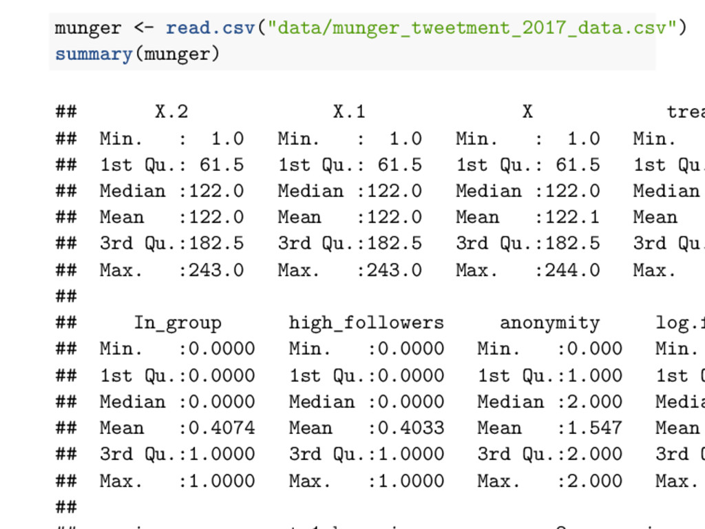
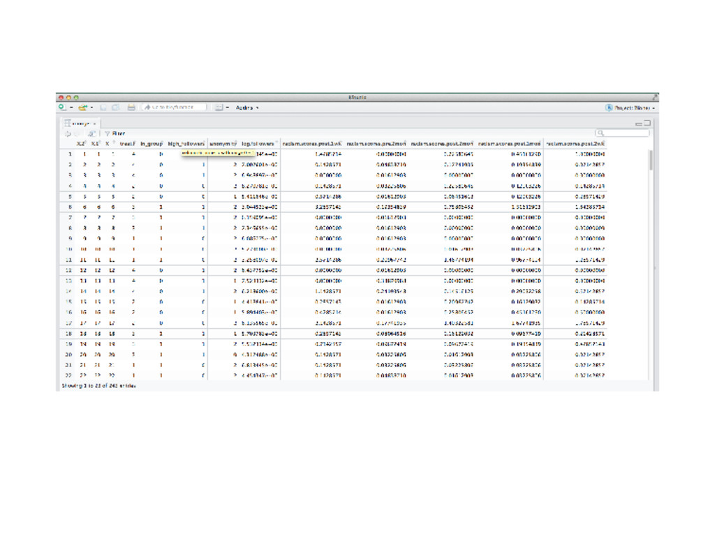
20. munger <- read.csv("data/munger_tweetment_2017_data.csv") summary(munger) ## X.2 X.1 X trea ## Min. : 1.0 Min. : 1.0 Min. : 1.0 Min. ## 1st Qu.: 61.5 1st Qu.: 61.5 1st Qu.: 61.5 1st Qu. ## Median :122.0 Median :122.0 Median :122.0 Median ## Mean :122.0 Mean :122.0 Mean :122.1 Mean ## 3rd Qu.:182.5 3rd Qu.:182.5 3rd Qu.:182.5 3rd Qu. ## Max. :243.0 Max. :243.0 Max. :244.0 Max. ## ## In_group high_followers anonymity log.f ## Min. :0.0000 Min. :0.0000 Min. :0.000 Min. ## 1st Qu.:0.0000 1st Qu.:0.0000 1st Qu.:1.000 1st Q ## Median :0.0000 Median :0.0000 Median :2.000 Media ## Mean :0.4074 Mean :0.4033 Mean :1.547 Mean ## 3rd Qu.:1.0000 3rd Qu.:1.0000 3rd Qu.:2.000 3rd Q ## Max. :1.0000 Max. :1.0000 Max. :2.000 Max. ##
22. Data wrangling barplot(table(munger$treat.f)) 0 1 2 3 4 0 10 20 30 40 50
23. Data wrangling str(munger$treat.f) ## int [1:243] 4 4 4 2 2 3 3 3 1 1 ...
24. Data wrangling
25. Data wrangling
26. Data wrangling munger$treat.f <- as.factor(munger$treat.f) # 0 = control # 1 = in-group, low followers # 2 = out-group, low followers # 3 = in-group, high followers # 4 = out-group, high followers levels(munger$treat.f) <- c("control", "in-group/low", "out-group/low", "in-group/high", "out-group/high")
27. Data wrangling barplot(table(munger$treat.f)) control in−group/low out−group/low in−group/high out−group/high 0 10 20 30 40 50
28. Data wrangling Why am I not adding more informative labels?
29. Data wrangling Histogram of munger$racism.scores.post.1wk munger$racism.scores.post.1wk Frequency 0 1 2 3 4 5 0 50 100 150
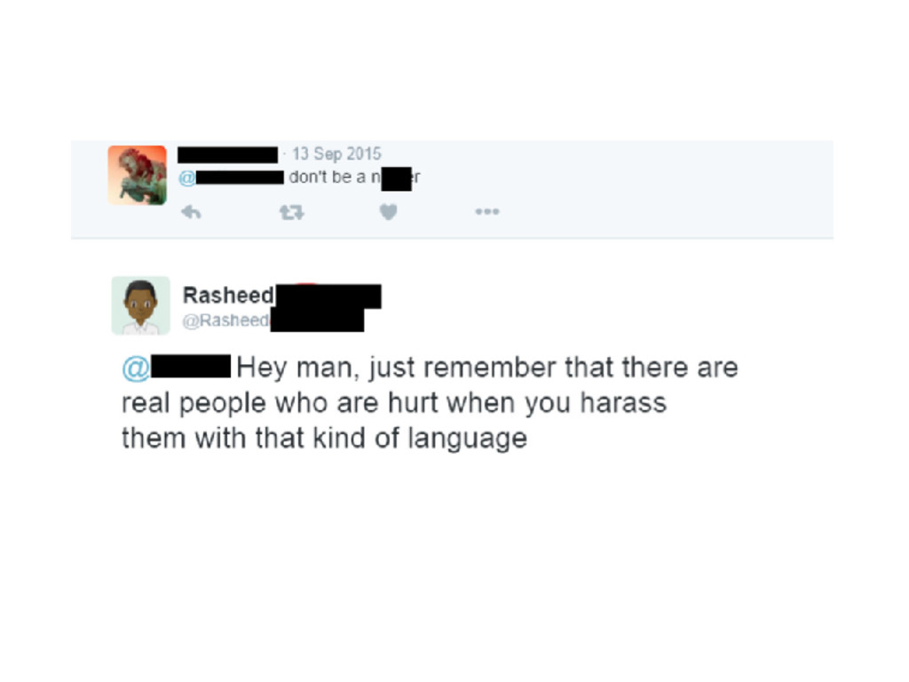
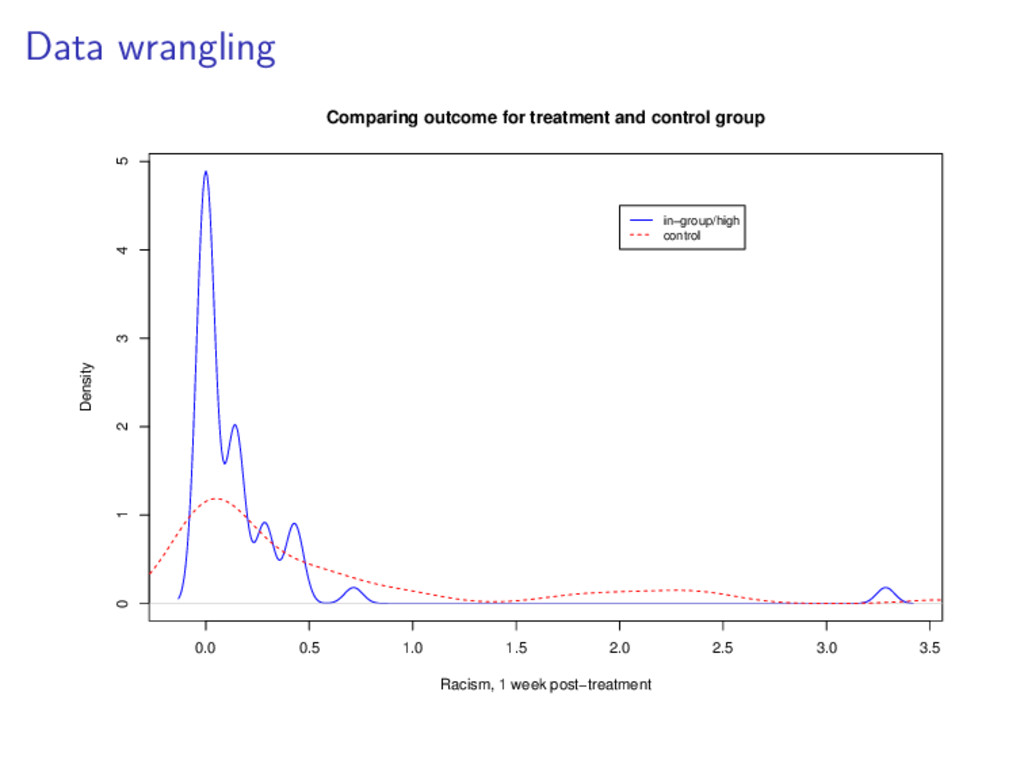
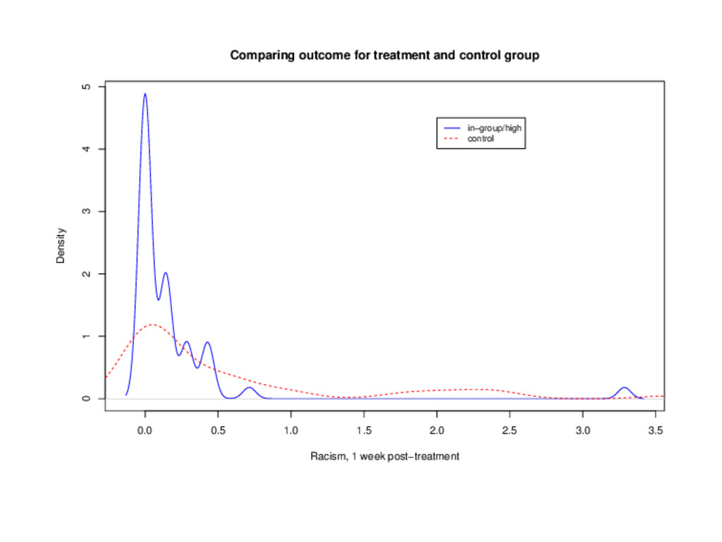
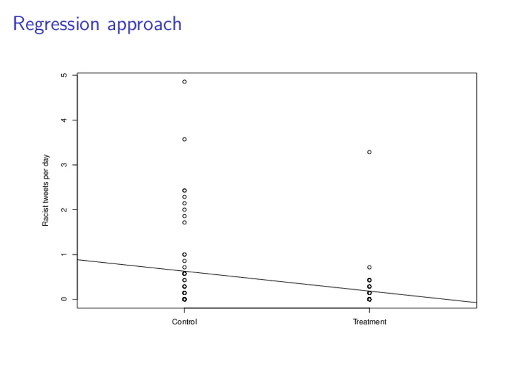
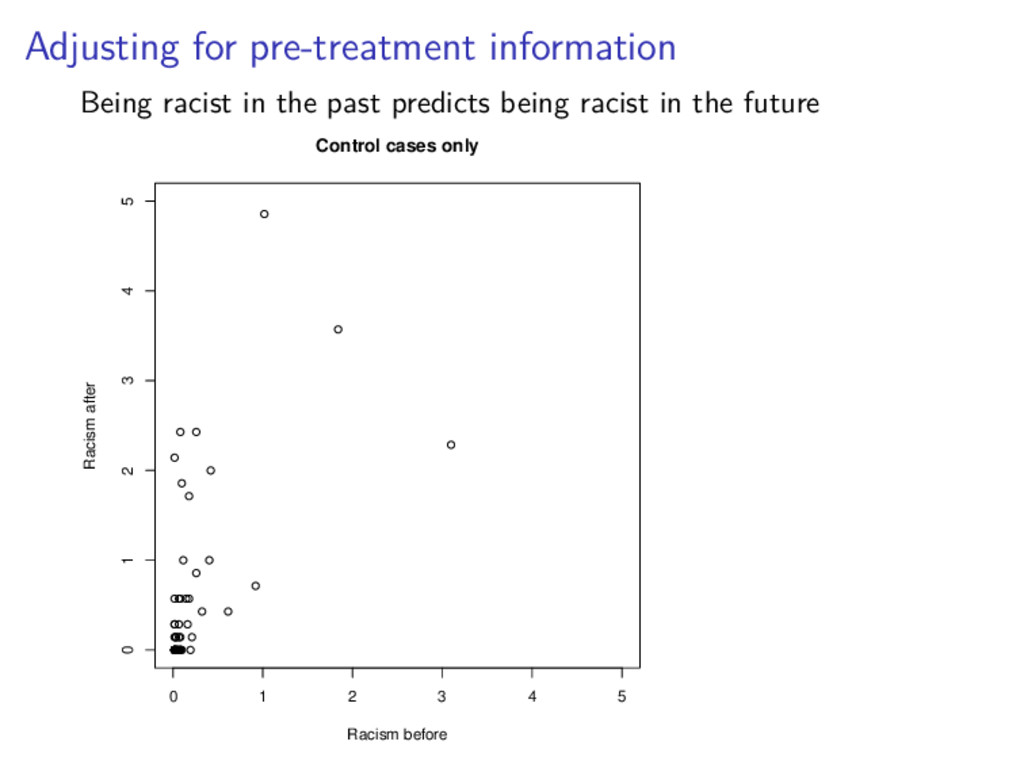
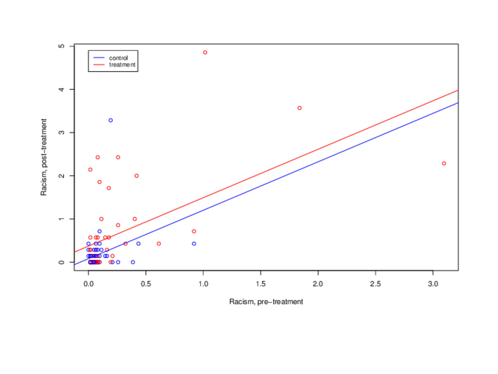
30. Data wrangling “Each panel shows the results of an OLS regression in which the dependent variable is the absolute number of instances of racists language during that period divided by the number of days in that time period.”
31. Data wrangling 0 1 2 3 4 5 6 7 10 11 12 13 14 15 16 17 18 19 23 24 25 34 0 20 40 60 80 100
32. Data wrangling control in−group/low out−group/low in−group/high out−group/high 0 1 2 3 4 5
33. Data wrangling munger.twogroup <- subset(munger, subset = treat.f %in% c(" dim(munger.twogroup) ## [1] 102 13
34. Data wrangling 0.0 0.5 1.0 1.5 2.0 2.5 3.0 3.5 0 1 2 3 4 5 Comparing outcome for treatment and control group Racism, 1 week post−treatment Density in−group/high control
35. Intermission What to make great plots without all the fiddling? Try ggplot2 at the COMPASS Workshop on December 7.
36. Intermission What to make great plots without all the fiddling? Try ggplot2 at the COMPASS Workshop on December 7. Can’t wait that long?
37. Intermission What to make great plots without all the fiddling? Try ggplot2 at the COMPASS Workshop on December 7. Can’t wait that long?
38. 0.0 0.5 1.0 1.5 2.0 2.5 3.0 3.5 0 1 2 3 4 5 Comparing outcome for treatment and control group Racism, 1 week post−treatment Density in−group/high control
39. Difference-of-means approach y.treat <- mean(munger[munger$treat.f == "in-group/high", " y.control <- mean(munger[munger$treat.f == "control", "raci est.ate <- y.treat - y.control print(paste("y.treat:", y.treat)) ## [1] "y.treat: 0.182857142857143" print(paste("y.control:", y.control)) ## [1] "y.control: 0.626373626373626" print(paste("est.ate:", est.ate)) ## [1] "est.ate: -0.443516483516483" The treated group created about 0.5 fewer racists post per day.
40. Difference-of-means approach n.treat <- sum(munger$treat.f == "in-group/high") n.control <- sum(munger$treat.f == "control") est.var.treat <- var(munger[munger$treat.f == "in-group/hig est.var.control <- var(munger[munger$treat.f == "control", est.se.ate <- sqrt(est.var.treat + est.var.control) print(paste("est.se.ate:", est.se.ate)) ## [1] "est.se.ate: 0.157452446428767"
41. Difference-of-means approach # 95% interval, rather than 1.96 you could use qnorm(0.975) lower.ci.95 <- est.ate - 1.96 * est.se.ate upper.ci.95 <- est.ate + 1.96 * est.se.ate print("Estimated 95 percent confidence interval:") ## [1] "Estimated 95 percent confidence interval:" print(c(lower.ci.95, upper.ci.95)) ## [1] -0.7521233 -0.1349097
42. Regression approach Let’s try that again with regression
43. Regression approach, data wrangling munger.subset <- subset(munger, subset = treat.f %in% c("control", "in-group/high")) munger.subset$treat.n <- NA cases.ih <- munger.subset$treat.f == "in-group/high" munger.subset[cases.ih, "treat.n"] <- 1 cases.c <- munger.subset$treat.f == "control" munger.subset[cases.c, "treat.n"] <- 0
44. Regression approach 0.0 0.2 0.4 0.6 0.8 1.0 0 1 2 3 4 5 munger.subset$treat.n munger.subset$racism.scores.post.1wk
45. Regression approach 0 1 2 3 4 5 Racist tweets per day Control Treatment
46. Regression approach 0 1 2 3 4 5 Racist tweets per day Control Treatment
47. fit <- lm(racism.scores.post.1wk ~ treat.n, data = munger.subset) ˆ yi = ˆ β0 + ˆ β1xi where ˆ yi racist tweets per day
48. fit <- lm(racism.scores.post.1wk ~ treat.n, data = munger.subset) ˆ yi = ˆ β0 + ˆ β1xi where ˆ yi racist tweets per day xi 1 if treatment, 0 if control
49. ## ## Call: ## lm(formula = racism.scores.post.1wk ~ treat.n, data = mu ## ## Coefficients: ## (Intercept) treat.n ## 0.6264 -0.4435 ## [1] "y.treat: 0.182857142857143" ## [1] "y.control: 0.626373626373626"
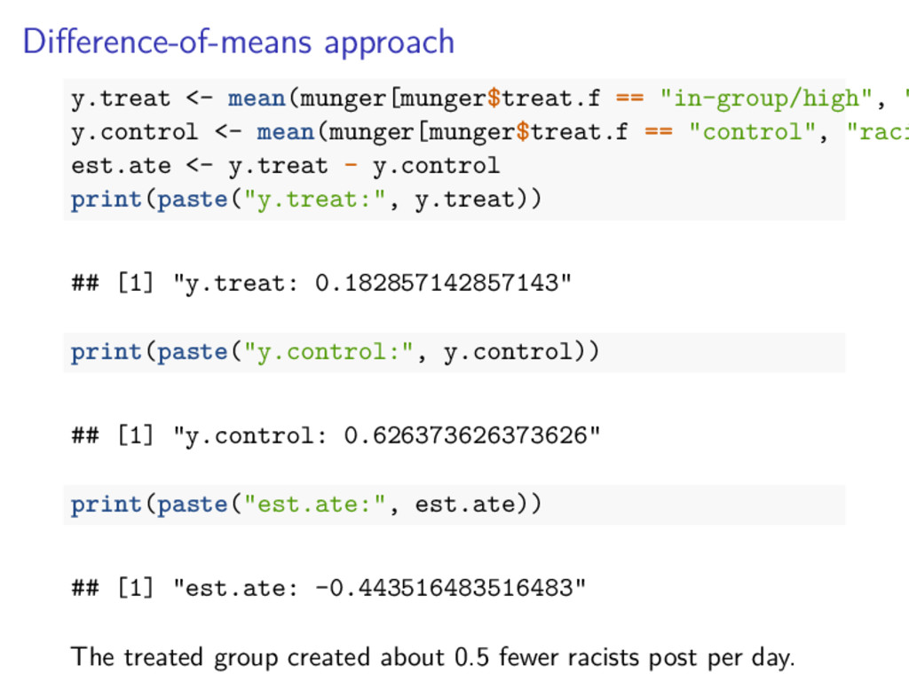
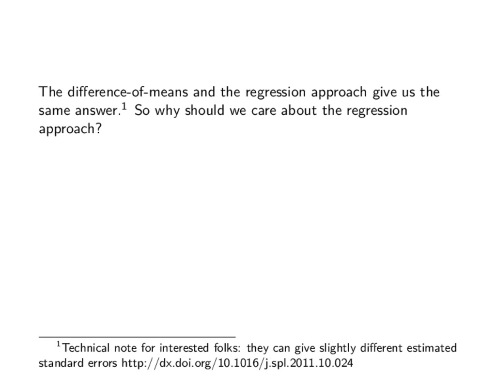
50. The difference-of-means and the regression approach give us the same answer.1 So why should we care about the regression approach? 1Technical note for interested folks: they can give slightly different estimated standard errors http://dx.doi.org/10.1016/j.spl.2011.10.024
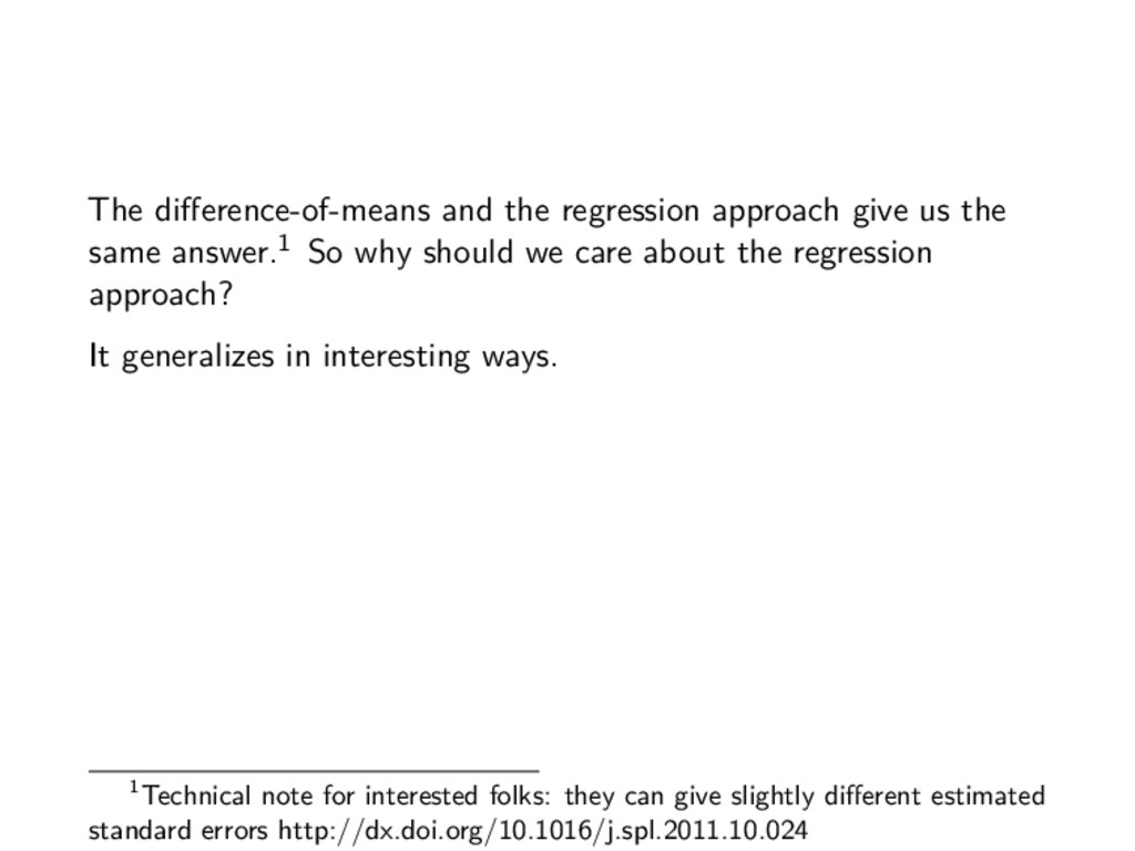
51. The difference-of-means and the regression approach give us the same answer.1 So why should we care about the regression approach? It generalizes in interesting ways. 1Technical note for interested folks: they can give slightly different estimated standard errors http://dx.doi.org/10.1016/j.spl.2011.10.024
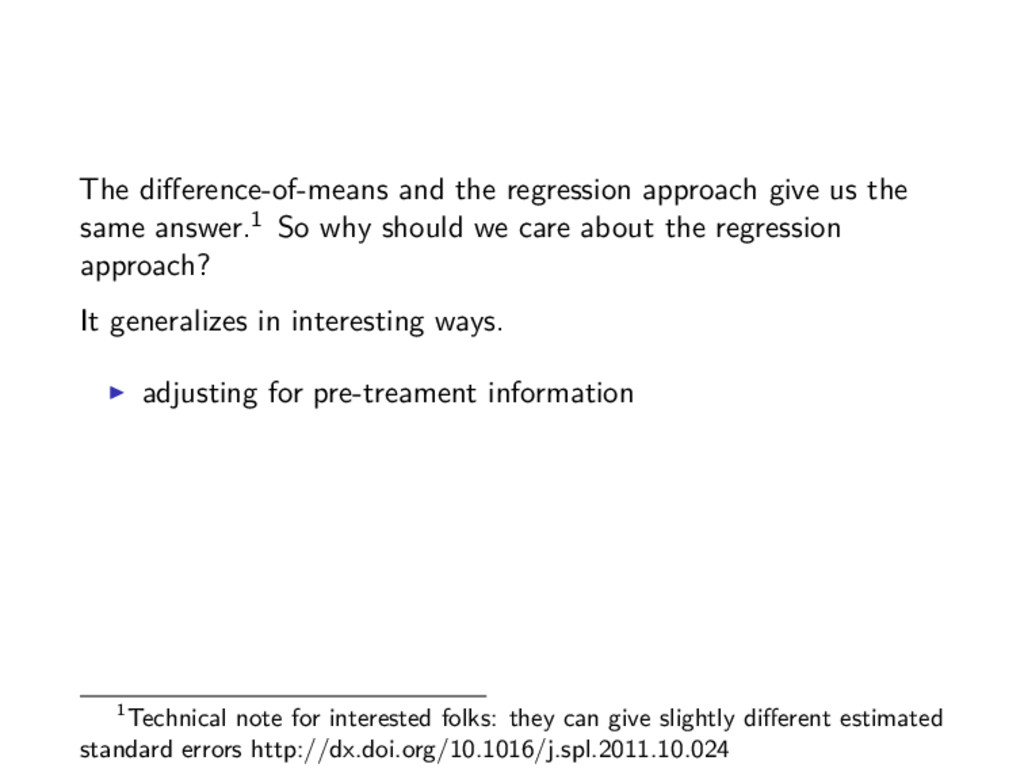
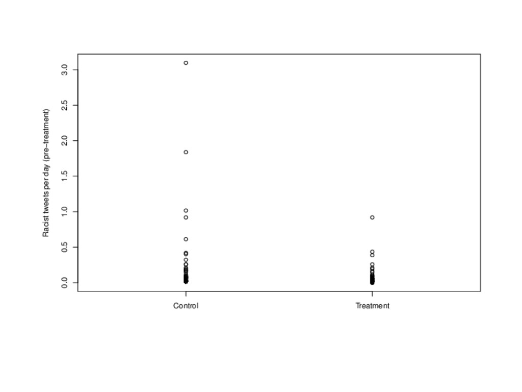
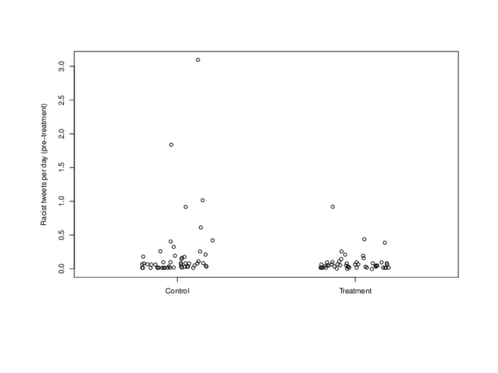
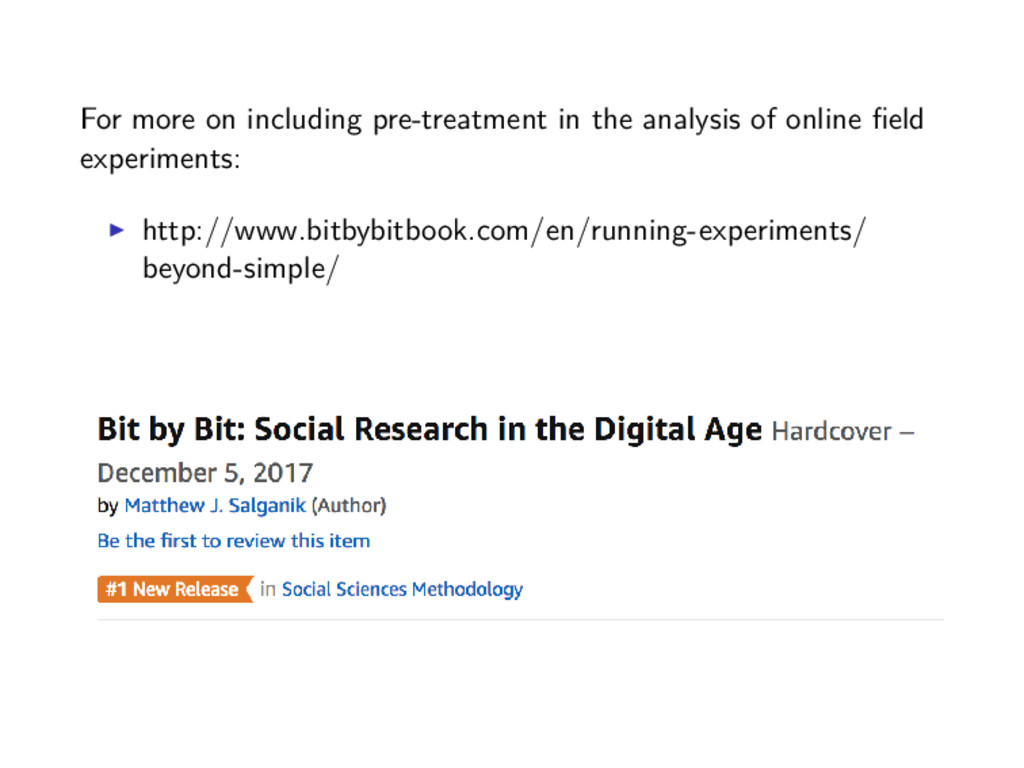
52. The difference-of-means and the regression approach give us the same answer.1 So why should we care about the regression approach? It generalizes in interesting ways. adjusting for pre-treament information 1Technical note for interested folks: they can give slightly different estimated standard errors http://dx.doi.org/10.1016/j.spl.2011.10.024
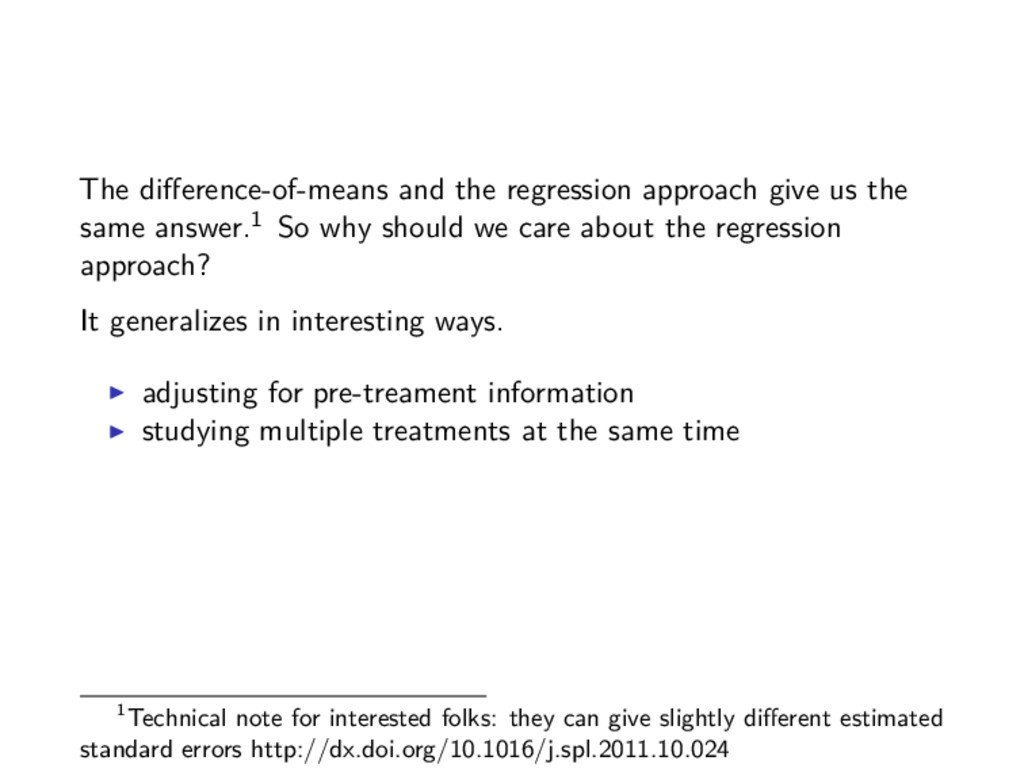
53. The difference-of-means and the regression approach give us the same answer.1 So why should we care about the regression approach? It generalizes in interesting ways. adjusting for pre-treament information studying multiple treatments at the same time 1Technical note for interested folks: they can give slightly different estimated standard errors http://dx.doi.org/10.1016/j.spl.2011.10.024
54. Adjusting for pre-treatment information Being racist in the past predicts being racist in the future 0 1 2 3 4 5 0 1 2 3 4 5 Control cases only Racism before Racism after
55. 0.0 0.5 1.0 1.5 2.0 2.5 3.0 Racist tweets per day (pre−treatment) Control Treatment
56. 0.0 0.5 1.0 1.5 2.0 2.5 3.0 Racist tweets per day (pre−treatment) Control Treatment
57. For more on including pre-treatment in the analysis of online field experiments: http://www.bitbybitbook.com/en/running-experiments/ beyond-simple/
58. For more on including pre-treatment in the analysis of online field experiments: http://www.bitbybitbook.com/en/running-experiments/ beyond-simple/ http://www.bitbybitbook.com/en/running-experiments/ exp-advice/3rs/
59. 0.0 0.5 1.0 1.5 2.0 2.5 3.0 0 1 2 3 4 5 Racism, pre−treatment Racism, post−treatment control treatment
60. fit1 <- lm(racism.scores.post.1wk ~ racism.scores.pre.2mon + treat.n, data = munger.subset) ˆ yi = ˆ β0 + ˆ β1xi,1 + ˆ β2xi,2 where ˆ yi racist tweets per day, post-treatment
61. fit1 <- lm(racism.scores.post.1wk ~ racism.scores.pre.2mon + treat.n, data = munger.subset) ˆ yi = ˆ β0 + ˆ β1xi,1 + ˆ β2xi,2 where ˆ yi racist tweets per day, post-treatment xi,1 racist tweets per day, pre-treatment
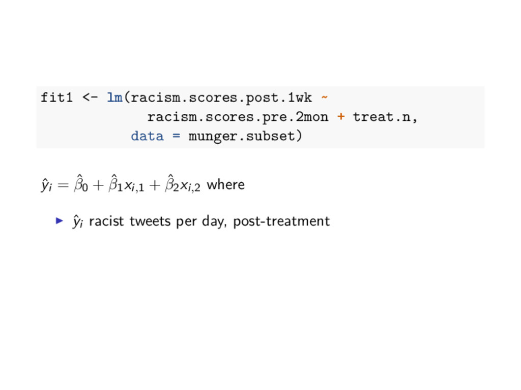
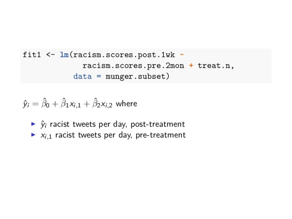
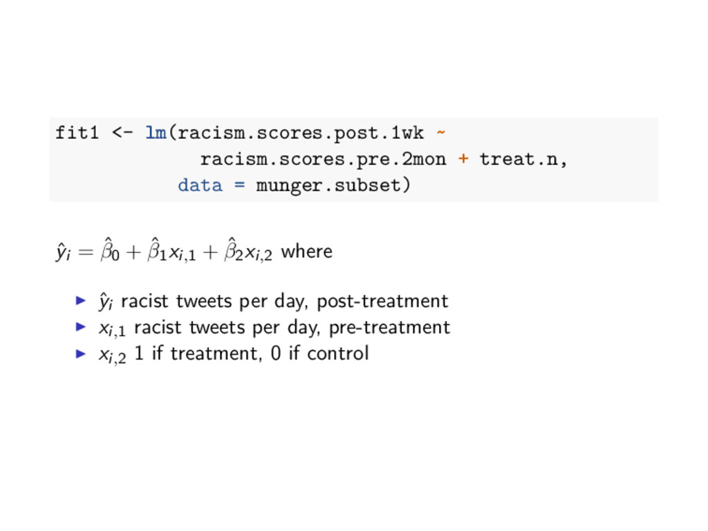
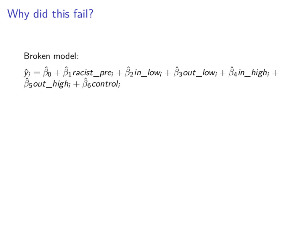
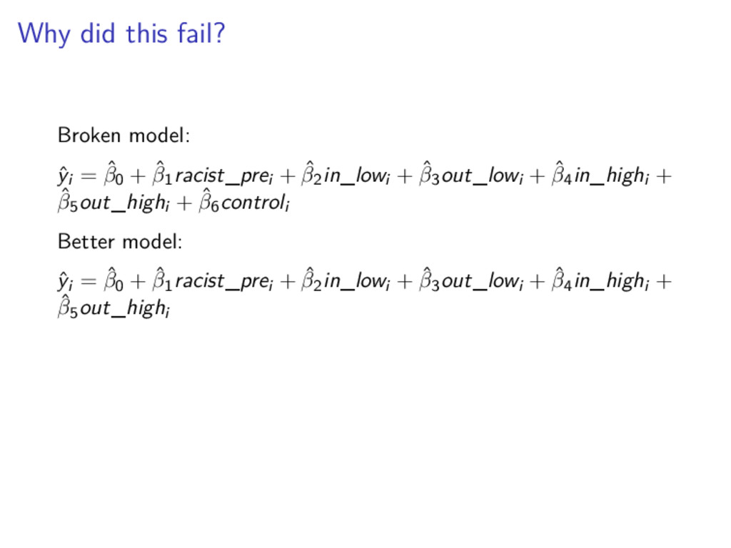
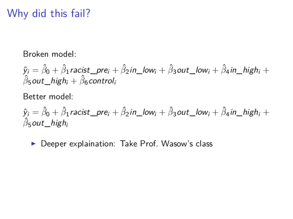
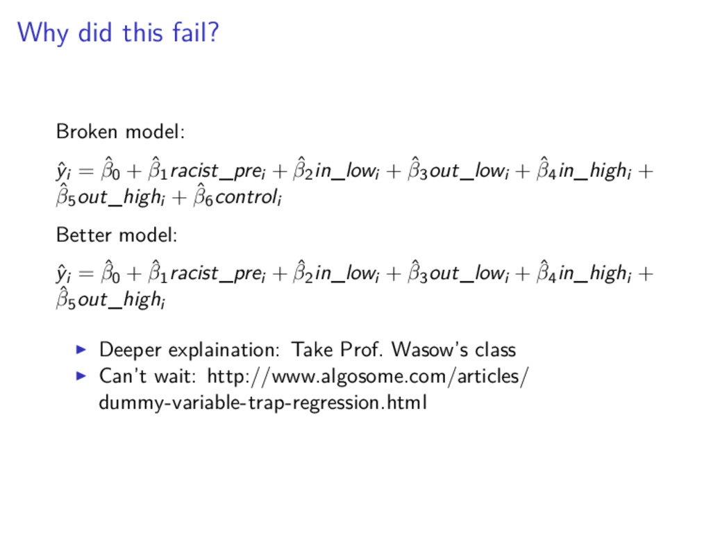
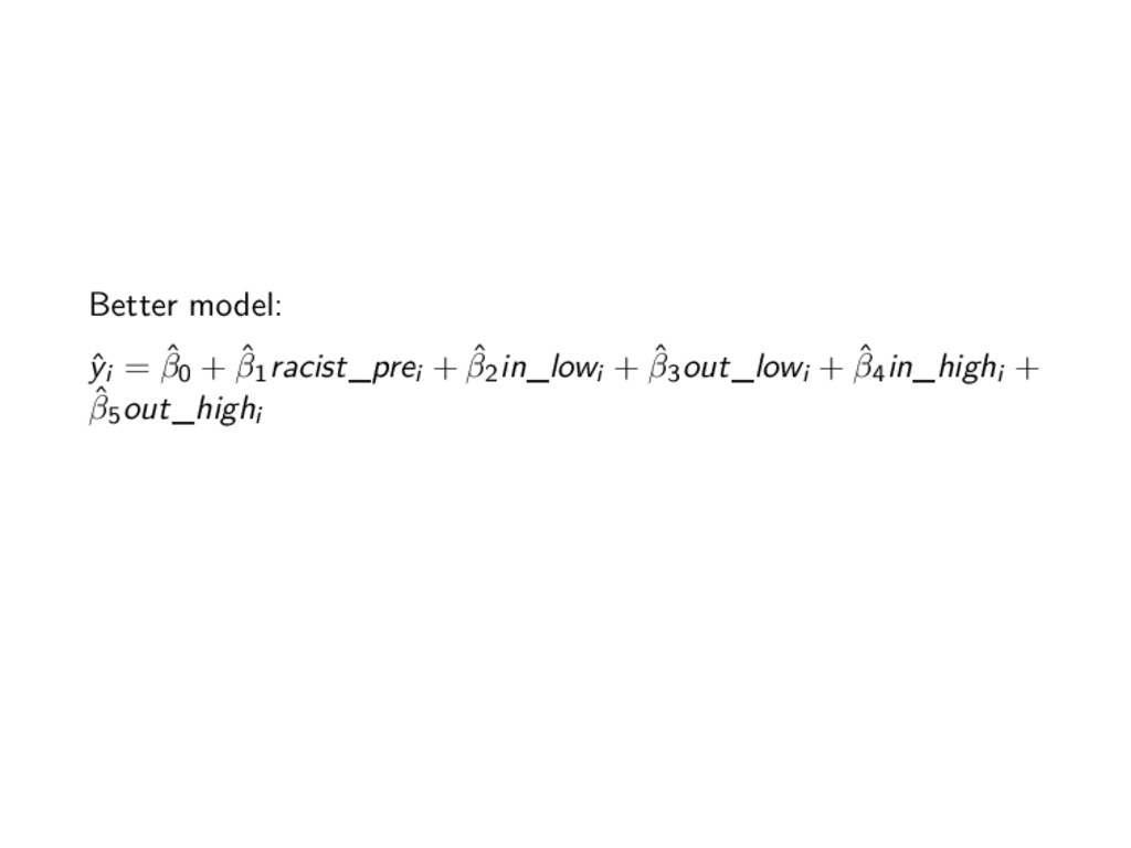
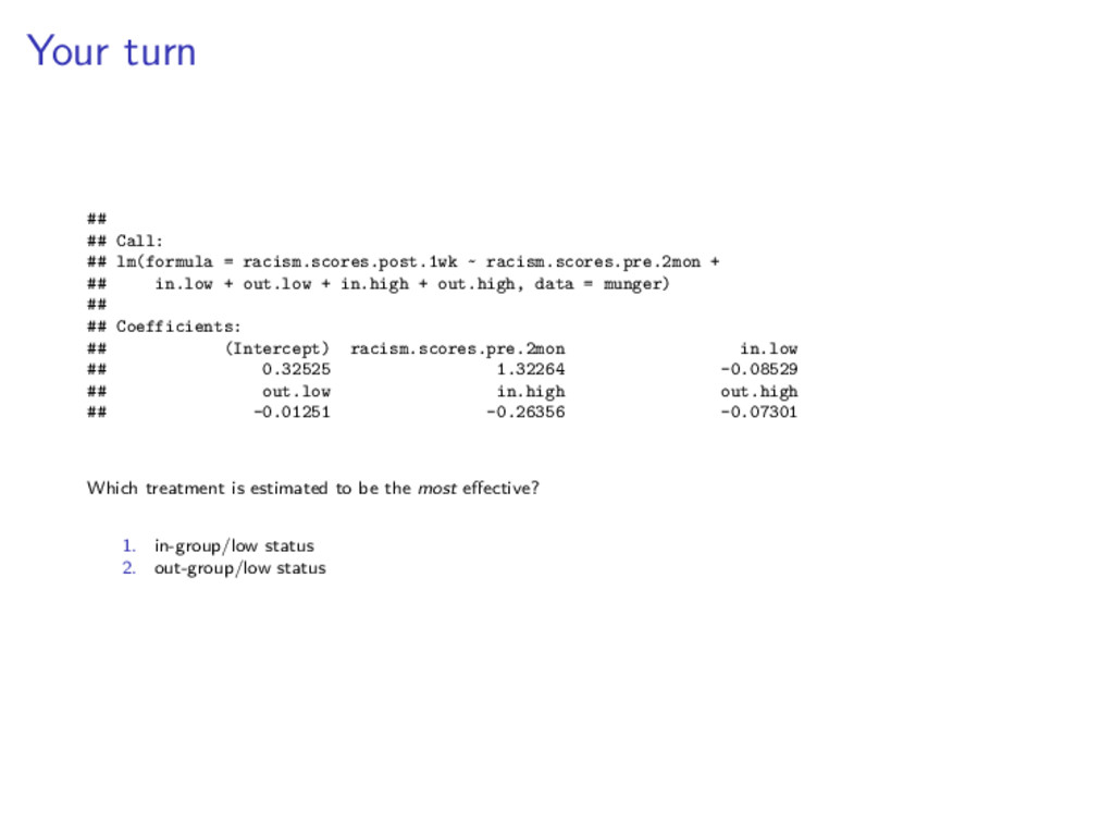
62. fit1 <- lm(racism.scores.post.1wk ~ racism.scores.pre.2mon + treat.n, data = munger.subset) ˆ yi = ˆ β0 + ˆ β1xi,1 + ˆ β2xi,2 where ˆ yi racist tweets per day, post-treatment xi,1 racist tweets per day, pre-treatment xi,2 1 if treatment, 0 if control
63. lm(racism.scores.post.1wk ~ racism.scores.pre.2mon + treat.n, data = munger.subset) ## ## Call: ## lm(formula = racism.scores.post.1wk ~ racism.scores.pre.2mon + ## treat.n, data = munger.subset) ## ## Coefficients: ## (Intercept) racism.scores.pre.2mon treat.n ## 0.3710 1.1219 -0.2909
64. lm(racism.scores.post.1wk ~ treat.n, data = munger.subset) ## ## Call: ## lm(formula = racism.scores.post.1wk ~ treat.n, data = mu ## ## Coefficients: ## (Intercept) treat.n ## 0.6264 -0.4435
65. adjusting for pre-treament information
66. adjusting for pre-treament information studying multiple treatments at the same time
67. Studying multiple treatments at the same time, data wrangling Creating dummy variable munger$control <- ifelse(munger$treat.f == "control", 1, 0) munger$in.low <- ifelse(munger$treat.f == "in-group/low", 1, 0) munger$out.low <- ifelse(munger$treat.f == "out-group/low", 1, 0) munger$in.high <- ifelse(munger$treat.f == "in-group/high", 1, 0) munger$out.high <- ifelse(munger$treat.f == "out-group/high 1, 0)
68. Studying multiple treatments at the same time, data wrangling head(munger[, c("treat.f", "control", "in.low", "out.low", "in.high", "out.high")] n = 10) ## treat.f control in.low out.low in.high out.high ## 1 out-group/high 0 0 0 0 1 ## 2 out-group/high 0 0 0 0 1 ## 3 out-group/high 0 0 0 0 1 ## 4 out-group/low 0 0 1 0 0 ## 5 out-group/low 0 0 1 0 0 ## 6 in-group/high 0 0 0 1 0 ## 7 in-group/high 0 0 0 1 0 ## 8 in-group/high 0 0 0 1 0 ## 9 in-group/low 0 1 0 0 0 ## 10 in-group/low 0 1 0 0 0
69. Studying multiple treatments at the same time lm(racism.scores.post.1wk ~ racism.scores.pre.2mon + in.low + out.low + in.high + out.high + control, data = munger) ## ## Call: ## lm(formula = racism.scores.post.1wk ~ racism.scores.pre. ## in.low + out.low + in.high + out.high + control, dat ## ## Coefficients: ## (Intercept) racism.scores.pre.2mon ## 0.32525 1.32264 ## out.low in.high ## -0.01251 -0.26356 ## control ## NA
70. Why did this fail? Broken model: ˆ yi = ˆ β0 + ˆ β1racist_prei + ˆ β2in_lowi + ˆ β3out_lowi + ˆ β4in_highi + ˆ β5out_highi + ˆ β6controli
71. Why did this fail? Broken model: ˆ yi = ˆ β0 + ˆ β1racist_prei + ˆ β2in_lowi + ˆ β3out_lowi + ˆ β4in_highi + ˆ β5out_highi + ˆ β6controli Better model: ˆ yi = ˆ β0 + ˆ β1racist_prei + ˆ β2in_lowi + ˆ β3out_lowi + ˆ β4in_highi + ˆ β5out_highi
72. Why did this fail? Broken model: ˆ yi = ˆ β0 + ˆ β1racist_prei + ˆ β2in_lowi + ˆ β3out_lowi + ˆ β4in_highi + ˆ β5out_highi + ˆ β6controli Better model: ˆ yi = ˆ β0 + ˆ β1racist_prei + ˆ β2in_lowi + ˆ β3out_lowi + ˆ β4in_highi + ˆ β5out_highi Deeper explaination: Take Prof. Wasow’s class
73. Why did this fail? Broken model: ˆ yi = ˆ β0 + ˆ β1racist_prei + ˆ β2in_lowi + ˆ β3out_lowi + ˆ β4in_highi + ˆ β5out_highi + ˆ β6controli Better model: ˆ yi = ˆ β0 + ˆ β1racist_prei + ˆ β2in_lowi + ˆ β3out_lowi + ˆ β4in_highi + ˆ β5out_highi Deeper explaination: Take Prof. Wasow’s class Can’t wait: http://www.algosome.com/articles/ dummy-variable-trap-regression.html
74. lm(racism.scores.post.1wk ~ racism.scores.pre.2mon + in.low + out.low + in.high + out.high, data = munger) ## ## Call: ## lm(formula = racism.scores.post.1wk ~ racism.scores.pre. ## in.low + out.low + in.high + out.high, data = munger ## ## Coefficients: ## (Intercept) racism.scores.pre.2mon ## 0.32525 1.32264 ## out.low in.high ## -0.01251 -0.26356
76. 0.0 0.5 1.0 1.5 2.0 2.5 3.0 0 1 2 3 4 5 Racism, pre−treatment Racism, post−treatment
77. Better model: ˆ yi = ˆ β0 + ˆ β1racist_prei + ˆ β2in_lowi + ˆ β3out_lowi + ˆ β4in_highi + ˆ β5out_highi
78. 0.0 0.5 1.0 1.5 2.0 2.5 3.0 0 1 2 3 4 5 Racism, pre−treatment Racism, post−treatment control in.low out.low in.high out.high.col
79. Your turn ## ## Call: ## lm(formula = racism.scores.post.1wk ~ racism.scores.pre.2mon + ## in.low + out.low + in.high + out.high, data = munger) ## ## Coefficients: ## (Intercept) racism.scores.pre.2mon in.low ## 0.32525 1.32264 -0.08529 ## out.low in.high out.high ## -0.01251 -0.26356 -0.07301 Which treatment is estimated to be the most effective? 1. in-group/low status
80. Your turn ## ## Call: ## lm(formula = racism.scores.post.1wk ~ racism.scores.pre.2mon + ## in.low + out.low + in.high + out.high, data = munger) ## ## Coefficients: ## (Intercept) racism.scores.pre.2mon in.low ## 0.32525 1.32264 -0.08529 ## out.low in.high out.high ## -0.01251 -0.26356 -0.07301 Which treatment is estimated to be the most effective? 1. in-group/low status 2. out-group/low status
81. Your turn ## ## Call: ## lm(formula = racism.scores.post.1wk ~ racism.scores.pre.2mon + ## in.low + out.low + in.high + out.high, data = munger) ## ## Coefficients: ## (Intercept) racism.scores.pre.2mon in.low ## 0.32525 1.32264 -0.08529 ## out.low in.high out.high ## -0.01251 -0.26356 -0.07301 Which treatment is estimated to be the most effective? 1. in-group/low status 2. out-group/low status 3. in-group/high status
82. Your turn ## ## Call: ## lm(formula = racism.scores.post.1wk ~ racism.scores.pre.2mon + ## in.low + out.low + in.high + out.high, data = munger) ## ## Coefficients: ## (Intercept) racism.scores.pre.2mon in.low ## 0.32525 1.32264 -0.08529 ## out.low in.high out.high ## -0.01251 -0.26356 -0.07301 Which treatment is estimated to be the most effective? 1. in-group/low status 2. out-group/low status 3. in-group/high status 4. out-group/high status
83. Your turn ## ## Call: ## lm(formula = racism.scores.post.1wk ~ racism.scores.pre.2mon + ## in.low + out.low + in.high + out.high, data = munger) ## ## Coefficients: ## (Intercept) racism.scores.pre.2mon in.low ## 0.32525 1.32264 -0.08529 ## out.low in.high out.high ## -0.01251 -0.26356 -0.07301 Which treatment is estimated to be the most effective? 1. in-group/low status 2. out-group/low status 3. in-group/high status 4. out-group/high status
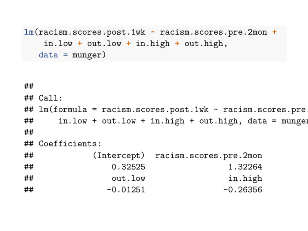
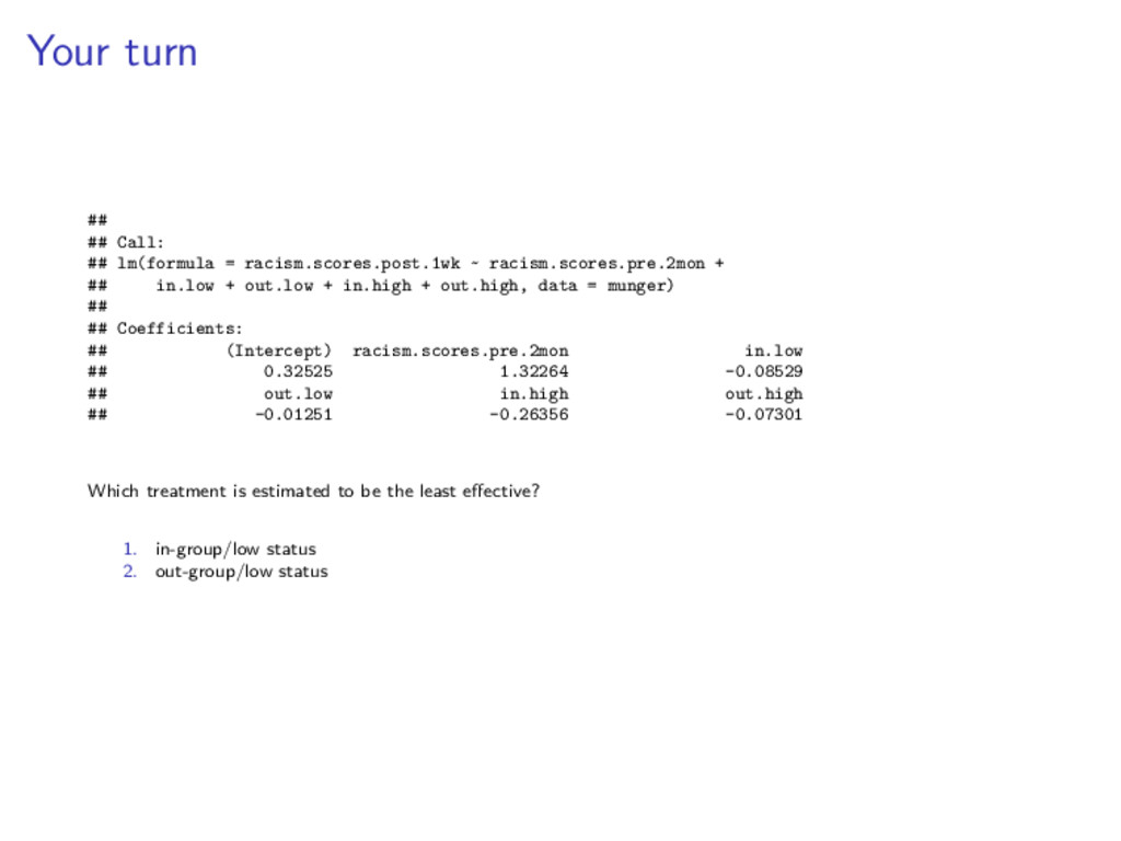
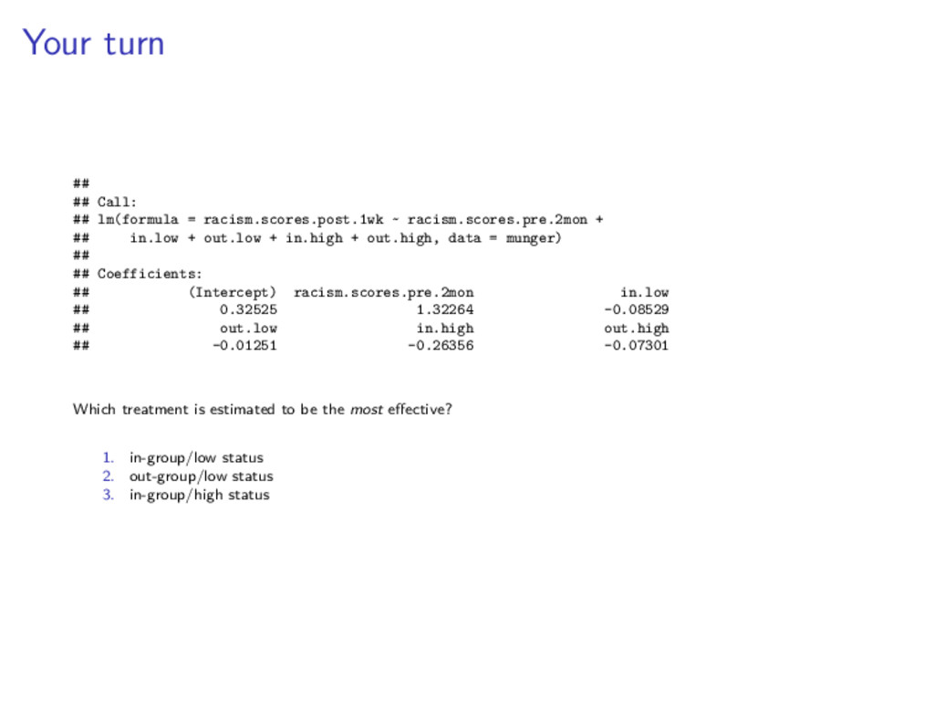
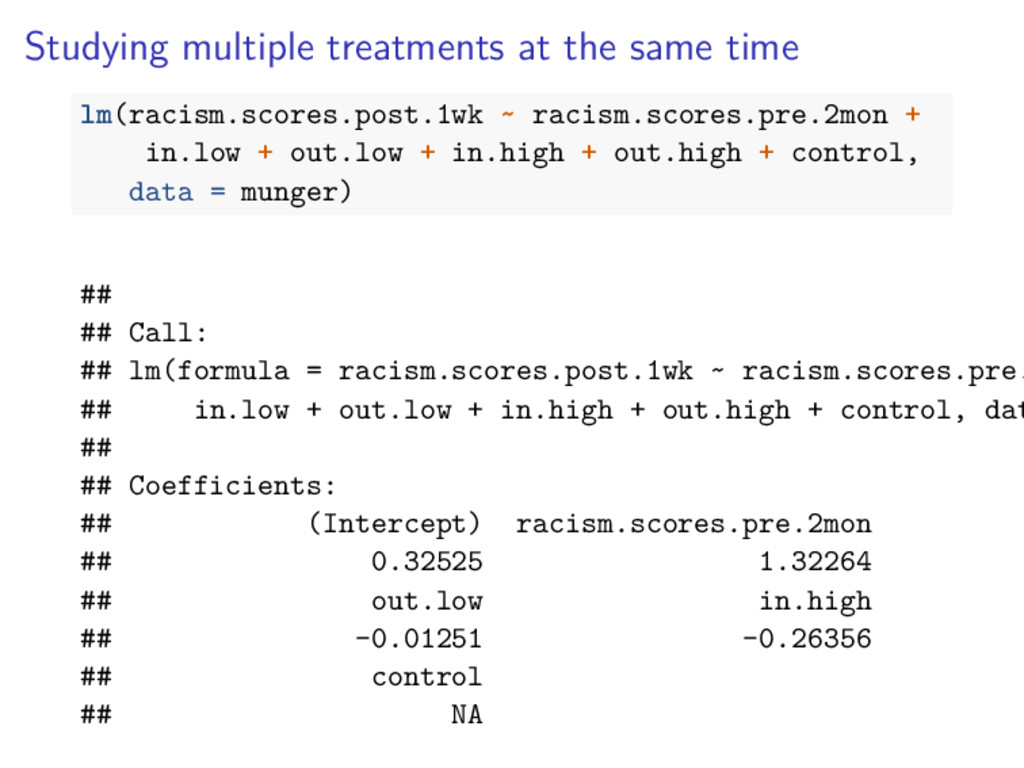
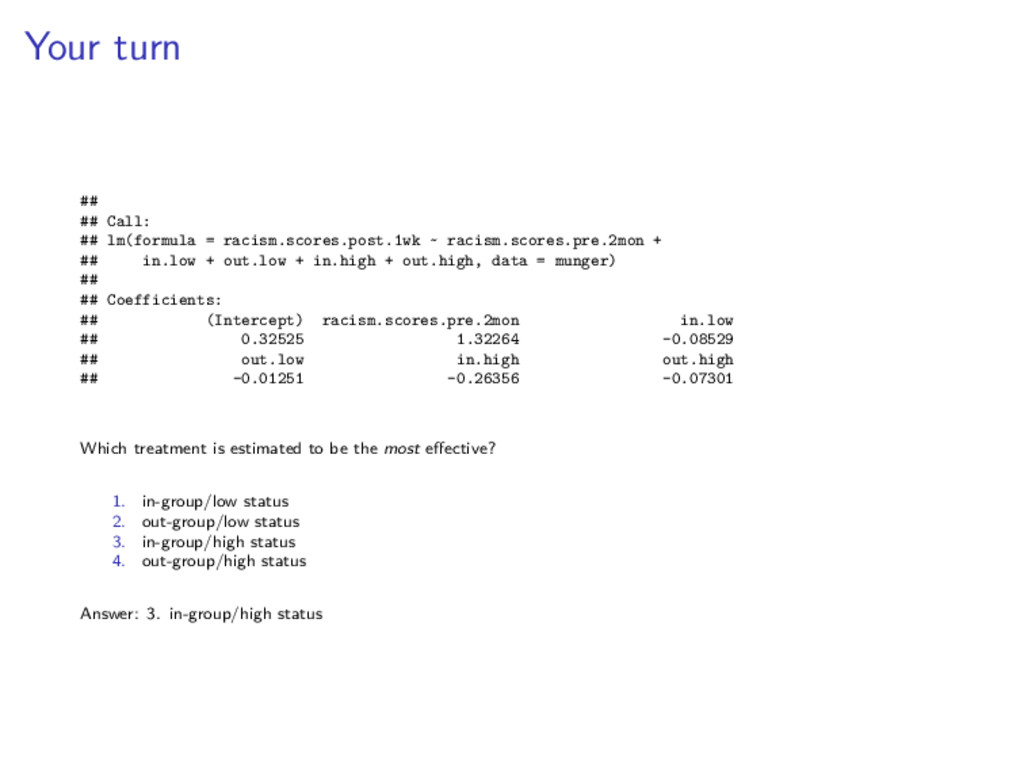
84. Your turn ## ## Call: ## lm(formula = racism.scores.post.1wk ~ racism.scores.pre.2mon + ## in.low + out.low + in.high + out.high, data = munger) ## ## Coefficients: ## (Intercept) racism.scores.pre.2mon in.low ## 0.32525 1.32264 -0.08529 ## out.low in.high out.high ## -0.01251 -0.26356 -0.07301 Which treatment is estimated to be the most effective? 1. in-group/low status 2. out-group/low status 3. in-group/high status 4. out-group/high status Answer: 3. in-group/high status
85. Your turn ## ## Call: ## lm(formula = racism.scores.post.1wk ~ racism.scores.pre.2mon + ## in.low + out.low + in.high + out.high, data = munger) ## ## Coefficients: ## (Intercept) racism.scores.pre.2mon in.low ## 0.32525 1.32264 -0.08529 ## out.low in.high out.high ## -0.01251 -0.26356 -0.07301 Which treatment is estimated to be the least effective? 1. in-group/low status
86. Your turn ## ## Call: ## lm(formula = racism.scores.post.1wk ~ racism.scores.pre.2mon + ## in.low + out.low + in.high + out.high, data = munger) ## ## Coefficients: ## (Intercept) racism.scores.pre.2mon in.low ## 0.32525 1.32264 -0.08529 ## out.low in.high out.high ## -0.01251 -0.26356 -0.07301 Which treatment is estimated to be the least effective? 1. in-group/low status 2. out-group/low status
87. Your turn ## ## Call: ## lm(formula = racism.scores.post.1wk ~ racism.scores.pre.2mon + ## in.low + out.low + in.high + out.high, data = munger) ## ## Coefficients: ## (Intercept) racism.scores.pre.2mon in.low ## 0.32525 1.32264 -0.08529 ## out.low in.high out.high ## -0.01251 -0.26356 -0.07301 Which treatment is estimated to be the least effective? 1. in-group/low status 2. out-group/low status 3. in-group/high status
88. Your turn ## ## Call: ## lm(formula = racism.scores.post.1wk ~ racism.scores.pre.2mon + ## in.low + out.low + in.high + out.high, data = munger) ## ## Coefficients: ## (Intercept) racism.scores.pre.2mon in.low ## 0.32525 1.32264 -0.08529 ## out.low in.high out.high ## -0.01251 -0.26356 -0.07301 Which treatment is estimated to be the least effective? 1. in-group/low status 2. out-group/low status 3. in-group/high status 4. out-group/high status
89. Your turn ## ## Call: ## lm(formula = racism.scores.post.1wk ~ racism.scores.pre.2mon + ## in.low + out.low + in.high + out.high, data = munger) ## ## Coefficients: ## (Intercept) racism.scores.pre.2mon in.low ## 0.32525 1.32264 -0.08529 ## out.low in.high out.high ## -0.01251 -0.26356 -0.07301 Which treatment is estimated to be the least effective? 1. in-group/low status 2. out-group/low status 3. in-group/high status 4. out-group/high status
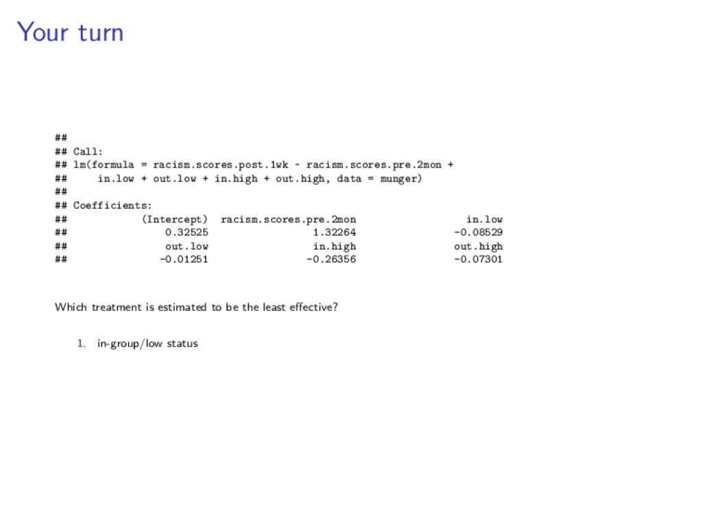
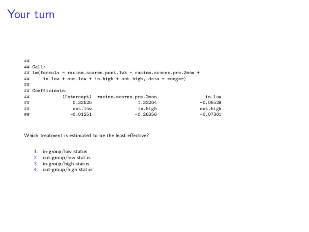
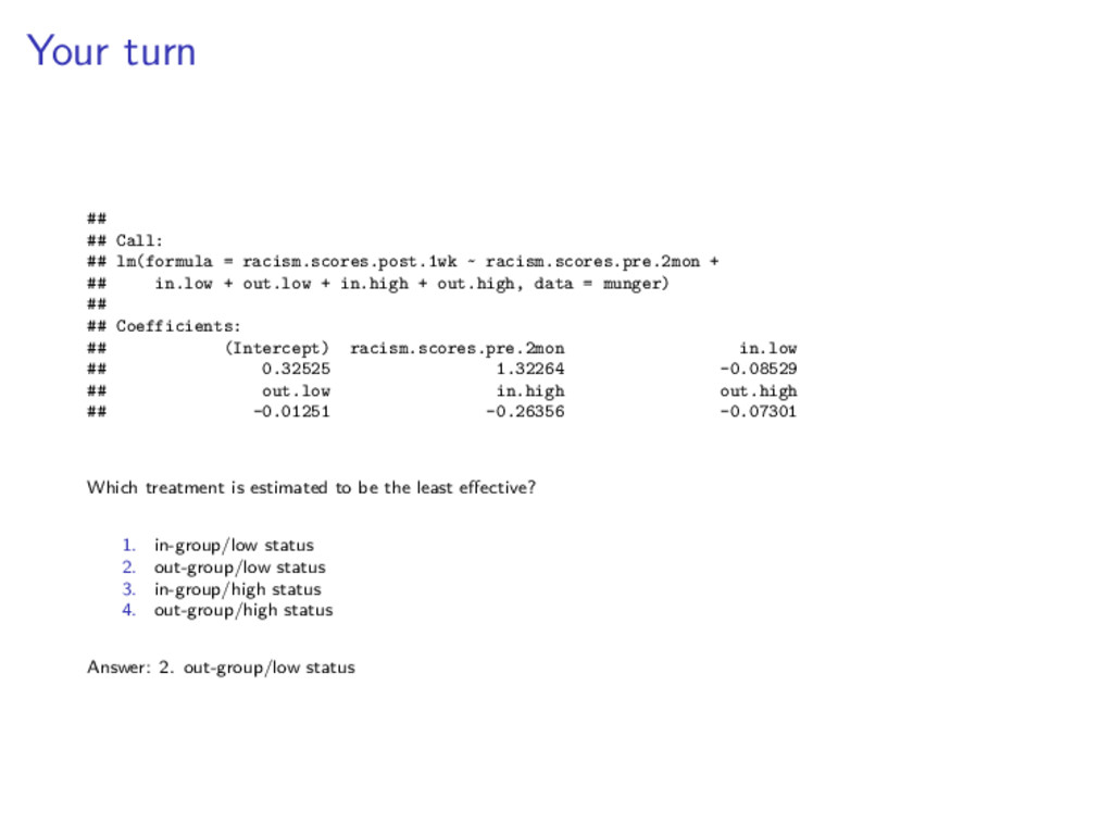
90. Your turn ## ## Call: ## lm(formula = racism.scores.post.1wk ~ racism.scores.pre.2mon + ## in.low + out.low + in.high + out.high, data = munger) ## ## Coefficients: ## (Intercept) racism.scores.pre.2mon in.low ## 0.32525 1.32264 -0.08529 ## out.low in.high out.high ## -0.01251 -0.26356 -0.07301 Which treatment is estimated to be the least effective? 1. in-group/low status 2. out-group/low status 3. in-group/high status 4. out-group/high status Answer: 2. out-group/low status
92. https://www.theatlantic.com/technology/archive/2017/10/ twitters-harassment-problem-is-baked-into-its-design/542952/
93. http://dx.doi.org/10.1007/s11109-016-9373-5
94. https://github.com/kmunger/ Replication-Materials-for-Tweetment-Effects-on-the-Tweeted}
95. Kevin Munger’s next project: Experimentally Reducing Partisan Incivility on Twitter paper: http://kmunger.github.io/pdfs/jmp.pdf
96. Kevin Munger’s next project: Experimentally Reducing Partisan Incivility on Twitter paper: http://kmunger.github.io/pdfs/jmp.pdf slides from talk at Twitter: http://kmunger.github.io/pdfs/munger_twitter_8_31.pdf
97. Goals for today See real data analyis workflow (with data wrangling)
98. Goals for today See real data analyis workflow (with data wrangling) Review difference-of-means
99. Goals for today See real data analyis workflow (with data wrangling) Review difference-of-means Show connection between difference-of-means and regression
100. Goals for today See real data analyis workflow (with data wrangling) Review difference-of-means Show connection between difference-of-means and regression Explore multiple regression with continuous and dummy variables in equations, code, pictures, and words
101. Goals for today See real data analyis workflow (with data wrangling) Review difference-of-means Show connection between difference-of-means and regression Explore multiple regression with continuous and dummy variables in equations, code, pictures, and words Learn something about Twitter
102. But there are open questions 0.0 0.5 1.0 1.5 2.0 2.5 3.0 0 1 2 3 4 5 Racism, pre−treatment Racism, post−treatment control in.low out.low in.high out.high.col What if the effect of the treatment varies based on the amount of racist speech pre-treatment?
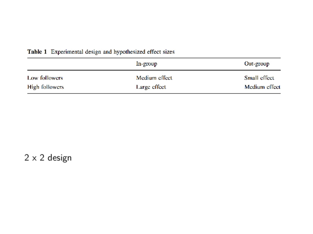
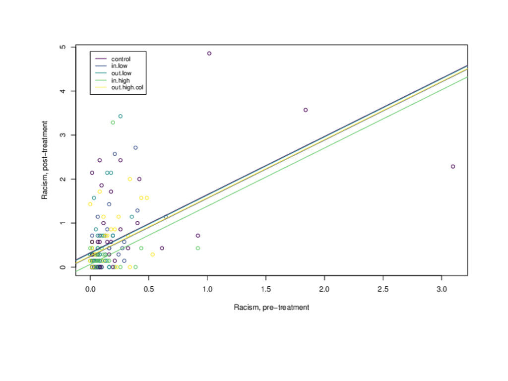
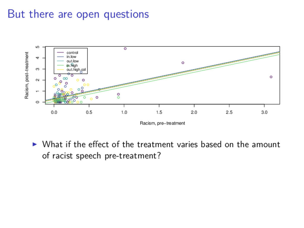
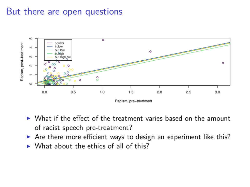
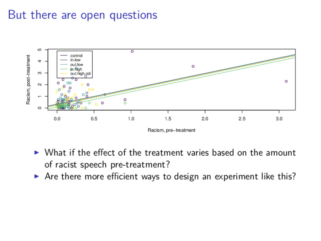
103. But there are open questions 0.0 0.5 1.0 1.5 2.0 2.5 3.0 0 1 2 3 4 5 Racism, pre−treatment Racism, post−treatment control in.low out.low in.high out.high.col What if the effect of the treatment varies based on the amount of racist speech pre-treatment? Are there more efficient ways to design an experiment like this?
104. But there are open questions 0.0 0.5 1.0 1.5 2.0 2.5 3.0 0 1 2 3 4 5 Racism, pre−treatment Racism, post−treatment control in.low out.low in.high out.high.col What if the effect of the treatment varies based on the amount of racist speech pre-treatment? Are there more efficient ways to design an experiment like this? What about the ethics of all of this?
105. SOC 412: Designing Field Experiments at Scale Online platforms, which monitor and intervene in the lives of billions of people, routinely host thousands of experiments to evaluate policies, test products, and contribute to theory in the social sciences. These experiments are also powerful tools to monitor injustice and govern human and algorithm behavior. How can we do field experiments at scale, reliably, and ethically?
106. SOC 412: Designing Field Experiments at Scale By the end of the semester, you will be able to: Design, conduct, and interpret a novel online field experiment Syllabus: http://natematias.com/courses/soc412/syllabus.html
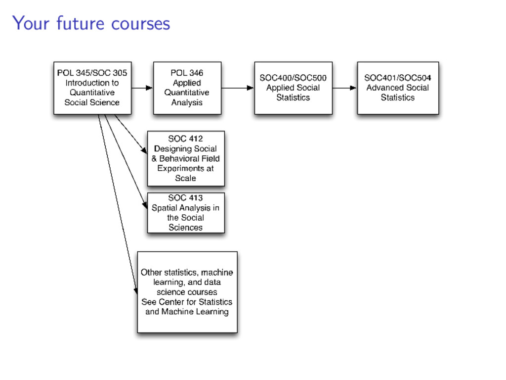
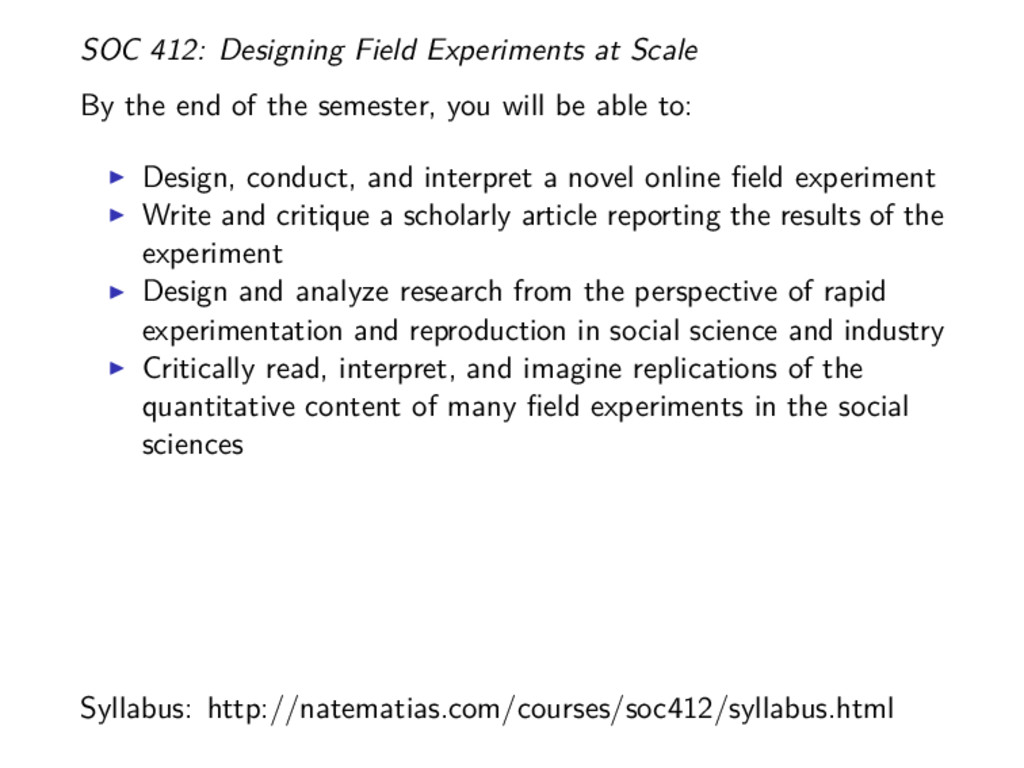
107. SOC 412: Designing Field Experiments at Scale By the end of the semester, you will be able to: Design, conduct, and interpret a novel online field experiment Write and critique a scholarly article reporting the results of the experiment Syllabus: http://natematias.com/courses/soc412/syllabus.html
108. SOC 412: Designing Field Experiments at Scale By the end of the semester, you will be able to: Design, conduct, and interpret a novel online field experiment Write and critique a scholarly article reporting the results of the experiment Design and analyze research from the perspective of rapid experimentation and reproduction in social science and industry Syllabus: http://natematias.com/courses/soc412/syllabus.html
109. SOC 412: Designing Field Experiments at Scale By the end of the semester, you will be able to: Design, conduct, and interpret a novel online field experiment Write and critique a scholarly article reporting the results of the experiment Design and analyze research from the perspective of rapid experimentation and reproduction in social science and industry Critically read, interpret, and imagine replications of the quantitative content of many field experiments in the social sciences Syllabus: http://natematias.com/courses/soc412/syllabus.html
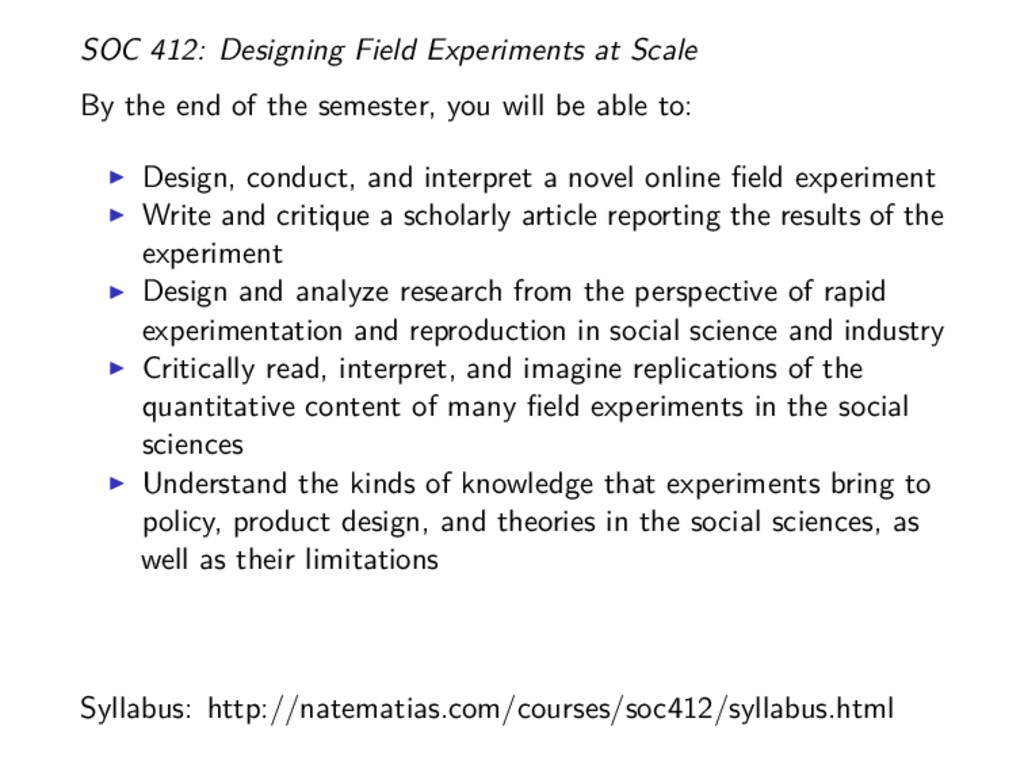
110. SOC 412: Designing Field Experiments at Scale By the end of the semester, you will be able to: Design, conduct, and interpret a novel online field experiment Write and critique a scholarly article reporting the results of the experiment Design and analyze research from the perspective of rapid experimentation and reproduction in social science and industry Critically read, interpret, and imagine replications of the quantitative content of many field experiments in the social sciences Understand the kinds of knowledge that experiments bring to policy, product design, and theories in the social sciences, as well as their limitations Syllabus: http://natematias.com/courses/soc412/syllabus.html
111. SOC 412: Designing Field Experiments at Scale By the end of the semester, you will be able to: Design, conduct, and interpret a novel online field experiment Write and critique a scholarly article reporting the results of the experiment Design and analyze research from the perspective of rapid experimentation and reproduction in social science and industry Critically read, interpret, and imagine replications of the quantitative content of many field experiments in the social sciences Understand the kinds of knowledge that experiments bring to policy, product design, and theories in the social sciences, as well as their limitations Engage with debates on the ethics and politics of experiments in your own work Syllabus: http://natematias.com/courses/soc412/syllabus.html
113. Logistics QSS assignments due 24 hours before precept
114. Logistics QSS assignments due 24 hours before precept Pset 3 will be posted W 12/6 and due W 12/13
115. Logistics QSS assignments due 24 hours before precept Pset 3 will be posted W 12/6 and due W 12/13 COMPASS workshop: Thurs, 11/30 Text Mining in R (Ethan)