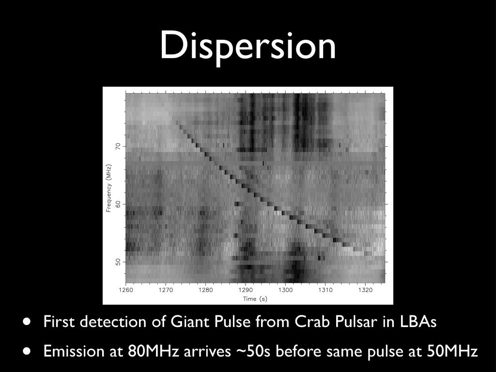
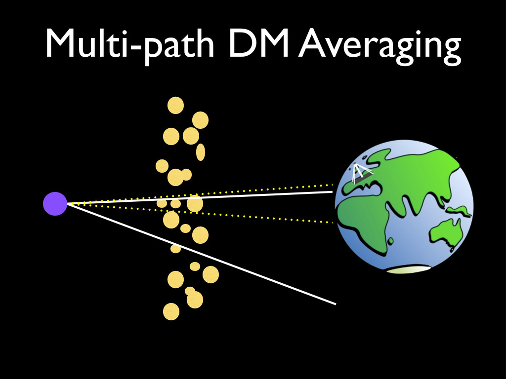
Malofeev 1985, Kuz’min 1986 and Shitov et al 1988 • Disputed by Phillips and Wolszczan 1998 • Recent paper by Cordes & Shannon gives a list of possible delays caused by ISM with steep frequency dependences...
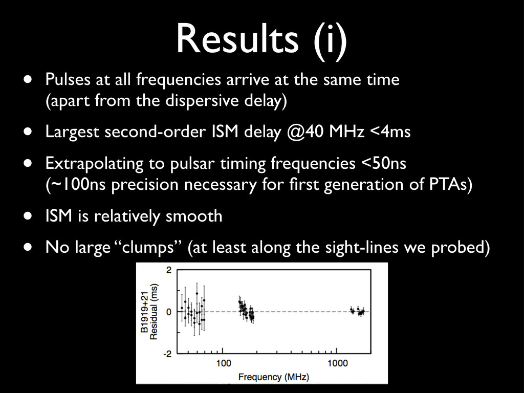
same time (apart from the dispersive delay) • Largest second-order ISM delay @40 MHz <4ms • Extrapolating to pulsar timing frequencies <50ns (~100ns precision necessary for first generation of PTAs) • ISM is relatively smooth • No large “clumps” (at least along the sight-lines we probed)
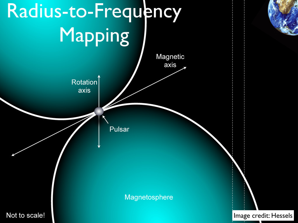
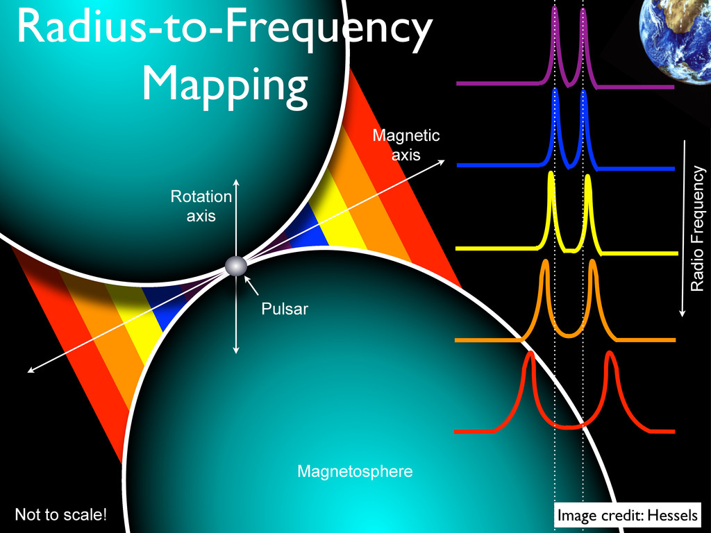
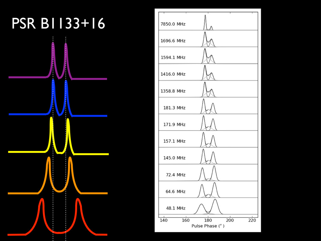
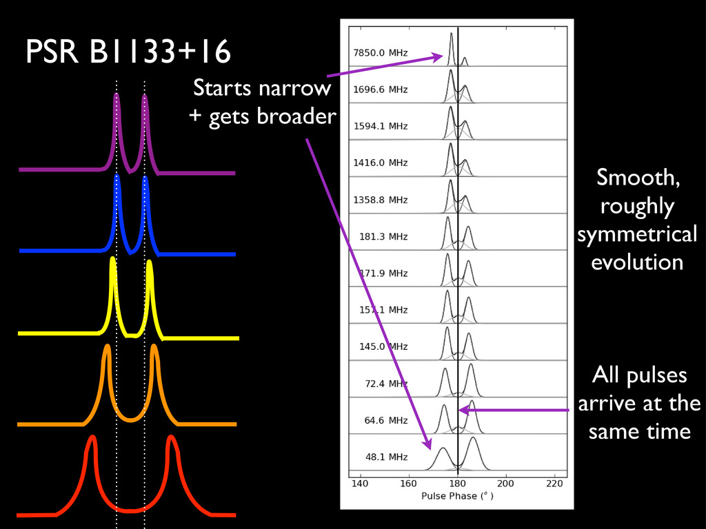
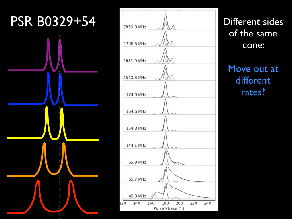
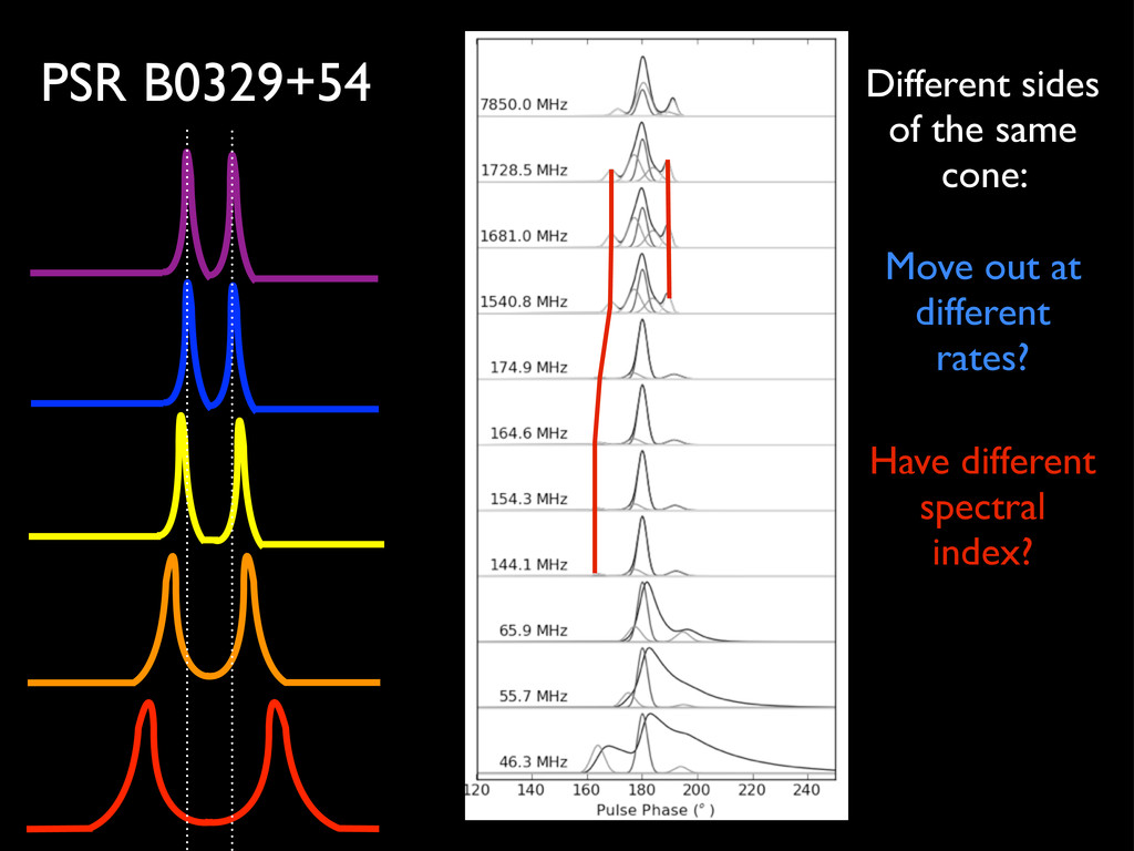
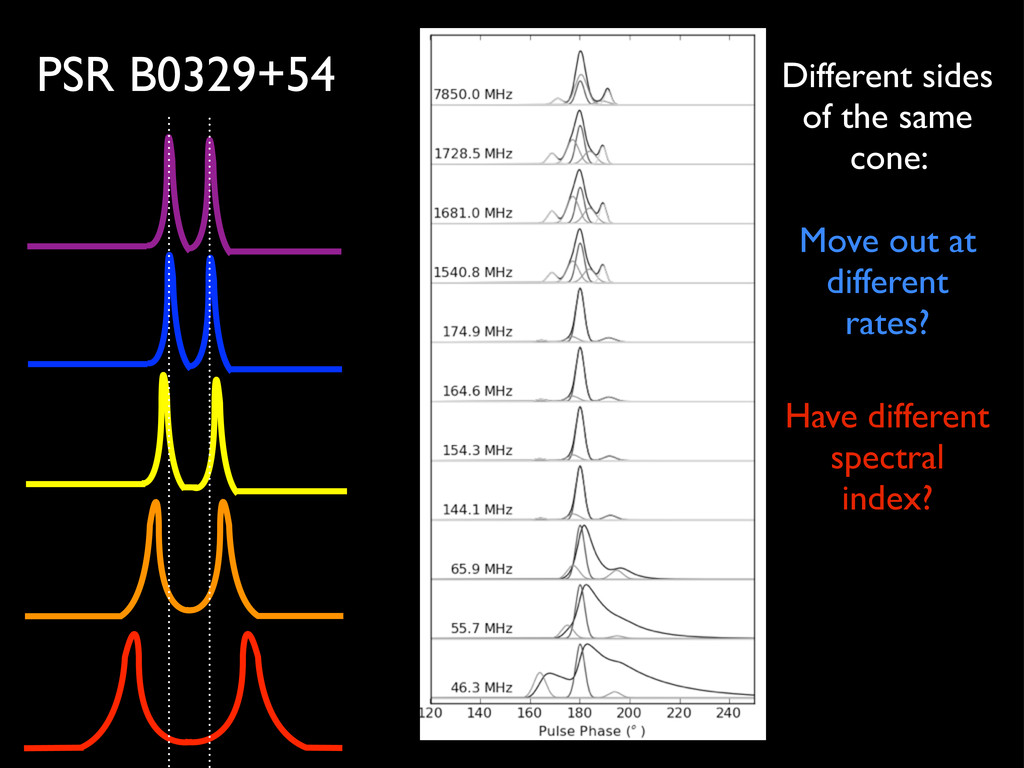
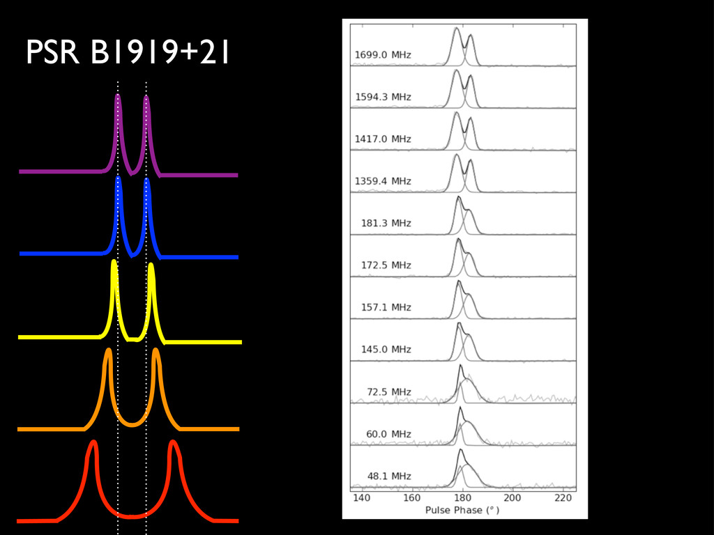
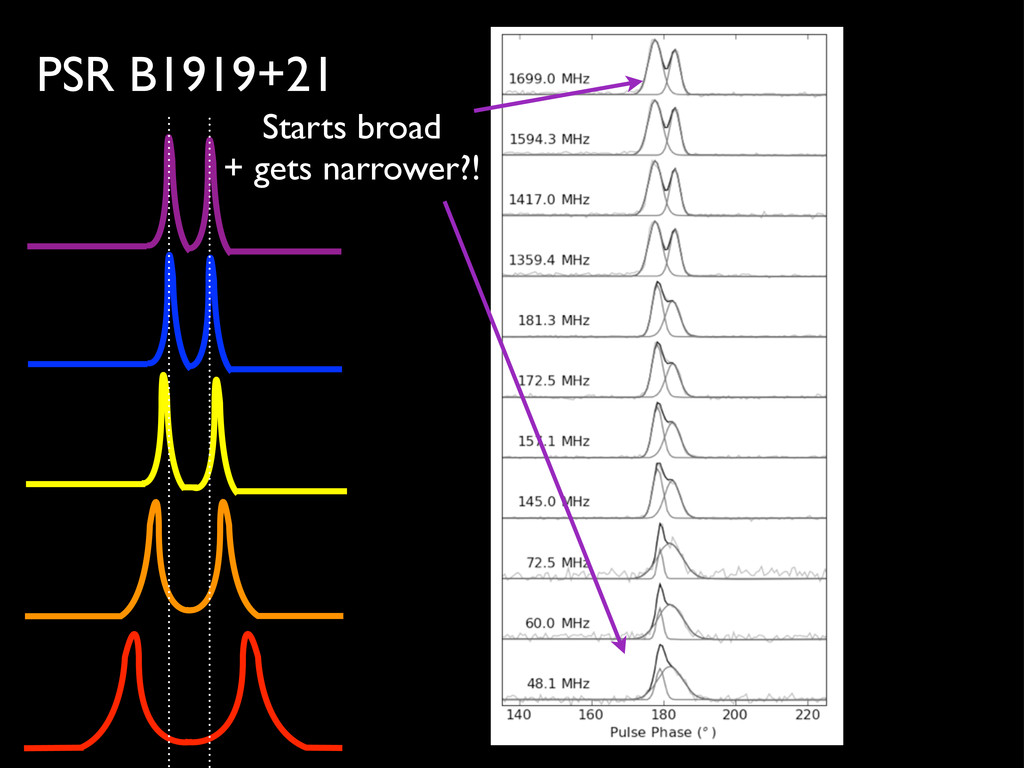
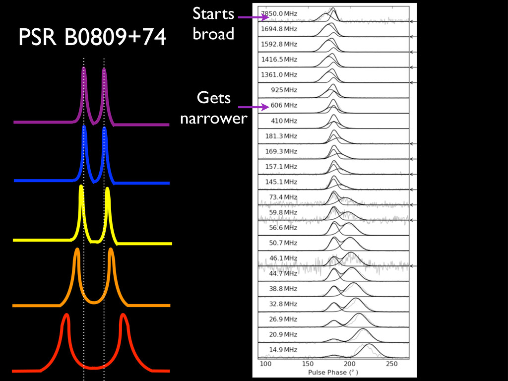
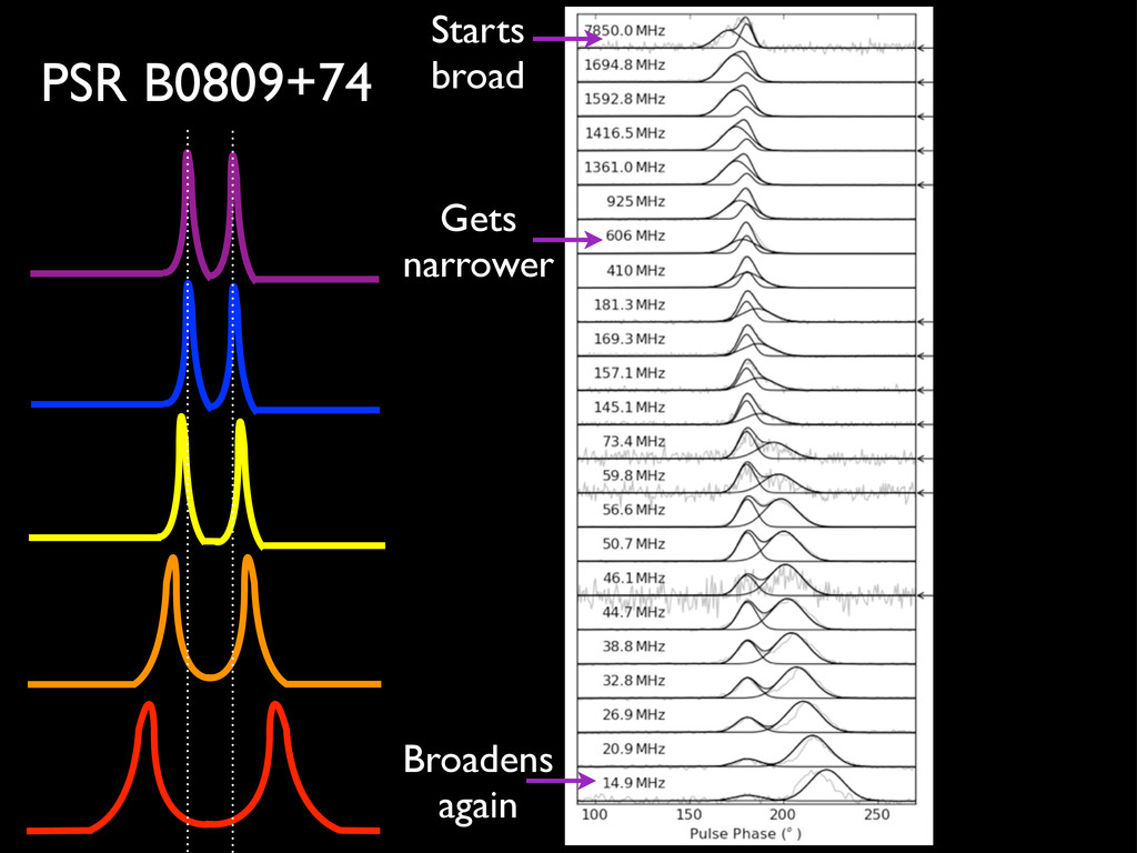
between 925 and 328 MHz (Gould & Lyne 1998; Edwards & Stappers 2003b), and LOFAR polarisation profile at 136 MHz (black lines) plotted along with the Stokes I profiles at each frequency (grey lines). The polarised com- ponent moves from the position of the leading component of the profile towards later pulse longitudes, tracing the broad component of the pulse profile. The width of the conal components as a function of fre- quency has been a subject of interest in the past. Mitra & Rankin (2002) found that the component widths remain constant be- tween 40 and 3000 MHz. We also see evidence of this in our model above 80 MHz, although the component widths begin to broaden below this value. Mitra & Rankin (2002) also no- ticed this broadening, and attributed it to dispersive smearing across a frequency channel or scattering from the ISM. In our observations, the dispersive smearing at 48 MHz (across a sin- gle 12 kHz channel) is 1.5o, which is enough to explain the observed broadening in the profile10. However, even disregard- ing this low frequency broadening Mitra & Rankin (2002) found that the spacing between the components between 100 MHz and 10 GHz changes too rapidly to be caused by a dipolar magnetic field. PSR B1133+16 is the pulsar which is most consistent with radius-to-frequency mapping of all the pulsars in our sample. However, in Section 6 we showed that its emission is confined to a very narrow region in the magnetosphere (<59 km) which is incompatible with the standard radius-to-frequency model. Radius-to-frequency mapping assumes that the emission at a given emission height traces the last open field line in the pulsar magnetosphere. From geometrical arguments (see for example Lorimer & Kramer 2005) it is possible to write the opening an- 10 The half power width of component 1 increases from 1.9o at 72 MHz to 3.6o at 48 MHz, and component 2 increases from 2.1o at 72 MHz to 3.4o at 48 MHz.
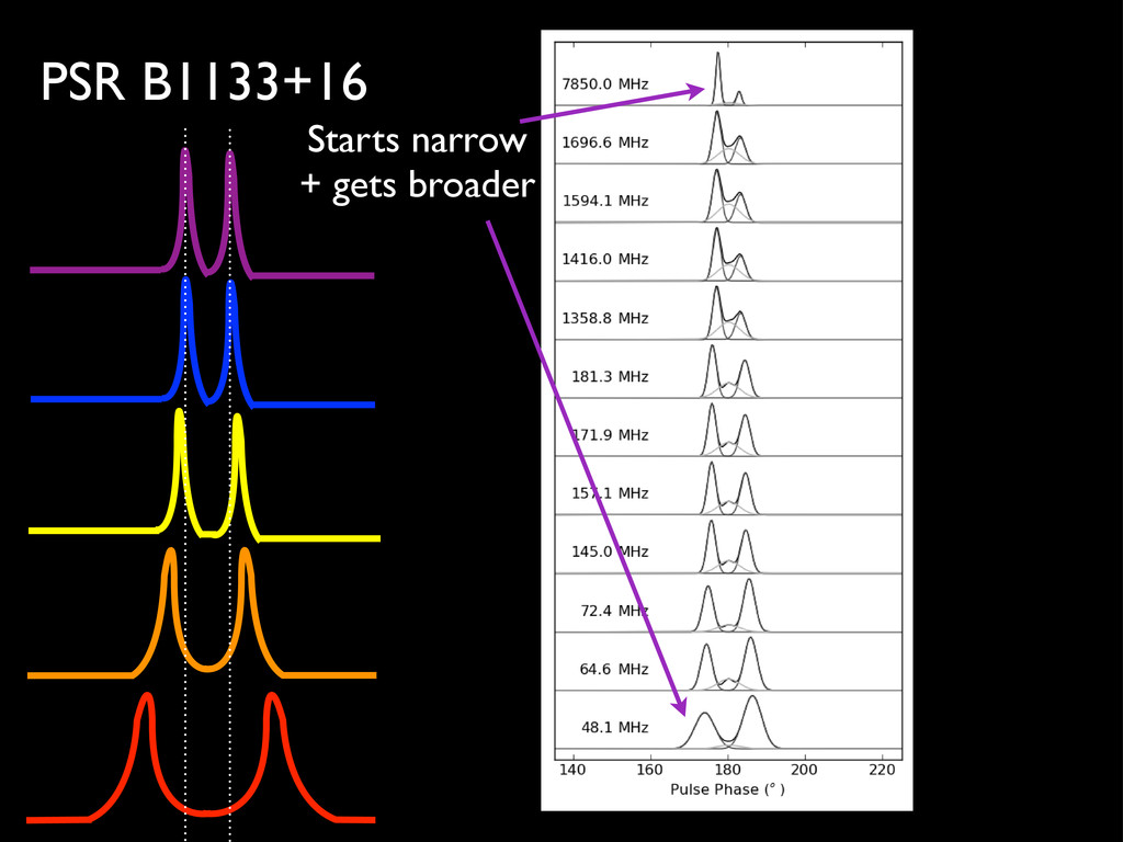
between 925 and 328 MHz (Gould & Lyne 1998; Edwards & Stappers 2003b), and LOFAR polarisation profile at 136 MHz (black lines) plotted along with the Stokes I profiles at each frequency (grey lines). The polarised com- ponent moves from the position of the leading component of the profile towards later pulse longitudes, tracing the broad component of the pulse profile. The width of the conal components as a function of fre- quency has been a subject of interest in the past. Mitra & Rankin (2002) found that the component widths remain constant be- tween 40 and 3000 MHz. We also see evidence of this in our model above 80 MHz, although the component widths begin to broaden below this value. Mitra & Rankin (2002) also no- ticed this broadening, and attributed it to dispersive smearing across a frequency channel or scattering from the ISM. In our observations, the dispersive smearing at 48 MHz (across a sin- gle 12 kHz channel) is 1.5o, which is enough to explain the observed broadening in the profile10. However, even disregard- ing this low frequency broadening Mitra & Rankin (2002) found that the spacing between the components between 100 MHz and 10 GHz changes too rapidly to be caused by a dipolar magnetic field. PSR B1133+16 is the pulsar which is most consistent with radius-to-frequency mapping of all the pulsars in our sample. However, in Section 6 we showed that its emission is confined to a very narrow region in the magnetosphere (<59 km) which is incompatible with the standard radius-to-frequency model. Radius-to-frequency mapping assumes that the emission at a given emission height traces the last open field line in the pulsar magnetosphere. From geometrical arguments (see for example Lorimer & Kramer 2005) it is possible to write the opening an- 10 The half power width of component 1 increases from 1.9o at 72 MHz to 3.6o at 48 MHz, and component 2 increases from 2.1o at 72 MHz to 3.4o at 48 MHz. Starts narrow + gets broader
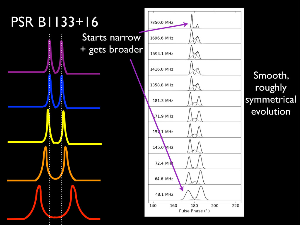
between 925 and 328 MHz (Gould & Lyne 1998; Edwards & Stappers 2003b), and LOFAR polarisation profile at 136 MHz (black lines) plotted along with the Stokes I profiles at each frequency (grey lines). The polarised com- ponent moves from the position of the leading component of the profile towards later pulse longitudes, tracing the broad component of the pulse profile. The width of the conal components as a function of fre- quency has been a subject of interest in the past. Mitra & Rankin (2002) found that the component widths remain constant be- tween 40 and 3000 MHz. We also see evidence of this in our model above 80 MHz, although the component widths begin to broaden below this value. Mitra & Rankin (2002) also no- ticed this broadening, and attributed it to dispersive smearing across a frequency channel or scattering from the ISM. In our observations, the dispersive smearing at 48 MHz (across a sin- gle 12 kHz channel) is 1.5o, which is enough to explain the observed broadening in the profile10. However, even disregard- ing this low frequency broadening Mitra & Rankin (2002) found that the spacing between the components between 100 MHz and 10 GHz changes too rapidly to be caused by a dipolar magnetic field. PSR B1133+16 is the pulsar which is most consistent with radius-to-frequency mapping of all the pulsars in our sample. However, in Section 6 we showed that its emission is confined to a very narrow region in the magnetosphere (<59 km) which is incompatible with the standard radius-to-frequency model. Radius-to-frequency mapping assumes that the emission at a given emission height traces the last open field line in the pulsar magnetosphere. From geometrical arguments (see for example Lorimer & Kramer 2005) it is possible to write the opening an- 10 The half power width of component 1 increases from 1.9o at 72 MHz to 3.6o at 48 MHz, and component 2 increases from 2.1o at 72 MHz to 3.4o at 48 MHz. Starts narrow + gets broader Smooth, roughly symmetrical evolution
between 925 and 328 MHz (Gould & Lyne 1998; Edwards & Stappers 2003b), and LOFAR polarisation profile at 136 MHz (black lines) plotted along with the Stokes I profiles at each frequency (grey lines). The polarised com- ponent moves from the position of the leading component of the profile towards later pulse longitudes, tracing the broad component of the pulse profile. The width of the conal components as a function of fre- quency has been a subject of interest in the past. Mitra & Rankin (2002) found that the component widths remain constant be- tween 40 and 3000 MHz. We also see evidence of this in our model above 80 MHz, although the component widths begin to broaden below this value. Mitra & Rankin (2002) also no- ticed this broadening, and attributed it to dispersive smearing across a frequency channel or scattering from the ISM. In our observations, the dispersive smearing at 48 MHz (across a sin- gle 12 kHz channel) is 1.5o, which is enough to explain the observed broadening in the profile10. However, even disregard- ing this low frequency broadening Mitra & Rankin (2002) found that the spacing between the components between 100 MHz and 10 GHz changes too rapidly to be caused by a dipolar magnetic field. PSR B1133+16 is the pulsar which is most consistent with radius-to-frequency mapping of all the pulsars in our sample. However, in Section 6 we showed that its emission is confined to a very narrow region in the magnetosphere (<59 km) which is incompatible with the standard radius-to-frequency model. Radius-to-frequency mapping assumes that the emission at a given emission height traces the last open field line in the pulsar magnetosphere. From geometrical arguments (see for example Lorimer & Kramer 2005) it is possible to write the opening an- 10 The half power width of component 1 increases from 1.9o at 72 MHz to 3.6o at 48 MHz, and component 2 increases from 2.1o at 72 MHz to 3.4o at 48 MHz. Starts narrow + gets broader Smooth, roughly symmetrical evolution All pulses arrive at the same time
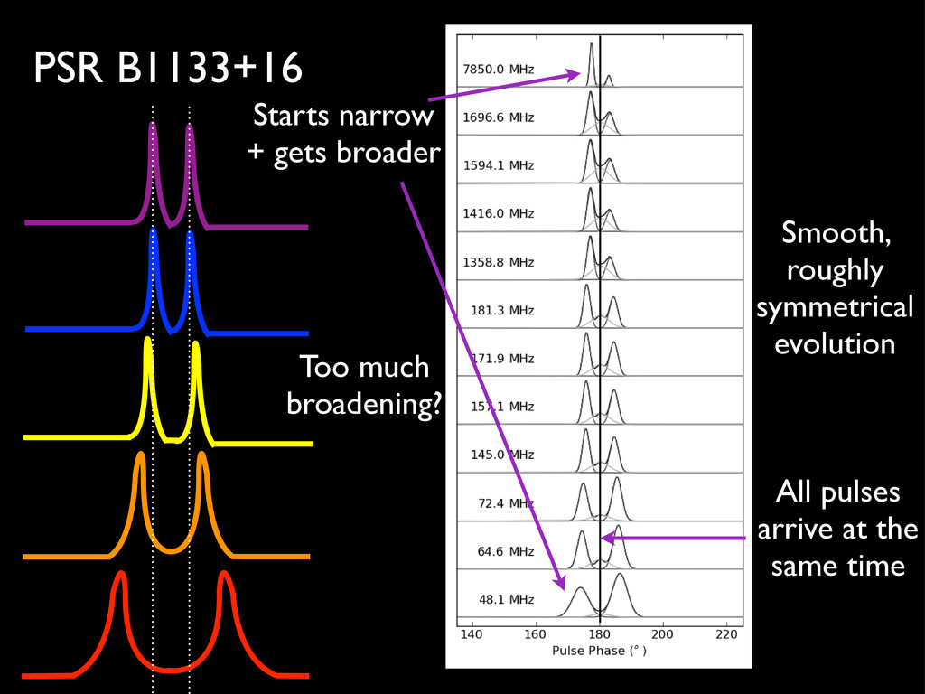
between 925 and 328 MHz (Gould & Lyne 1998; Edwards & Stappers 2003b), and LOFAR polarisation profile at 136 MHz (black lines) plotted along with the Stokes I profiles at each frequency (grey lines). The polarised com- ponent moves from the position of the leading component of the profile towards later pulse longitudes, tracing the broad component of the pulse profile. The width of the conal components as a function of fre- quency has been a subject of interest in the past. Mitra & Rankin (2002) found that the component widths remain constant be- tween 40 and 3000 MHz. We also see evidence of this in our model above 80 MHz, although the component widths begin to broaden below this value. Mitra & Rankin (2002) also no- ticed this broadening, and attributed it to dispersive smearing across a frequency channel or scattering from the ISM. In our observations, the dispersive smearing at 48 MHz (across a sin- gle 12 kHz channel) is 1.5o, which is enough to explain the observed broadening in the profile10. However, even disregard- ing this low frequency broadening Mitra & Rankin (2002) found that the spacing between the components between 100 MHz and 10 GHz changes too rapidly to be caused by a dipolar magnetic field. PSR B1133+16 is the pulsar which is most consistent with radius-to-frequency mapping of all the pulsars in our sample. However, in Section 6 we showed that its emission is confined to a very narrow region in the magnetosphere (<59 km) which is incompatible with the standard radius-to-frequency model. Radius-to-frequency mapping assumes that the emission at a given emission height traces the last open field line in the pulsar magnetosphere. From geometrical arguments (see for example Lorimer & Kramer 2005) it is possible to write the opening an- 10 The half power width of component 1 increases from 1.9o at 72 MHz to 3.6o at 48 MHz, and component 2 increases from 2.1o at 72 MHz to 3.4o at 48 MHz. Starts narrow + gets broader Smooth, roughly symmetrical evolution All pulses arrive at the same time Too much broadening?
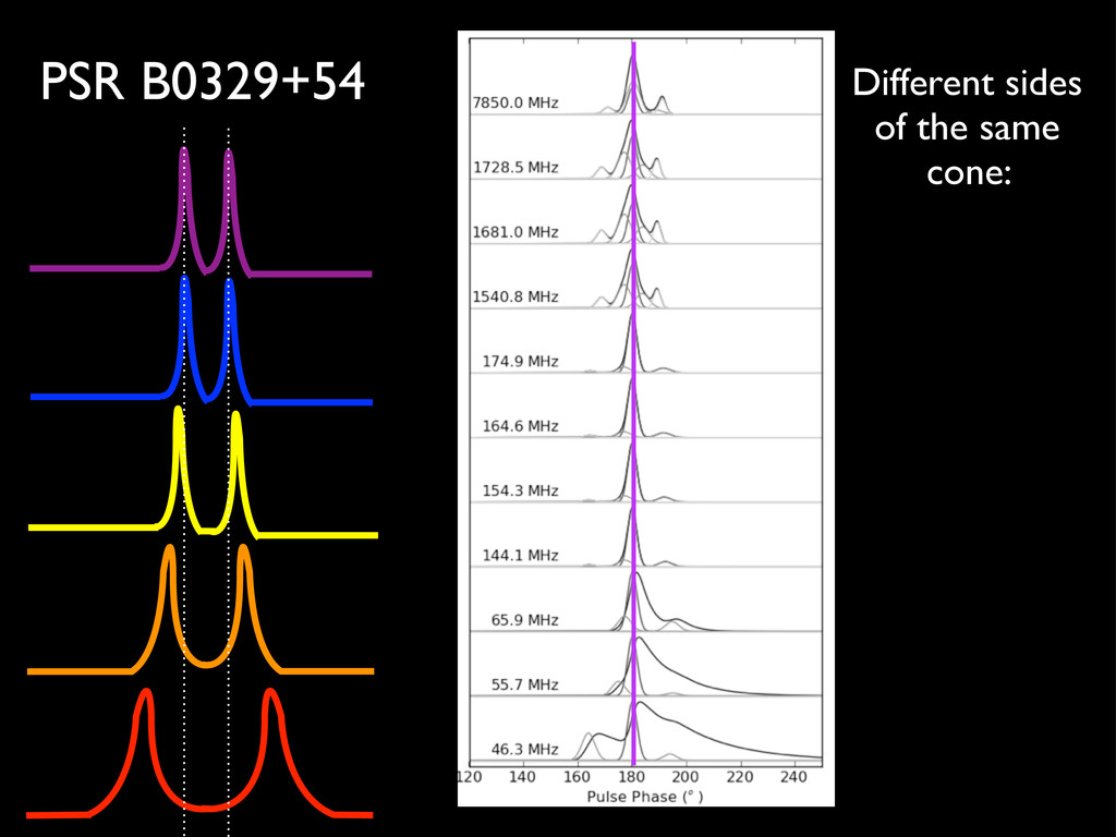
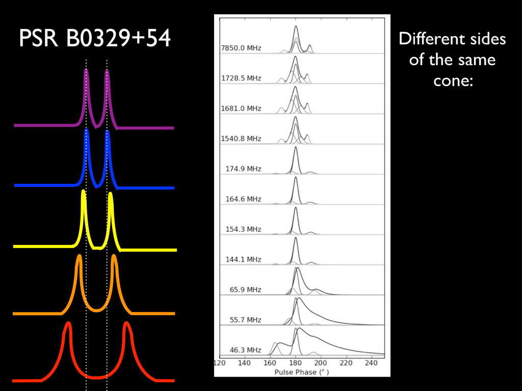
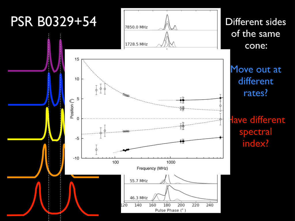
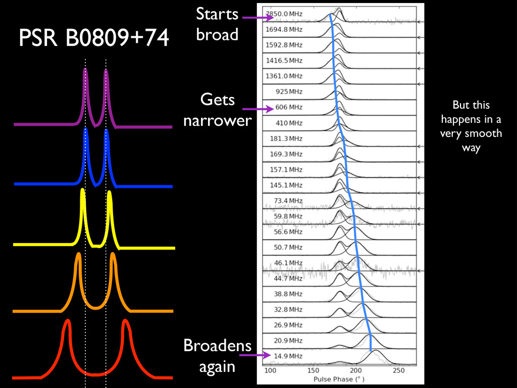
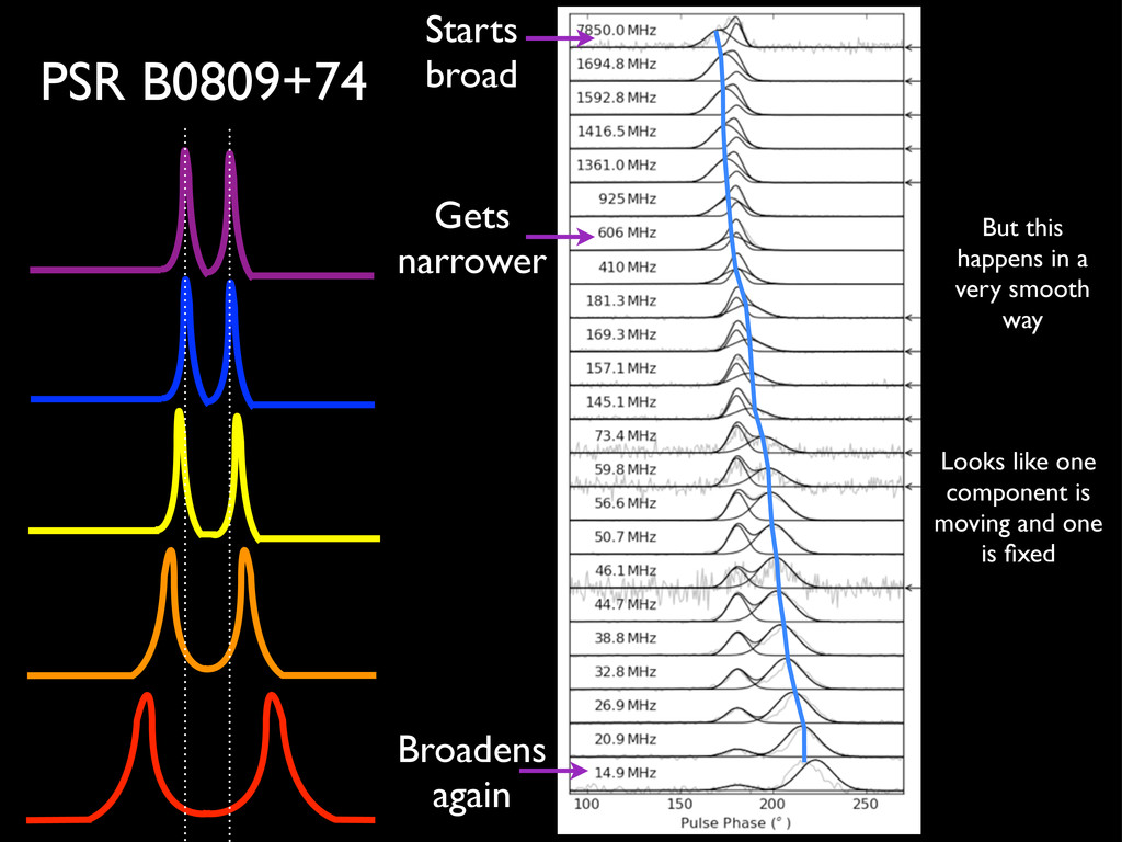
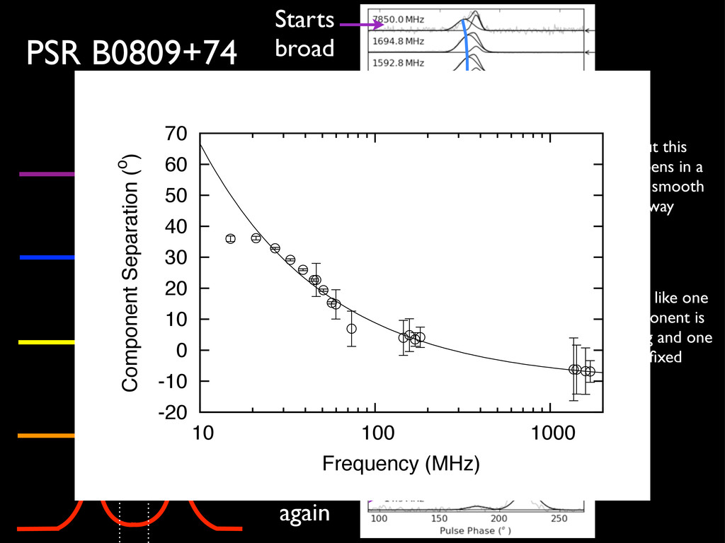
happens in a very smooth way Looks like one component is moving and one is fixed -20 -10 0 10 20 30 40 50 60 70 10 100 1000 Component Separation (o) Frequency (MHz)
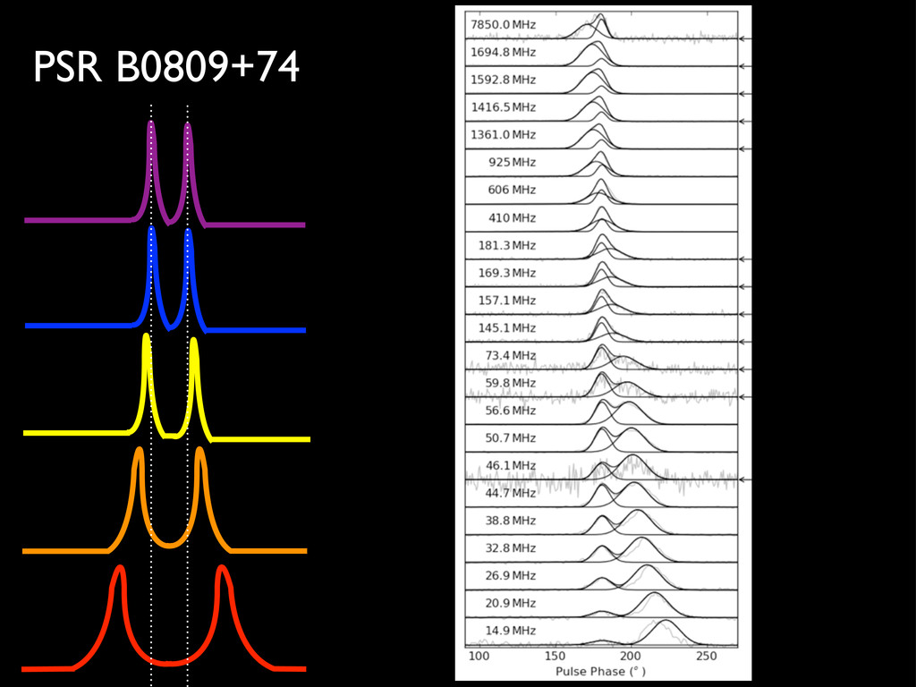
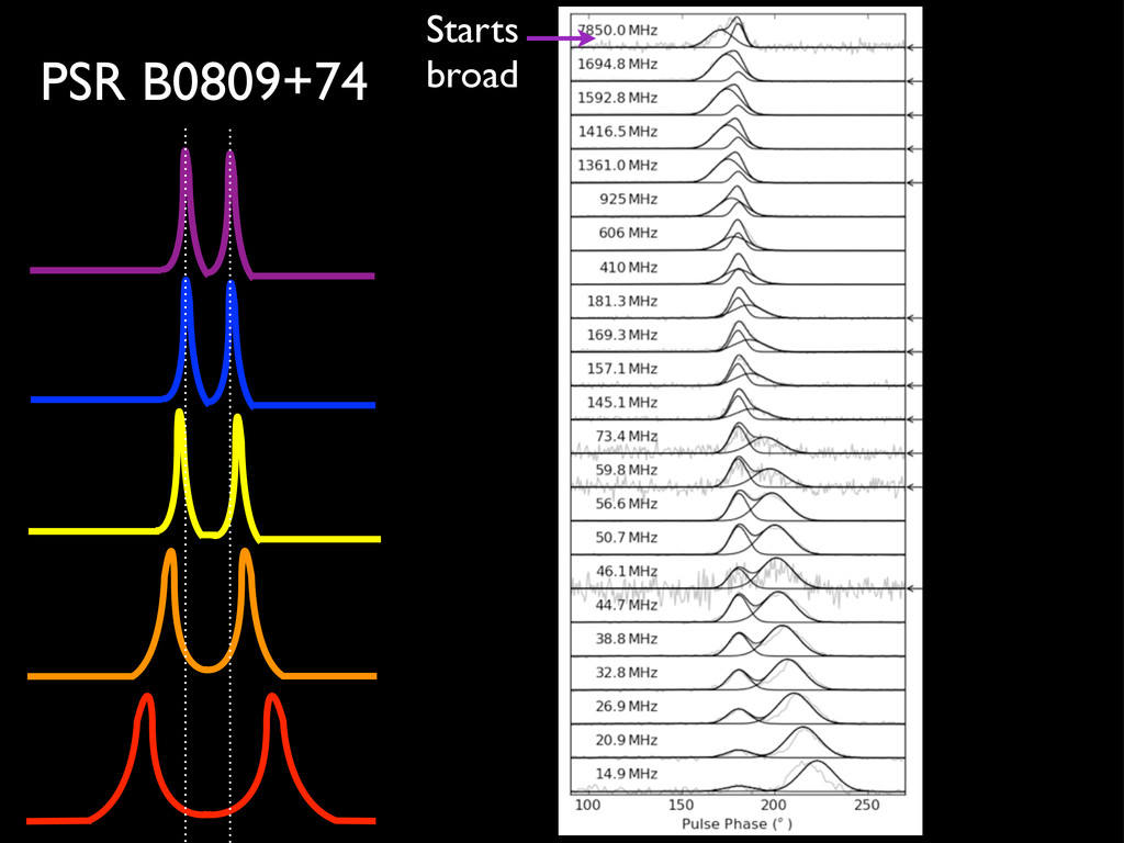
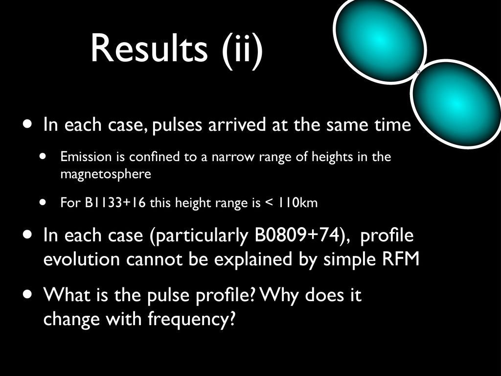
same time • Emission is confined to a narrow range of heights in the magnetosphere • For B1133+16 this height range is < 110km • In each case (particularly B0809+74), profile evolution cannot be explained by simple RFM • What is the pulse profile? Why does it change with frequency?
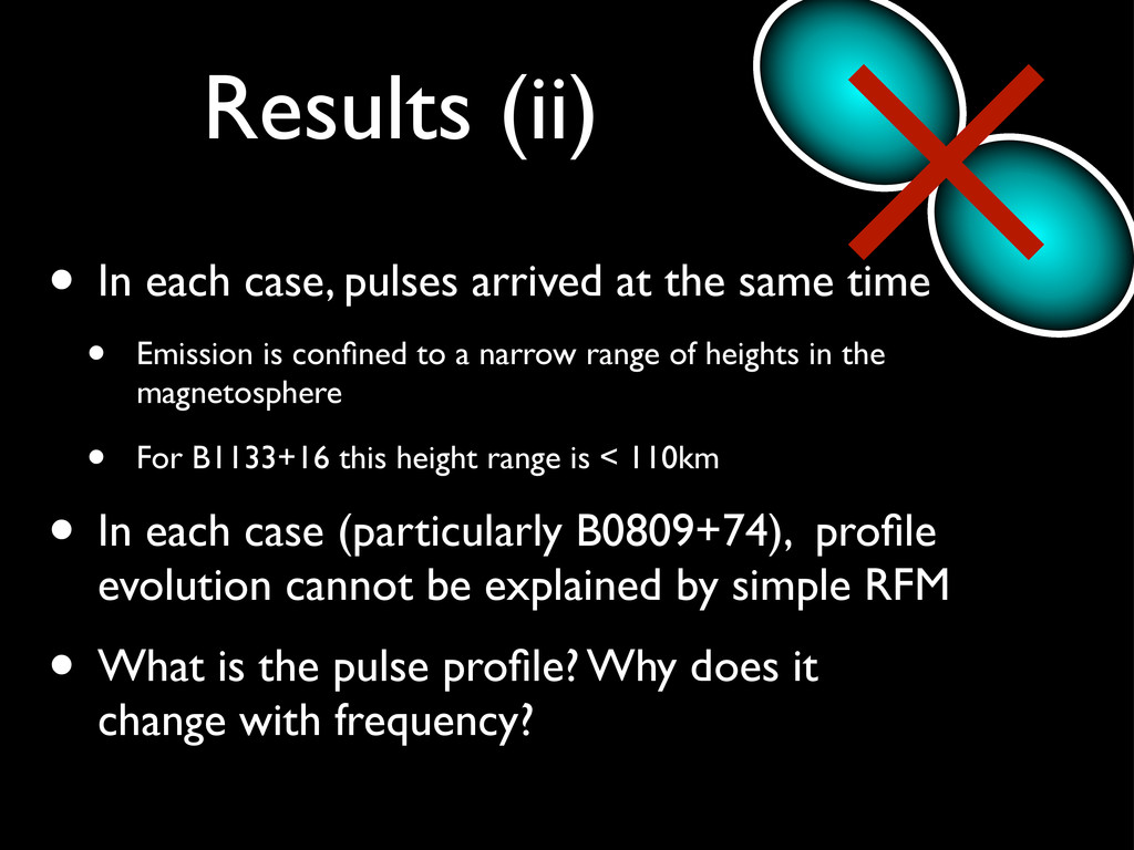
same time • Emission is confined to a narrow range of heights in the magnetosphere • For B1133+16 this height range is < 110km • In each case (particularly B0809+74), profile evolution cannot be explained by simple RFM • What is the pulse profile? Why does it change with frequency?
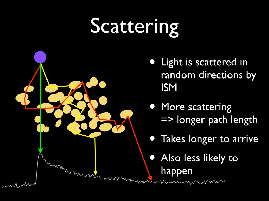
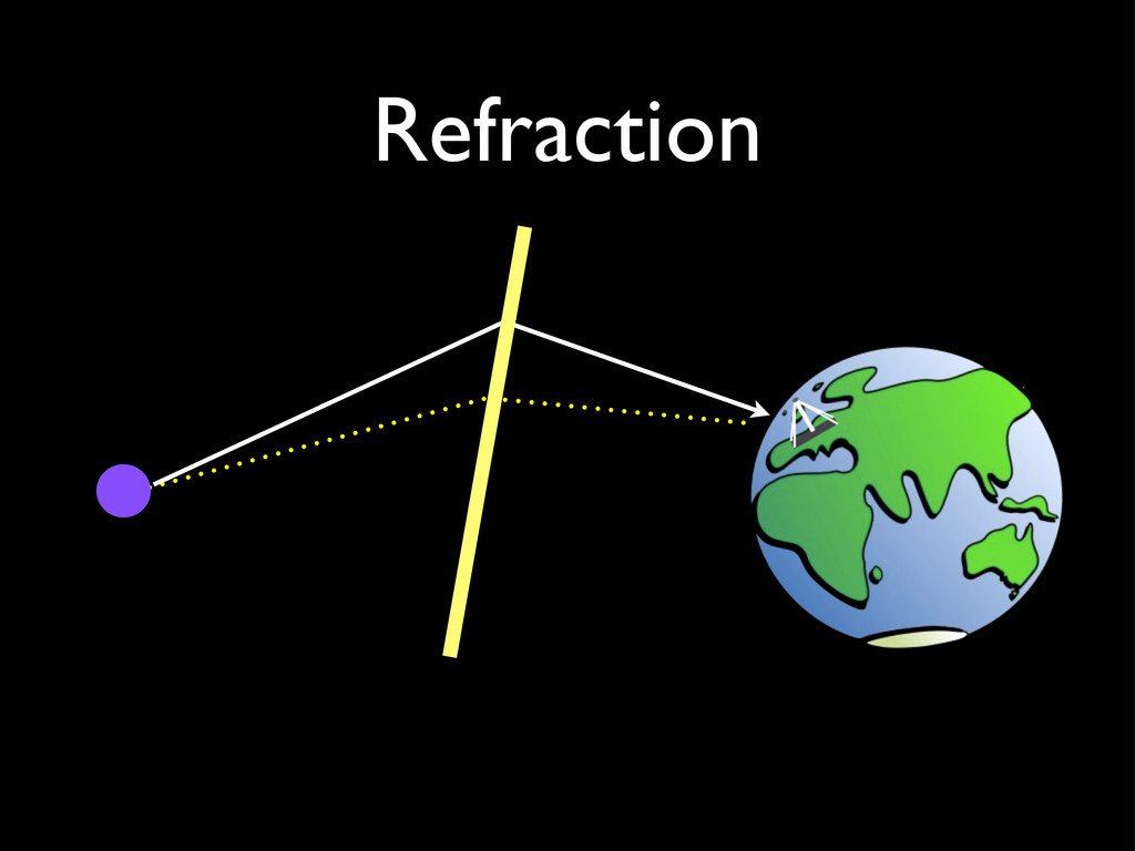
through the magnetosphere • Emission all comes from a narrow height range and propagation effects cause the profile to change shape (Beskin & Philippov 2011) • E.g. For B0809+74: One component is refracted, and one is not If not RFM, then what?