Jumps and Proper Forward Rate Curves The Case of Synthetic Deposits in Legacy Discount-Based Systems Ferdinando M. Ametrano [email protected] Paolo Mazzocchi [email protected] QuantLib User Meeting 2014 5 December 2014 Ferdinando M. Ametrano, Paolo Mazzocchi QuantLib User Meeting 2014 1 / 66
1 Synthetic Deposits The problem A first solution Residual problems 2 ON Curve with Jumps Jumps detection Jumps calculation 3 Final Results Forward rate curve using Synthetic Deposits Ferdinando M. Ametrano, Paolo Mazzocchi QuantLib User Meeting 2014 2 / 66
1 Synthetic Deposits The problem A first solution Residual problems 2 ON Curve with Jumps Jumps detection Jumps calculation 3 Final Results Forward rate curve using Synthetic Deposits Ferdinando M. Ametrano, Paolo Mazzocchi QuantLib User Meeting 2014 3 / 66
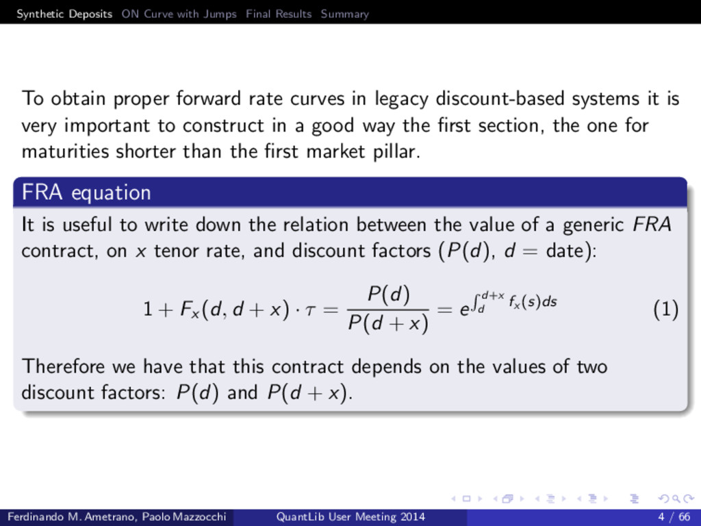
obtain proper forward rate curves in legacy discount-based systems it is very important to construct in a good way the first section, the one for maturities shorter than the first market pillar. FRA equation It is useful to write down the relation between the value of a generic FRA contract, on x tenor rate, and discount factors (P(d), d = date): 1 + Fx (d, d + x) · τ = P(d) P(d + x) = e d+x d fx (s)ds (1) Therefore we have that this contract depends on the values of two discount factors: P(d) and P(d + x). Ferdinando M. Ametrano, Paolo Mazzocchi QuantLib User Meeting 2014 4 / 66
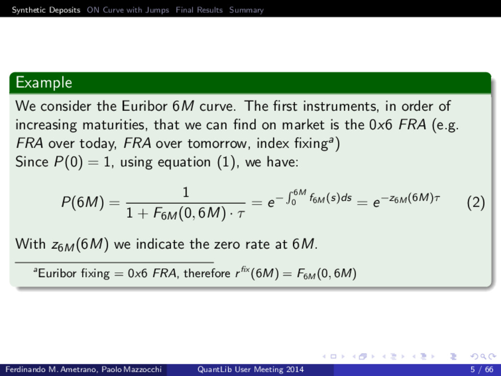
We consider the Euribor 6M curve. The first instruments, in order of increasing maturities, that we can find on market is the 0x6 FRA (e.g. FRA over today, FRA over tomorrow, index fixinga) Since P(0) = 1, using equation (1), we have: P(6M) = 1 1 + F6M(0, 6M) · τ = e− 6M 0 f6M (s)ds = e−z6M (6M)τ (2) With z6M(6M) we indicate the zero rate at 6M. aEuribor fixing = 0x6 FRA, therefore rfix (6M) = F6M (0, 6M) Ferdinando M. Ametrano, Paolo Mazzocchi QuantLib User Meeting 2014 5 / 66
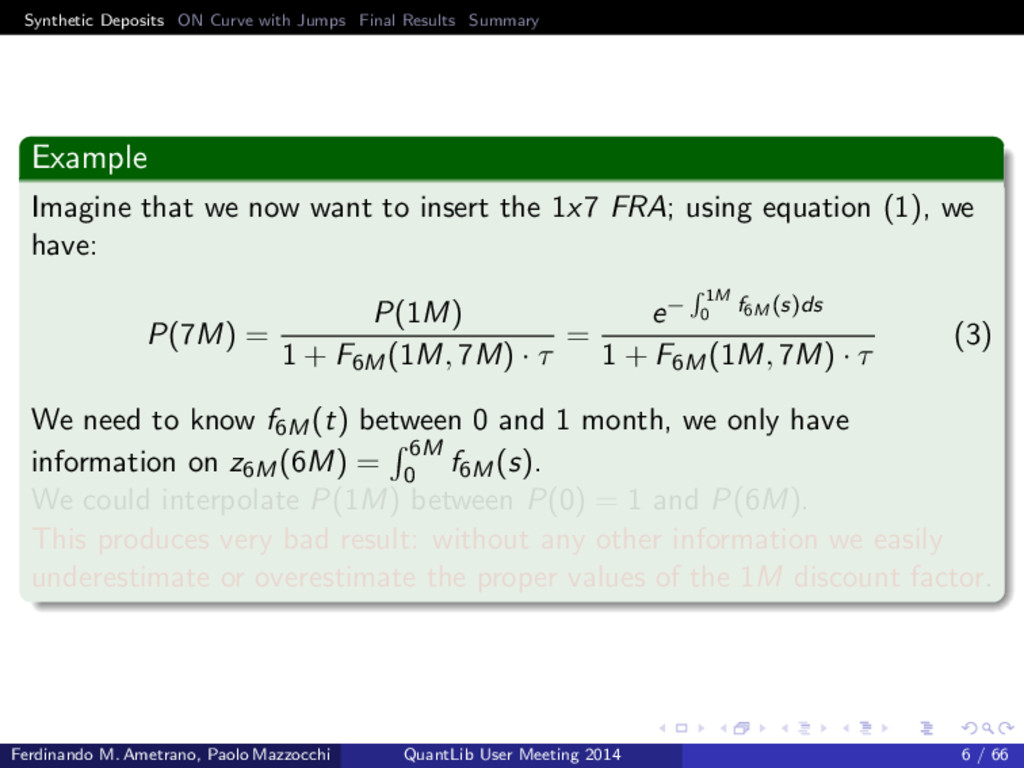
Imagine that we now want to insert the 1x7 FRA; using equation (1), we have: P(7M) = P(1M) 1 + F6M(1M, 7M) · τ = e− 1M 0 f6M (s)ds 1 + F6M(1M, 7M) · τ (3) We need to know f6M(t) between 0 and 1 month, we only have information on z6M(6M) = 6M 0 f6M(s). We could interpolate P(1M) between P(0) = 1 and P(6M). This produces very bad result: without any other information we easily underestimate or overestimate the proper values of the 1M discount factor. Ferdinando M. Ametrano, Paolo Mazzocchi QuantLib User Meeting 2014 6 / 66
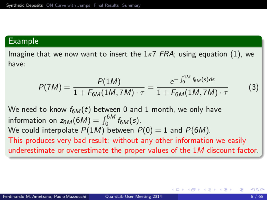
Imagine that we now want to insert the 1x7 FRA; using equation (1), we have: P(7M) = P(1M) 1 + F6M(1M, 7M) · τ = e− 1M 0 f6M (s)ds 1 + F6M(1M, 7M) · τ (3) We need to know f6M(t) between 0 and 1 month, we only have information on z6M(6M) = 6M 0 f6M(s). We could interpolate P(1M) between P(0) = 1 and P(6M). This produces very bad result: without any other information we easily underestimate or overestimate the proper values of the 1M discount factor. Ferdinando M. Ametrano, Paolo Mazzocchi QuantLib User Meeting 2014 6 / 66
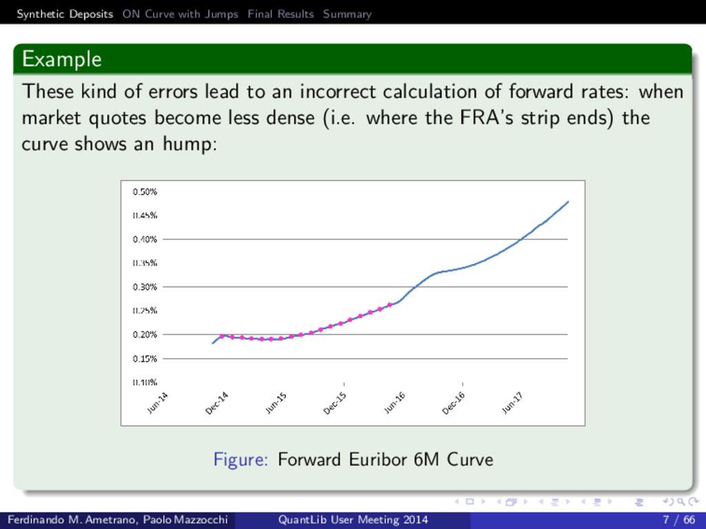
These kind of errors lead to an incorrect calculation of forward rates: when market quotes become less dense (i.e. where the FRA’s strip ends) the curve shows an hump: Figure: Forward Euribor 6M Curve Ferdinando M. Ametrano, Paolo Mazzocchi QuantLib User Meeting 2014 7 / 66
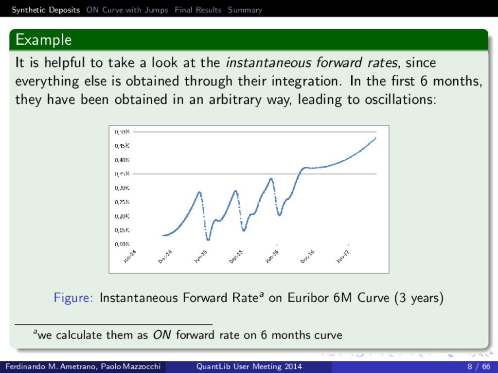
It is helpful to take a look at the instantaneous forward rates, since everything else is obtained through their integration. In the first 6 months, they have been obtained in an arbitrary way, leading to oscillations: Figure: Instantaneous Forward Ratea on Euribor 6M Curve (3 years) awe calculate them as ON forward rate on 6 months curve Ferdinando M. Ametrano, Paolo Mazzocchi QuantLib User Meeting 2014 8 / 66
1 Synthetic Deposits The problem A first solution Residual problems 2 ON Curve with Jumps Jumps detection Jumps calculation 3 Final Results Forward rate curve using Synthetic Deposits Ferdinando M. Ametrano, Paolo Mazzocchi QuantLib User Meeting 2014 9 / 66
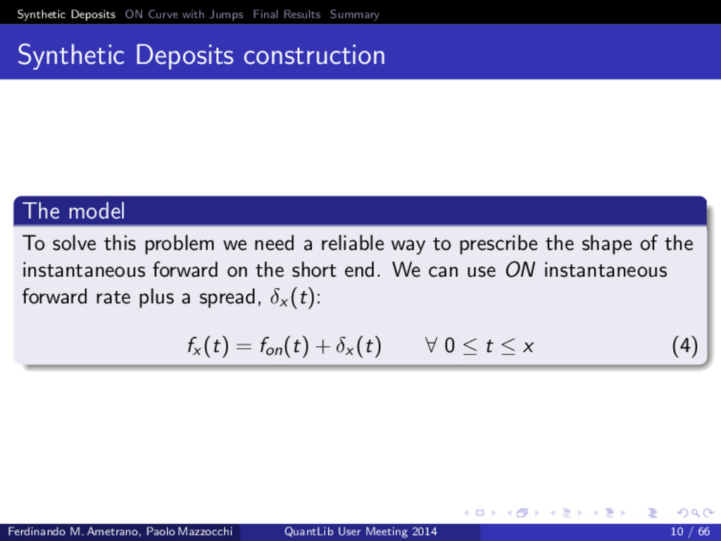
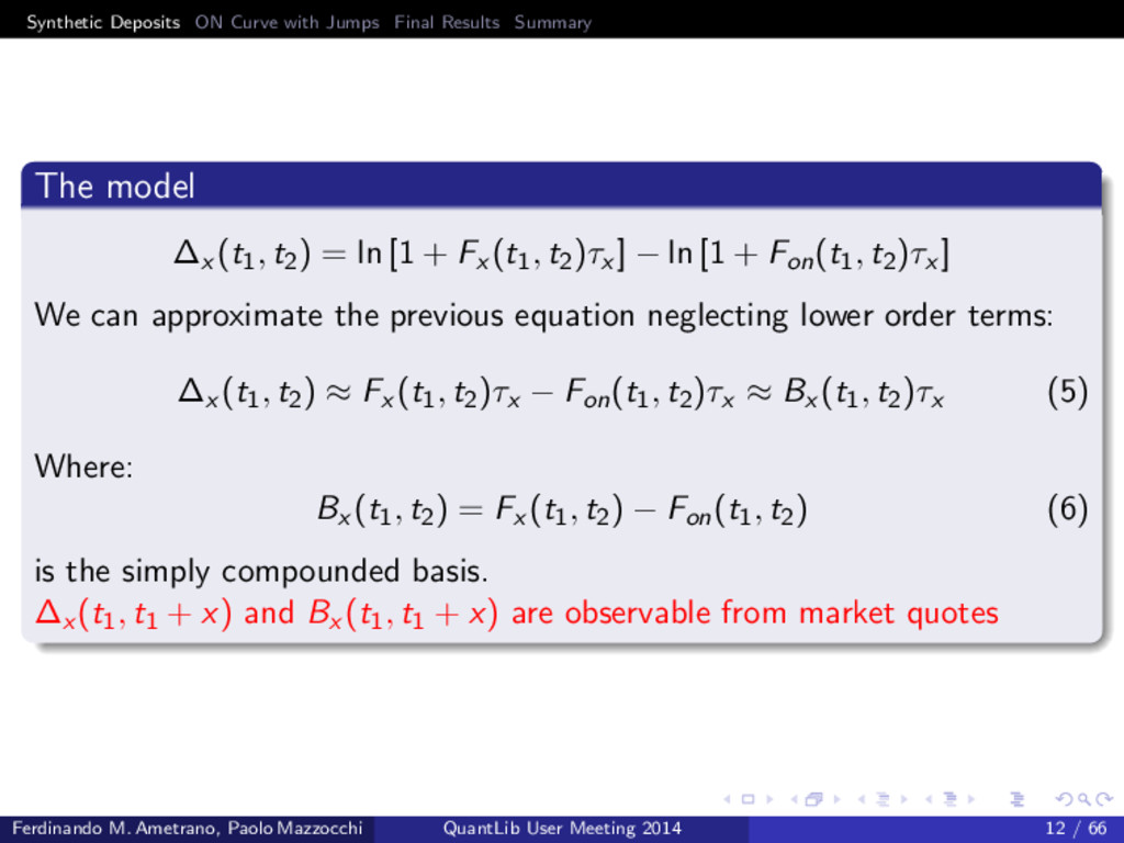
Deposits construction The model To solve this problem we need a reliable way to prescribe the shape of the instantaneous forward on the short end. We can use ON instantaneous forward rate plus a spread, δx (t): fx (t) = fon(t) + δx (t) ∀ 0 ≤ t ≤ x (4) Ferdinando M. Ametrano, Paolo Mazzocchi QuantLib User Meeting 2014 10 / 66
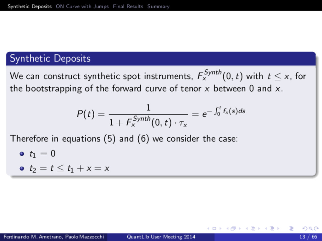
Deposits We can construct synthetic spot instruments, FSynth x (0, t) with t ≤ x, for the bootstrapping of the forward curve of tenor x between 0 and x. P(t) = 1 1 + FSynth x (0, t) · τx = e− t 0 fx (s)ds Therefore in equations (5) and (6) we consider the case: t1 = 0 t2 = t ≤ t1 + x = x Ferdinando M. Ametrano, Paolo Mazzocchi QuantLib User Meeting 2014 13 / 66
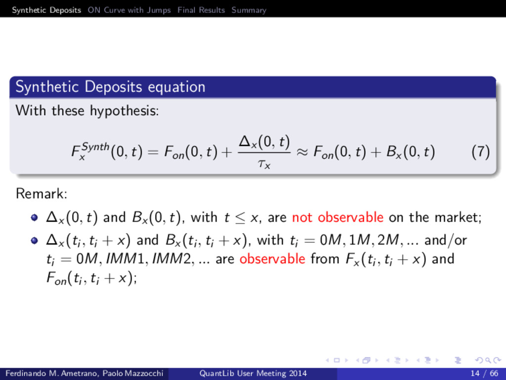
Deposits equation With these hypothesis: FSynth x (0, t) = Fon(0, t) + ∆x (0, t) τx ≈ Fon(0, t) + Bx (0, t) (7) Remark: ∆x (0, t) and Bx (0, t), with t ≤ x, are not observable on the market; ∆x (ti , ti + x) and Bx (ti , ti + x), with ti = 0M, 1M, 2M, ... and/or ti = 0M, IMM1, IMM2, ... are observable from Fx (ti , ti + x) and Fon(ti , ti + x); Ferdinando M. Ametrano, Paolo Mazzocchi QuantLib User Meeting 2014 14 / 66
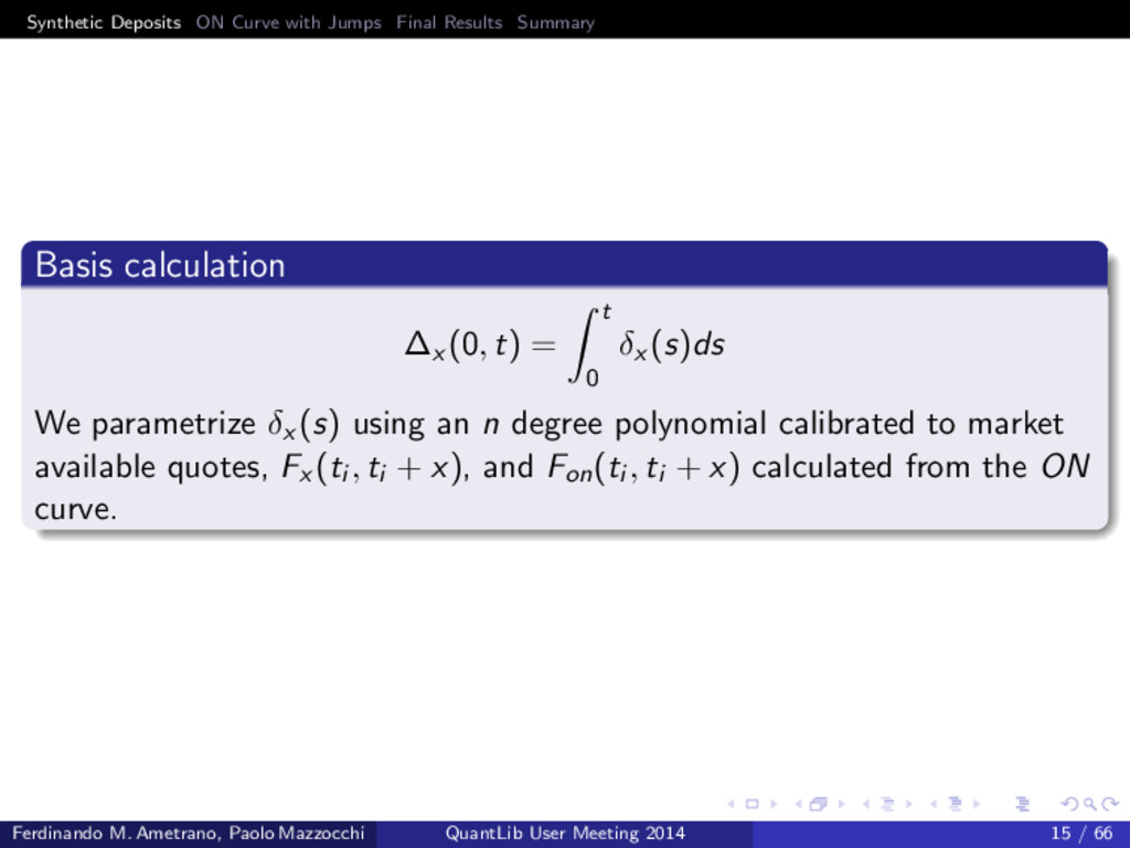
calculation ∆x (0, t) = t 0 δx (s)ds We parametrize δx (s) using an n degree polynomial calibrated to market available quotes, Fx (ti , ti + x), and Fon(ti , ti + x) calculated from the ON curve. Ferdinando M. Ametrano, Paolo Mazzocchi QuantLib User Meeting 2014 15 / 66
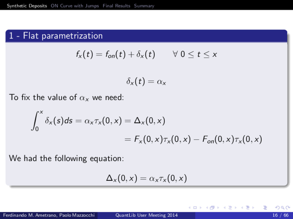
- Flat parametrization fx (t) = fon(t) + δx (t) ∀ 0 ≤ t ≤ x δx (t) = αx To fix the value of αx we need: x 0 δx (s)ds = αx τx (0, x) = ∆x (0, x) = Fx (0, x)τx (0, x) − Fon(0, x)τx (0, x) We had the following equation: ∆x (0, x) = αx τx (0, x) Ferdinando M. Ametrano, Paolo Mazzocchi QuantLib User Meeting 2014 16 / 66
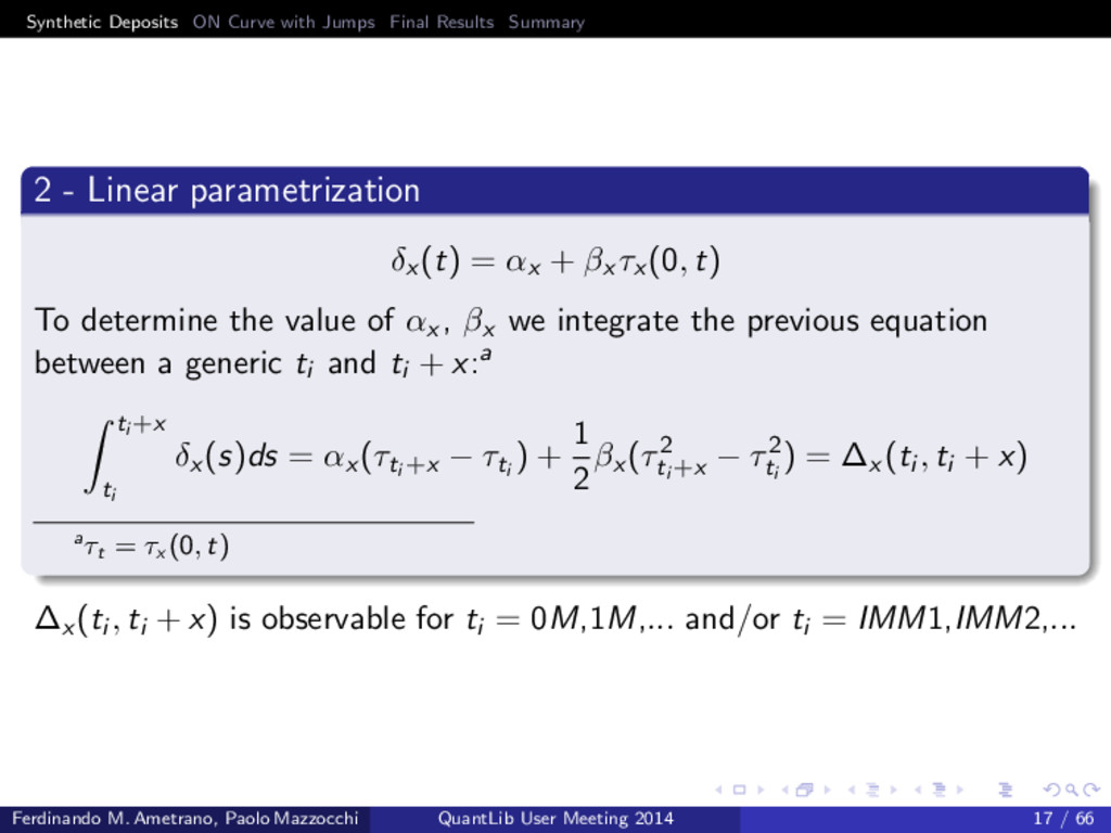
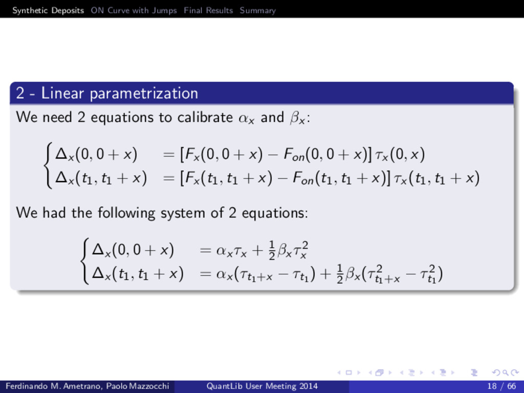
- Linear parametrization δx (t) = αx + βx τx (0, t) To determine the value of αx , βx we integrate the previous equation between a generic ti and ti + x:a ti +x ti δx (s)ds = αx (τti +x − τti ) + 1 2 βx (τ2 ti +x − τ2 ti ) = ∆x (ti , ti + x) aτt = τx (0, t) ∆x (ti , ti + x) is observable for ti = 0M,1M,... and/or ti = IMM1,IMM2,... Ferdinando M. Ametrano, Paolo Mazzocchi QuantLib User Meeting 2014 17 / 66
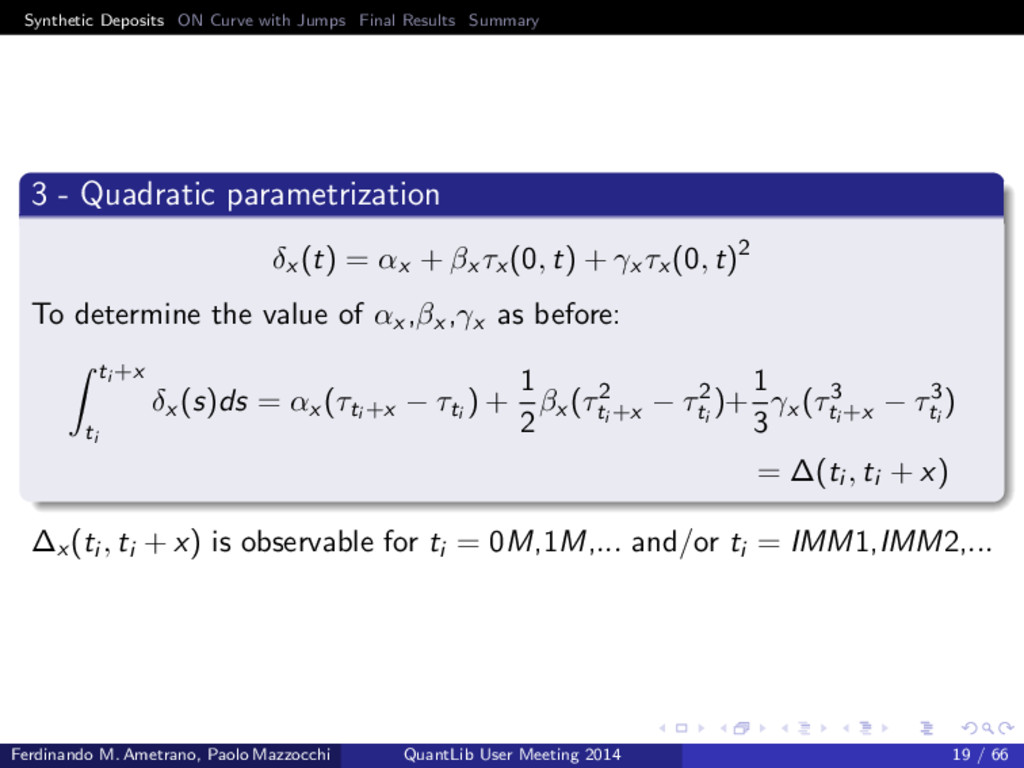
- Quadratic parametrization δx (t) = αx + βx τx (0, t) + γx τx (0, t)2 To determine the value of αx ,βx ,γx as before: ti +x ti δx (s)ds = αx (τti +x − τti ) + 1 2 βx (τ2 ti +x − τ2 ti )+ 1 3 γx (τ3 ti +x − τ3 ti ) = ∆(ti , ti + x) ∆x (ti , ti + x) is observable for ti = 0M,1M,... and/or ti = IMM1,IMM2,... Ferdinando M. Ametrano, Paolo Mazzocchi QuantLib User Meeting 2014 19 / 66
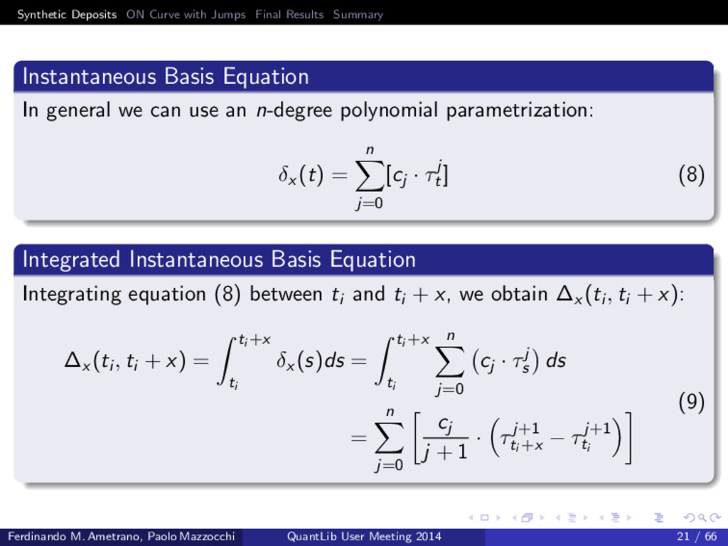
Basis Equation In general we can use an n-degree polynomial parametrization: δx (t) = n j=0 [cj · τj t ] (8) Integrated Instantaneous Basis Equation Integrating equation (8) between ti and ti + x, we obtain ∆x (ti , ti + x): ∆x (ti , ti + x) = ti +x ti δx (s)ds = ti +x ti n j=0 cj · τj s ds = n j=0 cj j + 1 · τj+1 ti +x − τj+1 ti (9) Ferdinando M. Ametrano, Paolo Mazzocchi QuantLib User Meeting 2014 21 / 66
find ∆x (ti , ti + x) we use: market available quotes on x-months tenor Euribor/Libor, like: index fixing, Futures, FRA, IRS. equivalent ON discrete forward rates, built using the ON curve (in the Euro market they are equivalent to forward OIS contract). Ferdinando M. Ametrano, Paolo Mazzocchi QuantLib User Meeting 2014 22 / 66
Calculation Example Let’s consider the 6 Months Euribor curve. Until 2 years ago, to calculate ∆6M(0, 6M) we had: FRA over today and FRA over tomorrow; Today they are not quoted anymore, therefore we need to find a different way to calculate ∆6M(0, 6M). The only contract that we can use is the index fixing. After that instruments, to calculate ∆6M(ti , ti + x), we have: FRA up to 2 years. We calculate ON discrete forward rates insisting on the same set of dates as the 6M market quotes and we calculate the difference between these two values. Ferdinando M. Ametrano, Paolo Mazzocchi QuantLib User Meeting 2014 23 / 66
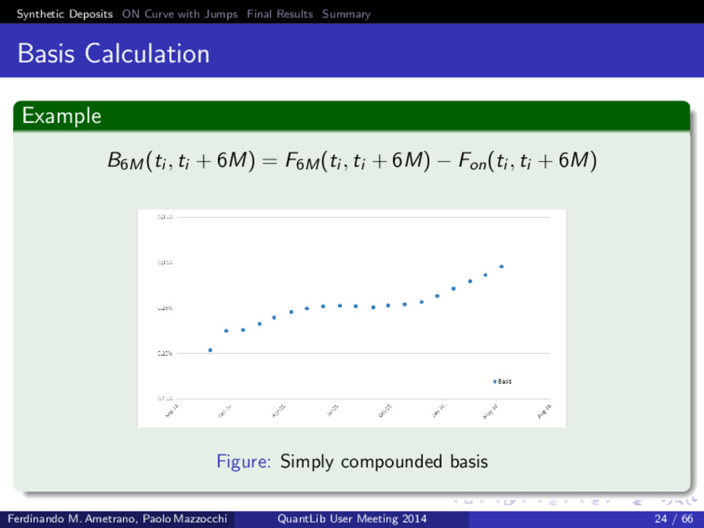
Calculation Example B6M(ti , ti + 6M) = F6M(ti , ti + 6M) − Fon(ti , ti + 6M) Figure: Simply compounded basis Ferdinando M. Ametrano, Paolo Mazzocchi QuantLib User Meeting 2014 24 / 66
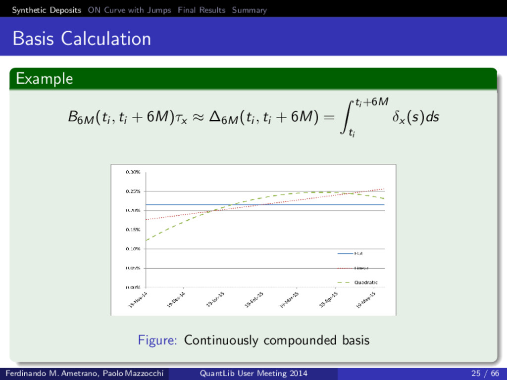
Calculation Example B6M(ti , ti + 6M)τx ≈ ∆6M(ti , ti + 6M) = ti +6M ti δx (s)ds Figure: Continuously compounded basis Ferdinando M. Ametrano, Paolo Mazzocchi QuantLib User Meeting 2014 25 / 66
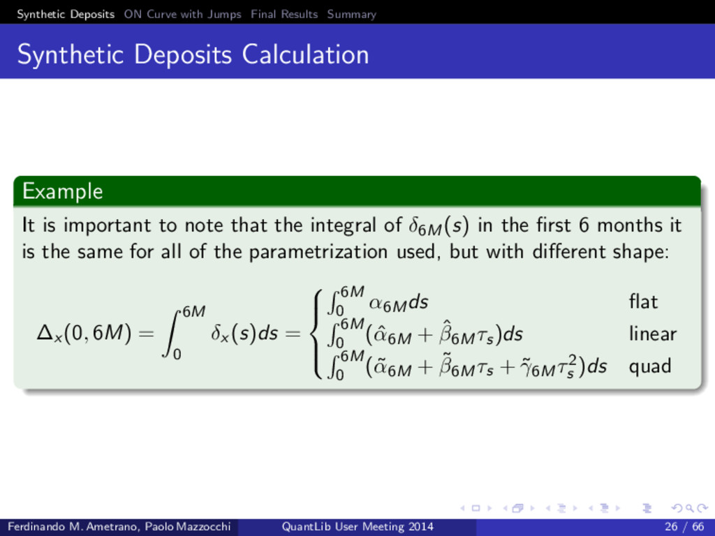
Deposits Calculation Example It is important to note that the integral of δ6M(s) in the first 6 months it is the same for all of the parametrization used, but with different shape: ∆x (0, 6M) = 6M 0 δx (s)ds = 6M 0 α6Mds flat 6M 0 (ˆ α6M + ˆ β6Mτs)ds linear 6M 0 (˜ α6M + ˜ β6Mτs + ˜ γ6Mτ2 s )ds quad Ferdinando M. Ametrano, Paolo Mazzocchi QuantLib User Meeting 2014 26 / 66
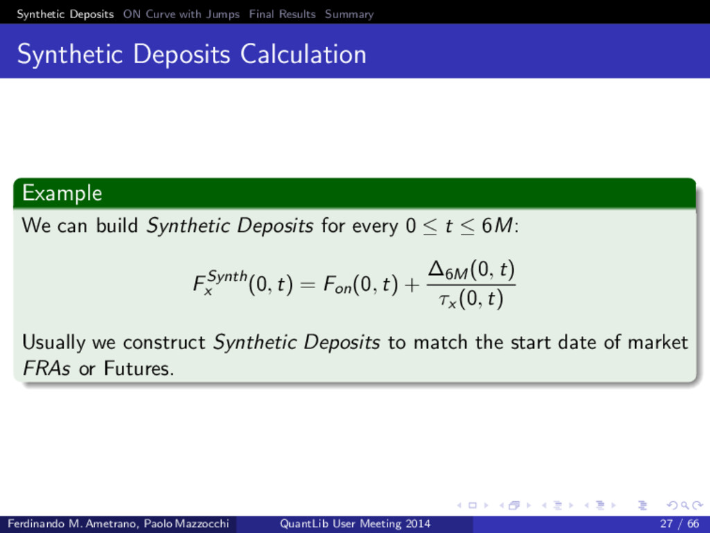
Deposits Calculation Example We can build Synthetic Deposits for every 0 ≤ t ≤ 6M: FSynth x (0, t) = Fon(0, t) + ∆6M(0, t) τx (0, t) Usually we construct Synthetic Deposits to match the start date of market FRAs or Futures. Ferdinando M. Ametrano, Paolo Mazzocchi QuantLib User Meeting 2014 27 / 66
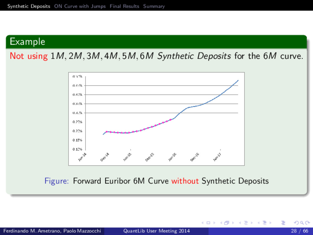
Not using 1M, 2M, 3M, 4M, 5M, 6M Synthetic Deposits for the 6M curve. Figure: Forward Euribor 6M Curve without Synthetic Deposits Ferdinando M. Ametrano, Paolo Mazzocchi QuantLib User Meeting 2014 28 / 66
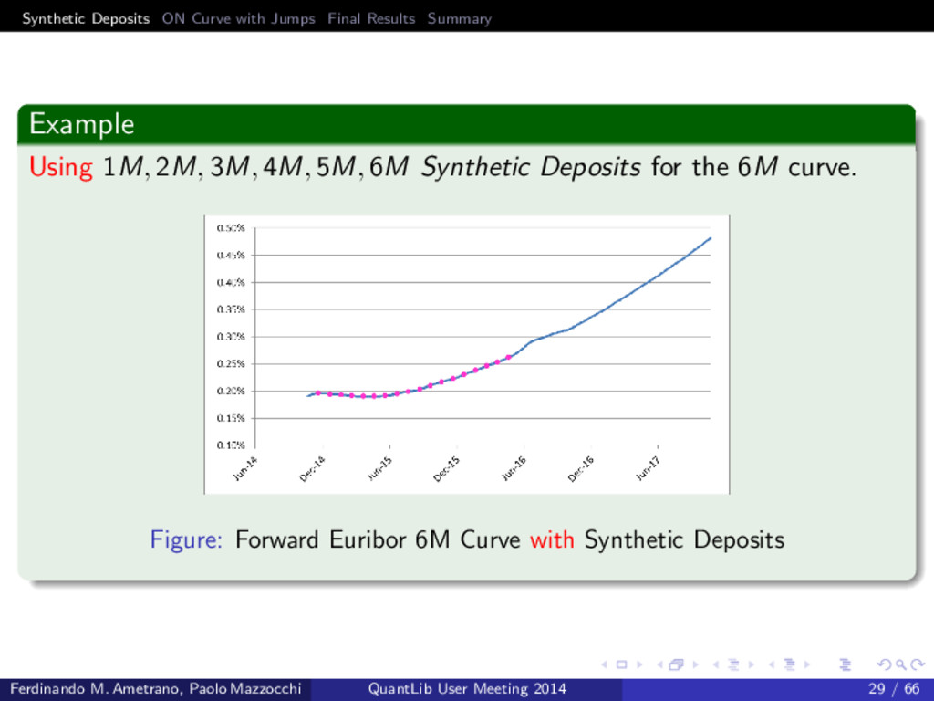
Using 1M, 2M, 3M, 4M, 5M, 6M Synthetic Deposits for the 6M curve. Figure: Forward Euribor 6M Curve with Synthetic Deposits Ferdinando M. Ametrano, Paolo Mazzocchi QuantLib User Meeting 2014 29 / 66
1 Synthetic Deposits The problem A first solution Residual problems 2 ON Curve with Jumps Jumps detection Jumps calculation 3 Final Results Forward rate curve using Synthetic Deposits Ferdinando M. Ametrano, Paolo Mazzocchi QuantLib User Meeting 2014 30 / 66
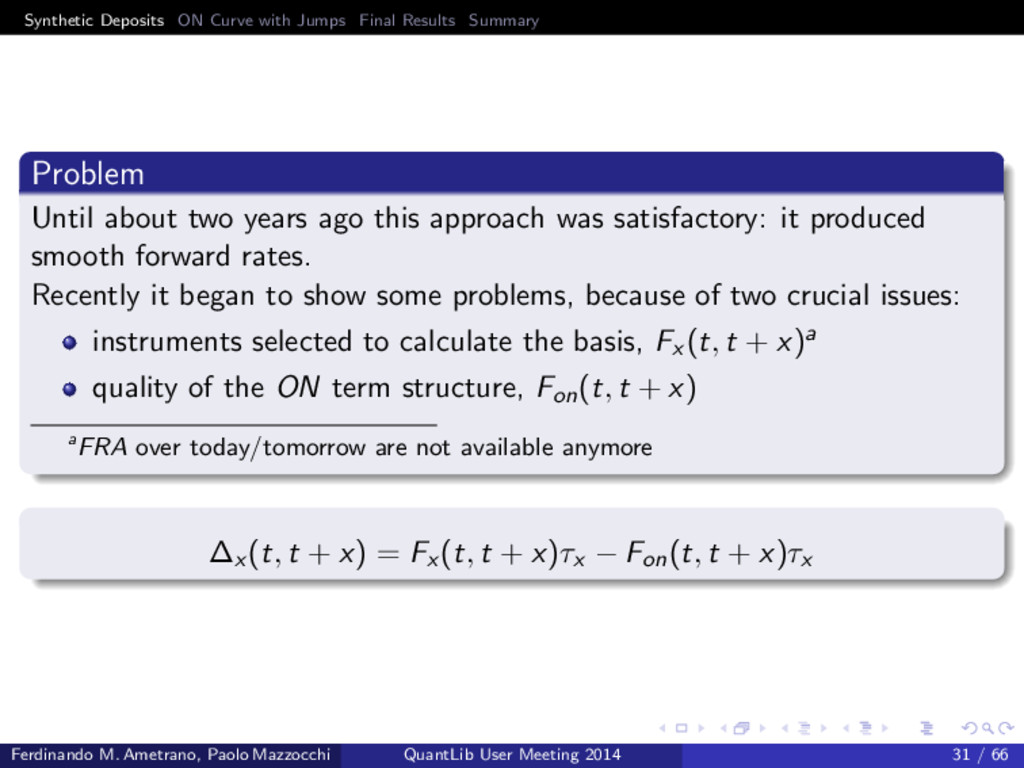
Until about two years ago this approach was satisfactory: it produced smooth forward rates. Recently it began to show some problems, because of two crucial issues: instruments selected to calculate the basis, Fx (t, t + x)a quality of the ON term structure, Fon(t, t + x) aFRA over today/tomorrow are not available anymore ∆x (t, t + x) = Fx (t, t + x)τx − Fon(t, t + x)τx Ferdinando M. Ametrano, Paolo Mazzocchi QuantLib User Meeting 2014 31 / 66
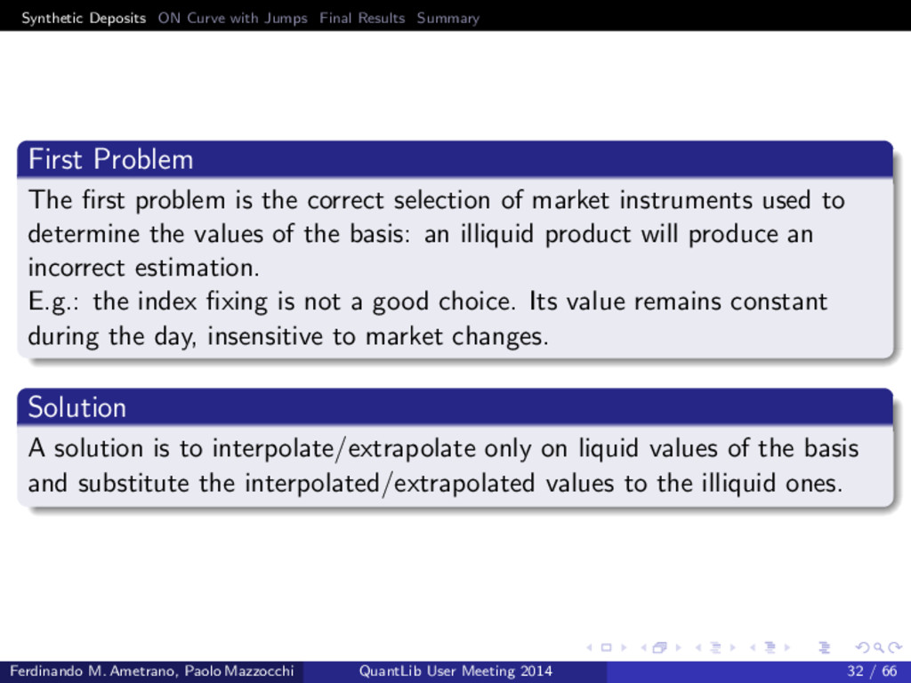
Problem The first problem is the correct selection of market instruments used to determine the values of the basis: an illiquid product will produce an incorrect estimation. E.g.: the index fixing is not a good choice. Its value remains constant during the day, insensitive to market changes. Solution A solution is to interpolate/extrapolate only on liquid values of the basis and substitute the interpolated/extrapolated values to the illiquid ones. Ferdinando M. Ametrano, Paolo Mazzocchi QuantLib User Meeting 2014 32 / 66
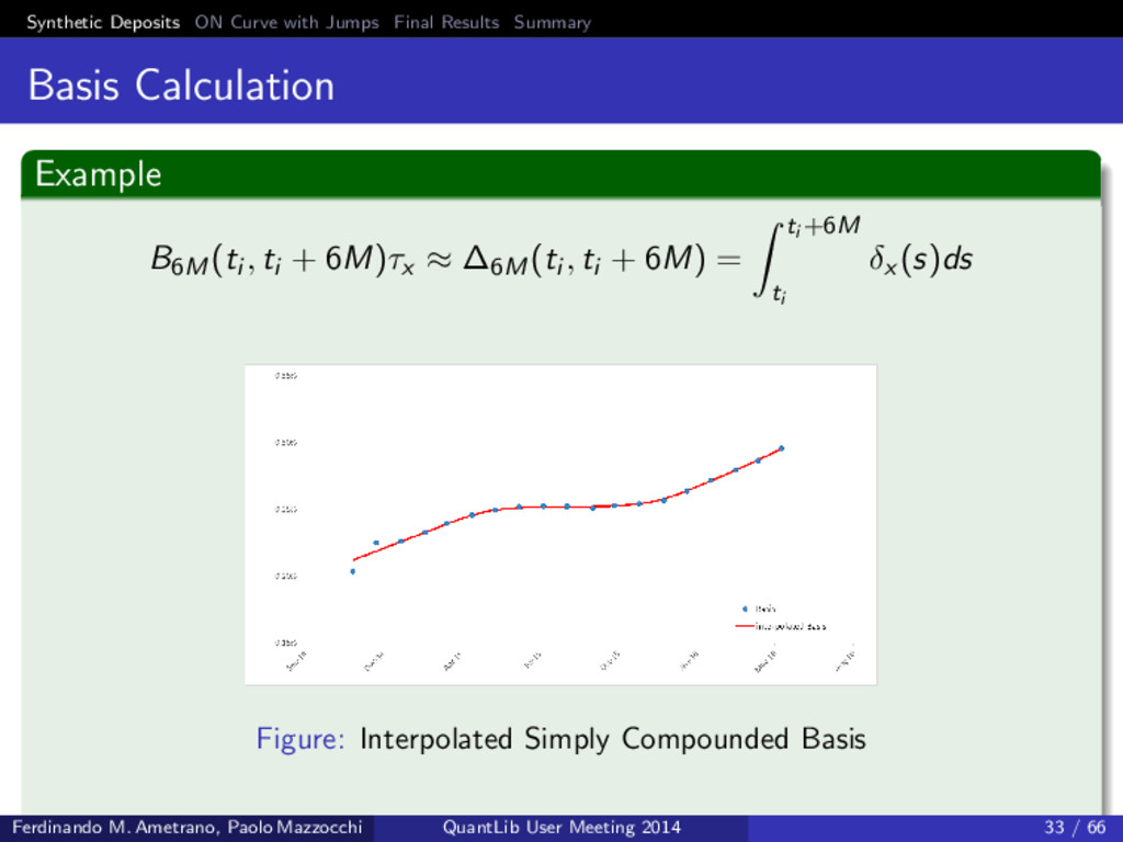
Calculation Example B6M(ti , ti + 6M)τx ≈ ∆6M(ti , ti + 6M) = ti +6M ti δx (s)ds Figure: Interpolated Simply Compounded Basis Ferdinando M. Ametrano, Paolo Mazzocchi QuantLib User Meeting 2014 33 / 66
Calculation Example B6M(ti , ti + 6M)τx ≈ ∆6M(ti , ti + 6M) = ti +6M ti δx (s)ds Figure: Interpolated Simply Compounded Basis Ferdinando M. Ametrano, Paolo Mazzocchi QuantLib User Meeting 2014 33 / 66
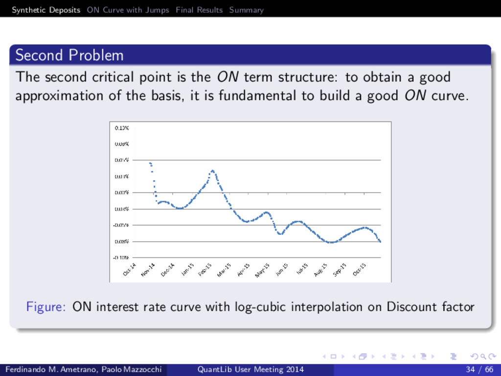
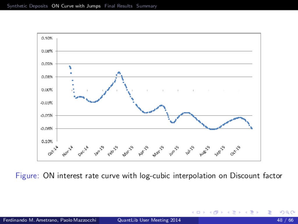
Problem The second critical point is the ON term structure: to obtain a good approximation of the basis, it is fundamental to build a good ON curve. Figure: ON interest rate curve with log-cubic interpolation on Discount factor Ferdinando M. Ametrano, Paolo Mazzocchi QuantLib User Meeting 2014 34 / 66
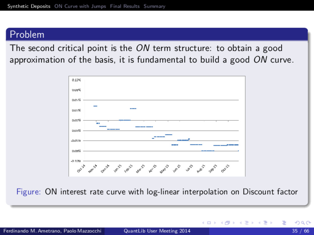
The second critical point is the ON term structure: to obtain a good approximation of the basis, it is fundamental to build a good ON curve. Figure: ON interest rate curve with log-linear interpolation on Discount factor Ferdinando M. Ametrano, Paolo Mazzocchi QuantLib User Meeting 2014 35 / 66
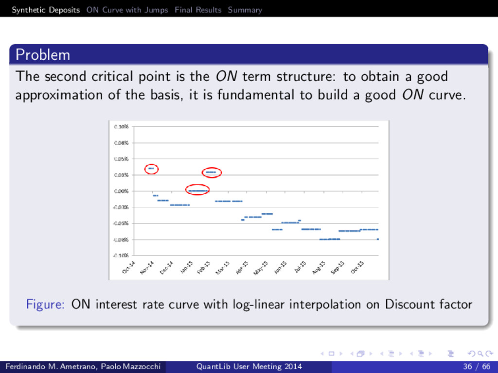
The second critical point is the ON term structure: to obtain a good approximation of the basis, it is fundamental to build a good ON curve. Figure: ON interest rate curve with log-linear interpolation on Discount factor Ferdinando M. Ametrano, Paolo Mazzocchi QuantLib User Meeting 2014 36 / 66
1 Synthetic Deposits The problem A first solution Residual problems 2 ON Curve with Jumps Jumps detection Jumps calculation 3 Final Results Forward rate curve using Synthetic Deposits Ferdinando M. Ametrano, Paolo Mazzocchi QuantLib User Meeting 2014 37 / 66
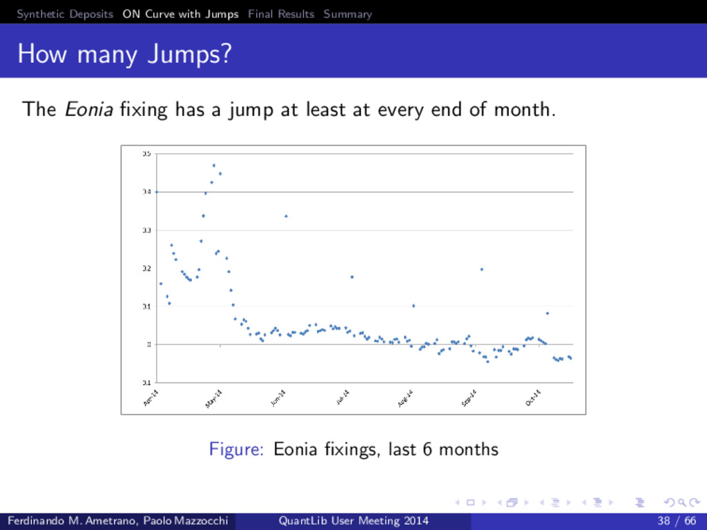
many Jumps? The Eonia fixing has a jump at least at every end of month. Figure: Eonia fixings, last 6 months Ferdinando M. Ametrano, Paolo Mazzocchi QuantLib User Meeting 2014 38 / 66
1 Synthetic Deposits The problem A first solution Residual problems 2 ON Curve with Jumps Jumps detection Jumps calculation 3 Final Results Forward rate curve using Synthetic Deposits Ferdinando M. Ametrano, Paolo Mazzocchi QuantLib User Meeting 2014 39 / 66
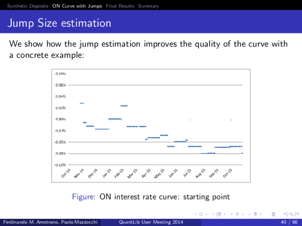
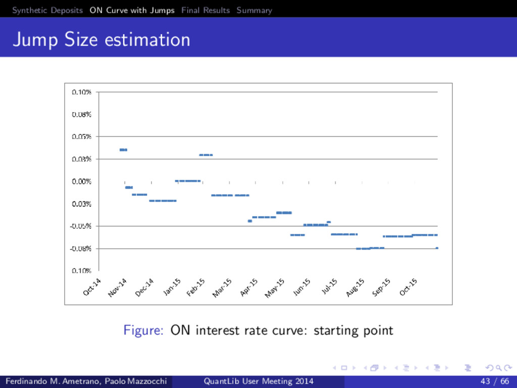
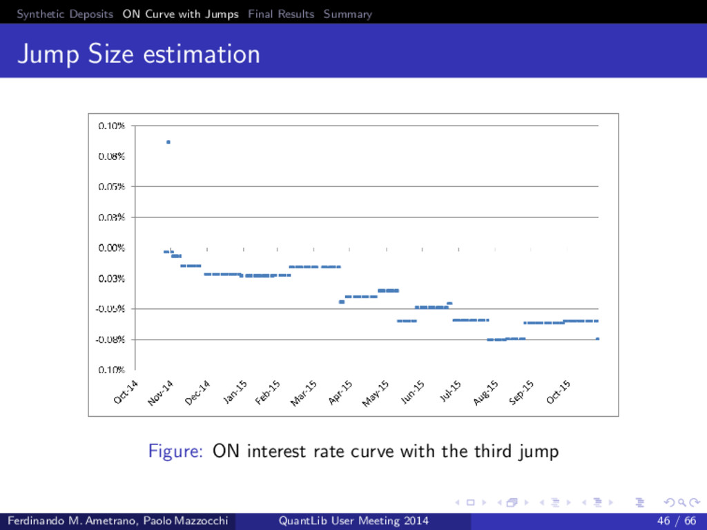
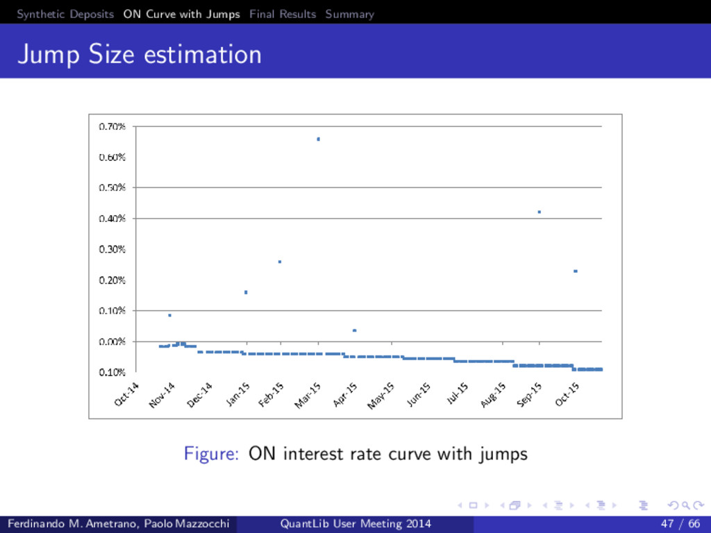
Size estimation We show how the jump estimation improves the quality of the curve with a concrete example: Figure: ON interest rate curve: starting point Ferdinando M. Ametrano, Paolo Mazzocchi QuantLib User Meeting 2014 40 / 66
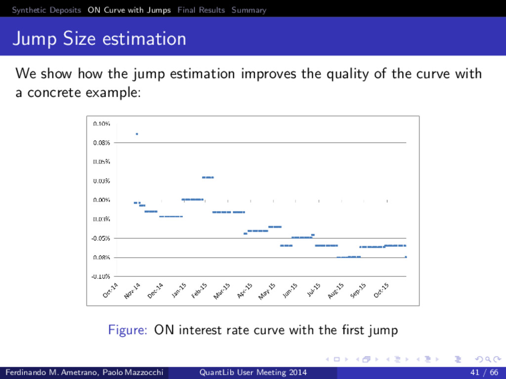
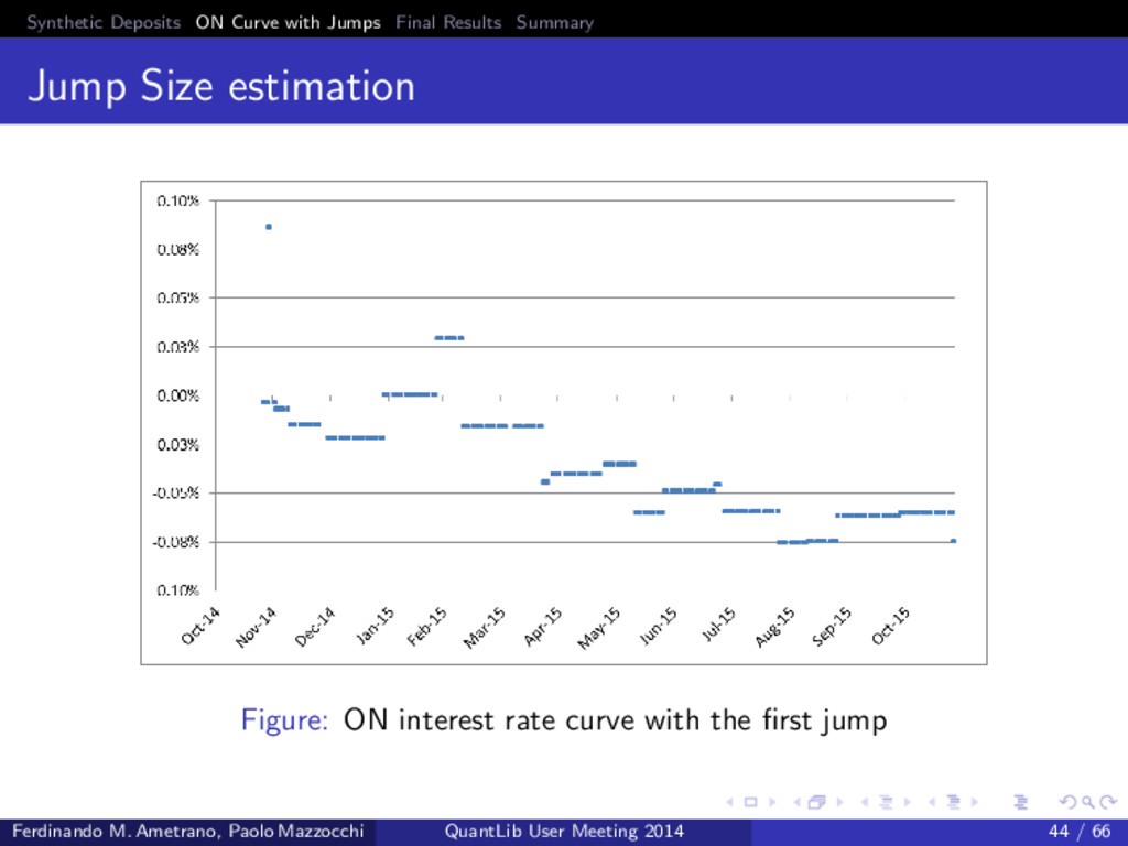
Size estimation We show how the jump estimation improves the quality of the curve with a concrete example: Figure: ON interest rate curve with the first jump Ferdinando M. Ametrano, Paolo Mazzocchi QuantLib User Meeting 2014 41 / 66
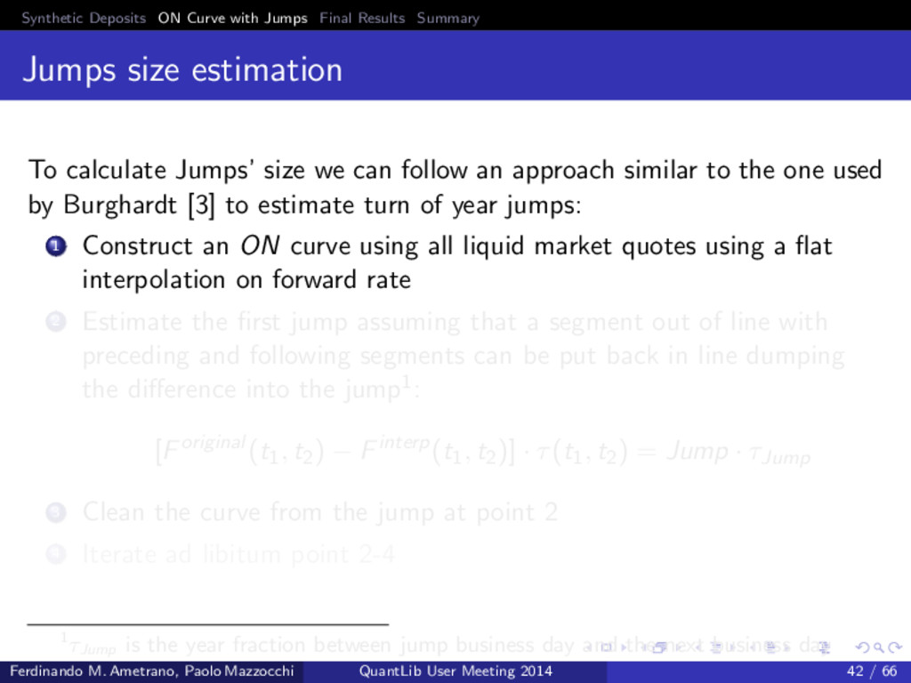
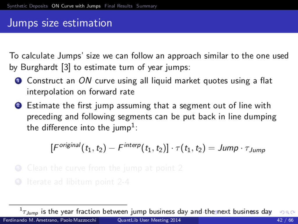
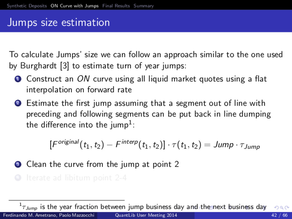
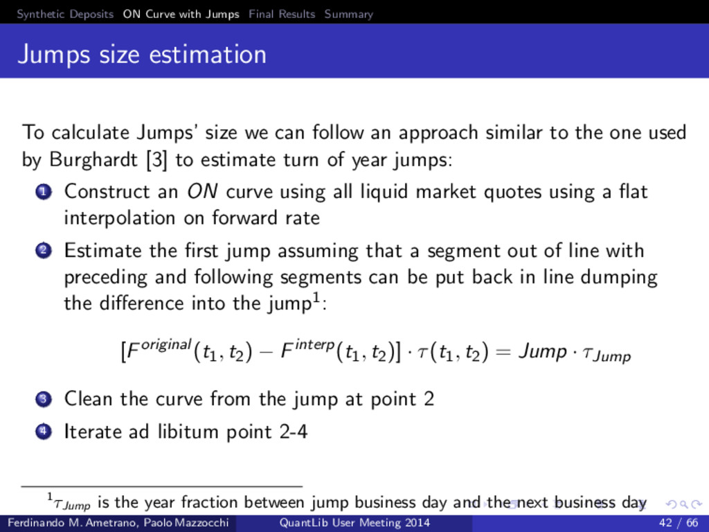
size estimation To calculate Jumps’ size we can follow an approach similar to the one used by Burghardt [3] to estimate turn of year jumps: 1 Construct an ON curve using all liquid market quotes using a flat interpolation on forward rate 2 Estimate the first jump assuming that a segment out of line with preceding and following segments can be put back in line dumping the difference into the jump1: [Foriginal (t1, t2) − Finterp(t1, t2)] · τ(t1, t2) = Jump · τJump 3 Clean the curve from the jump at point 2 4 Iterate ad libitum point 2-4 1τJump is the year fraction between jump business day and the next business day Ferdinando M. Ametrano, Paolo Mazzocchi QuantLib User Meeting 2014 42 / 66
size estimation To calculate Jumps’ size we can follow an approach similar to the one used by Burghardt [3] to estimate turn of year jumps: 1 Construct an ON curve using all liquid market quotes using a flat interpolation on forward rate 2 Estimate the first jump assuming that a segment out of line with preceding and following segments can be put back in line dumping the difference into the jump1: [Foriginal (t1, t2) − Finterp(t1, t2)] · τ(t1, t2) = Jump · τJump 3 Clean the curve from the jump at point 2 4 Iterate ad libitum point 2-4 1τJump is the year fraction between jump business day and the next business day Ferdinando M. Ametrano, Paolo Mazzocchi QuantLib User Meeting 2014 42 / 66
size estimation To calculate Jumps’ size we can follow an approach similar to the one used by Burghardt [3] to estimate turn of year jumps: 1 Construct an ON curve using all liquid market quotes using a flat interpolation on forward rate 2 Estimate the first jump assuming that a segment out of line with preceding and following segments can be put back in line dumping the difference into the jump1: [Foriginal (t1, t2) − Finterp(t1, t2)] · τ(t1, t2) = Jump · τJump 3 Clean the curve from the jump at point 2 4 Iterate ad libitum point 2-4 1τJump is the year fraction between jump business day and the next business day Ferdinando M. Ametrano, Paolo Mazzocchi QuantLib User Meeting 2014 42 / 66
size estimation To calculate Jumps’ size we can follow an approach similar to the one used by Burghardt [3] to estimate turn of year jumps: 1 Construct an ON curve using all liquid market quotes using a flat interpolation on forward rate 2 Estimate the first jump assuming that a segment out of line with preceding and following segments can be put back in line dumping the difference into the jump1: [Foriginal (t1, t2) − Finterp(t1, t2)] · τ(t1, t2) = Jump · τJump 3 Clean the curve from the jump at point 2 4 Iterate ad libitum point 2-4 1τJump is the year fraction between jump business day and the next business day Ferdinando M. Ametrano, Paolo Mazzocchi QuantLib User Meeting 2014 42 / 66
1 Synthetic Deposits The problem A first solution Residual problems 2 ON Curve with Jumps Jumps detection Jumps calculation 3 Final Results Forward rate curve using Synthetic Deposits Ferdinando M. Ametrano, Paolo Mazzocchi QuantLib User Meeting 2014 49 / 66
Deposits Construction We had 2 residual problems for construction of Synthetic Deposits: sub-optimal instruments selection wrong ON curve calculation Modelling ON jumps we fixed the ON curve and extrapolate B(0, x) in a robust way. Ferdinando M. Ametrano, Paolo Mazzocchi QuantLib User Meeting 2014 50 / 66
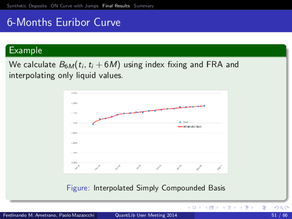
Euribor Curve Example We calculate B6M(ti , ti + 6M) using index fixing and FRA and interpolating only liquid values. Figure: Interpolated Simply Compounded Basis Ferdinando M. Ametrano, Paolo Mazzocchi QuantLib User Meeting 2014 51 / 66
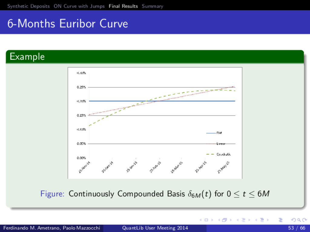
Euribor Curve Example Figure: Continuously Compounded Basis δ6M (t) for 0 ≤ t ≤ 6M Ferdinando M. Ametrano, Paolo Mazzocchi QuantLib User Meeting 2014 53 / 66
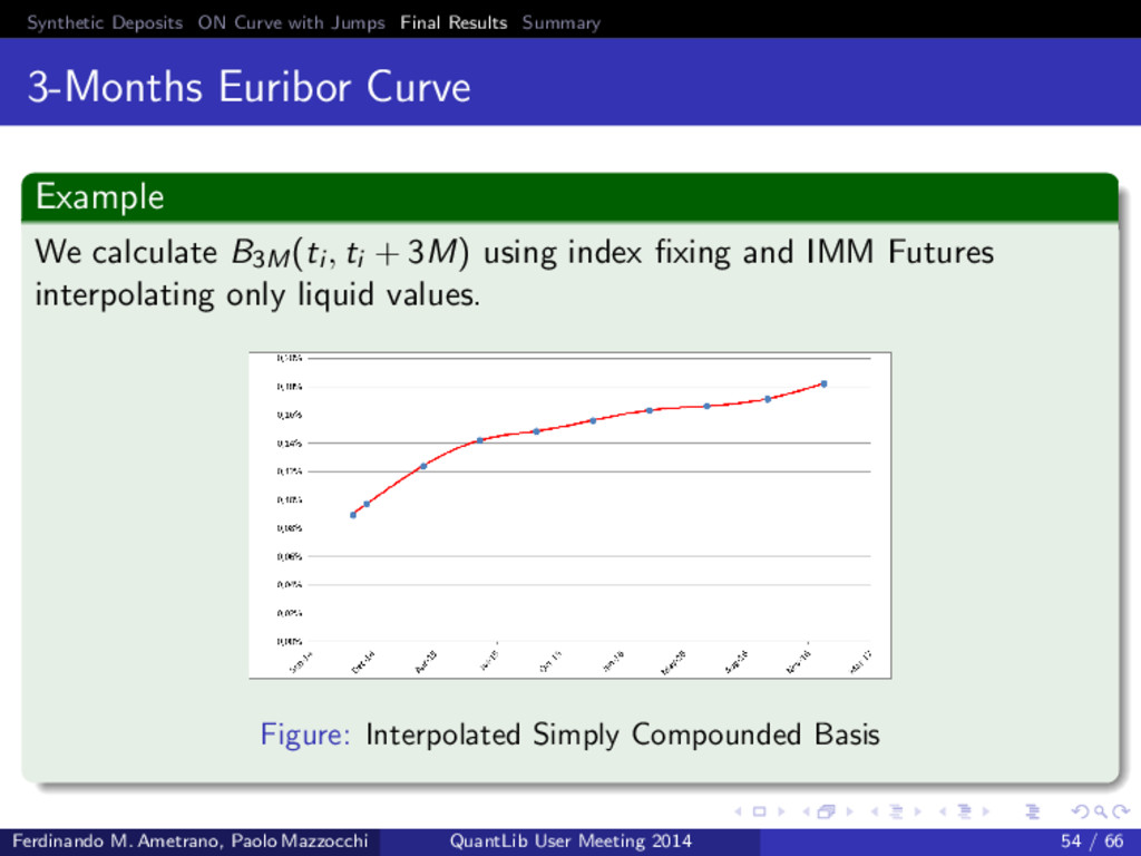
Euribor Curve Example We calculate B3M(ti , ti + 3M) using index fixing and IMM Futures interpolating only liquid values. Figure: Interpolated Simply Compounded Basis Ferdinando M. Ametrano, Paolo Mazzocchi QuantLib User Meeting 2014 54 / 66
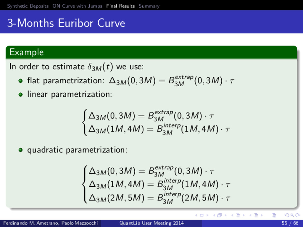
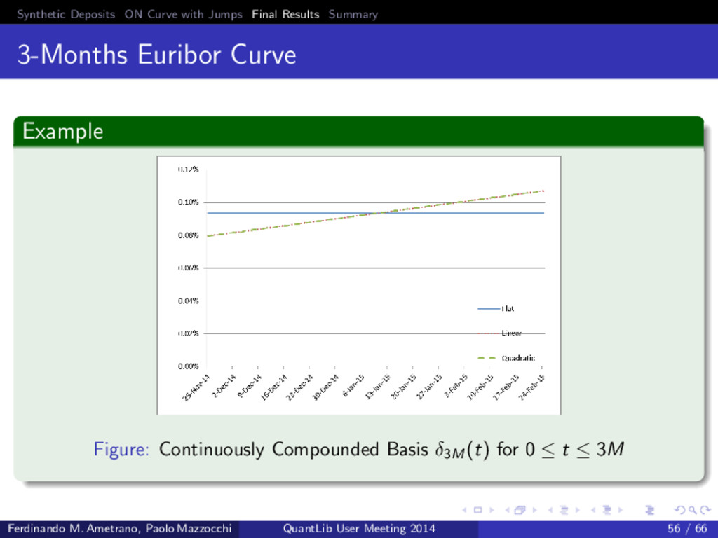
Euribor Curve Example Figure: Continuously Compounded Basis δ3M (t) for 0 ≤ t ≤ 3M Ferdinando M. Ametrano, Paolo Mazzocchi QuantLib User Meeting 2014 56 / 66
Euribor Curve Example The difference between initial and final results: Figure: Forward Euribor 6M Curve Ferdinando M. Ametrano, Paolo Mazzocchi QuantLib User Meeting 2014 57 / 66
Euribor Curve Example The difference between initial and final results: Figure: Forward Euribor 6M Curve Ferdinando M. Ametrano, Paolo Mazzocchi QuantLib User Meeting 2014 58 / 66
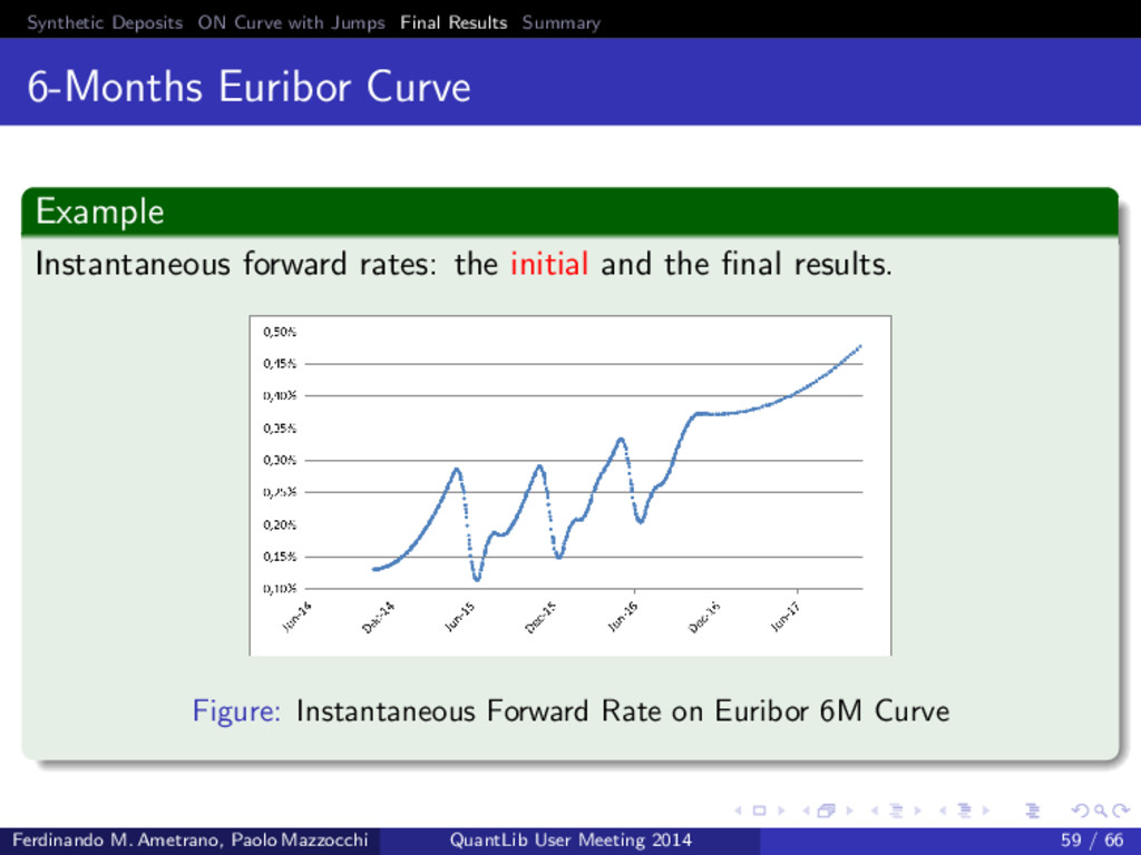
Euribor Curve Example Instantaneous forward rates: the initial and the final results. Figure: Instantaneous Forward Rate on Euribor 6M Curve Ferdinando M. Ametrano, Paolo Mazzocchi QuantLib User Meeting 2014 59 / 66
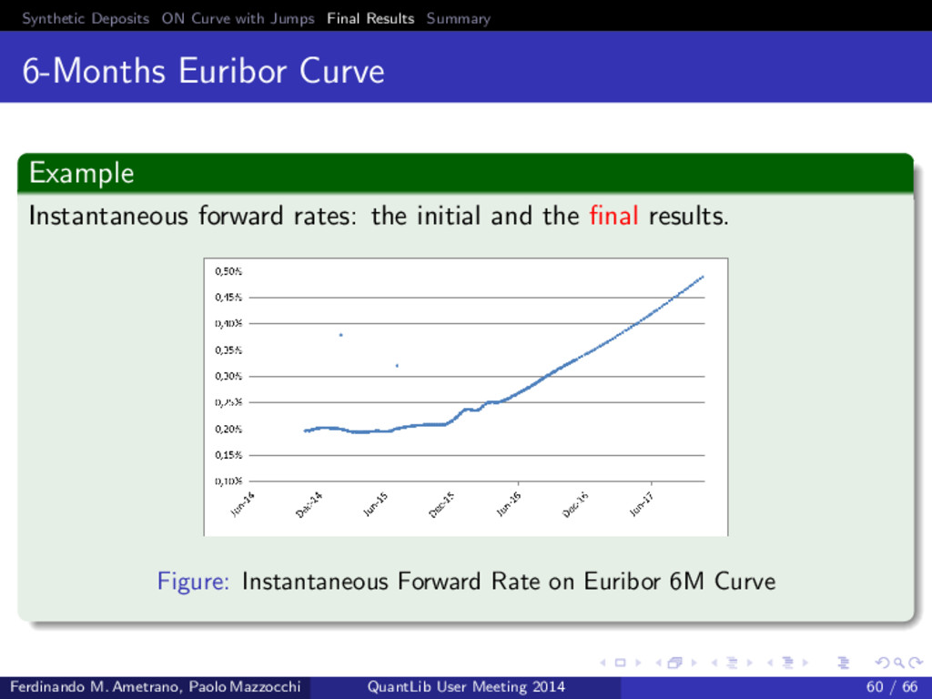
Euribor Curve Example Instantaneous forward rates: the initial and the final results. Figure: Instantaneous Forward Rate on Euribor 6M Curve Ferdinando M. Ametrano, Paolo Mazzocchi QuantLib User Meeting 2014 60 / 66
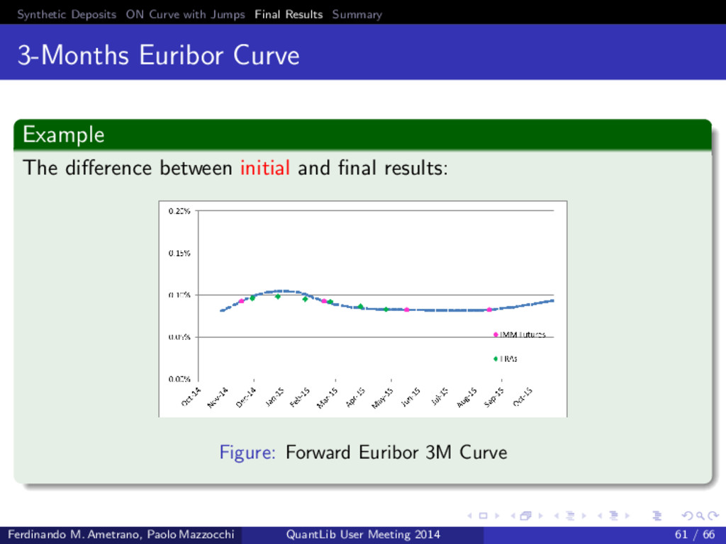
Euribor Curve Example The difference between initial and final results: Figure: Forward Euribor 3M Curve Ferdinando M. Ametrano, Paolo Mazzocchi QuantLib User Meeting 2014 61 / 66
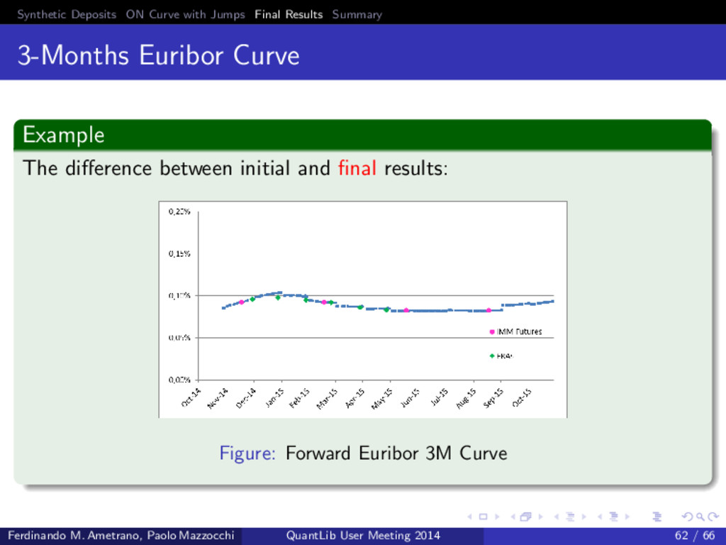
Euribor Curve Example The difference between initial and final results: Figure: Forward Euribor 3M Curve Ferdinando M. Ametrano, Paolo Mazzocchi QuantLib User Meeting 2014 62 / 66
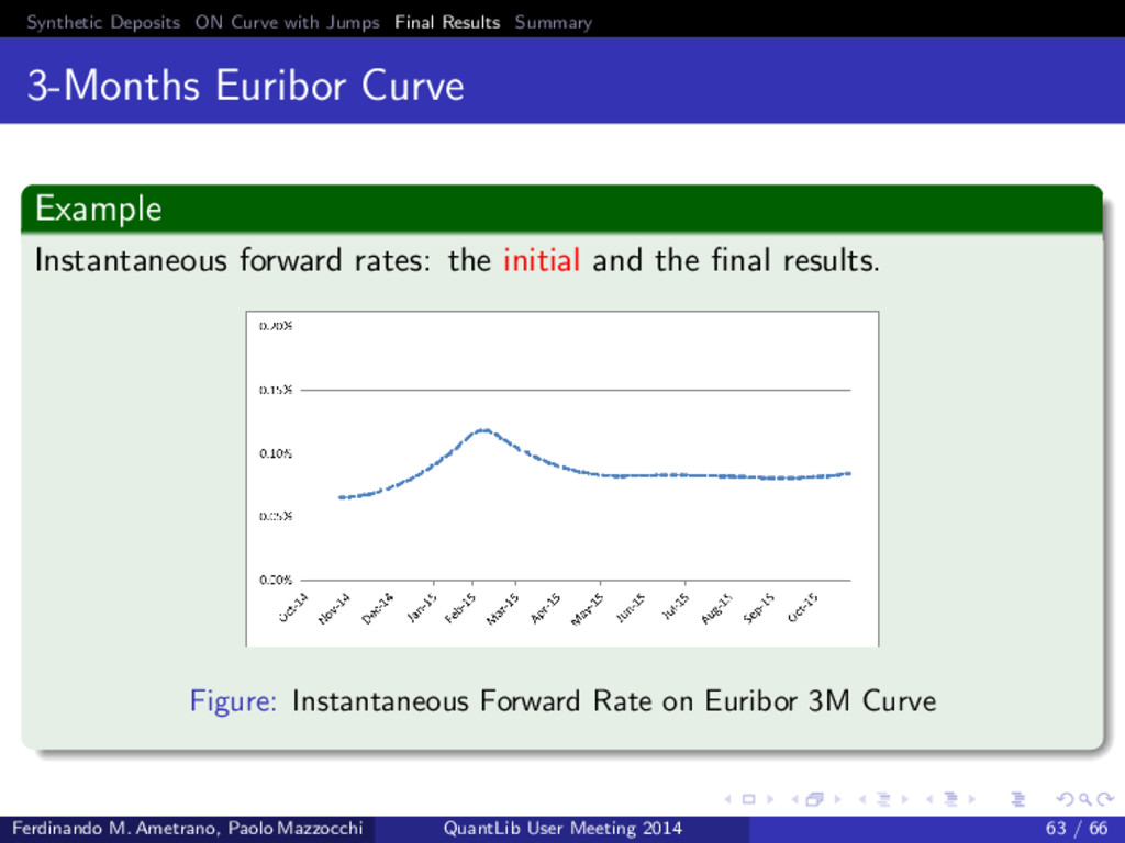
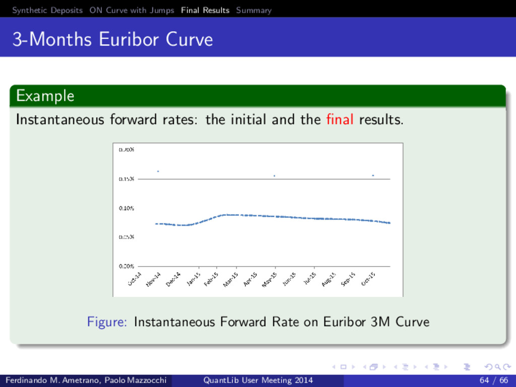
Euribor Curve Example Instantaneous forward rates: the initial and the final results. Figure: Instantaneous Forward Rate on Euribor 3M Curve Ferdinando M. Ametrano, Paolo Mazzocchi QuantLib User Meeting 2014 63 / 66
Euribor Curve Example Instantaneous forward rates: the initial and the final results. Figure: Instantaneous Forward Rate on Euribor 3M Curve Ferdinando M. Ametrano, Paolo Mazzocchi QuantLib User Meeting 2014 64 / 66
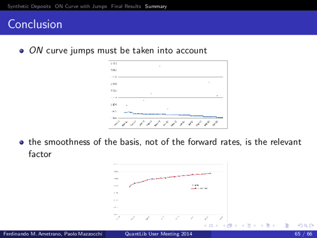
ON curve jumps must be taken into account the smoothness of the basis, not of the forward rates, is the relevant factor Ferdinando M. Ametrano, Paolo Mazzocchi QuantLib User Meeting 2014 65 / 66
F.M. Ametrano, M. Bianchetti Everything you always wanted to know about multiple interest rate curve bootstrapping but were afraid to ask. http://ssrn.com/abstract=2219548 SSRN, 2013. S. Schlenkrich,A. Miemiec Choosing the right spread. SSRN, 2014. G. Burghardt, S. Kirshner One good turn. CME Interest Rate Products Advanced Topics. Chicago: Chicago Mercatile Exchange,2002. Ferdinando M. Ametrano, Paolo Mazzocchi QuantLib User Meeting 2014 66 / 66