P r o g r e s s i n E a r t h S c i e n c e ? New Ideas / Hypotheses E 5 r 0 jUj p ðN/jUj jfj/jUj P 1D (k) ffiffiffiffiffiffiffiffiffiffiffiffiffiffiffiffiffiffiffiffiffiffiffiffiffi ffi N2 2 jUj2k2 q ffiffiffiffiffiffiffiffiffiffiffiffiffiffiffiffiffiffiffiffiffiffiffiffi jUj2k2 2 f2 q dk, (3) where k 5 (k, l) is now the wavenumber in the reference frame along and across the mean flow U and P 1D (k) 5 1 2p ð1‘ 2‘ jkj jkj P 2D (k, l) dl (4) is the effective one-dimensional (1D) topographic spectrum. Hence, the wave radiation from 2D topogra- phy reduces to an equivalent problem of wave radiation from 1D topography with the effective spectrum given by P1D (k). The effective 1D spectrum captures the effects of 2D c. Bottom topography Simulations are configured with multiscale topogra- phy characterized by small-scale abyssal hills a few ki- lometers wide based on multibeam observations from Drake Passage. The topographic spectrum associated with abyssal hills is well described by an anisotropic parametric representation proposed by Goff and Jordan (1988): P 2D (k, l) 5 2pH2(m 2 2) k 0 l 0 1 1 k2 k2 0 1 l2 l2 0 !2m/2 , (5) where k0 and l0 set the wavenumbers of the large hills, m is the high-wavenumber spectral slope, related to the pa- FIG. 3. Averaged profiles of (left) stratification (s21) and (right) flow speed (m s21) in the bottom 2 km from observations (gray), initial condition in the simulations (black), and final state in 2D (blue) and 3D (red) simulations.
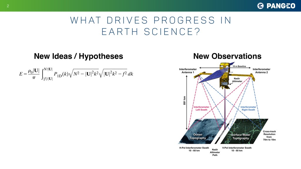
P r o g r e s s i n E a r t h S c i e n c e ? New Ideas / Hypotheses New Observations E 5 r 0 jUj p ðN/jUj jfj/jUj P 1D (k) ffiffiffiffiffiffiffiffiffiffiffiffiffiffiffiffiffiffiffiffiffiffiffiffiffi ffi N2 2 jUj2k2 q ffiffiffiffiffiffiffiffiffiffiffiffiffiffiffiffiffiffiffiffiffiffiffiffi jUj2k2 2 f2 q dk, (3) where k 5 (k, l) is now the wavenumber in the reference frame along and across the mean flow U and P 1D (k) 5 1 2p ð1‘ 2‘ jkj jkj P 2D (k, l) dl (4) is the effective one-dimensional (1D) topographic spectrum. Hence, the wave radiation from 2D topogra- phy reduces to an equivalent problem of wave radiation from 1D topography with the effective spectrum given by P1D (k). The effective 1D spectrum captures the effects of 2D c. Bottom topography Simulations are configured with multiscale topogra- phy characterized by small-scale abyssal hills a few ki- lometers wide based on multibeam observations from Drake Passage. The topographic spectrum associated with abyssal hills is well described by an anisotropic parametric representation proposed by Goff and Jordan (1988): P 2D (k, l) 5 2pH2(m 2 2) k 0 l 0 1 1 k2 k2 0 1 l2 l2 0 !2m/2 , (5) where k0 and l0 set the wavenumbers of the large hills, m is the high-wavenumber spectral slope, related to the pa- FIG. 3. Averaged profiles of (left) stratification (s21) and (right) flow speed (m s21) in the bottom 2 km from observations (gray), initial condition in the simulations (black), and final state in 2D (blue) and 3D (red) simulations.
P r o g r e s s i n E a r t h S c i e n c e ? New Ideas / Hypotheses New Observations E 5 r 0 jUj p ðN/jUj jfj/jUj P 1D (k) ffiffiffiffiffiffiffiffiffiffiffiffiffiffiffiffiffiffiffiffiffiffiffiffiffi ffi N2 2 jUj2k2 q ffiffiffiffiffiffiffiffiffiffiffiffiffiffiffiffiffiffiffiffiffiffiffiffi jUj2k2 2 f2 q dk, (3) where k 5 (k, l) is now the wavenumber in the reference frame along and across the mean flow U and P 1D (k) 5 1 2p ð1‘ 2‘ jkj jkj P 2D (k, l) dl (4) is the effective one-dimensional (1D) topographic spectrum. Hence, the wave radiation from 2D topogra- phy reduces to an equivalent problem of wave radiation from 1D topography with the effective spectrum given by P1D (k). The effective 1D spectrum captures the effects of 2D c. Bottom topography Simulations are configured with multiscale topogra- phy characterized by small-scale abyssal hills a few ki- lometers wide based on multibeam observations from Drake Passage. The topographic spectrum associated with abyssal hills is well described by an anisotropic parametric representation proposed by Goff and Jordan (1988): P 2D (k, l) 5 2pH2(m 2 2) k 0 l 0 1 1 k2 k2 0 1 l2 l2 0 !2m/2 , (5) where k0 and l0 set the wavenumbers of the large hills, m is the high-wavenumber spectral slope, related to the pa- FIG. 3. Averaged profiles of (left) stratification (s21) and (right) flow speed (m s21) in the bottom 2 km from observations (gray), initial condition in the simulations (black), and final state in 2D (blue) and 3D (red) simulations.
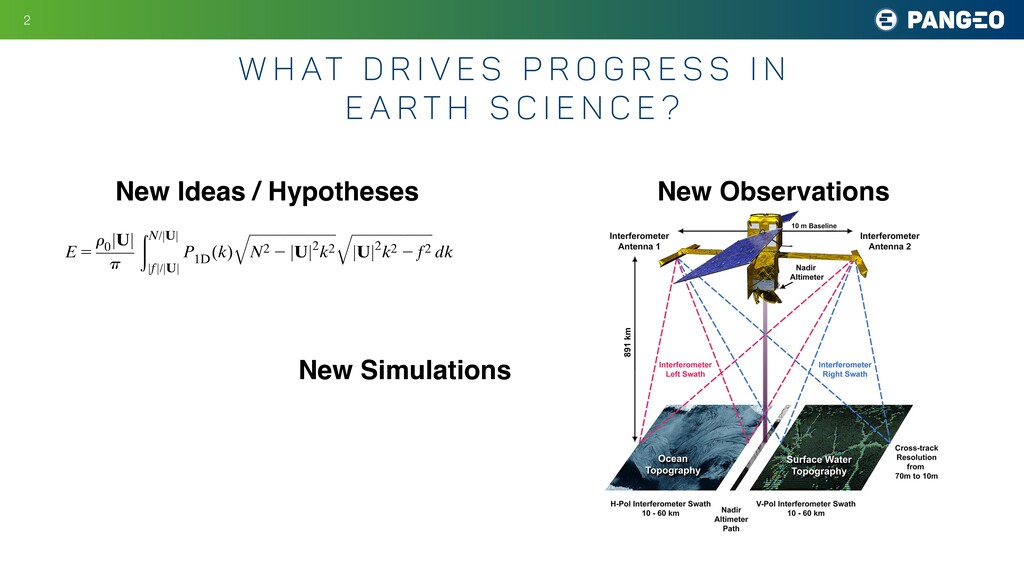
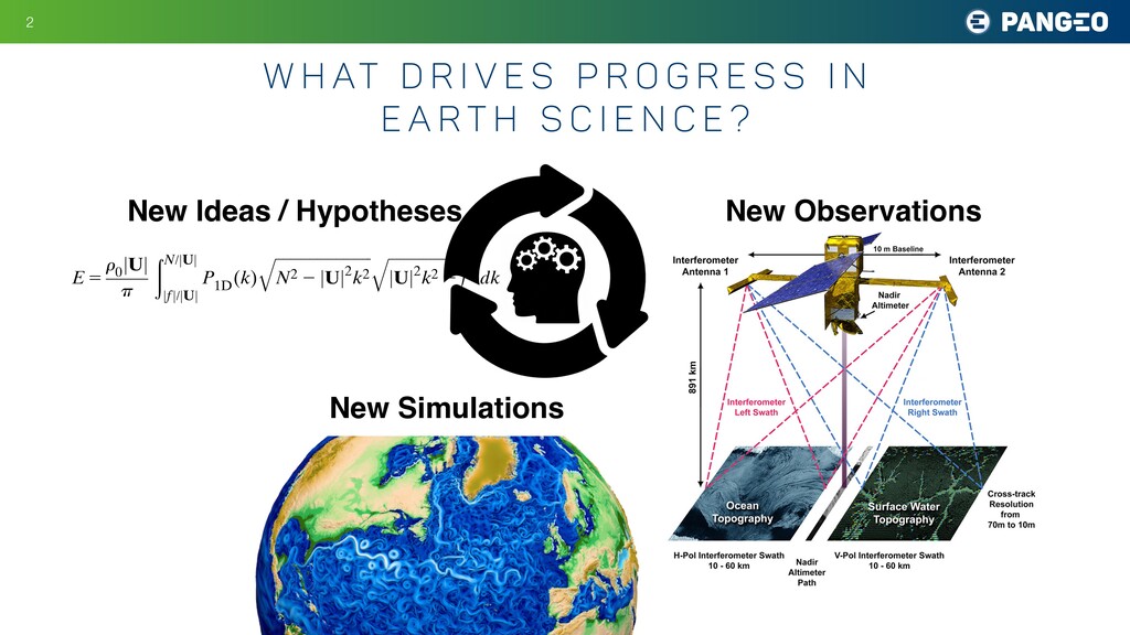
P r o g r e s s i n E a r t h S c i e n c e ? New Ideas / Hypotheses New Observations New Simulations E 5 r 0 jUj p ðN/jUj jfj/jUj P 1D (k) ffiffiffiffiffiffiffiffiffiffiffiffiffiffiffiffiffiffiffiffiffiffiffiffiffi ffi N2 2 jUj2k2 q ffiffiffiffiffiffiffiffiffiffiffiffiffiffiffiffiffiffiffiffiffiffiffiffi jUj2k2 2 f2 q dk, (3) where k 5 (k, l) is now the wavenumber in the reference frame along and across the mean flow U and P 1D (k) 5 1 2p ð1‘ 2‘ jkj jkj P 2D (k, l) dl (4) is the effective one-dimensional (1D) topographic spectrum. Hence, the wave radiation from 2D topogra- phy reduces to an equivalent problem of wave radiation from 1D topography with the effective spectrum given by P1D (k). The effective 1D spectrum captures the effects of 2D c. Bottom topography Simulations are configured with multiscale topogra- phy characterized by small-scale abyssal hills a few ki- lometers wide based on multibeam observations from Drake Passage. The topographic spectrum associated with abyssal hills is well described by an anisotropic parametric representation proposed by Goff and Jordan (1988): P 2D (k, l) 5 2pH2(m 2 2) k 0 l 0 1 1 k2 k2 0 1 l2 l2 0 !2m/2 , (5) where k0 and l0 set the wavenumbers of the large hills, m is the high-wavenumber spectral slope, related to the pa- FIG. 3. Averaged profiles of (left) stratification (s21) and (right) flow speed (m s21) in the bottom 2 km from observations (gray), initial condition in the simulations (black), and final state in 2D (blue) and 3D (red) simulations.
P r o g r e s s i n E a r t h S c i e n c e ? New Ideas / Hypotheses New Observations New Simulations E 5 r 0 jUj p ðN/jUj jfj/jUj P 1D (k) ffiffiffiffiffiffiffiffiffiffiffiffiffiffiffiffiffiffiffiffiffiffiffiffiffi ffi N2 2 jUj2k2 q ffiffiffiffiffiffiffiffiffiffiffiffiffiffiffiffiffiffiffiffiffiffiffiffi jUj2k2 2 f2 q dk, (3) where k 5 (k, l) is now the wavenumber in the reference frame along and across the mean flow U and P 1D (k) 5 1 2p ð1‘ 2‘ jkj jkj P 2D (k, l) dl (4) is the effective one-dimensional (1D) topographic spectrum. Hence, the wave radiation from 2D topogra- phy reduces to an equivalent problem of wave radiation from 1D topography with the effective spectrum given by P1D (k). The effective 1D spectrum captures the effects of 2D c. Bottom topography Simulations are configured with multiscale topogra- phy characterized by small-scale abyssal hills a few ki- lometers wide based on multibeam observations from Drake Passage. The topographic spectrum associated with abyssal hills is well described by an anisotropic parametric representation proposed by Goff and Jordan (1988): P 2D (k, l) 5 2pH2(m 2 2) k 0 l 0 1 1 k2 k2 0 1 l2 l2 0 !2m/2 , (5) where k0 and l0 set the wavenumbers of the large hills, m is the high-wavenumber spectral slope, related to the pa- FIG. 3. Averaged profiles of (left) stratification (s21) and (right) flow speed (m s21) in the bottom 2 km from observations (gray), initial condition in the simulations (black), and final state in 2D (blue) and 3D (red) simulations.
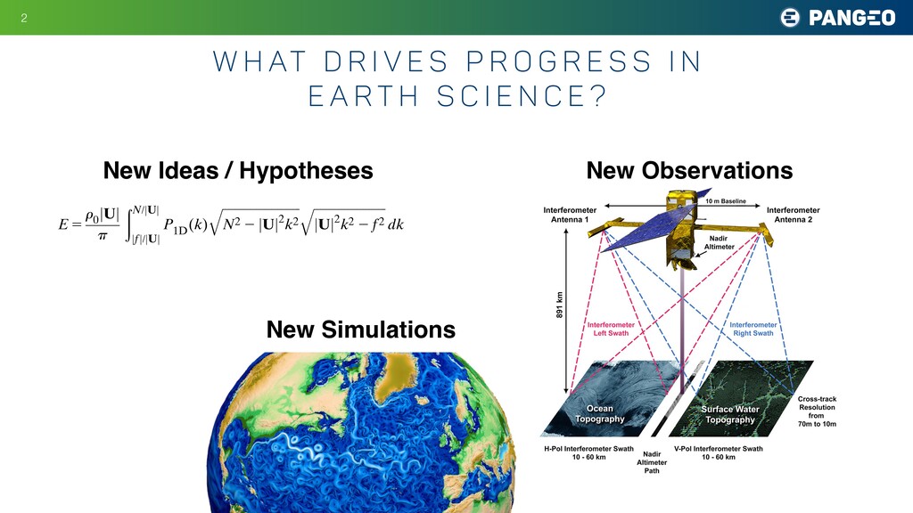
P r o g r e s s i n E a r t h S c i e n c e ? New Ideas / Hypotheses New Observations New Simulations E 5 r 0 jUj p ðN/jUj jfj/jUj P 1D (k) ffiffiffiffiffiffiffiffiffiffiffiffiffiffiffiffiffiffiffiffiffiffiffiffiffi ffi N2 2 jUj2k2 q ffiffiffiffiffiffiffiffiffiffiffiffiffiffiffiffiffiffiffiffiffiffiffiffi jUj2k2 2 f2 q dk, (3) where k 5 (k, l) is now the wavenumber in the reference frame along and across the mean flow U and P 1D (k) 5 1 2p ð1‘ 2‘ jkj jkj P 2D (k, l) dl (4) is the effective one-dimensional (1D) topographic spectrum. Hence, the wave radiation from 2D topogra- phy reduces to an equivalent problem of wave radiation from 1D topography with the effective spectrum given by P1D (k). The effective 1D spectrum captures the effects of 2D c. Bottom topography Simulations are configured with multiscale topogra- phy characterized by small-scale abyssal hills a few ki- lometers wide based on multibeam observations from Drake Passage. The topographic spectrum associated with abyssal hills is well described by an anisotropic parametric representation proposed by Goff and Jordan (1988): P 2D (k, l) 5 2pH2(m 2 2) k 0 l 0 1 1 k2 k2 0 1 l2 l2 0 !2m/2 , (5) where k0 and l0 set the wavenumbers of the large hills, m is the high-wavenumber spectral slope, related to the pa- FIG. 3. Averaged profiles of (left) stratification (s21) and (right) flow speed (m s21) in the bottom 2 km from observations (gray), initial condition in the simulations (black), and final state in 2D (blue) and 3D (red) simulations.
W h at S c i e n c e d o w e w a n t t o d o w i t h C l i m at e D ata? manuscript submitted to Journal of Advances in Modeling Earth Systems (JAMES) Input: SSH Day 20 Day 0 2x(32x32) Output: SSH Day 10 32x32 … + + + + + + Global Avg. pool Fully Connected layer(1024) Conv2D 2,32 Conv2D 64,128 Conv2D 32,64 Conv2D 128,256 + x Identity X Add Conv2D Batch Norm Leaky ReLU Conv2D Batch Norm Leaky ReLU Conv2D Batch Norm Add X Leaky ReLU Conv2D, BatchNorm Leaky ReLu, MaxPool Conv2D 256, 512 + + Conv2D M,N … … y y=max(0.1x,x) Leaky ReLU
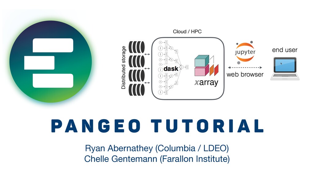
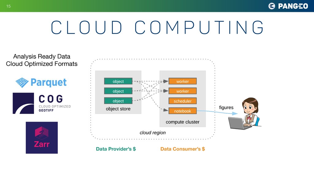
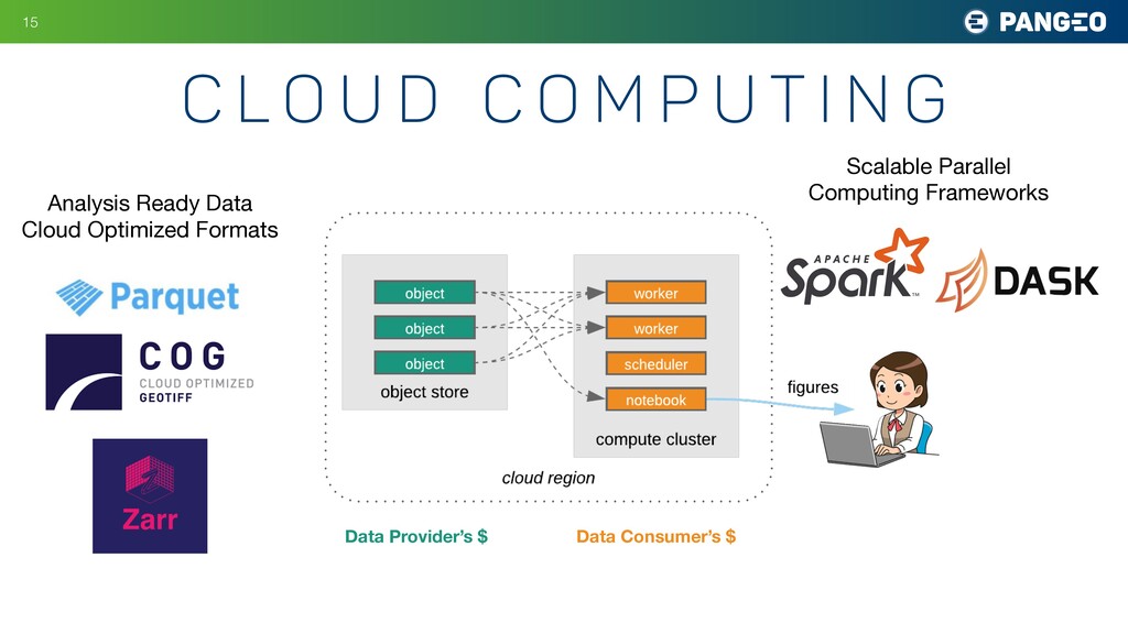
i t e c t u r e Jupyter for interactive access remote systems Cloud / HPC Xarray provides data structures and intuitive interface for interacting with datasets Parallel computing system allows users deploy clusters of compute nodes for data processing. Dask tells the nodes what to do. Distributed storage “Analysis Ready Data” stored on globally-available distributed storage.
python, xarray, dask, etc. on your computer. • Install Pangeo on your own cluster: instructions at http://pangeo.io/setup_guides/hpc.html • Use Pangeo on NCAR’s Cheyenne: https://discourse.pangeo.io/t/jupyterhub-access-on-cheyenne/253 • Use one of our cloud-based Jupyterhubs: http://pangeo.io/deployments.html Note: we don’t really have funding (yet) to support the whole world • Deploy your own Pangeo environment in the cloud http://pangeo.io/setup_guides/cloud.html Costs $ - talk to your program manager! H o w c a n y o u U S E Pa n g e o ? !22
way to calculate X? Where can I find dataset Y? • Attend a weekly telecon or working-group meeting: pangeo.io/meeting-notes.html • Create your own binders and add them to our gallery: github.com/pangeo-gallery (website still under development) • Put data on the cloud: github.com/pangeo-data/pangeo-datastore (Note: cloud storage costs money! We are working with cloud providers, funding agencies, and data providers to bring more analysis-ready data to the cloud in a sustainable way.) H o w c a n y o u C o n t r i b u t e ? !23