Causal data science

Transcript

1. Causal data science: A guide to the crucial ‘why’ in your analysis Subhasish Misra Staff Data Scientist @Walmart Labs * Pic source – www.neatosource.com.
2. * Source- Chocolate Consumption, Cognitive Function, and Nobel Laureates Franz H. Messerli, M.D, New England journal of medicine - 2012
3. Correlation is not always causation, but then what is causation ? * Source - https://xkcd.com/552/
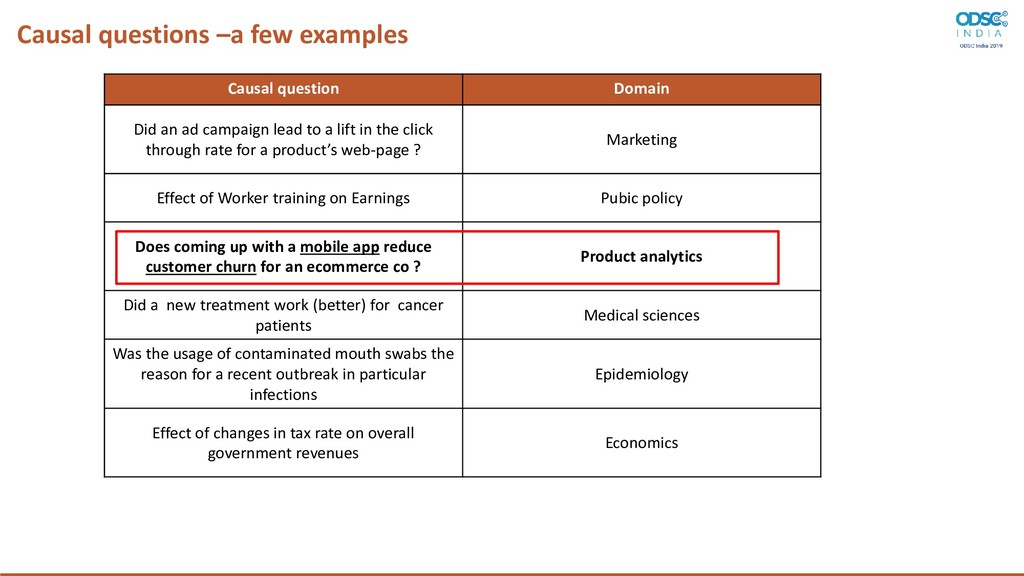
4. Causal questions –a few examples Causal question Domain Did an ad campaign lead to a lift in the click through rate for a product’s web-page ? Marketing Effect of Worker training on Earnings Pubic policy Does coming up with a mobile app reduce customer churn for an ecommerce co ? Product analytics Did a new treatment work (better) for cancer patients Medical sciences Was the usage of contaminated mouth swabs the reason for a recent outbreak in particular infections Epidemiology Effect of changes in tax rate on overall government revenues Economics
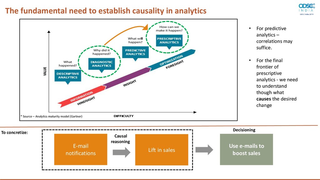
5. The fundamental need to establish causality in analytics * Source – Analytics maturity model (Gartner) • For predictive analytics – correlations may suffice. • For the final frontier of prescriptive analytics - we need to understand though what causes the desired change To concretize: E-mail notifications Lift in sales Use e-mails to boost sales Causal reasoning Decisioning
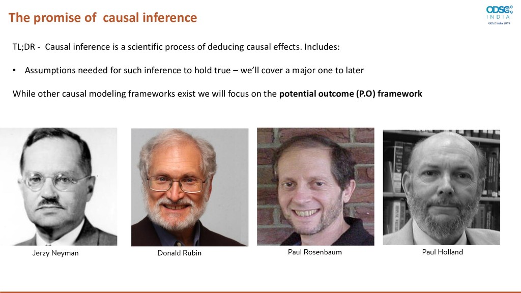
6. The promise of causal inference TL;DR - Causal inference is a scientific process of deducing causal effects. Includes: • Assumptions needed for such inference to hold true – we’ll cover a major one to later While other causal modeling frameworks exist we will focus on the potential outcome (P.O) framework
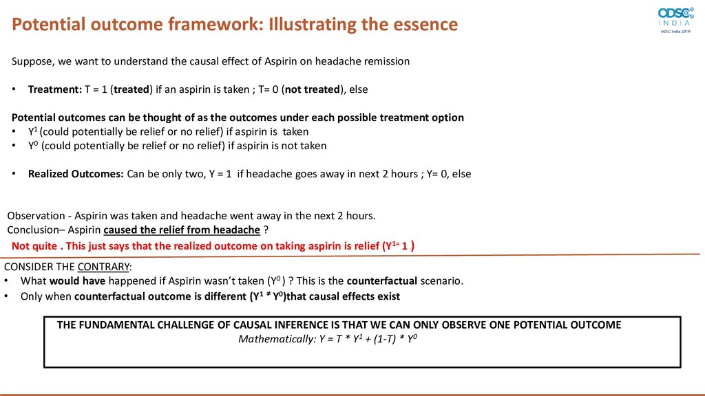
7. CONSIDER THE CONTRARY: • What would have happened if Aspirin wasn’t taken (Y0 ) ? This is the counterfactual scenario. • Only when counterfactual outcome is different (Y1 ≠ Y0)that causal effects exist THE FUNDAMENTAL CHALLENGE OF CAUSAL INFERENCE IS THAT WE CAN ONLY OBSERVE ONE POTENTIAL OUTCOME Mathematically: Y = T * Y1 + (1-T) * Y0 Potential outcome framework: Illustrating the essence Suppose, we want to understand the causal effect of Aspirin on headache remission • Treatment: T = 1 (treated) if an aspirin is taken ; T= 0 (not treated), else Potential outcomes can be thought of as the outcomes under each possible treatment option • Y1 (could potentially be relief or no relief) if aspirin is taken • Y0 (could potentially be relief or no relief) if aspirin is not taken • Realized Outcomes: Can be only two, Y = 1 if headache goes away in next 2 hours ; Y= 0, else Not quite . This just says that the realized outcome on taking aspirin is relief (Y1= 1 ) Observation - Aspirin was taken and headache went away in the next 2 hours. Conclusion– Aspirin caused the relief from headache ?
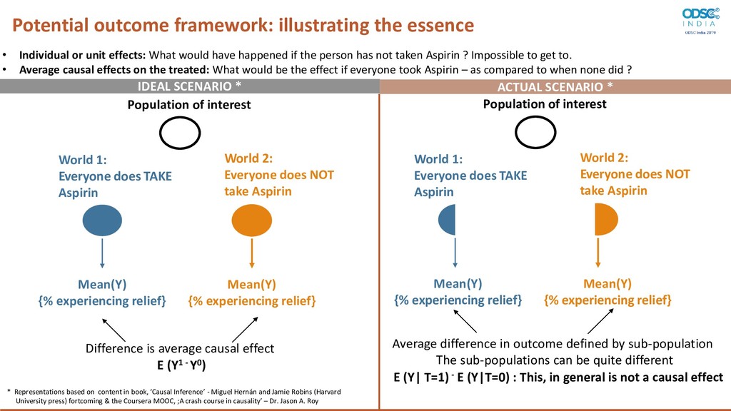
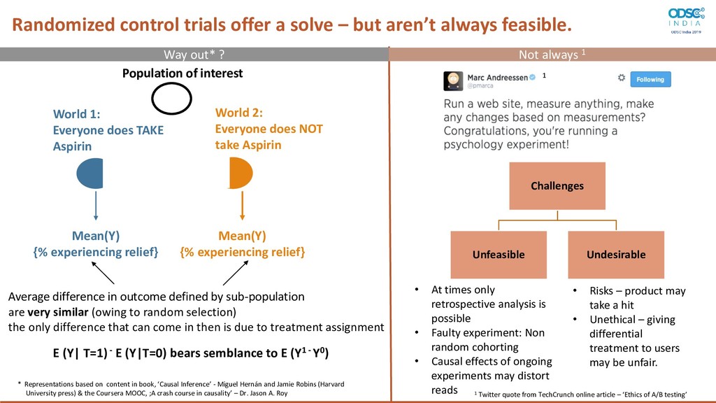
8. Potential outcome framework: illustrating the essence • Individual or unit effects: What would have happened if the person has not taken Aspirin ? Impossible to get to. • Average causal effects on the treated: What would be the effect if everyone took Aspirin – as compared to when none did ? Population of interest World 2: Everyone does NOT take Aspirin World 1: Everyone does TAKE Aspirin Mean(Y) {% experiencing relief} Mean(Y) {% experiencing relief} Difference is average causal effect IDEAL SCENARIO * ACTUAL SCENARIO * Population of interest World 2: Everyone does NOT take Aspirin World 1: Everyone does TAKE Aspirin Mean(Y) {% experiencing relief} Mean(Y) {% experiencing relief} Average difference in outcome defined by sub-population The sub-populations can be quite different E (Y1 - Y0) E (Y| T=1) - E (Y|T=0) : This, in general is not a causal effect * Representations based on content in book, ‘Causal Inference’ - Miguel Hernán and Jamie Robins (Harvard University press) fortcoming & the Coursera MOOC, ;A crash course in causality’ – Dr. Jason A. Roy
9. Randomized control trials offer a solve – but aren’t always feasible. World 2: Everyone does NOT take Aspirin World 1: Everyone does TAKE Aspirin Mean(Y) {% experiencing relief} Mean(Y) {% experiencing relief} Average difference in outcome defined by sub-population are very similar (owing to random selection) the only difference that can come in then is due to treatment assignment E (Y| T=1) - E (Y|T=0) bears semblance to E (Y1 - Y0) Way out* ? Not always 1 Population of interest Challenges Unfeasible Undesirable • At times only retrospective analysis is possible • Faulty experiment: Non random cohorting • Causal effects of ongoing experiments may distort reads • Risks – product may take a hit • Unethical – giving differential treatment to users may be unfair. 1 1 Twitter quote from TechCrunch online article – ‘Ethics of A/B testing’ * Representations based on content in book, ‘Causal Inference’ - Miguel Hernán and Jamie Robins (Harvard University press) & the Coursera MOOC, ;A crash course in causality’ – Dr. Jason A. Roy
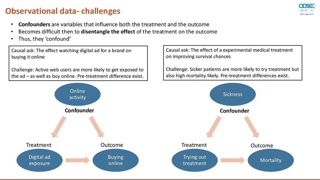
10. Observational data- challenges • Confounders are variables that influence both the treatment and the outcome • Becomes difficult then to disentangle the effect of the treatment on the outcome • Thus, they ‘confound’ Online activity Buying online Digital ad exposure Treatment Outcome Confounder Causal ask: The effect watching digital ad for a brand on buying it online Challenge: Active web users are more likely to get exposed to the ad – as well as buy online. Pre-treatment difference exist. Sickness Mortality Trying out treatment Causal ask: The effect of a experimental medical treatment on improving survival chances Challenge: Sicker patients are more likely to try treatment but also high mortality likely. Pre-treatment differences exist. Confounder Treatment Outcome
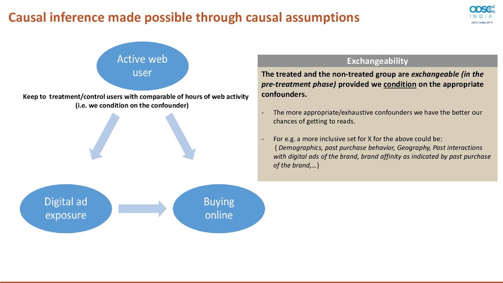
11. The treated and the non-treated group are exchangeable (in the pre-treatment phase) provided we condition on the appropriate confounders. - The more appropriate/exhaustive confounders we have the better our chances of getting to reads. - For e.g. a more inclusive set for X for the above could be: { Demographics, past purchase behavior, Geography, Past interactions with digital ads of the brand, brand affinity as indicated by past purchase of the brand,…} Causal inference made possible through causal assumptions Keep to treatment/control users with comparable of hours of web activity (i.e. we condition on the confounder) Exchangeability
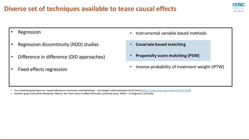
12. Diverse set of techniques available to tease causal effects • Regression • Regression discontinuity (RDD) studies • Difference in difference (DID approaches) • Fixed effects regression • Instrumental variable based methods • Covariate based matching • Propensity score matching (PSM) • Inverse probability of treatment weight (IPTW) • For a brief but great intro see ‘Causal inference in Economics and Marketing’ – by Google’s chief economist Hal R Varian (https://www.pnas.org/content/113/27/7310) • Another great read will be Mastering ’Metrics: the from Cause to effect (Princeton university press, 2014) – J.D Angrist & J.S.Pischke
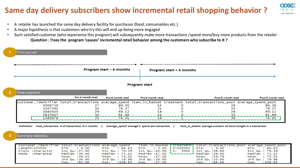
13. Same day delivery subscribers show incremental retail shopping behavior ? • A retailer has launched the same day delivery facility for purchases (food, consumables etc.) • A major hypothesis is that customers who try this will end up being more engaged • Such satisfied customer (who experience this program) will subsequently make more transactions /spend more/buy more products from the retailer Question : Does the program ‘causes’ incremental retail behavior among the customers who subscribe to it ?
14. Selection bias: Typically subscribers are among the better customers Number of transactions (past 6 months) Average dollar spend per transaction (past 6 months) 30 35 70$ 75$
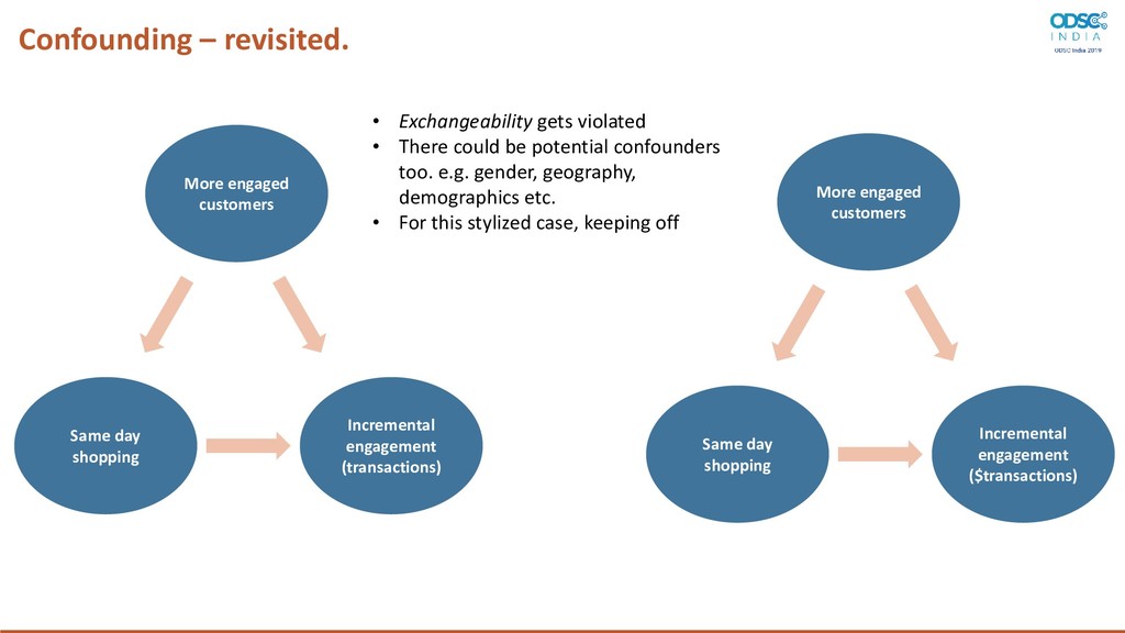
15. Confounding – revisited. Same day shopping Incremental engagement (transactions) More engaged customers Same day shopping Incremental engagement ($transactions) More engaged customers • Exchangeability gets violated • There could be potential confounders too. e.g. gender, geography, demographics etc. • For this stylized case, keeping off
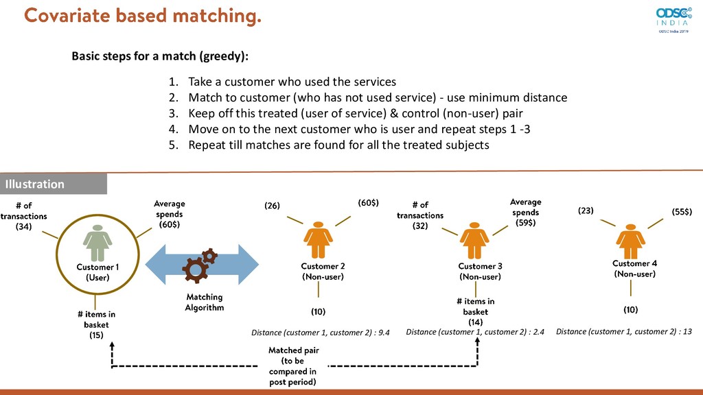
16. Basic steps for a match (greedy): 1. Take a customer who used the services 2. Match to customer (who has not used service) - use minimum distance 3. Keep off this treated (user of service) & control (non-user) pair 4. Move on to the next customer who is user and repeat steps 1 -3 5. Repeat till matches are found for all the treated subjects Distance (customer 1, customer 2) : 9.4 Distance (customer 1, customer 2) : 2.4 Distance (customer 1, customer 2) : 13 Illustration
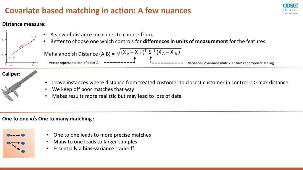
17. Covariate based matching in action: A few nuances Distance measure: One to one v/s One to many matching : • A slew of distance measures to choose from. • Better to choose one which controls for differences in units of measurement for the features. • One to one leads to more precise matches • Many to one leads to larger samples • Essentially a bias-variance tradeoff • Leave instances where distance from treated customer to closest customer in control is > max distance • We keep off poor matches that way • Makes results more realistic but may lead to loss of data Variance-Covariance matrix. Ensures appropriate scaling Vector representation of point A Mahalanobish Distance (A,B) = Caliper:
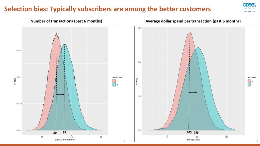
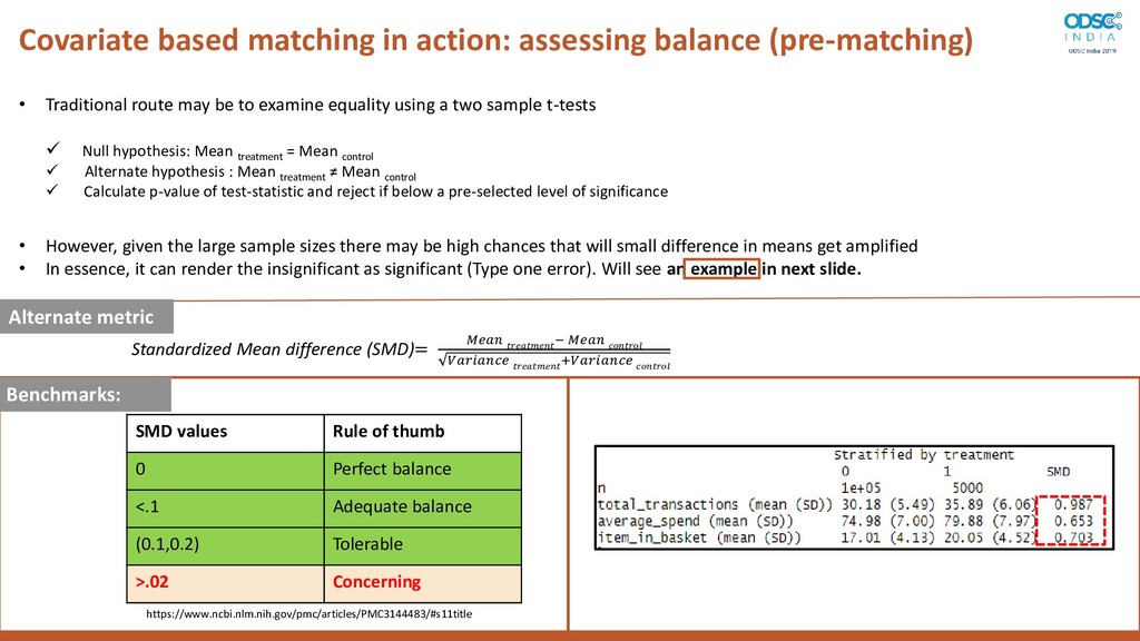
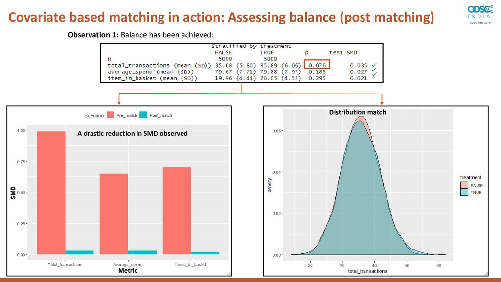
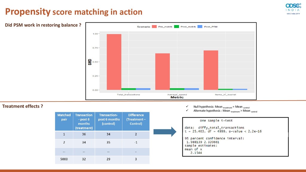
18. Covariate based matching in action: assessing balance (pre-matching) • Traditional route may be to examine equality using a two sample t-tests  Null hypothesis: Mean treatment = Mean control  Alternate hypothesis : Mean treatment ≠ Mean control  Calculate p-value of test-statistic and reject if below a pre-selected level of significance • However, given the large sample sizes there may be high chances that will small difference in means get amplified • In essence, it can render the insignificant as significant (Type one error). Will see an example in next slide. Standardized Mean difference (SMD)= − + Alternate metric SMD values Rule of thumb 0 Perfect balance <.1 Adequate balance (0.1,0.2) Tolerable >.02 Concerning Results from our data: Benchmarks: https://www.ncbi.nlm.nih.gov/pmc/articles/PMC3144483/#s11title
19. Covariate based matching in action: Assessing balance (post matching)  Observation 1: Balance has been achieved:   A drastic reduction in SMD observed Distribution match
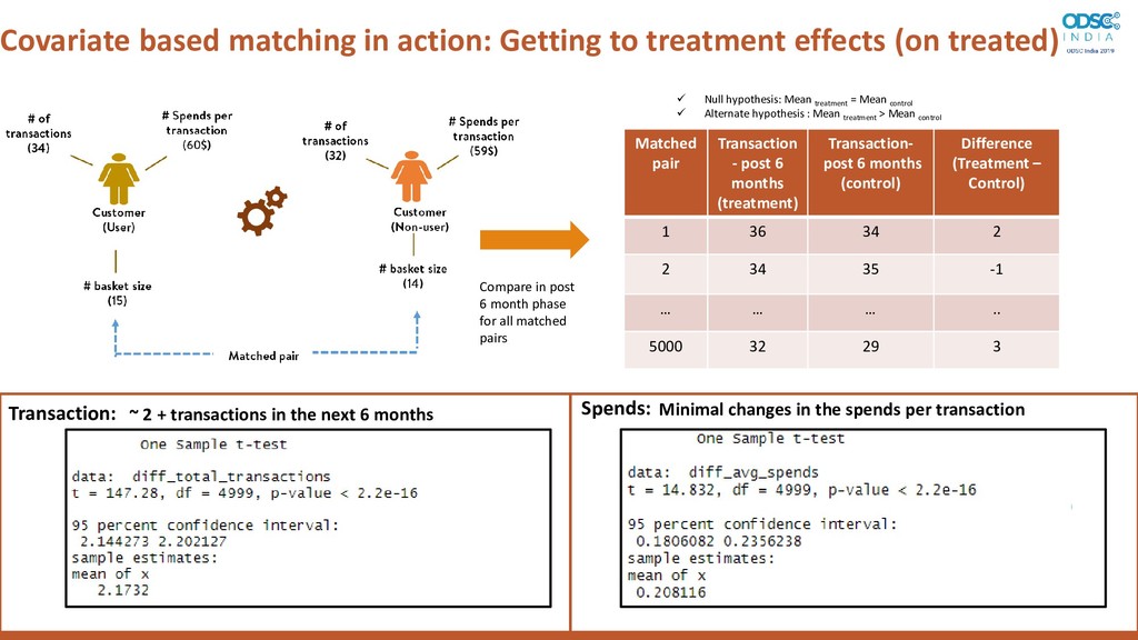
20. Covariate based matching in action: Getting to treatment effects (on treated) Matched pair Transaction - post 6 months (treatment) Transaction- post 6 months (control) Difference (Treatment – Control) 1 36 34 2 2 34 35 -1 … … … .. 5000 32 29 3 Compare in post 6 month phase for all matched pairs  Null hypothesis: Mean treatment = Mean control  Alternate hypothesis : Mean treatment > Mean control Spends: Transaction: ~ 2 + transactions in the next 6 months Minimal changes in the spends per transaction
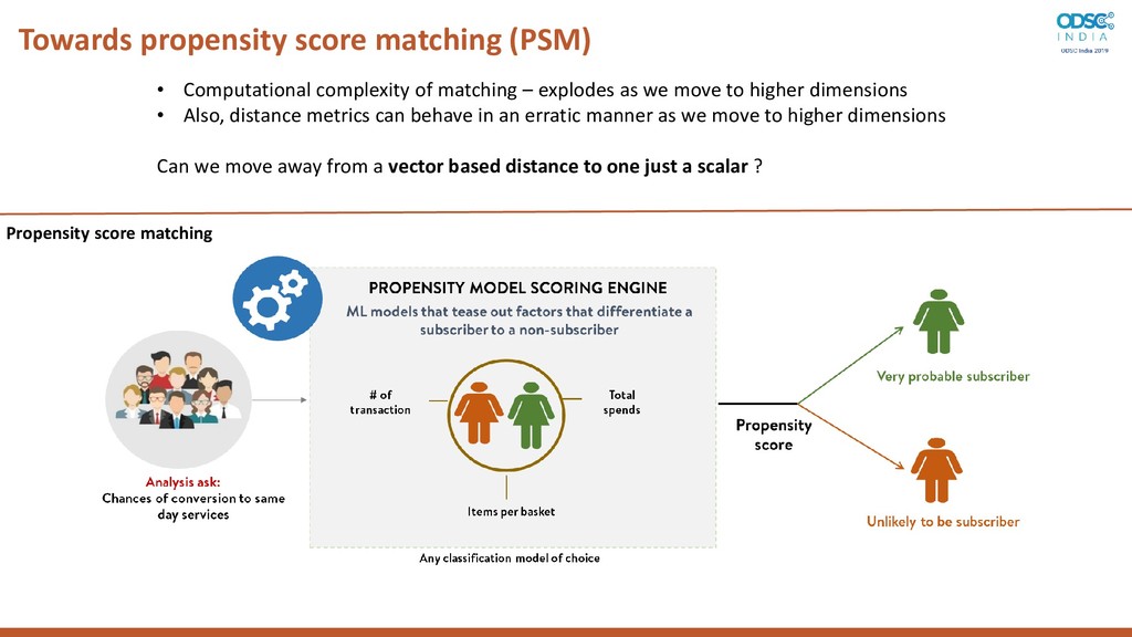
21. Towards propensity score matching (PSM) Propensity score matching • Computational complexity of matching – explodes as we move to higher dimensions • Also, distance metrics can behave in an erratic manner as we move to higher dimensions Can we move away from a vector based distance to one just a scalar ?
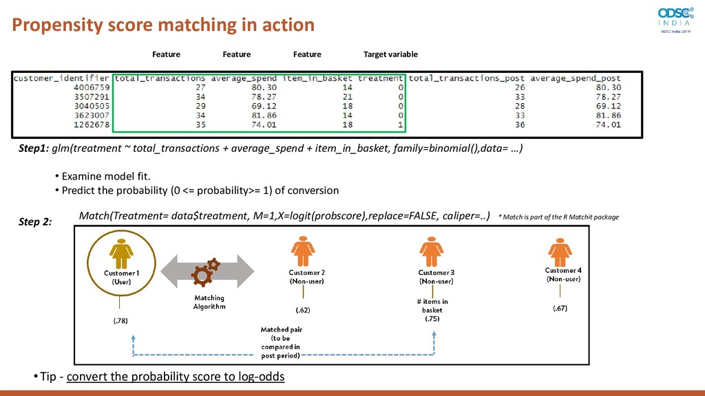
22. Propensity score matching in action Feature Feature Feature Target variable Step1: glm(treatment ~ total_transactions + average_spend + item_in_basket, family=binomial(),data= …) • Examine model fit. • Predict the probability (0 <= probability>= 1) of conversion Step 2: Match(Treatment= data$treatment, M=1,X=logit(probscore),replace=FALSE, caliper=..) * Match is part of the R Matchit package • Tip - convert the probability score to log-odds
23. Propensity score matching in action Did PSM work in restoring balance ? Treatment effects ?  Null hypothesis: Mean treatment = Mean control  Alternate hypothesis : Mean treatment > Mean control
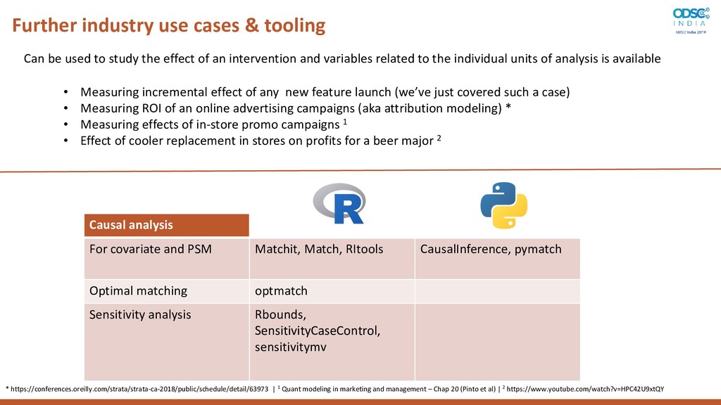
24. Further industry use cases & tooling Causal analysis R packages Python packages For covariate and PSM Matchit, Match, RItools CausalInference, pymatch Optimal matching optmatch Sensitivity analysis Rbounds, SensitivityCaseControl, sensitivitymv Can be used to study the effect of an intervention and variables related to the individual units of analysis is available • Measuring incremental effect of any new feature launch (we’ve just covered such a case) • Measuring ROI of an online advertising campaigns (aka attribution modeling) * • Measuring effects of in-store promo campaigns 1 • Effect of cooler replacement in stores on profits for a beer major 2 * https://conferences.oreilly.com/strata/strata-ca-2018/public/schedule/detail/63973 | 1 Quant modeling in marketing and management – Chap 20 (Pinto et al) | 2 https://www.youtube.com/watch?v=HPC42U9xtQY
25. There’s much more to matching methods ! GitHub repository for this talk: https://github.com/subhasishmisra/causal_data_science
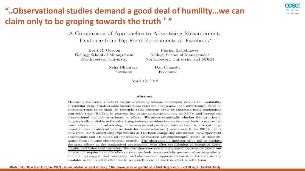
26. “..Observational studies demand a good deal of humility…we can claim only to be groping towards the truth * ” * Attributed to Dr William Cochran (1972) – Journal of observational studies | * The shown paper was published in Marketing Science – Vol 38, No 2 . Available freely.
27. New directions – the promise of ML https://www.datasciencecentral.com/profiles/blogs/causality-the-next-most-important-thing-in-ai-ml https://www.technologyreview.com/s/613502/deep-learning-could-reveal-why-the-world-works-the-way-it-does/ https://www.quantamagazine.org/to-build-truly-intelligent-machines-teach-them-cause-and-effect-20180515/ https://www.bu.edu/cphs/files/2013/01/Mark-van-der-Laan-Targeted-Learning-with-Big-Data.pdf https://www.goodreads.com/book/show/36204378-the-book-of-why
28. For questions, please contact: Subhasish Misra E-mail: misrasubhasish@gmail.com/subhasish.misra@walmart.com LinkedIn: https://www.linkedin.com/in/subhasish-misra-5885995/ 28 Thank you for your time !