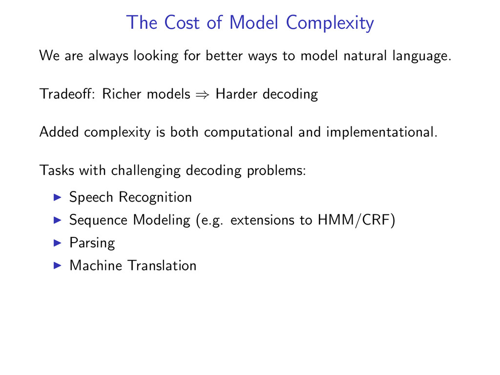
better ways to model natural language. Tradeoff: Richer models ⇒ Harder decoding Added complexity is both computational and implementational. Tasks with challenging decoding problems: Speech Recognition Sequence Modeling (e.g. extensions to HMM/CRF) Parsing Machine Translation
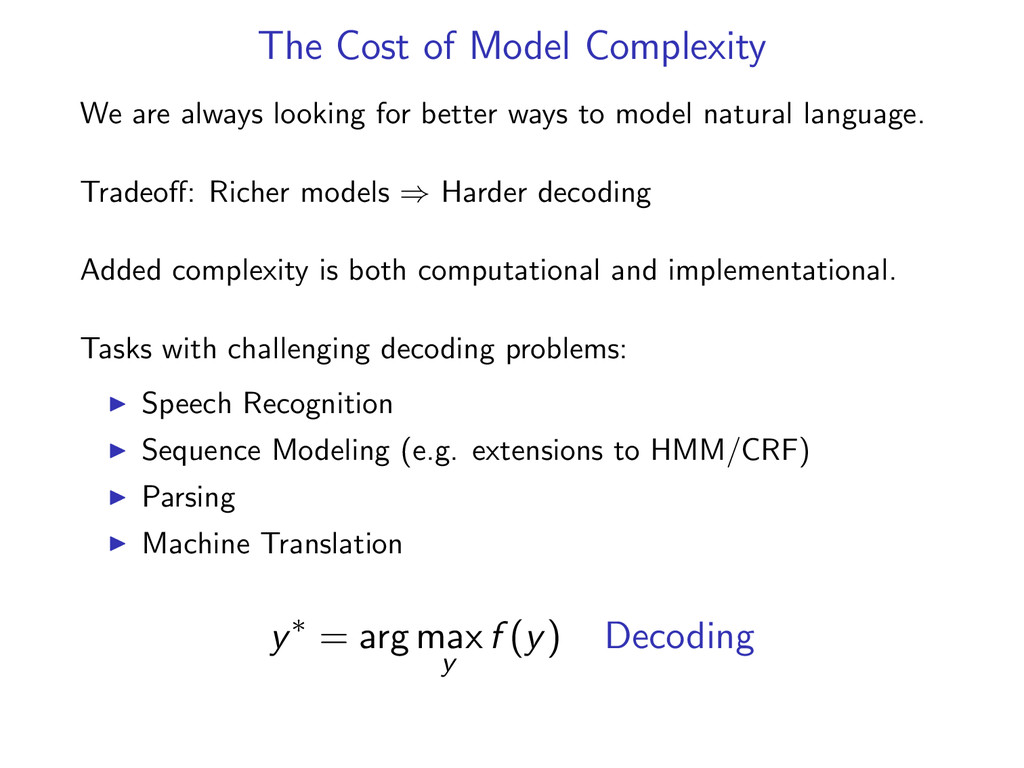
better ways to model natural language. Tradeoff: Richer models ⇒ Harder decoding Added complexity is both computational and implementational. Tasks with challenging decoding problems: Speech Recognition Sequence Modeling (e.g. extensions to HMM/CRF) Parsing Machine Translation y∗ = arg max y f (y) Decoding
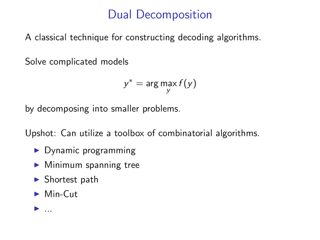
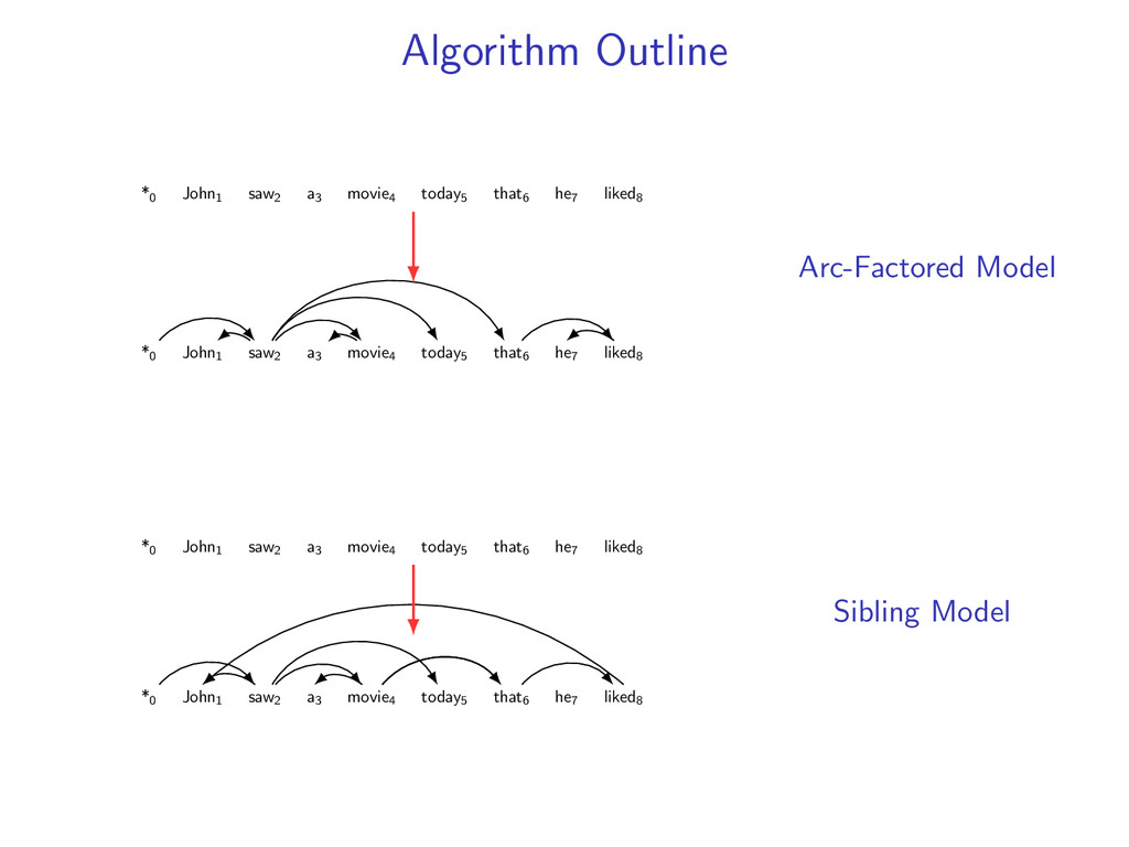
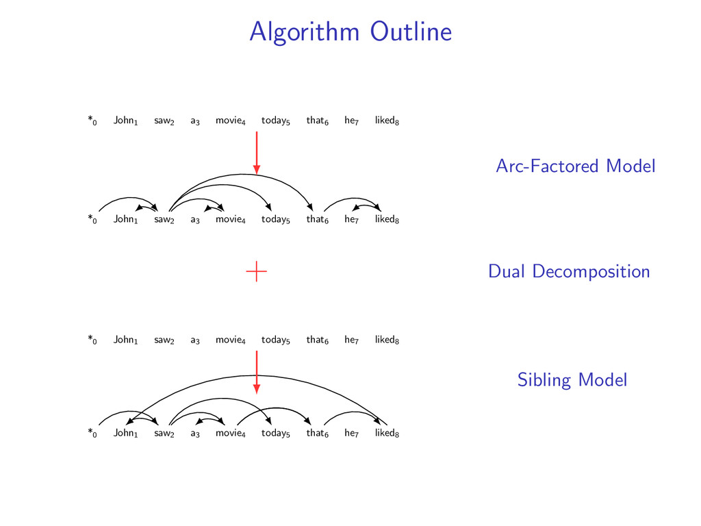
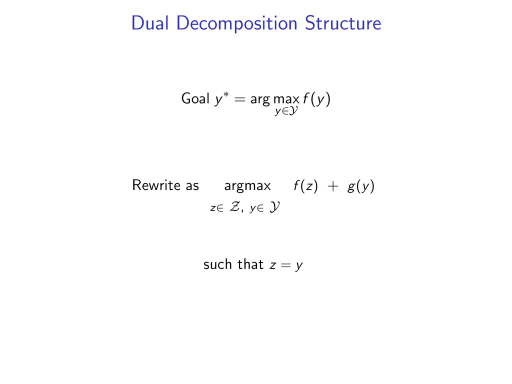
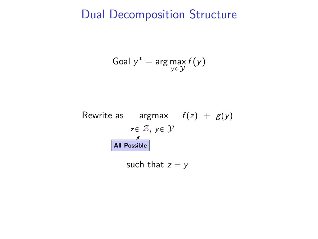
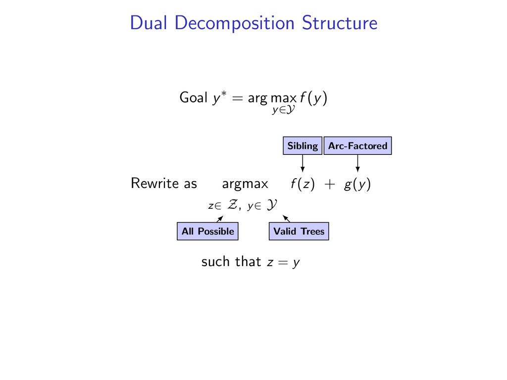
complicated models y∗ = arg max y f (y) by decomposing into smaller problems. Upshot: Can utilize a toolbox of combinatorial algorithms. Dynamic programming Minimum spanning tree Shortest path Min-Cut ...
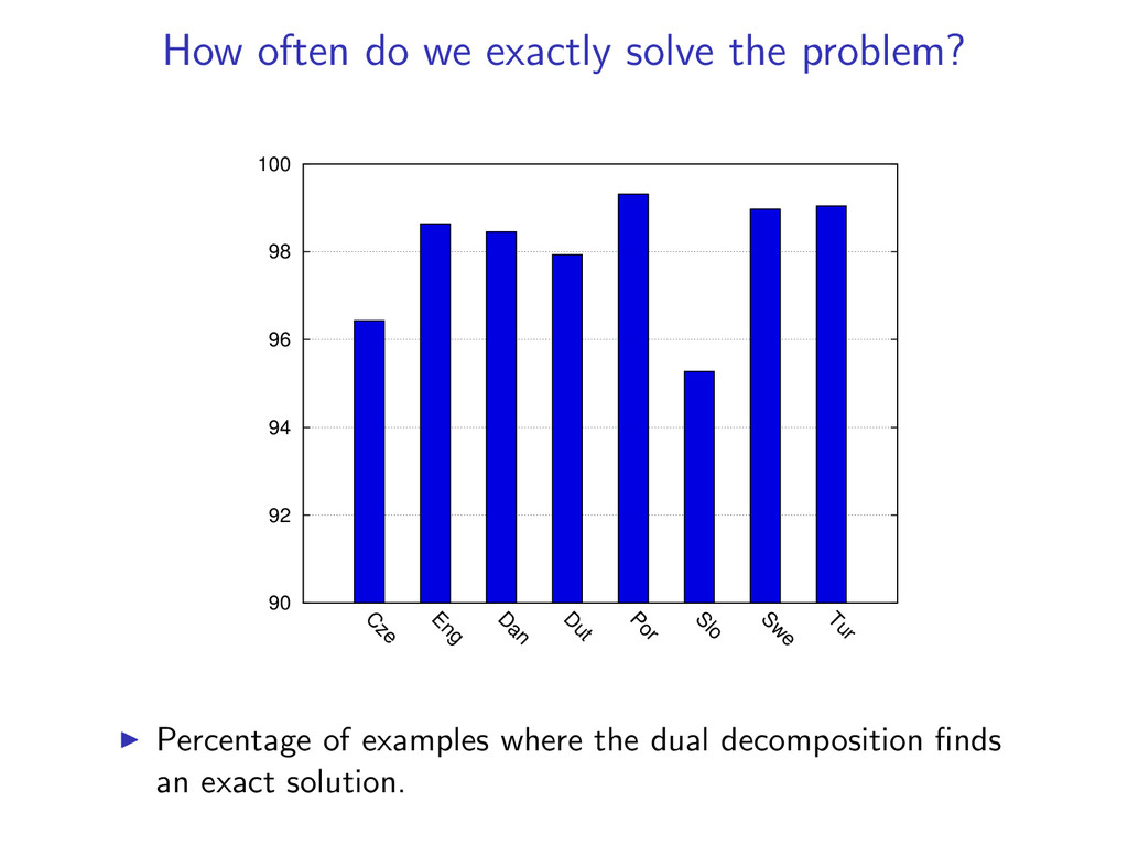
Uses basic combinatorial algorithms Efficient - Faster than previously proposed algorithms Strong Guarantees - Gives a certificate of optimality when exact Solves 98% of examples exactly, even though the problem is NP-Hard Widely Applicable - Similar techniques extend to other problems
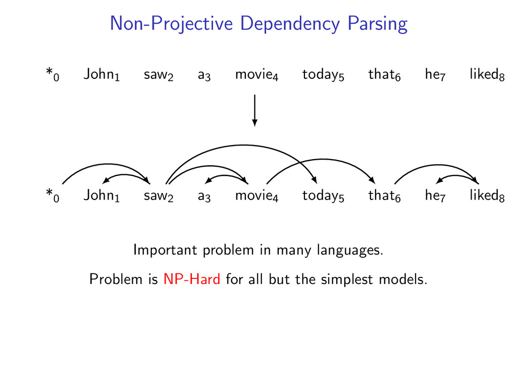
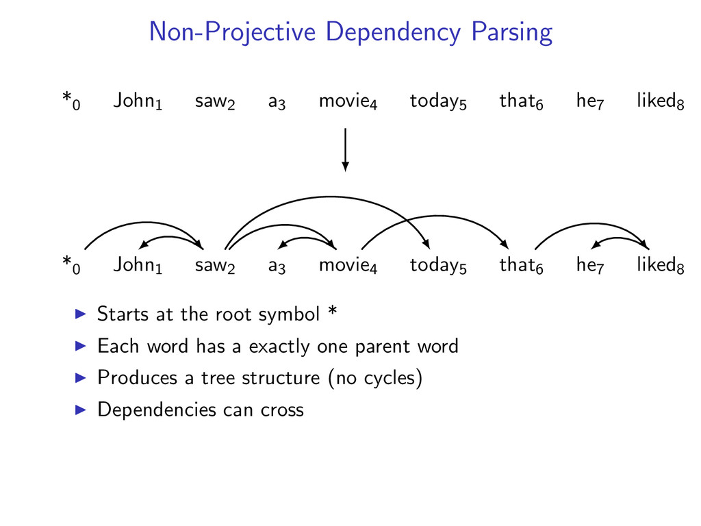
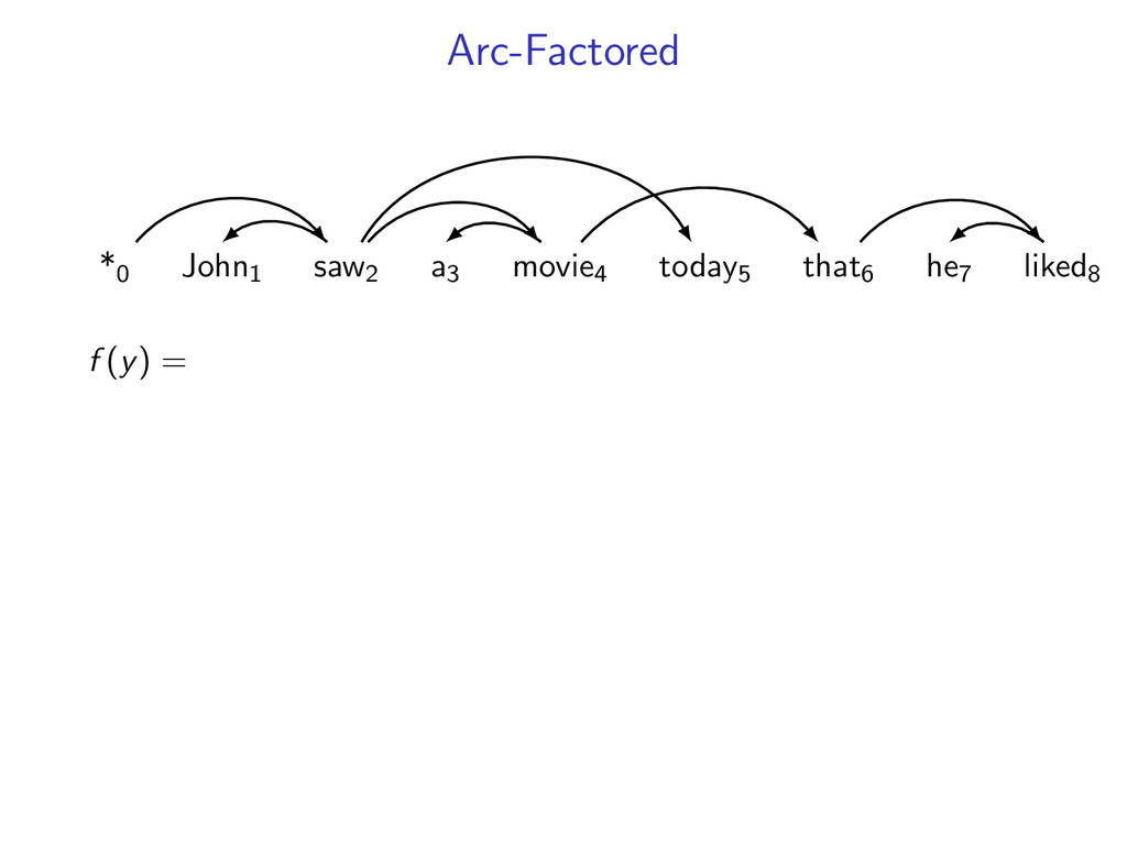
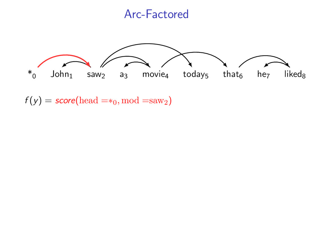
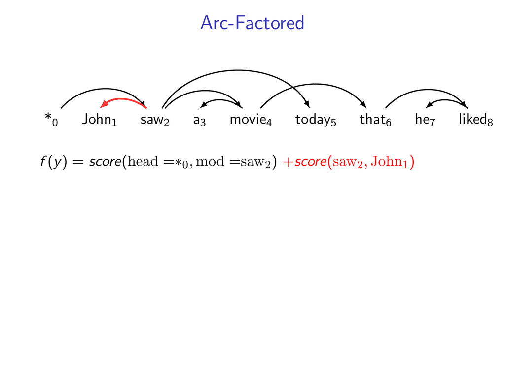
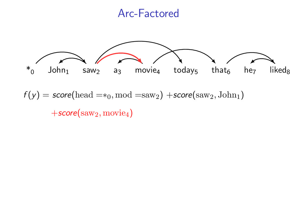
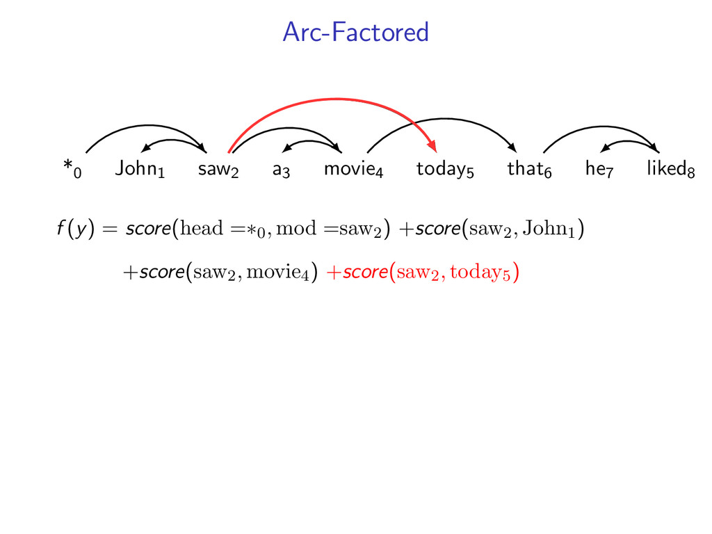
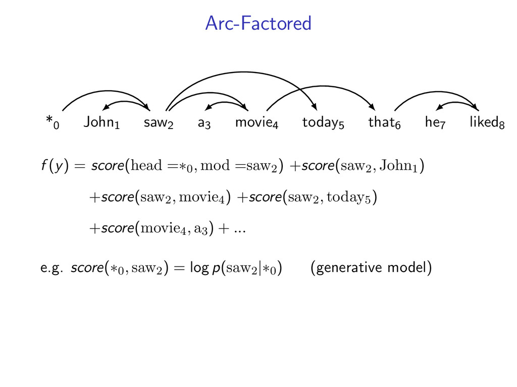
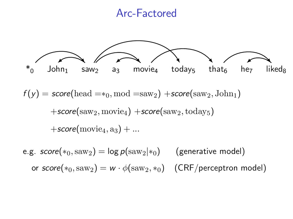
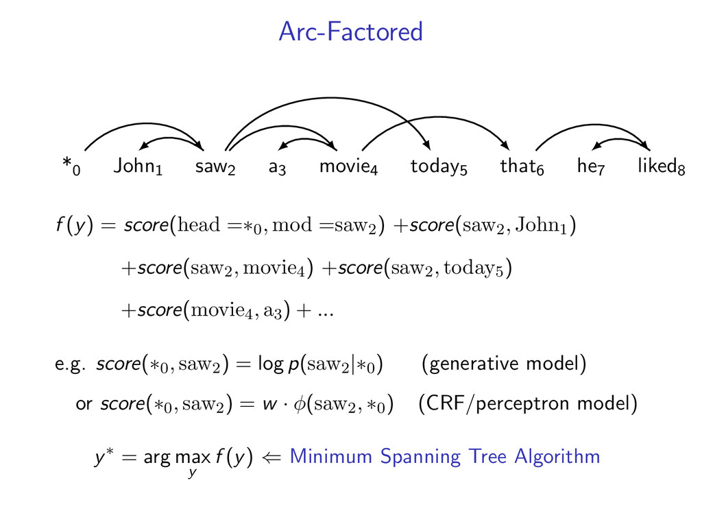
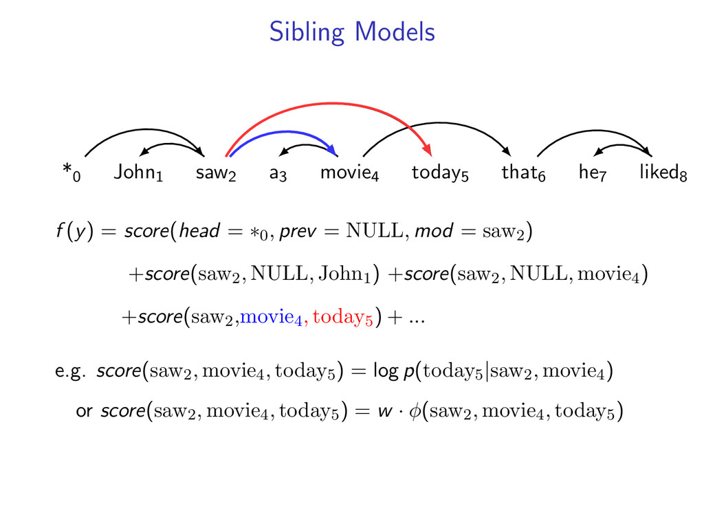
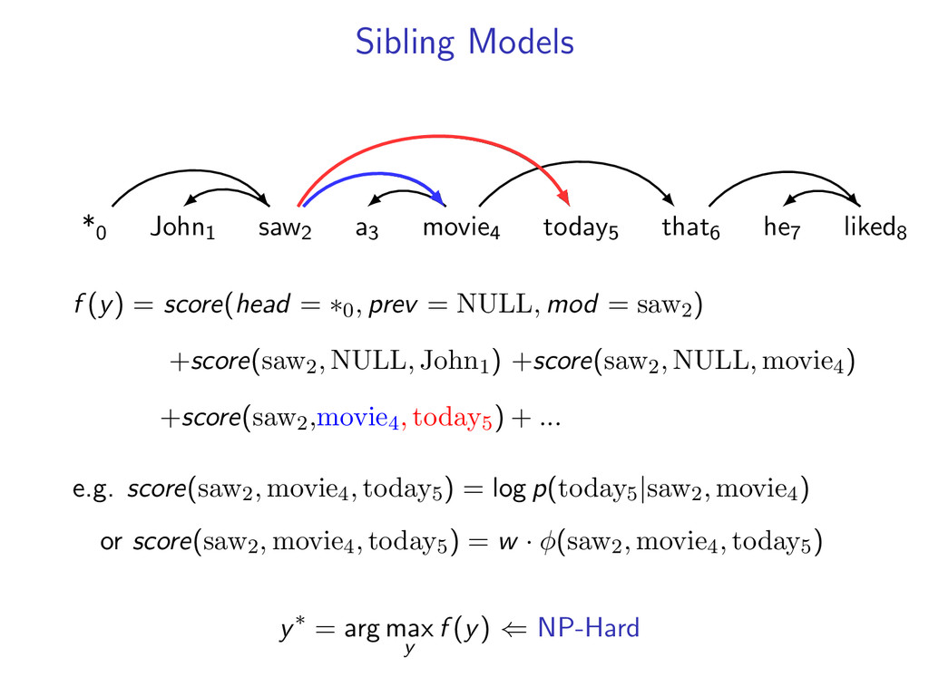
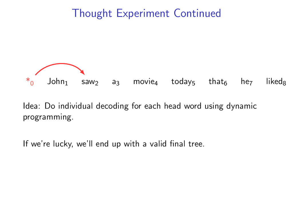
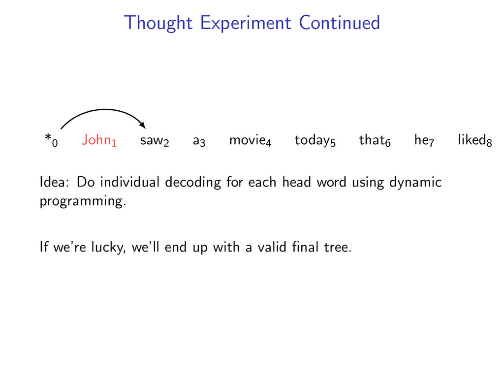
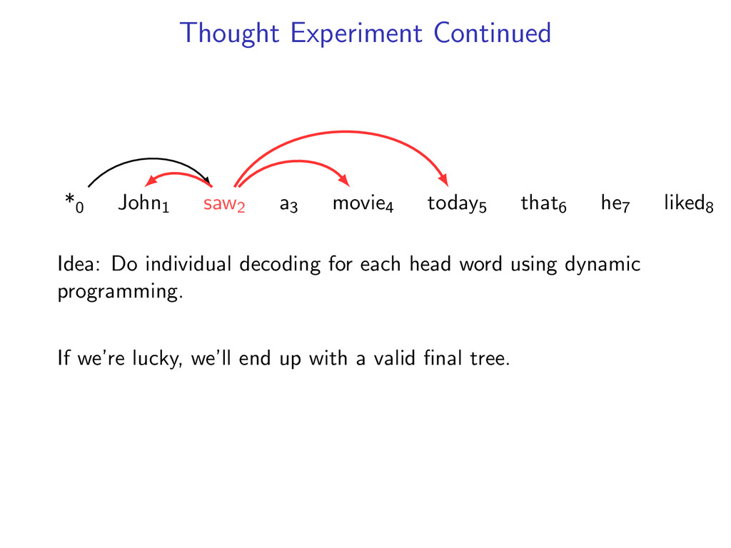
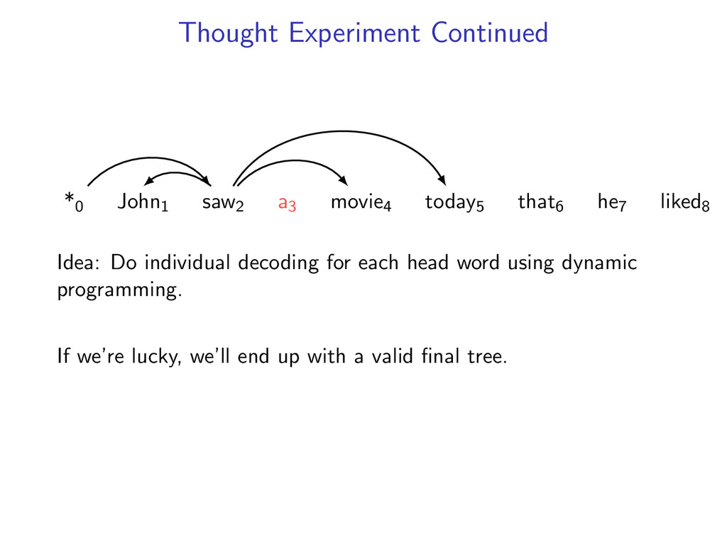
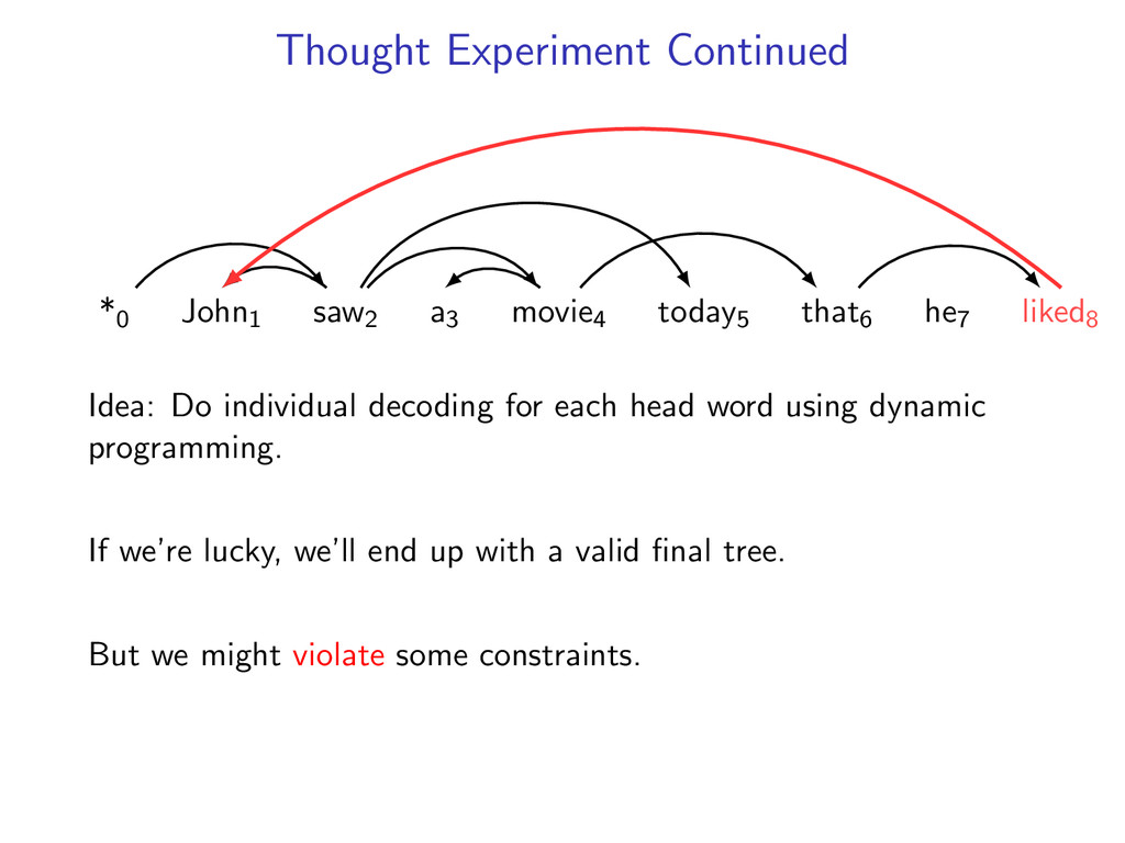
he7 liked8 *0 John1 saw2 a3 movie4 today5 that6 he7 liked8 Starts at the root symbol * Each word has a exactly one parent word Produces a tree structure (no cycles) Dependencies can cross
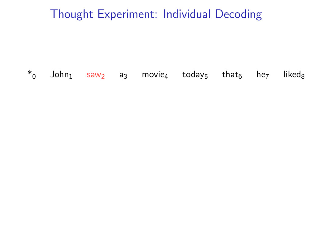
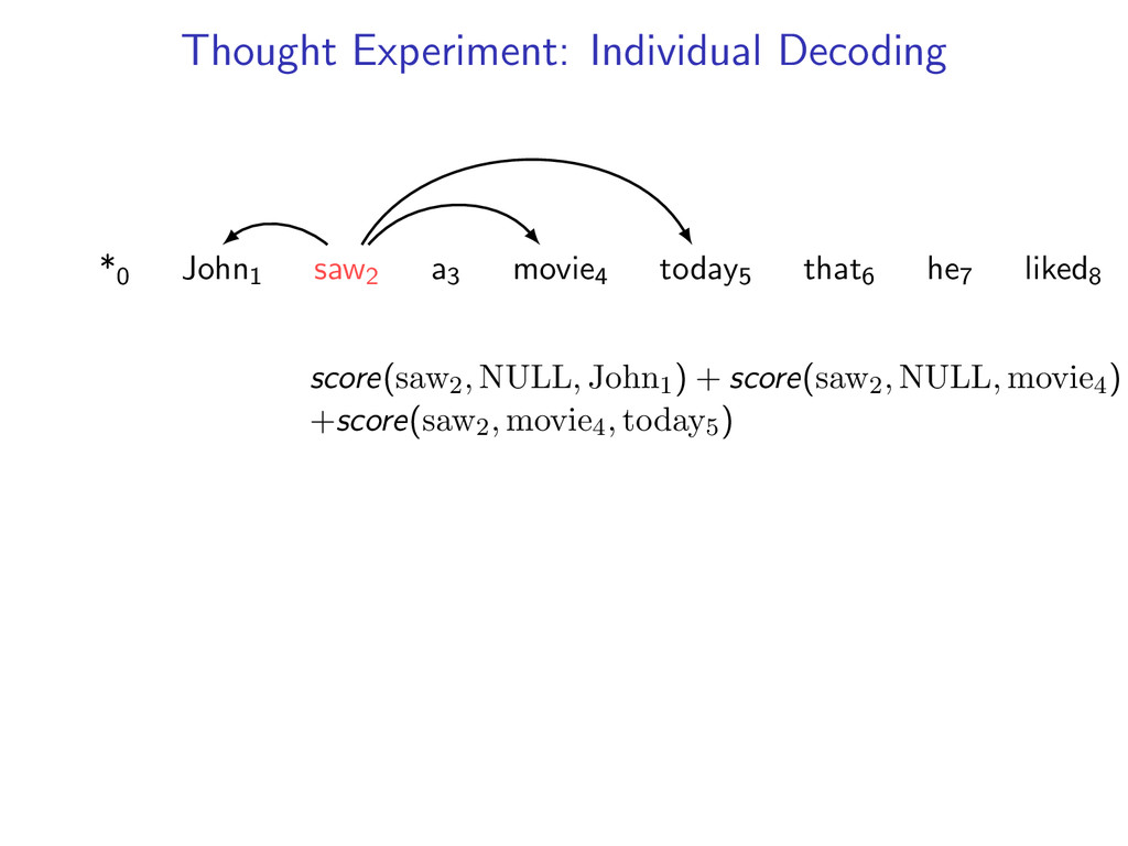
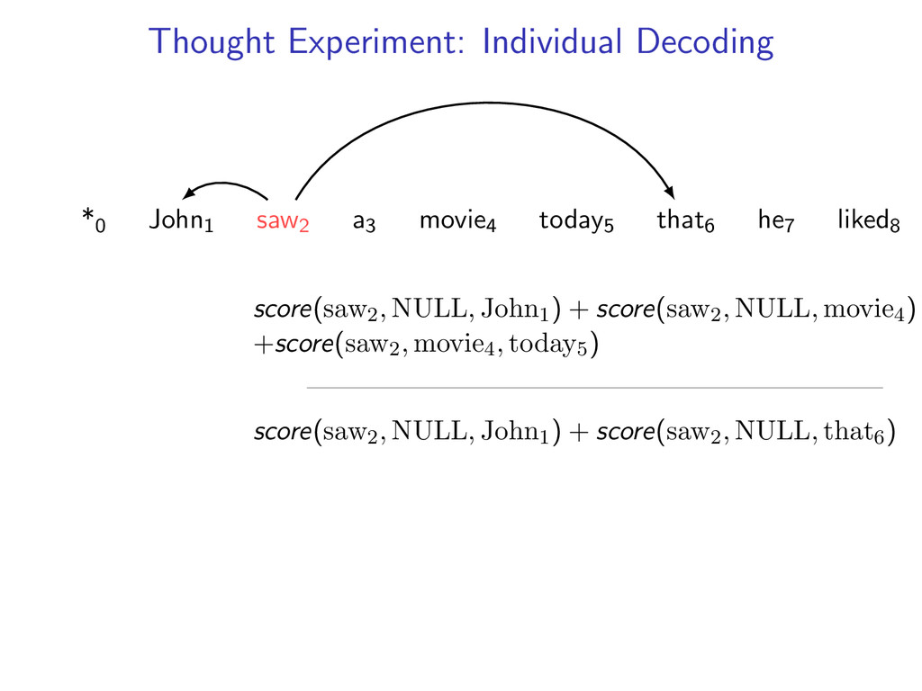
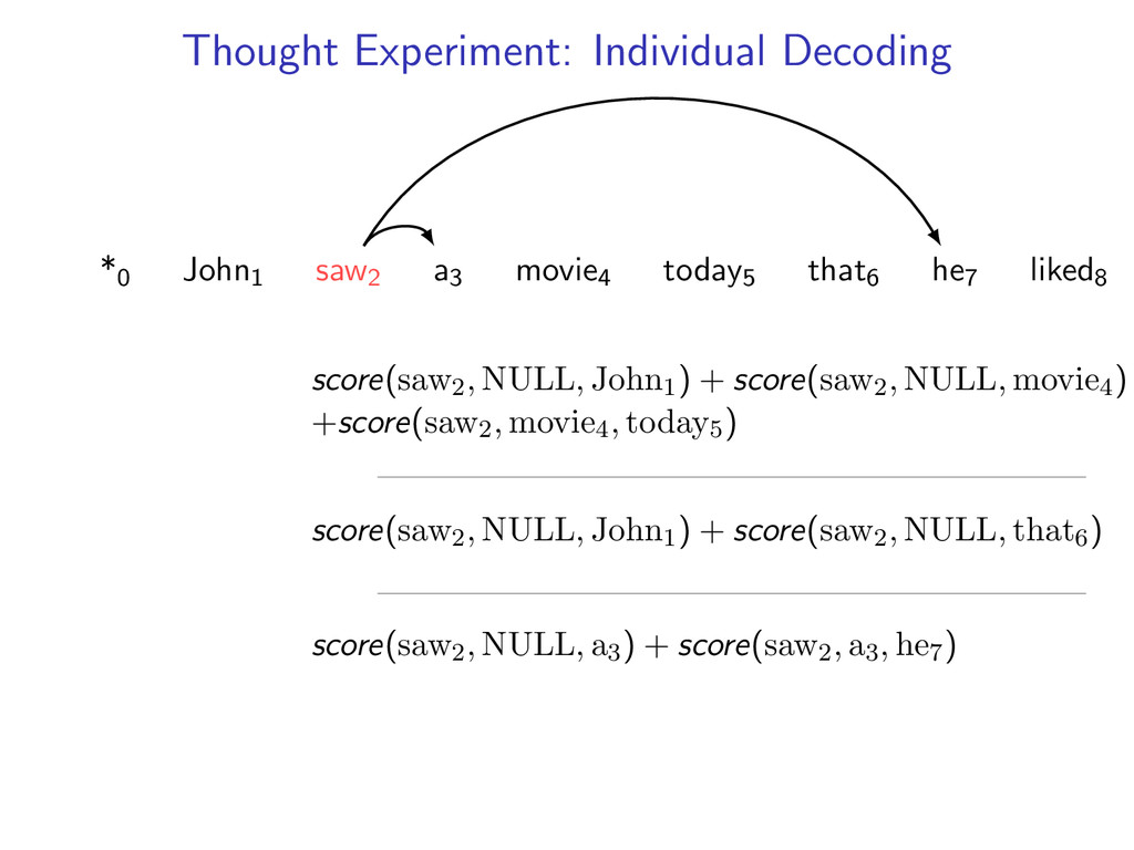
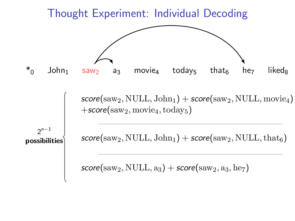
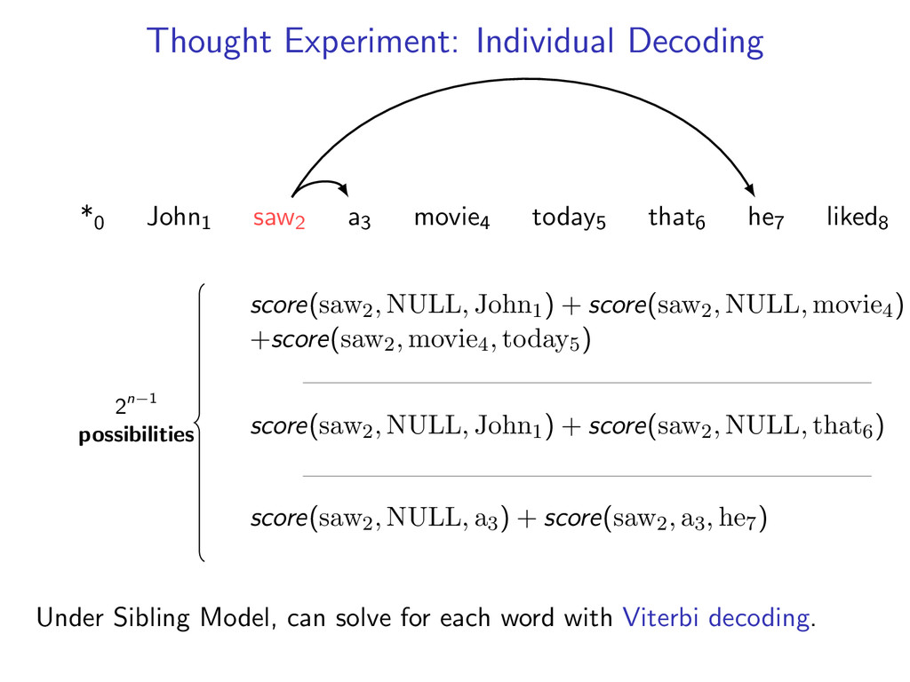
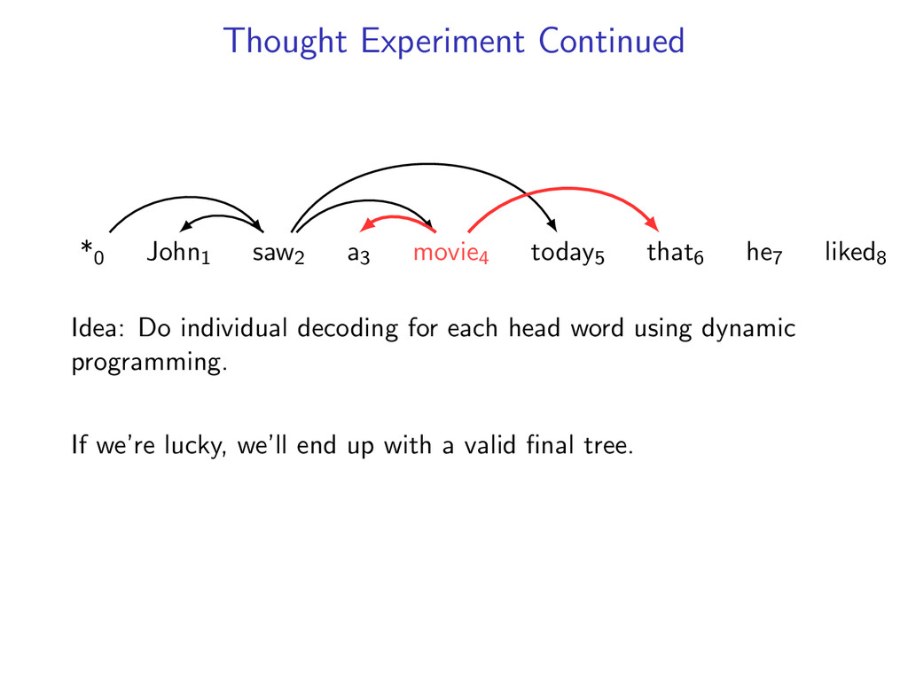
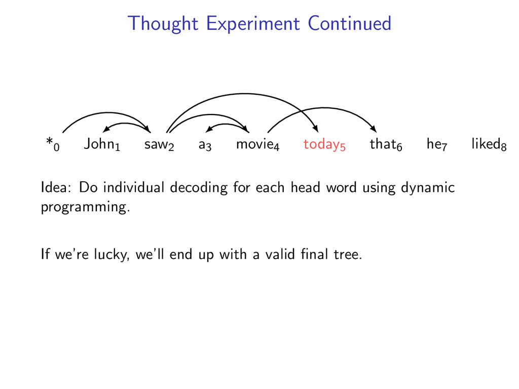
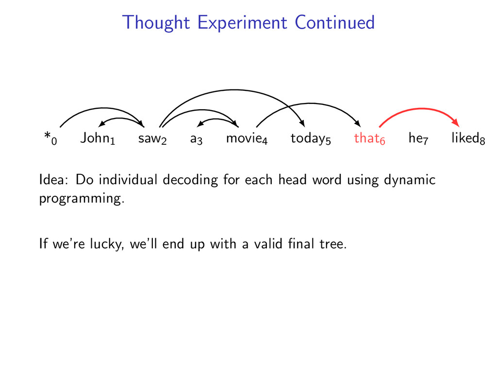
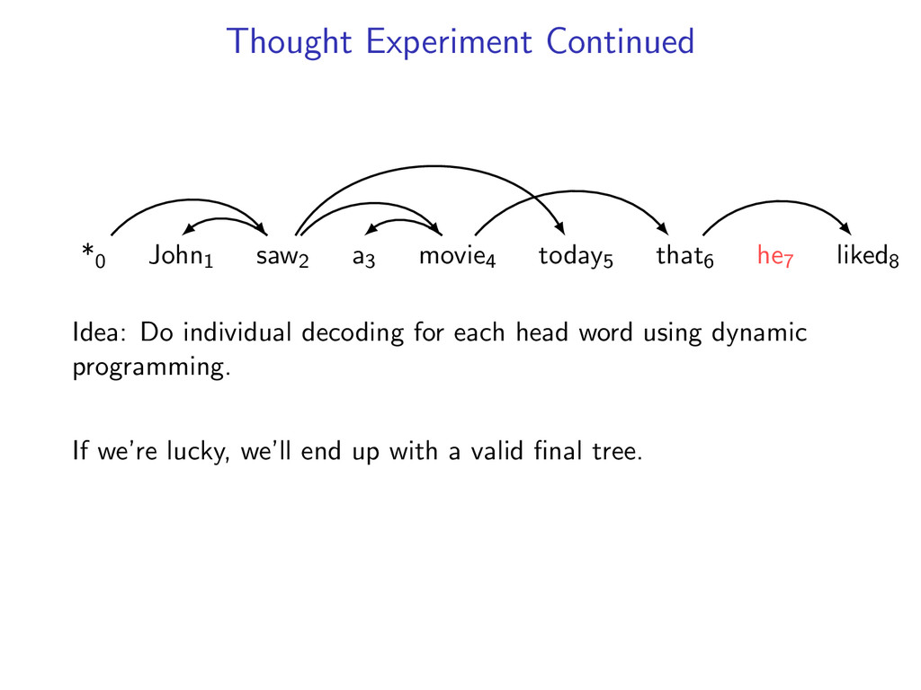
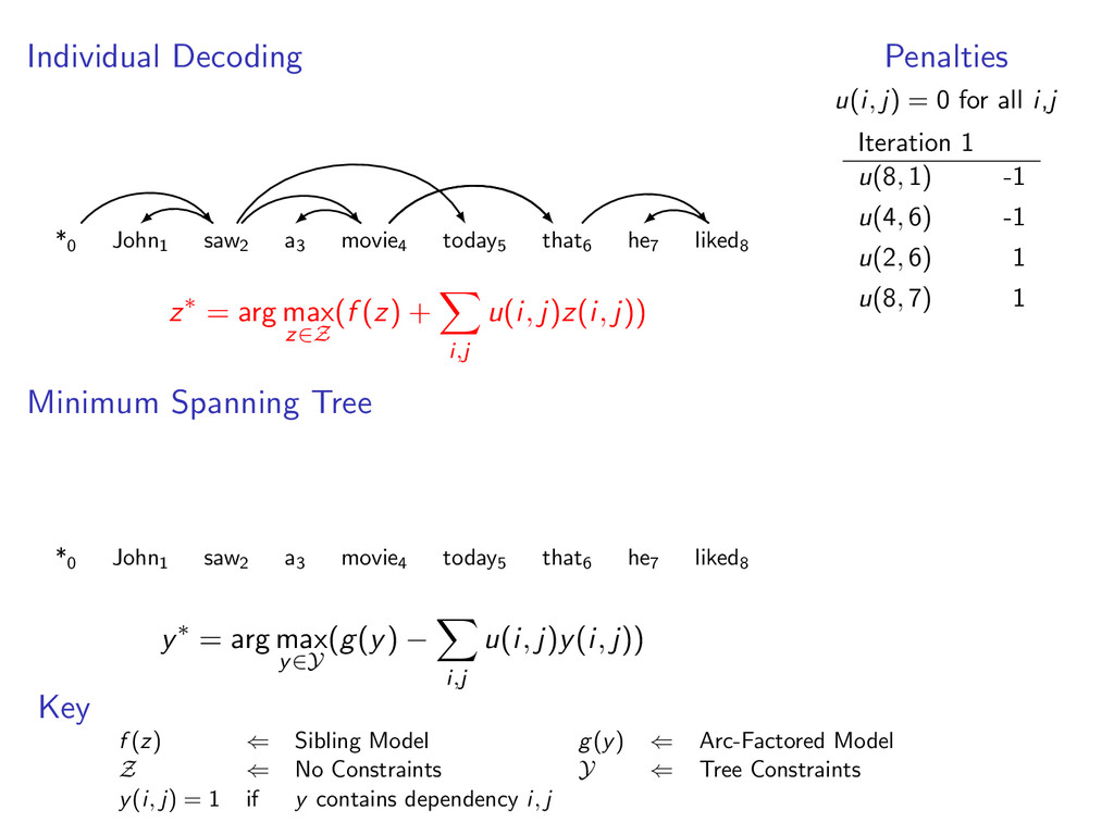
he7 liked8 Idea: Do individual decoding for each head word using dynamic programming. If we’re lucky, we’ll end up with a valid final tree. But we might violate some constraints.
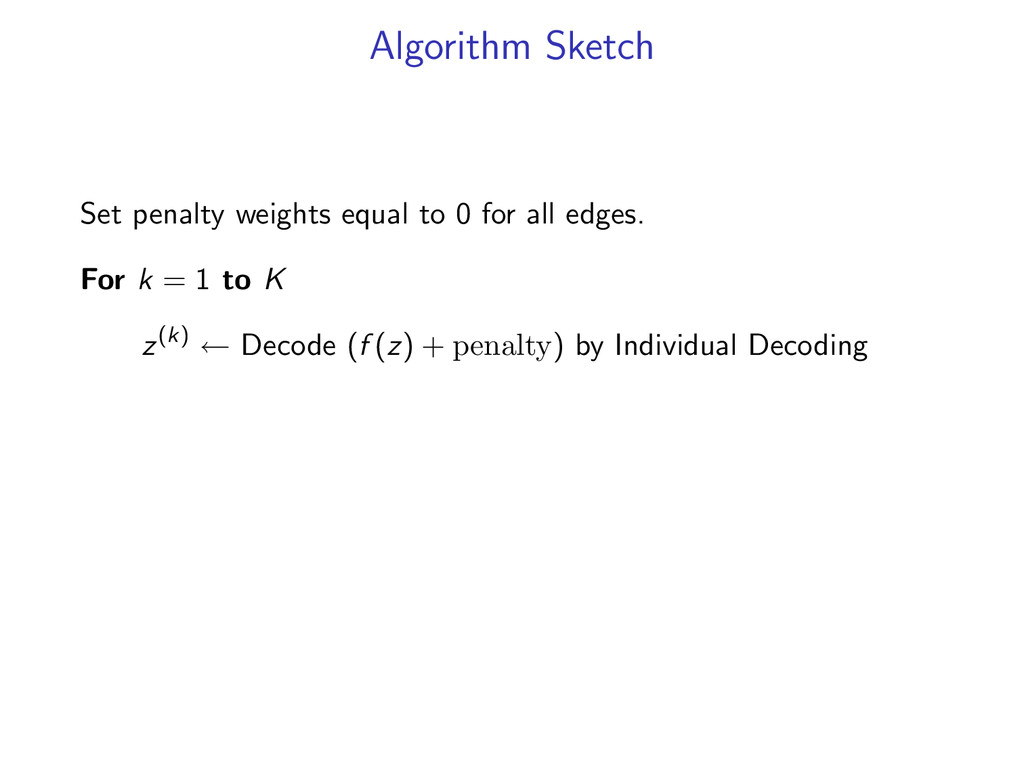
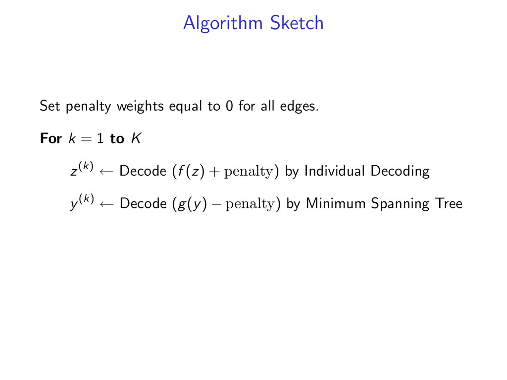
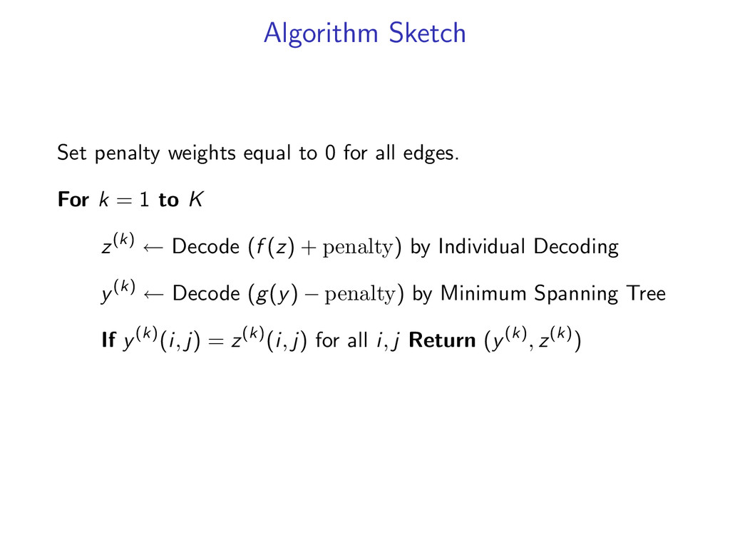
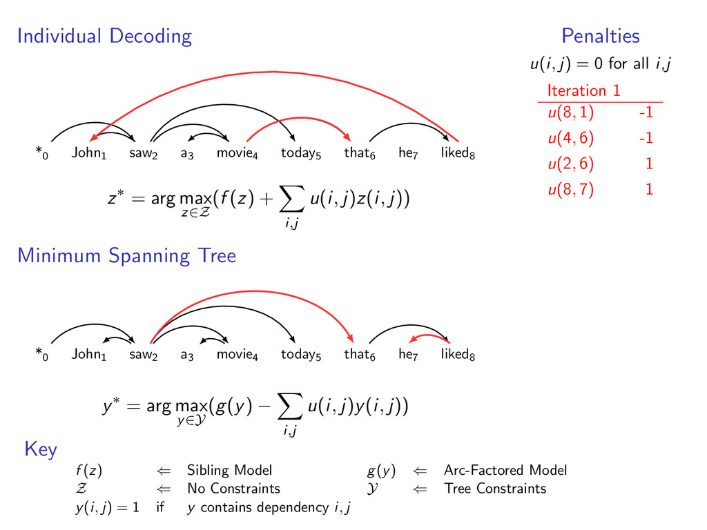
edges. For k = 1 to K z(k) ← Decode (f (z) + penalty) by Individual Decoding y(k) ← Decode (g(y) − penalty) by Minimum Spanning Tree If y(k)(i, j) = z(k)(i, j) for all i, j Return (y(k), z(k))
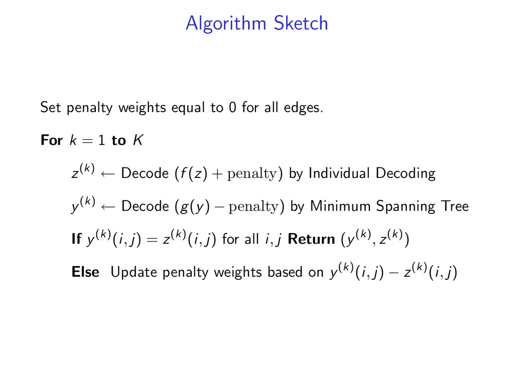
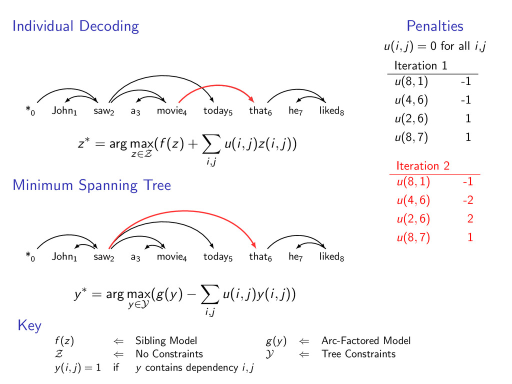
edges. For k = 1 to K z(k) ← Decode (f (z) + penalty) by Individual Decoding y(k) ← Decode (g(y) − penalty) by Minimum Spanning Tree If y(k)(i, j) = z(k)(i, j) for all i, j Return (y(k), z(k)) Else Update penalty weights based on y(k)(i, j) − z(k)(i, j)
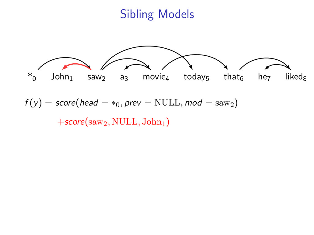
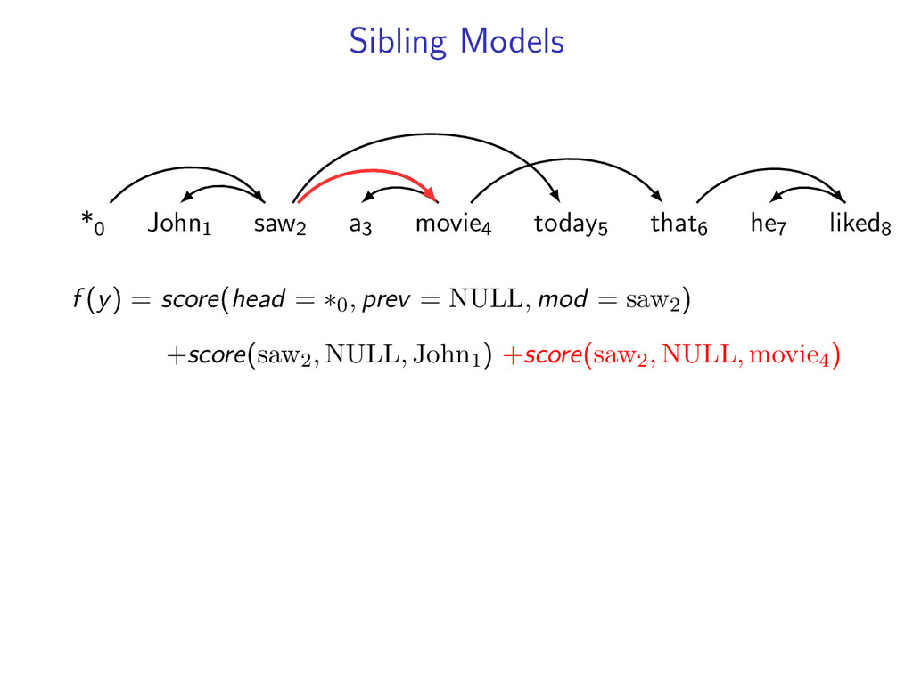
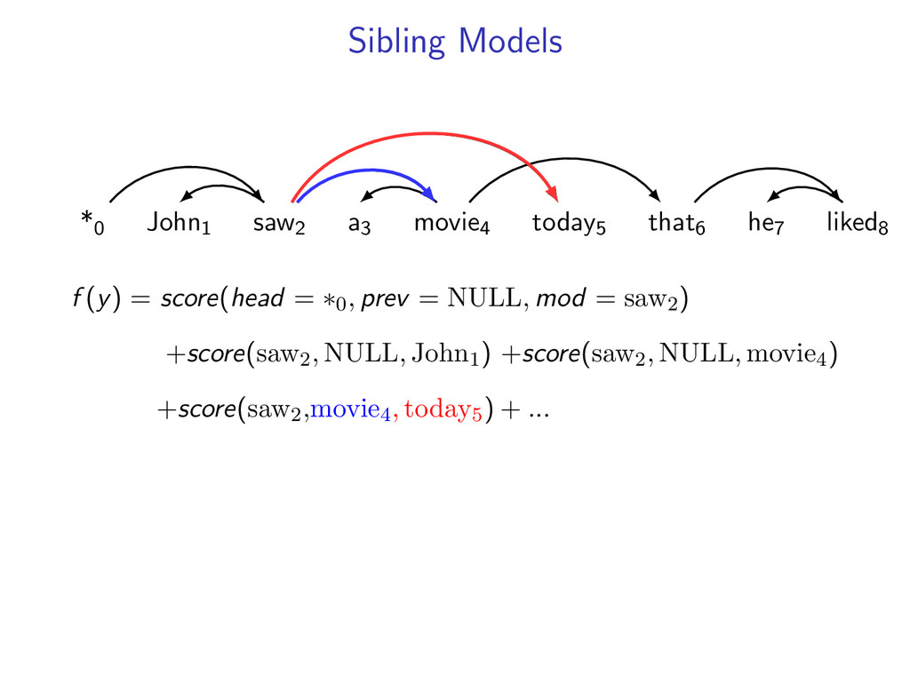
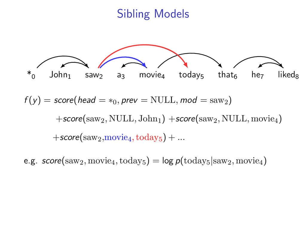
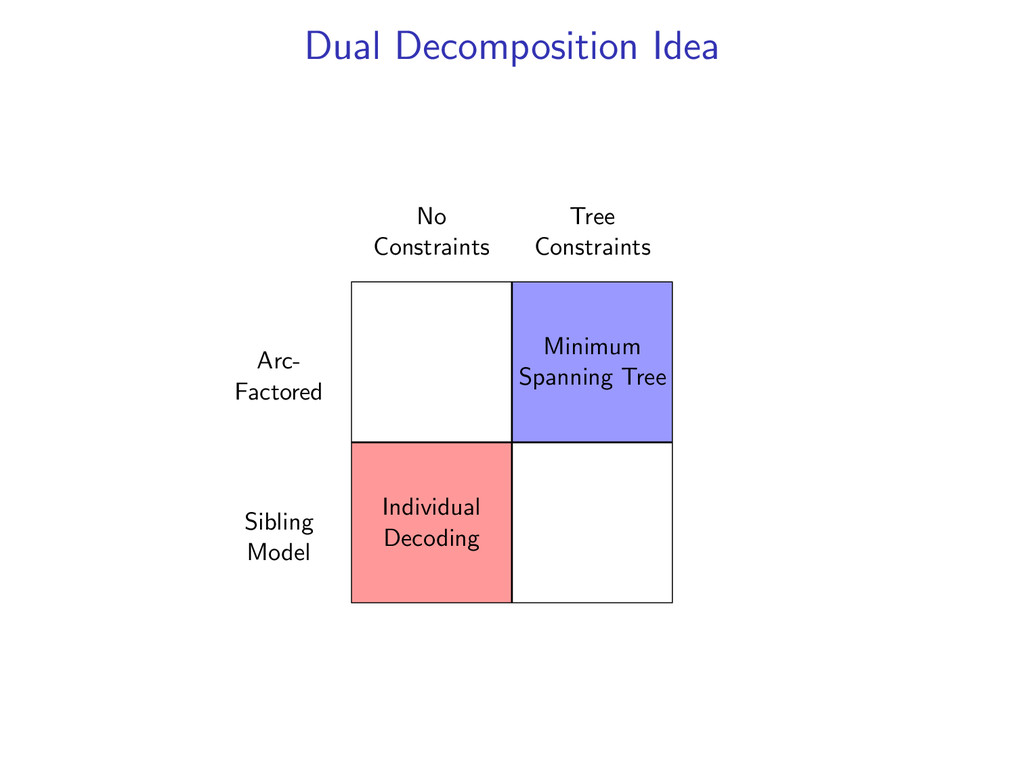
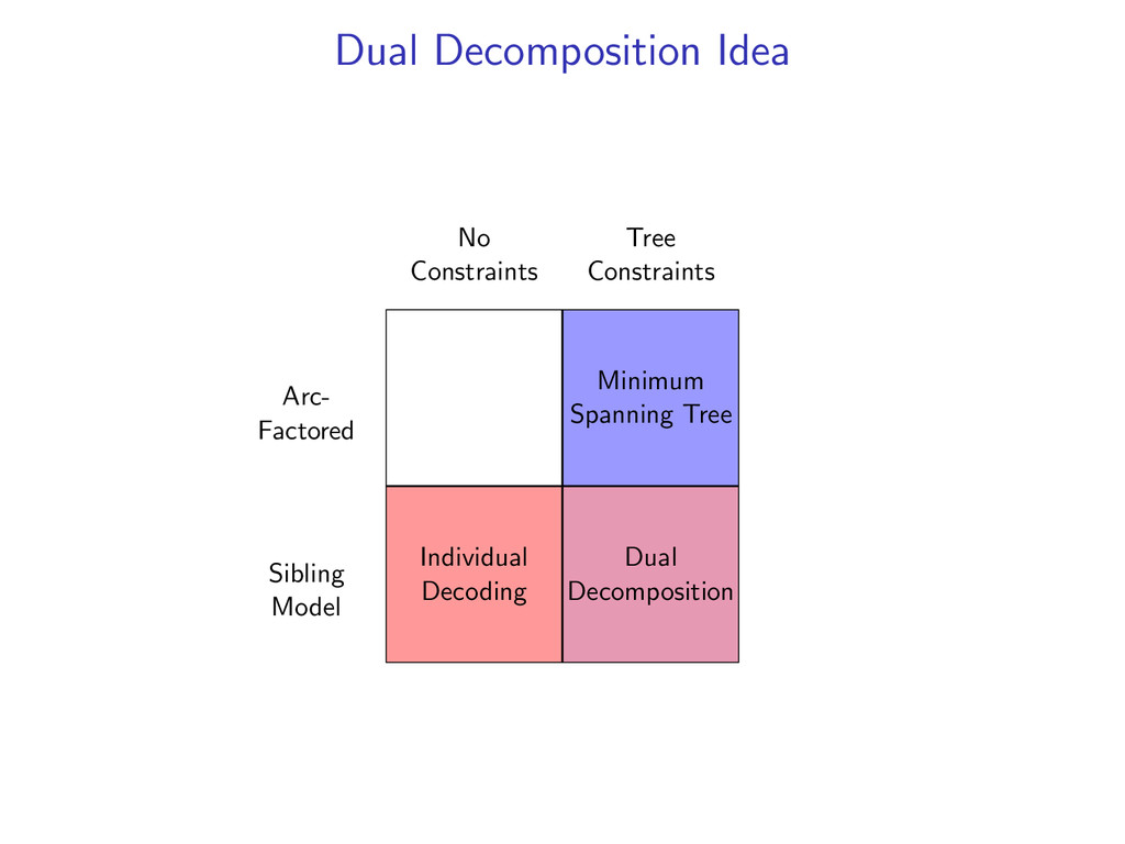
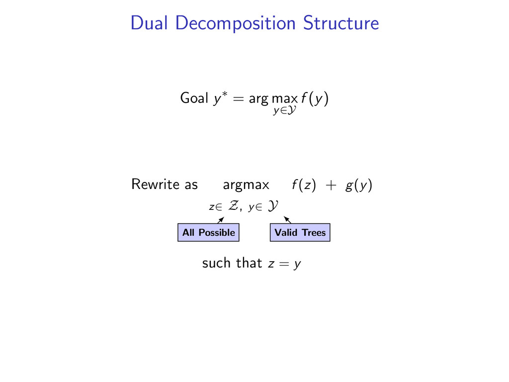
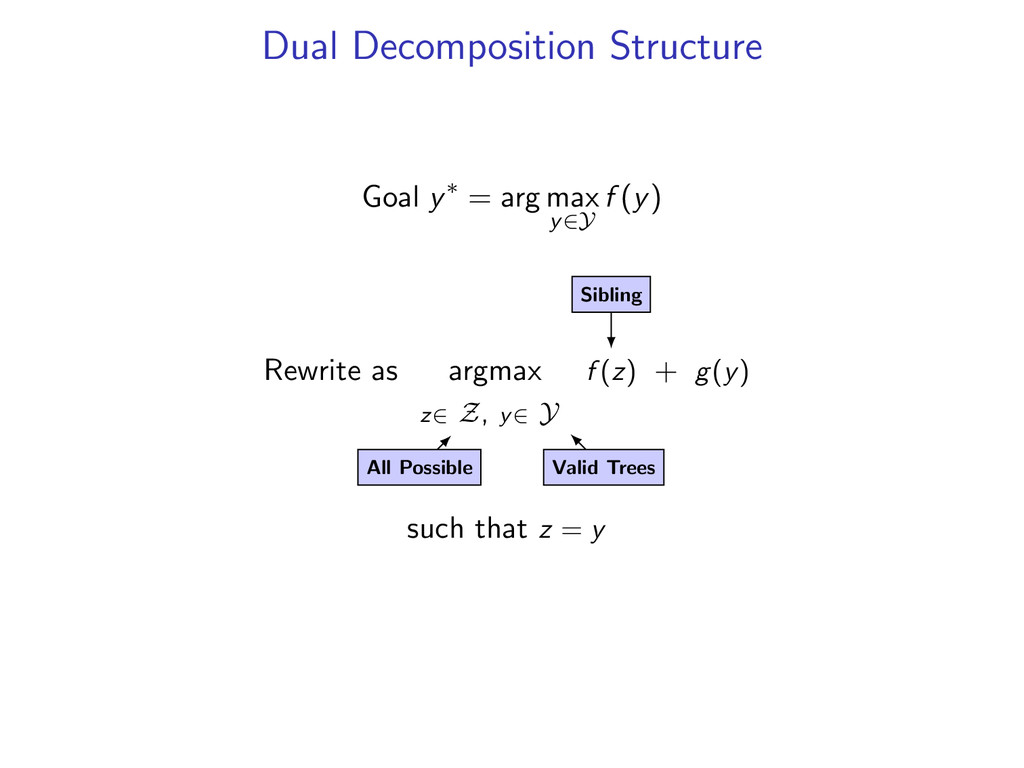
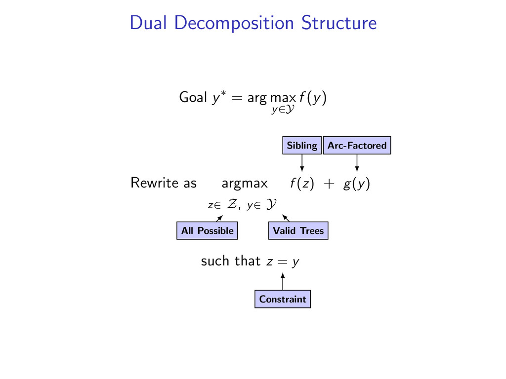
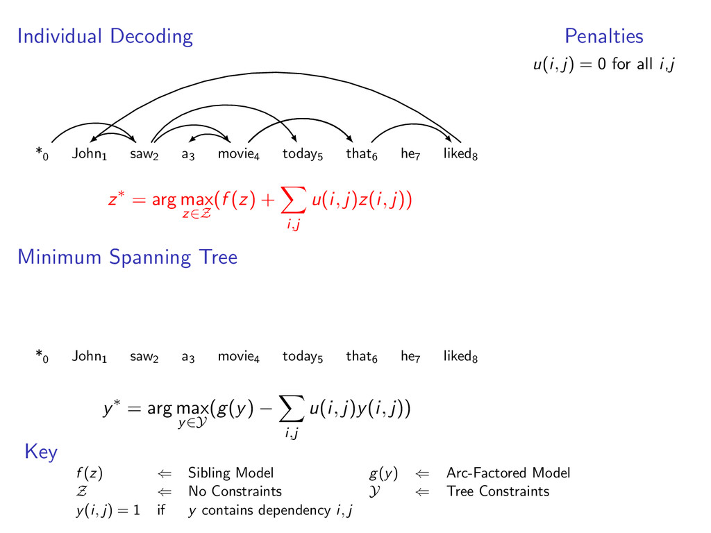
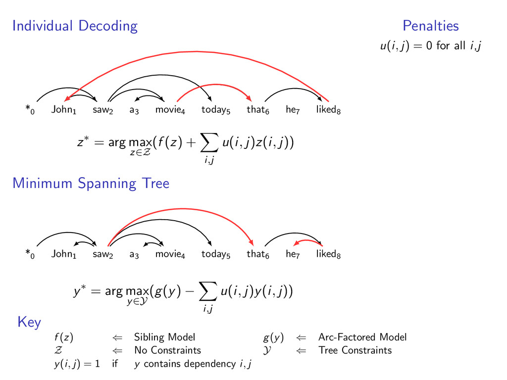
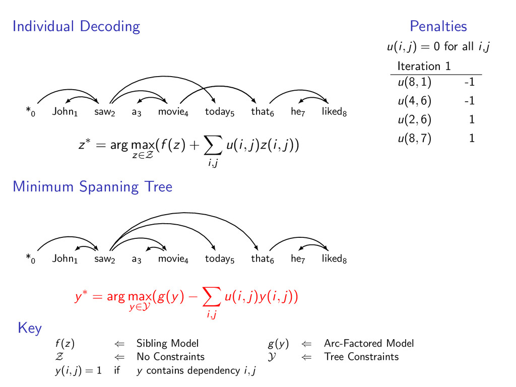
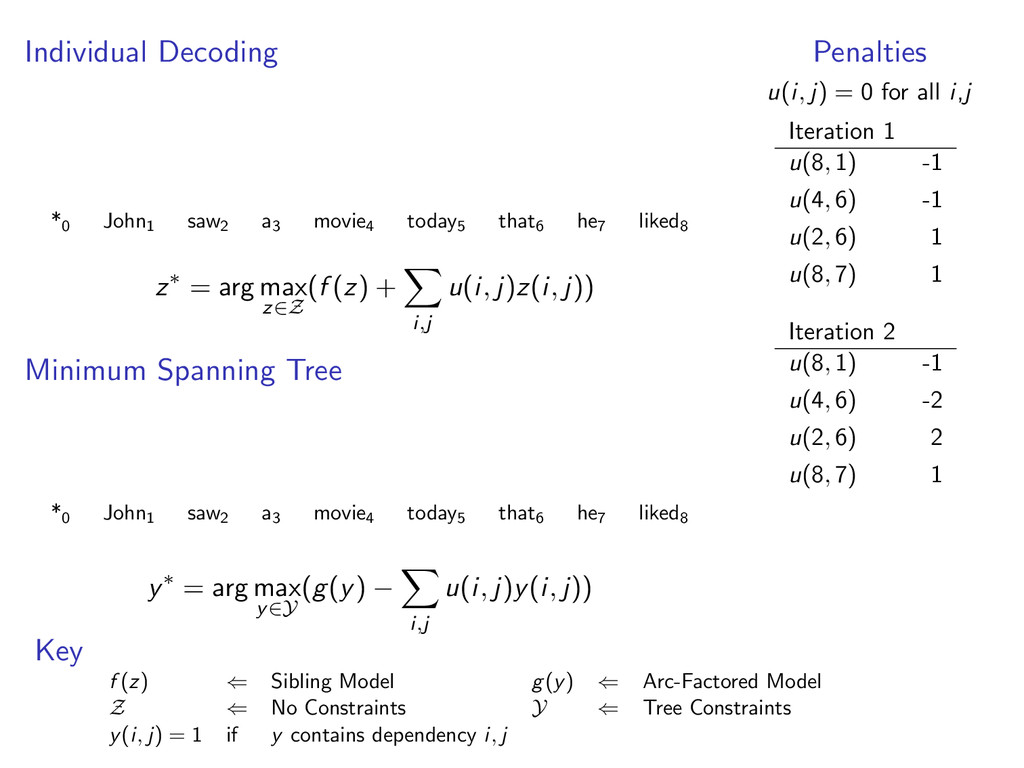
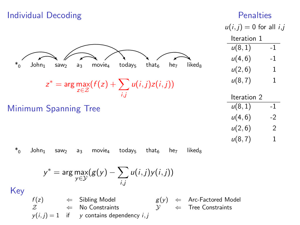
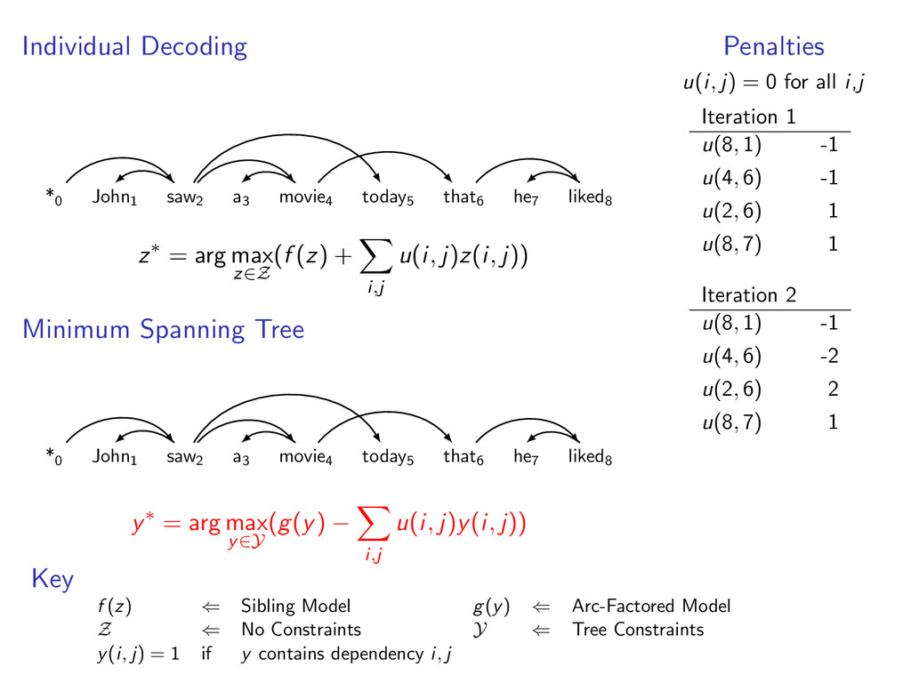
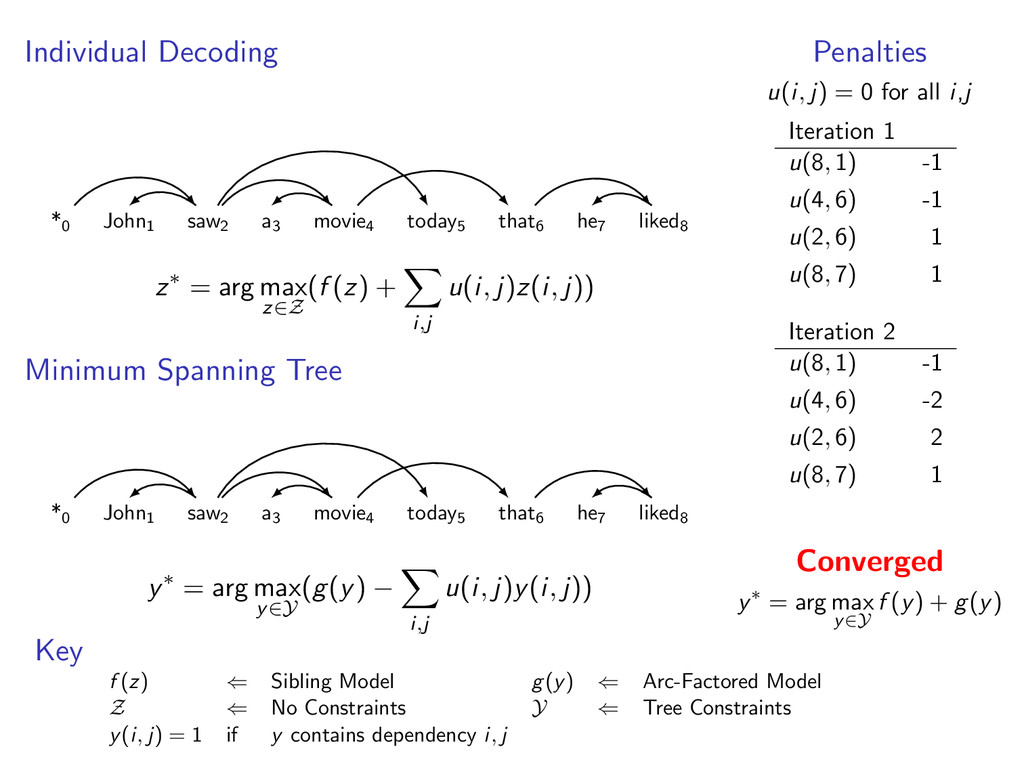
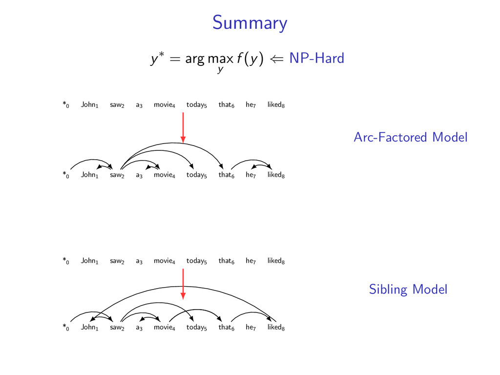
liked8 z∗ = arg max z∈Z (f (z) + i,j u(i, j)z(i, j)) Minimum Spanning Tree *0 John1 saw2 a3 movie4 today5 that6 he7 liked8 y∗ = arg max y∈Y (g(y) − i,j u(i, j)y(i, j)) Penalties u(i, j) = 0 for all i,j Key f (z) ⇐ Sibling Model g(y) ⇐ Arc-Factored Model Z ⇐ No Constraints Y ⇐ Tree Constraints y(i, j) = 1 if y contains dependency i, j
liked8 z∗ = arg max z∈Z (f (z) + i,j u(i, j)z(i, j)) Minimum Spanning Tree *0 John1 saw2 a3 movie4 today5 that6 he7 liked8 y∗ = arg max y∈Y (g(y) − i,j u(i, j)y(i, j)) Penalties u(i, j) = 0 for all i,j Key f (z) ⇐ Sibling Model g(y) ⇐ Arc-Factored Model Z ⇐ No Constraints Y ⇐ Tree Constraints y(i, j) = 1 if y contains dependency i, j
liked8 z∗ = arg max z∈Z (f (z) + i,j u(i, j)z(i, j)) Minimum Spanning Tree *0 John1 saw2 a3 movie4 today5 that6 he7 liked8 y∗ = arg max y∈Y (g(y) − i,j u(i, j)y(i, j)) Penalties u(i, j) = 0 for all i,j Key f (z) ⇐ Sibling Model g(y) ⇐ Arc-Factored Model Z ⇐ No Constraints Y ⇐ Tree Constraints y(i, j) = 1 if y contains dependency i, j
liked8 z∗ = arg max z∈Z (f (z) + i,j u(i, j)z(i, j)) Minimum Spanning Tree *0 John1 saw2 a3 movie4 today5 that6 he7 liked8 y∗ = arg max y∈Y (g(y) − i,j u(i, j)y(i, j)) Penalties u(i, j) = 0 for all i,j Key f (z) ⇐ Sibling Model g(y) ⇐ Arc-Factored Model Z ⇐ No Constraints Y ⇐ Tree Constraints y(i, j) = 1 if y contains dependency i, j
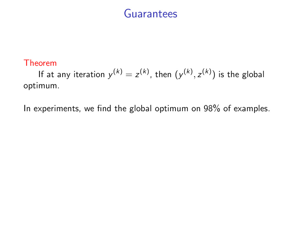
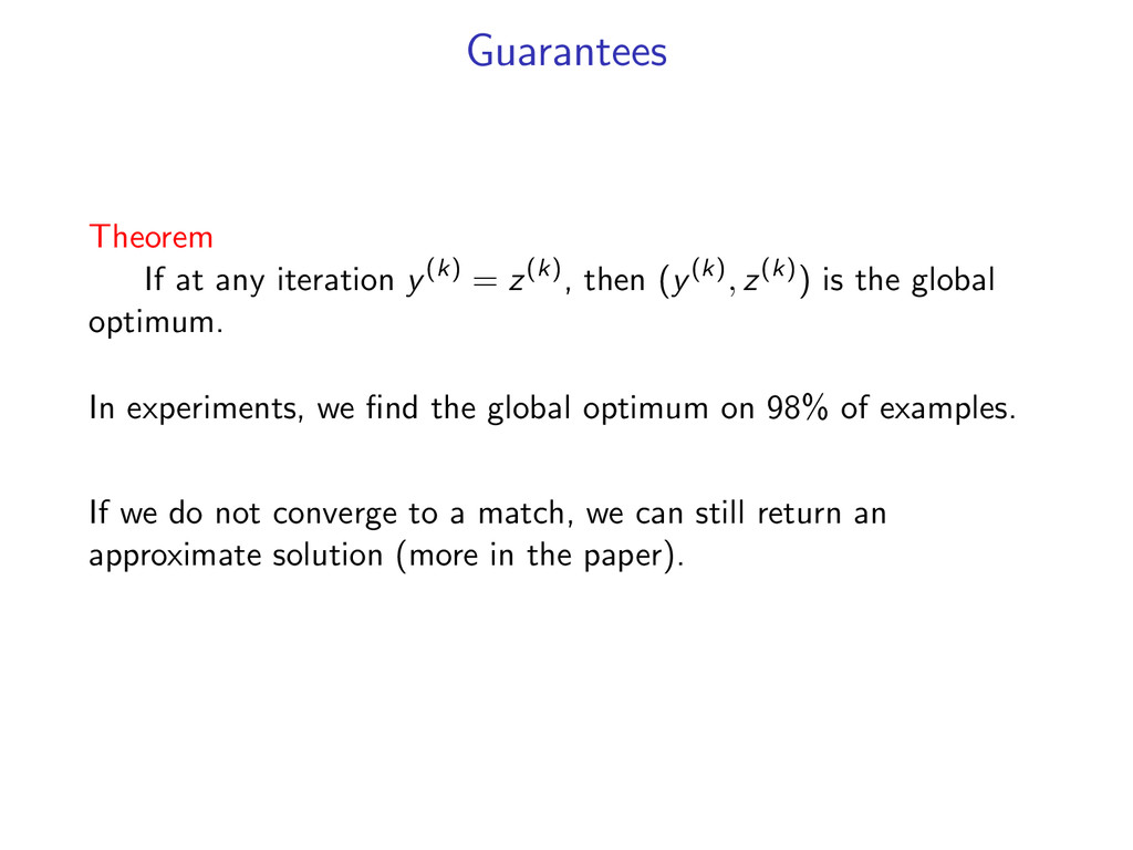
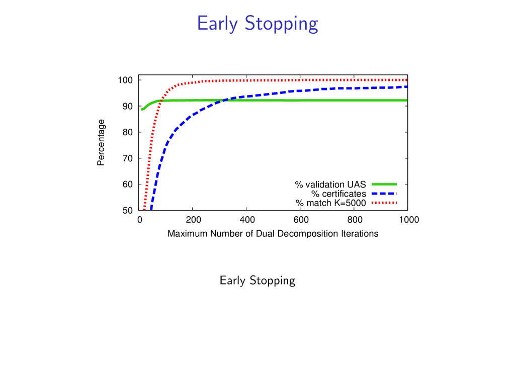
(y(k), z(k)) is the global optimum. In experiments, we find the global optimum on 98% of examples. If we do not converge to a match, we can still return an approximate solution (more in the paper).
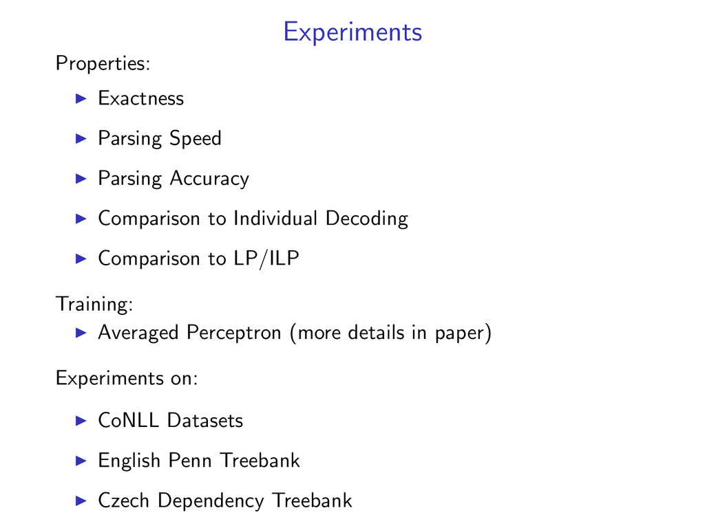
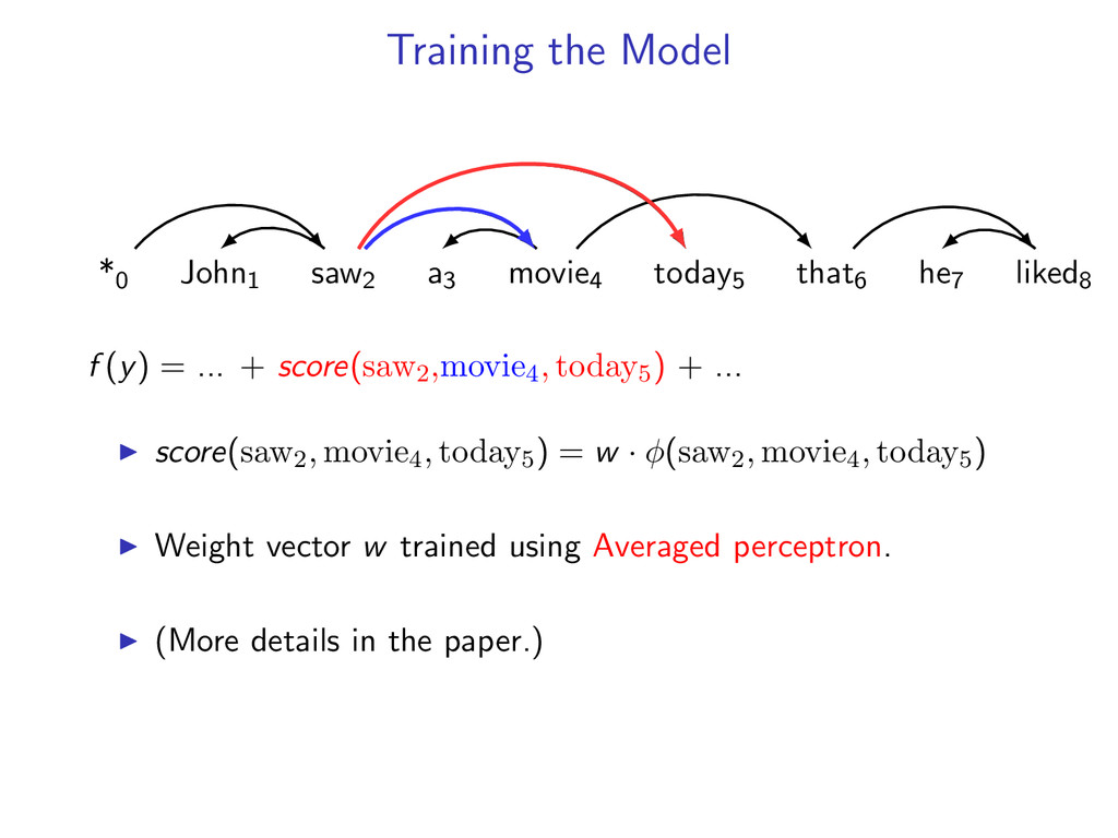
Decoding Comparison to LP/ILP Training: Averaged Perceptron (more details in paper) Experiments on: CoNLL Datasets English Penn Treebank Czech Dependency Treebank
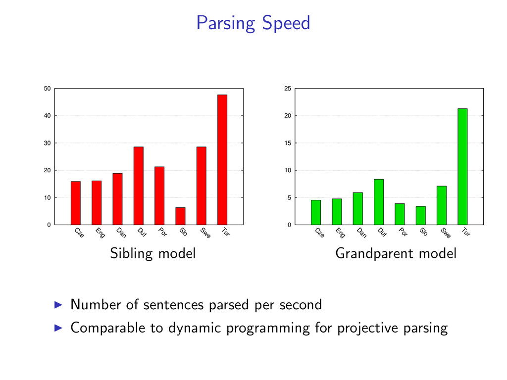
Eng D an D ut Por Slo Sw e Tur Sibling model 0 5 10 15 20 25 C ze Eng D an D ut Por Slo Sw e Tur Grandparent model Number of sentences parsed per second Comparable to dynamic programming for projective parsing
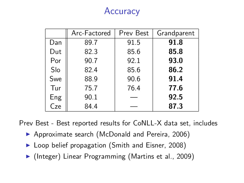
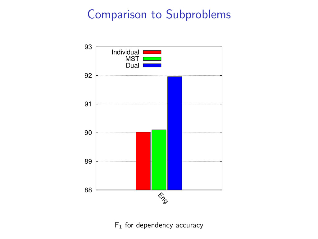
82.3 85.6 85.8 Por 90.7 92.1 93.0 Slo 82.4 85.6 86.2 Swe 88.9 90.6 91.4 Tur 75.7 76.4 77.6 Eng 90.1 — 92.5 Cze 84.4 — 87.3 Prev Best - Best reported results for CoNLL-X data set, includes Approximate search (McDonald and Pereira, 2006) Loop belief propagation (Smith and Eisner, 2008) (Integer) Linear Programming (Martins et al., 2009)
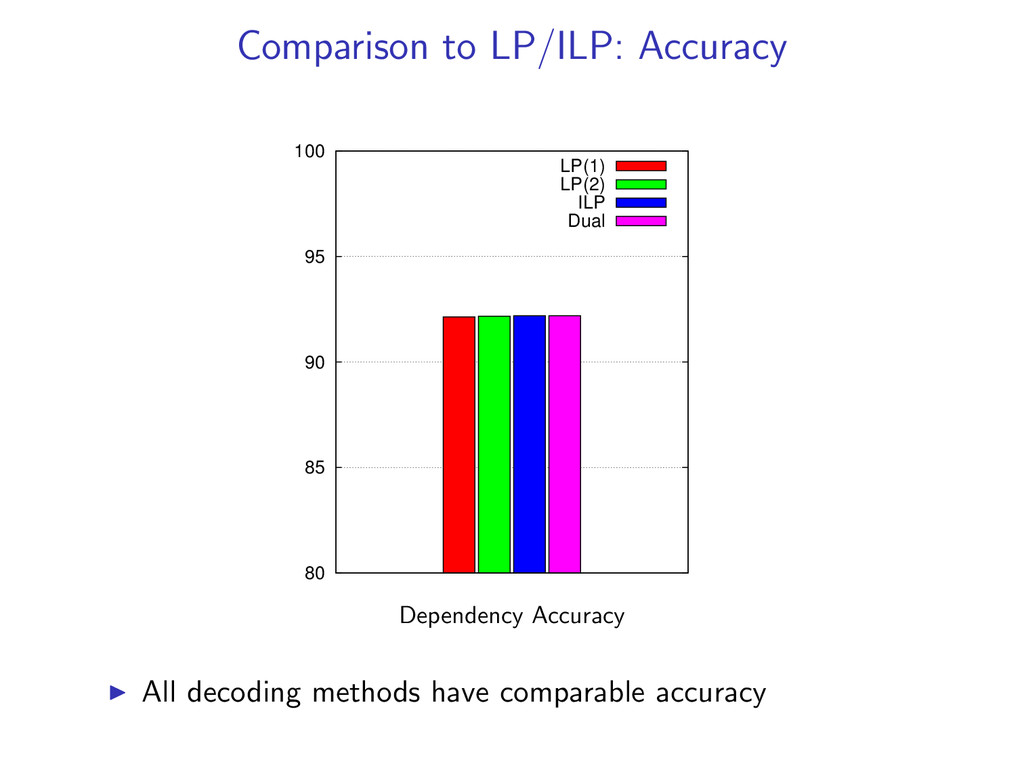
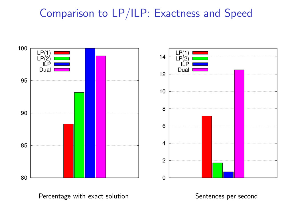
non-projective dependency parsing as a linear programming relaxation as well as an exact ILP. LP (1) LP (2) ILP Use an LP/ILP Solver for decoding We compare: Accuracy Exactness Speed Both LP and dual decomposition methods use the same model, features, and weights w.
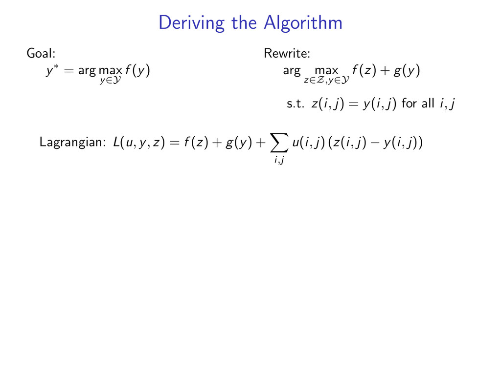
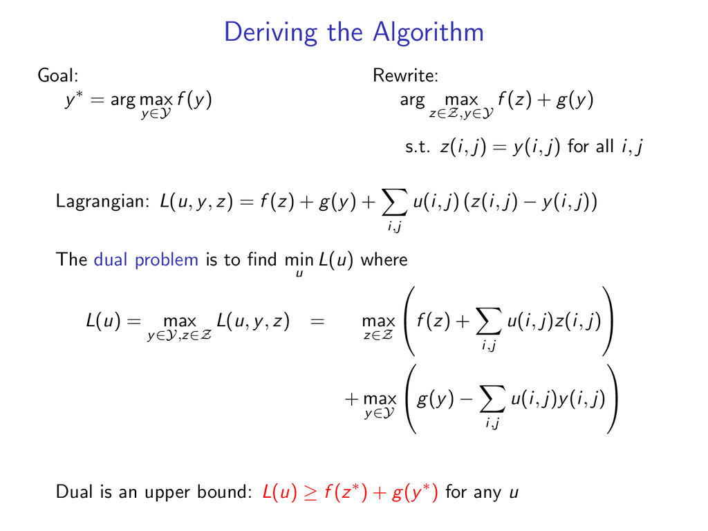
(y) Rewrite: arg max z∈Z,y∈Y f (z) + g(y) s.t. z(i, j) = y(i, j) for all i, j Lagrangian: L(u, y, z) = f (z) + g(y) + i,j u(i, j) (z(i, j) − y(i, j)) The dual problem is to find min u L(u) where L(u) = max y∈Y,z∈Z L(u, y, z) = max z∈Z f (z) + i,j u(i, j)z(i, j) + max y∈Y g(y) − i,j u(i, j)y(i, j) Dual is an upper bound: L(u) ≥ f (z∗) + g(y∗) for any u
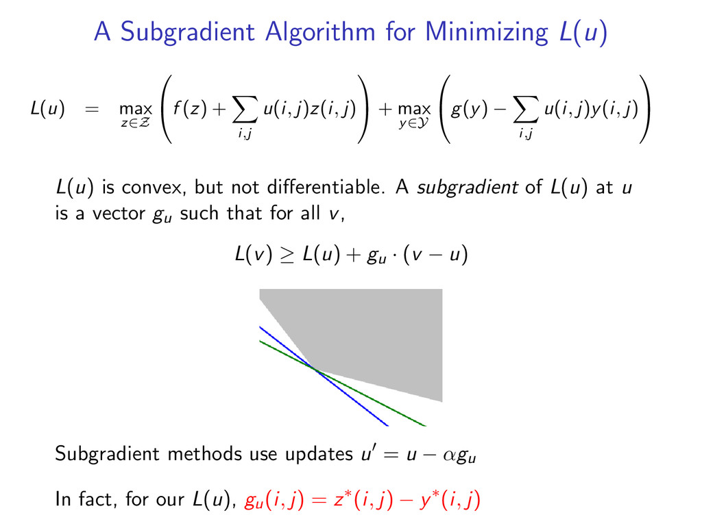
f (z) + i,j u(i, j)z(i, j) + max y∈Y g(y) − i,j u(i, j)y(i, j) L(u) is convex, but not differentiable. A subgradient of L(u) at u is a vector gu such that for all v, L(v) ≥ L(u) + gu · (v − u) Subgradient methods use updates u = u − αgu In fact, for our L(u), gu(i, j) = z∗(i, j) − y∗(i, j)
integer linear programming solvers (Martins et al. 2009; Riedel and Clarke 2006; Roth and Yih 2005) Dual decomposition/Lagrangian relaxation in combinatorial optimization (Dantzig and Wolfe, 1960; Held and Karp, 1970; Fisher 1981) Dual decomposition for inference in MRFs (Komodakis et al., 2007; Wainwright et al., 2005) Methods that incorporate combinatorial solvers within loopy belief propagation (Duchi et al. 2007; Smith and Eisner 2008)
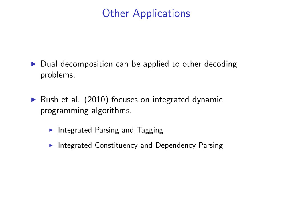
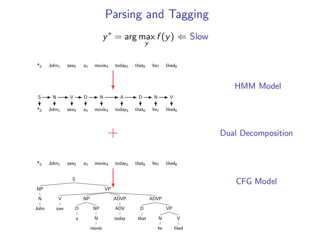
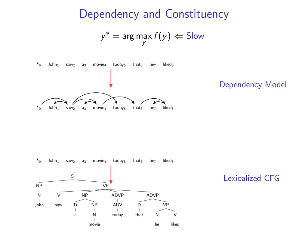
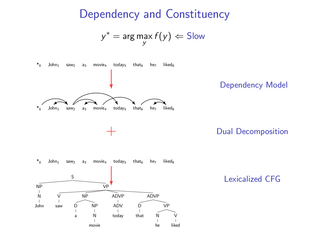
problems. Rush et al. (2010) focuses on integrated dynamic programming algorithms. Integrated Parsing and Tagging Integrated Constituency and Dependency Parsing
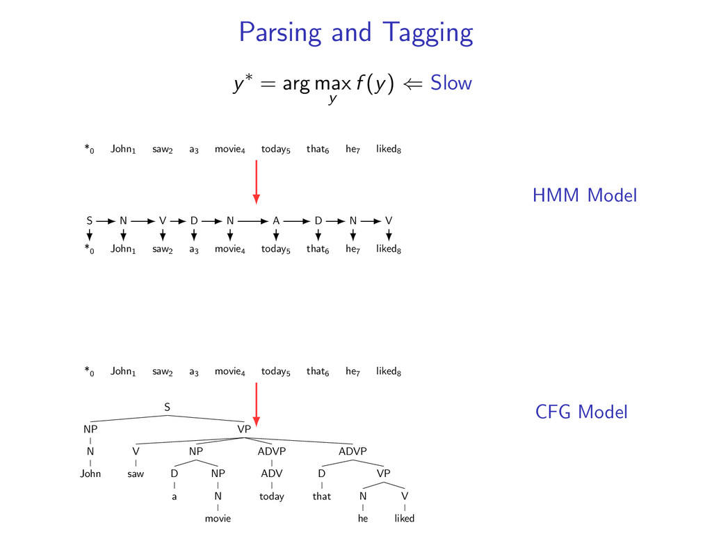
⇐ Slow *0 John1 saw2 a3 movie4 today5 that6 he7 liked8 *0 John1 saw2 a3 movie4 today5 that6 he7 liked8 S N V D N A D N V *0 John1 saw2 a3 movie4 today5 that6 he7 liked8 S NP N John VP V saw NP D a NP N movie ADVP ADV today ADVP D that VP N he V liked HMM Model CFG Model
⇐ Slow *0 John1 saw2 a3 movie4 today5 that6 he7 liked8 *0 John1 saw2 a3 movie4 today5 that6 he7 liked8 S N V D N A D N V + *0 John1 saw2 a3 movie4 today5 that6 he7 liked8 S NP N John VP V saw NP D a NP N movie ADVP ADV today ADVP D that VP N he V liked HMM Model Dual Decomposition CFG Model
⇐ Slow *0 John1 saw2 a3 movie4 today5 that6 he7 liked8 *0 John1 saw2 a3 movie4 today5 that6 he7 liked8 *0 John1 saw2 a3 movie4 today5 that6 he7 liked8 S NP N John VP V saw NP D a NP N movie ADVP ADV today ADVP D that VP N he V liked Dependency Model Lexicalized CFG
⇐ Slow *0 John1 saw2 a3 movie4 today5 that6 he7 liked8 *0 John1 saw2 a3 movie4 today5 that6 he7 liked8 + *0 John1 saw2 a3 movie4 today5 that6 he7 liked8 S NP N John VP V saw NP D a NP N movie ADVP ADV today ADVP D that VP N he V liked Dependency Model Dual Decomposition Lexicalized CFG
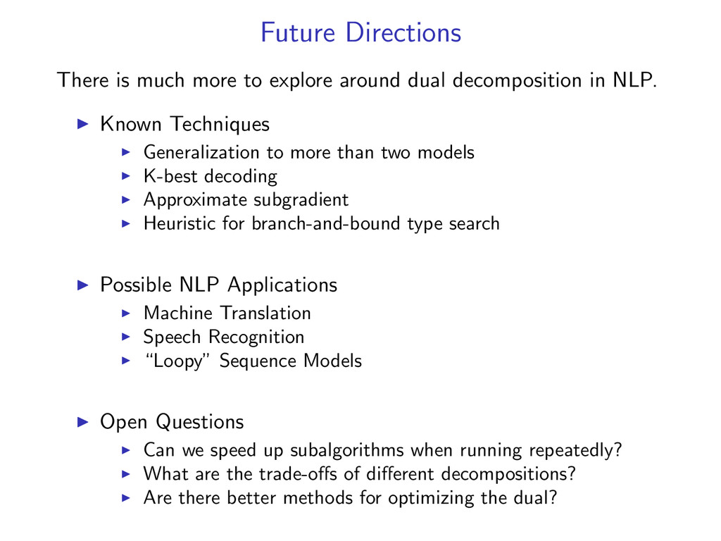
decomposition in NLP. Known Techniques Generalization to more than two models K-best decoding Approximate subgradient Heuristic for branch-and-bound type search Possible NLP Applications Machine Translation Speech Recognition “Loopy” Sequence Models Open Questions Can we speed up subalgorithms when running repeatedly? What are the trade-offs of different decompositions? Are there better methods for optimizing the dual?