Kaggle_Days_Tokyo_-_Feature_Engineering_and_GBDT_Implementation.pdf

Transcript

1. Feature Engineering Techniques and GBDT Implementation Daisuke Kadowaki
2. Self introduction • https://www.kaggle.com/threecourse • Kaggle Competitions Master (Walmart Recruiting II Winner, Coupon Purchase Prediction 3rd) • author of “Data Analysis Techniques to Win Kaggle” (book written in Japanese) • organizer of Kaggle Meetup Tokyo • freelance engineer(?), used to be an actuary
3. Agenda • I. Feature Engineering Techniques About “Data Analysis Techniques to Win Kaggle” Some feature engineering techniques • II. Gradient Boosting Decision Tree Implementation Algorithm overview Implementation (in Kaggle Kernel) Algorithm variations and computational complexity
4. I. Feature Engineering Techniques
5. Agenda - I. Feature Engineering Techniques 1. Introduce “Data Analysis Techniques to Win Kaggle” 2. Categorize feature engineering techniques 3. Aggregate and calculate statistics 4. Other techniques and ideas
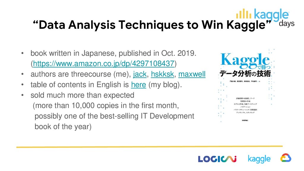
6. “Data Analysis Techniques to Win Kaggle” • book written in Japanese, published in Oct. 2019. (https://www.amazon.co.jp/dp/4297108437) • authors are threecourse (me), jack, hskksk, maxwell • table of contents in English is here (my blog). • sold much more than expected (more than 10,000 copies in the first month, possibly one of the best-selling IT Development book of the year)
7. Why sold so well? - simply great readable and comprehensive - covering intermediate level contents books for beginners are too many, but for intermediates are few. - Kaggle is catchy many data scientists know and are interested in Kaggle, even though might not want to participate. - insights from Kaggle are useful not only for competition, also for business especially, evaluation metrics and validation methods are well received.
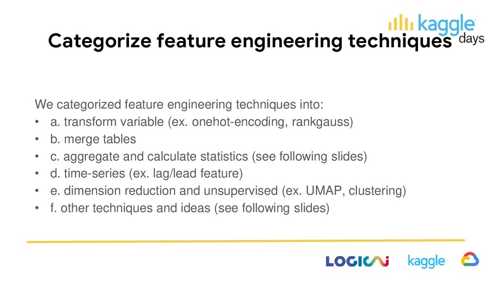
8. Categorize feature engineering techniques We categorized feature engineering techniques into: • a. transform variable (ex. onehot-encoding, rankgauss) • b. merge tables • c. aggregate and calculate statistics (see following slides) • d. time-series (ex. lag/lead feature) • e. dimension reduction and unsupervised (ex. UMAP, clustering) • f. other techniques and ideas (see following slides)
9. Aggregate and calculate statistics (excerpt from 3.9 aggregation and statistics) How to aggregate and create feature from transaction data? user master user log – to be aggregated
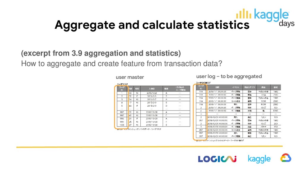
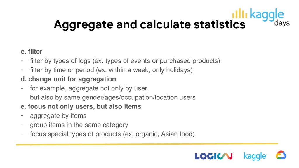
10. Aggregate and calculate statistics a. simple statistics - count, unique count, exist or not - sum, average, ratio - max, min, std, median, quantile, kurtosis, skewness b. statistics using temporal information (ex. for log data) - first, most recent - interval, frequency - interval and record just after key events - focusing on order, transition, cooccurrence, repetition
11. Aggregate and calculate statistics c. filter - filter by types of logs (ex. types of events or purchased products) - filter by time or period (ex. within a week, only holidays) d. change unit for aggregation - for example, aggregate not only by user, but also by same gender/ages/occupation/location users e. focus not only users, but also items - aggregate by items - group items in the same category - focus special types of products (ex. organic, Asian food)
12. Other techniques and ideas (excerpt some topics from 3.12 other techniques) 3.12.1 focus on mechanisms underlying • consider user's behavior • consider service provider’s behavior • check common practice in the industry (ex. disease diagnostic criteria) • combining variables to create an index (ex. Body Mass Index from height and weight) • consider mechanism of natural phenomena • try out the service of competition host by yourself
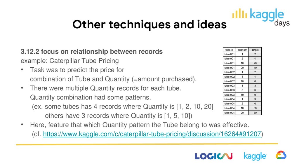
13. Other techniques and ideas 3.12.2 focus on relationship between records example: Caterpillar Tube Pricing • Task was to predict the price for combination of Tube and Quantity (=amount purchased). • There were multiple Quantity records for each tube. Quantity combination had some patterns. (ex. some tubes has 4 records where Quantity is [1, 2, 10, 20] others have 3 records where Quantity is [1, 5, 10]) • Here, feature that which Quantity pattern the Tube belong to was effective. (cf. https://www.kaggle.com/c/caterpillar-tube-pricing/discussion/16264#91207) tube-id quantity target tube-001 1 2 tube-001 2 4 tube-001 10 20 tube-001 20 40 tube-002 1 2 tube-002 5 4 tube-002 10 6 tube-003 1 3 tube-003 5 6 tube-003 10 9 tube-004 1 3 tube-004 2 6 tube-004 10 30 tube-004 20 60
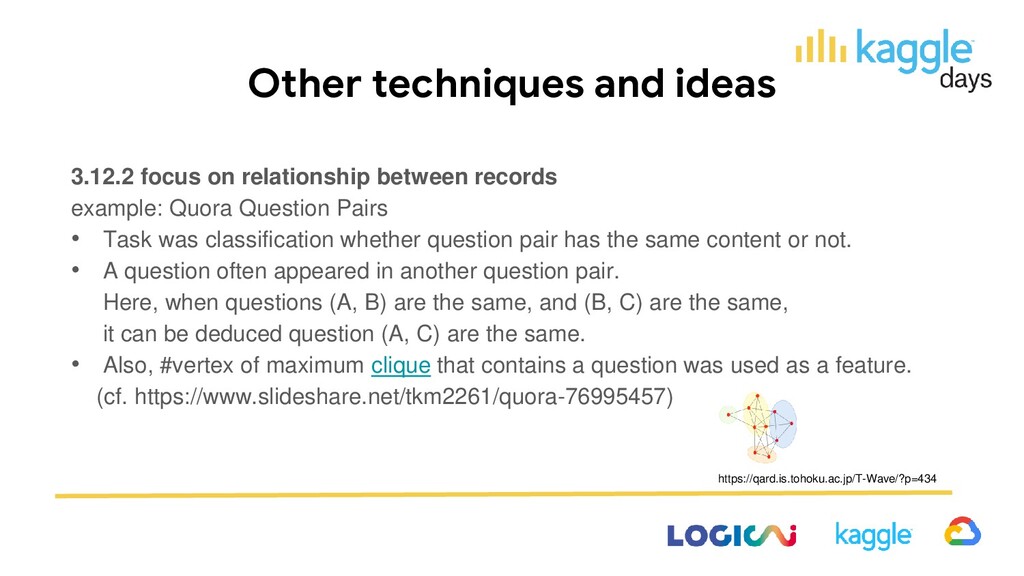
14. Other techniques and ideas 3.12.2 focus on relationship between records example: Quora Question Pairs • Task was classification whether question pair has the same content or not. • A question often appeared in another question pair. Here, when questions (A, B) are the same, and (B, C) are the same, it can be deduced question (A, C) are the same. • Also, #vertex of maximum clique that contains a question was used as a feature. (cf. https://www.slideshare.net/tkm2261/quora-76995457) https://qard.is.tohoku.ac.jp/T-Wave/?p=434
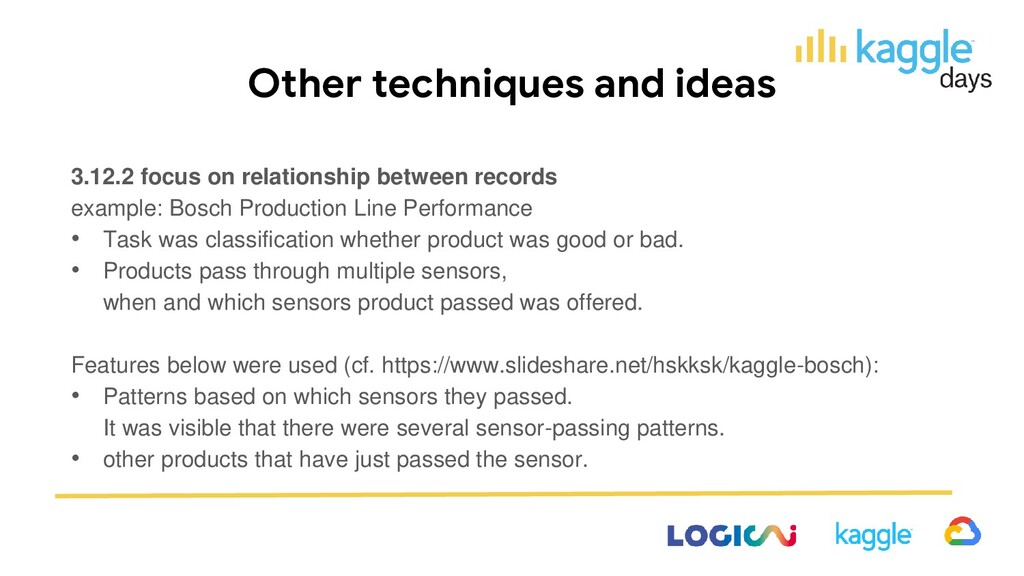
15. Other techniques and ideas 3.12.2 focus on relationship between records example: Bosch Production Line Performance • Task was classification whether product was good or bad. • Products pass through multiple sensors, when and which sensors product passed was offered. Features below were used (cf. https://www.slideshare.net/hskksk/kaggle-bosch): • Patterns based on which sensors they passed. It was visible that there were several sensor-passing patterns. • other products that have just passed the sensor.
16. Other techniques and ideas 3.12.3 focus on relative values • difference and ratio of price compared to average of same product/category/user/location (ex. Avito Demand Prediction Challenge, 9th solution) • loan amount compared to average of same occupation users. (ex. Home Credit Default Risk) • relative return compared to market average return (ex. Two Sigma Financial Modeling Challenge)
17. II. Gradient Boosting Implementation
18. Agenda - Gradient Boosting Implementation • Algorithm overview • Implementation (see Kaggle Kernel) • Algorithm variations and computational complexity
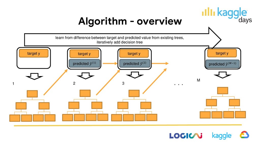
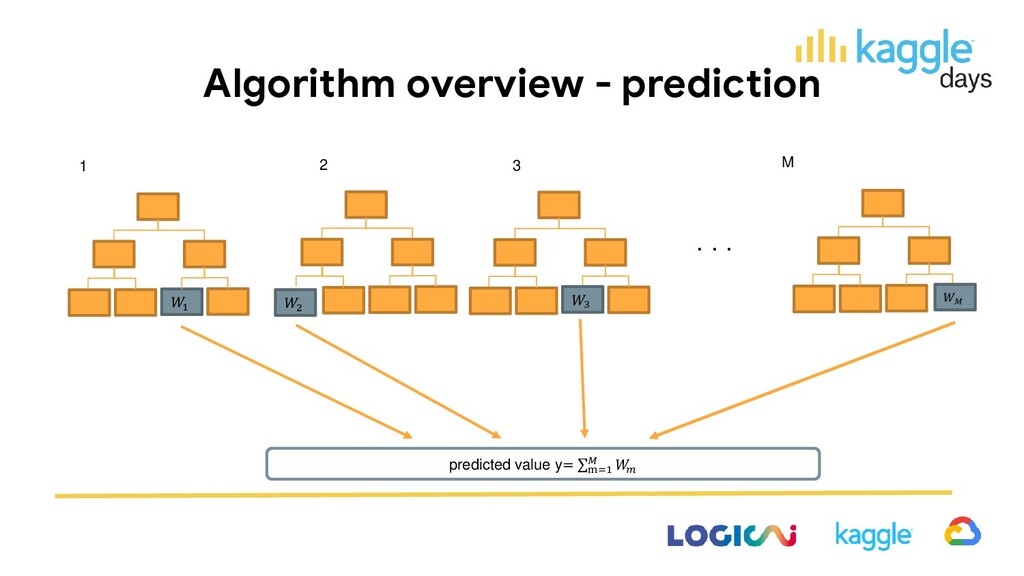
19. Algorithm - overview learn from difference between target and predicted value from existing trees, iteratively add decision tree ・・・ 1 2 M target y predicted ො (1) target y 3 predicted ො (2) target y predicted ො (−1) target y
20. Algorithm overview - prediction ・・・ 1 2 M 1 3 3 2 predicted value y= σm=1
21. Algorithm overview - prediction How to predict with weights of the trees? Regression: predicted value is ( is node weight of k-th tree and i-th data) Classification: predicted probability is
22. Algorithm overview – gradient and hessian How to calculate gradients and hessian? (note: regularization omitted) Regression – objective function RMSE: objective: gradient: hessian: Classification – objective function logloss: objective: gradient : hessian : here,
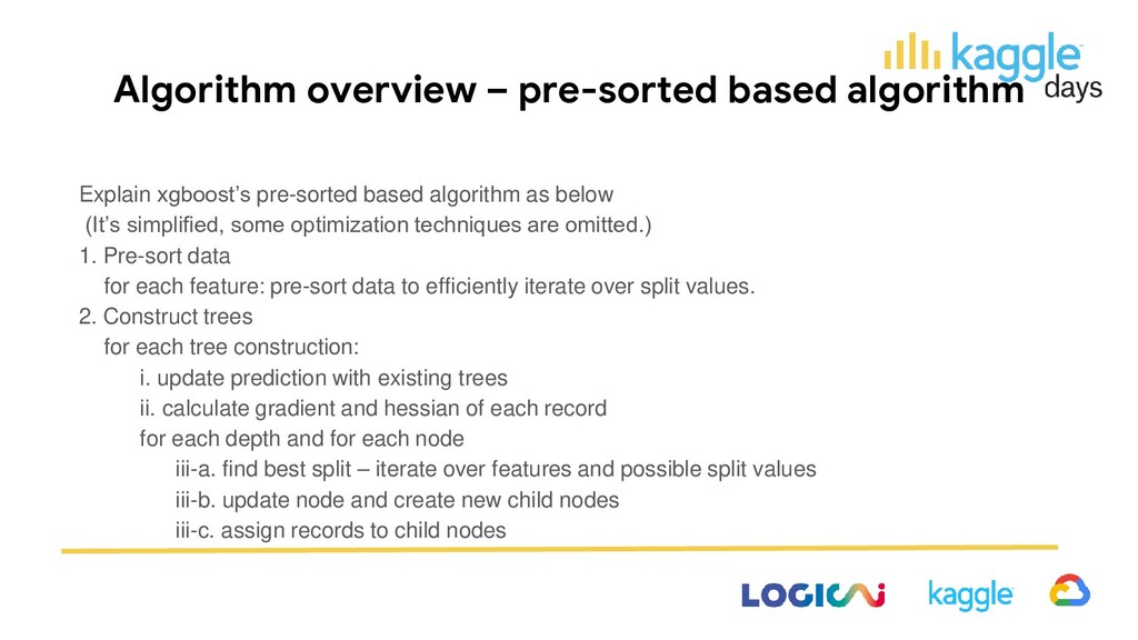
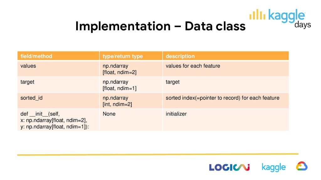
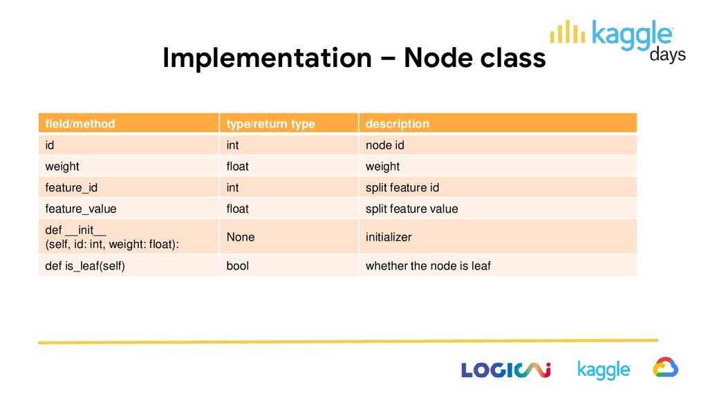
23. Algorithm overview – pre-sorted based algorithm Explain xgboost’s pre-sorted based algorithm as below (It’s simplified, some optimization techniques are omitted.) 1. Pre-sort data for each feature: pre-sort data to efficiently iterate over split values. 2. Construct trees for each tree construction: i. update prediction with existing trees ii. calculate gradient and hessian of each record for each depth and for each node iii-a. find best split – iterate over features and possible split values iii-b. update node and create new child nodes iii-c. assign records to child nodes
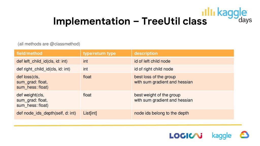
24. Algorithm overview – find best split Finding best split is the key of the algorithm. How to decide the best split? • Best weight and loss of the group can be approximately calculated with sum of gradient and hessian of the group. (note: constant term and regularization omitted) • Thus, when the split is decided and divide groups into two nodes, the best weight and loss of the new two nodes can be calculated. • Find iteratively over features and possible split values, efficiently with pre-sorted data. • The best split which yields the minimum sum loss of the new two groups is chosen. (cf. XGBoost: A Scalable Tree Boosting System 2.2 Gradient Tree Boosting) best weight and loss: objective function:
25. Implementation Here, explain simple implementation of xgboost’s pre-sorted based algorithm . see Kaggle Kernel: https://www.kaggle.com/threecourse/gbdt-implementation-kaggle-days-tokyo https://www.kaggle.com/threecourse/gbdt-implementation-cython-kaggle-days-tokyo
26. Implementation – Data class field/method type/return type description values np.ndarray [float, ndim=2] values for each feature target np.ndarray [float, ndim=1] target sorted_id np.ndarray [int, ndim=2] sorted index(=pointer to record) for each feature def __init__(self, x: np.ndarray[float, ndim=2], y: np.ndarray[float, ndim=1]): None initializer
27. Implementation – Node class field/method type/return type description id int node id weight float weight feature_id int split feature id feature_value float split feature value def __init__ (self, id: int, weight: float): None initializer def is_leaf(self) bool whether the node is leaf
28. Implementation – TreeUtil class (all methods are @classmethod) field/method type/return type description def left_child_id(cls, id: int) int id of left child node def right_child_id(cls, id: int) int id of right child node def loss(cls, sum_grad: float, sum_hess: float) float best loss of the group with sum gradient and hessian def weight(cls, sum_grad: float, sum_hess: float) float best weight of the group with sum gradient and hessian def node_ids_depth(self, d: int) List[int] node ids belong to the depth
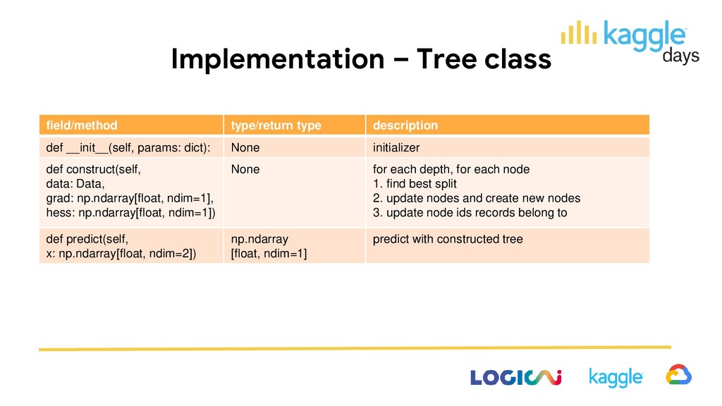
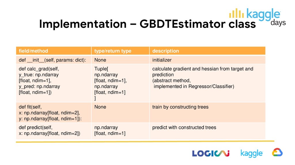
29. Implementation – Tree class field/method type/return type description def __init__(self, params: dict): None initializer def construct(self, data: Data, grad: np.ndarray[float, ndim=1], hess: np.ndarray[float, ndim=1]) None for each depth, for each node 1. find best split 2. update nodes and create new nodes 3. update node ids records belong to def predict(self, x: np.ndarray[float, ndim=2]) np.ndarray [float, ndim=1] predict with constructed tree
30. Implementation – GBDTEstimator class field/method type/return type description def __init__(self, params: dict): None initializer def calc_grad(self, y_true: np.ndarray [float, ndim=1], y_pred: np.ndarray [float, ndim=1]) Tuple[ np.ndarray [float, ndim=1], np.ndarray [float, ndim=1] ] calculate gradient and hessian from target and prediction (abstract method, implemented in Regressor/Classifier) def fit(self, x: np.ndarray[float, ndim=2], y: np.ndarray[float, ndim=1]): None train by constructing trees def predict(self, x: np.ndarray[float, ndim=2]) np.ndarray [float, ndim=1] predict with constructed trees
31. Implementation – GBDTClassifier class (inherits GBDTEstimator class) field/method type/return type description def calc_grad(self, y_true: np.ndarray [float, ndim=1], y_pred: np.ndarray [float, ndim=1]) Tuple[ np.ndarray [float, ndim=1], np.ndarray [float, ndim=1] ] calculate gradient and hessian from target and prediction def predict_proba (self, x: np.ndarray[float, ndim=2]) np.ndarray [float, ndim=1] predict probability with constructed trees
32. Implementation – use Cython Python implementation is not fast, Cython can be used for fast calculation. Tips are: • focus on inner loops • make function called frequently into c-function • designate variable used frequently with c-type • make foreach loop into simple range loop
33. Implementation - results Experimented on data of Otto Group Product Classification Challenge (converted into binary classification, class1-5 as 0 and class 6-9 as 1) train/valid: 10,000 records each, cpu: i9-9900K parameter time logloss xgboost round:125, max_depth_5, eta:0.1, subsample: 0.8, colsample_bytree:0.8, n_thread:1 2.8s 0.1706 simpleBoost round:125, max_depth_5, eta:0.1 1318.4s 0.1706 simpleBoost （w/ Cython) round:125, max_depth_5, eta:0.1 10.6s 0.1707
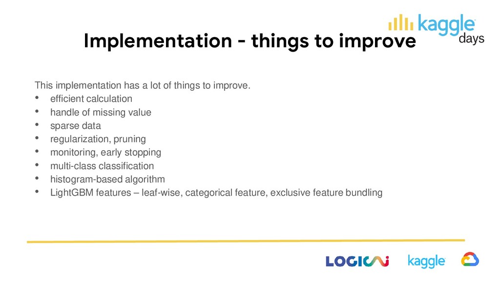
34. Implementation - things to improve This implementation has a lot of things to improve. • efficient calculation • handle of missing value • sparse data • regularization, pruning • monitoring, early stopping • multi-class classification • histogram-based algorithm • LightGBM features – leaf-wise, categorical feature, exclusive feature bundling
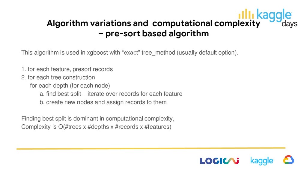
35. Algorithm variations and computational complexity – pre-sort based algorithm This algorithm is used in xgboost with “exact” tree_method (usually default option). 1. for each feature, presort records 2. for each tree construction for each depth (for each node) a. find best split – iterate over records for each feature b. create new nodes and assign records to them Finding best split is dominant in computational complexity, Complexity is O(#trees x #depths x #records x #features)
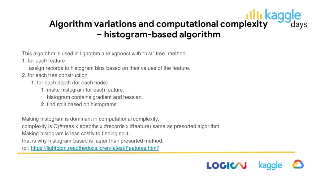
36. Algorithm variations and computational complexity – histogram-based algorithm This algorithm is used in lightgbm and xgboost with “hist” tree_method. 1. for each feature assign records to histogram bins based on their values of the feature. 2. for each tree construction 1. for each depth (for each node) 1. make histogram for each feature. histogram contains gradient and hessian. 2. find split based on histograms Making histogram is dominant in computational complexity, complexity is O(#trees x #depths x #records x #feature) same as presorted algorithm. Making histogram is less costly to finding split, that is why histogram-based is faster than presorted method. (cf. https://lightgbm.readthedocs.io/en/latest/Features.html)
37. This technique is used in lightgbm. Bundle “exclusive features” to reduce computational complexity. “exclusive features” are features which don’t have values other than 0 at the same time. with EFB, • complexity of making histogram O(#feature x #records) -> O(#bundles x #records) • when finding splits, bundled features are unbundled and original features are used. Algorithm variations and computational complexity – EFB(Exclusive Feature Bundling)
38. XGBoost: A Scalable Tree Boosting System https://www.kdd.org/kdd2016/papers/files/rfp0697-chenAemb.pdf LightGBM: A Highly Efficient Gradient Boosting Decision Tree https://papers.nips.cc/paper/6907-lightgbm-a-highly-efficient-gradient-boosting-decision-tree.pdf XGBoost documenatation https://xgboost.readthedocs.io/en/latest/index.html LightGBM documenatation https://lightgbm.readthedocs.io/en/latest A Gentle Introduction to XGBoost for Applied Machine Learning https://machinelearningmastery.com/gentle-introduction-xgboost-applied-machine-learning/ XGBoost Mathematics Explained https://towardsdatascience.com/xgboost-mathematics-explained-58262530904a A Kaggle Master Explains Gradient Boosting http://blog.kaggle.com/2017/01/23/a-kaggle-master-explains-gradient-boosting/ (in Japanese) NIPS2017読み会 LightGBM: A Highly Efficient Gradient Boosting Decision Tree https://www.slideshare.net/tkm2261/nips2017-lightgbm-a-highly-efficient-gradient-boosting-decision-tree XGBoostのお気持ちを一部理解する https://qiita.com/kenmatsu4/items/226f926d87de86c28089 References