Gaussian Splash - The world of 3D Gaussian Splatting

Transcript

1. Gaussian Splash The World of 3D Gaussian Splatting ushiostarfish
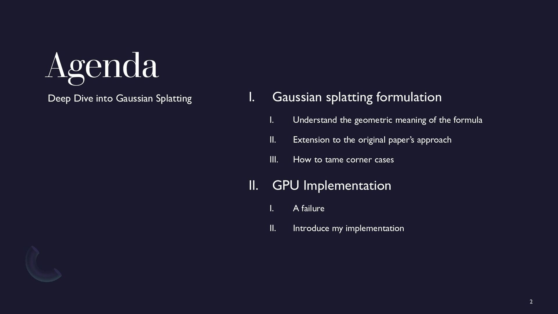
2. Agenda I. Gaussian splatting formulation I. Understand the geometric meaning of the formula II. Extension to the original paper’s approach III. How to tame corner cases II. GPU Implementation I. A failure II. Introduce my implementation Deep Dive into Gaussian Splatting
3. What’s gaussian splatting? • A method to represent a radiance field • A function of a location and a direction • Often calculated by 2d image set • Differentiable rendering ? ? 𝑓( Ԧ 𝑥, 𝜔) 𝑓( Ԧ 𝑥, 𝜔)
4. Gaussian? Scene geometry consists of semi-transparent ellipsoids
5. Gaussian? Scene geometry consists of semi-transparent ellipsoids
6. Gaussian? Scene geometry consists of semi-transparent ellipsoids 3d anisotropic Gaussian kernel Gaussian Splatting
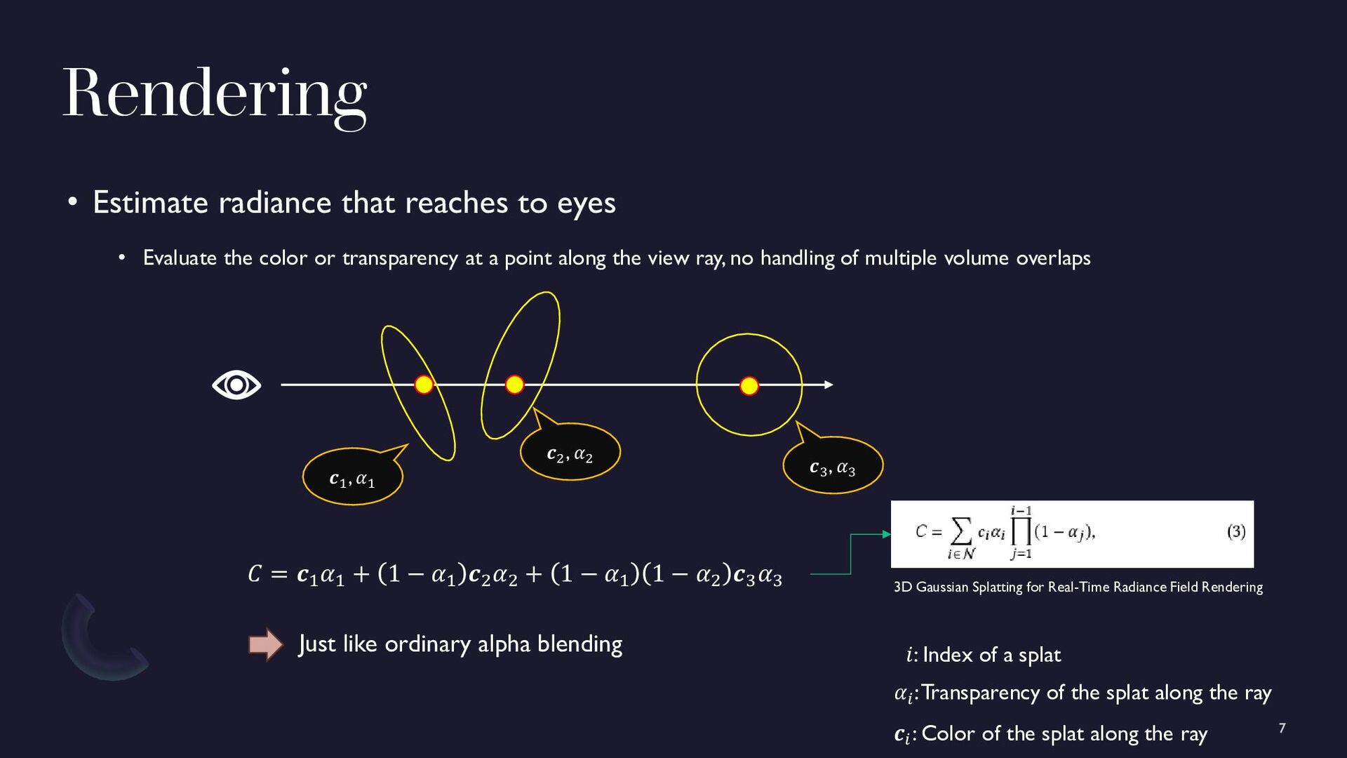
7. Rendering • Estimate radiance that reaches to eyes • Evaluate the color or transparency at a point along the view ray, no handling of multiple volume overlaps 𝒄1, 𝛼1 𝒄2, 𝛼2 𝒄3, 𝛼3 𝛼𝑖: Transparency of the splat along the ray 𝒄𝑖: Color of the splat along the ray 𝑖: Index of a splat 𝐶 = 𝒄1 𝛼1 + 1 − 𝛼1 𝒄2 𝛼2 + 1 − 𝛼1 1 − 𝛼2 𝒄3 𝛼3 Just like ordinary alpha blending 3D Gaussian Splatting for Real-Time Radiance Field Rendering
8. Multivariate Gaussian kernel 𝐺 𝒙 = 1 2𝜋 𝑑det(Σ) exp(− 1 2 𝒙 − 𝝁 𝑇Σ−1 𝒙 − 𝝁 ) Multivariate Gaussian distribution 𝐺𝑔𝑠 𝒙 = exp(− 1 2 𝒙 − 𝝁 𝑇Σ−1 𝒙 − 𝝁 ) Don’t have to be normalized A key component : Covariance Matrix Σ ? ? ? ? ? ? ? ? ? ? ? ? ?
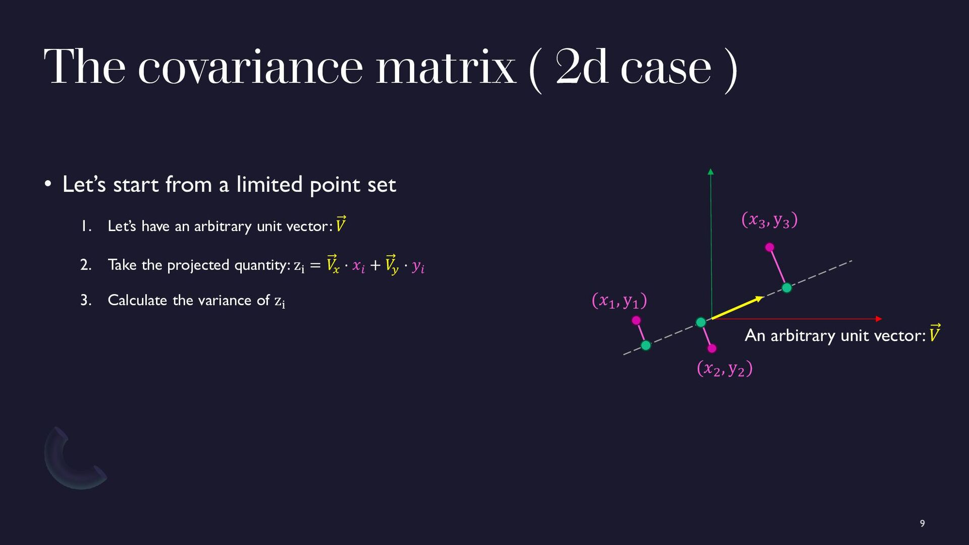
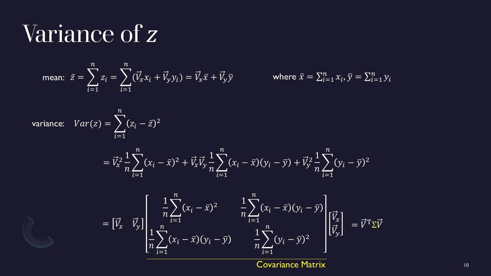
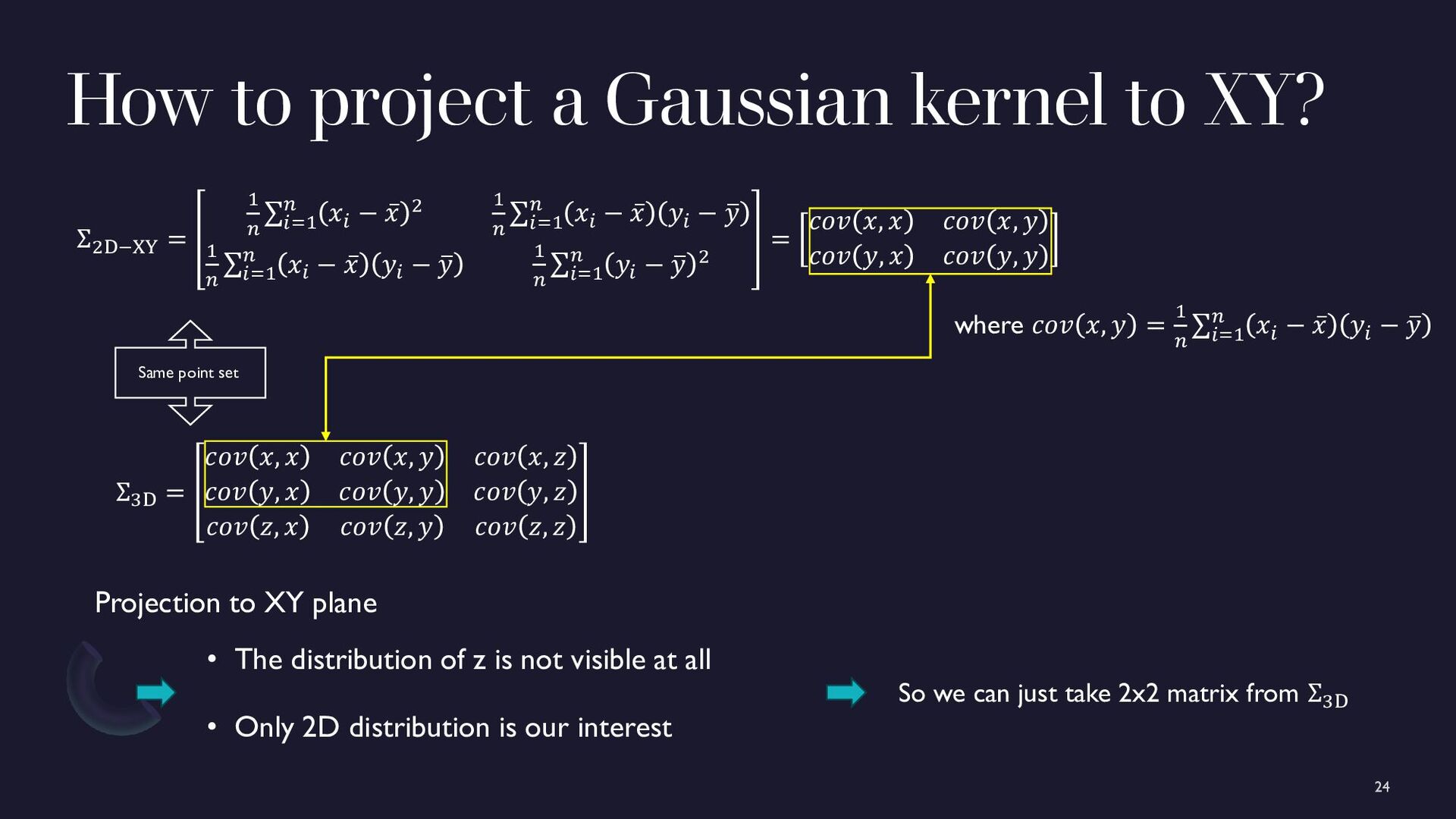
9. The covariance matrix ( 2d case ) • Let’s start from a limited point set 1. Let’s have an arbitrary unit vector: 𝑉 2. Take the projected quantity: zi = 𝑉 𝑥 ⋅ 𝑥𝑖 + 𝑉 𝑦 ⋅ 𝑦𝑖 3. Calculate the variance of zi An arbitrary unit vector: 𝑉 (𝑥1 , y1 ) (𝑥2 , y2 ) (𝑥3 , y3 )
10. Variance of 𝑧 ҧ 𝑧 = ෍ 𝑖=1 𝑛 𝑧𝑖 = ෍ 𝑖=1 𝑛 (𝑉 𝑥 𝑥𝑖 + 𝑉 𝑦 𝑦𝑖 ) = 𝑉 𝑥 ҧ 𝑥 + 𝑉 𝑦 ത 𝑦 mean: where ҧ 𝑥 = σ 𝑖=1 𝑛 𝑥𝑖, ത 𝑦 = σ 𝑖=1 𝑛 𝑦𝑖 variance: 𝑉𝑎𝑟(𝑧) = ෍ 𝑖=1 𝑛 𝑧𝑖 − ҧ 𝑧 2 = 𝑉 𝑥 2 1 𝑛 ෍ 𝑖=1 𝑛 𝑥𝑖 − ҧ 𝑥 2 + 𝑉 𝑥 𝑉 𝑦 1 𝑛 ෍ 𝑖=1 𝑛 𝑥𝑖 − ҧ 𝑥 𝑦𝑖 − ത 𝑦 + 𝑉 𝑦 2 1 𝑛 ෍ 𝑖=1 𝑛 𝑦𝑖 − ത 𝑦 2 = 𝑉 𝑥 𝑉 𝑦 1 𝑛 ෍ 𝑖=1 𝑛 𝑥𝑖 − ҧ 𝑥 2 1 𝑛 ෍ 𝑖=1 𝑛 𝑥𝑖 − ҧ 𝑥 𝑦𝑖 − ത 𝑦 1 𝑛 ෍ 𝑖=1 𝑛 𝑥𝑖 − ҧ 𝑥 𝑦𝑖 − ത 𝑦 1 𝑛 ෍ 𝑖=1 𝑛 𝑦𝑖 − ത 𝑦 2 𝑉 𝑥 𝑉 𝑦 Covariance Matrix = 𝑉TΣ𝑉
11. Identity covariance matrix ΣI = 1 0 0 1 𝐺𝑔𝑠 𝒙 = exp(− 1 2 𝒙 − 𝝁 𝑇ΣI −1 𝒙 − 𝝁 ) Just a one-dimensional Gaussian kernel! = exp(− 1 2 𝒙 − 𝝁 2) 𝒙 0 1 𝝁
12. Affine Transform of covariance matrix Looks like we can obtain a lot of various Gaussian kernels just with Affine Transforms? Idea: A lot of variations…
13. Apply a transform to a point set Σ = 1 𝑛 ෍ 𝑖=1 𝑛 𝑥𝑖 − ҧ 𝑥 2 1 𝑛 ෍ 𝑖=1 𝑛 𝑥𝑖 − ҧ 𝑥 𝑦𝑖 − ത 𝑦 1 𝑛 ෍ 𝑖=1 𝑛 𝑥𝑖 − ҧ 𝑥 𝑦𝑖 − ത 𝑦 1 𝑛 ෍ 𝑖=1 𝑛 𝑦𝑖 − ത 𝑦 2 = 1 𝑛 ෍ 𝑖=1 𝑛 𝑥𝑖 − ҧ 𝑥 2 𝑥𝑖 − ҧ 𝑥 𝑦𝑖 − ത 𝑦 𝑥𝑖 − ҧ 𝑥 𝑦𝑖 − ത 𝑦 𝑦𝑖 − ത 𝑦 2 = 1 𝑛 ෍ 𝑖=1 𝑛 ( 𝑥𝑖 − ҧ 𝑥 𝑦𝑖 − ത 𝑦 𝑥𝑖 − ҧ 𝑥 𝑦𝑖 − ത 𝑦 𝑇 ) 𝑥𝑖 ′ = 𝑀𝑥𝑖 𝑥1 , 𝑥2 , … 𝑥𝑖 𝑥′1 , 𝑥′2 , … 𝑥′𝑖 Σ′ = 1 𝑛 ෍ 𝑖=1 𝑛 𝑀 𝑥𝑖 − ҧ 𝑥 𝑦𝑖 − ത 𝑦 𝑀 𝑥𝑖 − ҧ 𝑥 𝑦𝑖 − ത 𝑦 𝑇 = 𝑀 1 𝑛 ෍ 𝑖=1 𝑛 𝑥𝑖 − ҧ 𝑥 2 𝑥𝑖 − ҧ 𝑥 𝑦𝑖 − ത 𝑦 𝑥𝑖 − ҧ 𝑥 𝑦𝑖 − ത 𝑦 𝑦𝑖 − ത 𝑦 2 𝑀𝑇 = 𝑀Σ𝑀𝑇 Just sandwich by M!
14. 𝒙 𝑀−1 𝒙′ Meaning of the distance 𝐺𝑔𝑠 𝒙 = exp(− 1 2 𝒙 − 𝝁 𝑇Σ−1 𝒙 − 𝝁 ) Multivariate Gaussian kernel = 𝒙 − 𝝁 𝑇 𝑀−1 𝑇 1 0 0 1 −1 𝑀−1 𝒙 − 𝝁 = 𝑀−1(𝒙 − 𝝁) 𝑇 1 0 0 1 −1 𝑀−1 𝒙 − 𝝁 Evaluate distance on identity kernel 𝒙 − 𝝁 𝑇Σ−1 𝒙 − 𝝁 = 𝒙 − 𝝁 𝑇 𝑀 1 0 0 1 𝑀𝑇 −1 𝒙 − 𝝁 Transformed Identity covariance matrix
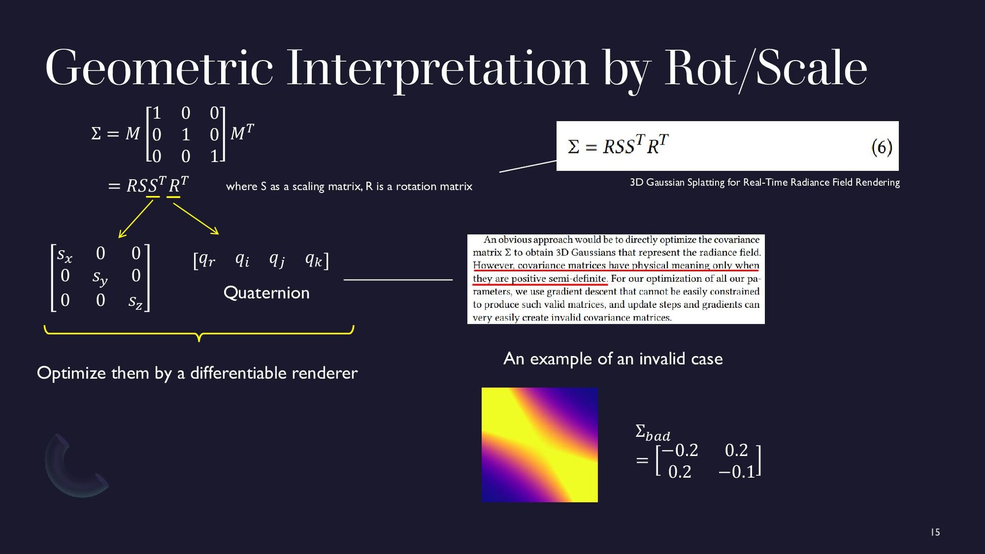
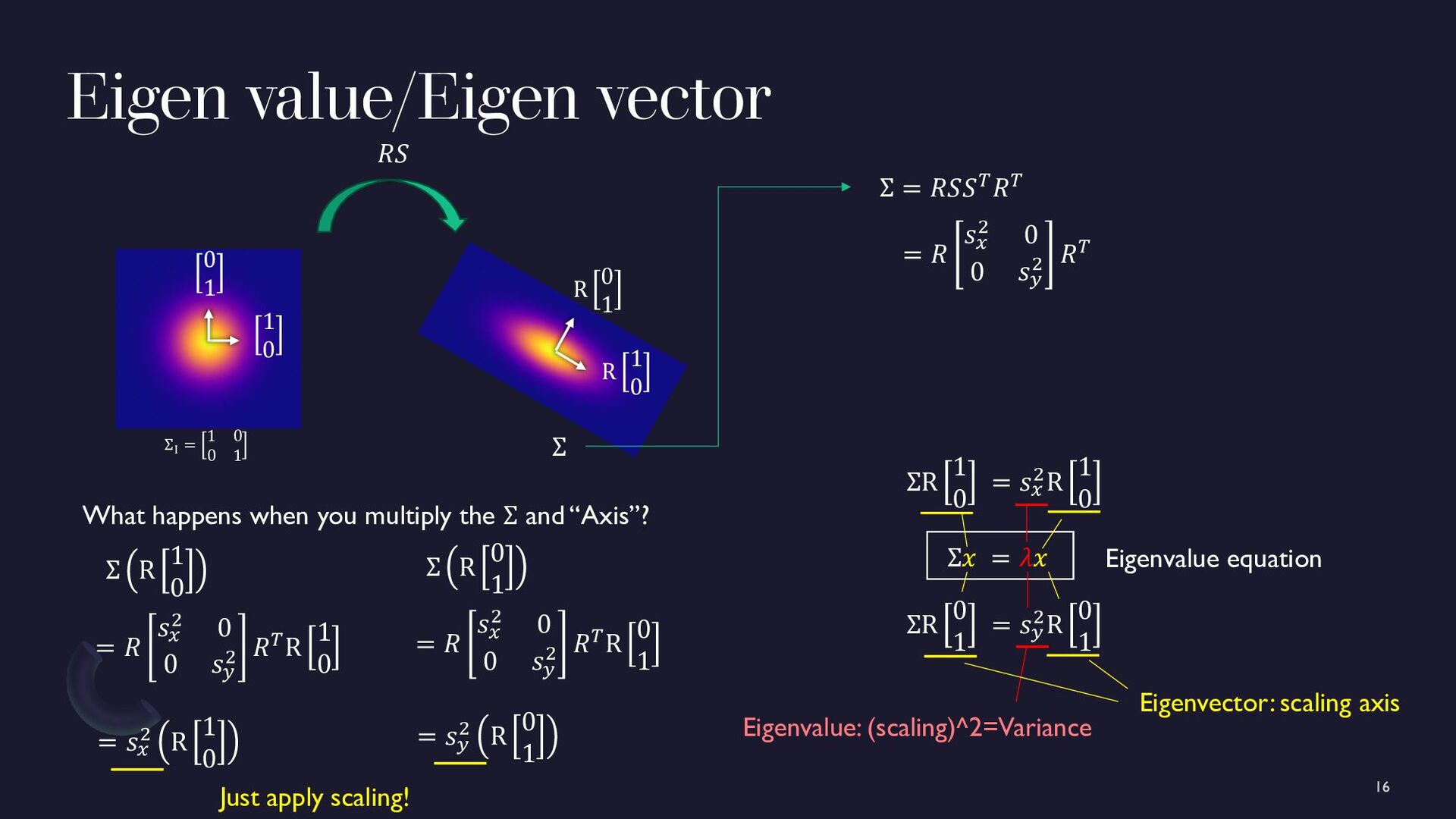
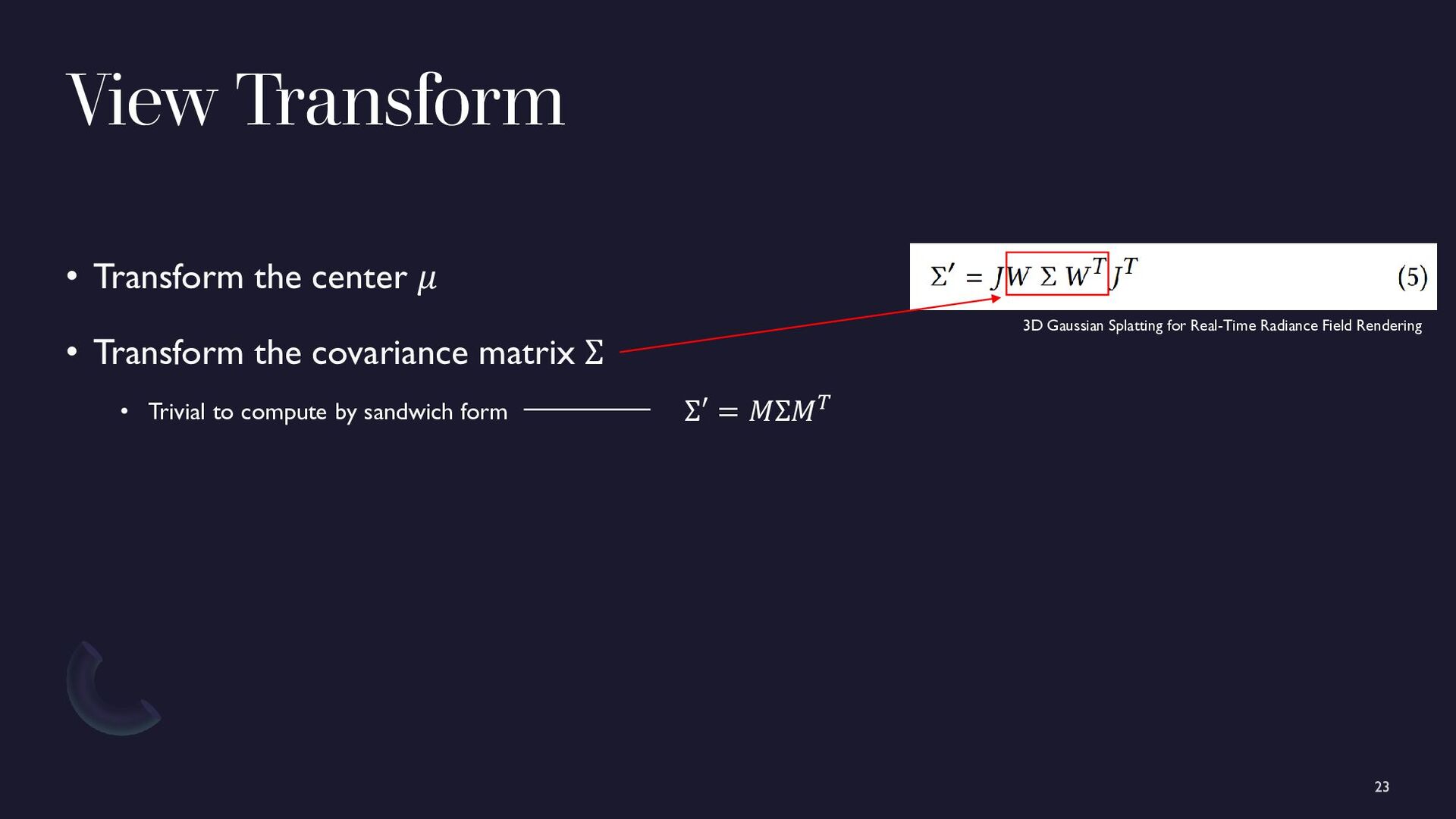
15. Geometric Interpretation by Rot/Scale Σ = 𝑀 1 0 0 0 1 0 0 0 1 𝑀𝑇 = 𝑅𝑆𝑆𝑇𝑅𝑇 where S as a scaling matrix, R is a rotation matrix 3D Gaussian Splatting for Real-Time Radiance Field Rendering 𝑠𝑥 0 0 0 𝑠𝑦 0 0 0 𝑠𝑧 Quaternion 𝑞𝑟 𝑞𝑖 𝑞𝑗 𝑞𝑘 Optimize them by a differentiable renderer Σ𝑏𝑎𝑑 = −0.2 0.2 0.2 −0.1 An example of an invalid case
16. Eigen value/Eigen vector = 𝑅 𝑠𝑥 2 0 0 𝑠𝑦 2 𝑅𝑇R 1 0 = 𝑠𝑥 2 R 1 0 = 𝑅 𝑠𝑥 2 0 0 𝑠𝑦 2 𝑅𝑇R 0 1 = 𝑠𝑦 2 R 0 1 Eigenvector: scaling axis ΣR 1 0 = 𝑠𝑥 2R 1 0 Σ𝑥 = 𝜆𝑥 ΣR 0 1 = 𝑠𝑦 2R 0 1 Eigenvalue equation Eigenvalue: (scaling)^2=Variance 𝑅𝑆 1 0 R 1 0 0 1 R 0 1 ΣI = 1 0 0 1 Σ Σ = 𝑅𝑆𝑆𝑇𝑅𝑇 = 𝑅 𝑠𝑥 2 0 0 𝑠𝑦 2 𝑅𝑇 What happens when you multiply the Σ and “Axis”? Σ R 1 0 Σ R 0 1 Just apply scaling!
17. Bounding box • You often need a bounding box of a splat • For rasterization ( 2d ) • The original paper’s implementation uses eigenvalue to find a conservative bound 𝒙 − 𝝁 𝑇Σ−1 𝒙 − 𝝁 = 𝟐𝟐 𝒙 − 𝝁 = 𝟐 𝒎𝒂𝒙(𝝀𝟏 , 𝝀𝟐 ) radius This is too conservative  https://github.com/graphdeco-inria/diff-gaussian- rasterization/blob/59f5f77e3ddbac3ed9db93ec2cfe99ed6c5d121d/cuda_rasterizer/forward.cu#L229-L232 Chapter 15 固有値の計算の小技 | 線形代数のエッセンス https://www.youtube.com/watch?v=VyVi7iPb1Uw&t=3s A quick trick for computing eigenvalues | Chapter 15, Essence of linear algebra https://www.youtube.com/watch?v=e50Bj7jn9IQ
18. Extension to the original GS
19. Tighter bounding box ƴ 𝑠11 𝑣𝑥 2 + 2 ƴ 𝑠12 𝒗𝒙 𝒗𝑦 + ƴ 𝑠22 𝒗𝑦 2 − 𝑘2 = 0 where Σ−1 = ƴ 𝑠11 ƴ 𝑠12 ƴ 𝑠12 ƴ 𝑠22 We want the maximum/minimum of 𝒗𝒙 , 𝒗𝒚 for the bounding box 𝒙 − 𝝁 𝑇Σ−1 𝒙 − 𝝁 = 𝒌𝟐 𝒗𝑇Σ−1𝒗 = 𝒌𝟐 where 𝒗 = 𝒙 − 𝝁 𝑘 = 2 Lagrange multipliers 𝐿 𝒗𝒙 , 𝒗𝒚 , 𝜆𝐿 = 𝒗𝒙 − 𝜆𝐿 ƴ 𝑠11 𝒗𝑥 2 + 2 ƴ 𝑠12 𝒗𝒙 𝒗𝑦 + ƴ 𝑠22 𝒗𝑦 2 − 𝑘2 𝐿 𝒗𝒙 , 𝒗𝒚 , 𝜆𝐿 = 𝒗𝒚 − 𝜆𝐿 ƴ 𝑠11 𝒗𝑥 2 + 2 ƴ 𝑠12 𝒗𝒙 𝒗𝑦 + ƴ 𝑠22 𝒗𝑦 2 − 𝑘2 𝜕𝐿 𝜕𝒗𝒙 = 𝜕𝐿 𝜕𝒗𝒚 = 𝜕𝐿 𝜕𝜆𝐿 = 𝟎 𝜕𝐿 𝜕𝒗𝒙 = 𝜕𝐿 𝜕𝒗𝒚 = 𝜕𝐿 𝜕𝜆𝐿 = 𝟎 𝒗𝒙 𝟐 = ƴ 𝑠22 ƴ 𝑠11 ƴ 𝑠22 − ƴ 𝑠12 𝟐 𝑘2 = ƴ 𝑠22 det(Σ−1) 𝑘2 = ƴ 𝑠22 det(Σ)𝑘2 𝒗𝒚 𝟐 = ƴ 𝑠11 ƴ 𝑠11 ƴ 𝑠22 − ƴ 𝑠12 𝟐 𝑘2 = ƴ 𝑠11 det(Σ−1) 𝑘2 = ƴ 𝑠11 det(Σ)𝑘2 𝒗𝑥 = ±𝑘 ƴ 𝑠22 𝑑𝑒𝑡(𝛴) 𝒗𝑦 = ±𝑘 ƴ 𝑠11 𝑑𝑒𝑡(𝛴) The boundary: Where the distance on the identity space is k
20. 現地限定スライド ( slides for on-site only )
21. Rasterization
22. Projection of a Gaussian kernel • Need to support two kinds of transform 1. View Transform • world space to camera space 2. Perspective Transform • Project a Gaussian kernel to screen space
23. View Transform • Transform the center 𝜇 • Transform the covariance matrix Σ • Trivial to compute by sandwich form Σ′ = 𝑀Σ𝑀𝑇 3D Gaussian Splatting for Real-Time Radiance Field Rendering
24. How to project a Gaussian kernel to XY? Σ3D = 𝑐𝑜𝑣 𝑥, 𝑥 𝑐𝑜𝑣 𝑥, 𝑦 𝑐𝑜𝑣 𝑥, 𝑧 𝑐𝑜𝑣 𝑦, 𝑥 𝑐𝑜𝑣 𝑦, 𝑦 𝑐𝑜𝑣 𝑦, 𝑧 𝑐𝑜𝑣 𝑧, 𝑥 𝑐𝑜𝑣 𝑧, 𝑦 𝑐𝑜𝑣 𝑧, 𝑧 where 𝑐𝑜𝑣 𝑥, 𝑦 = 1 𝑛 σ 𝑖=1 𝑛 𝑥𝑖 − ҧ 𝑥 𝑦𝑖 − ത 𝑦 Σ2D−XY = 1 𝑛 σ 𝑖=1 𝑛 𝑥𝑖 − ҧ 𝑥 2 1 𝑛 σ 𝑖=1 𝑛 𝑥𝑖 − ҧ 𝑥 𝑦𝑖 − ത 𝑦 1 𝑛 σ 𝑖=1 𝑛 𝑥𝑖 − ҧ 𝑥 𝑦𝑖 − ത 𝑦 1 𝑛 σ 𝑖=1 𝑛 𝑦𝑖 − ത 𝑦 2 = 𝑐𝑜𝑣 𝑥, 𝑥 𝑐𝑜𝑣 𝑥, 𝑦 𝑐𝑜𝑣 𝑦, 𝑥 𝑐𝑜𝑣 𝑦, 𝑦 So we can just take 2x2 matrix from Σ3D • The distribution of z is not visible at all • Only 2D distribution is our interest Projection to XY plane Same point set
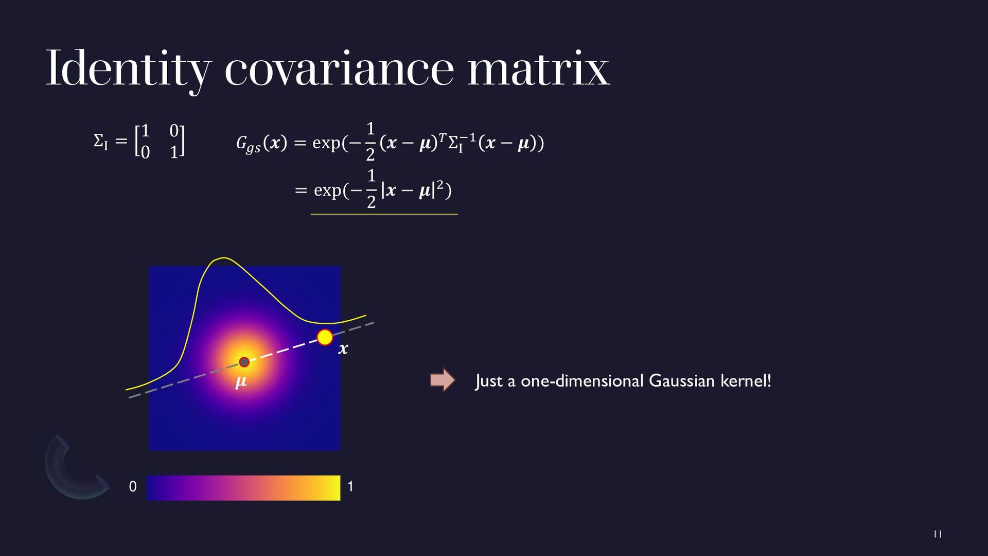
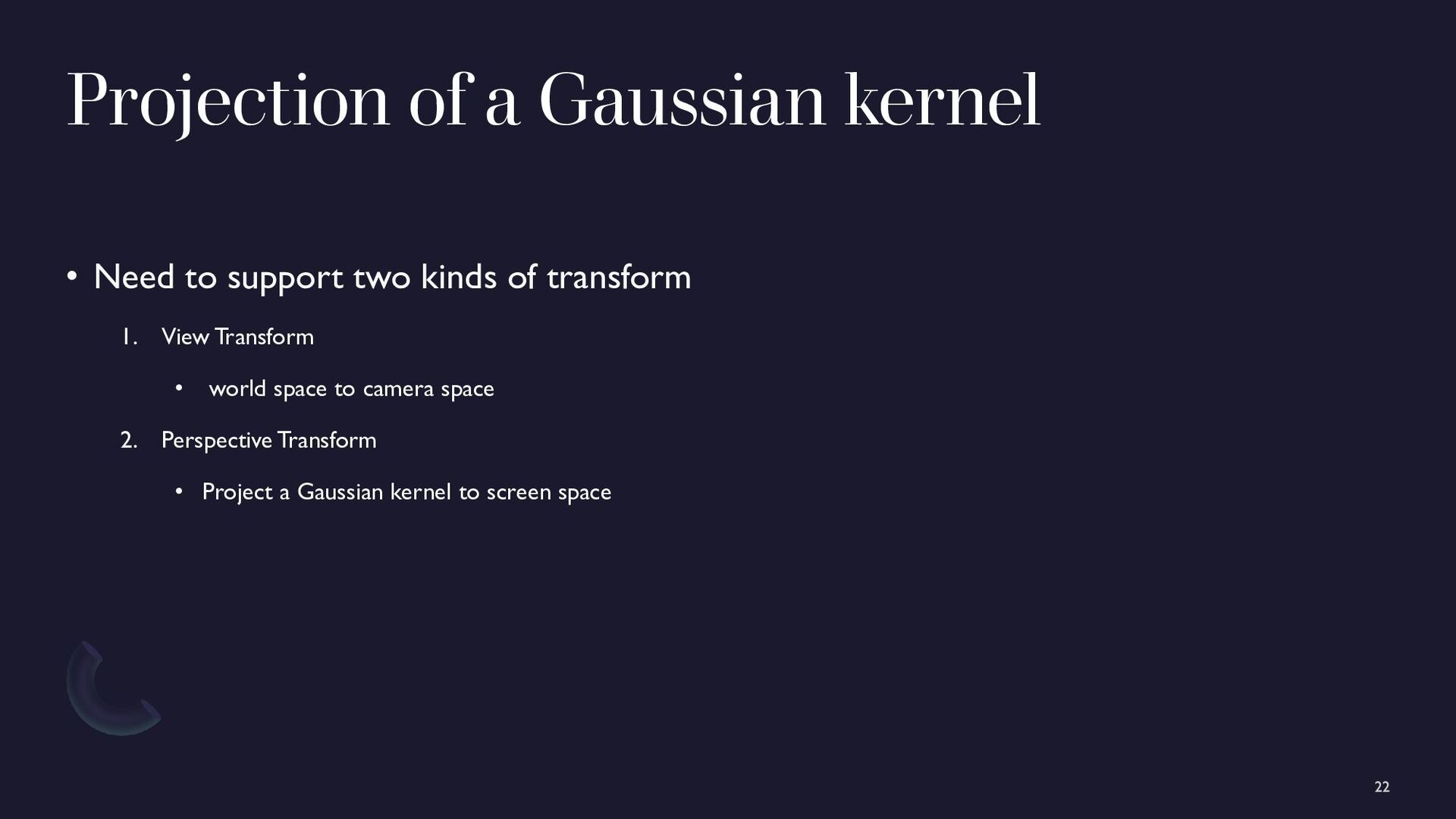
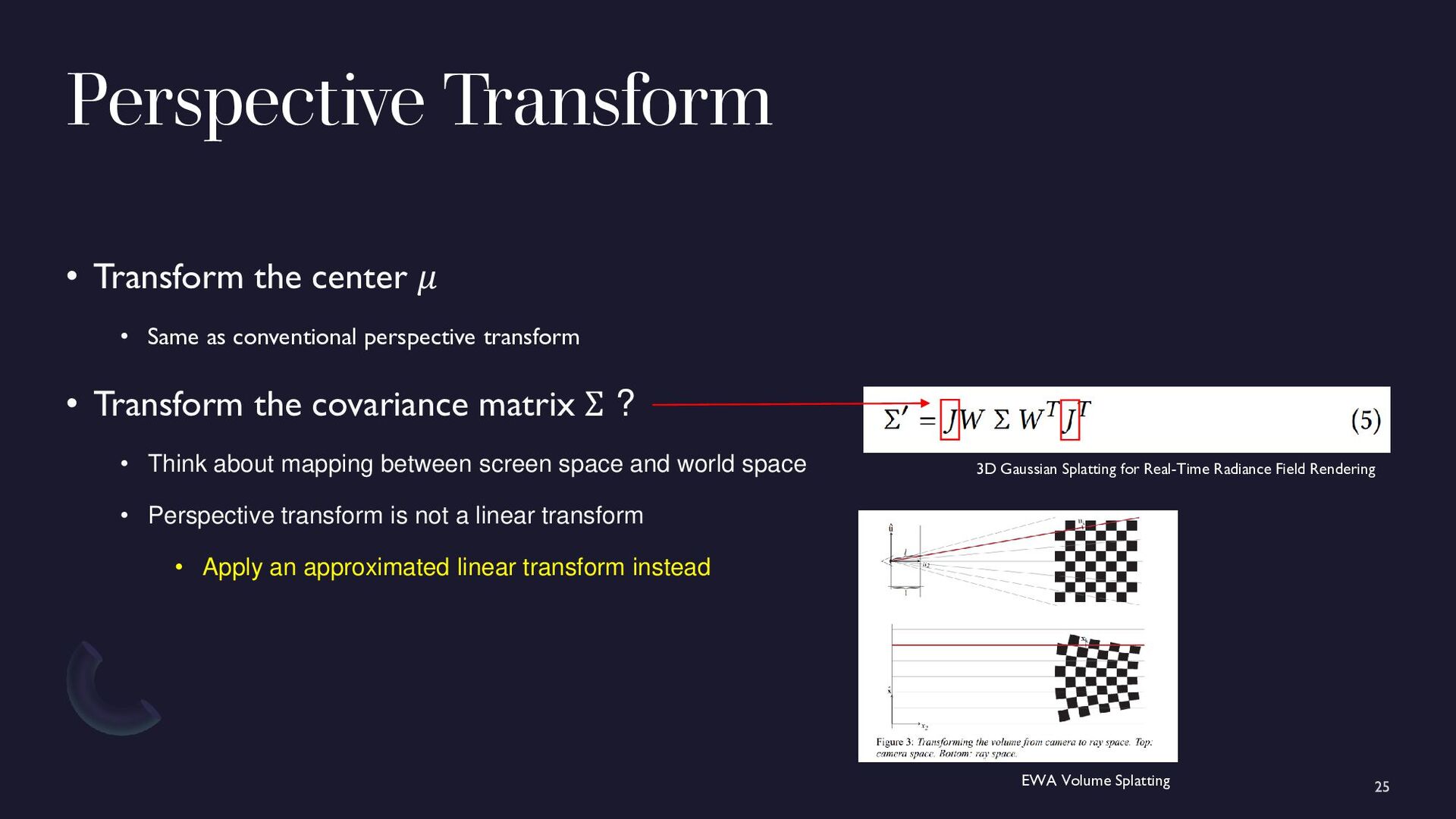
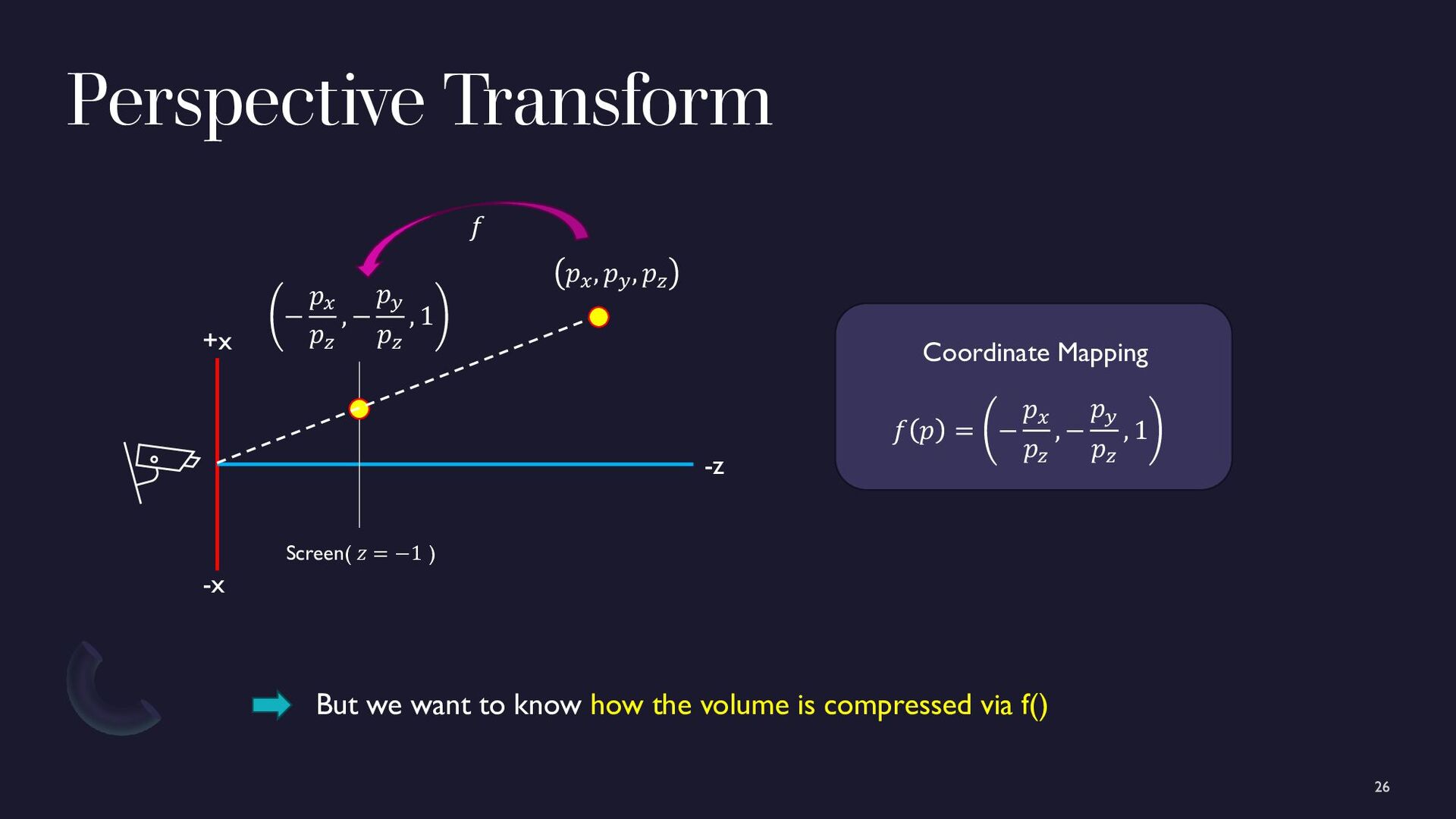
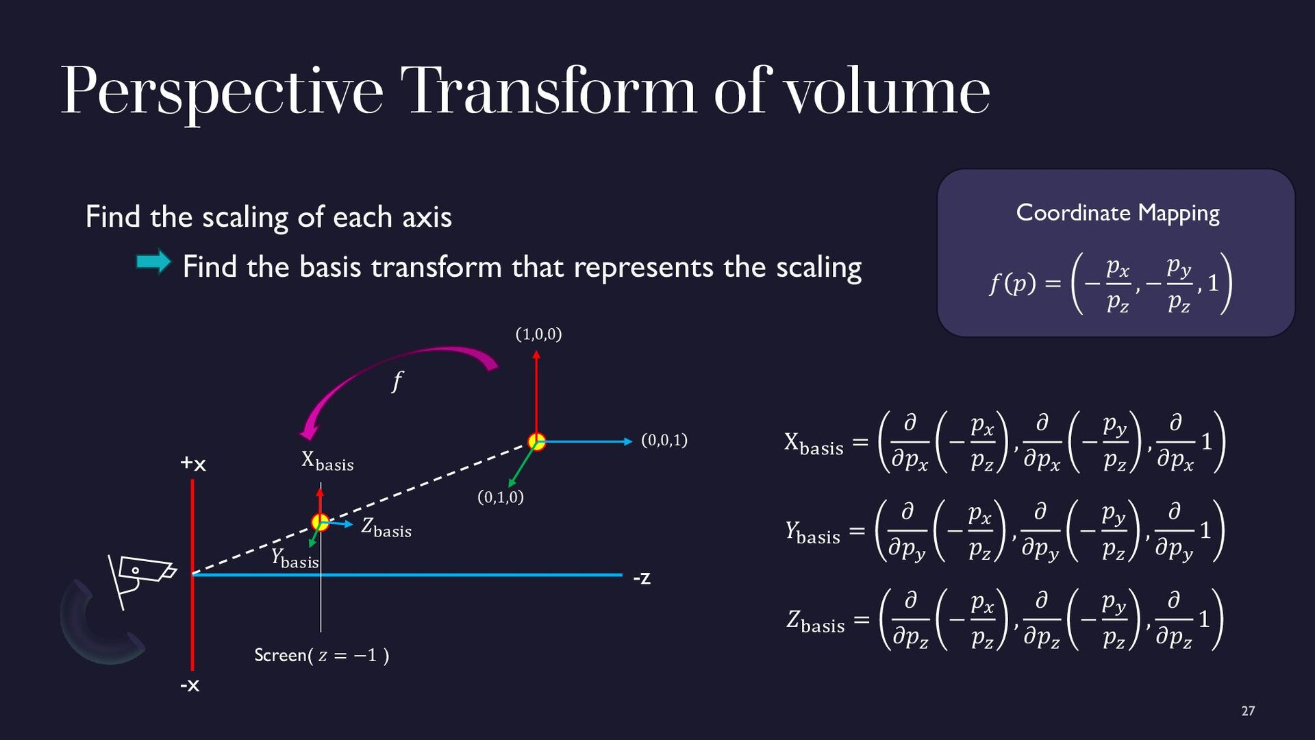
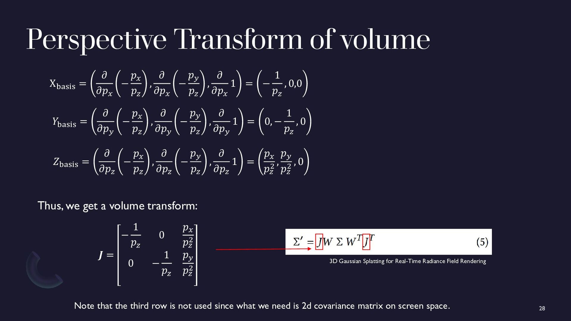
25. Perspective Transform • Transform the center 𝜇 • Same as conventional perspective transform • Transform the covariance matrix Σ ? • Think about mapping between screen space and world space • Perspective transform is not a linear transform • Apply an approximated linear transform instead 3D Gaussian Splatting for Real-Time Radiance Field Rendering EWA Volume Splatting
26. Perspective Transform Screen( 𝑧 = −1 ) -z +x -x − 𝑝𝑥 𝑝𝑧 , − 𝑝𝑦 𝑝𝑧 , 1 𝑝𝑥 , 𝑝𝑦 , 𝑝𝑧 𝑓 But we want to know how the volume is compressed via f() 𝑓 𝑝 = − 𝑝𝑥 𝑝𝑧 , − 𝑝𝑦 𝑝𝑧 , 1 Coordinate Mapping
27. Perspective Transform of volume Screen( 𝑧 = −1 ) -z +x -x 1,0,0 0,1,0 0,0,1 𝑓 Find the scaling of each axis Xbasis = 𝜕 𝜕𝑝𝑥 − 𝑝𝑥 𝑝𝑧 , 𝜕 𝜕𝑝𝑥 − 𝑝𝑦 𝑝𝑧 , 𝜕 𝜕𝑝𝑥 1 Find the basis transform that represents the scaling 𝑓 𝑝 = − 𝑝𝑥 𝑝𝑧 , − 𝑝𝑦 𝑝𝑧 , 1 Coordinate Mapping 𝑌basis = 𝜕 𝜕𝑝𝑦 − 𝑝𝑥 𝑝𝑧 , 𝜕 𝜕𝑝𝑦 − 𝑝𝑦 𝑝𝑧 , 𝜕 𝜕𝑝𝑦 1 𝑍basis = 𝜕 𝜕𝑝𝑧 − 𝑝𝑥 𝑝𝑧 , 𝜕 𝜕𝑝𝑧 − 𝑝𝑦 𝑝𝑧 , 𝜕 𝜕𝑝𝑧 1 Xbasis 𝑌basis 𝑍basis
28. Perspective Transform of volume Xbasis = 𝜕 𝜕𝑝𝑥 − 𝑝𝑥 𝑝𝑧 , 𝜕 𝜕𝑝𝑥 − 𝑝𝑦 𝑝𝑧 , 𝜕 𝜕𝑝𝑥 1 = − 1 𝑝𝑧 , 0,0 𝑌basis = 𝜕 𝜕𝑝𝑦 − 𝑝𝑥 𝑝𝑧 , 𝜕 𝜕𝑝𝑦 − 𝑝𝑦 𝑝𝑧 , 𝜕 𝜕𝑝𝑦 1 = 0, − 1 𝑝𝑧 , 0 𝑍basis = 𝜕 𝜕𝑝𝑧 − 𝑝𝑥 𝑝𝑧 , 𝜕 𝜕𝑝𝑧 − 𝑝𝑦 𝑝𝑧 , 𝜕 𝜕𝑝𝑧 1 = 𝑝𝑥 𝑝𝑧 2 , 𝑝𝑦 𝑝𝑧 2 , 0 Thus, we get a volume transform: 𝑱 = − 1 𝑝𝑧 0 𝑝𝑥 𝑝𝑧 2 0 − 1 𝑝𝑧 𝑝𝑦 𝑝𝑧 2 3D Gaussian Splatting for Real-Time Radiance Field Rendering Note that the third row is not used since what we need is 2d covariance matrix on screen space.
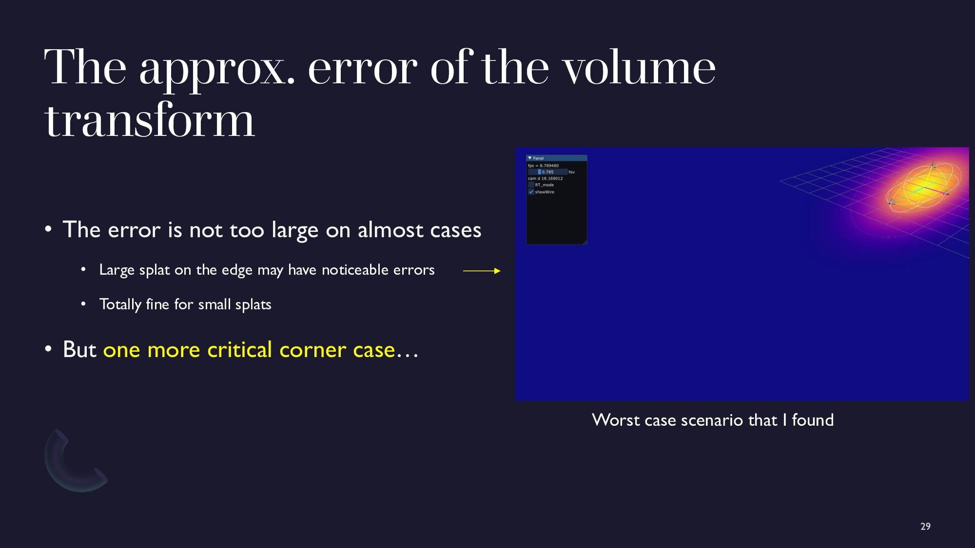
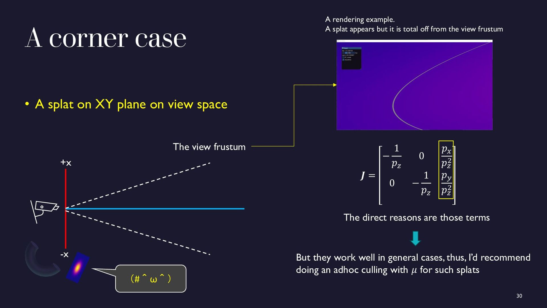
29. The approx. error of the volume transform • The error is not too large on almost cases • Large splat on the edge may have noticeable errors • Totally fine for small splats • But one more critical corner case… Worst case scenario that I found
30. A corner case • A splat on XY plane on view space +x -x （#＾ω＾） 𝑱 = − 1 𝑝𝑧 0 𝑝𝑥 𝑝𝑧 2 0 − 1 𝑝𝑧 𝑝𝑦 𝑝𝑧 2 The direct reasons are those terms But they work well in general cases, thus, I’d recommend doing an adhoc culling with 𝜇 for such splats The view frustum A rendering example. A splat appears but it is total off from the view frustum
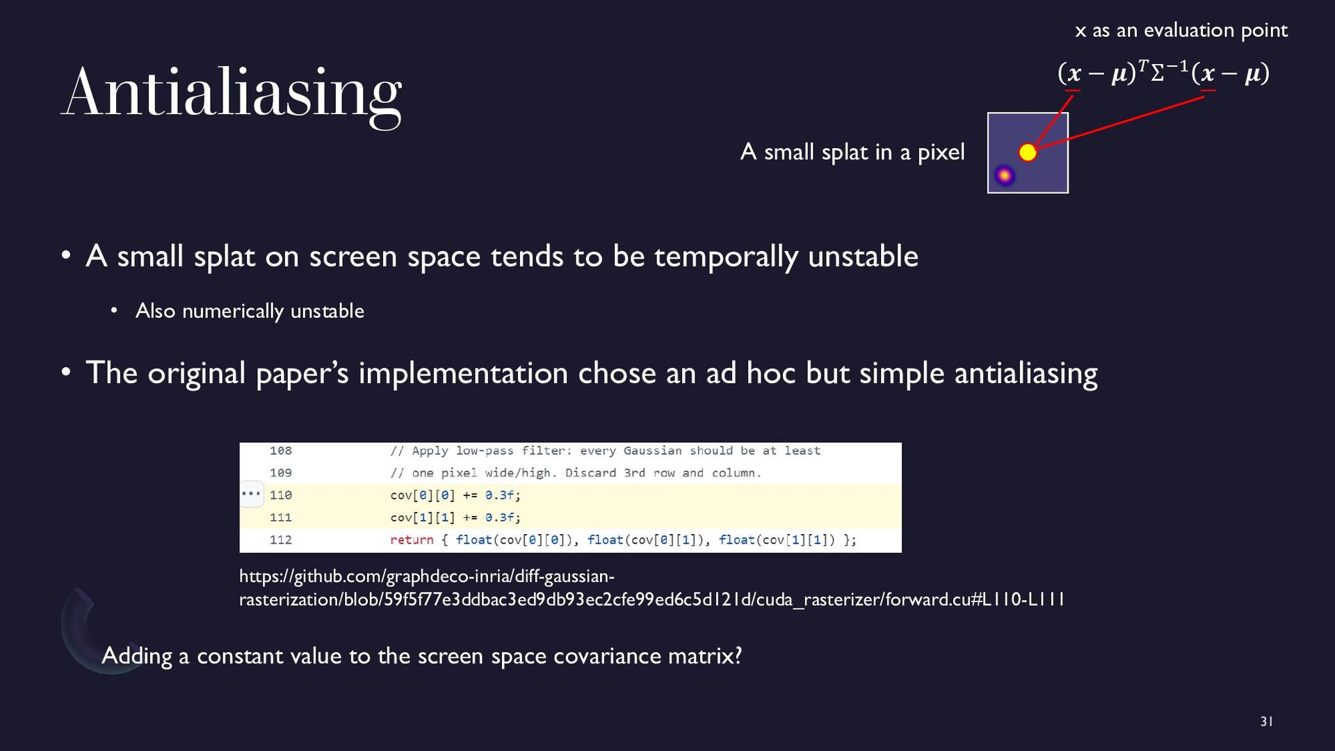
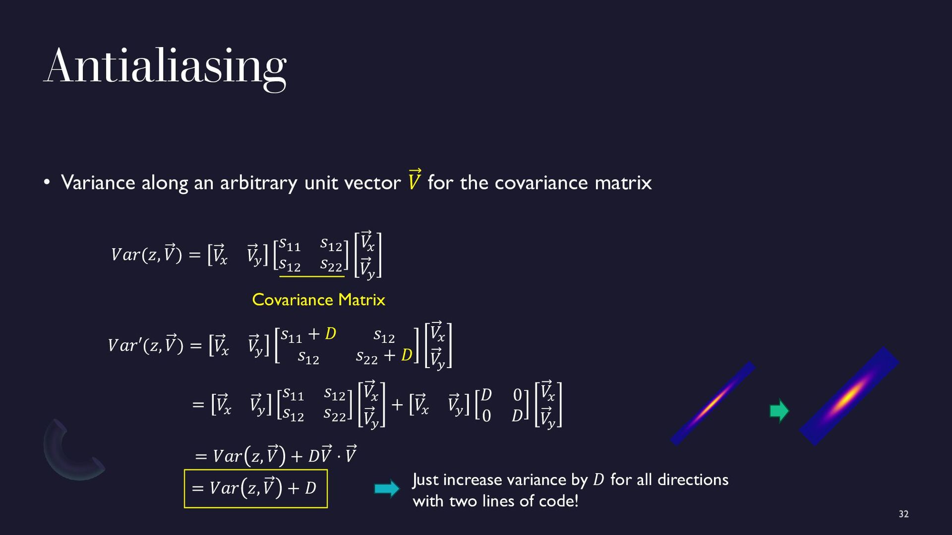
31. Antialiasing • A small splat on screen space tends to be temporally unstable • Also numerically unstable • The original paper’s implementation chose an ad hoc but simple antialiasing A small splat in a pixel 𝒙 − 𝝁 𝑇Σ−1 𝒙 − 𝝁 x as an evaluation point https://github.com/graphdeco-inria/diff-gaussian- rasterization/blob/59f5f77e3ddbac3ed9db93ec2cfe99ed6c5d121d/cuda_rasterizer/forward.cu#L110-L111 Adding a constant value to the screen space covariance matrix?
32. Antialiasing • Variance along an arbitrary unit vector 𝑉 for the covariance matrix 𝑉𝑎𝑟(𝑧, 𝑉) = 𝑉 𝑥 𝑉 𝑦 𝑠11 𝑠12 𝑠12 𝑠22 𝑉 𝑥 𝑉 𝑦 Covariance Matrix 𝑉𝑎𝑟′(𝑧, 𝑉) = 𝑉 𝑥 𝑉 𝑦 𝑠11 + 𝐷 𝑠12 𝑠12 𝑠22 + 𝐷 𝑉 𝑥 𝑉 𝑦 = 𝑉 𝑥 𝑉 𝑦 𝑠11 𝑠12 𝑠12 𝑠22 𝑉 𝑥 𝑉 𝑦 + 𝑉 𝑥 𝑉 𝑦 𝐷 0 0 𝐷 𝑉 𝑥 𝑉 𝑦 = 𝑉𝑎𝑟 𝑧, 𝑉 + 𝐷𝑉 ⋅ 𝑉 = 𝑉𝑎𝑟 𝑧, 𝑉 + 𝐷 Just increase variance by 𝐷 for all directions with two lines of code!
33. GPU Implementation
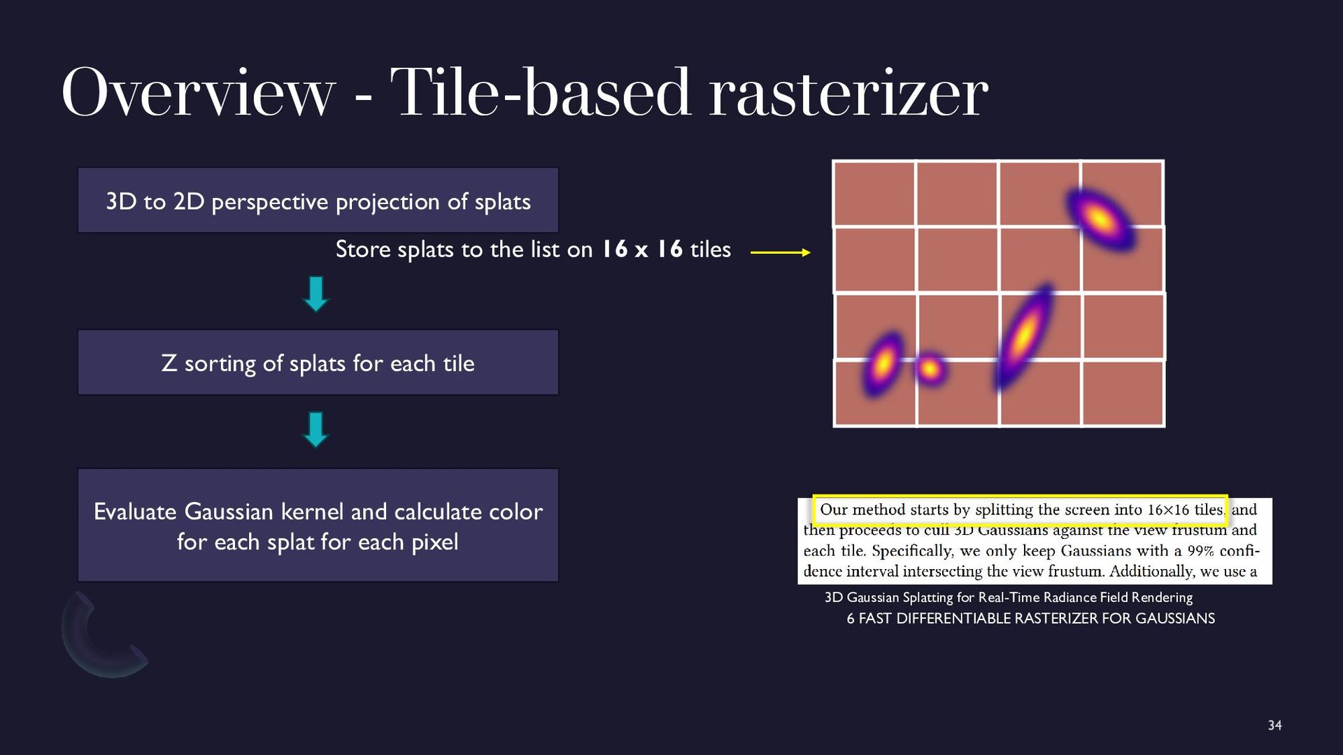
34. Overview - Tile-based rasterizer Z sorting of splats for each tile Evaluate Gaussian kernel and calculate color for each splat for each pixel 6 FAST DIFFERENTIABLE RASTERIZER FOR GAUSSIANS 3D Gaussian Splatting for Real-Time Radiance Field Rendering 3D to 2D perspective projection of splats Store splats to the list on 16 x 16 tiles
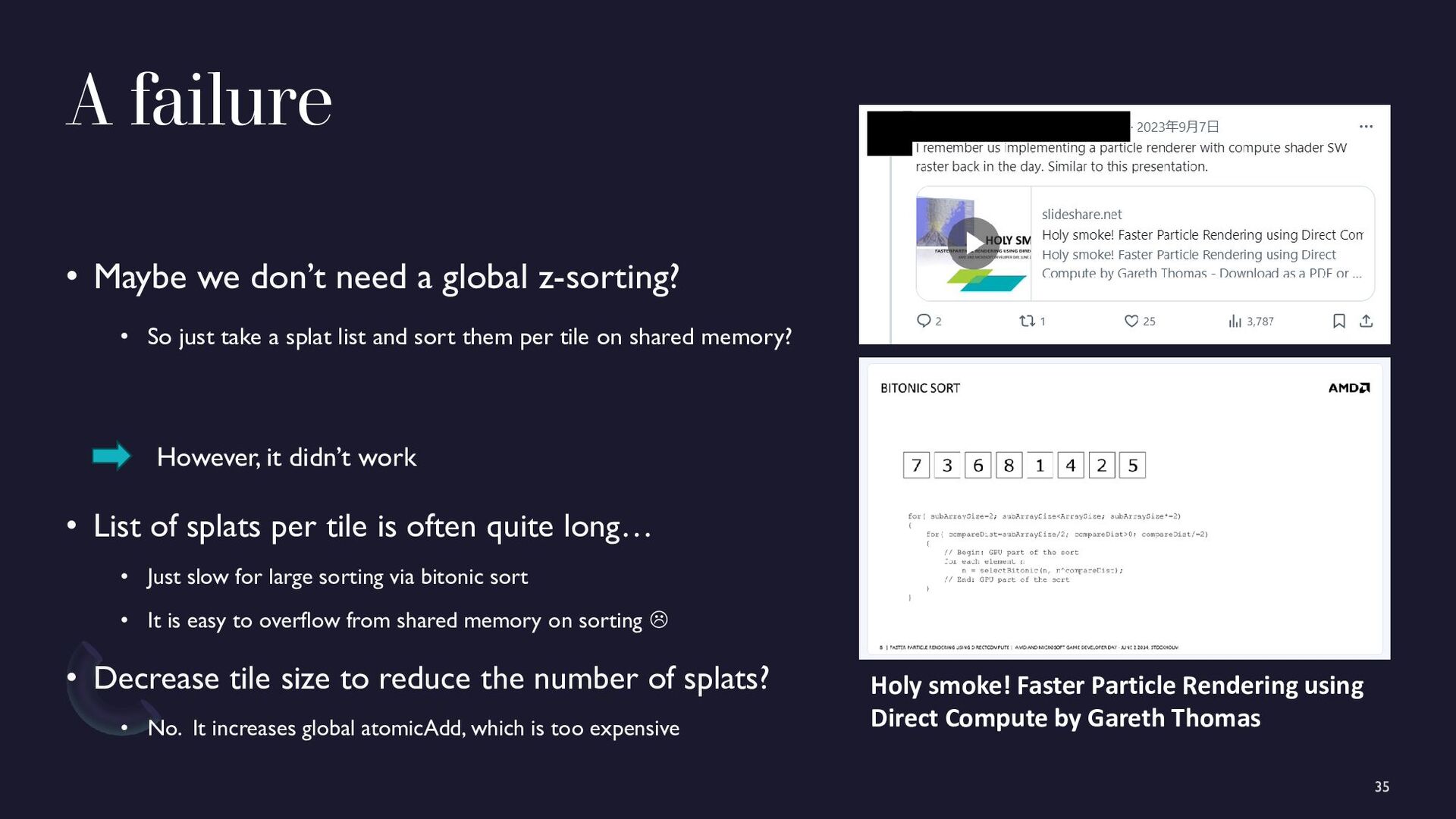
35. A failure • Maybe we don’t need a global z-sorting? • So just take a splat list and sort them per tile on shared memory? Holy smoke! Faster Particle Rendering using Direct Compute by Gareth Thomas However, it didn’t work • List of splats per tile is often quite long… • Just slow for large sorting via bitonic sort • It is easy to overflow from shared memory on sorting  • Decrease tile size to reduce the number of splats? • No. It increases global atomicAdd, which is too expensive
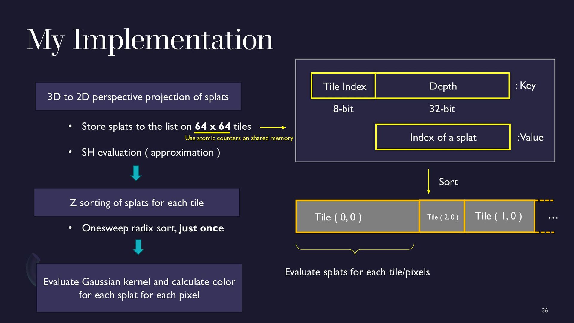
36. My Implementation 3D to 2D perspective projection of splats • Store splats to the list on 64 x 64 tiles • SH evaluation ( approximation ) Z sorting of splats for each tile • Onesweep radix sort, just once Tile Index Depth 8-bit 32-bit Index of a splat : Key : Value Tile ( 0, 0 ) Tile ( 1, 0 ) Tile ( 2, 0 ) … Sort Evaluate Gaussian kernel and calculate color for each splat for each pixel Evaluate splats for each tile/pixels Use atomic counters on shared memory
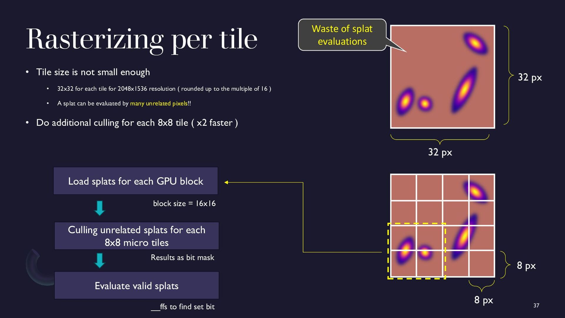
37. Rasterizing per tile • Tile size is not small enough • 32x32 for each tile for 2048x1536 resolution ( rounded up to the multiple of 16 ) • A splat can be evaluated by many unrelated pixels!! • Do additional culling for each 8x8 tile ( x2 faster ) 32 px 32 px Waste of splat evaluations 8 px 8 px Load splats for each GPU block block size = 16x16 Culling unrelated splats for each 8x8 micro tiles Results as bit mask Evaluate valid splats __ffs to find set bit
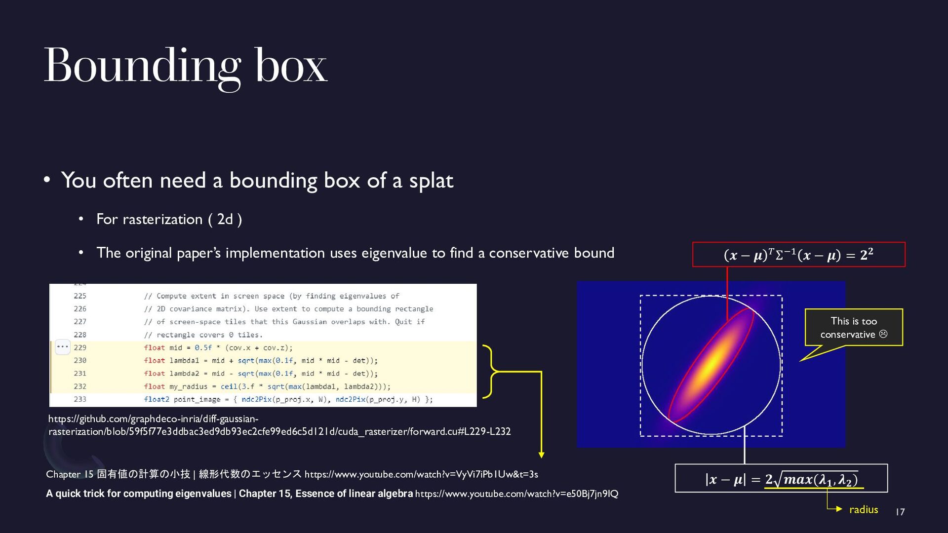
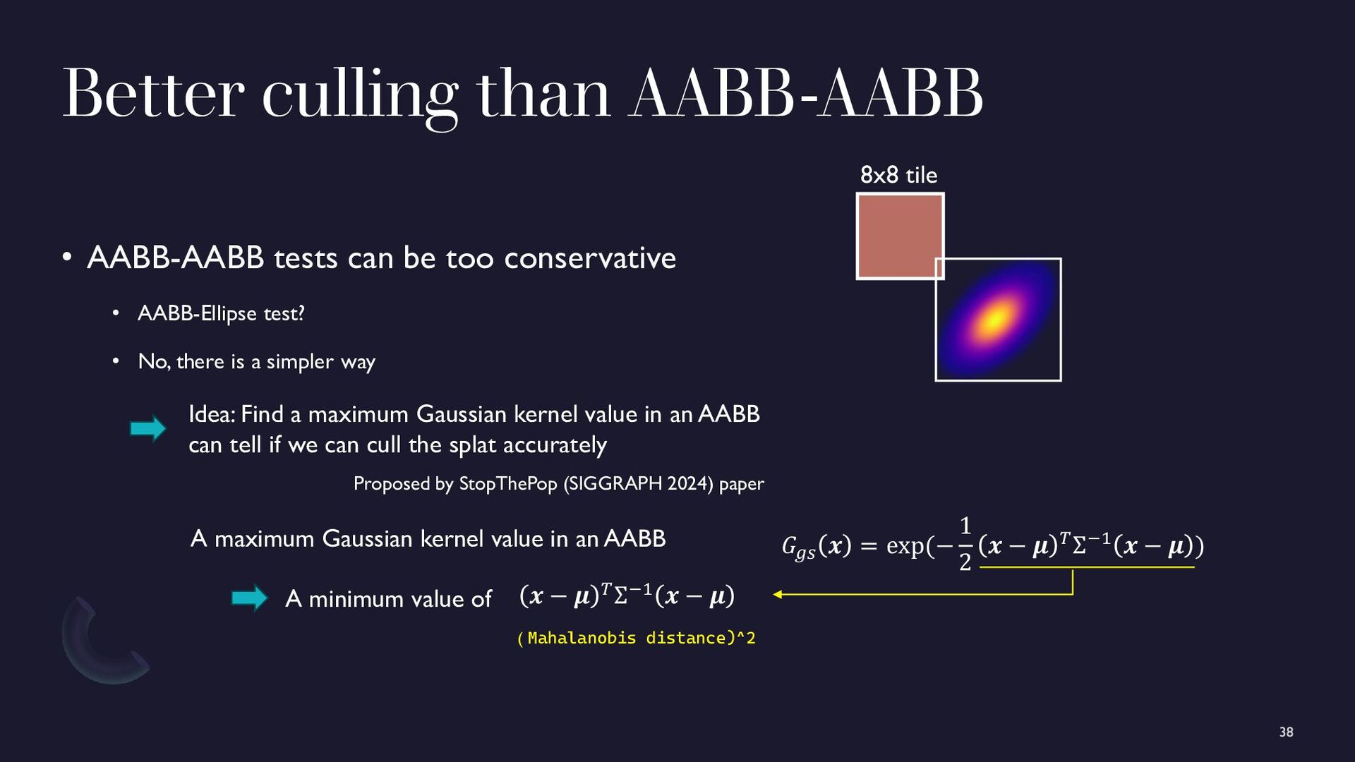
38. Better culling than AABB-AABB • AABB-AABB tests can be too conservative • AABB-Ellipse test? • No, there is a simpler way 8x8 tile Idea: Find a maximum Gaussian kernel value in an AABB can tell if we can cull the splat accurately Proposed by StopThePop (SIGGRAPH 2024) paper A maximum Gaussian kernel value in an AABB 𝒙 − 𝝁 𝑇Σ−1 𝒙 − 𝝁 A minimum value of 𝐺𝑔𝑠 𝒙 = exp(− 1 2 𝒙 − 𝝁 𝑇Σ−1 𝒙 − 𝝁 ) ( Mahalanobis distance)^2
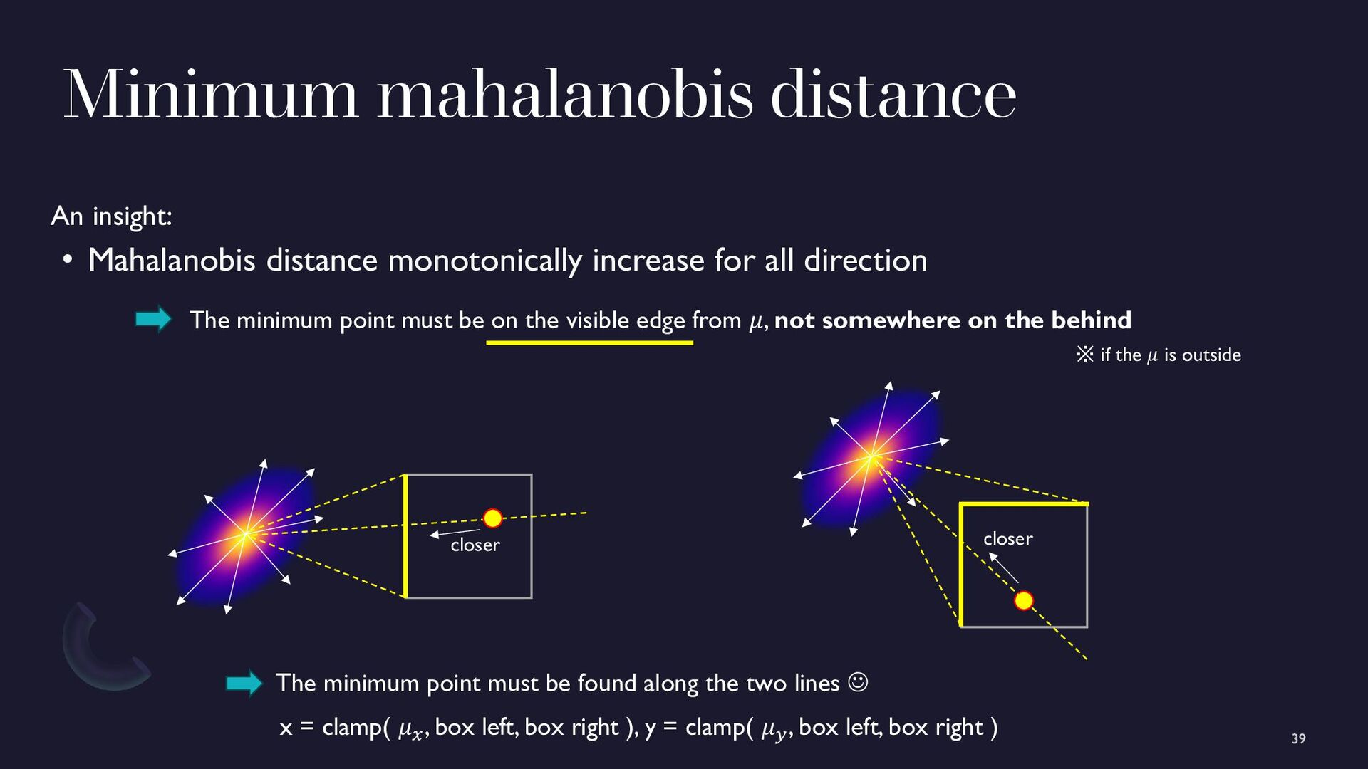
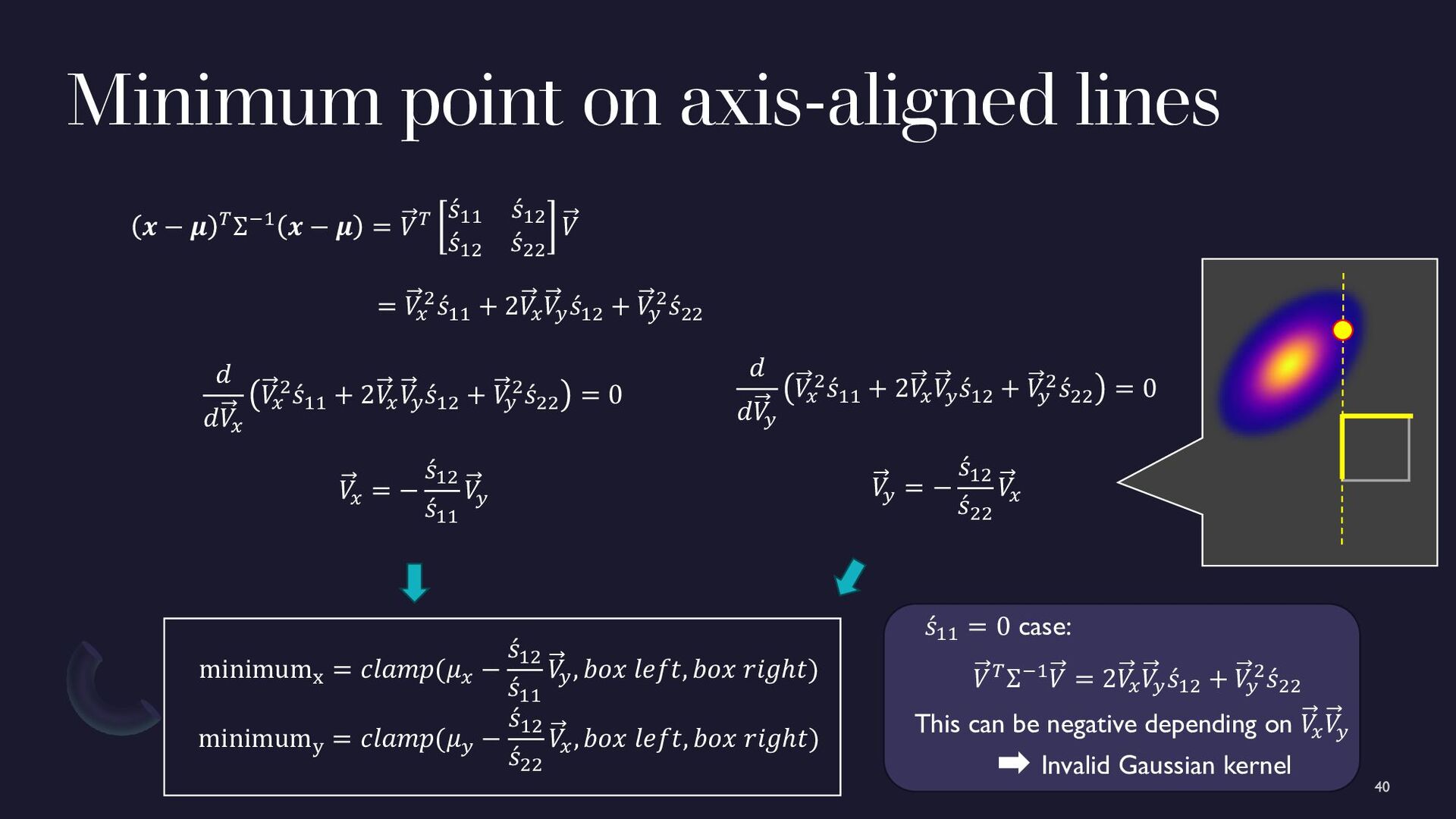
39. Minimum mahalanobis distance • Mahalanobis distance monotonically increase for all direction closer An insight: The minimum point must be found along the two lines ☺ x = clamp( 𝜇𝑥, box left, box right ), y = clamp( 𝜇𝑦, box left, box right ) The minimum point must be on the visible edge from 𝜇, not somewhere on the behind ※ if the 𝜇 is outside closer
40. Minimum point on axis-aligned lines 𝒙 − 𝝁 𝑇Σ−1 𝒙 − 𝝁 = 𝑉𝑇 ƴ 𝑠11 ƴ 𝑠12 ƴ 𝑠12 ƴ 𝑠22 𝑉 = 𝑉 𝑥 2 ƴ 𝑠11 + 2𝑉 𝑥 𝑉 𝑦 ƴ 𝑠12 + 𝑉 𝑦 2 ƴ 𝑠22 𝑉 𝑥 = − ƴ 𝑠12 ƴ 𝑠11 𝑉 𝑦 𝑉 𝑦 = − ƴ 𝑠12 ƴ 𝑠22 𝑉 𝑥 𝑑 𝑑𝑉 𝑥 𝑉 𝑥 2 ƴ 𝑠11 + 2𝑉 𝑥 𝑉 𝑦 ƴ 𝑠12 + 𝑉 𝑦 2 ƴ 𝑠22 = 0 𝑑 𝑑𝑉 𝑦 𝑉 𝑥 2 ƴ 𝑠11 + 2𝑉 𝑥 𝑉 𝑦 ƴ 𝑠12 + 𝑉 𝑦 2 ƴ 𝑠22 = 0 minimumx = 𝑐𝑙𝑎𝑚𝑝(𝜇𝑥 − ƴ 𝑠12 ƴ 𝑠11 𝑉 𝑦 , 𝑏𝑜𝑥 𝑙𝑒𝑓𝑡, 𝑏𝑜𝑥 𝑟𝑖𝑔ℎ𝑡) minimumy = 𝑐𝑙𝑎𝑚𝑝(𝜇𝑦 − ƴ 𝑠12 ƴ 𝑠22 𝑉 𝑥 , 𝑏𝑜𝑥 𝑙𝑒𝑓𝑡, 𝑏𝑜𝑥 𝑟𝑖𝑔ℎ𝑡) ƴ 𝑠11 = 0 case: 𝑉𝑇Σ−1𝑉 = 2𝑉 𝑥 𝑉 𝑦 ƴ 𝑠12 + 𝑉 𝑦 2 ƴ 𝑠22 This can be negative depending on 𝑉 𝑥 𝑉 𝑦 Invalid Gaussian kernel
41. RX 7900 XTX RealTime
42. Conclusion • Introduced the Gaussian splatting formulation in intuitive ways • Easy to control its behavior • Can be optimized by a simple idea/formula • GPU implementation • The white-box splat representation helps to optimize the implementation on the GPU too • Thank you, linear algebra
43. References • 3D Gaussian Splatting for Real-Time Radiance Field Rendering • EWA Volume Splatting • A geometric interpretation of the covariance matrix • Holy smoke! Faster Particle Rendering using Direct Compute by Gareth Thomas • 驚くほどキレイな三次元シーン復元、「3D Gaussian Splatting」を徹底的に解説 する
44. で、レイトレは？