Language Modelling, from Natural Language Processing by Jurafsky&Manning at Coursera

Transcript

1.   Introduc*on  to  N-­‐grams       Language   Modeling  
2. Dan  Jurafsky   Probabilis1c  Language  Models   •  Today’s  goal:  assign  a  probability  to  a  sentence   •  Machine  Transla*on:   •  P(high  winds  tonite)  >  P(large  winds  tonite)   •  Spell  Correc*on   •  The  office  is  about  fiIeen  minuets  from  my  house   •  P(about  fiIeen  minutes  from)  >  P(about  fiIeen  minuets  from)   •  Speech  Recogni*on   •  P(I  saw  a  van)  >>  P(eyes  awe  of  an)   •  +  Summariza*on,  ques*on-­‐answering,  etc.,  etc.!!   Why?  
3. Dan  Jurafsky   Probabilis1c  Language  Modeling   •  Goal:  compute  the  probability  of  a  sentence  or   sequence  of  words:            P(W)  =  P(w1 ,w2 ,w3 ,w4 ,w5 …wn )   •  Related  task:  probability  of  an  upcoming  word:              P(w5 |w1 ,w2 ,w3 ,w4 )   •  A  model  that  computes  either  of  these:                      P(W)          or          P(wn |w1 ,w2 …wn-­‐1 )                    is  called  a  language  model.   •  Be_er:  the  grammar              But  language  model  or  LM  is  standard  
4. Dan  Jurafsky   How  to  compute  P(W)   •  How  to  compute  this  joint  probability:   •  P(its,  water,  is,  so,  transparent,  that)   •  Intui*on:  let’s  rely  on  the  Chain  Rule  of  Probability  
5. Dan  Jurafsky   Reminder:  The  Chain  Rule   •  Recall  the  defini*on  of  condi*onal  probabili*es                  Rewri*ng:     •  More  variables:    P(A,B,C,D)  =  P(A)P(B|A)P(C|A,B)P(D|A,B,C)   •  The  Chain  Rule  in  General      P(x1 ,x2 ,x3 ,…,xn )  =  P(x1 )P(x2 |x1 )P(x3 |x1 ,x2 )…P(xn |x1 ,…,xn-­‐1 )    
6. Dan  Jurafsky   The  Chain  Rule  applied  to  compute   joint  probability  of  words  in  sentence         P(“its  water  is  so  transparent”)  =    P(its)  ×  P(water|its)  ×    P(is|its  water)                      ×    P(so|its  water  is)  ×    P(transparent|its  water  is  so)   ! P(w 1 w 2 …w n ) = P(w i | w 1 w 2 …w i"1 ) i #
7. Dan  Jurafsky   How  to  es1mate  these  probabili1es   •  Could  we  just  count  and  divide?   •  No!    Too  many  possible  sentences!   •  We’ll  never  see  enough  data  for  es*ma*ng  these   ! P(the |its water is so transparent that) = Count(its water is so transparent that the) Count(its water is so transparent that)
8. Dan  Jurafsky   Markov  Assump1on   •  Simplifying  assump*on:       •  Or  maybe     P(the |its water is so transparent that) " P(the |that) P(the |its water is so transparent that) " P(the |transparent that) Andrei  Markov  
9. Dan  Jurafsky   Markov  Assump1on   •  In  other  words,  we  approximate  each   component  in  the  product     P(w 1 w 2 …w n ) " P(w i | w i#k …w i#1 ) i $ P(w i | w 1 w 2 …w i"1 ) # P(w i | w i"k …w i"1 )
10. Dan  Jurafsky   Simplest  case:  Unigram  model   fifth, an, of, futures, the, an, incorporated, a, a, the, inflation, most, dollars, quarter, in, is, mass! ! thrift, did, eighty, said, hard, 'm, july, bullish! ! that, or, limited, the! Some  automa*cally  generated  sentences  from  a  unigram  model   ! P(w 1 w 2 …w n ) " P(w i ) i #
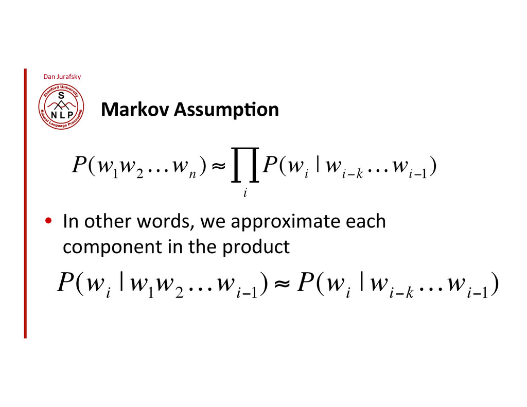
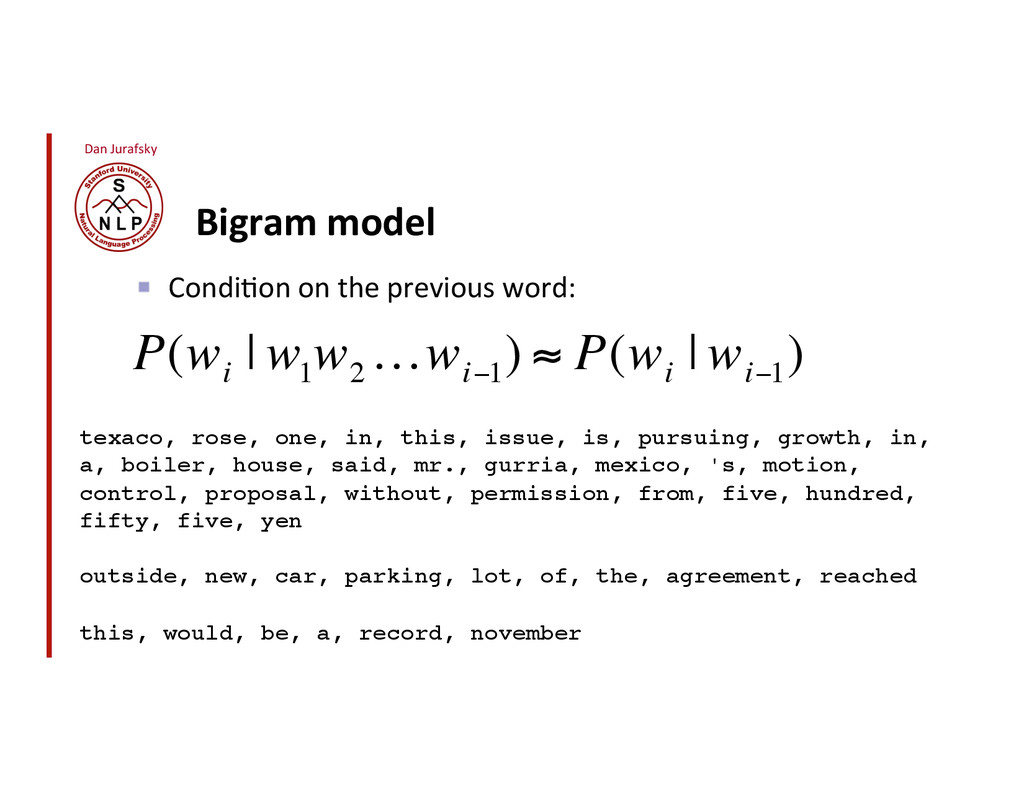
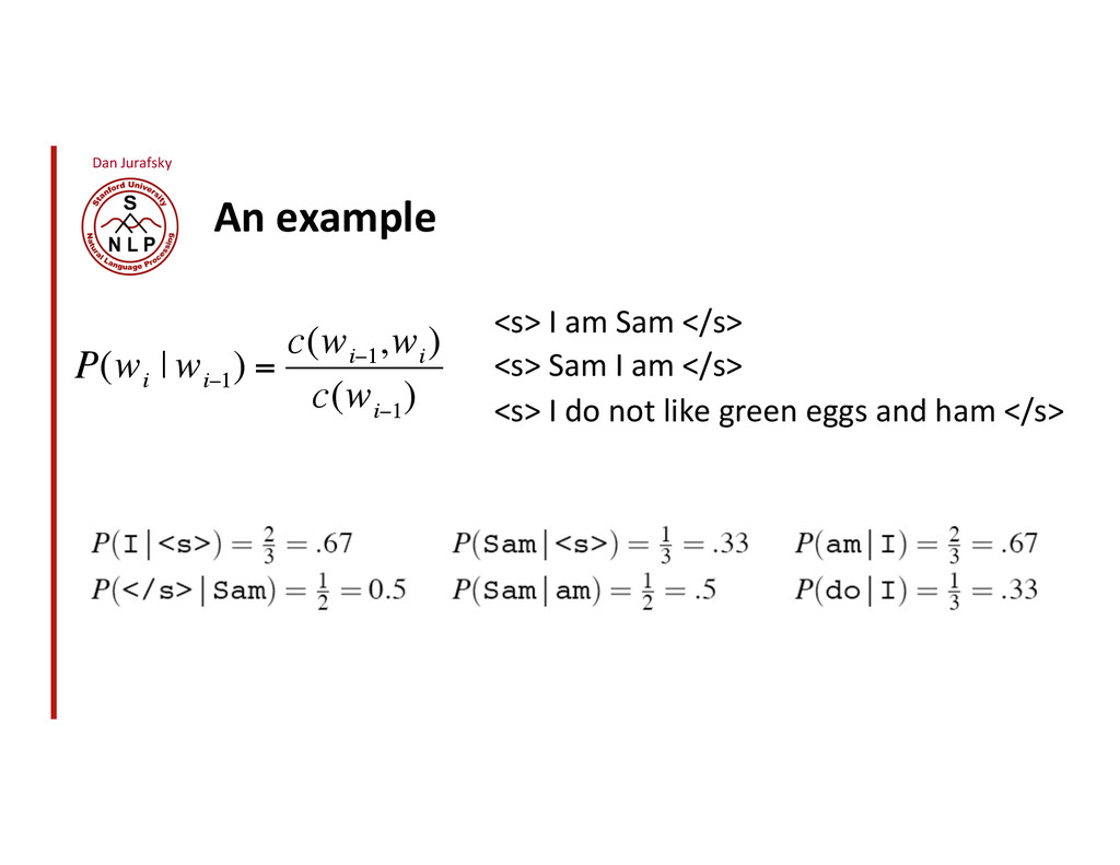
11. Dan  Jurafsky   " Condi*on  on  the  previous  word:   Bigram  model   texaco, rose, one, in, this, issue, is, pursuing, growth, in, a, boiler, house, said, mr., gurria, mexico, 's, motion, control, proposal, without, permission, from, five, hundred, fifty, five, yen! ! outside, new, car, parking, lot, of, the, agreement, reached! ! this, would, be, a, record, november! P(w i | w 1 w 2 …w i"1 ) # P(w i | w i"1 )
12. Dan  Jurafsky   N-­‐gram  models   •  We  can  extend  to  trigrams,  4-­‐grams,  5-­‐grams   •  In  general  this  is  an  insufficient  model  of  language   •  because  language  has  long-­‐distance  dependencies:     “The  computer  which  I  had  just  put  into  the  machine  room  on   the  fiIh  floor  crashed.”   •  But  we  can  oIen  get  away  with  N-­‐gram  models  
13.   Introduc*on  to  N-­‐grams       Language   Modeling  
14.   Es*ma*ng  N-­‐gram   Probabili*es       Language   Modeling  
15. Dan  Jurafsky   Es1ma1ng  bigram  probabili1es   •  The  Maximum  Likelihood  Es*mate   ! P(w i | w i"1 ) = count(w i"1 ,w i ) count(w i"1 ) P(w i | w i"1 ) = c(w i"1 ,w i ) c(w i"1 )
16. Dan  Jurafsky   An  example   <s>  I  am  Sam  </s>   <s>  Sam  I  am  </s>   <s>  I  do  not  like  green  eggs  and  ham  </s>     P(w i | w i"1 ) = c(w i"1 ,w i ) c(w i"1 )
17. Dan  Jurafsky   More  examples:     Berkeley  Restaurant  Project  sentences   •  can  you  tell  me  about  any  good  cantonese  restaurants  close  by   •  mid  priced  thai  food  is  what  i’m  looking  for   •  tell  me  about  chez  panisse   •  can  you  give  me  a  lis*ng  of  the  kinds  of  food  that  are  available   •  i’m  looking  for  a  good  place  to  eat  breakfast   •  when  is  caffe  venezia  open  during  the  day
18. Dan  Jurafsky   Raw  bigram  counts   •  Out  of  9222  sentences  
19. Dan  Jurafsky   Raw  bigram  probabili1es   •  Normalize  by  unigrams:   •  Result:  
20. Dan  Jurafsky   Bigram  es1mates  of  sentence  probabili1es   P(<s>  I  want  english  food  </s>)  =    P(I|<s>)            ×    P(want|I)        ×    P(english|want)          ×    P(food|english)          ×    P(</s>|food)                =    .000031  
21. Dan  Jurafsky   What  kinds  of  knowledge?   •  P(english|want)    =  .0011   •  P(chinese|want)  =    .0065   •  P(to|want)  =  .66   •  P(eat  |  to)  =  .28   •  P(food  |  to)  =  0   •  P(want  |  spend)  =  0   •  P  (i  |  <s>)  =  .25  
22. Dan  Jurafsky   Prac1cal  Issues   •  We  do  everything  in  log  space   • Avoid  underflow   • (also  adding  is  faster  than  mul*plying)   log(p1 ! p2 ! p3 ! p4 ) = log p1 + log p2 + log p3 + log p4
23. Dan  Jurafsky   Language  Modeling  Toolkits   •  SRILM   • h_p://www.speech.sri.com/projects/srilm/  
24. Dan  Jurafsky   Google  N-­‐Gram  Release,  August  2006   …
25. Dan  Jurafsky   Google  N-­‐Gram  Release   •  serve as the incoming 92! •  serve as the incubator 99! •  serve as the independent 794! •  serve as the index 223! •  serve as the indication 72! •  serve as the indicator 120! •  serve as the indicators 45! •  serve as the indispensable 111! •  serve as the indispensible 40! •  serve as the individual 234! http://googleresearch.blogspot.com/2006/08/all-our-n-gram-are-belong-to-you.html
26. Dan  Jurafsky   Google  Book  N-­‐grams   •  h_p://ngrams.googlelabs.com/  
27.   Es*ma*ng  N-­‐gram   Probabili*es       Language   Modeling  
28.   Evalua*on  and   Perplexity       Language   Modeling  
29. Dan  Jurafsky   Evalua1on:  How  good  is  our  model?   •  Does  our  language  model  prefer  good  sentences  to  bad  ones?   •  Assign  higher  probability  to  “real”  or  “frequently  observed”  sentences     •  Than  “ungramma*cal”  or  “rarely  observed”  sentences?   •  We  train  parameters  of  our  model  on  a  training  set.   •  We  test  the  model’s  performance  on  data  we  haven’t  seen.   •  A  test  set  is  an  unseen  dataset  that  is  different  from  our  training  set,   totally  unused.   •  An  evalua1on  metric  tells  us  how  well  our  model  does  on  the  test  set.  
30. Dan  Jurafsky   Extrinsic  evalua1on  of  N-­‐gram  models   •  Best  evalua*on  for  comparing  models  A  and  B   •  Put  each  model  in  a  task   •   spelling  corrector,  speech  recognizer,  MT  system   •  Run  the  task,  get  an  accuracy  for  A  and  for  B   •  How  many  misspelled  words  corrected  properly   •  How  many  words  translated  correctly   •  Compare  accuracy  for  A  and  B  
31. Dan  Jurafsky   Difficulty  of  extrinsic  (in-­‐vivo)  evalua1on  of     N-­‐gram  models   •  Extrinsic  evalua*on   •  Time-­‐consuming;  can  take  days  or  weeks   •  So   •  Some*mes  use  intrinsic  evalua*on:  perplexity   •  Bad  approxima*on     •  unless  the  test  data  looks  just  like  the  training  data   •  So  generally  only  useful  in  pilot  experiments   •  But  is  helpful  to  think  about.  
32. Dan  Jurafsky   Intui1on  of  Perplexity   •  The  Shannon  Game:   •  How  well  can  we  predict  the  next  word?   •  Unigrams  are  terrible  at  this  game.    (Why?)   •  A  be_er  model  of  a  text   •   is  one  which  assigns  a  higher  probability  to  the  word  that  actually  occurs   I  always  order  pizza  with  cheese  and  ____   The  33rd  President  of  the  US  was  ____   I  saw  a  ____   mushrooms 0.1 pepperoni 0.1 anchovies 0.01 …. fried rice 0.0001 …. and 1e-100
33. Dan  Jurafsky   Perplexity   Perplexity  is  the  inverse  probability  of   the  test  set,  normalized  by  the  number   of  words:                                                                                                Chain  rule:                                                                                                For  bigrams:   Minimizing  perplexity  is  the  same  as  maximizing  probability   The  best  language  model  is  one  that  best  predicts  an  unseen  test  set   •  Gives  the  highest  P(sentence)   PP(W) = P(w1 w2 ...wN ) ! 1 N = 1 P(w1 w2 ...wN ) N
34. Dan  Jurafsky   The  Shannon  Game  intui1on  for  perplexity   •  From  Josh  Goodman   •  How  hard  is  the  task  of  recognizing  digits  ‘0,1,2,3,4,5,6,7,8,9’   •  Perplexity  10   •  How  hard  is  recognizing  (30,000)  names  at  MicrosoI.     •  Perplexity  =  30,000   •  If  a  system  has  to  recognize   •  Operator  (1  in  4)   •  Sales  (1  in  4)   •  Technical  Support  (1  in  4)   •  30,000  names  (1  in  120,000  each)   •  Perplexity  is  53   •  Perplexity  is  weighted  equivalent  branching  factor  
35. Dan  Jurafsky   Perplexity  as  branching  factor   •  Let’s  suppose  a  sentence  consis*ng  of  random  digits   •  What  is  the  perplexity  of  this  sentence  according  to  a  model   that  assign  P=1/10  to  each  digit?  
36. Dan  Jurafsky   Lower  perplexity  =  beXer  model     •  Training  38  million  words,  test  1.5  million  words,  WSJ   N-­‐gram   Order   Unigram   Bigram   Trigram   Perplexity   962   170   109  
37.   Evalua*on  and   Perplexity       Language   Modeling  
38.   Generaliza*on  and   zeros       Language   Modeling  
39. Dan  Jurafsky   The  Shannon  Visualiza1on  Method   •  Choose  a  random  bigram              (<s>,  w)  according  to  its  probability   •  Now  choose  a  random  bigram                 (w,  x)  according  to  its  probability   •  And  so  on  un*l  we  choose  </s>   •  Then  string  the  words  together   <s> I! I want! want to! to eat! eat Chinese! Chinese food! food </s>! I want to eat Chinese food!
40. Dan  Jurafsky   Approxima1ng  Shakespeare      
41. Dan  Jurafsky   Shakespeare  as  corpus   •  N=884,647  tokens,  V=29,066   •  Shakespeare  produced  300,000  bigram  types   out  of  V2=  844  million  possible  bigrams.   •  So  99.96%  of  the  possible  bigrams  were  never  seen   (have  zero  entries  in  the  table)   •  Quadrigrams  worse:      What's  coming  out  looks   like  Shakespeare  because  it  is  Shakespeare  
42. Dan  Jurafsky   The  wall  street  journal  is  not  shakespeare   (no  offense)  
43. Dan  Jurafsky   The  perils  of  overfi]ng   •  N-­‐grams  only  work  well  for  word  predic*on  if  the  test   corpus  looks  like  the  training  corpus   •  In  real  life,  it  oIen  doesn’t   •  We  need  to  train  robust  models  that  generalize!   •  One  kind  of  generaliza*on:  Zeros!   •  Things  that  don’t  ever  occur  in  the  training  set   •  But  occur  in  the  test  set  
44. Dan  Jurafsky   Zeros •  Training  set:   …  denied  the  allega*ons   …  denied  the  reports   …  denied  the  claims   …  denied  the  request     P(“offer”  |  denied  the)  =  0 •  Test  set   …  denied  the  offer   …  denied  the  loan  
45. Dan  Jurafsky   Zero  probability  bigrams   •  Bigrams  with  zero  probability   •  mean  that  we  will  assign  0  probability  to  the  test  set!   •  And  hence  we  cannot  compute  perplexity  (can’t  divide  by  0)!  
46.   Generaliza*on  and   zeros       Language   Modeling  
47.   Smoothing:  Add-­‐one   (Laplace)  smoothing       Language   Modeling  
48. Dan  Jurafsky   The intuition of smoothing (from Dan Klein) •  When  we  have  sparse  sta*s*cs:     •  Steal  probability  mass  to  generalize  be_er     P(w  |  denied  the)      3  allega*ons      2  reports      1  claims      1  request        7  total   P(w  |  denied  the)      2.5  allega*ons      1.5  reports      0.5  claims      0.5  request      2  other        7  total   allegations reports claims attack request man outcome … allegations attack man outcome … allegations reports claims request
49. Dan  Jurafsky   Add-­‐one  es1ma1on   •  Also  called  Laplace  smoothing   •  Pretend  we  saw  each  word  one  more  *me  than  we  did   •  Just  add  one  to  all  the  counts!   •  MLE  es*mate:   •  Add-­‐1  es*mate:   P MLE (w i | w i!1 ) = c(w i!1 ,w i ) c(w i!1 ) P Add!1 (w i | w i!1 ) = c(w i!1 ,w i )+1 c(w i!1 )+V
50. Dan  Jurafsky   Maximum  Likelihood  Es1mates   •  The  maximum  likelihood  es*mate   •  of  some  parameter  of  a  model  M  from  a  training  set  T   •  maximizes  the  likelihood  of  the  training  set  T  given  the  model  M   •  Suppose  the  word  “bagel”  occurs  400  *mes  in  a  corpus  of  a  million  words   •  What  is  the  probability  that  a  random  word  from  some  other  text  will  be   “bagel”?   •  MLE  es*mate  is  400/1,000,000  =  .0004   •  This  may  be  a  bad  es*mate  for  some  other  corpus   •  But  it  is  the  es1mate  that  makes  it  most  likely  that  “bagel”  will  occur  400  *mes  in   a  million  word  corpus.  
51. Dan  Jurafsky   Berkeley Restaurant Corpus: Laplace smoothed bigram counts
52. Dan  Jurafsky   Laplace-smoothed bigrams
53. Dan  Jurafsky   Reconstituted counts
54. Dan  Jurafsky   Compare with raw bigram counts
55. Dan  Jurafsky   Add-­‐1  es1ma1on  is  a  blunt  instrument   •  So  add-­‐1  isn’t  used  for  N-­‐grams:     •  We’ll  see  be_er  methods   •  But  add-­‐1  is  used  to  smooth  other  NLP  models   •  For  text  classifica*on     •  In  domains  where  the  number  of  zeros  isn’t  so  huge.  
56.   Smoothing:  Add-­‐one   (Laplace)  smoothing       Language   Modeling  
57.   Interpola*on,  Backoff,   and  Web-­‐Scale  LMs       Language   Modeling  
58. Dan  Jurafsky   Backoff and Interpolation •  Some*mes  it  helps  to  use  less  context   •  Condi*on  on  less  context  for  contexts  you  haven’t  learned  much  about     •  Backoff:     •  use  trigram  if  you  have  good  evidence,   •  otherwise  bigram,  otherwise  unigram   •  Interpola1on:     •  mix  unigram,  bigram,  trigram   •  Interpola*on  works  be_er  
59. Dan  Jurafsky   Linear  Interpola1on   •  Simple  interpola*on     •  Lambdas  condi*onal  on  context:  
60. Dan  Jurafsky   How  to  set  the  lambdas?   •  Use  a  held-­‐out  corpus   •  Choose  λs  to  maximize  the  probability  of  held-­‐out  data:   •  Fix  the  N-­‐gram  probabili*es  (on  the  training  data)   •  Then  search  for  λs  that  give  largest  probability  to  held-­‐out  set:   Training  Data   Held-­‐Out   Data   Test     Data   logP(w 1 ...w n | M(!1 ...!k )) = logP M (!1 ...!k ) (w i | w i!1 ) i "
61. Dan  Jurafsky   Unknown  words:  Open  versus  closed   vocabulary  tasks   •  If  we  know  all  the  words  in  advanced   •  Vocabulary  V  is  fixed   •  Closed  vocabulary  task   •  OIen  we  don’t  know  this   •  Out  Of  Vocabulary  =  OOV  words   •  Open  vocabulary  task   •  Instead:  create  an  unknown  word  token  <UNK>   •  Training  of  <UNK>  probabili*es   •  Create  a  fixed  lexicon  L  of  size  V   •  At  text  normaliza*on  phase,  any  training  word  not  in  L  changed  to    <UNK>   •  Now  we  train  its  probabili*es  like  a  normal  word   •  At  decoding  *me   •  If  text  input:  Use  UNK  probabili*es  for  any  word  not  in  training  
62. Dan  Jurafsky   Huge  web-­‐scale  n-­‐grams   •  How  to  deal  with,  e.g.,  Google  N-­‐gram  corpus   •  Pruning   •  Only  store  N-­‐grams  with  count  >  threshold.   •  Remove  singletons  of  higher-­‐order  n-­‐grams   •  Entropy-­‐based  pruning   •  Efficiency   •  Efficient  data  structures  like  tries   •  Bloom  filters:  approximate  language  models   •  Store  words  as  indexes,  not  strings   •  Use  Huffman  coding  to  fit  large  numbers  of  words  into  two  bytes   •  Quan*ze  probabili*es  (4-­‐8  bits  instead  of  8-­‐byte  float)  
63. Dan  Jurafsky   Smoothing  for  Web-­‐scale  N-­‐grams   •  “Stupid  backoff”  (Brants  et  al.  2007)   •  No  discoun*ng,  just  use  rela*ve  frequencies       63   S(w i | w i!k+1 i!1 ) = count(w i!k+1 i ) count(w i!k+1 i!1 ) if count(w i!k+1 i ) > 0 0.4S(w i | w i!k+2 i!1 ) otherwise " # $ $ % $ $ S(w i ) = count(w i ) N
64. Dan  Jurafsky   N-­‐gram  Smoothing  Summary   •  Add-­‐1  smoothing:   •  OK  for  text  categoriza*on,  not  for  language  modeling   •  The  most  commonly  used  method:   •  Extended  Interpolated  Kneser-­‐Ney   •  For  very  large  N-­‐grams  like  the  Web:   •  Stupid  backoff   64  
65. Dan  Jurafsky   Advanced Language Modeling •  Discrimina*ve  models:   •   choose  n-­‐gram  weights  to  improve  a  task,  not  to  fit  the     training  set   •  Parsing-­‐based  models   •  Caching  Models   •  Recently  used  words  are  more  likely  to  appear     •  These  perform  very  poorly  for  speech  recogni*on  (why?)     P CACHE (w | history) = !P(w i | w i!2 w i!1 )+(1! !) c(w " history) | history |
66.   Interpola*on,  Backoff,   and  Web-­‐Scale  LMs       Language   Modeling  
67. Language Modeling Advanced: Good Turing Smoothing
68. Dan  Jurafsky   Reminder: Add-1 (Laplace) Smoothing P Add!1 (w i | w i!1 ) = c(w i!1 ,w i )+1 c(w i!1 )+V
69. Dan  Jurafsky   More general formulations: Add-k P Add!k (w i | w i!1 ) = c(w i!1 ,w i )+ m( 1 V ) c(w i!1 )+ m P Add!k (w i | w i!1 ) = c(w i!1 ,w i )+ k c(w i!1 )+ kV
70. Dan  Jurafsky   Unigram prior smoothing P Add!k (w i | w i!1 ) = c(w i!1 ,w i )+ m( 1 V ) c(w i!1 )+ m P UnigramPrior (w i | w i!1 ) = c(w i!1 ,w i )+ mP(w i ) c(w i!1 )+ m
71. Dan  Jurafsky   Advanced  smoothing  algorithms   •  Intui*on  used  by  many  smoothing  algorithms   •  Good-­‐Turing   •  Kneser-­‐Ney   •  Wi_en-­‐Bell   •  Use  the  count  of  things  we’ve  seen  once   •  to  help  es*mate  the  count  of  things  we’ve  never  seen  
72. Dan  Jurafsky   Nota1on:  Nc  =  Frequency  of  frequency  c   •  Nc  =  the  count  of  things  we’ve  seen  c  *mes   •  Sam  I  am  I  am  Sam  I  do  not  eat   I 3! sam 2! am 2! do 1! not 1! eat 1! 72   N1  =  3   N2  =  2   N3  =  1  
73. Dan  Jurafsky   Good-Turing smoothing intuition •  You  are  fishing  (a  scenario  from  Josh  Goodman),  and  caught:   •  10  carp,  3  perch,  2  whitefish,  1  trout,  1  salmon,  1  eel  =  18  fish   •  How  likely  is  it  that  next  species  is  trout?   •  1/18   •  How  likely  is  it  that  next  species  is  new  (i.e.  ca•ish  or  bass)   •  Let’s  use  our  es*mate  of  things-­‐we-­‐saw-­‐once  to  es*mate  the  new  things.   •  3/18  (because  N1 =3)   •  Assuming  so,  how  likely  is  it  that  next  species  is  trout?   •  Must  be  less  than  1/18   •  How  to  es*mate?    
74. Dan  Jurafsky   •  Seen once (trout) •  c = 1 •  MLE p = 1/18 •  C*(trout) = 2 * N2/N1 = 2 * 1/3 = 2/3 •  P* GT (trout) = 2/3 / 18 = 1/27 Good Turing calculations •  Unseen (bass or catfish) •  c = 0: •  MLE p = 0/18 = 0 •  P* GT (unseen) = N1 /N = 3/18 c* = (c+1)N c+1 N c P GT * (things with zero frequency) = N 1 N
75. Dan  Jurafsky   Ney et al.’s Good Turing Intuition   75   Held-out words: H.  Ney,  U.  Essen,  and  R.  Kneser,  1995.  On  the  es*ma*on  of  'small'  probabili*es  by  leaving-­‐one-­‐out.     IEEE  Trans.  PAMI.  17:12,1202-­‐1212  
76. Dan  Jurafsky   Ney et al. Good Turing Intuition (slide from Dan Klein) •  Intui*on  from  leave-­‐one-­‐out  valida*on   •  Take  each  of  the  c  training  words  out  in  turn   •  c  training  sets  of  size  c–1,  held-­‐out  of  size  1   •  What  frac*on  of  held-­‐out  words  are  unseen  in  training?   •  N1 /c   •  What  frac*on  of  held-­‐out  words  are  seen  k  *mes  in   training?   •  (k+1)Nk+1 /c   •  So  in  the  future  we  expect  (k+1)Nk+1 /c  of  the  words  to  be   those  with  training  count  k   •  There  are  Nk  words  with  training  count  k   •  Each  should  occur  with  probability:   •  (k+1)Nk+1 /c/Nk   •  …or  expected  count:   k* = (k +1)N k+1 N k N1 N2 N3 N4417 N3511 . . . . N0 N1 N2 N4416 N3510 . . . . Training   Held  out  
77. Dan  Jurafsky   Good-Turing complications (slide from Dan Klein) •  Problem:  what  about  “the”?    (say  c=4417)   •  For  small  k,  Nk  >  Nk+1   •  For  large  k,  too  jumpy,  zeros  wreck   es*mates     •  Simple  Good-­‐Turing  [Gale  and   Sampson]:  replace  empirical  Nk  with  a   best-­‐fit  power  law  once  counts  get   unreliable   N1 N2 N3 N1 N2
78. Dan  Jurafsky   Resulting Good-Turing numbers •  Numbers  from  Church  and  Gale  (1991)   •  22  million  words  of  AP  Newswire       Count  c   Good  Turing  c*   0   .0000270   1   0.446   2   1.26   3   2.24   4   3.24   5   4.22   6   5.19   7   6.21   8   7.24   9   8.25   c* = (c+1)N c+1 N c
79. Language Modeling Advanced: Good Turing Smoothing
80. Language Modeling Advanced: Kneser-Ney Smoothing
81. Dan  Jurafsky   Resulting Good-Turing numbers •  Numbers  from  Church  and  Gale  (1991)   •  22  million  words  of  AP  Newswire   •  It  sure  looks  like  c*  =  (c  -­‐  .75)     Count  c   Good  Turing  c*   0   .0000270   1   0.446   2   1.26   3   2.24   4   3.24   5   4.22   6   5.19   7   6.21   8   7.24   9   8.25   c* = (c+1)N c+1 N c
82. Dan  Jurafsky   Absolute Discounting Interpolation   •  Save  ourselves  some  *me  and  just  subtract  0.75  (or  some  d)!   •  (Maybe  keeping  a  couple  extra  values  of  d  for  counts  1  and  2)   •  But  should  we  really  just  use  the  regular  unigram  P(w)?   82   P AbsoluteDiscounting (w i | w i!1 ) = c(w i!1 ,w i )! d c(w i!1 ) + !(w i!1 )P(w) discounted bigram unigram Interpolation weight
83. Dan  Jurafsky   •  Be_er  es*mate  for  probabili*es  of  lower-­‐order  unigrams!   •  Shannon  game:    I  can’t  see  without  my  reading___________?   •  “Francisco”  is  more  common  than  “glasses”   •  …  but  “Francisco”  always  follows  “San”   •  The  unigram  is  useful  exactly  when  we  haven’t  seen  this  bigram!   •  Instead  of    P(w):  “How  likely  is  w”   •  Pcon*nua*on (w):    “How  likely  is  w  to  appear  as  a  novel  con*nua*on?   •  For  each  word,  count  the  number  of  bigram  types  it  completes   •  Every  bigram  type  was  a  novel  con*nua*on  the  first  *me  it  was  seen   Francisco   Kneser-Ney Smoothing I glasses   P CONTINUATION (w)! {w i"1 :c(w i"1 ,w) > 0}
84. Dan  Jurafsky   Kneser-Ney Smoothing II •  How  many  *mes  does  w  appear  as  a  novel  con*nua*on:   •  Normalized  by  the  total  number  of  word  bigram  types       P CONTINUATION (w) = {w i!1 :c(w i!1 ,w) > 0} {(w j!1 ,w j ):c(w j!1 ,w j ) > 0} P CONTINUATION (w)! {w i"1 :c(w i"1 ,w) > 0} {(w j!1 ,w j ):c(w j!1 ,w j ) > 0}
85. Dan  Jurafsky   Kneser-Ney Smoothing III •  Alterna*ve  metaphor:  The  number  of    #  of  word  types  seen  to  precede  w   •  normalized  by  the  #  of  words  preceding  all  words:   •  A  frequent  word  (Francisco)  occurring  in  only  one  context  (San)  will  have  a   low  con*nua*on  probability         P CONTINUATION (w) = {w i!1 :c(w i!1 ,w) > 0} {w' i!1 :c(w' i!1 ,w') > 0} w' " |{w i!1 :c(w i!1 ,w) > 0}|
86. Dan  Jurafsky   Kneser-Ney Smoothing IV     86   P KN (w i | w i!1 ) = max(c(w i!1 ,w i )! d,0) c(w i!1 ) + !(w i!1 )P CONTINUATION (w i ) !(w i!1 ) = d c(w i!1 ) {w :c(w i!1 ,w) > 0} λ  is  a  normalizing  constant;  the  probability  mass  we’ve  discounted   the normalized discount The number of word types that can follow wi-1 = # of word types we discounted = # of times we applied normalized discount
87. Dan  Jurafsky   Kneser-Ney Smoothing: Recursive formulation     87   PKN (wi | wi!n+1 i!1 ) = max(cKN (wi!n+1 i )! d,0) cKN (wi!n+1 i!1 ) + !(wi!n+1 i!1 )PKN (wi | wi!n+2 i!1 ) c KN (•) = count(•) for the highest order continuationcount(•) for lower order ! " # $ # Continuation count = Number of unique single word contexts for Ÿ
88. Language Modeling Advanced: Kneser-Ney Smoothing