Feature Selection & Extraction

Talking about multicollinearity, information gain, principal component analysis (PCA), and deep learning method for feature extraction

Transcript

1. Feature Selection & Extraction Ali Akbar Septiandri
2. Outline 1. Feature selection a. Multicollinearity b. Information gain 2. Feature extraction a. Principal component analysis (PCA) b. Deep learning
3. First thing first, why?
4. ▫ Datasets typically high dimensional ▫ ML methods are statistical by nature ▫ As dimensionality grows, fewer observations per region – while statistics need repetition Curse of Dimensionality
5. FEATURE SELECTION
6. Multicollinearity
7. y = w 0 + w 1 x Find a linear relationship between dependent and independent variables 7
8. 8 weight = 809.98 + 21.20 x horsepower
9. 9 mpg = 39.15 + -0.16 x horsepower
10. We want a line that can minimize the residuals 10
11. Residual plot to measure goodness of fit 11
12. Mean Absolute Error = 3.89 Can we do better? 12
13. Since mpg decreases slower than horsepower, we might want to take the log of horsepower 13
14. 14 y = w 0 + w 1 log(x 1 )
15. MAE = 3.56 15
16. Can we do even better? 16
17. 17 y = w 0 + w 1 x 1 + w 2 x 2 + w 3 x 3 + ...
18. 18 Example mpg = w 0 + w 1 horsepower + w 2 weight mpg = -28.34 - 0.17 horsepower + 0.86 model_year This will result in MAE = 3.14!
19. Multicollinearity, non-monotonicity Potential Problems
20. Let’s try to predict mpg from horsepower and weight. 20 Multicollinearity
21. 21 Multicollinearity mpg = 44.03 - 0.01 horsepower - 0.03 weight
22. 22 The previous model yields MAE=3.38. While it is still performing well, the coefficients are somewhat meaningless now.
23. Multicollinearity Another example: Let’s try to predict height from length of legs. 23
24. Demo
25. Multicollinearity height = 44.71 + 1.62 left_leg Great! Should we another variable? 25
26. 26 Multicollinearity height = 44.57 - 19.27 leg_left + 20.88 leg_right So, the longer your left leg is, the shorter you are(?)
27. Correlation heatmap
28. 28 Non-monotonicity Some variables are non-monotonic, e.g. using price to predict revenue → need transformation
29. Information Gain
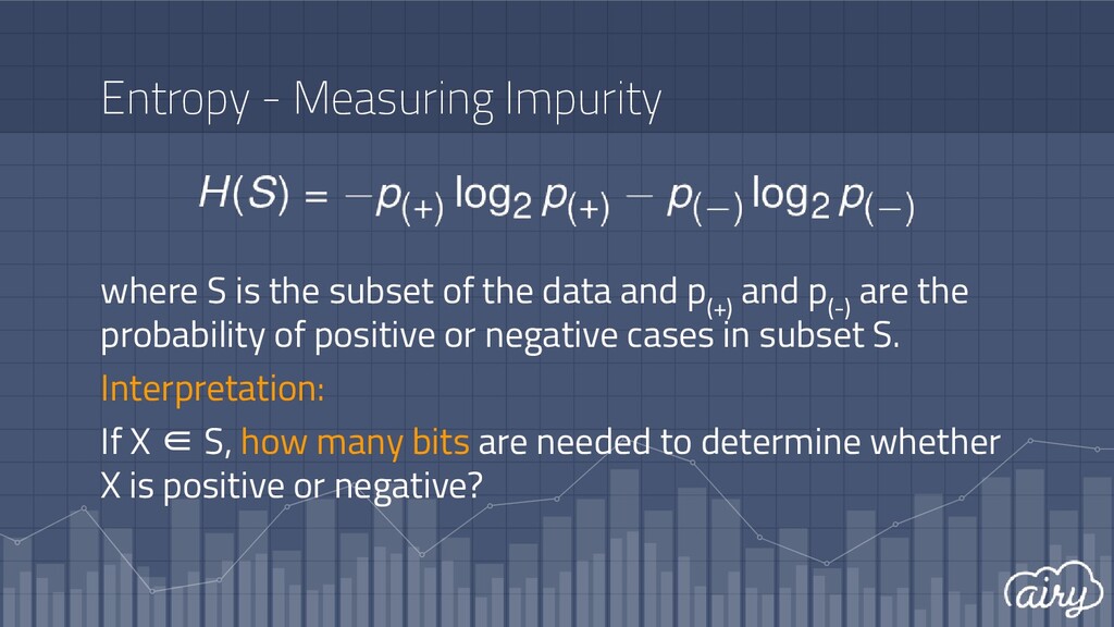
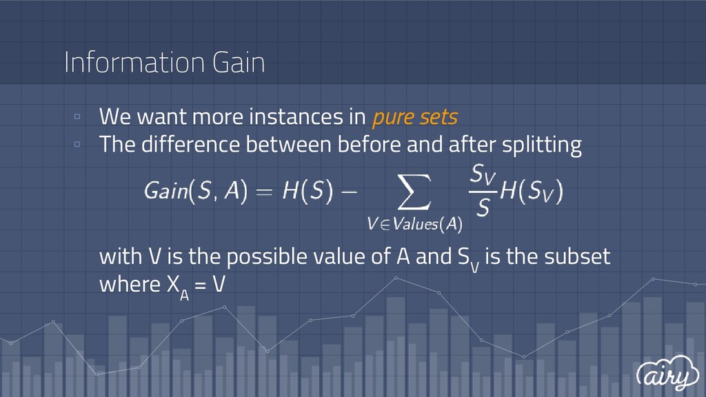
30. Entropy - Measuring Impurity where S is the subset of the data and p (+) and p (-) are the probability of positive or negative cases in subset S. Interpretation: If X ∈ S, how many bits are needed to determine whether X is positive or negative?
31. Information Gain ▫ We want more instances in pure sets ▫ The difference between before and after splitting with V is the possible value of A and S V is the subset where X A = V
32. Reducing features from 30 to 14 to predict the survival of Titanic passengers (Besbes, 2016)
33. Top 4% solution on Kaggle Titanic challenge
34. FEATURE EXTRACTION
35. Principal Component Analysis
36. References 1. VanderPlas, J. (2016). Python Data Science Handbook. (In Depth: Principal Component Analysis) 2. Leskovec, J., Rajaraman, A., & Ullman, J. D. (2014). Mining of massive datasets. Cambridge University Press. (Section 11.1-11.2)
37. Curse of Dimensionality ▫ High-dimensional datasets, e.g. images, text, speech ▫ Only a few “useful” dimensions ▫ Attributes with low variance
38. In MNIST, only a few pixels matter from R784
39. In social networks, not all people are connected
40. What else?
41. ▫ Speech → MFCC ▫ Text → bag of words, TF-IDF ▫ Image → Scale-Invariant Feature Transform (SIFT) Feature Extraction
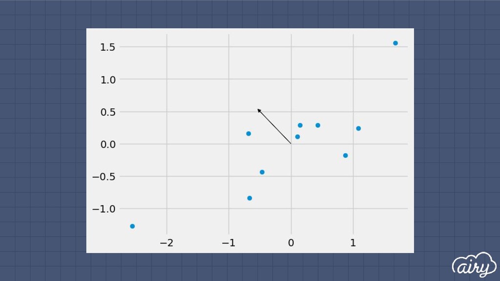
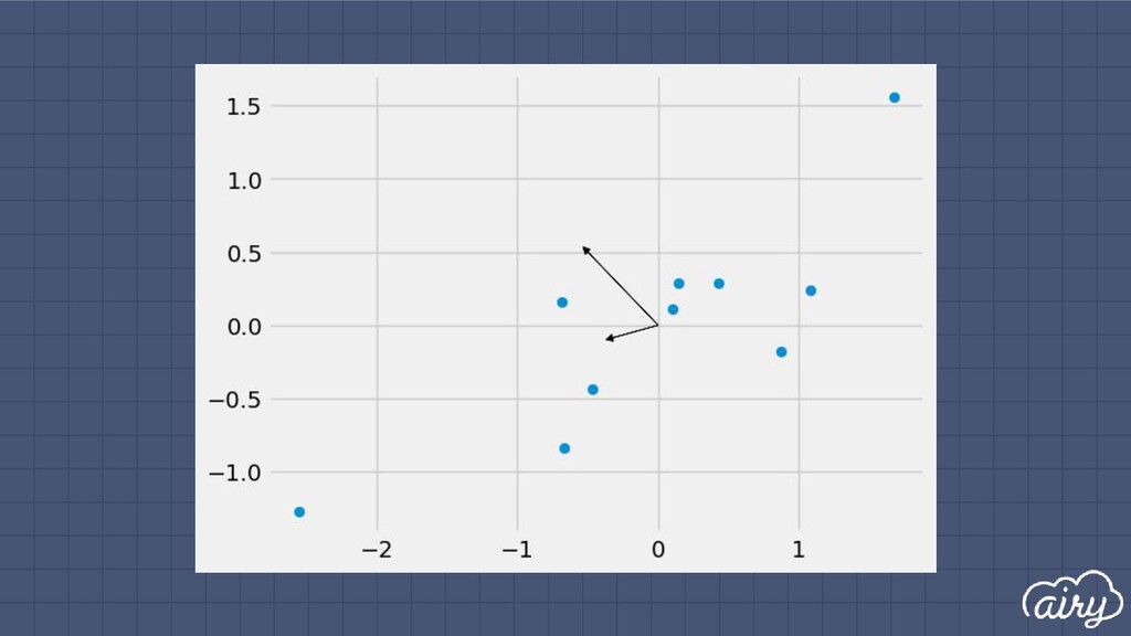
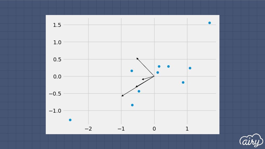
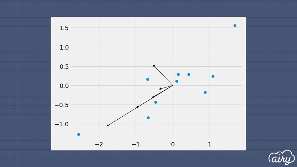
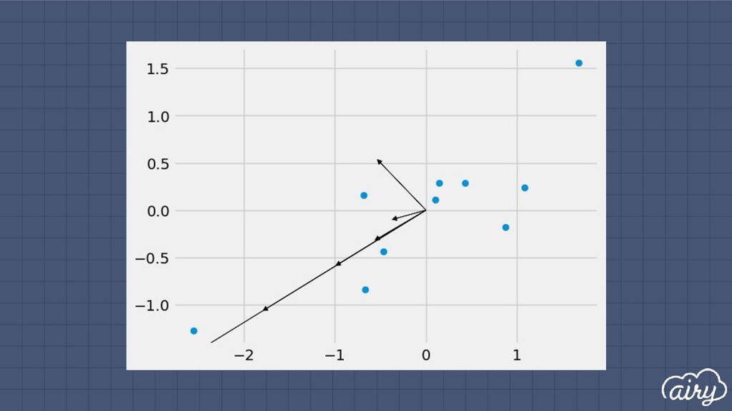
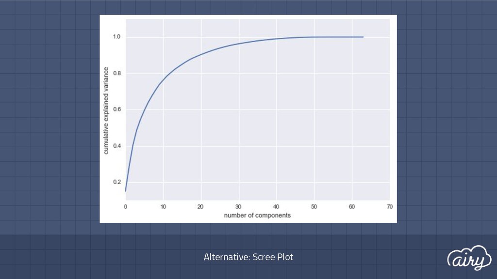
42. Principal Component Analysis 1. Defines a set of principal components a. 1st: direction of the greatest variability in the data b. 2nd: perpendicular to 1st, greatest variability of what’s left c. … and so on until d (original dimensionality) 2. First m << d components become m new dimensions
43. Example data in 2D (VanderPlas, 2016)
44. Two principal components (VanderPlas, 2016)
45. Data projection using principal components (VanderPlas, 2016)
46. PCA on Iris dataset
47. PCA on Iris dataset
48. 1. Center the data at zero: x i,a ← x i,a - µ 2. Compute covariance matrix Σ 3. Find eigenvectors e for that matrix Finding Principal Components
49. Let’s try to use the covariance matrix to transform a random vector! Finding Principal Components - Illustration
56. The vector’s direction is not changing after several iterations!
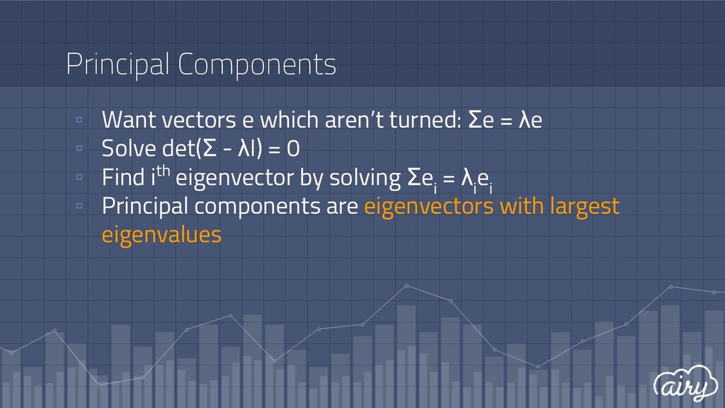
57. ▫ Want vectors e which aren’t turned: Σe = λe ▫ Solve det(Σ - λI) = 0 ▫ Find ith eigenvector by solving Σe i = λ i e i ▫ Principal components are eigenvectors with largest eigenvalues Principal Components
58. Example Given Σ = [2.0 0.8; 0.8 0.6], the eigenvalues are given by The eigenvalues are then
59. Example (cont.) The 1st eigenvector can then be calculated as follows
60. Projecting to New Dimensions ▫ e 1 ...e m are new dimension vectors ▫ For every data point x i : - Center to the mean, i.e. x i - µ - Project to the new dimensions, i.e. (x i -µ)Te j for j = 1...m
61. How many dimensions? Pick e i that “explains” the most variance ▫ Sort eigenvectors such that λ 1 ≥ λ 2 ≥ … ≥ λ d ▫ Pick first m eigenvectors which explain 90% or 95% of the total variance
62. Alternative: Scree Plot
63. PCA on customer vs property will cluster properties by their city!
64. When is it the most helpful?
65. ▫ Basically, PCA on text data ▫ Truncated Singular Value Decomposition (SVD) ▫ Capturing co-occurring words Latent Semantic Analysis (LSA)
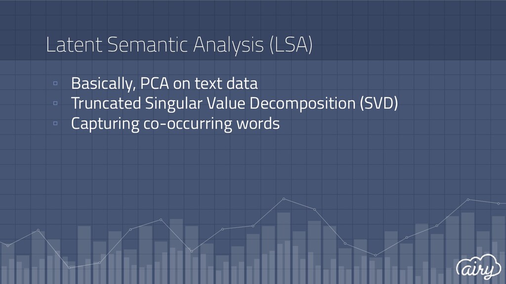
66. ▫ Automatic short-answer scoring ▫ Precision, recall, F1 scores on training set A (5-fold CV): - Without SVD (578 unique tokens): 84.52% | 92.15% | 88.06% - With SVD (100 features): 79.38% | 98.43% | 87.86% ▫ 3rd place on test set UKARA 1.0 Challenge Track 1
67. Faster training with PCA
68. Some Issues ▫ Sensitive to outliers when computing the covariance matrix → normalise the data ▫ Linearity assumption → transformation
69. Deep Learning
70. References ▫ Chollet, F. (May 2016). “Building Autoencoders in Keras”. The Keras Blog. ▫ Wibisono, O. (October 2017). “Autoencoder: Alternatif PCA yang Lebih Mumpuni”. Tentang Data.
71. Autoencoder: A neural network to map an input to itself (Chollet, 2016)
72. Learning curve of an autoencoder on MNIST (Wibisono, 2017)
73. Dimensionality reduction of MNIST using AE (above) and PCA (below) (Wibisono, 2017)
74. Pre-trained models for feature extraction (Wibisono, 2016)
75. Classifying amenities with ResNet50 and t-SNE
76. Thank you! Ali Akbar Septiandri Twitter: @__aliakbars__ Home: http:/ /uai.aliakbars.com Airy: https:/ /medium.com/airy-science