Upgrade to Pro — share decks privately, control downloads, hide ads and more …

Representing Higher-Order Networks: A Survey o...

Sponsored · Your Podcast. Everywhere. Effortlessly. Share. Educate. Inspire. Entertain. You do you. We'll handle the rest. →
Avatar for ASDG ASDG
April 08, 2026
0

Representing Higher-Order Networks: A Survey of Graph-Based Frameworks

Representing Higher-Order Networks:
A Survey of Graph-Based Frameworks

Avatar for ASDG

ASDG

April 08, 2026

Transcript

  1. Representing Higher-Order Networks: A Survey of Graph-Based Frameworks (Third Edition)

    Takaaki Fujita, Florentin Smarandache Neutrosophic Science International Association (NSIA) Publishing House Gallup - Guayaquil United States of America – Ecuador 2026
  2. Editor: Neutrosophic Science International Association (NSIA) Publishing House https://fs.unm.edu/NSIA/ Division

    of Mathematics and Sciences University of New Mexico 705 Gurley Ave., Gallup Campus NM 87301, United States of America University of Guayaquil Av. Kennedy and Av. Delta “Dr. Salvador Allende” University Campus Guayaquil 090514, Ecuador PEER REVIEWERS Mohamed Elhoseny American University in the Emirates, Dubai, UAE Email: [email protected] Young Bae Jun Gyeongsang National University, South Korea Email: [email protected] Yo-Ping Huang Department of Computer Science and Information, Engineering National Taipei University, New Taipei City, Taiwan Email: [email protected]
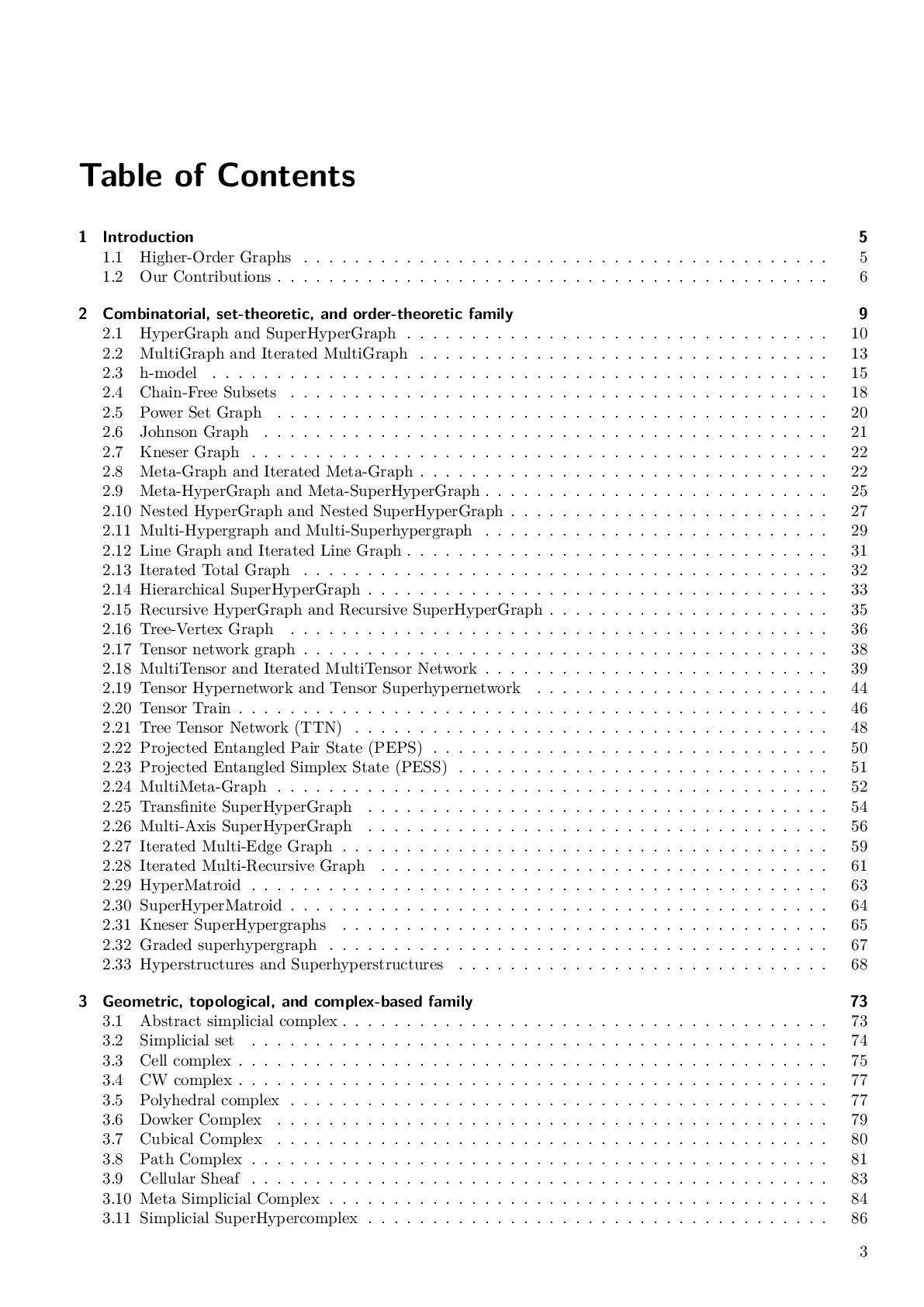
  3. Table of Contents 1 Introduction 5 1.1 Higher-Order Graphs .

    . . . . . . . . . . . . . . . . . . . . . . . . . . . . . . . . . . . . . . . . 5 1.2 Our Contributions . . . . . . . . . . . . . . . . . . . . . . . . . . . . . . . . . . . . . . . . . . . 6 2 Combinatorial, set-theoretic, and order-theoretic family 9 2.1 HyperGraph and SuperHyperGraph . . . . . . . . . . . . . . . . . . . . . . . . . . . . . . . . . 10 2.2 MultiGraph and Iterated MultiGraph . . . . . . . . . . . . . . . . . . . . . . . . . . . . . . . . 13 2.3 h-model . . . . . . . . . . . . . . . . . . . . . . . . . . . . . . . . . . . . . . . . . . . . . . . . 15 2.4 Chain-Free Subsets . . . . . . . . . . . . . . . . . . . . . . . . . . . . . . . . . . . . . . . . . . 18 2.5 Power Set Graph . . . . . . . . . . . . . . . . . . . . . . . . . . . . . . . . . . . . . . . . . . . 20 2.6 Johnson Graph . . . . . . . . . . . . . . . . . . . . . . . . . . . . . . . . . . . . . . . . . . . . 21 2.7 Kneser Graph . . . . . . . . . . . . . . . . . . . . . . . . . . . . . . . . . . . . . . . . . . . . . 22 2.8 Meta-Graph and Iterated Meta-Graph . . . . . . . . . . . . . . . . . . . . . . . . . . . . . . . . 22 2.9 Meta-HyperGraph and Meta-SuperHyperGraph . . . . . . . . . . . . . . . . . . . . . . . . . . . 25 2.10 Nested HyperGraph and Nested SuperHyperGraph . . . . . . . . . . . . . . . . . . . . . . . . . 27 2.11 Multi-Hypergraph and Multi-Superhypergraph . . . . . . . . . . . . . . . . . . . . . . . . . . . 29 2.12 Line Graph and Iterated Line Graph . . . . . . . . . . . . . . . . . . . . . . . . . . . . . . . . . 31 2.13 Iterated Total Graph . . . . . . . . . . . . . . . . . . . . . . . . . . . . . . . . . . . . . . . . . 32 2.14 Hierarchical SuperHyperGraph . . . . . . . . . . . . . . . . . . . . . . . . . . . . . . . . . . . . 33 2.15 Recursive HyperGraph and Recursive SuperHyperGraph . . . . . . . . . . . . . . . . . . . . . . 35 2.16 Tree-Vertex Graph . . . . . . . . . . . . . . . . . . . . . . . . . . . . . . . . . . . . . . . . . . 36 2.17 Tensor network graph . . . . . . . . . . . . . . . . . . . . . . . . . . . . . . . . . . . . . . . . . 38 2.18 MultiTensor and Iterated MultiTensor Network . . . . . . . . . . . . . . . . . . . . . . . . . . . 39 2.19 Tensor Hypernetwork and Tensor Superhypernetwork . . . . . . . . . . . . . . . . . . . . . . . 44 2.20 Tensor Train . . . . . . . . . . . . . . . . . . . . . . . . . . . . . . . . . . . . . . . . . . . . . . 46 2.21 Tree Tensor Network (TTN) . . . . . . . . . . . . . . . . . . . . . . . . . . . . . . . . . . . . . 48 2.22 Projected Entangled Pair State (PEPS) . . . . . . . . . . . . . . . . . . . . . . . . . . . . . . . 50 2.23 Projected Entangled Simplex State (PESS) . . . . . . . . . . . . . . . . . . . . . . . . . . . . . 51 2.24 MultiMeta-Graph . . . . . . . . . . . . . . . . . . . . . . . . . . . . . . . . . . . . . . . . . . . 52 2.25 Transfinite SuperHyperGraph . . . . . . . . . . . . . . . . . . . . . . . . . . . . . . . . . . . . 54 2.26 Multi-Axis SuperHyperGraph . . . . . . . . . . . . . . . . . . . . . . . . . . . . . . . . . . . . 56 2.27 Iterated Multi-Edge Graph . . . . . . . . . . . . . . . . . . . . . . . . . . . . . . . . . . . . . . 59 2.28 Iterated Multi-Recursive Graph . . . . . . . . . . . . . . . . . . . . . . . . . . . . . . . . . . . 61 2.29 HyperMatroid . . . . . . . . . . . . . . . . . . . . . . . . . . . . . . . . . . . . . . . . . . . . . 63 2.30 SuperHyperMatroid . . . . . . . . . . . . . . . . . . . . . . . . . . . . . . . . . . . . . . . . . . 64 2.31 Kneser SuperHypergraphs . . . . . . . . . . . . . . . . . . . . . . . . . . . . . . . . . . . . . . 65 2.32 Graded superhypergraph . . . . . . . . . . . . . . . . . . . . . . . . . . . . . . . . . . . . . . . 67 2.33 Hyperstructures and Superhyperstructures . . . . . . . . . . . . . . . . . . . . . . . . . . . . . 68 3 Geometric, topological, and complex-based family 73 3.1 Abstract simplicial complex . . . . . . . . . . . . . . . . . . . . . . . . . . . . . . . . . . . . . . 73 3.2 Simplicial set . . . . . . . . . . . . . . . . . . . . . . . . . . . . . . . . . . . . . . . . . . . . . 74 3.3 Cell complex . . . . . . . . . . . . . . . . . . . . . . . . . . . . . . . . . . . . . . . . . . . . . . 75 3.4 CW complex . . . . . . . . . . . . . . . . . . . . . . . . . . . . . . . . . . . . . . . . . . . . . . 77 3.5 Polyhedral complex . . . . . . . . . . . . . . . . . . . . . . . . . . . . . . . . . . . . . . . . . . 77 3.6 Dowker Complex . . . . . . . . . . . . . . . . . . . . . . . . . . . . . . . . . . . . . . . . . . . 79 3.7 Cubical Complex . . . . . . . . . . . . . . . . . . . . . . . . . . . . . . . . . . . . . . . . . . . 80 3.8 Path Complex . . . . . . . . . . . . . . . . . . . . . . . . . . . . . . . . . . . . . . . . . . . . . 81 3.9 Cellular Sheaf . . . . . . . . . . . . . . . . . . . . . . . . . . . . . . . . . . . . . . . . . . . . . 83 3.10 Meta Simplicial Complex . . . . . . . . . . . . . . . . . . . . . . . . . . . . . . . . . . . . . . . 84 3.11 Simplicial SuperHypercomplex . . . . . . . . . . . . . . . . . . . . . . . . . . . . . . . . . . . . 86 3
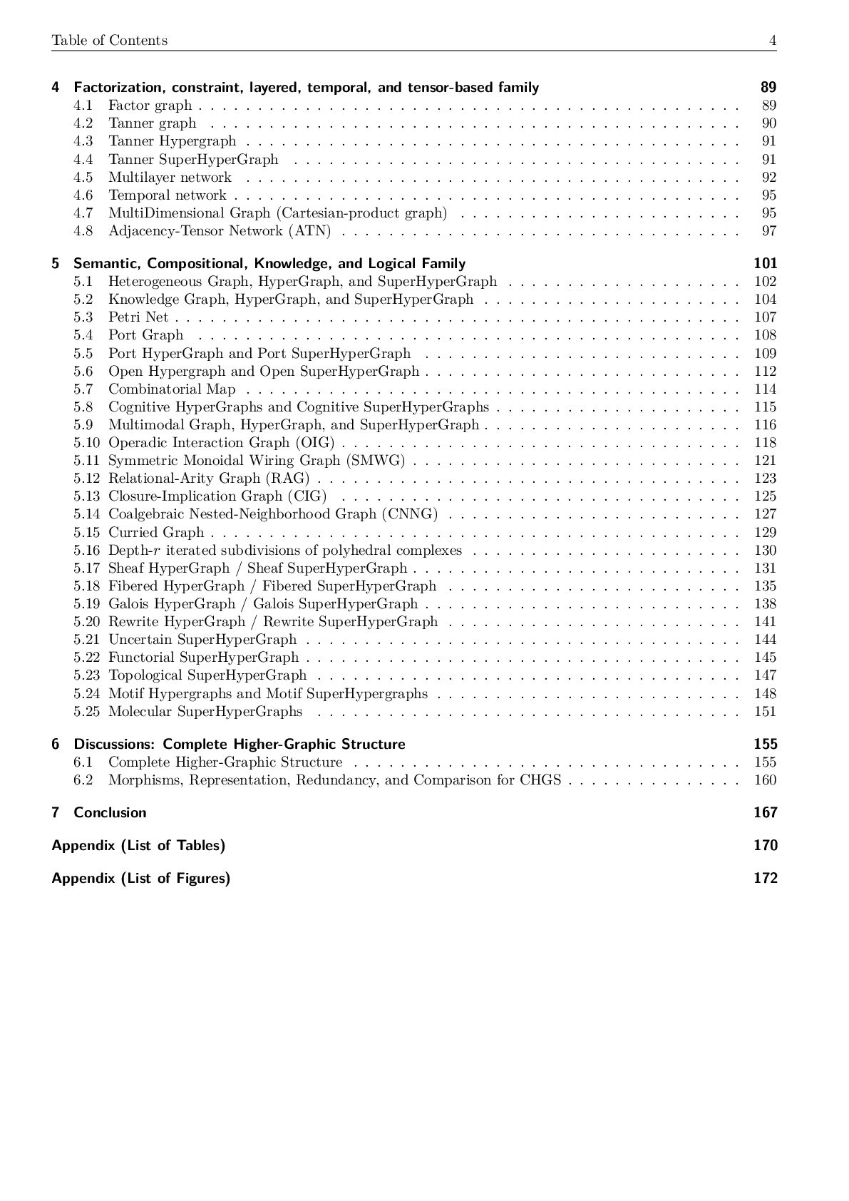
  4. Table of Contents 4 4 Factorization, constraint, layered, temporal, and

    tensor-based family 89 4.1 Factor graph . . . . . . . . . . . . . . . . . . . . . . . . . . . . . . . . . . . . . . . . . . . . . . 89 4.2 Tanner graph . . . . . . . . . . . . . . . . . . . . . . . . . . . . . . . . . . . . . . . . . . . . . 90 4.3 Tanner Hypergraph . . . . . . . . . . . . . . . . . . . . . . . . . . . . . . . . . . . . . . . . . . 91 4.4 Tanner SuperHyperGraph . . . . . . . . . . . . . . . . . . . . . . . . . . . . . . . . . . . . . . 91 4.5 Multilayer network . . . . . . . . . . . . . . . . . . . . . . . . . . . . . . . . . . . . . . . . . . 92 4.6 Temporal network . . . . . . . . . . . . . . . . . . . . . . . . . . . . . . . . . . . . . . . . . . . 95 4.7 MultiDimensional Graph (Cartesian-product graph) . . . . . . . . . . . . . . . . . . . . . . . . 95 4.8 Adjacency-Tensor Network (ATN) . . . . . . . . . . . . . . . . . . . . . . . . . . . . . . . . . . 97 5 Semantic, Compositional, Knowledge, and Logical Family 101 5.1 Heterogeneous Graph, HyperGraph, and SuperHyperGraph . . . . . . . . . . . . . . . . . . . . 102 5.2 Knowledge Graph, HyperGraph, and SuperHyperGraph . . . . . . . . . . . . . . . . . . . . . . 104 5.3 Petri Net . . . . . . . . . . . . . . . . . . . . . . . . . . . . . . . . . . . . . . . . . . . . . . . . 107 5.4 Port Graph . . . . . . . . . . . . . . . . . . . . . . . . . . . . . . . . . . . . . . . . . . . . . . 108 5.5 Port HyperGraph and Port SuperHyperGraph . . . . . . . . . . . . . . . . . . . . . . . . . . . 109 5.6 Open Hypergraph and Open SuperHyperGraph . . . . . . . . . . . . . . . . . . . . . . . . . . . 112 5.7 Combinatorial Map . . . . . . . . . . . . . . . . . . . . . . . . . . . . . . . . . . . . . . . . . . 114 5.8 Cognitive HyperGraphs and Cognitive SuperHyperGraphs . . . . . . . . . . . . . . . . . . . . . 115 5.9 Multimodal Graph, HyperGraph, and SuperHyperGraph . . . . . . . . . . . . . . . . . . . . . . 116 5.10 Operadic Interaction Graph (OIG) . . . . . . . . . . . . . . . . . . . . . . . . . . . . . . . . . . 118 5.11 Symmetric Monoidal Wiring Graph (SMWG) . . . . . . . . . . . . . . . . . . . . . . . . . . . . 121 5.12 Relational-Arity Graph (RAG) . . . . . . . . . . . . . . . . . . . . . . . . . . . . . . . . . . . . 123 5.13 Closure-Implication Graph (CIG) . . . . . . . . . . . . . . . . . . . . . . . . . . . . . . . . . . 125 5.14 Coalgebraic Nested-Neighborhood Graph (CNNG) . . . . . . . . . . . . . . . . . . . . . . . . . 127 5.15 Curried Graph . . . . . . . . . . . . . . . . . . . . . . . . . . . . . . . . . . . . . . . . . . . . . 129 5.16 Depth-r iterated subdivisions of polyhedral complexes . . . . . . . . . . . . . . . . . . . . . . . 130 5.17 Sheaf HyperGraph / Sheaf SuperHyperGraph . . . . . . . . . . . . . . . . . . . . . . . . . . . . 131 5.18 Fibered HyperGraph / Fibered SuperHyperGraph . . . . . . . . . . . . . . . . . . . . . . . . . 135 5.19 Galois HyperGraph / Galois SuperHyperGraph . . . . . . . . . . . . . . . . . . . . . . . . . . . 138 5.20 Rewrite HyperGraph / Rewrite SuperHyperGraph . . . . . . . . . . . . . . . . . . . . . . . . . 141 5.21 Uncertain SuperHyperGraph . . . . . . . . . . . . . . . . . . . . . . . . . . . . . . . . . . . . . 144 5.22 Functorial SuperHyperGraph . . . . . . . . . . . . . . . . . . . . . . . . . . . . . . . . . . . . . 145 5.23 Topological SuperHyperGraph . . . . . . . . . . . . . . . . . . . . . . . . . . . . . . . . . . . . 147 5.24 Motif Hypergraphs and Motif SuperHypergraphs . . . . . . . . . . . . . . . . . . . . . . . . . . 148 5.25 Molecular SuperHyperGraphs . . . . . . . . . . . . . . . . . . . . . . . . . . . . . . . . . . . . 151 6 Discussions: Complete Higher-Graphic Structure 155 6.1 Complete Higher-Graphic Structure . . . . . . . . . . . . . . . . . . . . . . . . . . . . . . . . . 155 6.2 Morphisms, Representation, Redundancy, and Comparison for CHGS . . . . . . . . . . . . . . . 160 7 Conclusion 167 Appendix (List of Tables) 170 Appendix (List of Figures) 172
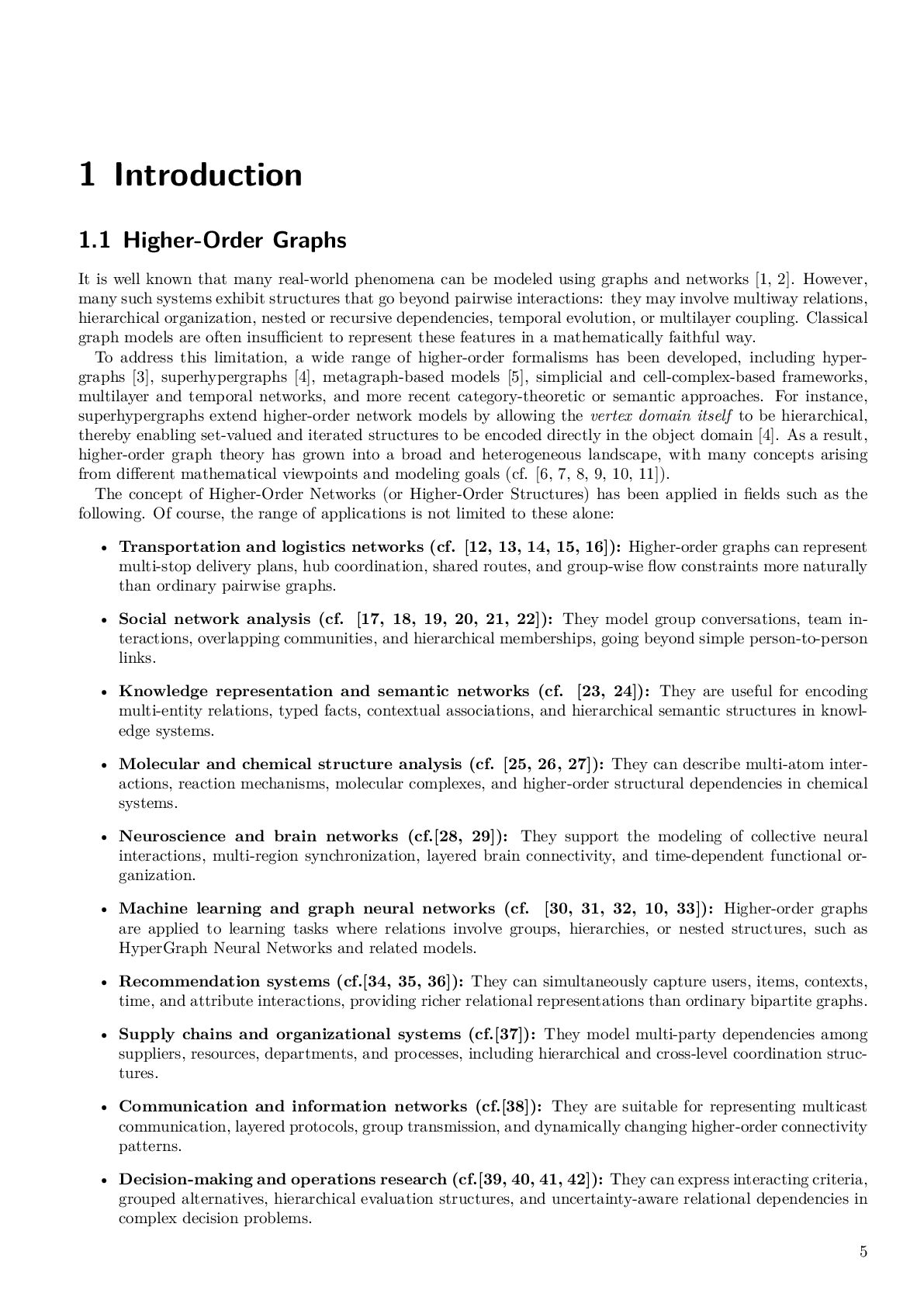
  5. 1 Introduction 1.1 Higher-Order Graphs It is well known that

    many real-world phenomena can be modeled using graphs and networks [1, 2]. However, many such systems exhibit structures that go beyond pairwise interactions: they may involve multiway relations, hierarchical organization, nested or recursive dependencies, temporal evolution, or multilayer coupling. Classical graph models are often insufficient to represent these features in a mathematically faithful way. To address this limitation, a wide range of higher-order formalisms has been developed, including hyper- graphs [3], superhypergraphs [4], metagraph-based models [5], simplicial and cell-complex-based frameworks, multilayer and temporal networks, and more recent category-theoretic or semantic approaches. For instance, superhypergraphs extend higher-order network models by allowing the vertex domain itself to be hierarchical, thereby enabling set-valued and iterated structures to be encoded directly in the object domain [4]. As a result, higher-order graph theory has grown into a broad and heterogeneous landscape, with many concepts arising from different mathematical viewpoints and modeling goals (cf. [6, 7, 8, 9, 10, 11]). The concept of Higher-Order Networks (or Higher-Order Structures) has been applied in fields such as the following. Of course, the range of applications is not limited to these alone: • Transportation and logistics networks (cf. [12, 13, 14, 15, 16]): Higher-order graphs can represent multi-stop delivery plans, hub coordination, shared routes, and group-wise flow constraints more naturally than ordinary pairwise graphs. • Social network analysis (cf. [17, 18, 19, 20, 21, 22]): They model group conversations, team in- teractions, overlapping communities, and hierarchical memberships, going beyond simple person-to-person links. • Knowledge representation and semantic networks (cf. [23, 24]): They are useful for encoding multi-entity relations, typed facts, contextual associations, and hierarchical semantic structures in knowl- edge systems. • Molecular and chemical structure analysis (cf. [25, 26, 27]): They can describe multi-atom inter- actions, reaction mechanisms, molecular complexes, and higher-order structural dependencies in chemical systems. • Neuroscience and brain networks (cf.[28, 29]): They support the modeling of collective neural interactions, multi-region synchronization, layered brain connectivity, and time-dependent functional or- ganization. • Machine learning and graph neural networks (cf. [30, 31, 32, 10, 33]): Higher-order graphs are applied to learning tasks where relations involve groups, hierarchies, or nested structures, such as HyperGraph Neural Networks and related models. • Recommendation systems (cf.[34, 35, 36]): They can simultaneously capture users, items, contexts, time, and attribute interactions, providing richer relational representations than ordinary bipartite graphs. • Supply chains and organizational systems (cf.[37]): They model multi-party dependencies among suppliers, resources, departments, and processes, including hierarchical and cross-level coordination struc- tures. • Communication and information networks (cf.[38]): They are suitable for representing multicast communication, layered protocols, group transmission, and dynamically changing higher-order connectivity patterns. • Decision-making and operations research (cf.[39, 40, 41, 42]): They can express interacting criteria, grouped alternatives, hierarchical evaluation structures, and uncertainty-aware relational dependencies in complex decision problems. 5
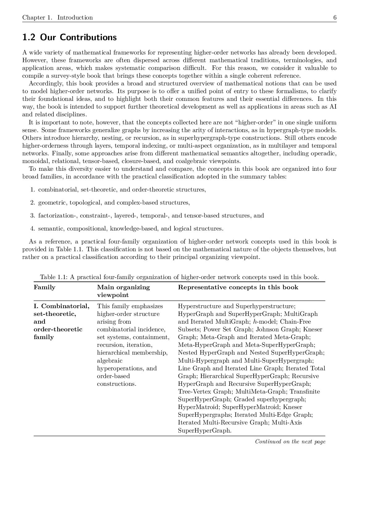
  6. Chapter 1. Introduction 6 1.2 Our Contributions A wide variety

    of mathematical frameworks for representing higher-order networks has already been developed. However, these frameworks are often dispersed across different mathematical traditions, terminologies, and application areas, which makes systematic comparison difficult. For this reason, we consider it valuable to compile a survey-style book that brings these concepts together within a single coherent reference. Accordingly, this book provides a broad and structured overview of mathematical notions that can be used to model higher-order networks. Its purpose is to offer a unified point of entry to these formalisms, to clarify their foundational ideas, and to highlight both their common features and their essential differences. In this way, the book is intended to support further theoretical development as well as applications in areas such as AI and related disciplines. It is important to note, however, that the concepts collected here are not “higher-order” in one single uniform sense. Some frameworks generalize graphs by increasing the arity of interactions, as in hypergraph-type models. Others introduce hierarchy, nesting, or recursion, as in superhypergraph-type constructions. Still others encode higher-orderness through layers, temporal indexing, or multi-aspect organization, as in multilayer and temporal networks. Finally, some approaches arise from different mathematical semantics altogether, including operadic, monoidal, relational, tensor-based, closure-based, and coalgebraic viewpoints. To make this diversity easier to understand and compare, the concepts in this book are organized into four broad families, in accordance with the practical classification adopted in the summary tables: 1. combinatorial, set-theoretic, and order-theoretic structures, 2. geometric, topological, and complex-based structures, 3. factorization-, constraint-, layered-, temporal-, and tensor-based structures, and 4. semantic, compositional, knowledge-based, and logical structures. As a reference, a practical four-family organization of higher-order network concepts used in this book is provided in Table 1.1. This classification is not based on the mathematical nature of the objects themselves, but rather on a practical classification according to their principal organizing viewpoint. Table 1.1: A practical four-family organization of higher-order network concepts used in this book. Family Main organizing viewpoint Representative concepts in this book I. Combinatorial, set-theoretic, and order-theoretic family This family emphasizes higher-order structure arising from combinatorial incidence, set systems, containment, recursion, iteration, hierarchical membership, algebraic hyperoperations, and order-based constructions. Hyperstructure and Superhyperstructure; HyperGraph and SuperHyperGraph; MultiGraph and Iterated MultiGraph; h-model; Chain-Free Subsets; Power Set Graph; Johnson Graph; Kneser Graph; Meta-Graph and Iterated Meta-Graph; Meta-HyperGraph and Meta-SuperHyperGraph; Nested HyperGraph and Nested SuperHyperGraph; Multi-Hypergraph and Multi-SuperHypergraph; Line Graph and Iterated Line Graph; Iterated Total Graph; Hierarchical SuperHyperGraph; Recursive HyperGraph and Recursive SuperHyperGraph; Tree-Vertex Graph; MultiMeta-Graph; Transfinite SuperHyperGraph; Graded superhypergraph; HyperMatroid; SuperHyperMatroid; Kneser SuperHypergraphs; Iterated Multi-Edge Graph; Iterated Multi-Recursive Graph; Multi-Axis SuperHyperGraph. Continued on the next page
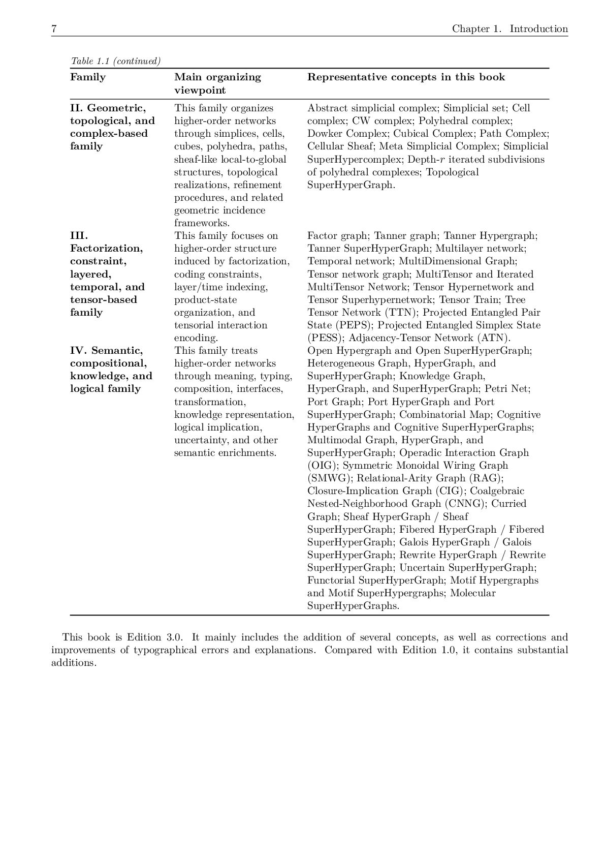
  7. 7 Chapter 1. Introduction Table 1.1 (continued) Family Main organizing

    viewpoint Representative concepts in this book II. Geometric, topological, and complex-based family This family organizes higher-order networks through simplices, cells, cubes, polyhedra, paths, sheaf-like local-to-global structures, topological realizations, refinement procedures, and related geometric incidence frameworks. Abstract simplicial complex; Simplicial set; Cell complex; CW complex; Polyhedral complex; Dowker Complex; Cubical Complex; Path Complex; Cellular Sheaf; Meta Simplicial Complex; Simplicial SuperHypercomplex; Depth-r iterated subdivisions of polyhedral complexes; Topological SuperHyperGraph. III. Factorization, constraint, layered, temporal, and tensor-based family This family focuses on higher-order structure induced by factorization, coding constraints, layer/time indexing, product-state organization, and tensorial interaction encoding. Factor graph; Tanner graph; Tanner Hypergraph; Tanner SuperHyperGraph; Multilayer network; Temporal network; MultiDimensional Graph; Tensor network graph; MultiTensor and Iterated MultiTensor Network; Tensor Hypernetwork and Tensor Superhypernetwork; Tensor Train; Tree Tensor Network (TTN); Projected Entangled Pair State (PEPS); Projected Entangled Simplex State (PESS); Adjacency-Tensor Network (ATN). IV. Semantic, compositional, knowledge, and logical family This family treats higher-order networks through meaning, typing, composition, interfaces, transformation, knowledge representation, logical implication, uncertainty, and other semantic enrichments. Open Hypergraph and Open SuperHyperGraph; Heterogeneous Graph, HyperGraph, and SuperHyperGraph; Knowledge Graph, HyperGraph, and SuperHyperGraph; Petri Net; Port Graph; Port HyperGraph and Port SuperHyperGraph; Combinatorial Map; Cognitive HyperGraphs and Cognitive SuperHyperGraphs; Multimodal Graph, HyperGraph, and SuperHyperGraph; Operadic Interaction Graph (OIG); Symmetric Monoidal Wiring Graph (SMWG); Relational-Arity Graph (RAG); Closure-Implication Graph (CIG); Coalgebraic Nested-Neighborhood Graph (CNNG); Curried Graph; Sheaf HyperGraph / Sheaf SuperHyperGraph; Fibered HyperGraph / Fibered SuperHyperGraph; Galois HyperGraph / Galois SuperHyperGraph; Rewrite HyperGraph / Rewrite SuperHyperGraph; Uncertain SuperHyperGraph; Functorial SuperHyperGraph; Motif Hypergraphs and Motif SuperHypergraphs; Molecular SuperHyperGraphs. This book is Edition 3.0. It mainly includes the addition of several concepts, as well as corrections and improvements of typographical errors and explanations. Compared with Edition 1.0, it contains substantial additions.
  8. Representing Higher-Order Networks: A Survey of Graph-Based Frameworks (Third Edition)

    Takaaki Fujita 1 ∗ and Florentin Smarandache2 1 Independent Researcher, Tokyo, Japan. 2 Email: [email protected] University of New Mexico, Gallup Campus, NM 87301, USA. Email: [email protected] Abstract Many real-world phenomena are naturally modeled by graphs and networks. However, classical graph models are often limited to pairwise interactions and may not adequately capture the richer structures that arise in practice. Higher-order graph formalisms extend this framework by incorporating multiway, hierarchical, tem- poral, multilayer, recursive, and tensor-based interactions, thereby providing more expressive representations of complex systems. This book presents a comprehensive overview of mathematical notions that can be used to model higher-order networks. It surveys foundational concepts, extensional frameworks, and newly introduced formalisms, with an emphasis on their structural principles, relationships, and modeling roles. The aim is to provide a unified perspective that helps readers compare diverse higher-order network models and identify appropriate tools for theoretical study and practical applications. This book is Edition 3.0. It mainly includes the addition of several concepts, as well as corrections and improvements of typographical errors and explanations. Compared with Edition 1.0, it contains substantial additions. Keywords: Hypergraph, Superhypergraph, Higher-Order Graphs MSC2010 (Mathematics Subject Classification 2010): 05C65 - Hypergraphs, 05C82 - Graph theory with applications
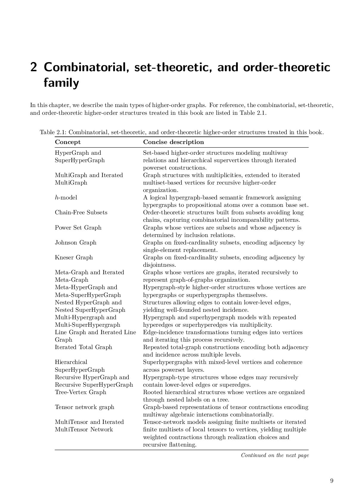
  9. 2 Combinatorial, set-theoretic, and order-theoretic family In this chapter, we

    describe the main types of higher-order graphs. For reference, the combinatorial, set-theoretic, and order-theoretic higher-order structures treated in this book are listed in Table 2.1. Table 2.1: Combinatorial, set-theoretic, and order-theoretic higher-order structures treated in this book. Concept Concise description HyperGraph and SuperHyperGraph Set-based higher-order structures modeling multiway relations and hierarchical supervertices through iterated powerset constructions. MultiGraph and Iterated MultiGraph Graph structures with multiplicities, extended to iterated multiset-based vertices for recursive higher-order organization. h-model A logical hypergraph-based semantic framework assigning hypergraphs to propositional atoms over a common base set. Chain-Free Subsets Order-theoretic structures built from subsets avoiding long chains, capturing combinatorial incomparability patterns. Power Set Graph Graphs whose vertices are subsets and whose adjacency is determined by inclusion relations. Johnson Graph Graphs on fixed-cardinality subsets, encoding adjacency by single-element replacement. Kneser Graph Graphs on fixed-cardinality subsets, encoding adjacency by disjointness. Meta-Graph and Iterated Meta-Graph Graphs whose vertices are graphs, iterated recursively to represent graph-of-graphs organization. Meta-HyperGraph and Meta-SuperHyperGraph Hypergraph-style higher-order structures whose vertices are hypergraphs or superhypergraphs themselves. Nested HyperGraph and Nested SuperHyperGraph Structures allowing edges to contain lower-level edges, yielding well-founded nested incidence. Multi-Hypergraph and Multi-SuperHypergraph Hypergraph and superhypergraph models with repeated hyperedges or superhyperedges via multiplicity. Line Graph and Iterated Line Graph Edge-incidence transformations turning edges into vertices and iterating this process recursively. Iterated Total Graph Repeated total-graph constructions encoding both adjacency and incidence across multiple levels. Hierarchical SuperHyperGraph Superhypergraphs with mixed-level vertices and coherence across powerset layers. Recursive HyperGraph and Recursive SuperHyperGraph Hypergraph-type structures whose edges may recursively contain lower-level edges or superedges. Tree-Vertex Graph Rooted hierarchical structures whose vertices are organized through nested labels on a tree. Tensor network graph Graph-based representations of tensor contractions encoding multiway algebraic interactions combinatorially. MultiTensor and Iterated MultiTensor Network Tensor-network models assigning finite multisets or iterated finite multisets of local tensors to vertices, yielding multiple weighted contractions through realization choices and recursive flattening. Continued on the next page 9
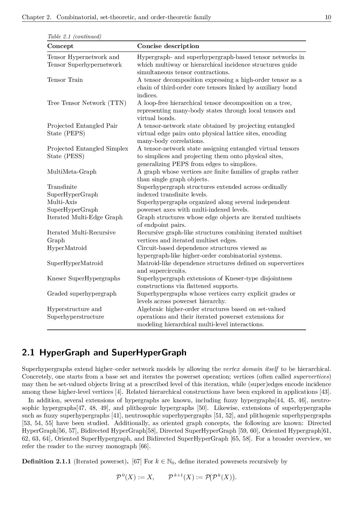
  10. Chapter 2. Combinatorial, set-theoretic, and order-theoretic family 10 Table 2.1

    (continued) Concept Concise description Tensor Hypernetwork and Tensor Superhypernetwork Hypergraph- and superhypergraph-based tensor networks in which multiway or hierarchical incidence structures guide simultaneous tensor contractions. Tensor Train A tensor decomposition expressing a high-order tensor as a chain of third-order core tensors linked by auxiliary bond indices. Tree Tensor Network (TTN) A loop-free hierarchical tensor decomposition on a tree, representing many-body states through local tensors and virtual bonds. Projected Entangled Pair State (PEPS) A tensor-network state obtained by projecting entangled virtual edge pairs onto physical lattice sites, encoding many-body correlations. Projected Entangled Simplex State (PESS) A tensor-network state assigning entangled virtual tensors to simplices and projecting them onto physical sites, generalizing PEPS from edges to simplices. MultiMeta-Graph A graph whose vertices are finite families of graphs rather than single graph objects. Transfinite SuperHyperGraph Superhypergraph structures extended across ordinally indexed transfinite levels. Multi-Axis SuperHyperGraph Superhypergraphs organized along several independent powerset axes with multi-indexed levels. Iterated Multi-Edge Graph Graph structures whose edge objects are iterated multisets of endpoint pairs. Iterated Multi-Recursive Graph Recursive graph-like structures combining iterated multiset vertices and iterated multiset edges. HyperMatroid Circuit-based dependence structures viewed as hypergraph-like higher-order combinatorial systems. SuperHyperMatroid Matroid-like dependence structures defined on supervertices and supercircuits. Kneser SuperHypergraphs Superhypergraph extensions of Kneser-type disjointness constructions via flattened supports. Graded superhypergraph Superhypergraphs whose vertices carry explicit grades or levels across powerset hierarchy. Hyperstructure and Superhyperstructure Algebraic higher-order structures based on set-valued operations and their iterated powerset extensions for modeling hierarchical multi-level interactions. 2.1 HyperGraph and SuperHyperGraph Superhypergraphs extend higher–order network models by allowing the vertex domain itself to be hierarchical. Concretely, one starts from a base set and iterates the powerset operation; vertices (often called supervertices) may then be set-valued objects living at a prescribed level of this iteration, while (super)edges encode incidence among these higher-level vertices [4]. Related hierarchical constructions have been explored in applications [43]. In addition, several extensions of hypergraphs are known, including fuzzy hypergraphs[44, 45, 46], neutro- sophic hypergraphs[47, 48, 49], and plithogenic hypergraphs [50]. Likewise, extensions of superhypergraphs such as fuzzy superhypergraphs [41], neutrosophic superhypergraphs [51, 52], and plithogenic superhypergraphs [53, 54, 55] have been studied. Additionally, as oriented graph concepts, the following are known: Directed HyperGraph[56, 57], Bidirected HyperGraph[58], Directed SuperHyperGraph [59, 60], Oriented Hypergraph[61, 62, 63, 64], Oriented SuperHypergraph, and Bidirected SuperHyperGraph [65, 58]. For a broader overview, we refer the reader to the survey monograph [66]. Definition 2.1.1 (Iterated powerset). [67] For k ∈ N0 , define iterated powersets recursively by P 0(X) := X, P k+1(X) := P P k(X) .
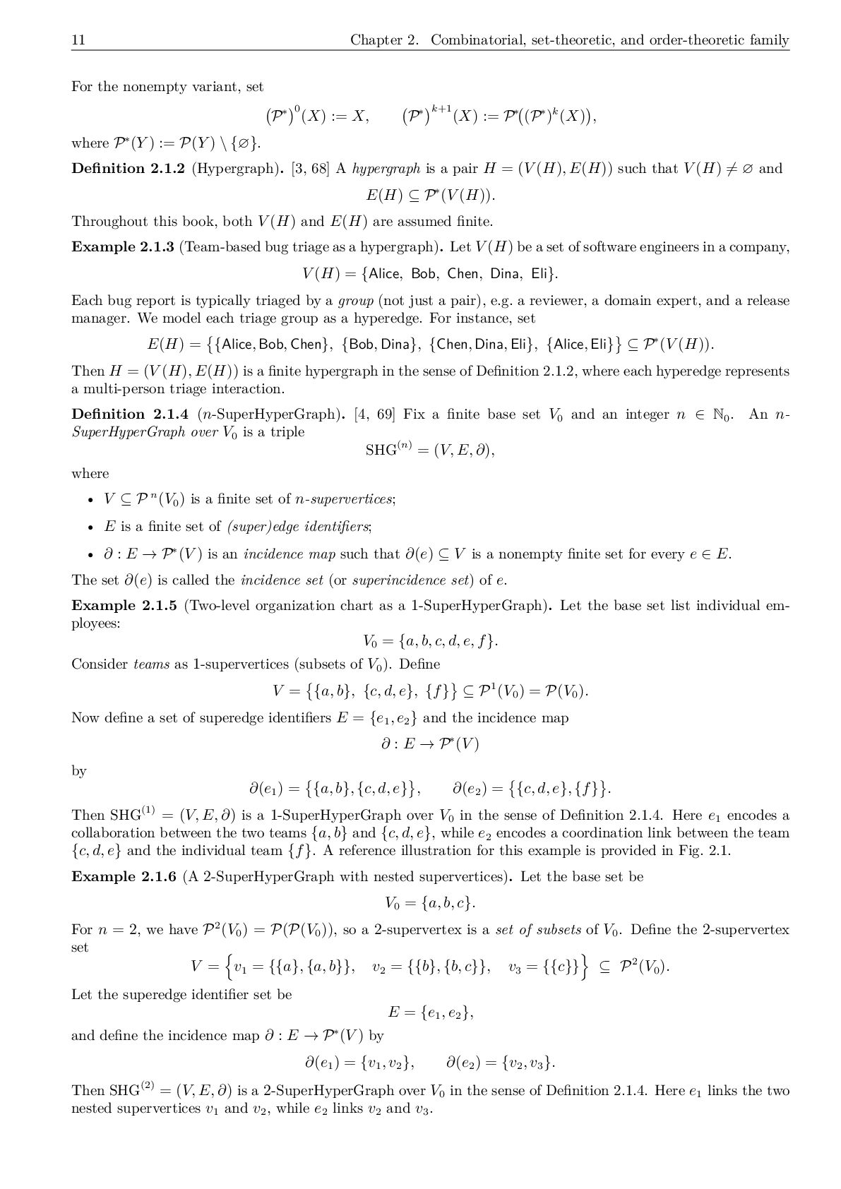
  11. 11 Chapter 2. Combinatorial, set-theoretic, and order-theoretic family For the

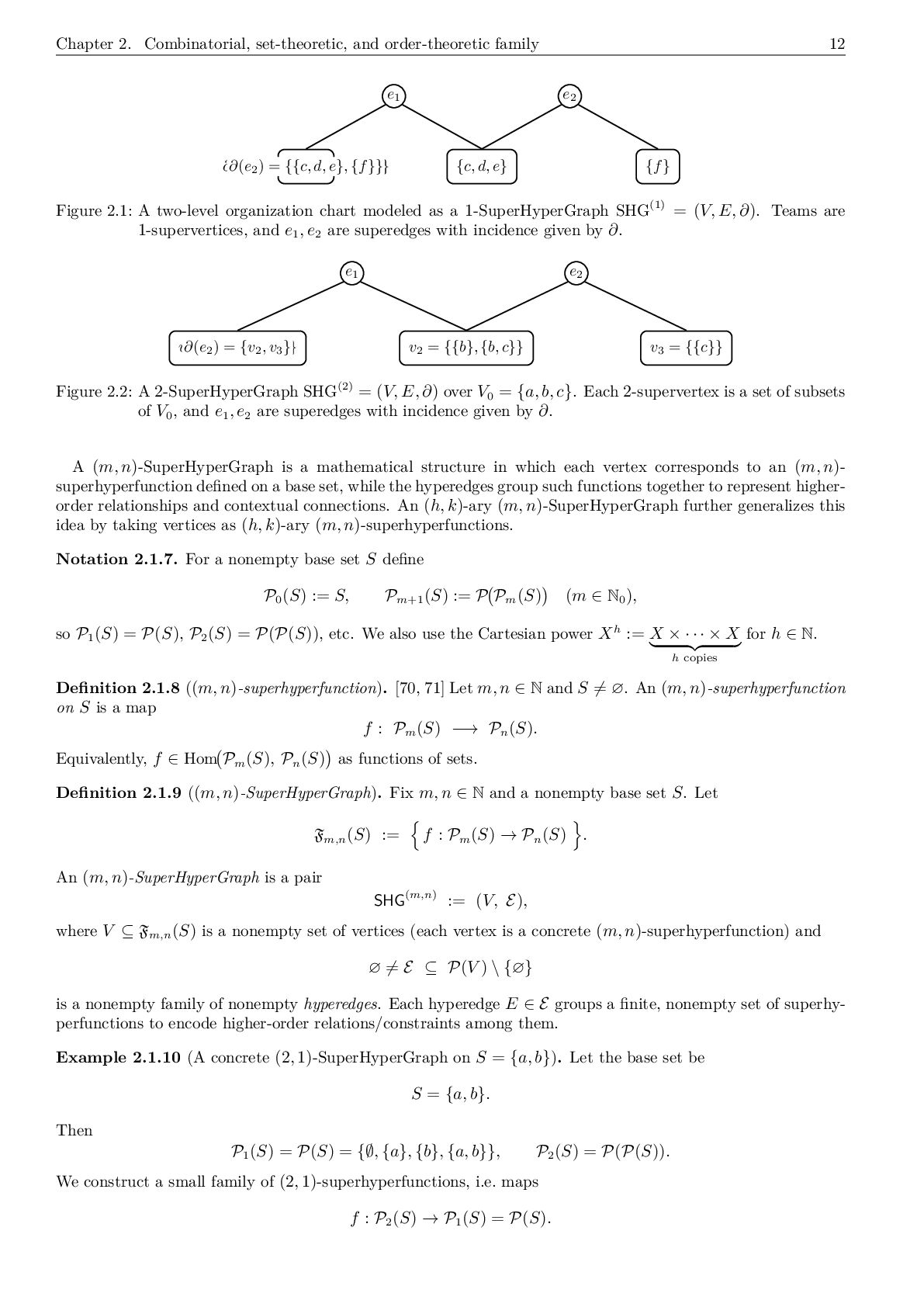
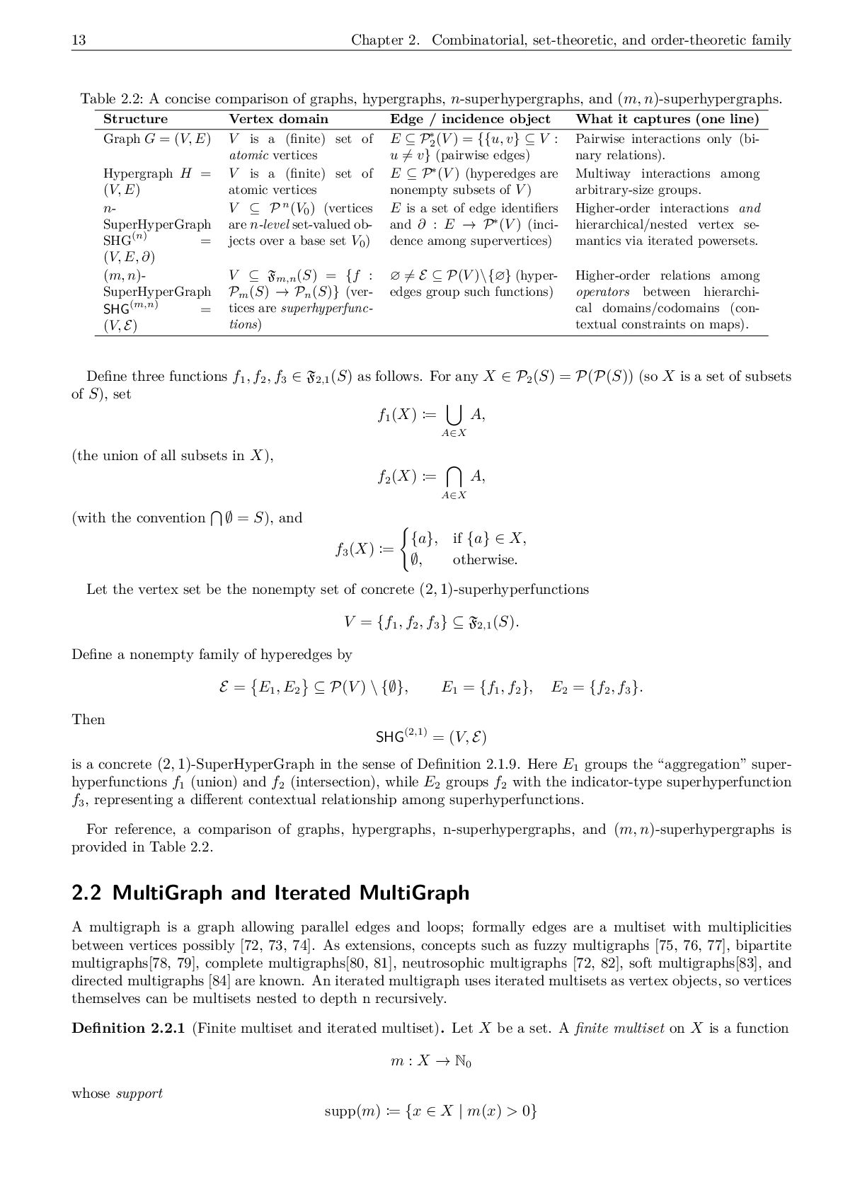
    nonempty variant, set P∗ 0 (X) := X, P∗ k+1 (X) := P∗ (P∗)k(X) , where P∗(Y ) := P(Y ) \ {∅}. Definition 2.1.2 (Hypergraph). [3, 68] A hypergraph is a pair H = (V (H), E(H)) such that V (H) = ∅ and E(H) ⊆ P∗(V (H)). Throughout this book, both V (H) and E(H) are assumed finite. Example 2.1.3 (Team-based bug triage as a hypergraph). Let V (H) be a set of software engineers in a company, V (H) = {Alice, Bob, Chen, Dina, Eli}. Each bug report is typically triaged by a group (not just a pair), e.g. a reviewer, a domain expert, and a release manager. We model each triage group as a hyperedge. For instance, set E(H) = {Alice, Bob, Chen}, {Bob, Dina}, {Chen, Dina, Eli}, {Alice, Eli} ⊆ P∗(V (H)). Then H = (V (H), E(H)) is a finite hypergraph in the sense of Definition 2.1.2, where each hyperedge represents a multi-person triage interaction. Definition 2.1.4 (n-SuperHyperGraph). [4, 69] Fix a finite base set V0 and an integer n ∈ N0 . An n- SuperHyperGraph over V0 is a triple SHG(n) = (V, E, ∂), where • V ⊆ P n(V0 ) is a finite set of n-supervertices; • E is a finite set of (super)edge identifiers; • ∂ : E → P∗(V ) is an incidence map such that ∂(e) ⊆ V is a nonempty finite set for every e ∈ E. The set ∂(e) is called the incidence set (or superincidence set) of e. Example 2.1.5 (Two-level organization chart as a 1-SuperHyperGraph). Let the base set list individual em- ployees: V0 = {a, b, c, d, e, f}. Consider teams as 1-supervertices (subsets of V0 ). Define V = {a, b}, {c, d, e}, {f} ⊆ P1(V0 ) = P(V0 ). Now define a set of superedge identifiers E = {e1 , e2 } and the incidence map ∂ : E → P∗(V ) by ∂(e1 ) = {a, b}, {c, d, e} , ∂(e2 ) = {c, d, e}, {f} . Then SHG(1) = (V, E, ∂) is a 1-SuperHyperGraph over V0 in the sense of Definition 2.1.4. Here e1 encodes a collaboration between the two teams {a, b} and {c, d, e}, while e2 encodes a coordination link between the team {c, d, e} and the individual team {f}. A reference illustration for this example is provided in Fig. 2.1. Example 2.1.6 (A 2-SuperHyperGraph with nested supervertices). Let the base set be V0 = {a, b, c}. For n = 2, we have P2(V0 ) = P(P(V0 )), so a 2-supervertex is a set of subsets of V0 . Define the 2-supervertex set V = v1 = {{a}, {a, b}}, v2 = {{b}, {b, c}}, v3 = {{c}} ⊆ P2(V0 ). Let the superedge identifier set be E = {e1 , e2 }, and define the incidence map ∂ : E → P∗(V ) by ∂(e1 ) = {v1 , v2 }, ∂(e2 ) = {v2 , v3 }. Then SHG(2) = (V, E, ∂) is a 2-SuperHyperGraph over V0 in the sense of Definition 2.1.4. Here e1 links the two nested supervertices v1 and v2 , while e2 links v2 and v3 .
  12. Chapter 2. Combinatorial, set-theoretic, and order-theoretic family 12 {a, b}

    {c, d, e} {f} e1 e2 ∂(e1 ) = {{a, b}, {c, d, e}} ∂(e2 ) = {{c, d, e}, {f}} Figure 2.1: A two-level organization chart modeled as a 1-SuperHyperGraph SHG(1) = (V, E, ∂). Teams are 1-supervertices, and e1 , e2 are superedges with incidence given by ∂. v1 = {{a}, {a, b}} v2 = {{b}, {b, c}} v3 = {{c}} e1 e2 ∂(e1 ) = {v1 , v2 } ∂(e2 ) = {v2 , v3 } Figure 2.2: A 2-SuperHyperGraph SHG(2) = (V, E, ∂) over V0 = {a, b, c}. Each 2-supervertex is a set of subsets of V0 , and e1 , e2 are superedges with incidence given by ∂. A (m, n)-SuperHyperGraph is a mathematical structure in which each vertex corresponds to an (m, n)- superhyperfunction defined on a base set, while the hyperedges group such functions together to represent higher- order relationships and contextual connections. An (h, k)-ary (m, n)-SuperHyperGraph further generalizes this idea by taking vertices as (h, k)-ary (m, n)-superhyperfunctions. Notation 2.1.7. For a nonempty base set S define P0 (S) := S, Pm+1 (S) := P Pm (S) (m ∈ N0 ), so P1 (S) = P(S), P2 (S) = P(P(S)), etc. We also use the Cartesian power Xh := X × · · · × X h copies for h ∈ N. Definition 2.1.8 ((m, n)-superhyperfunction). [70, 71] Let m, n ∈ N and S = ∅. An (m, n)-superhyperfunction on S is a map f : Pm (S) −→ Pn (S). Equivalently, f ∈ Hom Pm (S), Pn (S) as functions of sets. Definition 2.1.9 ((m, n)-SuperHyperGraph). Fix m, n ∈ N and a nonempty base set S. Let Fm,n (S) := f : Pm (S) → Pn (S) . An (m, n)-SuperHyperGraph is a pair SHG(m,n) := (V, E), where V ⊆ Fm,n (S) is a nonempty set of vertices (each vertex is a concrete (m, n)-superhyperfunction) and ∅ = E ⊆ P(V ) \ {∅} is a nonempty family of nonempty hyperedges. Each hyperedge E ∈ E groups a finite, nonempty set of superhy- perfunctions to encode higher-order relations/constraints among them. Example 2.1.10 (A concrete (2, 1)-SuperHyperGraph on S = {a, b}). Let the base set be S = {a, b}. Then P1 (S) = P(S) = {∅, {a}, {b}, {a, b}}, P2 (S) = P(P(S)). We construct a small family of (2, 1)-superhyperfunctions, i.e. maps f : P2 (S) → P1 (S) = P(S).
  13. 13 Chapter 2. Combinatorial, set-theoretic, and order-theoretic family Table 2.2:

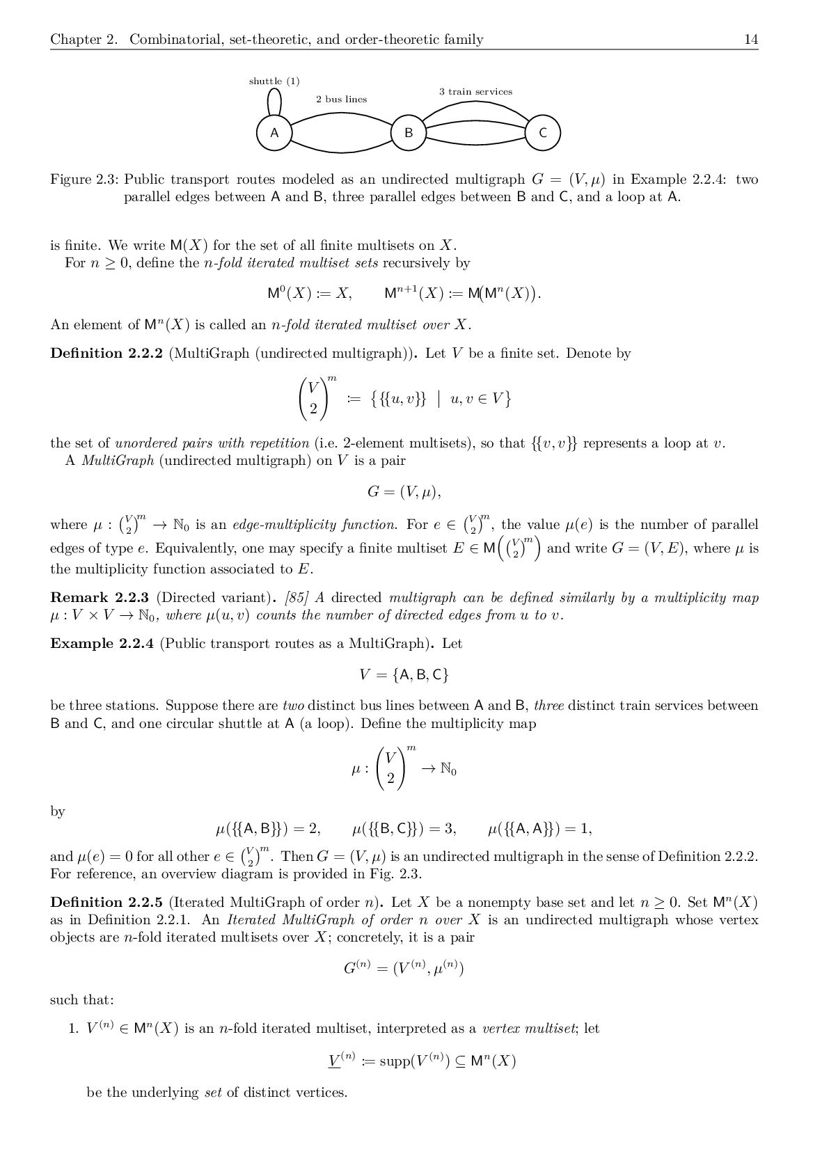
    A concise comparison of graphs, hypergraphs, n-superhypergraphs, and (m, n)-superhypergraphs. Structure Vertex domain Edge / incidence object What it captures (one line) Graph G = (V, E) V is a (finite) set of atomic vertices E ⊆ P∗ 2 (V ) = {{u, v} ⊆ V : u = v} (pairwise edges) Pairwise interactions only (bi- nary relations). Hypergraph H = (V, E) V is a (finite) set of atomic vertices E ⊆ P∗(V ) (hyperedges are nonempty subsets of V ) Multiway interactions among arbitrary-size groups. n- SuperHyperGraph SHG(n) = (V, E, ∂) V ⊆ P n(V0 ) (vertices are n-level set-valued ob- jects over a base set V0 ) E is a set of edge identifiers and ∂ : E → P∗(V ) (inci- dence among supervertices) Higher-order interactions and hierarchical/nested vertex se- mantics via iterated powersets. (m, n)- SuperHyperGraph SHG(m,n) = (V, E) V ⊆ Fm,n (S) = {f : Pm (S) → Pn (S)} (ver- tices are superhyperfunc- tions) ∅ = E ⊆ P(V )\{∅} (hyper- edges group such functions) Higher-order relations among operators between hierarchi- cal domains/codomains (con- textual constraints on maps). Define three functions f1 , f2 , f3 ∈ F2,1 (S) as follows. For any X ∈ P2 (S) = P(P(S)) (so X is a set of subsets of S), set f1 (X) := A∈X A, (the union of all subsets in X), f2 (X) := A∈X A, (with the convention ∅ = S), and f3 (X) := {a}, if {a} ∈ X, ∅, otherwise. Let the vertex set be the nonempty set of concrete (2, 1)-superhyperfunctions V = {f1 , f2 , f3 } ⊆ F2,1 (S). Define a nonempty family of hyperedges by E = E1 , E2 ⊆ P(V ) \ {∅}, E1 = {f1 , f2 }, E2 = {f2 , f3 }. Then SHG(2,1) = (V, E) is a concrete (2, 1)-SuperHyperGraph in the sense of Definition 2.1.9. Here E1 groups the “aggregation” super- hyperfunctions f1 (union) and f2 (intersection), while E2 groups f2 with the indicator-type superhyperfunction f3 , representing a different contextual relationship among superhyperfunctions. For reference, a comparison of graphs, hypergraphs, n-superhypergraphs, and (m, n)-superhypergraphs is provided in Table 2.2. 2.2 MultiGraph and Iterated MultiGraph A multigraph is a graph allowing parallel edges and loops; formally edges are a multiset with multiplicities between vertices possibly [72, 73, 74]. As extensions, concepts such as fuzzy multigraphs [75, 76, 77], bipartite multigraphs[78, 79], complete multigraphs[80, 81], neutrosophic multigraphs [72, 82], soft multigraphs[83], and directed multigraphs [84] are known. An iterated multigraph uses iterated multisets as vertex objects, so vertices themselves can be multisets nested to depth n recursively. Definition 2.2.1 (Finite multiset and iterated multiset). Let X be a set. A finite multiset on X is a function m : X → N0 whose support supp(m) := {x ∈ X | m(x) > 0}
  14. Chapter 2. Combinatorial, set-theoretic, and order-theoretic family 14 A B

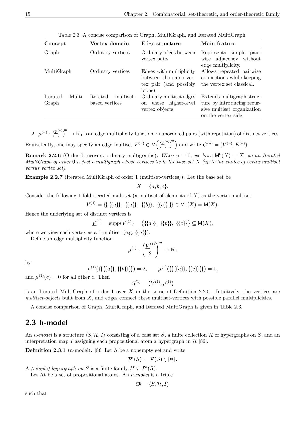
    C 2 bus lines 3 train services shuttle (1) Figure 2.3: Public transport routes modeled as an undirected multigraph G = (V, µ) in Example 2.2.4: two parallel edges between A and B, three parallel edges between B and C, and a loop at A. is finite. We write M(X) for the set of all finite multisets on X. For n ≥ 0, define the n-fold iterated multiset sets recursively by M0(X) := X, Mn+1(X) := M Mn(X) . An element of Mn(X) is called an n-fold iterated multiset over X. Definition 2.2.2 (MultiGraph (undirected multigraph)). Let V be a finite set. Denote by V 2 m := {{u, v}} u, v ∈ V the set of unordered pairs with repetition (i.e. 2-element multisets), so that {{v, v}} represents a loop at v. A MultiGraph (undirected multigraph) on V is a pair G = (V, µ), where µ : V 2 m → N0 is an edge-multiplicity function. For e ∈ V 2 m, the value µ(e) is the number of parallel edges of type e. Equivalently, one may specify a finite multiset E ∈ M V 2 m and write G = (V, E), where µ is the multiplicity function associated to E. Remark 2.2.3 (Directed variant). [85] A directed multigraph can be defined similarly by a multiplicity map µ : V × V → N0 , where µ(u, v) counts the number of directed edges from u to v. Example 2.2.4 (Public transport routes as a MultiGraph). Let V = {A, B, C} be three stations. Suppose there are two distinct bus lines between A and B, three distinct train services between B and C, and one circular shuttle at A (a loop). Define the multiplicity map µ : V 2 m → N0 by µ({{A, B}}) = 2, µ({{B, C}}) = 3, µ({{A, A}}) = 1, and µ(e) = 0 for all other e ∈ V 2 m. Then G = (V, µ) is an undirected multigraph in the sense of Definition 2.2.2. For reference, an overview diagram is provided in Fig. 2.3. Definition 2.2.5 (Iterated MultiGraph of order n). Let X be a nonempty base set and let n ≥ 0. Set Mn(X) as in Definition 2.2.1. An Iterated MultiGraph of order n over X is an undirected multigraph whose vertex objects are n-fold iterated multisets over X; concretely, it is a pair G(n) = (V (n), µ(n)) such that: 1. V (n) ∈ Mn(X) is an n-fold iterated multiset, interpreted as a vertex multiset; let V (n) := supp(V (n)) ⊆ Mn(X) be the underlying set of distinct vertices.
  15. 15 Chapter 2. Combinatorial, set-theoretic, and order-theoretic family Table 2.3:

    A concise comparison of Graph, MultiGraph, and Iterated MultiGraph. Concept Vertex domain Edge structure Main feature Graph Ordinary vertices Ordinary edges between vertex pairs Represents simple pair- wise adjacency without edge multiplicity. MultiGraph Ordinary vertices Edges with multiplicity between the same ver- tex pair (and possibly loops) Allows repeated pairwise connections while keeping the vertex set classical. Iterated Multi- Graph Iterated multiset- based vertices Ordinary multiset edges on those higher-level vertex objects Extends multigraph struc- ture by introducing recur- sive multiset organization on the vertex side. 2. µ(n) : V (n) 2 m → N0 is an edge-multiplicity function on unordered pairs (with repetition) of distinct vertices. Equivalently, one may specify an edge multiset E(n) ∈ M V (n) 2 m and write G(n) = (V (n), E(n)). Remark 2.2.6 (Order 0 recovers ordinary multigraphs). When n = 0, we have M0(X) = X, so an Iterated MultiGraph of order 0 is just a multigraph whose vertices lie in the base set X (up to the choice of vertex multiset versus vertex set). Example 2.2.7 (Iterated MultiGraph of order 1 (multiset-vertices)). Let the base set be X = {a, b, c}. Consider the following 1-fold iterated multiset (a multiset of elements of X) as the vertex multiset: V (1) = {{ {{a}}, {{a}}, {{b}}, {{c}} }} ∈ M1(X) = M(X). Hence the underlying set of distinct vertices is V (1) = supp(V (1)) = {{a}}, {{b}}, {{c}} ⊆ M(X), where we view each vertex as a 1-multiset (e.g. {{a}}). Define an edge-multiplicity function µ(1) : V (1) 2 m → N0 by µ(1)({{{{a}}, {{b}}}}) = 2, µ(1)({{{{a}}, {{c}}}}) = 1, and µ(1)(e) = 0 for all other e. Then G(1) = V (1), µ(1) is an Iterated MultiGraph of order 1 over X in the sense of Definition 2.2.5. Intuitively, the vertices are multiset-objects built from X, and edges connect these multiset-vertices with possible parallel multiplicities. A concise comparison of Graph, MultiGraph, and Iterated MultiGraph is given in Table 2.3. 2.3 h-model An h-model is a structure S, H, I consisting of a base set S, a finite collection H of hypergraphs on S, and an interpretation map I assigning each propositional atom a hypergraph in H [86]. Definition 2.3.1 (h-model). [86] Let S be a nonempty set and write P∗(S) := P(S) \ {∅}. A (simple) hypergraph on S is a finite family H ⊆ P∗(S). Let At be a set of propositional atoms. An h-model is a triple M = S, H, I such that
  16. Chapter 2. Combinatorial, set-theoretic, and order-theoretic family 16 1. H

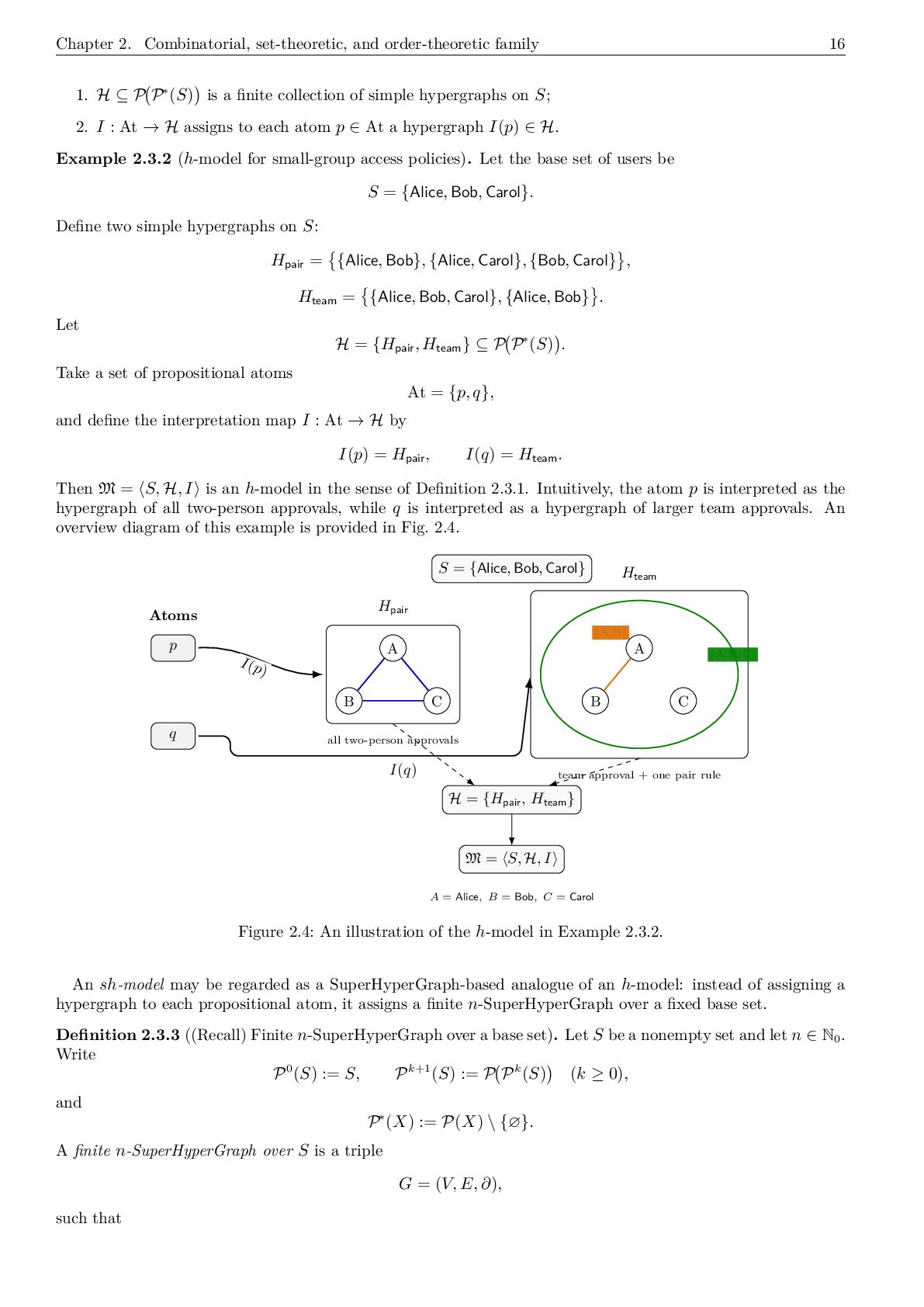
    ⊆ P P∗(S) is a finite collection of simple hypergraphs on S; 2. I : At → H assigns to each atom p ∈ At a hypergraph I(p) ∈ H. Example 2.3.2 (h-model for small-group access policies). Let the base set of users be S = {Alice, Bob, Carol}. Define two simple hypergraphs on S: Hpair = {Alice, Bob}, {Alice, Carol}, {Bob, Carol} , Hteam = {Alice, Bob, Carol}, {Alice, Bob} . Let H = {Hpair, Hteam} ⊆ P P∗(S) . Take a set of propositional atoms At = {p, q}, and define the interpretation map I : At → H by I(p) = Hpair, I(q) = Hteam. Then M = S, H, I is an h-model in the sense of Definition 2.3.1. Intuitively, the atom p is interpreted as the hypergraph of all two-person approvals, while q is interpreted as a hypergraph of larger team approvals. An overview diagram of this example is provided in Fig. 2.4. p q Atoms S = {Alice, Bob, Carol} A B C Hpair all two-person approvals A B C Hteam team approval + one pair rule {A, B, C} {A, B} I(p) I(q) H = {Hpair, Hteam} M = S, H, I A = Alice, B = Bob, C = Carol Figure 2.4: An illustration of the h-model in Example 2.3.2. An sh-model may be regarded as a SuperHyperGraph-based analogue of an h-model: instead of assigning a hypergraph to each propositional atom, it assigns a finite n-SuperHyperGraph over a fixed base set. Definition 2.3.3 ((Recall) Finite n-SuperHyperGraph over a base set). Let S be a nonempty set and let n ∈ N0 . Write P0(S) := S, Pk+1(S) := P Pk(S) (k ≥ 0), and P∗(X) := P(X) \ {∅}. A finite n-SuperHyperGraph over S is a triple G = (V, E, ∂), such that
  17. 17 Chapter 2. Combinatorial, set-theoretic, and order-theoretic family 1. V

    ⊆ Pn(S) is a finite set; 2. E is a finite set; 3. ∂ : E −→ P∗(V ) is a map. We denote by SHG n (S) the class of all finite n-SuperHyperGraphs over S. Definition 2.3.4 (sh-model). Let S be a nonempty set, let n ∈ N0 , and let At be a set of propositional atoms. An sh-model of level n is a quadruple M(n) = S, SH, I, n such that 1. SH ⊆ SHG n (S) is a finite collection of finite n-SuperHyperGraphs over S; 2. I : At −→ SH is an interpretation map assigning to each atom p ∈ At a member I(p) ∈ SH. Remark 2.3.5. If n = 0, then P0(S) = S, and each finite 0-SuperHyperGraph over S is simply a finite hypergraph written in incidence-map form. Hence an sh-model of level 0 reduces to a hypergraph-based model of the same general type as an h-model. Theorem 2.3.6 (Well-definedness of sh-models). Let S be a nonempty set, let n ∈ N0 , and let At be a set of propositional atoms. Suppose that SH ⊆ SHG n (S) is a finite family of finite n-SuperHyperGraphs over S, and let I : At → SH be any map. Then M(n) = S, SH, I, n is a well-defined sh-model in the sense of Definition 2.3.4. Proof. We verify the two clauses of Definition 2.3.4. Since n ∈ N0 and S = ∅, the iterated powerset Pn(S) is well-defined by recursion. Hence the notion of a finite n-SuperHyperGraph over S is meaningful by Definition 2.3.3. Therefore SHG n (S) is a well-defined class of objects, and the assumption SH ⊆ SHG n (S) means precisely that every member of SH is a finite n-SuperHyperGraph over S. By hypothesis, SH is finite, so condition (1) of Definition 2.3.4 holds. Next, the map I : At → SH is assumed to be a function. Hence for each propositional atom p ∈ At, there exists a unique value I(p) ∈ SH. Thus condition (2) of Definition 2.3.4 also holds. Therefore all constituents of M(n) = S, SH, I, n are well-defined and satisfy the required properties. Consequently, M(n) is a well-defined sh-model.
  18. Chapter 2. Combinatorial, set-theoretic, and order-theoretic family 18 2.4 Chain-Free

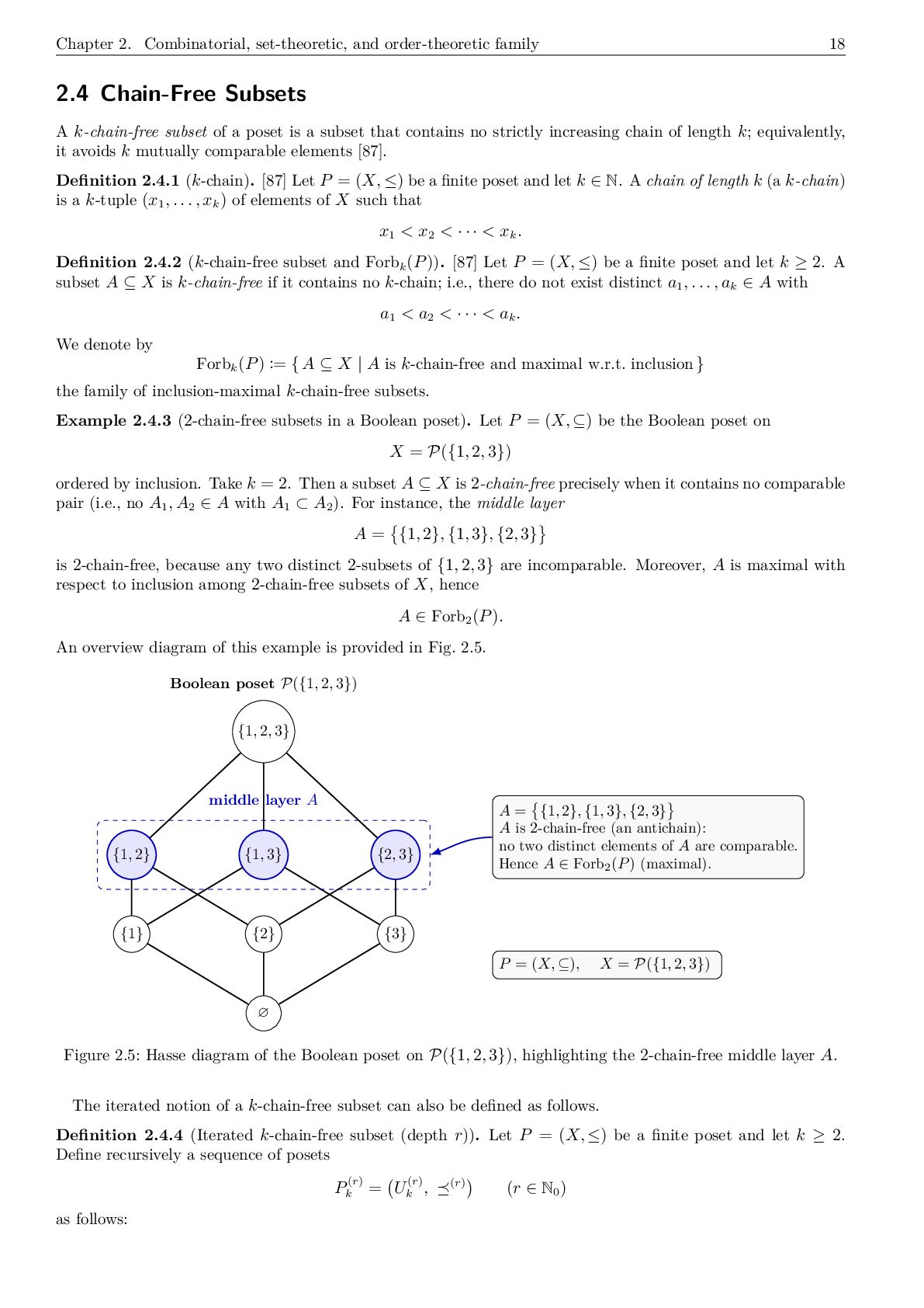
    Subsets A k-chain-free subset of a poset is a subset that contains no strictly increasing chain of length k; equivalently, it avoids k mutually comparable elements [87]. Definition 2.4.1 (k-chain). [87] Let P = (X, ≤) be a finite poset and let k ∈ N. A chain of length k (a k-chain) is a k-tuple (x1 , . . . , xk ) of elements of X such that x1 < x2 < · · · < xk . Definition 2.4.2 (k-chain-free subset and Forb k (P)). [87] Let P = (X, ≤) be a finite poset and let k ≥ 2. A subset A ⊆ X is k-chain-free if it contains no k-chain; i.e., there do not exist distinct a1 , . . . , ak ∈ A with a1 < a2 < · · · < ak . We denote by Forb k (P) := { A ⊆ X | A is k-chain-free and maximal w.r.t. inclusion } the family of inclusion-maximal k-chain-free subsets. Example 2.4.3 (2-chain-free subsets in a Boolean poset). Let P = (X, ⊆) be the Boolean poset on X = P({1, 2, 3}) ordered by inclusion. Take k = 2. Then a subset A ⊆ X is 2-chain-free precisely when it contains no comparable pair (i.e., no A1 , A2 ∈ A with A1 ⊂ A2 ). For instance, the middle layer A = {1, 2}, {1, 3}, {2, 3} is 2-chain-free, because any two distinct 2-subsets of {1, 2, 3} are incomparable. Moreover, A is maximal with respect to inclusion among 2-chain-free subsets of X, hence A ∈ Forb 2 (P). An overview diagram of this example is provided in Fig. 2.5. ∅ {1} {2} {3} {1, 2} {1, 3} {2, 3} {1, 2, 3} middle layer A A = {1, 2}, {1, 3}, {2, 3} A is 2-chain-free (an antichain): no two distinct elements of A are comparable. Hence A ∈ Forb2 (P) (maximal). P = (X, ⊆), X = P({1, 2, 3}) Boolean poset P({1, 2, 3}) Figure 2.5: Hasse diagram of the Boolean poset on P({1, 2, 3}), highlighting the 2-chain-free middle layer A. The iterated notion of a k-chain-free subset can also be defined as follows. Definition 2.4.4 (Iterated k-chain-free subset (depth r)). Let P = (X, ≤) be a finite poset and let k ≥ 2. Define recursively a sequence of posets P(r) k = U(r) k , (r) (r ∈ N0 ) as follows:
  19. 19 Chapter 2. Combinatorial, set-theoretic, and order-theoretic family 1. (Depth

    0) Set U(0) k := X and (0):=≤. 2. (Depth r + 1) Having defined P(r) k = (U(r) k , (r)), let U(r+1) k := A ⊆ U(r) k A is k-chain-free in the poset (U(r) k , (r)) , and equip U(r+1) k with the inclusion order A (r+1) B :⇐⇒ A ⊆ B (A, B ∈ U(r+1) k ). An element of U(r) k is called an iterated k-chain-free subset of depth r (over P). Equivalently, it is a “k-chain-free set of k-chain-free sets of · · · of k-chain-free sets” (r iterations), where the first iteration uses ≤ on X, and higher iterations use inclusion. Remark 2.4.5 (Maximal (iterated) k-chain-free families). If one prefers inclusion-maximal objects at each depth, define Forb(r) k (P) := A ∈ U(r) k A is maximal in (U(r) k , ⊆) (r ≥ 1), so Forb(1) k (P) coincides with the family of maximal k-chain-free subsets of P. Example 2.4.6 (An iterated 2-chain-free subset of depth 2). Let P = (X, ⊆) again be the Boolean poset on X = P({1, 2, 3}), and let k = 2. As in Example 2.4.3, elements of U(1) 2 are 2-chain-free families of subsets of {1, 2, 3}. Consider the following three maximal 2-chain-free families (each is an antichain in X): A1 = {1}, {2}, {3} , A2 = {1, 2}, {1, 3}, {2, 3} , A3 = ∅, {1, 2, 3} . Each Ai is 2-chain-free in (X, ⊆), so A1 , A2 , A3 ∈ U(1) 2 . Now form a depth-2 object (a set of 2-chain-free sets) by B = {A1 , A2 } ⊆ U(1) 2 . Since U(1) 2 is ordered by inclusion of families, and A1 and A2 are incomparable (neither is a subset of the other), the set B contains no 2-chain in the poset (U(1) 2 , ⊆). Hence B is 2-chain-free in (U(1) 2 , ⊆), and therefore B ∈ U(2) 2 . Thus B is an iterated 2-chain-free subset of depth 2 in the sense of Definition 2.4.4. Theorem 2.4.7 (Well-definedness of iterated k-chain-free subsets). Let P = (X, ≤) be a finite poset and let k ≥ 2. Define P(r) k = (U(r) k , (r)) recursively as in Definition 2.4.4. Then for every r ∈ N0 : (i) U(r) k is a well-defined finite set, and in particular U(r+1) k ⊆ P U(r) k . (ii) (r) is a well-defined partial order on U(r) k ; hence P(r) k is a finite poset. Consequently, the phrase “iterated k-chain-free subset of depth r” is well-defined. Proof. We argue by induction on r. Base case r = 0. By definition, U(0) k = X and (0)=≤. Since P = (X, ≤) is assumed to be a finite poset, U(0) k is a finite set and (0) is a partial order on it. Thus P(0) k is well-defined as a finite poset. Inductive step. Assume that for some r ∈ N0 the structure P(r) k = (U(r) k , (r)) is a well-defined finite poset. We must show that P(r+1) k = (U(r+1) k , (r+1)) is a well-defined finite poset. (i) U(r+1) k is well-defined and finite. Because (U(r) k , (r)) is a poset by the induction hypothesis, the notion “A is k-chain-free in (U(r) k , (r))” is meaningful; explicitly, A ⊆ U(r) k is k-chain-free if there do not exist elements x1 , . . . , xk ∈ A such that x1 ≺(r) x2 ≺(r) · · · ≺(r) xk . Hence the specification U(r+1) k = { A ⊆ U(r) k | A is k-chain-free in (U(r) k , (r)) }
  20. Chapter 2. Combinatorial, set-theoretic, and order-theoretic family 20 defines a

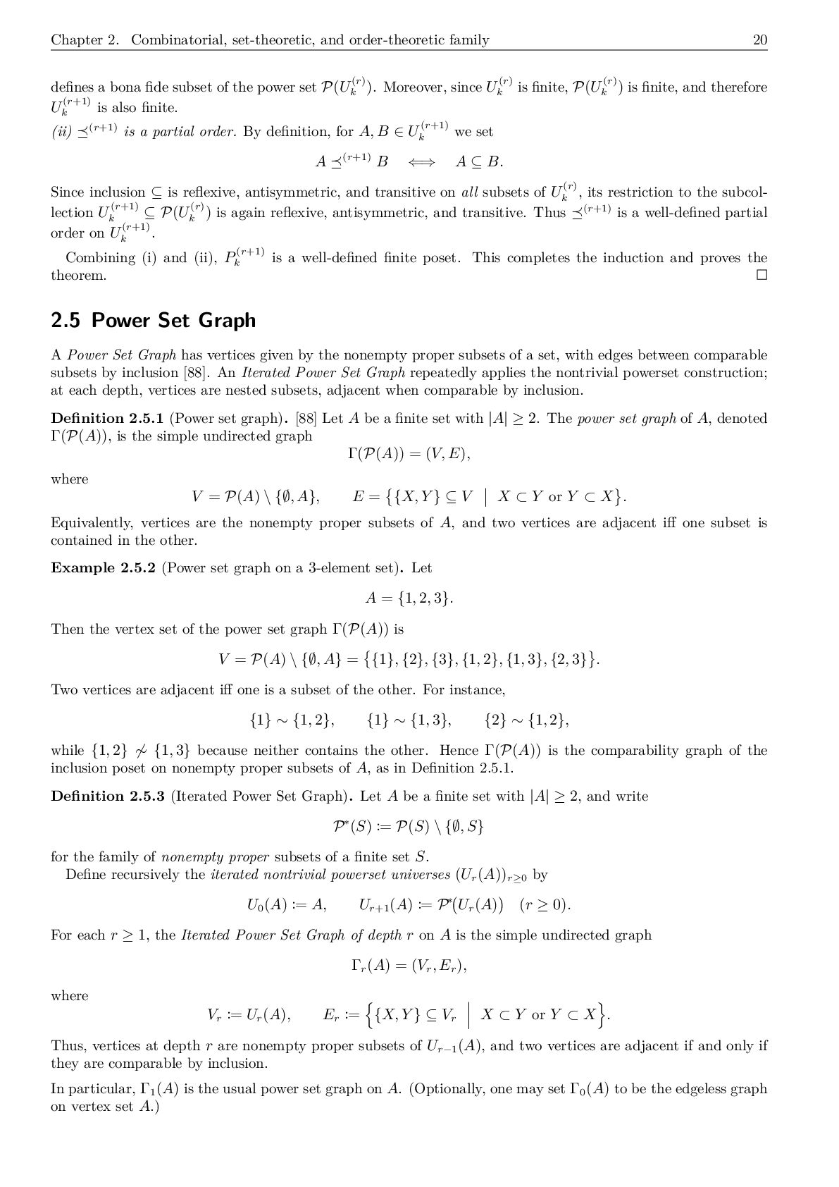
    bona fide subset of the power set P(U(r) k ). Moreover, since U(r) k is finite, P(U(r) k ) is finite, and therefore U(r+1) k is also finite. (ii) (r+1) is a partial order. By definition, for A, B ∈ U(r+1) k we set A (r+1) B ⇐⇒ A ⊆ B. Since inclusion ⊆ is reflexive, antisymmetric, and transitive on all subsets of U(r) k , its restriction to the subcol- lection U(r+1) k ⊆ P(U(r) k ) is again reflexive, antisymmetric, and transitive. Thus (r+1) is a well-defined partial order on U(r+1) k . Combining (i) and (ii), P(r+1) k is a well-defined finite poset. This completes the induction and proves the theorem. 2.5 Power Set Graph A Power Set Graph has vertices given by the nonempty proper subsets of a set, with edges between comparable subsets by inclusion [88]. An Iterated Power Set Graph repeatedly applies the nontrivial powerset construction; at each depth, vertices are nested subsets, adjacent when comparable by inclusion. Definition 2.5.1 (Power set graph). [88] Let A be a finite set with |A| ≥ 2. The power set graph of A, denoted Γ(P(A)), is the simple undirected graph Γ(P(A)) = (V, E), where V = P(A) \ {∅, A}, E = {X, Y } ⊆ V X ⊂ Y or Y ⊂ X . Equivalently, vertices are the nonempty proper subsets of A, and two vertices are adjacent iff one subset is contained in the other. Example 2.5.2 (Power set graph on a 3-element set). Let A = {1, 2, 3}. Then the vertex set of the power set graph Γ(P(A)) is V = P(A) \ {∅, A} = {1}, {2}, {3}, {1, 2}, {1, 3}, {2, 3} . Two vertices are adjacent iff one is a subset of the other. For instance, {1} ∼ {1, 2}, {1} ∼ {1, 3}, {2} ∼ {1, 2}, while {1, 2} ∼ {1, 3} because neither contains the other. Hence Γ(P(A)) is the comparability graph of the inclusion poset on nonempty proper subsets of A, as in Definition 2.5.1. Definition 2.5.3 (Iterated Power Set Graph). Let A be a finite set with |A| ≥ 2, and write P∗(S) := P(S) \ {∅, S} for the family of nonempty proper subsets of a finite set S. Define recursively the iterated nontrivial powerset universes (Ur (A))r≥0 by U0 (A) := A, Ur+1 (A) := P∗ Ur (A) (r ≥ 0). For each r ≥ 1, the Iterated Power Set Graph of depth r on A is the simple undirected graph Γr (A) = (Vr , Er ), where Vr := Ur (A), Er := {X, Y } ⊆ Vr X ⊂ Y or Y ⊂ X . Thus, vertices at depth r are nonempty proper subsets of Ur−1 (A), and two vertices are adjacent if and only if they are comparable by inclusion. In particular, Γ1 (A) is the usual power set graph on A. (Optionally, one may set Γ0 (A) to be the edgeless graph on vertex set A.)
  21. 21 Chapter 2. Combinatorial, set-theoretic, and order-theoretic family Example 2.5.4

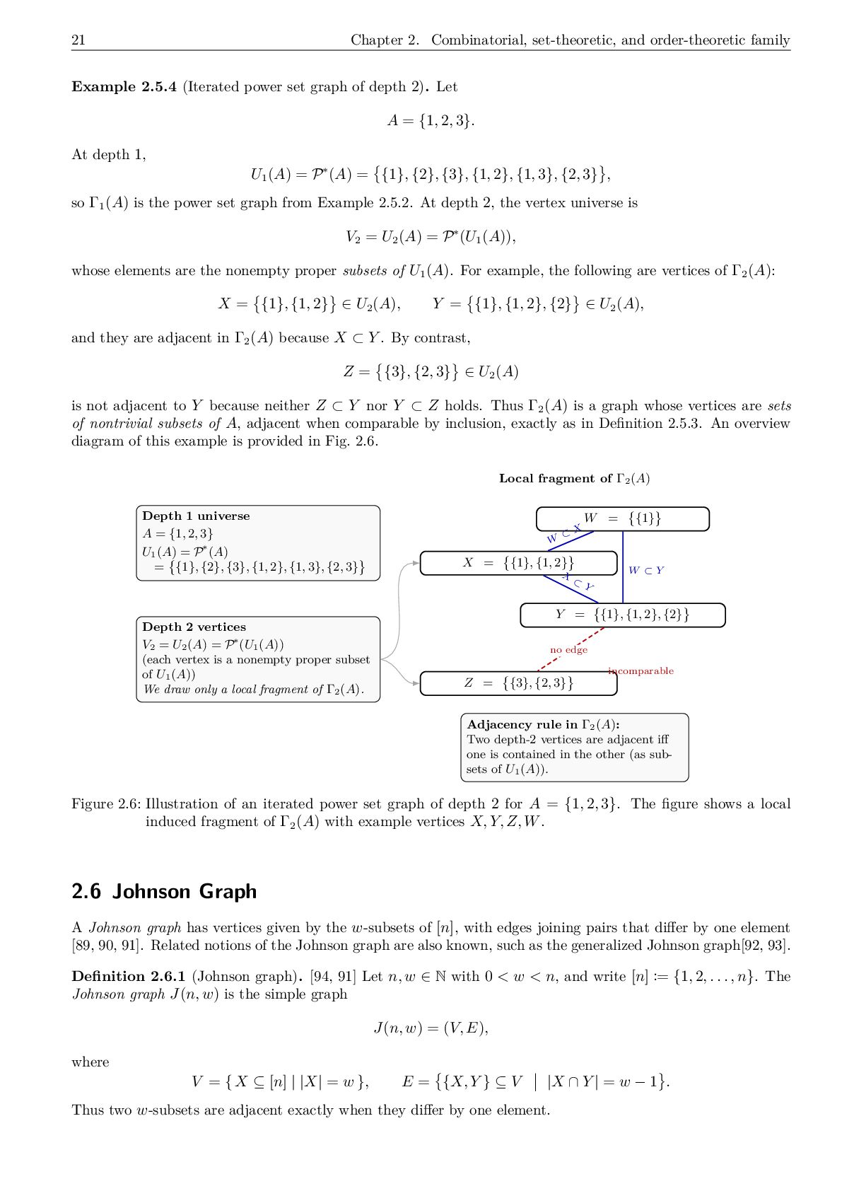
    (Iterated power set graph of depth 2). Let A = {1, 2, 3}. At depth 1, U1 (A) = P∗(A) = {1}, {2}, {3}, {1, 2}, {1, 3}, {2, 3} , so Γ1 (A) is the power set graph from Example 2.5.2. At depth 2, the vertex universe is V2 = U2 (A) = P∗(U1 (A)), whose elements are the nonempty proper subsets of U1 (A). For example, the following are vertices of Γ2 (A): X = {1}, {1, 2} ∈ U2 (A), Y = {1}, {1, 2}, {2} ∈ U2 (A), and they are adjacent in Γ2 (A) because X ⊂ Y . By contrast, Z = {3}, {2, 3} ∈ U2 (A) is not adjacent to Y because neither Z ⊂ Y nor Y ⊂ Z holds. Thus Γ2 (A) is a graph whose vertices are sets of nontrivial subsets of A, adjacent when comparable by inclusion, exactly as in Definition 2.5.3. An overview diagram of this example is provided in Fig. 2.6. Depth 1 universe A = {1, 2, 3} U1 (A) = P∗(A) = { {1}, {2}, {3}, {1, 2}, {1, 3}, {2, 3} } Depth 2 vertices V2 = U2 (A) = P∗(U1 (A)) (each vertex is a nonempty proper subset of U1 (A)) We draw only a local fragment of Γ2 (A). Local fragment of Γ2 (A) X = { {1}, {1, 2} } Y = { {1}, {1, 2}, {2} } Z = { {3}, {2, 3} } W = { {1} } X ⊂ Y W ⊂ Y W ⊂ X no edge incomparable Adjacency rule in Γ2 (A): Two depth-2 vertices are adjacent iff one is contained in the other (as sub- sets of U1 (A)). Figure 2.6: Illustration of an iterated power set graph of depth 2 for A = {1, 2, 3}. The figure shows a local induced fragment of Γ2 (A) with example vertices X, Y, Z, W. 2.6 Johnson Graph A Johnson graph has vertices given by the w-subsets of [n], with edges joining pairs that differ by one element [89, 90, 91]. Related notions of the Johnson graph are also known, such as the generalized Johnson graph[92, 93]. Definition 2.6.1 (Johnson graph). [94, 91] Let n, w ∈ N with 0 < w < n, and write [n] := {1, 2, . . . , n}. The Johnson graph J(n, w) is the simple graph J(n, w) = (V, E), where V = { X ⊆ [n] | |X| = w }, E = {X, Y } ⊆ V |X ∩ Y | = w − 1 . Thus two w-subsets are adjacent exactly when they differ by one element.
  22. Chapter 2. Combinatorial, set-theoretic, and order-theoretic family 22 Example 2.6.2

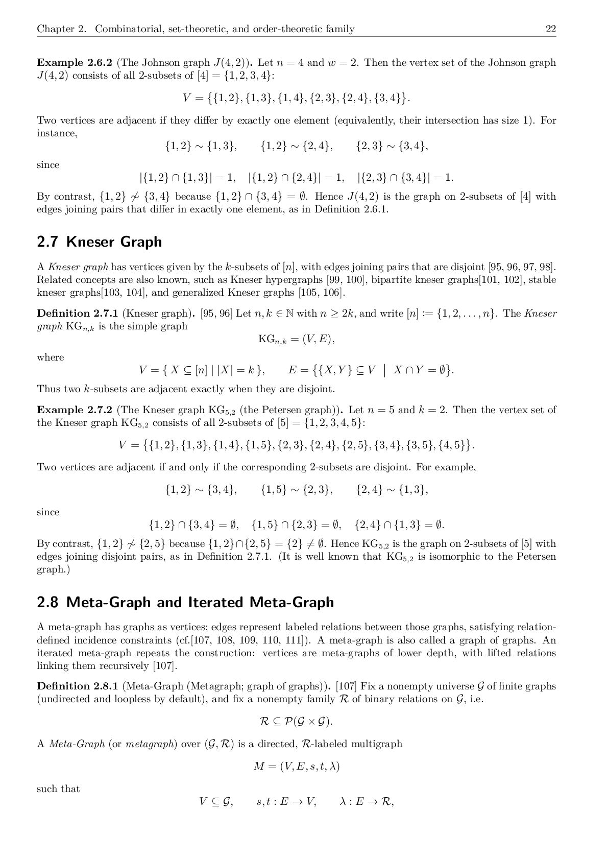
    (The Johnson graph J(4, 2)). Let n = 4 and w = 2. Then the vertex set of the Johnson graph J(4, 2) consists of all 2-subsets of [4] = {1, 2, 3, 4}: V = {1, 2}, {1, 3}, {1, 4}, {2, 3}, {2, 4}, {3, 4} . Two vertices are adjacent if they differ by exactly one element (equivalently, their intersection has size 1). For instance, {1, 2} ∼ {1, 3}, {1, 2} ∼ {2, 4}, {2, 3} ∼ {3, 4}, since |{1, 2} ∩ {1, 3}| = 1, |{1, 2} ∩ {2, 4}| = 1, |{2, 3} ∩ {3, 4}| = 1. By contrast, {1, 2} ∼ {3, 4} because {1, 2} ∩ {3, 4} = ∅. Hence J(4, 2) is the graph on 2-subsets of [4] with edges joining pairs that differ in exactly one element, as in Definition 2.6.1. 2.7 Kneser Graph A Kneser graph has vertices given by the k-subsets of [n], with edges joining pairs that are disjoint [95, 96, 97, 98]. Related concepts are also known, such as Kneser hypergraphs [99, 100], bipartite kneser graphs[101, 102], stable kneser graphs[103, 104], and generalized Kneser graphs [105, 106]. Definition 2.7.1 (Kneser graph). [95, 96] Let n, k ∈ N with n ≥ 2k, and write [n] := {1, 2, . . . , n}. The Kneser graph KG n,k is the simple graph KG n,k = (V, E), where V = { X ⊆ [n] | |X| = k }, E = {X, Y } ⊆ V X ∩ Y = ∅ . Thus two k-subsets are adjacent exactly when they are disjoint. Example 2.7.2 (The Kneser graph KG 5,2 (the Petersen graph)). Let n = 5 and k = 2. Then the vertex set of the Kneser graph KG 5,2 consists of all 2-subsets of [5] = {1, 2, 3, 4, 5}: V = {1, 2}, {1, 3}, {1, 4}, {1, 5}, {2, 3}, {2, 4}, {2, 5}, {3, 4}, {3, 5}, {4, 5} . Two vertices are adjacent if and only if the corresponding 2-subsets are disjoint. For example, {1, 2} ∼ {3, 4}, {1, 5} ∼ {2, 3}, {2, 4} ∼ {1, 3}, since {1, 2} ∩ {3, 4} = ∅, {1, 5} ∩ {2, 3} = ∅, {2, 4} ∩ {1, 3} = ∅. By contrast, {1, 2} ∼ {2, 5} because {1, 2}∩{2, 5} = {2} = ∅. Hence KG 5,2 is the graph on 2-subsets of [5] with edges joining disjoint pairs, as in Definition 2.7.1. (It is well known that KG 5,2 is isomorphic to the Petersen graph.) 2.8 Meta-Graph and Iterated Meta-Graph A meta-graph has graphs as vertices; edges represent labeled relations between those graphs, satisfying relation- defined incidence constraints (cf.[107, 108, 109, 110, 111]). A meta-graph is also called a graph of graphs. An iterated meta-graph repeats the construction: vertices are meta-graphs of lower depth, with lifted relations linking them recursively [107]. Definition 2.8.1 (Meta-Graph (Metagraph; graph of graphs)). [107] Fix a nonempty universe G of finite graphs (undirected and loopless by default), and fix a nonempty family R of binary relations on G, i.e. R ⊆ P(G × G). A Meta-Graph (or metagraph) over (G, R) is a directed, R-labeled multigraph M = (V, E, s, t, λ) such that V ⊆ G, s, t : E → V, λ : E → R,
  23. 23 Chapter 2. Combinatorial, set-theoretic, and order-theoretic family and the

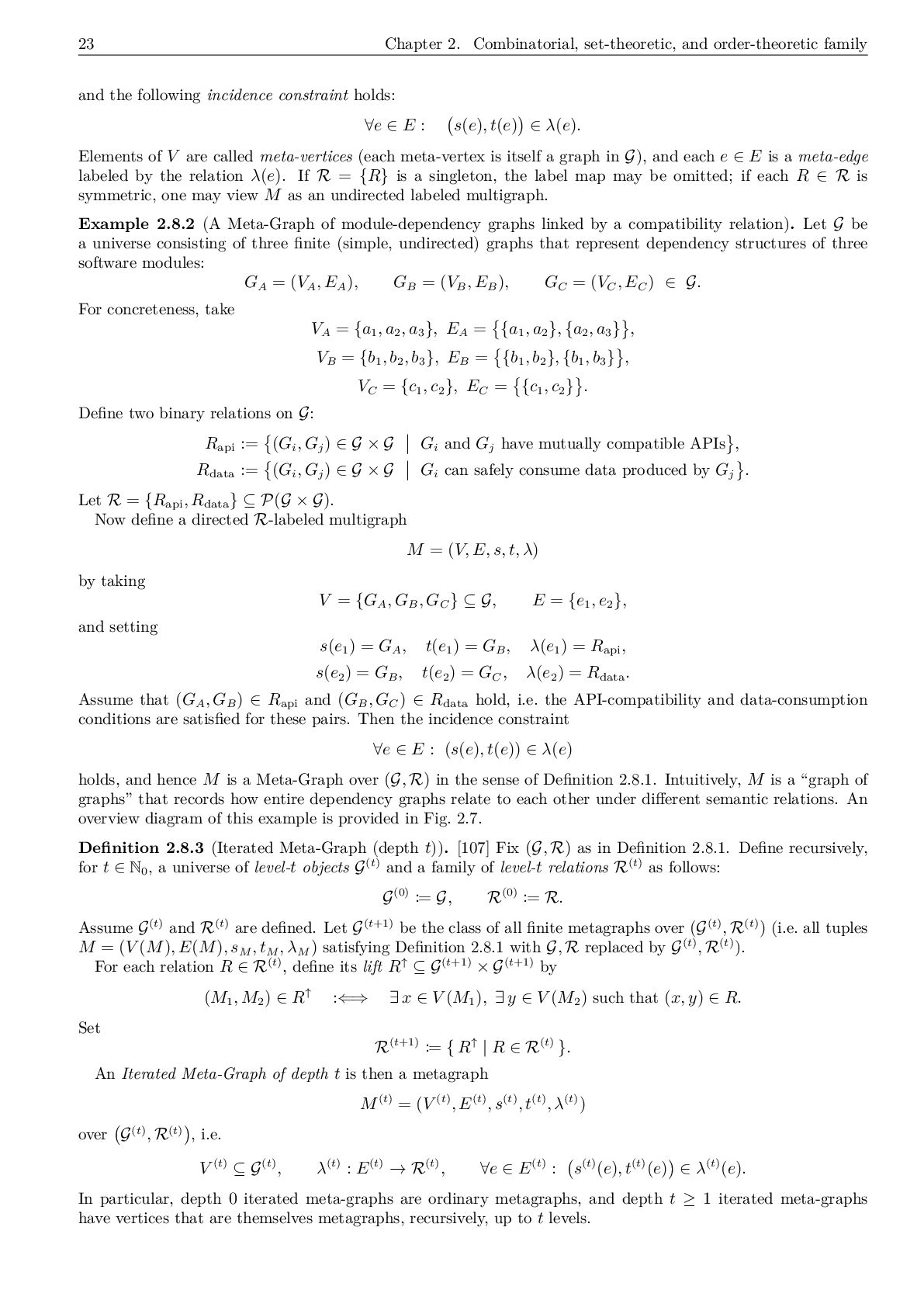
    following incidence constraint holds: ∀e ∈ E : s(e), t(e) ∈ λ(e). Elements of V are called meta-vertices (each meta-vertex is itself a graph in G), and each e ∈ E is a meta-edge labeled by the relation λ(e). If R = {R} is a singleton, the label map may be omitted; if each R ∈ R is symmetric, one may view M as an undirected labeled multigraph. Example 2.8.2 (A Meta-Graph of module-dependency graphs linked by a compatibility relation). Let G be a universe consisting of three finite (simple, undirected) graphs that represent dependency structures of three software modules: GA = (VA , EA ), GB = (VB , EB ), GC = (VC , EC ) ∈ G. For concreteness, take VA = {a1 , a2 , a3 }, EA = {a1 , a2 }, {a2 , a3 } , VB = {b1 , b2 , b3 }, EB = {b1 , b2 }, {b1 , b3 } , VC = {c1 , c2 }, EC = {c1 , c2 } . Define two binary relations on G: Rapi := (Gi , Gj ) ∈ G × G Gi and Gj have mutually compatible APIs , Rdata := (Gi , Gj ) ∈ G × G Gi can safely consume data produced by Gj . Let R = {Rapi, Rdata} ⊆ P(G × G). Now define a directed R-labeled multigraph M = (V, E, s, t, λ) by taking V = {GA , GB , GC } ⊆ G, E = {e1 , e2 }, and setting s(e1 ) = GA , t(e1 ) = GB , λ(e1 ) = Rapi, s(e2 ) = GB , t(e2 ) = GC , λ(e2 ) = Rdata. Assume that (GA , GB ) ∈ Rapi and (GB , GC ) ∈ Rdata hold, i.e. the API-compatibility and data-consumption conditions are satisfied for these pairs. Then the incidence constraint ∀e ∈ E : (s(e), t(e)) ∈ λ(e) holds, and hence M is a Meta-Graph over (G, R) in the sense of Definition 2.8.1. Intuitively, M is a “graph of graphs” that records how entire dependency graphs relate to each other under different semantic relations. An overview diagram of this example is provided in Fig. 2.7. Definition 2.8.3 (Iterated Meta-Graph (depth t)). [107] Fix (G, R) as in Definition 2.8.1. Define recursively, for t ∈ N0 , a universe of level-t objects G(t) and a family of level-t relations R(t) as follows: G(0) := G, R(0) := R. Assume G(t) and R(t) are defined. Let G(t+1) be the class of all finite metagraphs over (G(t), R(t)) (i.e. all tuples M = (V (M), E(M), sM , tM , λM ) satisfying Definition 2.8.1 with G, R replaced by G(t), R(t)). For each relation R ∈ R(t), define its lift R↑ ⊆ G(t+1) × G(t+1) by (M1 , M2 ) ∈ R↑ :⇐⇒ ∃ x ∈ V (M1 ), ∃ y ∈ V (M2 ) such that (x, y) ∈ R. Set R(t+1) := { R↑ | R ∈ R(t) }. An Iterated Meta-Graph of depth t is then a metagraph M(t) = (V (t), E(t), s(t), t(t), λ(t)) over G(t), R(t) , i.e. V (t) ⊆ G(t), λ(t) : E(t) → R(t), ∀e ∈ E(t) : s(t)(e), t(t)(e) ∈ λ(t)(e). In particular, depth 0 iterated meta-graphs are ordinary metagraphs, and depth t ≥ 1 iterated meta-graphs have vertices that are themselves metagraphs, recursively, up to t levels.
  24. Chapter 2. Combinatorial, set-theoretic, and order-theoretic family 24 GA GB

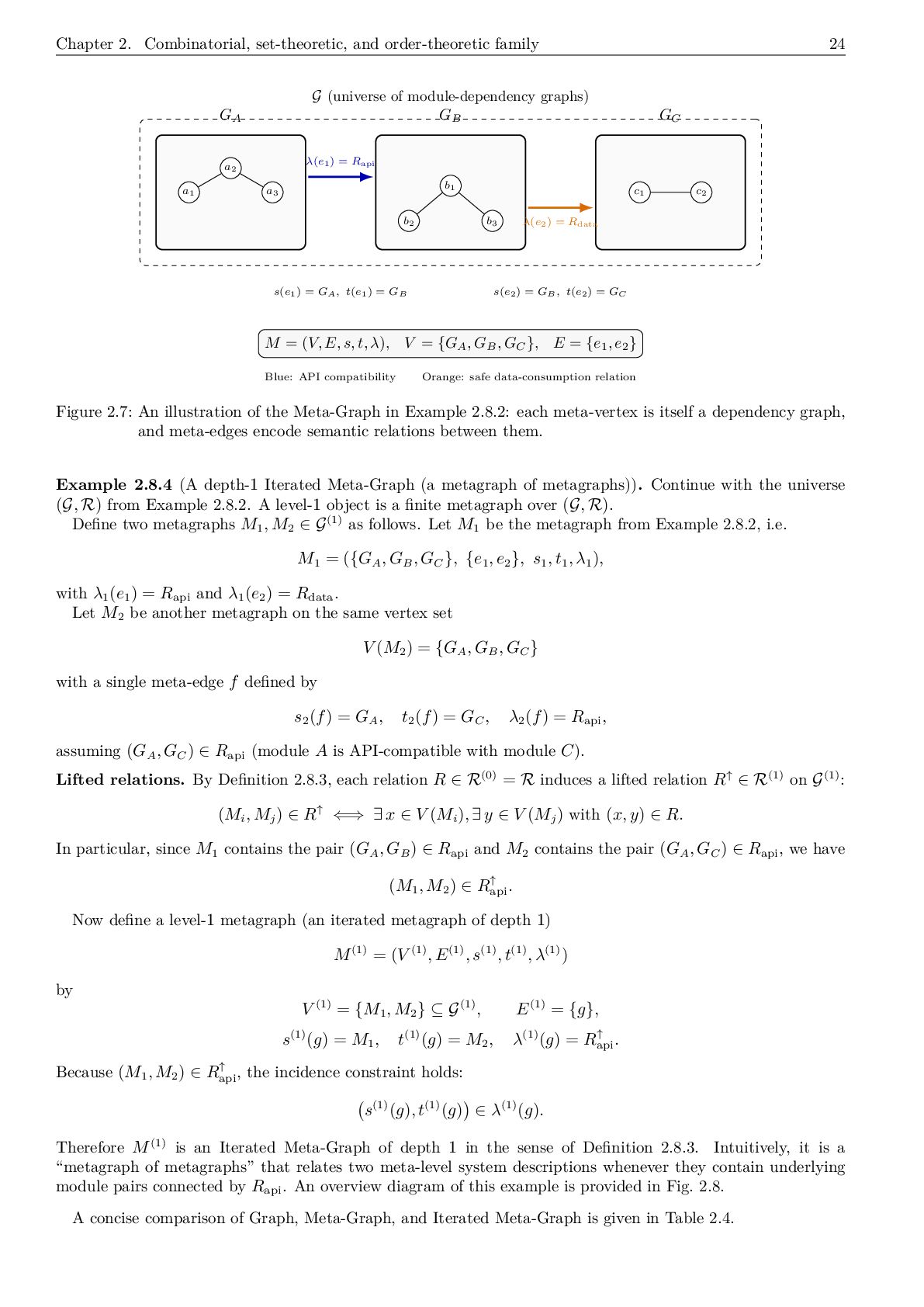
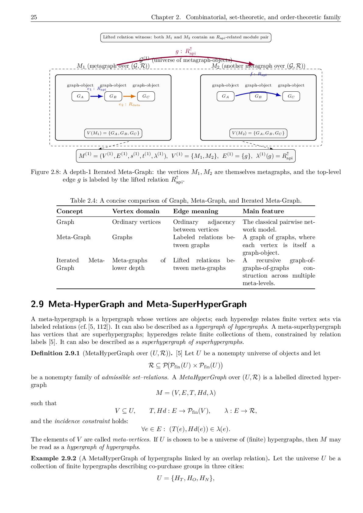
    GC a1 a2 a3 b1 b2 b3 c1 c2 λ(e1) = Rapi λ(e2) = Rdata s(e1) = GA, t(e1) = GB s(e2) = GB, t(e2) = GC G (universe of module-dependency graphs) M = (V, E, s, t, λ), V = {GA , GB , GC }, E = {e1 , e2 } Blue: API compatibility Orange: safe data-consumption relation Figure 2.7: An illustration of the Meta-Graph in Example 2.8.2: each meta-vertex is itself a dependency graph, and meta-edges encode semantic relations between them. Example 2.8.4 (A depth-1 Iterated Meta-Graph (a metagraph of metagraphs)). Continue with the universe (G, R) from Example 2.8.2. A level-1 object is a finite metagraph over (G, R). Define two metagraphs M1 , M2 ∈ G(1) as follows. Let M1 be the metagraph from Example 2.8.2, i.e. M1 = ({GA , GB , GC }, {e1 , e2 }, s1 , t1 , λ1 ), with λ1 (e1 ) = Rapi and λ1 (e2 ) = Rdata . Let M2 be another metagraph on the same vertex set V (M2 ) = {GA , GB , GC } with a single meta-edge f defined by s2 (f) = GA , t2 (f) = GC , λ2 (f) = Rapi, assuming (GA , GC ) ∈ Rapi (module A is API-compatible with module C). Lifted relations. By Definition 2.8.3, each relation R ∈ R(0) = R induces a lifted relation R↑ ∈ R(1) on G(1): (Mi , Mj ) ∈ R↑ ⇐⇒ ∃ x ∈ V (Mi ), ∃ y ∈ V (Mj ) with (x, y) ∈ R. In particular, since M1 contains the pair (GA , GB ) ∈ Rapi and M2 contains the pair (GA , GC ) ∈ Rapi , we have (M1 , M2 ) ∈ R↑ api . Now define a level-1 metagraph (an iterated metagraph of depth 1) M(1) = (V (1), E(1), s(1), t(1), λ(1)) by V (1) = {M1 , M2 } ⊆ G(1), E(1) = {g}, s(1)(g) = M1 , t(1)(g) = M2 , λ(1)(g) = R↑ api . Because (M1 , M2 ) ∈ R↑ api , the incidence constraint holds: s(1)(g), t(1)(g) ∈ λ(1)(g). Therefore M(1) is an Iterated Meta-Graph of depth 1 in the sense of Definition 2.8.3. Intuitively, it is a “metagraph of metagraphs” that relates two meta-level system descriptions whenever they contain underlying module pairs connected by Rapi . An overview diagram of this example is provided in Fig. 2.8. A concise comparison of Graph, Meta-Graph, and Iterated Meta-Graph is given in Table 2.4.
  25. 25 Chapter 2. Combinatorial, set-theoretic, and order-theoretic family M1 (metagraph

    over (G, R)) GA GB GC graph-object graph-object graph-object e1 : Rapi e2 : Rdata V (M1) = {GA, GB, GC } M2 (another metagraph over (G, R)) GA GB GC graph-object graph-object graph-object f : Rapi V (M2) = {GA, GB, GC } g : R↑ api Lifted relation witness: both M1 and M2 contain an Rapi -related module pair M(1) = (V (1), E(1), s(1), t(1), λ(1)), V (1) = {M1 , M2 }, E(1) = {g}, λ(1)(g) = R↑ api G(1) (universe of metagraph-objects) Figure 2.8: A depth-1 Iterated Meta-Graph: the vertices M1 , M2 are themselves metagraphs, and the top-level edge g is labeled by the lifted relation R↑ api . Table 2.4: A concise comparison of Graph, Meta-Graph, and Iterated Meta-Graph. Concept Vertex domain Edge meaning Main feature Graph Ordinary vertices Ordinary adjacency between vertices The classical pairwise net- work model. Meta-Graph Graphs Labeled relations be- tween graphs A graph of graphs, where each vertex is itself a graph-object. Iterated Meta- Graph Meta-graphs of lower depth Lifted relations be- tween meta-graphs A recursive graph-of- graphs-of-graphs con- struction across multiple meta-levels. 2.9 Meta-HyperGraph and Meta-SuperHyperGraph A meta-hypergraph is a hypergraph whose vertices are objects; each hyperedge relates finite vertex sets via labeled relations (cf. [5, 112]). It can also be described as a hypergraph of hypergraphs. A meta-superhypergraph has vertices that are superhypergraphs; hyperedges relate finite collections of them, constrained by relation labels [5]. It can also be described as a superhypergraph of superhypergraphs. Definition 2.9.1 (MetaHyperGraph over (U, R)). [5] Let U be a nonempty universe of objects and let R ⊆ P Pfin(U) × Pfin(U) be a nonempty family of admissible set–relations. A MetaHyperGraph over (U, R) is a labelled directed hyper- graph M = (V, E, T, Hd, λ) such that V ⊆ U, T, Hd : E → Pfin(V ), λ : E → R, and the incidence constraint holds: ∀e ∈ E : (T(e), Hd(e)) ∈ λ(e). The elements of V are called meta-vertices. If U is chosen to be a universe of (finite) hypergraphs, then M may be read as a hypergraph of hypergraphs. Example 2.9.2 (A MetaHyperGraph of hypergraphs linked by an overlap relation). Let the universe U be a collection of finite hypergraphs describing co-purchase groups in three cities: U = {HT , HO , HN },
  26. Chapter 2. Combinatorial, set-theoretic, and order-theoretic family 26 where each

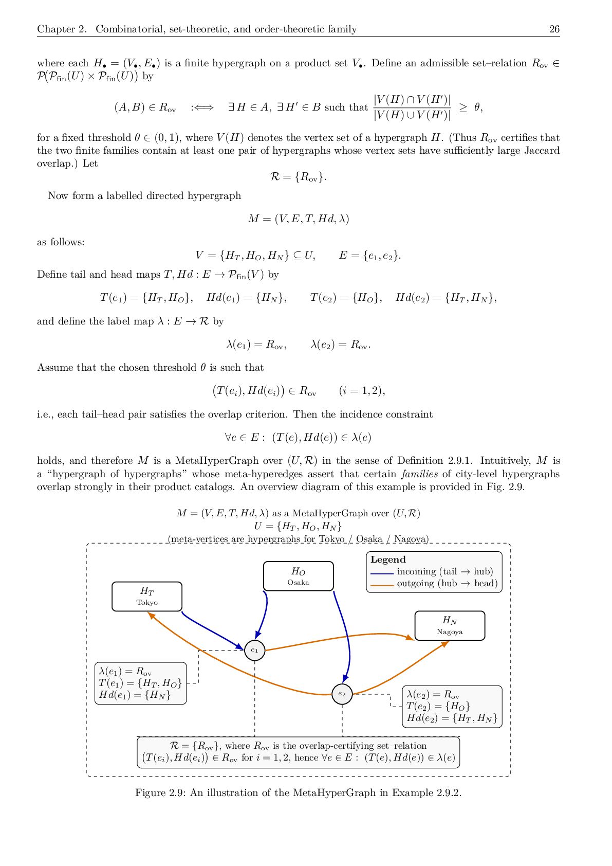
    H• = (V• , E• ) is a finite hypergraph on a product set V• . Define an admissible set–relation Rov ∈ P Pfin(U) × Pfin(U) by (A, B) ∈ Rov :⇐⇒ ∃ H ∈ A, ∃ H ∈ B such that |V (H) ∩ V (H )| |V (H) ∪ V (H )| ≥ θ, for a fixed threshold θ ∈ (0, 1), where V (H) denotes the vertex set of a hypergraph H. (Thus Rov certifies that the two finite families contain at least one pair of hypergraphs whose vertex sets have sufficiently large Jaccard overlap.) Let R = {Rov}. Now form a labelled directed hypergraph M = (V, E, T, Hd, λ) as follows: V = {HT , HO , HN } ⊆ U, E = {e1 , e2 }. Define tail and head maps T, Hd : E → Pfin(V ) by T(e1 ) = {HT , HO }, Hd(e1 ) = {HN }, T(e2 ) = {HO }, Hd(e2 ) = {HT , HN }, and define the label map λ : E → R by λ(e1 ) = Rov, λ(e2 ) = Rov. Assume that the chosen threshold θ is such that T(ei ), Hd(ei ) ∈ Rov (i = 1, 2), i.e., each tail–head pair satisfies the overlap criterion. Then the incidence constraint ∀e ∈ E : (T(e), Hd(e)) ∈ λ(e) holds, and therefore M is a MetaHyperGraph over (U, R) in the sense of Definition 2.9.1. Intuitively, M is a “hypergraph of hypergraphs” whose meta-hyperedges assert that certain families of city-level hypergraphs overlap strongly in their product catalogs. An overview diagram of this example is provided in Fig. 2.9. U = {HT , HO , HN } (meta-vertices are hypergraphs for Tokyo / Osaka / Nagoya) HT Tokyo HO Osaka HN Nagoya e1 e2 λ(e1 ) = Rov T(e1 ) = {HT , HO } Hd(e1 ) = {HN } λ(e2 ) = Rov T(e2 ) = {HO } Hd(e2 ) = {HT , HN } R = {Rov}, where Rov is the overlap-certifying set–relation T(ei ), Hd(ei ) ∈ Rov for i = 1, 2, hence ∀e ∈ E : (T(e), Hd(e)) ∈ λ(e) Legend incoming (tail → hub) outgoing (hub → head) M = (V, E, T, Hd, λ) as a MetaHyperGraph over (U, R) Figure 2.9: An illustration of the MetaHyperGraph in Example 2.9.2.
  27. 27 Chapter 2. Combinatorial, set-theoretic, and order-theoretic family Definition 2.9.3

    (MetaSuperHyperGraph over (S n , R)). [5] Fix n ∈ N0 and let S n denote the class of all finite directed n-SuperHyperGraphs (over arbitrary base sets). Let R ⊆ P Pfin(S n ) × Pfin(S n ) be a nonempty family of admissible set–relations on S n . A MetaSuperHyperGraph (abbrev. MSHG) over (S n , R) is a labelled directed hypergraph M = (V, E, T, Hd, λ) such that V ⊆ S n , T, Hd : E → Pfin(V ), λ : E → R, and the incidence constraint holds: ∀e ∈ E : (T(e), Hd(e)) ∈ λ(e). Thus vertices of M are (finite) n-SuperHyperGraphs, and each meta-hyperedge relates finite families of such vertices, certified by its label λ(e) ∈ R. Example 2.9.4 (A MetaSuperHyperGraph relating 1-SuperHyperGraphs by a refinement relation). Fix n = 1. Let V0 = {1, 2, 3, 4} be a base set of atomic items. Consider three finite directed 1-SuperHyperGraphs (here written with undirected incidence for simplicity) G1 = (V (1) 1 , E(1) 1 , ∂1 ), G2 = (V (1) 2 , E(1) 2 , ∂2 ), G3 = (V (1) 3 , E(1) 3 , ∂3 ), over (possibly) different supervertex sets, where each V (1) i ⊆ P(V0 ) is a finite set of 1-supervertices. Define an admissible set–relation Rref ∈ P Pfin(S 1 ) × Pfin(S 1 ) by (A, B) ∈ Rref :⇐⇒ ∀ G ∈ A ∃ G ∈ B such that G is a supervertex-refinement of G, where “G is a supervertex-refinement of G” means: for every supervertex v ∈ V (G ) there exists v ∈ V (G) with v ⊆ v (as subsets of V0 ), and for every superedge e ∈ E(G ) there exists e ∈ E(G) such that ∂G′ (e ) ⊆ ∂G (e) (as subsets of V0 ). Let R = {Rref}. Now define a labelled directed hypergraph M = (V, E, T, Hd, λ) by taking V = {G1 , G2 , G3 } ⊆ S 1 , E = {e}. Set T(e) = {G1 }, Hd(e) = {G2 , G3 }, λ(e) = Rref. Assume that G2 or G3 (or both) refines G1 in the above sense, so that T(e), Hd(e) ∈ Rref. Then the incidence constraint holds, hence M is a MetaSuperHyperGraph over (S 1 , R) in the sense of Defi- nition 2.9.3. Intuitively, the single meta-hyperedge asserts that the family {G2 , G3 } contains refinements of G1 . 2.10 Nested HyperGraph and Nested SuperHyperGraph A nested hypergraph allows hyperedges to contain other hyperedges as elements, with ranks enforcing well- founded nesting without cycles [113]. A nested superhypergraph uses supervertices from iterated powersets; superhyperedges may contain other superhyperedges, ranked to avoid cycles[113].
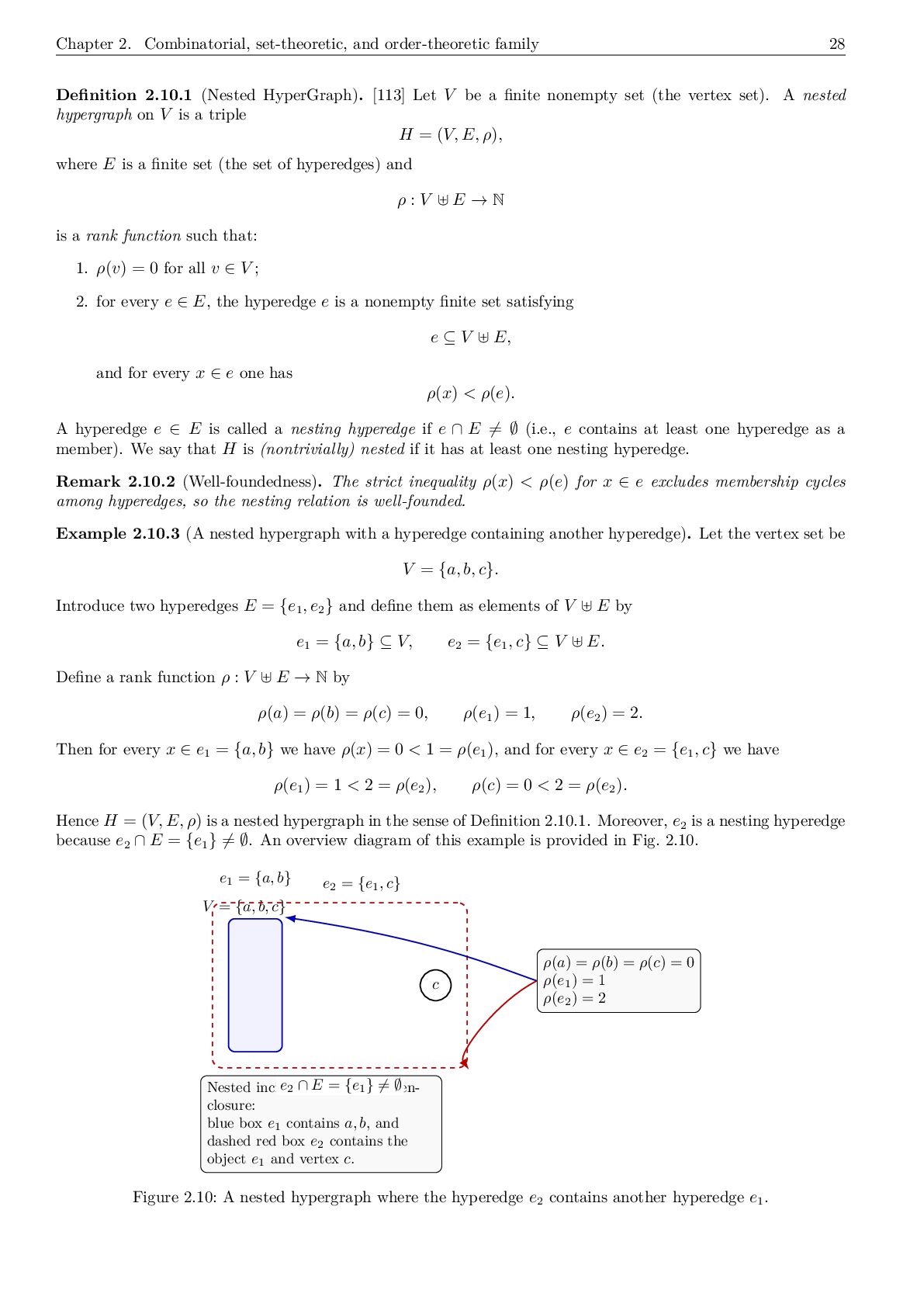
  28. Chapter 2. Combinatorial, set-theoretic, and order-theoretic family 28 Definition 2.10.1

    (Nested HyperGraph). [113] Let V be a finite nonempty set (the vertex set). A nested hypergraph on V is a triple H = (V, E, ρ), where E is a finite set (the set of hyperedges) and ρ : V E → N is a rank function such that: 1. ρ(v) = 0 for all v ∈ V ; 2. for every e ∈ E, the hyperedge e is a nonempty finite set satisfying e ⊆ V E, and for every x ∈ e one has ρ(x) < ρ(e). A hyperedge e ∈ E is called a nesting hyperedge if e ∩ E = ∅ (i.e., e contains at least one hyperedge as a member). We say that H is (nontrivially) nested if it has at least one nesting hyperedge. Remark 2.10.2 (Well-foundedness). The strict inequality ρ(x) < ρ(e) for x ∈ e excludes membership cycles among hyperedges, so the nesting relation is well-founded. Example 2.10.3 (A nested hypergraph with a hyperedge containing another hyperedge). Let the vertex set be V = {a, b, c}. Introduce two hyperedges E = {e1 , e2 } and define them as elements of V E by e1 = {a, b} ⊆ V, e2 = {e1 , c} ⊆ V E. Define a rank function ρ : V E → N by ρ(a) = ρ(b) = ρ(c) = 0, ρ(e1 ) = 1, ρ(e2 ) = 2. Then for every x ∈ e1 = {a, b} we have ρ(x) = 0 < 1 = ρ(e1 ), and for every x ∈ e2 = {e1 , c} we have ρ(e1 ) = 1 < 2 = ρ(e2 ), ρ(c) = 0 < 2 = ρ(e2 ). Hence H = (V, E, ρ) is a nested hypergraph in the sense of Definition 2.10.1. Moreover, e2 is a nesting hyperedge because e2 ∩ E = {e1 } = ∅. An overview diagram of this example is provided in Fig. 2.10. a b c V = {a, b, c} e1 = {a, b} e2 = {e1 , c} ρ(a) = ρ(b) = ρ(c) = 0 ρ(e1 ) = 1 ρ(e2 ) = 2 Nested incidence is shown by en- closure: blue box e1 contains a, b, and dashed red box e2 contains the object e1 and vertex c. e2 ∩ E = {e1 } = ∅ Figure 2.10: A nested hypergraph where the hyperedge e2 contains another hyperedge e1 .
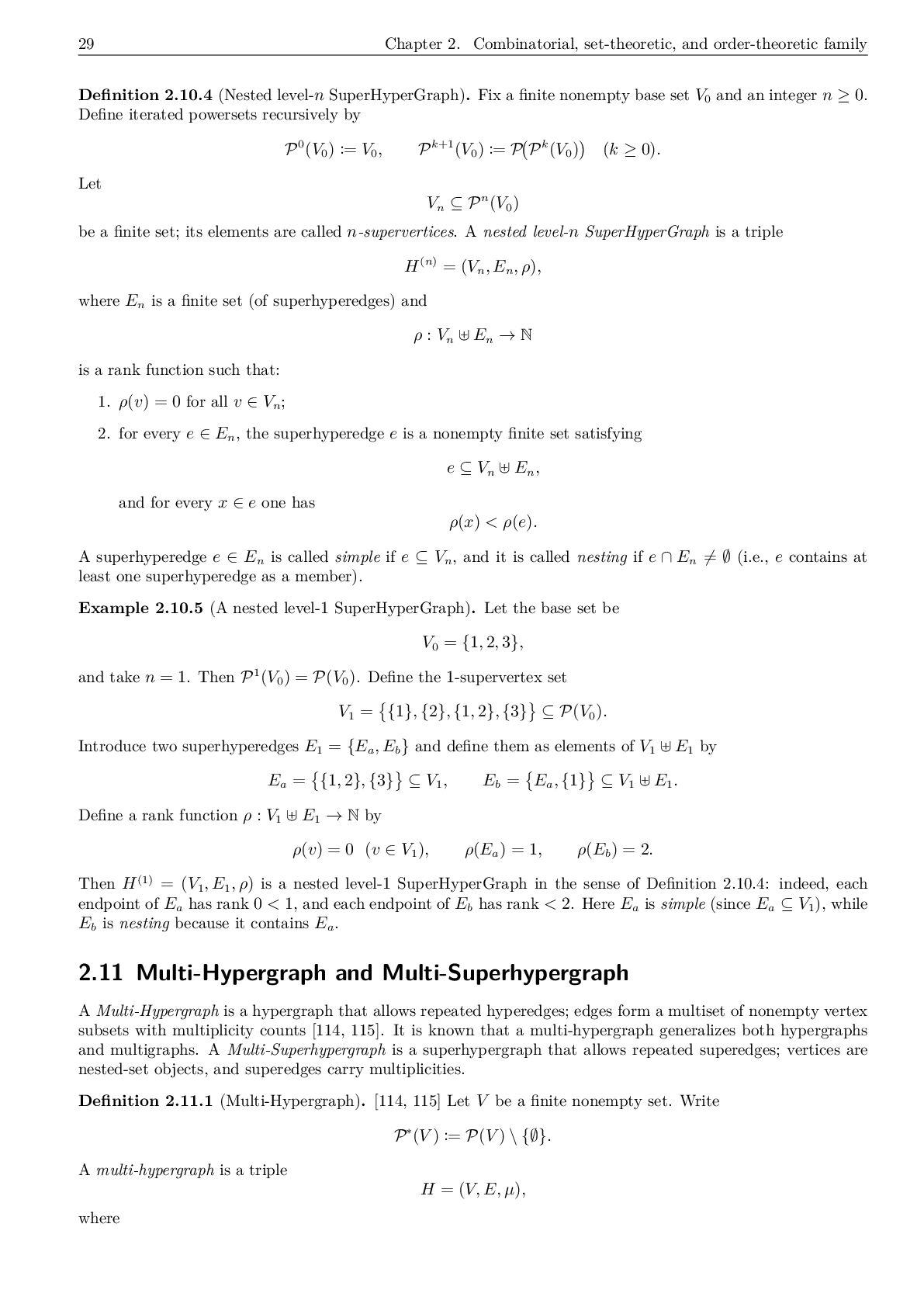
  29. 29 Chapter 2. Combinatorial, set-theoretic, and order-theoretic family Definition 2.10.4

    (Nested level-n SuperHyperGraph). Fix a finite nonempty base set V0 and an integer n ≥ 0. Define iterated powersets recursively by P0(V0 ) := V0 , Pk+1(V0 ) := P Pk(V0 ) (k ≥ 0). Let Vn ⊆ Pn(V0 ) be a finite set; its elements are called n-supervertices. A nested level-n SuperHyperGraph is a triple H(n) = (Vn , En , ρ), where En is a finite set (of superhyperedges) and ρ : Vn En → N is a rank function such that: 1. ρ(v) = 0 for all v ∈ Vn ; 2. for every e ∈ En , the superhyperedge e is a nonempty finite set satisfying e ⊆ Vn En , and for every x ∈ e one has ρ(x) < ρ(e). A superhyperedge e ∈ En is called simple if e ⊆ Vn , and it is called nesting if e ∩ En = ∅ (i.e., e contains at least one superhyperedge as a member). Example 2.10.5 (A nested level-1 SuperHyperGraph). Let the base set be V0 = {1, 2, 3}, and take n = 1. Then P1(V0 ) = P(V0 ). Define the 1-supervertex set V1 = {1}, {2}, {1, 2}, {3} ⊆ P(V0 ). Introduce two superhyperedges E1 = {Ea , Eb } and define them as elements of V1 E1 by Ea = {1, 2}, {3} ⊆ V1 , Eb = Ea , {1} ⊆ V1 E1 . Define a rank function ρ : V1 E1 → N by ρ(v) = 0 (v ∈ V1 ), ρ(Ea ) = 1, ρ(Eb ) = 2. Then H(1) = (V1 , E1 , ρ) is a nested level-1 SuperHyperGraph in the sense of Definition 2.10.4: indeed, each endpoint of Ea has rank 0 < 1, and each endpoint of Eb has rank < 2. Here Ea is simple (since Ea ⊆ V1 ), while Eb is nesting because it contains Ea . 2.11 Multi-Hypergraph and Multi-Superhypergraph A Multi-Hypergraph is a hypergraph that allows repeated hyperedges; edges form a multiset of nonempty vertex subsets with multiplicity counts [114, 115]. It is known that a multi-hypergraph generalizes both hypergraphs and multigraphs. A Multi-Superhypergraph is a superhypergraph that allows repeated superedges; vertices are nested-set objects, and superedges carry multiplicities. Definition 2.11.1 (Multi-Hypergraph). [114, 115] Let V be a finite nonempty set. Write P∗(V ) := P(V ) \ {∅}. A multi-hypergraph is a triple H = (V, E, µ), where
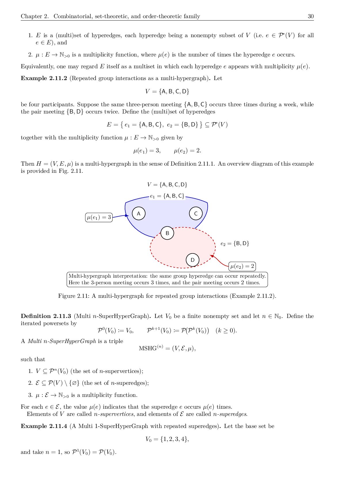
  30. Chapter 2. Combinatorial, set-theoretic, and order-theoretic family 30 1. E

    is a (multi)set of hyperedges, each hyperedge being a nonempty subset of V (i.e. e ∈ P∗(V ) for all e ∈ E), and 2. µ : E → N>0 is a multiplicity function, where µ(e) is the number of times the hyperedge e occurs. Equivalently, one may regard E itself as a multiset in which each hyperedge e appears with multiplicity µ(e). Example 2.11.2 (Repeated group interactions as a multi-hypergraph). Let V = {A, B, C, D} be four participants. Suppose the same three-person meeting {A, B, C} occurs three times during a week, while the pair meeting {B, D} occurs twice. Define the (multi)set of hyperedges E = e1 = {A, B, C}, e2 = {B, D} ⊆ P∗(V ) together with the multiplicity function µ : E → N>0 given by µ(e1 ) = 3, µ(e2 ) = 2. Then H = (V, E, µ) is a multi-hypergraph in the sense of Definition 2.11.1. An overview diagram of this example is provided in Fig. 2.11. V = {A, B, C, D} A B C D e1 = {A, B, C} e2 = {B, D} µ(e1 ) = 3 µ(e2 ) = 2 Multi-hypergraph interpretation: the same group hyperedge can occur repeatedly. Here the 3-person meeting occurs 3 times, and the pair meeting occurs 2 times. Figure 2.11: A multi-hypergraph for repeated group interactions (Example 2.11.2). Definition 2.11.3 (Multi n-SuperHyperGraph). Let V0 be a finite nonempty set and let n ∈ N0 . Define the iterated powersets by P0(V0 ) := V0 , Pk+1(V0 ) := P Pk(V0 ) (k ≥ 0). A Multi n-SuperHyperGraph is a triple MSHG(n) = (V, E, µ), such that 1. V ⊆ Pn(V0 ) (the set of n-supervertices); 2. E ⊆ P(V ) \ {∅} (the set of n-superedges); 3. µ : E → N>0 is a multiplicity function. For each e ∈ E, the value µ(e) indicates that the superedge e occurs µ(e) times. Elements of V are called n-supervertices, and elements of E are called n-superedges. Example 2.11.4 (A Multi 1-SuperHyperGraph with repeated superedges). Let the base set be V0 = {1, 2, 3, 4}, and take n = 1, so P1(V0 ) = P(V0 ).
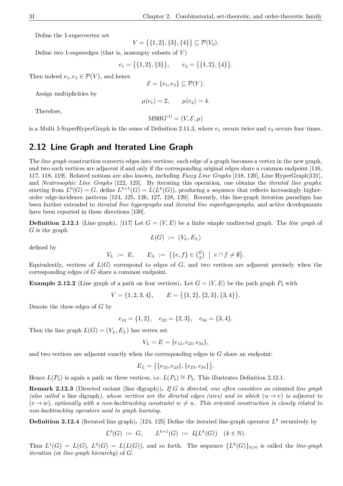
  31. 31 Chapter 2. Combinatorial, set-theoretic, and order-theoretic family Define the

    1-supervertex set V = {1, 2}, {3}, {4} ⊆ P(V0 ). Define two 1-superedges (that is, nonempty subsets of V ) e1 = {1, 2}, {3} , e2 = {1, 2}, {4} . Then indeed e1 , e2 ∈ P(V ), and hence E = {e1 , e2 } ⊆ P(V ). Assign multiplicities by µ(e1 ) = 2, µ(e2 ) = 4. Therefore, MSHG(1) = (V, E, µ) is a Multi 1-SuperHyperGraph in the sense of Definition 2.11.3, where e1 occurs twice and e2 occurs four times. 2.12 Line Graph and Iterated Line Graph The line graph construction converts edges into vertices: each edge of a graph becomes a vertex in the new graph, and two such vertices are adjacent if and only if the corresponding original edges share a common endpoint [116, 117, 118, 119]. Related notions are also known, including Fuzzy Line Graphs [118, 120], Line HyperGraph[121], and Neutrosophic Line Graphs [122, 123]. By iterating this operation, one obtains the iterated line graphs: starting from L0(G) = G, define Lk+1(G) = L(Lk(G)), producing a sequence that reflects increasingly higher- order edge-incidence patterns [124, 125, 126, 127, 128, 129]. Recently, this line-graph iteration paradigm has been further extended to iterated line hypergraphs and iterated line superhypergraphs, and active developments have been reported in these directions [130]. Definition 2.12.1 (Line graph). [117] Let G = (V, E) be a finite simple undirected graph. The line graph of G is the graph L(G) := (VL , EL ) defined by VL := E, EL := {e, f} ∈ E 2 e ∩ f = ∅ . Equivalently, vertices of L(G) correspond to edges of G, and two vertices are adjacent precisely when the corresponding edges of G share a common endpoint. Example 2.12.2 (Line graph of a path on four vertices). Let G = (V, E) be the path graph P4 with V = {1, 2, 3, 4}, E = {1, 2}, {2, 3}, {3, 4} . Denote the three edges of G by e12 = {1, 2}, e23 = {2, 3}, e34 = {3, 4}. Then the line graph L(G) = (VL , EL ) has vertex set VL = E = {e12 , e23 , e34 }, and two vertices are adjacent exactly when the corresponding edges in G share an endpoint: EL = {e12 , e23 }, {e23 , e34 } . Hence L(P4 ) is again a path on three vertices, i.e. L(P4 ) ∼ = P3 . This illustrates Definition 2.12.1. Remark 2.12.3 (Directed variant (line digraph)). If G is directed, one often considers an oriented line graph (also called a line digraph), whose vertices are the directed edges (arcs) and in which (u → v) is adjacent to (v → w), optionally with a non-backtracking constraint w = u. This oriented construction is closely related to non-backtracking operators used in graph learning. Definition 2.12.4 (Iterated line graph). [124, 125] Define the iterated line-graph operator Lk recursively by L0(G) := G, Lk+1(G) := L Lk(G) (k ∈ N). Thus L1(G) = L(G), L2(G) = L(L(G)), and so forth. The sequence {Lk(G)}k≥0 is called the line-graph iteration (or line-graph hierarchy) of G.
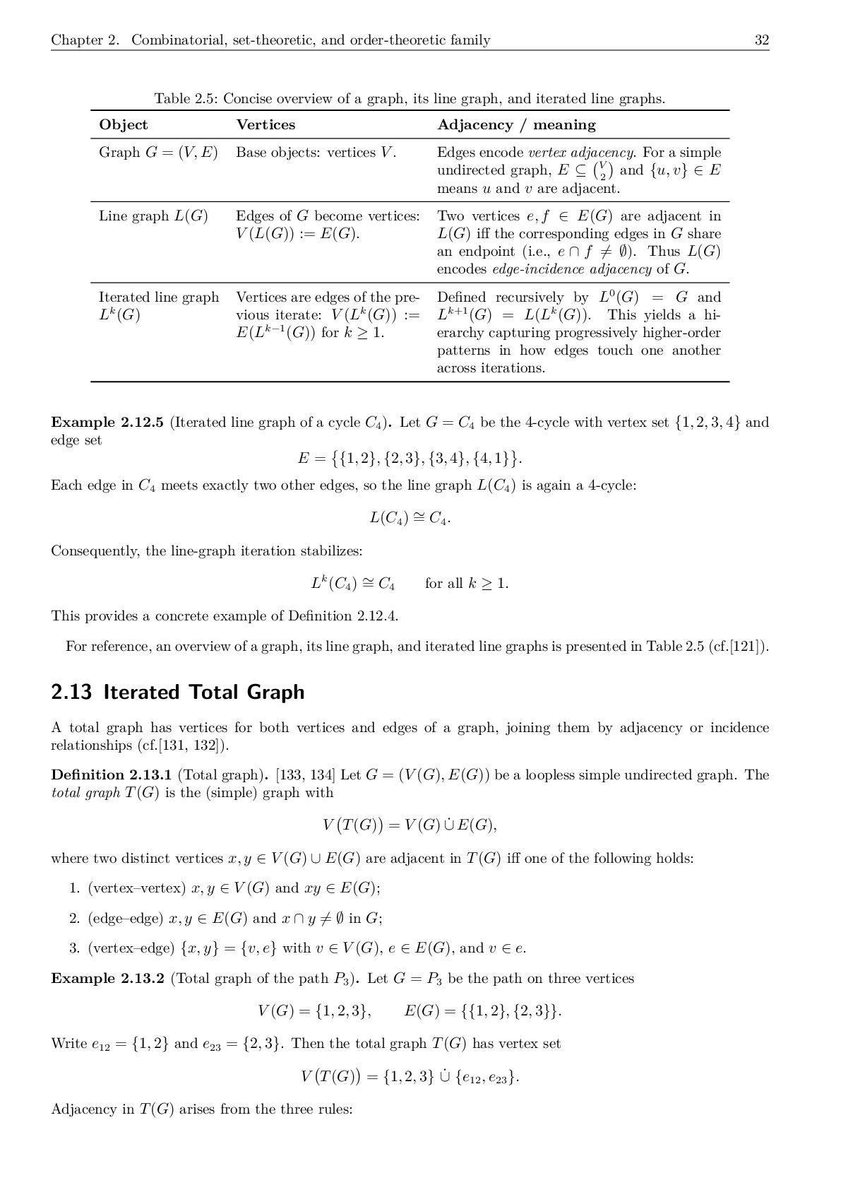
  32. Chapter 2. Combinatorial, set-theoretic, and order-theoretic family 32 Table 2.5:

    Concise overview of a graph, its line graph, and iterated line graphs. Object Vertices Adjacency / meaning Graph G = (V, E) Base objects: vertices V . Edges encode vertex adjacency. For a simple undirected graph, E ⊆ V 2 and {u, v} ∈ E means u and v are adjacent. Line graph L(G) Edges of G become vertices: V (L(G)) := E(G). Two vertices e, f ∈ E(G) are adjacent in L(G) iff the corresponding edges in G share an endpoint (i.e., e ∩ f = ∅). Thus L(G) encodes edge-incidence adjacency of G. Iterated line graph Lk(G) Vertices are edges of the pre- vious iterate: V (Lk(G)) := E(Lk−1(G)) for k ≥ 1. Defined recursively by L0(G) = G and Lk+1(G) = L(Lk(G)). This yields a hi- erarchy capturing progressively higher-order patterns in how edges touch one another across iterations. Example 2.12.5 (Iterated line graph of a cycle C4 ). Let G = C4 be the 4-cycle with vertex set {1, 2, 3, 4} and edge set E = {1, 2}, {2, 3}, {3, 4}, {4, 1} . Each edge in C4 meets exactly two other edges, so the line graph L(C4 ) is again a 4-cycle: L(C4 ) ∼ = C4 . Consequently, the line-graph iteration stabilizes: Lk(C4 ) ∼ = C4 for all k ≥ 1. This provides a concrete example of Definition 2.12.4. For reference, an overview of a graph, its line graph, and iterated line graphs is presented in Table 2.5 (cf.[121]). 2.13 Iterated Total Graph A total graph has vertices for both vertices and edges of a graph, joining them by adjacency or incidence relationships (cf.[131, 132]). Definition 2.13.1 (Total graph). [133, 134] Let G = (V (G), E(G)) be a loopless simple undirected graph. The total graph T(G) is the (simple) graph with V T(G) = V (G) ˙ ∪ E(G), where two distinct vertices x, y ∈ V (G) ∪ E(G) are adjacent in T(G) iff one of the following holds: 1. (vertex–vertex) x, y ∈ V (G) and xy ∈ E(G); 2. (edge–edge) x, y ∈ E(G) and x ∩ y = ∅ in G; 3. (vertex–edge) {x, y} = {v, e} with v ∈ V (G), e ∈ E(G), and v ∈ e. Example 2.13.2 (Total graph of the path P3 ). Let G = P3 be the path on three vertices V (G) = {1, 2, 3}, E(G) = {{1, 2}, {2, 3}}. Write e12 = {1, 2} and e23 = {2, 3}. Then the total graph T(G) has vertex set V T(G) = {1, 2, 3} ˙ ∪ {e12 , e23 }. Adjacency in T(G) arises from the three rules:
  33. 33 Chapter 2. Combinatorial, set-theoretic, and order-theoretic family • vertex–vertex:

    1 ∼ 2 and 2 ∼ 3 (since {1, 2}, {2, 3} ∈ E(G)); • edge–edge: e12 ∼ e23 (since e12 ∩ e23 = {2} = ∅ in G); • vertex–edge: 1 ∼ e12 , 2 ∼ e12 , 2 ∼ e23 , 3 ∼ e23 (because each vertex is adjacent to its incident edges). Thus T(P3 ) is a simple graph on five vertices encoding both adjacency and incidence information of P3 , as in the definition of the total graph. An iterated total graph repeatedly applies the total graph operation to a graph, incorporating vertices, edges, and all incidence relationships at each stage [132, 131]. Definition 2.13.3 (Iterated total graphs). Define T0(G) := G, and for each integer k ≥ 1 set Tk(G) := T T k−1(G) . (Thus T1(G) = T(G), T2(G) = T(T(G)), etc.) This notation is also used in the literature. Example 2.13.4 (Iterated total graphs starting from K2 ). Let G = K2 be the complete graph on two vertices: V (G) = {1, 2}, E(G) = {{1, 2}}. Let e = {1, 2} denote the unique edge. Then the total graph T(G) has vertex set V T(G) = {1, 2, e} and edges {1, 2}, {1, e}, {2, e}, so T(K2 ) ∼ = K3 . Applying the total operation again yields T2(K2 ) = T T(K2 ) = T(K3 ). Since K3 has three vertices and three edges, T(K3 ) has 6 vertices and encodes all vertex–vertex, edge–edge, and vertex–edge incidences of K3 . Hence (Tk(K2 ))k≥0 provides a concrete iterated total-graph hierarchy K2 = T0(K2 ) −→ T1(K2 ) ∼ = K3 −→ T2(K2 ) = T(K3 ) −→ · · · , illustrating the definition of iterated total graphs. 2.14 Hierarchical SuperHyperGraph A hierarchical superhypergraph is a superhypergraph whose vertices live across multiple powerset levels, with edges allowed to join mixed-level supervertices, while maintaining downward-closure coherence (cf.[135, 136]). Definition 2.14.1 (Support map and edge-support). Define the support map supp : V → P(V0 )\{∅} recursively by supp(v) := {v} (v ∈ V0 ), supp(X) := y∈X supp(y) (X ∈ V \ V0 ), and for each e ∈ E define its base support (a hyperedge on V0 ) by σ(e) := x∈e supp(x) ∈ P(V0 ) \ {∅}. Definition 2.14.2 (Hierarchical SuperHyperGraph of height r). (cf.[135, 136]) Let V0 be a finite, nonempty base set. For k ≥ 0 define iterated powersets P0(V0 ) := V0 , P k+1(V0 ) := P P k(V0 ) , and fix an integer r ≥ 0. Set the hierarchical universe Ur (V0 ) := r k=0 P k(V0 ) \ {∅} .
  34. Chapter 2. Combinatorial, set-theoretic, and order-theoretic family 34 For x

    ∈ Ur (V0 ), define its level (x) := min{ k ∈ {0, 1, . . . , r} : x ∈ P k(V0 ) }. A hierarchical superhypergraph of height r on V0 is a pair H r = (V, E) such that (H1) (Hierarchical vertex set) V is a finite nonempty set with V ⊆ Ur (V0 ). Elements of V are called hierarchical supervertices. (H2) (Cross-level edges) E is a finite family of nonempty subsets of V : E ⊆ P(V ) \ {∅}. Elements of E are called hierarchical superhyperedges. In particular, a superhyperedge may contain su- pervertices of different levels. (H3) (Coherence / downward closure) If X ∈ V and (X) ≥ 1, then X ⊆ V. Equivalently, whenever a higher-level supervertex is present, all its immediate constituents are also present as supervertices. For each k ∈ {0, . . . , r} we define the k-th layer by Vk := { x ∈ V : (x) = k }, so that V = ˙ r k=0 Vk . Example 2.14.3 (A hierarchical SuperHyperGraph of height 2 with cross-level edges). Let the base set be V0 = {a, b, c, d}. Consider the hierarchical universe U2 (V0 ) = V0 ∪ P(V0 ) \ {∅} ∪ P(P(V0 )) \ {∅} . Define hierarchical supervertices (across levels 0, 1, 2) by X = {a, b} ∈ P(V0 ), Y = {c, d} ∈ P(V0 ), U = {X} = {{a, b}} ∈ P(P(V0 )). Set V = {a, b, c, d, X, Y, U} ⊆ U2 (V0 ). This V satisfies the coherence condition (H3): since X, Y ∈ V (level 1), their elements a, b, c, d belong to V ; and since U ∈ V (level 2), its element X belongs to V . Next, define a family of hierarchical superhyperedges E = {e1 , e2 }, e1 = {X, Y }, e2 = {U, c}. Thus e1 links two level-1 supervertices (two teams), while e2 links a level-2 supervertex (a nested unit) to a level-0 vertex (an individual), illustrating a cross-level edge as allowed by (H2). Therefore H 2 = (V, E) is a hierarchical superhypergraph of height 2 in the sense of Definition 2.14.2. Support map and edge-support. Using Definition 2.14.1, the support map Supp satisfies Supp(a) = {a}, Supp(b) = {b}, Supp(c) = {c}, Supp(d) = {d}, Supp(X) = Supp({a, b}) = {a, b}, Supp(Y ) = {c, d}, Supp(U) = Supp({X}) = Supp(X) = {a, b}. Hence the base supports of the two edges are σ(e1 ) = Supp(X) ∪ Supp(Y ) = {a, b, c, d}, σ(e2 ) = Supp(U) ∪ Supp(c) = {a, b, c}. An overview diagram of this example is provided in Fig. 2.12.
  35. 35 Chapter 2. Combinatorial, set-theoretic, and order-theoretic family Level 2

    Level 1 Level 0 U = {{a, b}} X = {a, b} Y = {c, d} a b c d e1 e2 σ(e1 ) = {a, b, c, d} σ(e2 ) = {a, b, c} Figure 2.12: A hierarchical superhypergraph of height 2: vertices may live on different levels and edges may cross levels. Dashed lines indicate constituent relations (coherence), while e1 , e2 are superhyperedges. 2.15 Recursive HyperGraph and Recursive SuperHyperGraph A recursive hypergraph is a hypergraph-like object in which a hyperedge may contain ordinary vertices and also lower-level hyperedges as elements, thereby permitting nested incidence up to a prescribed recursion depth [137, 138, 139, 140]. Definition 2.15.1 (Depth-k powerset universe). [137, 140] Let S be a nonempty set and let k ∈ N∪{0}. Define a hierarchy of sets (Si )i≥0 by S0 := S, Si := P i−1 j=0 Sj (i ≥ 1). Set US,k := k i=0 Si . The depth-k powerset universe over S is 2S,k := P(US,k ). Definition 2.15.2 (k-recursive hypergraph). [137, 140] Let V be a finite vertex set and let k ∈ N ∪ {0}. A k-recursive hypergraph is a pair H = (V, E) such that E ⊆ 2V,k \ {∅}, where 2V,k is the depth-k powerset universe from Definition 2.15.1 applied to S = V . In particular, for k = 0 one has 2V,0 = P(V ) and thus E ⊆ P(V ) \ {∅}, i.e., H reduces to an ordinary hypergraph. Example 2.15.3 (A 1-recursive hypergraph (edge-of-edges for task bundles)). Let V = {a, b, c, d} be four tasks. Consider two ordinary hyperedges (task bundles) e1 = {a, b}, e2 = {c, d}. A 1-recursive hyperedge may contain vertices and also lower-level hyperedges as elements. Define e3 = {e1 , c}, which represents a higher-level bundle “do the bundle {a, b} together with task c.” Let E = {e1 , e2 , e3 }. Then H = (V, E) is a 1-recursive hypergraph in the sense of Definition 2.15.2: indeed, e1 , e2 ∈ 2V,0 = P(V ) and e3 ∈ 2V,1 because it mixes a depth-0 hyperedge e1 with a vertex c. An overview diagram of this example is provided in Fig. 2.13. An (n, k)-recursive SuperHyperGraph combines hierarchical supervertices (via iterated powersets) with recur- sive superhyperedges of bounded depth k, allowing edges to contain supervertices and nested lower-level edges as elements.
  36. Chapter 2. Combinatorial, set-theoretic, and order-theoretic family 36 depth 1

    (recursive) depth 0 (hyperedges) vertices a b c d e1 = {a, b} e2 = {c, d} e3 = {e1 , c} V = {a, b, c, d} E = {e1 , e2 , e3 } Recursive incidence: e3 contains the hyperedge-object e1 and the vertex c. Figure 2.13: A schematic illustration of the 1-recursive hypergraph in Example 2.15.3. The recursive hyperedge e3 contains a lower-level hyperedge e1 and a vertex c. Definition 2.15.4 ((n, k)-recursive SuperHyperGraph). [141, 142, 143] Fix a finite nonempty base set V0 and let n, k ∈ N ∪ {0}. An (n, k)-recursive SuperHyperGraph is a pair RSHG(n,k) = (V, E) satisfying: (i) (Hierarchical supervertex set). V ⊆ P n(V0 ). (ii) (Recursive superhyperedge family). E ⊆ 2V,k \{∅}, where 2V,k is the depth-k powerset universe constructed from S = V as in Definition 2.15.1. Example 2.15.5 (A (1, 1)-recursive SuperHyperGraph (teams with a recursive superedge)). Let the base set be V0 = {1, 2, 3, 4}, and take n = 1, so P1(V0 ) = P(V0 ). Define the 1-supervertex set (teams) V = {1, 2}, {3}, {4} ⊆ P(V0 ). Consider two ordinary superhyperedges (depth 0 edges in P(V )): e1 = {1, 2}, {3} , e2 = {1, 2}, {4} . Now form a recursive superhyperedge of depth 1 by letting e3 = {e1 , {4}} ∈ 2V,1 , which can be read as a higher-level interaction “activate the collaboration e1 and also involve the team {4}.” Let E = {e1 , e2 , e3 } ⊆ 2V,1 \ {∅}. Then RSHG(1,1) = (V, E) is a (1, 1)-recursive SuperHyperGraph in the sense of Definition 2.15.4. 2.16 Tree-Vertex Graph A tree-vertex graph labels tree nodes by nested vertex-sets; edges connect nodes within levels, representing relations across abstraction depths [144]. Definition 2.16.1 (Depth-n Tree-Vertex Graph with level edges). [144] Let V0 be a finite, nonempty set of base vertices and let n ∈ N. A depth-n Tree-Vertex Graph (TVG) on V0 is a quadruple TVG(n) = V0 , T, η, {E(k)}n k=0 , where:
  37. 37 Chapter 2. Combinatorial, set-theoretic, and order-theoretic family (i) T

    = (N, F, r) is a rooted tree whose leaves have depth 0 and whose root has depth n. For each k ∈ {0, . . . , n} define the level set Nk := {u ∈ N | depth(u) = k}. (ii) η is a nested labeling (level-typed label map) η : N −→ n k=0 PSk(V0 ) \ {∅} satisfying: (a) (Level-typing) For every u ∈ Nk , one has η(u) ∈ PSk(V0 ) \ {∅}. (b) (Leaf grounding) The restriction η|N0 : N0 → V0 is a bijection (so each leaf represents exactly one base vertex). (c) (Recursive nesting along the tree) For every internal node u ∈ Nk with k ≥ 1, η(u) = {η(v) | v ∈ Ch(u)}, so the label of u is literally the set of its children’s labels (hence lives in the next iterated powerset). (iii) The support (flattened base-vertex set) of a tree-vertex u ∈ Nk is defined by λ(u) := Flat k (η(u)) ⊆ V0 . (iv) For each level k ∈ {0, . . . , n}, E(k) is a set of level-k graph edges: E(k) ⊆ {u, v} ⊆ Nk | u = v . An edge {u, v} ∈ E(k) encodes a binary relation within the same abstraction depth k between the hierar- chical units represented by u and v. Example 2.16.2 (A depth-2 Tree-Vertex Graph for a small organization). Let the base vertices be four em- ployees V0 = {a, b, c, d}. We construct a depth-2 Tree-Vertex Graph TVG(2) in the sense of Definition 2.16.1. (1) The rooted tree. Let T = (N, F, r) be the rooted tree with node set N = {r, u1 , u2 , a0 , b0 , c0 , d0 }, root r at depth 2, internal nodes u1 , u2 at depth 1, and leaves N0 = {a0 , b0 , c0 , d0 }, N1 = {u1 , u2 }, N2 = {r}. Define the parent–child relations by Ch(r) = {u1 , u2 }, Ch(u1 ) = {a0 , b0 }, Ch(u2 ) = {c0 , d0 }. Thus the tree groups employees into two teams {a, b} and {c, d}, and then into one department. (2) Nested labeling. Define η : N → 2 k=0 PSk(V0 ) \ {∅} by η(a0 ) = a, η(b0 ) = b, η(c0 ) = c, η(d0 ) = d, η(u1 ) = {η(a0 ), η(b0 )} = {a, b}, η(u2 ) = {η(c0 ), η(d0 )} = {c, d}, η(r) = {η(u1 ), η(u2 )} = {a, b}, {c, d} . By construction, η|N0 is a bijection onto V0 , and each internal label is exactly the set of its children’s labels.
  38. Chapter 2. Combinatorial, set-theoretic, and order-theoretic family 38 r u1

    u2 a0 b0 c0 d0 E(0) : {a0, b0} E(0) : {c0, d0} E(1) : {u1, u2} depth 2 depth 1 depth 0 η(a0) = a λ(a0) = {a} η(b0) = b λ(b0) = {b} η(c0) = c λ(c0) = {c} η(d0) = d λ(d0) = {d} η(u1) = {a, b} λ(u1) = {a, b} η(u2) = {c, d} λ(u2) = {c, d} η(r) = { {a, b}, {c, d} } λ(r) = {a, b, c, d} E(2) = ∅ Legend: Tree edges = parent–child links. Solid curved links indicate level-0 edges E(0) (employee-level communication). Dashed curved link indicates the level-1 edge E(1) (team-level coordination). Figure 2.14: A depth-2 Tree-Vertex Graph for a small organization (Example 2.16.2). Leaves represent employ- ees, internal nodes represent teams, and the root represents the department. (3) Supports. Let λ(u) = Flat k (η(u)) ⊆ V0 be the flattened support. Then λ(a0 ) = {a}, λ(b0 ) = {b}, λ(c0 ) = {c}, λ(d0 ) = {d}, λ(u1 ) = {a, b}, λ(u2 ) = {c, d}, λ(r) = {a, b, c, d}. (4) Level edges. Define level-k edge sets by E(0) = {a0 , b0 }, {c0 , d0 } , E(1) = {u1 , u2 } , E(2) = ∅. Here E(0) encodes pairwise communication links inside each team at the employee level, while E(1) encodes a coordination link between the two teams. Therefore, TVG(2) = V0 , T, η, {E(k)}2 k=0 is a depth-2 Tree-Vertex Graph on V0 . An overview diagram of this example is provided in Fig. 2.14. 2.17 Tensor network graph A tensor network graph assigns tensors to vertices and index bonds to edges; contracting edges sums shared in- dices, yielding a tensor [145, 146]. A tensor network graph encodes higher-order interactions as tensors on nodes, with edges denoting index contractions, representing multiway correlations compactly for efficient computation and inference. Definition 2.17.1 (Tensor network graph). A tensor network graph is a triple N = (G, (Tv )v∈V (G) , (Ie )e∈E(G) ),
  39. 39 Chapter 2. Combinatorial, set-theoretic, and order-theoretic family where G

    is a finite (multi)graph, each vertex v ∈ V (G) is assigned a tensor Tv ∈ e∈Inc(v) KIe over a field K (typically R or C), and each edge e ∈ E(G) is assigned a finite index set Ie (equivalently, a bond dimension |Ie |). Here Inc(v) denotes the multiset of edges incident to v; half-edges (dangling edges) represent open indices (external legs). The value (or contraction) of N is the tensor obtained by summing over all internal indices corresponding to non-dangling edges, i.e. contracting the paired index spaces KIe ⊗ KIe along each internal edge e. Example 2.17.2 (A tensor network graph for a length-3 matrix product state). Let K = R. Consider a path graph on three vertices G : v1 − v2 − v3 , with two internal edges e12 and e23 , and with one dangling half-edge attached to each vertex (representing a physical/open index). Assign index sets I12 = {1, . . . , D}, I23 = {1, . . . , D} to the internal edges (bond dimension D), and assign I1 = {1, . . . , d}, I2 = {1, . . . , d}, I3 = {1, . . . , d} to the three dangling edges (physical dimension d). Assign tensors Tv1 ∈ Rd×D, Tv2 ∈ RD×d×D, Tv3 ∈ RD×d so that Tv1 has indices (i1 , α), Tv2 has indices (α, i2 , β), and Tv3 has indices (β, i3 ) with ij ∈ {1, . . . , d} and α, β ∈ {1, . . . , D}. Then the tensor network contraction produces a 3-way tensor Ψ ∈ Rd×d×d whose entries are given by Ψi1i2i3 = D α=1 D β=1 Tv1 i1,α Tv2 α,i2,β Tv3 β,i3 . Thus N = (G, (Tv )v∈V (G) , (Ie )e∈E(G) ) is a tensor network graph in the sense of Definition 2.17.1; the internal edges e12 , e23 are contracted (summed over), while the three dangling edges remain as open indices. 2.18 MultiTensor and Iterated MultiTensor Network MultiTensor Network assigns each node a finite multiset of compatible local tensors, generating multiple weighted contractions through realization choices while preserving one external tensor space. Iterated MultiTensor Net- work assigns nodes iterated finite multisets of compatible local tensors, recursively flattening multiplicities into effective multitensor assignments before canonically computing weighted network contractions. Definition 2.18.1 (Finite multiset). Let X be a set. A finite multiset on X is a function m : X → N0 with finite support supp(m) := {x ∈ X : m(x) > 0}. We write Mfin(X) for the set of all finite multisets on X. If x ∈ X, then m(x) is called the multiplicity of x in m.
  40. Chapter 2. Combinatorial, set-theoretic, and order-theoretic family 40 Definition 2.18.2

    (MultiTensor network graph). Let Tv := e∈Inc(v) KIe denote the local tensor space associated with a vertex v of a finite graph G, where K is a field and each edge or half-edge e is assigned a finite index set Ie . A MultiTensor network graph is a triple Nmulti = G, (Mv )v∈V (G) , (Ie )e∈E(G) , such that: • G is a finite (multi)graph, possibly with dangling half-edges; • for each edge e, Ie is a finite index set; • for each vertex v ∈ V (G), Mv ∈ Mfin(Tv ) is a finite multiset of tensors of the same local type Tv . A realization of Nmulti is a choice τ = (Tv )v∈V (G) such that Tv ∈ supp(Mv ) (∀ v ∈ V (G)). Its multiplicity is defined by µ(τ) := v∈V (G) Mv (Tv ). For each realization τ, its contraction Contr(τ) is the tensor obtained by contracting the ordinary tensor network graph G, (Tv )v∈V (G) , (Ie )e∈E(G) in the sense of Definition 2.17.1. The contraction multiset of Nmulti is the finite multiset of output tensors defined by Contrmulti Nmulti (X) := τ realization Contr(τ)=X µ(τ), for each output tensor X in the external tensor space determined by the dangling half-edges. If desired, one may also define the aggregated contraction by AContr Nmulti := τ realization µ(τ) Contr(τ), provided all output tensors belong to the same external tensor space. Definition 2.18.3 (Iterated finite multiset). For a set X, define recursively M0 fin (X) := X, Mn+1 fin (X) := Mfin Mn fin (X) (n ≥ 0). Thus, an element of Mn fin (X) is an n-fold iterated finite multiset over X. Example 2.18.4 (A concrete MultiTensor network graph). Let K = R, and let G be the graph with two vertices V (G) = {v1 , v2 } and one internal edge E(G) = {e}, e = {v1 , v2 }.
  41. 41 Chapter 2. Combinatorial, set-theoretic, and order-theoretic family Assign the

    index set Ie = {1, 2}. Since the only incident edge at each vertex is e, the local tensor spaces are Tv1 = RIe , Tv2 = RIe . Thus each local tensor may be identified with a vector in R2. Define A1 = (1, 0), A2 = (0, 1) ∈ R2, and B1 = (1, 1), B2 = (1, −1) ∈ R2. Now assign finite multisets of local tensors by Mv1 = 2[A1 ] + 1[A2 ], Mv2 = 1[B1 ] + 3[B2 ]. Equivalently, Mv1 (A1 ) = 2, Mv1 (A2 ) = 1, Mv2 (B1 ) = 1, Mv2 (B2 ) = 3, and all other multiplicities are zero. Hence Nmulti = G, (Mv )v∈V (G) , (Ie )e∈E(G) is a MultiTensor network graph. A realization of Nmulti is a choice τ = (Tv1 , Tv2 ) with Tv1 ∈ {A1 , A2 }, Tv2 ∈ {B1 , B2 }. Thus there are exactly four realizations: τ1 = (A1 , B1 ), τ2 = (A1 , B2 ), τ3 = (A2 , B1 ), τ4 = (A2 , B2 ). Since the network has no dangling half-edges, each contraction is a scalar. More precisely, Contr(τ) = i∈Ie Tv1 (i) Tv2 (i), which is just the standard dot product in R2. We compute: Contr(τ1 ) = A1 · B1 = (1, 0) · (1, 1) = 1, Contr(τ2 ) = A1 · B2 = (1, 0) · (1, −1) = 1, Contr(τ3 ) = A2 · B1 = (0, 1) · (1, 1) = 1, Contr(τ4 ) = A2 · B2 = (0, 1) · (1, −1) = −1. Their multiplicities are µ(τ1 ) = Mv1 (A1 )Mv2 (B1 ) = 2 · 1 = 2, µ(τ2 ) = Mv1 (A1 )Mv2 (B2 ) = 2 · 3 = 6, µ(τ3 ) = Mv1 (A2 )Mv2 (B1 ) = 1 · 1 = 1, µ(τ4 ) = Mv1 (A2 )Mv2 (B2 ) = 1 · 3 = 3. Therefore the contraction multiset is Contrmulti Nmulti = 9[1] + 3[−1], because the scalar value 1 occurs with total multiplicity 2 + 6 + 1 = 9,
  42. Chapter 2. Combinatorial, set-theoretic, and order-theoretic family 42 whereas the

    scalar value −1 occurs with multiplicity 3. The aggregated contraction is AContr Nmulti = 4 k=1 µ(τk ) Contr(τk ) = 2 · 1 + 6 · 1 + 1 · 1 + 3 · (−1) = 6. Thus this example explicitly illustrates how a MultiTensor network graph produces a finite multiset of con- traction values, together with an aggregated contraction. Moreover, each local multiset Mvi ∈ Mfin(Tvi ) = M1 fin (Tvi ), so this example is also the first-level case of the iterated finite multiset formalism. Definition 2.18.5 (Flattening of iterated multisets). Let X be a set. For each n ≥ 0, define recursively a map Flat n : Mn fin (X) → Mfin(X) as follows: • for n = 0, set Flat 0 (x) := δx (x ∈ X), where δx denotes the singleton multiset supported at x with multiplicity 1; • for n ≥ 0 and M ∈ Mn+1 fin (X), define Flat n+1 (M)(x) := A∈supp(M) M(A) Flat n (A)(x) (x ∈ X). Hence Flat n converts an iterated multiset into an ordinary finite multiset on X by recursively collecting multi- plicities. Definition 2.18.6 (n-Iterated MultiTensor network graph). Let n ≥ 0. For each vertex v ∈ V (G), let Tv := e∈Inc(v) KIe be the corresponding local tensor space. An n-Iterated MultiTensor network graph is a triple N(n) = G, (Θv )v∈V (G) , (Ie )e∈E(G) , such that: • G is a finite (multi)graph, possibly with dangling half-edges; • for each edge e, Ie is a finite index set; • for each vertex v ∈ V (G), Θv ∈ Mn fin (Tv ). Its effective local multiset at v is defined by Meff v := Flat n (Θv ) ∈ Mfin(Tv ). The effective MultiTensor network graph associated with N(n) is Neff := G, (Meff v )v∈V (G) , (Ie )e∈E(G) . The contraction multiset of N(n) is then defined by Contriter N(n) := Contrmulti Neff , and, whenever meaningful, its aggregated contraction is defined by AContr N(n) := AContr Neff . In particular: n = 0 =⇒ N(0) is an ordinary tensor network graph, and n = 1 =⇒ N(1) is exactly a MultiTensor network graph.
  43. 43 Chapter 2. Combinatorial, set-theoretic, and order-theoretic family Theorem 2.18.7

    (Well-definedness of MultiTensor network graph). Let Nmulti = G, (Mv )v∈V (G) , (Ie )e∈E(G) be a MultiTensor network graph in the sense of Definition 2.18.2. Then: 1. the set of realizations of Nmulti is finite; 2. for every realization τ = (Tv )v∈V (G) with Tv ∈ supp(Mv ), the ordinary tensor network contraction Contr(τ) is well-defined; 3. the contraction multiset Contrmulti Nmulti is well-defined; 4. the aggregated contraction AContr Nmulti = τ µ(τ) Contr(τ) is well-defined. Proof. For each vertex v ∈ V (G), the multiset Mv has finite support by definition, and V (G) is finite. Hence the set of realizations v∈V (G) supp(Mv ) is finite. Moreover, every tensor chosen at v lies in the same local tensor space Tv = e∈Inc(v) KIe , so any realization τ determines an ordinary tensor network graph with the same underlying graph G and the same index sets (Ie )e∈E(G) . Therefore its contraction Contr(τ) is well-defined in the sense of Definition 2.17.1. Since the external tensor space is determined only by the dangling half-edges of G and the index sets Ie , all tensors Contr(τ) belong to one and the same output space. Because there are only finitely many realizations and each multiplicity µ(τ) = v∈V (G) Mv (Tv ) is a well-defined nonnegative integer, both Contrmulti Nmulti and AContr Nmulti are well-defined. Theorem 2.18.8 (Well-definedness of Iterated MultiTensor network graph). Let N(n) = G, (Θv )v∈V (G) , (Ie )e∈E(G) be an n-Iterated MultiTensor network graph in the sense of Definition 2.18.6. Then: 1. for each vertex v ∈ V (G)), the flattening Flat n (Θv ) ∈ Mfin(Tv ) is well-defined;
  44. Chapter 2. Combinatorial, set-theoretic, and order-theoretic family 44 2. the

    effective network Neff = G, (Flat n (Θv ))v∈V (G) , (Ie )e∈E(G) is a well-defined MultiTensor network graph; 3. consequently, both Contriter N(n) and AContr N(n) are well-defined. Proof. We first show that Flat n is well-defined for every n ≥ 0 by induction on n. For n = 0, the map Flat 0 (x) = δx is well-defined. Assume that Flat n is well-defined. Let M ∈ Mn+1 fin (X). Since M has finite support and each Flat n (A) is a finite multiset on X, the formula Flat n+1 (M)(x) = A∈supp(M) M(A) Flat n (A)(x) defines a finite-support function X → N0 . Hence Flat n+1 (M) ∈ Mfin(X) is well-defined. Applying this with X = Tv for each vertex v, we obtain Flat n (Θv ) ∈ Mfin(Tv ), so the effective network Neff is a MultiTensor network graph. Therefore Theorem 2.18.7 applies, and the contraction multiset and aggregated contraction of Neff are well-defined. By definition, Contriter N(n) = Contrmulti Neff , AContr N(n) = AContr Neff , hence both are well-defined. 2.19 Tensor Hypernetwork and Tensor Superhypernetwork A Tensor Hypernetwork is a hypergraph-based tensor network where each vertex carries a tensor and each hyperedge links multiple tensors through shared index contractions simultaneously. A Tensor Superhypernet- work generalizes a tensor hypernetwork by replacing vertices with hierarchical supervertices, enabling tensor contractions over nested, multi-level, higher-order relational structures and systems formally. Definition 2.19.1 (Tensor Hypernetwork). Let H = (V, E) be a finite hypergraph, where E ⊆ P(V ) \ {∅}. For each hyperedge e ∈ E, fix a positive integer de , and write [de ] := {1, 2, . . . , de }. For each vertex v ∈ V , define its incident-edge set by I(v) := { e ∈ E | v ∈ e }. A tensor hypernetwork over a field K on H is a tuple N = H, (de )e∈E , (Tv )v∈V , where each local tensor is a function Tv : e∈I(v) [de ] → K. If I(v) = ∅, the empty product is interpreted as a singleton, so Tv ∈ K. The associated closed contraction (network value) is Z(N) := (ae)e∈E ∈ ∏ e∈E [de] v∈V Tv (ae )e∈I(v) ∈ K.
  45. 45 Chapter 2. Combinatorial, set-theoretic, and order-theoretic family Definition 2.19.2

    (Tensor n-SuperHyperNetwork). Let V0 be a finite nonempty base set, and define iterated powersets by P0(V0 ) := V0 , Pk+1(V0 ) := P Pk(V0 ) (k ≥ 0). Let SHG(n) = (V, E) be an n-SuperHyperGraph on V0 , that is, V ⊆ Pn(V0 ), E ⊆ P(V ) \ {∅}. Elements of V are called n-supervertices, and elements of E are called n-superedges. For each superedge e ∈ E, fix a positive integer de , and write [de ] := {1, 2, . . . , de }. For each supervertex x ∈ V , define I(x) := { e ∈ E | x ∈ e }. A tensor n-SuperHyperNetwork over a field K is a tuple N(n) = V0 ; V, E, (de )e∈E , (Tx )x∈V , where each local supertensor is a function Tx : e∈I(x) [de ] → K (x ∈ V ). If I(x) = ∅, the empty product is interpreted as a singleton, so Tx ∈ K. Its associated closed contraction is Z(N(n)) := (ae)e∈E ∈ ∏ e∈E [de] x∈V Tx (ae )e∈I(x) ∈ K. A tensor SuperHyperNetwork is a tensor n-SuperHyperNetwork for some n ≥ 1. Example 2.19.3 (A concrete tensor 1-SuperHyperNetwork). Let the base set be V0 = {a, b, c}. Since P1(V0 ) = P(V0 ), we may choose 1-supervertices as subsets of V0 . Define x1 := {a, b}, x2 := {b, c}, x3 := {a, c}, and set V = {x1 , x2 , x3 } ⊆ P(V0 ). Now define two 1-superedges by e1 := {x1 , x2 }, e2 := {x2 , x3 }. Thus E = {e1 , e2 } ⊆ P(V ) \ {∅}. Hence SHG(1) = (V, E) is a 1-SuperHyperGraph on V0 . Assign bond dimensions de1 = 2, de2 = 2, so that [de1 ] = [de2 ] = {1, 2}.
  46. Chapter 2. Combinatorial, set-theoretic, and order-theoretic family 46 For each

    supervertex, the incident superedge set is I(x1 ) = {e1 }, I(x2 ) = {e1 , e2 }, I(x3 ) = {e2 }. Let K = R. Define the local supertensors as follows: Tx1 : [2] → R, Tx1 (1) = 1, Tx1 (2) = 2, Tx2 : [2] × [2] → R, Tx2 (i, j) 2 i,j=1 = 1 0 3 1 , that is, Tx2 (1, 1) = 1, Tx2 (1, 2) = 0, Tx2 (2, 1) = 3, Tx2 (2, 2) = 1, and Tx3 : [2] → R, Tx3 (1) = 2, Tx3 (2) = 1. Therefore, N(1) = V0 ; V, E, (de )e∈E , (Tx )x∈V is a tensor 1-SuperHyperNetwork over R. Its closed contraction is Z(N(1)) = (ae1 ,ae2 )∈[2]×[2] Tx1 (ae1 ) Tx2 (ae1 , ae2 ) Tx3 (ae2 ). Writing i := ae1 and j := ae2 , we obtain Z(N(1)) = 2 i=1 2 j=1 Tx1 (i) Tx2 (i, j) Tx3 (j). Substituting the above values gives Z(N(1)) = Tx1 (1)Tx2 (1, 1)Tx3 (1) + Tx1 (1)Tx2 (1, 2)Tx3 (2) + Tx1 (2)Tx2 (2, 1)Tx3 (1) + Tx1 (2)Tx2 (2, 2)Tx3 (2) = 1 · 1 · 2 + 1 · 0 · 1 + 2 · 3 · 2 + 2 · 1 · 1 = 2 + 0 + 12 + 2 = 16. Hence this example gives an explicit tensor 1-SuperHyperNetwork whose closed contraction equals Z(N(1)) = 16. 2.20 Tensor Train A tensor train decomposition represents a high-order tensor as a chain product of third-order core tensors connected by auxiliary bond indices [147, 148, 149]. Definition 2.20.1 (Tensor Train (TT) decomposition). [147, 148, 149] Let d ≥ 2, let A ∈ Fn1×n2×···×nd , F ∈ {R, C}, be a d-th order tensor, and let r = (r0 , r1 , . . . , rd ) ∈ Nd+1 satisfy r0 = rd = 1. We say that A admits a tensor train decomposition of TT-rank r if there exist third-order tensors G(k) ∈ Frk−1×nk×rk , k = 1, 2, . . . , d, called the TT-cores, such that for every multi-index (i1 , i2 , . . . , id ) ∈ {1, . . . , n1 } × · · · × {1, . . . , nd },
  47. 47 Chapter 2. Combinatorial, set-theoretic, and order-theoretic family the entry

    of A is represented as Ai1i2···id = r1 α1=1 · · · rd−1 αd−1=1 G(1) 1 i1 α1 G(2) α1 i2 α2 · · · G(d) αd−1 id 1 . Equivalently, for each k and each ik ∈ {1, . . . , nk }, define the slice G(k)(ik ) ∈ Frk−1×rk , G(k)(ik ) αk−1,αk := G(k) αk−1 ik αk . Then the same representation can be written in matrix-product form as Ai1i2···id = G(1)(i1 ) G(2)(i2 ) · · · G(d)(id ), where the right-hand side is a 1 × 1 matrix, identified with a scalar. The vector r = (r0 , r1 , . . . , rd ) is called the TT-rank vector, and the integers r1 , . . . , rd−1 are called the TT-ranks of the representation. Remark 2.20.2. If a tensor A is only approximated by a tensor A of the above form, then A is called a TT approximation of A. In that case one writes A = A + E, where E is the residual tensor. Example 2.20.3 (A concrete tensor train decomposition). Consider the third-order tensor A ∈ R2×2×2 defined by the two frontal slices A::1 = 1 0 0 1 , A::2 = 0 1 1 0 . Equivalently, its entries are A111 = 1, A121 = 0, A211 = 0, A221 = 1, and A112 = 0, A122 = 1, A212 = 1, A222 = 0. We show that A admits a tensor train decomposition with TT-rank vector (r0 , r1 , r2 , r3 ) = (1, 2, 2, 1). Define the TT-cores G(1) ∈ R1×2×2, G(2) ∈ R2×2×2, G(3) ∈ R2×2×1 through their matrix slices as follows: G(1)(1) = 1 0 , G(1)(2) = 0 1 , G(2)(1) = 1 0 0 1 , G(2)(2) = 0 1 1 0 , G(3)(1) = 1 0 , G(3)(2) = 0 1 . Then, for every (i1 , i2 , i3 ) ∈ {1, 2}3, the TT formula gives Ai1i2i3 = G(1)(i1 ) G(2)(i2 ) G(3)(i3 ). Let us verify several entries explicitly. For (i1 , i2 , i3 ) = (1, 1, 1), we obtain A111 = 1 0 1 0 0 1 1 0 = 1 0 1 0 = 1.
  48. Chapter 2. Combinatorial, set-theoretic, and order-theoretic family 48 For (i1

    , i2 , i3 ) = (1, 2, 2), we obtain A122 = 1 0 0 1 1 0 0 1 = 0 1 0 1 = 1. For (i1 , i2 , i3 ) = (2, 1, 1), we obtain A211 = 0 1 1 0 0 1 1 0 = 0 1 1 0 = 0. For (i1 , i2 , i3 ) = (2, 2, 1), we obtain A221 = 0 1 0 1 1 0 1 0 = 1 0 1 0 = 1. By similar calculations, all remaining entries agree with the given tensor. Hence Ai1i2i3 = G(1)(i1 ) G(2)(i2 ) G(3)(i3 ) (∀ i1 , i2 , i3 ∈ {1, 2}), so this is a valid tensor train decomposition of A. 2.21 Tree Tensor Network (TTN) A Tree Tensor Network is a loop-free hierarchical tensor decomposition on a tree, efficiently representing many- body states through local tensors and virtual bonds capturing correlations [150, 151, 152, 153, 154]. Related concepts such as MERA (Multiscale Entanglement Renormalization Ansatz) [155, 156, 157, 158] are also known. Definition 2.21.1 (Tree Tensor Network (TTN)). [150, 151, 152] Let τ = (V, E) be a finite rooted tree with root r. For each vertex v ∈ V , let Hv be a finite-dimensional complex vector space, called the physical space at v, and write dim Hv = dv . For each non-root vertex v ∈ V \ {r}, let p(v) denote the parent of v, let Ch(v) denote the set of children of v, and let Bv ∼ = CDv be a finite-dimensional bond space attached to the edge (p(v), v). A tree tensor network on τ is a family of local tensors A(r) ∈ Hr ⊗ u∈Ch(r) Bu , and, for each v ∈ V \ {r}, A(v) ∈ Hv ⊗ B∗ v ⊗ u∈Ch(v) Bu . The TTN state represented by {A(v)}v∈V is the tensor |ΨA := Contr v∈V A(v) ∈ v∈V Hv , obtained by contracting, for every non-root vertex v, the factor Bv appearing in A(p(v)) with the factor B∗ v appearing in A(v) via the canonical pairing ·, · v : B∗ v × Bv → C. Equivalently, after choosing bases Hv = span{ |iv : 1 ≤ iv ≤ dv }, Bv = span{ |αv : 1 ≤ αv ≤ Dv }, the coefficients of |ΨA are given by |ΨA = (iv)v∈V Ψ(iv)v∈V v∈V |iv , where Ψ(iv)v∈V = (αv)v∈V \{r} A(r) ir, (αu)u∈Ch(r) v∈V \{r} A(v) iv, αv, (αu)u∈Ch(v) . Any tensor in v∈V Hv that admits such a representation is called a tree tensor network state.
  49. 49 Chapter 2. Combinatorial, set-theoretic, and order-theoretic family Example 2.21.2

    (A concrete Tree Tensor Network). Consider the rooted tree τ = (V, E), V = {r, a, b}, E = (r, a), (r, b) , where r is the root and a, b are its children. Thus, Ch(r) = {a, b}, Ch(a) = Ch(b) = ∅. Let all physical spaces be qubit spaces: Hr = Ha = Hb = C2, with standard basis {|0 , |1 }. Let the bond spaces be Ba = Bb = C2, with basis {|α0 , |α1 }, and let { α0 |, α1 |} be the corresponding dual bases of B∗ a and B∗ b . Define the local tensors as follows: A(r) = |0 r ⊗ |α0 a ⊗ |α0 b + |1 r ⊗ |α1 a ⊗ |α1 b ∈ Hr ⊗ Ba ⊗ Bb , A(a) = |0 a ⊗ α0 | + |1 a ⊗ α1 | ∈ Ha ⊗ B∗ a , and A(b) = |0 b ⊗ α0 | + |1 b ⊗ α1 | ∈ Hb ⊗ B∗ b . The TTN state is |Ψ = Contr A(r) ⊗ A(a) ⊗ A(b) ∈ Hr ⊗ Ha ⊗ Hb . Using the canonical pairings αi , αj = δij , we obtain |Ψ = |0 r ⊗ |0 a ⊗ |0 b + |1 r ⊗ |1 a ⊗ |1 b . Hence |Ψ = |000 + |111 , which is the (unnormalized) three-qubit GHZ state. Therefore, this gives a concrete example of a tree tensor network state on a binary rooted tree. Proposition 2.21.3 (Well-definedness). The tensor |ΨA is well-defined and does not depend on the order in which the virtual indices are contracted. Proof. Once bases are fixed, every coefficient Ψ(iv)v∈V is a finite sum of products of complex numbers over the virtual indices (αv )v∈V \{r} . Since multiplication in C is associative and finite sums may be reordered without changing their value, any contraction order yields the same coefficient. Hence the total contraction defines a unique tensor |ΨA .
  50. Chapter 2. Combinatorial, set-theoretic, and order-theoretic family 50 2.22 Projected

    Entangled Pair State (PEPS) A PEPS is a tensor-network state built by projecting entangled virtual pairs onto physical lattice sites, efficiently encoding many-body correlations. Definition 2.22.1 (Projected Entangled Pair State (PEPS)). Let G = (V, E) be a finite undirected graph. For each vertex v ∈ V , let Hv ∼ = Cd be the physical Hilbert space at v, and let D ≥ 1 be an integer, called the bond dimension. For each edge e = {u, v} ∈ E, attach two virtual spaces CD e,u and CD e,v , and define the maximally entangled vector |Ωe := D α=1 |α e,u ⊗ |α e,v ∈ CD e,u ⊗ CD e,v . For each vertex v ∈ V , let Vv := e v CD e,v , where the tensor product is taken over all edges incident to v, and choose a linear map Av : Vv → Hv . Then the vector |Ψ := v∈V Av e∈E |Ωe ∈ v∈V Hv is called a projected entangled pair state (PEPS) on G. In particular, when G is a one-dimensional chain, this construction reduces to a matrix product state (MPS). Example 2.22.2 (A concrete PEPS on a square graph). Let G = (V, E), V = {1, 2, 3, 4}, E = {1, 2}, {2, 3}, {3, 4}, {4, 1} , so that G is a 4-cycle (a square plaquette). For each vertex v ∈ V , let the physical space be Hv = C2 with standard basis {|0 , |1 }. Choose bond dimension D = 2. For each edge e = {u, v} ∈ E, let |Ωe = |00 e,u,e,v + |11 e,u,e,v ∈ C2 e,u ⊗ C2 e,v be the maximally entangled virtual pair. At each vertex, the virtual space is the tensor product of the two incident virtual spaces. Fix the following order: V1 = C2 12,1 ⊗ C2 41,1 , V2 = C2 12,2 ⊗ C2 23,2 , V3 = C2 23,3 ⊗ C2 34,3 , V4 = C2 34,4 ⊗ C2 41,4 . Define the local linear maps Av : Vv → Hv (v = 1, 2, 3, 4) by Av |α ⊗ |β = δαβ |α , α, β ∈ {0, 1}. Thus each Av maps |00 → |0 , |11 → |1 , and annihilates |01 and |10 .
  51. 51 Chapter 2. Combinatorial, set-theoretic, and order-theoretic family The corresponding

    PEPS is |Ψ = 4 v=1 Av (|Ω12 ⊗ |Ω23 ⊗ |Ω34 ⊗ |Ω41 ) . Writing |Ωij = 1 αij =0 |αij ij,i ⊗ |αij ij,j , we obtain |Ψ = α12,α23,α34,α41∈{0,1} δα12,α41 δα12,α23 δα23,α34 δα34,α41 |α12 1 ⊗ |α12 2 ⊗ |α23 3 ⊗ |α34 4 . Hence only the assignments α12 = α23 = α34 = α41 = 0 or α12 = α23 = α34 = α41 = 1 survive, and therefore |Ψ = |0000 + |1111 . Thus this construction gives a concrete PEPS on a square graph. After normalization, one obtains 1 √ 2 |0000 + |1111 . 2.23 Projected Entangled Simplex State (PESS) A projected entangled simplex state is a tensor-network state obtained by placing entangled virtual tensors on simplices and projecting the incident virtual degrees of freedom onto physical site spaces [159, 160]. Definition 2.23.1 (Projected Entangled Simplex State (PESS)). Let L be a finite lattice, and let Σ be a family of simplices (higher-order cells) covering L. For each site v ∈ L, let Hv ∼ = Cdv be the physical Hilbert space at v, and let Vv,s ∼ = CD be a virtual bond space associated with the incidence of v in a simplex s ∈ Σ. For each simplex s = {v1 , . . . , vm } ∈ Σ, choose an entangled simplex tensor S(s) ∈ Vv1,s ⊗ · · · ⊗ Vvm,s . For each site v ∈ L, choose a local projection tensor A(v) : s v Vv,s −→ Hv . The vector |Ψ := Contr s∈Σ S(s) ⊗ v∈L A(v) ∈ v∈L Hv obtained by contracting all virtual indices is called a projected entangled simplex state (PESS). Thus, a PESS is a tensor-network state in which multipartite entanglement is assigned to simplices rather than only to edges. In the special case where every simplex has two sites, a PESS reduces to a PEPS. Example 2.23.2 (A concrete Projected Entangled Simplex State). Let L = {v1 , v2 , v3 } be a finite lattice consisting of three sites, and let Σ = {s}, s = {v1 , v2 , v3 },
  52. Chapter 2. Combinatorial, set-theoretic, and order-theoretic family 52 so that

    Σ is a family of simplices covering L. For each site vi ∈ L, let the physical Hilbert space be Hvi = C2 with standard basis {|0 , |1 }. Choose bond dimension D = 2, and for each incidence (vi , s), let Vvi,s ∼ = C2 with basis {|α0 , |α1 }. Define the entangled simplex tensor S(s) = |α0 v1,s ⊗ |α0 v2,s ⊗ |α0 v3,s + |α1 v1,s ⊗ |α1 v2,s ⊗ |α1 v3,s ∈ Vv1,s ⊗ Vv2,s ⊗ Vv3,s . For each site vi ∈ L, define the local projection tensor A(vi) : Vvi,s → Hvi by A(vi)(|α0 ) = |0 , A(vi)(|α1 ) = |1 . Then the corresponding PESS is |Ψ = Contr S(s) ⊗ A(v1) ⊗ A(v2) ⊗ A(v3) ∈ Hv1 ⊗ Hv2 ⊗ Hv3 . Since each A(vi) simply projects the virtual basis onto the physical basis, we obtain |Ψ = |0 v1 ⊗ |0 v2 ⊗ |0 v3 + |1 v1 ⊗ |1 v2 ⊗ |1 v3 . Hence |Ψ = |000 + |111 , which is the unnormalized three-qubit GHZ state. Therefore, this gives a concrete example of a projected entangled simplex state. 2.24 MultiMeta-Graph Unlike an ordinary metagraph, where each vertex is a single graph, a MultiMetaGraph allows each vertex to represent a finite nonempty family of graphs. Thus, one higher-level vertex may encode a module, portfolio, layer, cluster, or any other grouped unit consisting of several graphs. Notation 2.24.1. For a set X, let Pfin(X) denote the family of all finite subsets of X, and let P∗ fin (X) := Pfin(X) \ {∅}. Definition 2.24.2 (MultiMetaGraph). Fix a nonempty universe G of finite graphs (undirected, loopless by default) and a nonempty family R ⊆ P P∗ fin (G) × P∗ fin (G) of admissible binary relations on finite nonempty families of graphs. A MultiMetaGraph over (G, R) is a directed labelled multigraph M = (V, E, s, t, λ) such that V ⊆ P∗ fin (G), s, t : E → V, λ : E → R, and ∀e ∈ E : s(e), t(e) ∈ λ(e). Each element v ∈ V is called a multi-meta-vertex; it is itself a finite nonempty family of graphs. If v = {G1 , . . . , Gm }, then we say that v contains the graphs G1 , . . . , Gm . For e ∈ E with λ(e) = R, we write s(e) R − → t(e) and call e a multi-meta-edge.
  53. 53 Chapter 2. Combinatorial, set-theoretic, and order-theoretic family Remark 2.24.3.

    A MultiMetaGraph is still a graph-like object at the top level, but its vertices are no longer single graphs; they are finite graph-families. The same base graph may belong to several distinct multi-meta- vertices unless one explicitly imposes disjointness. If every relation in R is symmetric, then the MultiMetaGraph may be regarded as an undirected labelled multigraph. Example 2.24.4 (A concrete MultiMetaGraph of graph-families). Let G be a universe of finite simple graphs containing the following four graphs: G1 = P2 , G2 = P3 , G3 = K3 , G4 = P4 , where Pn denotes the path graph on n vertices and K3 denotes the triangle graph. Define two admissible binary relations on finite nonempty families of graphs: Rcom := (A, B) ∈ P∗ fin (G) × P∗ fin (G) A ∩ B = ∅ , and Rinc := (A, B) ∈ P∗ fin (G) × P∗ fin (G) ∃ H ∈ A, ∃ K ∈ B such that |V (K)| = |V (H)| + 1 . Let R = {Rcom, Rinc}. Now define three multi-meta-vertices by M1 = {G1 , G2 }, M2 = {G2 , G3 }, M3 = {G4 }. Then V = {M1 , M2 , M3 } ⊆ P∗ fin (G). Next, define the multi-meta-edge set E = {e1 , e2 }, together with source, target, and label maps by s(e1 ) = M1 , t(e1 ) = M2 , λ(e1 ) = Rcom, and s(e2 ) = M2 , t(e2 ) = M3 , λ(e2 ) = Rinc. We verify the incidence condition. Since M1 ∩ M2 = {G2 } = ∅, we have (M1 , M2 ) ∈ Rcom. Also, G3 ∈ M2 has 3 vertices and G4 ∈ M3 has 4 vertices, so |V (G4 )| = |V (G3 )| + 1, hence (M2 , M3 ) ∈ Rinc. Therefore, ∀e ∈ E : (s(e), t(e)) ∈ λ(e). Consequently, M = (V, E, s, t, λ) is a MultiMetaGraph over (G, R). The multi-meta-vertex M1 groups the two graphs P2 and P3 , while M2 groups P3 and K3 . Thus the edge M1 Rcom − − − → M2 records that the two graph-families share a common graph object. The edge M2 Rinc − − → M3 records that a graph in M3 has one more vertex than some graph in M2 . An illustration is given in Fig. 2.15.
  54. Chapter 2. Combinatorial, set-theoretic, and order-theoretic family 54 M1 =

    {G1 , G2 } M2 = {G2 , G3 } M3 = {G4 } G1 = P2 G2 = P3 G2 = P3 G3 = K3 G4 = P4 e1 : Rcom e2 : Rinc Rcom : (A, B) ∈ Rcom ⇐⇒ A ∩ B = ∅ Rinc : (A, B) ∈ Rinc ⇐⇒ ∃H ∈ A, ∃K ∈ B, |V (K)| = |V (H)| + 1 Here M1 ∩ M2 = {G2}, and G3 ∈ M2 , G4 ∈ M3 satisfy 4 = 3 + 1. Figure 2.15: A concrete MultiMetaGraph. Each top-level vertex is a finite nonempty family of graphs, and each directed edge is labeled by a relation on graph-families. 2.25 Transfinite SuperHyperGraph A transfinite superhypergraph models hierarchical set-based vertices with downward closure, connecting objects across infinitely many ordinally organized transfinite levels coherently. P∗(X) := P(X) \ {∅}, [V ]2 := {x, y} ⊆ V : x = y . Definition 2.25.1 (Transfinite powerset hierarchy). Let V0 be a nonempty set of atoms, and let α be an ordinal. Define a family Vβ β≤α by transfinite recursion as follows: V0 := V0 , Vβ+1 := P∗(Vβ ) (β < α), and, for every limit ordinal λ ≤ α, Vλ := β<λ Vβ . The associated transfinite universe of height α is Uα (V0 ) := β≤α Vβ . For each x ∈ Uα (V0 ), its level (or rank) is defined by (x) := min{β ≤ α : x ∈ Vβ }. Definition 2.25.2 (Transfinite SuperHyperGraph). A transfinite SuperHyperGraph of height α on the base set V0 is a pair H(α) = (V, E) such that 1. ∅ = V ⊆ Uα (V0 ); 2. for every X ∈ V \ V0 , X ⊆ V ; that is, V is downward closed under the membership relation; 3. E ⊆ P∗(V ).
  55. 55 Chapter 2. Combinatorial, set-theoretic, and order-theoretic family The elements

    of V are called transfinite supervertices, and the elements of E are called transfinite superhyperedges. Example 2.25.3 (A concrete Transfinite SuperHyperGraph of height ω + 1). Let the base set be V0 = {a, b}, and let Vβ β≤ω+1 be the transfinite powerset hierarchy from the preceding definition. First define several lower-level objects: s := {a}, u := {a, b} ∈ V1 , and w := {s} = {a} ∈ V2 . Since Vω = n<ω Vn , we have a, b, s, u, w ∈ Vω . Hence the mixed-level sets p := {a, w}, q := {b, u} belong to Vω+1 = P∗(Vω ). Moreover, p and q do not belong to any finite level Vn (n < ω), because each of them contains constituents coming from different finite ranks. Therefore (p) = (q) = ω + 1. Now define the transfinite supervertex set by V = {a, b, s, u, w, p, q} ⊆ Uω+1 (V0 ), and define the transfinite superhyperedge family by E = e1 = {s, u}, e2 = {w, p}, e3 = {p, q} ⊆ P∗(V ). Then H(ω+1) = (V, E) is a Transfinite SuperHyperGraph of height ω + 1. Indeed: 1. V ⊆ Uω+1 (V0 ); 2. V is downward closed under membership, since s = {a} ⊆ V, u = {a, b} ⊆ V, w = {s} ⊆ V, p = {a, w} ⊆ V, q = {b, u} ⊆ V ; 3. each ei is a nonempty subset of V . The hyperedge e1 connects two finite-level supervertices, e2 is a cross-level hyperedge joining a level-2 object and an (ω + 1)-level object, and e3 connects two genuinely transfinite supervertices. An illustration is given in Fig. 2.16.
  56. Chapter 2. Combinatorial, set-theoretic, and order-theoretic family 56 level ω

    + 1 level 2 level 1 level 0 p = {a, w} q = {b, u} w = {s} s = {a} u = {a, b} a b e1 e2 e3 e1 = {s, u} e2 = {w, p} e3 = {p, q} Figure 2.16: A concrete Transfinite SuperHyperGraph of height ω + 1. Dashed lines indicate member- ship/containment relations used to witness downward closure, while e1 , e2 , e3 denote transfinite superhyperedges. 2.26 Multi-Axis SuperHyperGraph A Multi Axis SuperHyperGraph represents higher order relations among vertices carrying multi indexed iterated powerset coordinates, with cross level inclusion and hierarchical multidimensional organization rules. Definition 2.26.1 (Multi-indexed iterated powerset). Let d ∈ N, and let U = (U1 , . . . , Ud ) be a d-tuple of finite nonempty sets. For each axis r ∈ {1, . . . , d}, define P0(Ur ) := Ur , Pn+1(Ur ) := P(Pn(Ur )) (n ∈ N0 ). For a multi-index n = (n1 , . . . , nd ) ∈ Nd 0 , define the n-layer by Pn(U) := d r=1 Pnr (Ur ). An element x ∈ Pn(U) is written as x = (x1 , . . . , xd ) with xr ∈ Pnr (Ur ). Example 2.26.2 (Multi-indexed iterated powerset in two axes). Let d = 2, U1 = {a, b}, U2 = {1, 2, 3}, so the base system is U = (U1 , U2 ). Consider the multi-index n = (1, 2). Then P(1,2)(U) = P1(U1 ) × P2(U2 ) = P(U1 ) × P(P(U2 )). Hence an element of P(1,2)(U) has the form x = (x1 , x2 ) with x1 ⊆ U1 , x2 ⊆ P(U2 ). For instance, define x := {a}, {{1}, {1, 3}} ∈ P(1,2)(U). Its first coordinate is a subset of U1 , and its second coordinate is a set of subsets of U2 . Now apply the axis-wise singleton lift along the first axis: Σ(1,2) 1 (x) = {{a}}, {{1}, {1, 3}} ∈ P(2,2)(U).
  57. 57 Chapter 2. Combinatorial, set-theoretic, and order-theoretic family U =

    (U1 , U2 ) Axis 1 U1 = {a, b} Axis 2 U2 = {1, 2, 3} P(1,2)(U) = P(U1 ) × P2(U2 ) x = (x1, x2) Axis 1 x1 = {a} Axis 2 x2 = {{1}, {1, 3}} Typed condition: x1 ⊆ U1 , x2 ⊆ P(U2). P(2,2)(U) = P2(U1 ) × P2(U2 ) Σ(1,2) 1 (x) Axis 1 {{a}} Axis 2 {{1}, {1, 3}} Only the first axis is lifted: {a} → {{a}}, while Axis 2 is un- changed. y ∈ P(2,2)(U) y = (y1, y2) Axis 1 y1 = {{a}, {b}} Axis 2 y2 = {{1}, {1, 3}, {2}} Coordinatewise inclusion at layer (2, 2): {{a}} ⊆ y1 , {{1}, {1, 3}} ⊆ y2 . Σ(1,2) 1 (axis-wise singleton lift) (2,2) typed inclusion Cross-layer inclusion conclusion: Σ(1,2)→(2,2)(x) = Σ(1,2) 1 (x) (2,2) y Hence, by definition, x y. Axis colors Blue: first axis (U1 ) Green: second axis (U2 ) Figure 2.17: A two-axis multi-indexed iterated powerset example (Example 2.26.10). The figure shows the element x ∈ P(1,2)(U), the axis-wise singleton lift Σ(1,2) 1 (x) ∈ P(2,2)(U), and the typed coordinatewise inclusion into y ∈ P(2,2)(U). Indeed, the first coordinate has been lifted from P(U1 ) to P(P(U1 )), while the second coordinate is unchanged. Let y := {{a}, {b}}, {{1}, {1, 3}, {2}} ∈ P(2,2)(U). Then Σ(1,2)→(2,2)(x) = Σ(1,2) 1 (x) (2,2) y, because {{a}} ⊆ {{a}, {b}} and {{1}, {1, 3}} ⊆ {{1}, {1, 3}, {2}}. Therefore, by the cross-layer inclusion definition, we have x y. This example illustrates how different axes can be lifted independently and then compared via typed coordi- natewise inclusion. An overview diagram of this example is provided in Fig. 2.17. Definition 2.26.3 (Axis-wise singleton lift). Let e r denote the r-th standard basis vector of Nd 0 . For n ∈ Nd 0 , define Σn r : Pn(U) → Pn+er (U) by Σn r (x1 , . . . , xd ) := (x1 , . . . , xr−1 , {xr }, xr+1 , . . . , xd ). If n ≤ m coordinatewise, define Σn→m : Pn(U) → Pm(U) as the iterated composition of the axis-wise singleton lifts, applied (mr − nr ) times along axis r for each r. Definition 2.26.4 (Typed coordinatewise inclusion). Fix n = (n1 , . . . , nd ) ∈ Nd 0 . For each axis r, define a relation (nr) r on Pnr (Ur ) by a (nr) r b ⇐⇒ a = b, nr = 0, a ⊆ b, nr ≥ 1. Then define n on Pn(U) by x n y ⇐⇒ xr (nr) r yr (∀r = 1, . . . , d).
  58. Chapter 2. Combinatorial, set-theoretic, and order-theoretic family 58 Definition 2.26.5

    (Cross-layer inclusion). Let x ∈ Pn(U) and y ∈ Pm(U). If n ≤ m, define x y ⇐⇒ Σn→m(x) m y. If n ≤ m, we regard x and y as incomparable (with respect to this relation). Definition 2.26.6 (Typed graded multi-axis vertex universe). Let U = (U1 , . . . , Ud ) be a d-axis base system, and let I ⊆ Nd 0 be a finite index set of admissible multi-levels. Define VI (U) := n∈I {n} × Pn(U) . An element of VI (U) is written (n, x) with x ∈ Pn(U). Definition 2.26.7 (Multi-Axis SuperHyperGraph). A Multi-Axis SuperHyperGraph (MASHG) on (U, I) is a pair H = (V, E), where V ⊆ VI (U) is a finite set of vertices (multi-axis supervertices), and E ⊆ P(V ) \ {∅} is a finite set of hyperedges (multi-axis superhyperedges). Definition 2.26.8 (Level map and content map). Let H = (V, E) be a MASHG. For each vertex v = (n, x) ∈ V , define λ(v) := n, χ(v) := x. Thus λ : V → I is the level map, and χ(v) ∈ Pλ(v)(U) is the typed content of v. Definition 2.26.9 (Multi-axis inclusion between vertices). Let u, v ∈ V . We write u H v if λ(u) ≤ λ(v) and Σλ(u)→λ(v)(χ(u)) λ(v) χ(v). Example 2.26.10 (Multi-indexed iterated powerset in two axes). Let d = 2, U1 = {a, b}, U2 = {1, 2, 3}, so the base system is U = (U1 , U2 ). Consider the multi-index n = (1, 2). Then P(1,2)(U) = P1(U1 ) × P2(U2 ) = P(U1 ) × P(P(U2 )). Hence an element of P(1,2)(U) has the form x = (x1 , x2 ) with x1 ⊆ U1 , x2 ⊆ P(U2 ). For instance, define x := {a}, {{1}, {1, 3}} ∈ P(1,2)(U). Its first coordinate is a subset of U1 , and its second coordinate is a set of subsets of U2 . Now apply the axis-wise singleton lift along the first axis: Σ(1,2) 1 (x) = {{a}}, {{1}, {1, 3}} ∈ P(2,2)(U). Indeed, the first coordinate has been lifted from P(U1 ) to P(P(U1 )), while the second coordinate is unchanged. Let y := {{a}, {b}}, {{1}, {1, 3}, {2}} ∈ P(2,2)(U). Then Σ(1,2)→(2,2)(x) = Σ(1,2) 1 (x) (2,2) y, because {{a}} ⊆ {{a}, {b}} and {{1}, {1, 3}} ⊆ {{1}, {1, 3}, {2}}. Therefore, by the cross-layer inclusion definition, we have x y. This example illustrates how different axes can be lifted independently and then compared via typed coordi- natewise inclusion.
  59. 59 Chapter 2. Combinatorial, set-theoretic, and order-theoretic family 2.27 Iterated

    Multi-Edge Graph An iterated multi-edge graph keeps ordinary vertices but represents edges as an r-fold iterated multiset of endpoint-pairs, capturing nested multiplicities and grouped edge structure. Definition 2.27.1 (Finite multiset and iterated multiset). Let X be a set. A finite multiset on X is a function m : X → N0 with finite support supp(m) := {x ∈ X | m(x) > 0}. Let M(X) denote the set of all finite multisets on X. For r ∈ N0 , define iterated multiset universes by M0(X) := X, Mr+1(X) := M Mr(X) . Definition 2.27.2 (Base edge-type universe). Let V be a finite set. Define the set of unordered pairs with repetition by V 2 m := {{u, v}} u, v ∈ V , where {{u, v}} denotes the 2-element multiset with endpoints u, v (so {{v, v}} represents a loop at v). Definition 2.27.3 (Iterated Multi-Edge Graph of order r). Let V be a finite vertex set and let r ∈ N. An Iterated Multi-Edge Graph of order r is a pair IMEG(r) = (V, E(r)), where the edge structure is an r-fold iterated multiset over the base edge-type universe: E(r) ∈ Mr V 2 m . Thus the collection of edges is not merely a multiset of endpoint-pairs (order 1), but an iterated multiset of such data (order r), allowing nested multiplicity/grouping structures among edges. Remark 2.27.4 (Order 1 recovers ordinary multigraphs). When r = 1, we have E(1) ∈ M V 2 m , which is exactly an undirected multigraph edge multiset (equivalently, an edge-multiplicity map V 2 m → N0 ). Example 2.27.5 (An Iterated Multi-Edge Graph of order 2 (grouped multiplicities)). Let V = {1, 2, 3} be the vertex set. Then the base edge-type universe is V 2 m = {{1, 1}}, {{2, 2}}, {{3, 3}}, {{1, 2}}, {{1, 3}}, {{2, 3}} , where {{i, i}} represents a loop-type pair at i. First-level edge multisets. Define two ordinary edge-multisets (elements of M( V 2 m )) by specifying their nonzero multiplicities: mA ({{1, 2}}) = 2, mA ({{2, 3}}) = 1, and mA (e) = 0 for all other e ∈ V 2 m; and mB ({{1, 2}}) = 1, mB ({{1, 3}}) = 3, and mB (e) = 0 otherwise. Intuitively, mA encodes “two parallel edges between 1 and 2 plus one edge between 2 and 3,” while mB encodes “one edge between 1 and 2 plus three parallel edges between 1 and 3.” Second-level (iterated) edge object. Now define an element of M2( V 2 m ) = M(M( V 2 m )) by taking a finite multiset of these first-level multisets: E(2) ∈ M M( V 2 m ) , E(2)(mA ) = 2, E(2)(mB ) = 1,
  60. Chapter 2. Combinatorial, set-theoretic, and order-theoretic family 60 and E(2)(m)

    = 0 for all other m ∈ M( V 2 m ). Thus E(2) consists of two “copies” of the edge multiset mA and one “copy” of mB , representing a grouped (nested) multiplicity structure on edges. Then IMEG(2) = V, E(2) is an Iterated Multi-Edge Graph of order 2 in the sense of Definition 2.27.3. If one flattens E(2) to an ordinary edge multiset (by summing multiplicities), the total counts become: {{1, 2}} : 2 · 2 + 1 · 1 = 5, {{2, 3}} : 2 · 1 = 2, {{1, 3}} : 1 · 3 = 3, illustrating how the second-level structure aggregates multiple first-level edge configurations. Theorem 2.27.6 (Well-definedness of Iterated Multi-Edge Graphs). Let V be a finite set and let r ∈ N. Assume that V 2 m denotes a fixed set of base edge-types over V (for example, V 2 itself, or a labeled copy of V 2 if one wishes to distinguish edge-types). Then the r-fold iterated multiset space Mr V 2 m is a well-defined set. Consequently, for every E(r) ∈ Mr V 2 m , the pair IMEG(r) = (V, E(r)) is a well-defined mathematical object in the sense of Definition 2.27.3. Proof. We use the standard finite-multiset construction M(X) = {µ : X → N0 | supp(µ) is finite}, where supp(µ) = {x ∈ X : µ(x) = 0}, and define iterates recursively by M1(X) = M(X), Mk+1(X) = M(Mk(X)). Set X0 := V 2 m . By assumption, X0 is a set. (Since V is finite, V 2 is finite; any fixed edge-type refinement of it is also a set.) We now prove by induction on r ≥ 1 that Mr(X0 ) is a set. Base case (r = 1). By definition, M1(X0 ) = M(X0 ) is the set of finitely supported functions X0 → N0 . Hence M1(X0 ) is well-defined. Inductive step. Assume Mr(X0 ) is a well-defined set for some r ≥ 1. Then Mr+1(X0 ) = M Mr(X0 ) is, again by the same finite-multiset construction, the set of finitely supported functions Mr(X0 ) → N0 . Therefore Mr+1(X0 ) is also a well-defined set. By induction, Mr(X0 ) is well-defined for every r ∈ N. Thus any choice E(r) ∈ Mr(X0 ) determines a legitimate pair (V, E(r)), i.e., an Iterated Multi-Edge Graph of order r.
  61. 61 Chapter 2. Combinatorial, set-theoretic, and order-theoretic family 2.28 Iterated

    Multi-Recursive Graph An iterated multi-recursive graph uses iterated multisets for both vertices and edges: vertices are nested multisets, and edges are nested multisets of endpoint-pairs. Definition 2.28.1 ((Recall) Finite multiset and iterated multiset). Let X be a set. A finite multiset on X is a function m : X → N0 with finite support supp(m) := {x ∈ X | m(x) > 0}. Let M(X) denote the set of all finite multisets on X. For r ∈ N0 , define the r-fold iterated multiset universes recursively by M0(X) := X, Mr+1(X) := M Mr(X) . Definition 2.28.2 (Unordered pairs with repetition). Let U be a set. Define U 2 m := {{u, v}} u, v ∈ U , the set of unordered pairs with repetition (i.e. 2-element multisets). Thus {{u, u}} represents a loop-type pair at u. Definition 2.28.3 (Iterated Multi-Recursive Graph of type (p, q)). Let X be a nonempty base set and let p, q ∈ N0 . An Iterated Multi-Recursive Graph of type (p, q) over X is a pair IMRG(p,q) = (V (p), E(q)) satisfying: 1. (Iterated multiset vertex object) V (p) ∈ Mp(X). Let V := supp(V (p)) ⊆ Mp(X) be the underlying set of distinct vertex-objects. 2. (Iterated multiset edge object) E(q) ∈ Mq V 2 m . Hence the edge data is a q-fold iterated multiset of unordered endpoint-pairs (with repetition) drawn from the vertex set V . Elements of V are called vertices, and elements of supp(E(q)) may be viewed as edge-types (possibly nested, when q ≥ 2) whose bottom-level atoms are unordered endpoint-pairs in V 2 m. Remark 2.28.4 (Special cases). • If p = 0 and q = 1, then V (0) ∈ X is an ordinary vertex element and the above definition reduces (after choosing a vertex set) to an ordinary undirected multigraph (edges form a multiset of endpoint-pairs). • If p = n and q = 1, then IMRG(n,1) is an Iterated MultiGraph of order n (vertically iterated multiset vertices, ordinary multiset edges). • If p = 0 and q = r, then IMRG(0,r) matches an Iterated Multi-Edge Graph of order r (ordinary vertices, iterated multiset edge structure). Example 2.28.5 (An Iterated Multi-Recursive Graph of type (1, 2)). Let the base set be X = {a, b}. Take p = 1, so vertices are 1-fold multisets on X (elements of M(X)). Define the vertex multiset V (1) ∈ M(X)
  62. Chapter 2. Combinatorial, set-theoretic, and order-theoretic family 62 by specifying

    its multiplicities: V (1)(a) = 2, V (1)(b) = 1. Thus supp(V (1)) = V = {a, b}, so the underlying set of distinct vertex-objects is V = {a, b} ⊆ M1(X). (Here we identify the elements a, b ∈ X with the singleton multisets {{a}}, {{b}} ∈ M(X), so that V may be viewed as a subset of M1(X).) Now take q = 2, so the edge structure is a 2-fold iterated multiset on the endpoint-pair universe V 2 m. First compute V 2 m = {{a, a}}, {{b, b}}, {{a, b}} . First-level edge multisets. Define two elements of M V 2 m by their nonzero multiplicities: m1 ({{a, b}}) = 2, m1 ({{a, a}}) = 1, (all other pairs have multiplicity 0), and m2 ({{a, b}}) = 1, m2 ({{b, b}}) = 3, (all other pairs have multiplicity 0). Intuitively, m1 represents two parallel edges between a and b together with one loop at a, while m2 represents one edge between a and b together with three loops at b. Second-level (iterated) edge object. Now define E(2) ∈ M2 V 2 m = M M V 2 m by taking a multiset of the first-level edge multisets: E(2)(m1 ) = 1, E(2)(m2 ) = 2, and E(2)(m) = 0 for all other m ∈ M V 2 m . Thus E(2) contains one “copy” of the configuration m1 and two “copies” of m2 . Therefore, IMRG(1,2) = V (1), E(2) is an Iterated Multi-Recursive Graph of type (p, q) = (1, 2) over X in the sense of Definition 2.28.3. Here both the vertex object V (1) and the edge object E(2) carry nested multiset structure. Lemma 2.28.6 (Well-definedness of finite multisets). Let X be a set and let M(X) denote the set of all finite multisets on X, i.e. M(X) = m : X → N0 supp(m) is finite , supp(m) := {x ∈ X | m(x) > 0}. Then: 1. M(X) is a set. 2. For every m ∈ M(X), the support supp(m) is a finite subset of X. Proof. (1) Since M(X) ⊆ NX 0 and NX 0 is a set, M(X) is a set. (2) This holds by the defining condition “supp(m) is finite” for m ∈ M(X). Lemma 2.28.7 (Iterated multiset universes are sets, and supports are finite). Let X be a set and define M0(X) := X and Mr+1(X) := M(Mr(X)) for r ≥ 0. Then for every r ∈ N: 1. Mr(X) is a set. 2. Every element M ∈ Mr(X) (which is a multiset on Mr−1(X)) has finite support supp(M) ⊆ Mr−1(X).
  63. 63 Chapter 2. Combinatorial, set-theoretic, and order-theoretic family Proof. We

    prove (1)–(2) by induction on r ≥ 1. Base r = 1. We have M1(X) = M(X), which is a set by Lemma 2.28.6(1), and every M ∈ M(X) has finite support by Lemma 2.28.6(2). Inductive step. Assume Mr(X) is a set. Then Mr+1(X) = M(Mr(X)) is a set by Lemma 2.28.6(1) applied to X := Mr(X). Moreover, any M ∈ Mr+1(X) is a finite multiset on Mr(X), hence supp(M) ⊆ Mr(X) is finite by Lemma 2.28.6(2). Theorem 2.28.8 (Well-definedness of IMRG(p,q)). Let X be a nonempty set and let p, q ∈ N0 . Let V (p) ∈ Mp(X) be a vertex object and define the underlying vertex set by V := {V (0)}, p = 0, supp(V (p)), p ≥ 1, so that V is a set of distinct vertex-objects. Then: 1. V is a finite set. 2. The unordered-pair-with-repetition universe V 2 m is a set. 3. The iterated edge universe Mq V 2 m is a set. 4. Consequently, any choice of E(q) ∈ Mq V 2 m produces a well-defined Iterated Multi-Recursive Graph of type (p, q) IMRG(p,q) = (V (p), E(q)) in the sense of Definition 2.28.3. Proof. (1) If p = 0, then V = {V (0)} is a singleton, hence finite. If p ≥ 1, then V (p) ∈ Mp(X) = M(Mp−1(X)), so V (p) is a finite multiset on Mp−1(X); therefore V = supp(V (p)) is finite by Lemma 2.28.7(2). (2) Since V is a set, the collection of 2-element multisets on V , namely V 2 m = {{{u, v}} | u, v ∈ V }, is a set (it is a definable image of V × V ). (3) By Lemma 2.28.7(1) applied to the set V 2 m, the iterated multiset universe Mq V 2 m is a set. (4) With (1)–(3), the expression E(q) ∈ Mq V 2 m is meaningful, and hence the pair (V (p), E(q)) satisfies the two requirements in Definition 2.28.3: the vertex object is an iterated multiset of depth p over X, and the edge object is an iterated multiset of depth q over the endpoint-pair universe derived from the underlying vertex set V . Therefore IMRG(p,q) is well-defined. 2.29 HyperMatroid A hypermatroid encodes matroid dependence via circuit hyperedges: minimal dependent subsets satisfying elimination, determining independence combinatorially. Definition 2.29.1 (HyperMatroid (circuit-hypergraph form)). Let E be a finite nonempty set. A HyperMatroid on E is a pair HM = (E, C), where C ⊆ P(E) \ {∅} is a family of subsets (called circuits) satisfying the following circuit axioms: 1. (Sperner / minimality) If C1 , C2 ∈ C and C1 ⊆ C2 , then C1 = C2 . 2. (Circuit elimination) If C1 , C2 ∈ C are distinct and e ∈ C1 ∩ C2 , then there exists C3 ∈ C such that C3 ⊆ (C1 ∪ C2 ) \ {e}.
  64. Chapter 2. Combinatorial, set-theoretic, and order-theoretic family 64 1 2

    3 e12 e23 e31 unique circuit {e12, e23, e31} E = {e12 , e23 , e31 } Circuit family: C = { {e12, e23, e31} } . Hence (E, C) is a HyperMatroid (Sperner holds trivially, and circuit elimination is vacuous since there is only one circuit). Independence: A set I ⊆ E is independent iff it does not contain the circuit. Thus every proper subset of E is independent (e.g. {e12, e23}), while E itself is dependent. Figure 2.18: A HyperMatroid induced by the graphic matroid of the triangle graph K3 (Example 2.29.3). The unique cycle of K3 gives the unique circuit. A subset I ⊆ E is called independent if it contains no circuit, i.e. ∀C ∈ C : C ⊈ I. Remark 2.29.2 (Relation to matroids). A HyperMatroid in Definition 2.29.1 is equivalent to an ordinary matroid on E: the family C is precisely the hypergraph of matroid circuits (minimal dependent sets), and the independent sets are exactly those containing no circuit. Example 2.29.3 (A HyperMatroid coming from a graphic matroid). Let G be the triangle graph K3 with vertex set {1, 2, 3} and edge set E = {e12 , e23 , e31 }, where eij denotes the edge between vertices i and j. In G, the unique cycle uses all three edges. Define the family of circuits by C = {e12 , e23 , e31 } ⊆ P(E) \ {∅}. Then HM = (E, C) is a HyperMatroid in the sense of Definition 2.29.1: • Sperner (minimality): C has only one set, so no strict containment between distinct circuits can occur. • Circuit elimination: there are no two distinct circuits C1 = C2 in C, hence the elimination axiom holds vacuously. A subset I ⊆ E is independent if it does not contain the circuit {e12 , e23 , e31 }. Thus every proper subset of E is independent, while E itself is dependent. For example, {e12 , e23 } is independent, {e12 , e23 , e31 } is dependent. Intuitively, this HyperMatroid encodes the dependence created by the single triangle cycle. An overview diagram of this example is provided in Fig. 2.18. 2.30 SuperHyperMatroid A superhypermatroid is a matroid on nested-set supervertices, with supercircuits satisfying elimination, captur- ing hierarchical dependence relations. Definition 2.30.1 (n-SuperHyperMatroid). Let V0 be a nonempty base set and fix n ∈ N0 . Define the iterated powersets by P0(V0 ) := V0 , Pk+1(V0 ) := P Pk(V0 ) (k ≥ 0). Choose a set of n-supervertices V ⊆ Pn(V0 ). An n-SuperHyperMatroid on V0 (with supervertex set V ) is a pair SHM(n) = (V, C), where C ⊆ P(V ) \ {∅} is a family of supercircuits satisfying the circuit axioms:
  65. 65 Chapter 2. Combinatorial, set-theoretic, and order-theoretic family 1. (Sperner

    / minimality) If C1 , C2 ∈ C and C1 ⊆ C2 , then C1 = C2 . 2. (Circuit elimination) If C1 , C2 ∈ C are distinct and v ∈ C1 ∩ C2 , then there exists C3 ∈ C such that C3 ⊆ (C1 ∪ C2 ) \ {v}. A subset I ⊆ V is called superindependent if it contains no supercircuit, i.e. ∀C ∈ C : C ⊈ I. Example 2.30.2 (A 1-SuperHyperMatroid with two supercircuits). Let the base set be V0 = {a, b, c, d}, and take n = 1, so P1(V0 ) = P(V0 ). Choose the 1-supervertex set V = v1 = {a, b}, v2 = {b, c}, v3 = {c, d}, v4 = {a, d} ⊆ P(V0 ). Define two supercircuits C1 = {v1 , v2 , v3 }, C2 = {v2 , v3 , v4 }, and set C = {C1 , C2 } ⊆ P(V ) \ {∅}. Then SHM(1) = (V, C) is a 1-SuperHyperMatroid in the sense of Definition 2.30.1: • Sperner (minimality): neither C1 ⊆ C2 nor C2 ⊆ C1 holds, so the Sperner condition is satisfied. • Circuit elimination: the two circuits intersect in {v2 , v3 }. For v = v2 ∈ C1 ∩ C2 , we have (C1 ∪ C2 ) \ {v2 } = {v1 , v3 , v4 }. Choose C3 = {v1 , v3 } ⊆ {v1 , v3 , v4 }. For v = v3 ∈ C1 ∩ C2 , we have (C1 ∪ C2 ) \ {v3 } = {v1 , v2 , v4 }, and we may choose C4 = {v1 , v4 } ⊆ {v1 , v2 , v4 }. Thus, after enlarging C (if desired) to include C3 and C4 , the elimination requirement is witnessed explicitly; with the present choice C = {C1 , C2 }, one may equivalently take the axiom as holding via the existence of appropriate supercircuits within (C1 ∪ C2 ) \ {v}. A subset I ⊆ V is superindependent if it contains no supercircuit. For example, I = {v1 , v2 } is superindependent, J = {v1 , v2 , v3 } is not superindependent since C1 ⊆ J. Intuitively, C1 and C2 describe minimal dependent configurations among the team-vertices vi . 2.31 Kneser SuperHypergraphs A Kneser superhypergraph has supervertices with base supports of size k; r-uniform superedges connect r vertices whose flattened supports are pairwise disjoint. Definition 2.31.1 (Kneser (n, r, k)-SuperHyperGraph). Fix integers N ∈ N, n ∈ N0 , k ∈ N, and r ∈ N with r ≥ 2. Let the base set be V0 = [N] := {1, 2, . . . , N}, and let flat n be the flattening map. Define the set of n-supervertices of size k by V (n) N,k := v ∈ Pn(V0 ) |flat n (v)| = k . Let V ⊆ V (n) N,k be a finite nonempty vertex set.
  66. Chapter 2. Combinatorial, set-theoretic, and order-theoretic family 66 Define the

    set of superedge identifiers by E := e ⊆ V |e| = r and flat n (u) ∩ flat n (v) = ∅ for all distinct u, v ∈ e . Define the incidence map ∂ : E → P(V ) \ {∅} by ∂(e) := e (e ∈ E). Then KSHG(n,r) N,k (V ) := (V, E, ∂) is called the Kneser (n, r, k)-SuperHyperGraph (on V ). When V = V (n) N,k , we write simply KSHG(n,r) N,k . Example 2.31.2 (A Kneser SuperHyperGraph). Let N = 4, n = 2, k = 2, and r = 2. Then the base set is V0 = [4] = {1, 2, 3, 4}, and 2-supervertices are elements of P2(V0 ) = P(P(V0 )). Using the flattening map flat 2 , define the following 2-supervertices: v1 = {1}, {2} , v2 = {3}, {4} , v3 = {1, 2} . Their flattened supports are flat 2 (v1 ) = {1, 2}, flat 2 (v2 ) = {3, 4}, flat 2 (v3 ) = {1, 2}, so |flat 2 (vi )| = 2 for i = 1, 2, 3. Hence v1 , v2 , v3 ∈ V (2) 4,2 . Let V = {v1 , v2 , v3 } ⊆ V (2) 4,2 . Since r = 2, a superedge is a pair {u, v} ⊆ V with disjoint flattened supports. We have flat 2 (v1 ) ∩ flat 2 (v2 ) = ∅, flat 2 (v2 ) ∩ flat 2 (v3 ) = ∅, but flat 2 (v1 ) ∩ flat 2 (v3 ) = {1, 2} = ∅. Therefore the superedge identifier set is E = {v1 , v2 }, {v2 , v3 } , and the incidence map is ∂(e) = e for all e ∈ E. Thus KSHG(2,2) 4,2 (V ) = (V, E, ∂) is a Kneser (2, 2, 2)-SuperHyperGraph in the sense of Definition 2.31.1. An overview diagram of this example is provided in Fig. 2.19. Theorem 2.31.3 (Kneser graphs are special cases). Let n, k ∈ N with N ≥ 2k. Consider the Kneser (1, 2, k)- SuperHyperGraph KSHG(1,2) N,k = V, E, ∂ with V = { X ⊆ [N] | |X| = k } ⊆ P([N]). Define a simple graph G on vertex set V by declaring {X, Y } to be an edge of G if and only if there exists e ∈ E with ∂(e) = {X, Y }. Then G is exactly the Kneser graph KG N,k . Proof. Since n = 1, we have P1([N]) = P([N]) and, by the definition of flattening, flat 1 (X) = X for all X ⊆ [N]. By Definition 2.31.1 with r = 2, the superedge identifiers are precisely the 2-element subsets e = {X, Y } ⊆ V such that flat 1 (X) ∩ flat 1 (Y ) = ∅ ⇐⇒ X ∩ Y = ∅. Moreover, ∂(e) = e = {X, Y }. Hence the derived graph G has an edge between X and Y if and only if X ∩ Y = ∅. This is exactly the adjacency rule of the Kneser graph KG N,k , so G = KG N,k .
  67. 67 Chapter 2. Combinatorial, set-theoretic, and order-theoretic family V0 =

    [4] = {1, 2, 3, 4} 1 2 3 4 {1, 2} {3, 4} v1 = { {1}, {2} } flat2(v1) = {1, 2} v2 = { {3}, {4} } flat2(v2) = {3, 4} v3 = { {1, 2} } flat2(v3) = {1, 2} V = {v1, v2, v3} ⊆ V (2) 4,2 {v1, v2} {v2, v3} not an edge: flat2(v1) ∩ flat2(v3) = {1, 2} Kneser superedge rule (here r = 2): connect {u, v} ⊆ V iff flat2(u) ∩ flat2(v) = ∅. Thus E = { {v1, v2}, {v2, v3} } . Figure 2.19: A Kneser (2, 2, 2)-SuperHyperGraph in Example 2.31.2. Superedges are determined by disjoint flattened supports. 2.32 Graded superhypergraph A graded superhypergraph has vertices across powerset levels, tagged by grade; edges connect graded superver- tices, allowing cross-level interactions. Definition 2.32.1 (Graded superhypergraph). Let V0 = ∅ and N ∈ N0 . Choose sets Vk ⊆ Pk(V0 ) (0 ≤ k ≤ N) and put V := N k=0 {k} × Vk , (k, A) := k. A graded superhypergraph of height N is a pair GrSuHyG = (V, E) where the graded superedge set satisfies E ⊆ P(V ) \ {∅}. Elements of V are called graded supervertices, and elements of E are called graded superhyperedges. Example 2.32.2 (A graded superhypergraph of height 2). Let the base set be V0 = {a, b, c}, and take height N = 2. Choose V (0) 0 = {a, b, c} ⊆ P0(V0 ) = V0 , V1 ⊆ P1(V0 ) = P(V0 ), V1 = {a, b}, {c} , and V2 ⊆ P2(V0 ) = P(P(V0 )), V2 = {{a}, {a, b}} . Form the graded vertex set V = 2 k=0 {k} × Vk = {0} × {a, b, c} {1} × {{a, b}, {c}} {2} × {{{a}, {a, b}}} , where we write the grade map as (k, A) = k. Define two graded superhyperedges by e1 = (1, {a, b}), (1, {c}) , e2 = (2, {{a}, {a, b}}), (0, c) , and set E = {e1 , e2 } ⊆ P(V ) \ {∅}. Then GrSuHyG = (V, E) is a graded superhypergraph of height 2 in the sense of the definition. Here e1 is a within-level edge connecting two level-1 supervertices, while e2 is a cross-level edge connecting a level-2 supervertex to a base vertex (0, c). An overview diagram of this example is provided in Fig. 2.20.
  68. Chapter 2. Combinatorial, set-theoretic, and order-theoretic family 68 grade 2

    grade 1 grade 0 ( 2, {{a}, {a, b}} ) (1, {a, b}) (1, {c}) (0, a) (0, b) (0, c) e1 e2 V2 = { {{a}, {a, b}} } V1 = { {a, b}, {c} } V0 = {a, b, c} Legend: solid e1 = within-level superhyperedge, dashed e2 = cross-level superhyperedge. Figure 2.20: A graded superhypergraph of height 2 in Example 2.32.2. 2.33 Hyperstructures and Superhyperstructures Many mathematical and real-world systems exhibit hierarchical organization, such as elements, groups of ele- ments, and higher-level groupings. To model such layered interactions in a unified way, one uses hyperstructures and their iterated extensions [161, 162], called superhyperstructures. Roughly speaking, a hyperstructure re- places single-valued operations by set-valued ones, while a superhyperstructure extends this idea to iterated powersets[163, 164, 165, 166], thereby allowing operations on nested collections [167, 168]. Related notions such as weak hyperstructures are also well known [169, 170, 171, 172]. Definition 2.33.1 (Hyperoperation). (cf. [173, 174]) Let S be a nonempty set. A hyperoperation on S is a map ◦ : S × S −→ P(S). If ◦(x, y) = ∅ for all x, y ∈ S, then ◦ is called a classical-type hyperoperation, and may be viewed as ◦ : S × S → P∗ (S), P∗ (S) := P(S) \ {∅}. Definition 2.33.2 (Induced operation on subsets). Let ◦ : S × S → P(S) be a hyperoperation. Its induced operation on subsets is the map : P(S) × P(S) −→ P(S), A B := a∈A b∈B (a ◦ b). Definition 2.33.3 (Hyperstructure). (cf. [169, 175, 161]) A hyperstructure is a pair (S, ◦), where S is a nonempty set and ◦ : S × S → P(S) is a hyperoperation. Example 2.33.4 (A concrete hyperstructure). Let S = {a, b}. Define a hyperoperation ◦ : S × S → P(S) by a ◦ a = {a}, a ◦ b = {a, b}, b ◦ a = {b}, b ◦ b = {a}. Since each value of ◦ is a subset of S, the map ◦ is a well-defined hyperoperation on S. Therefore, (S, ◦) is a hyperstructure. For example, a ◦ b = {a, b} means that the hyperproduct of a and b is not a single element, but the subset {a, b} ⊆ S. A schematic illustration of this hyperstructure is shown in Fig. 2.21.
  69. 69 Chapter 2. Combinatorial, set-theoretic, and order-theoretic family (a, a)

    (a, b) (b, a) (b, b) {a} {a, b} {b} ◦ ◦ ◦ ◦ S × S P(S) Figure 2.21: A schematic illustration of the hyperoperation ◦ : S × S → P(S) for the concrete hyperstructure on S = {a, b}. Each ordered pair (x, y) is mapped to a subset of S, rather than necessarily to a single element. A superhyperstructure generalizes this idea by iterating the powerset construction. Instead of working only on S or P(S), one allows operations on higher levels Pn(S), so that nested collections can interact directly [176, 177]. This viewpoint naturally supports multi-level hierarchical models such as SuperHyperGraphs and related uncertain structures [4, 43, 178]. Definition 2.33.5 (Standard embedding into iterated powersets). Let S be a nonempty set and n ∈ N0 . Define ηn : S −→ Pn(S) recursively by η0 (x) := x, ηn+1 (x) := {ηn (x)}. This map is called the standard embedding of S into Pn(S). Definition 2.33.6 (Canonical lifting of a classical operation). Let k ∈ N and let f : Sk → S be a k-ary operation. Its level-n lift is the map f n : Pn(S) k → Pn(S) defined recursively by f 0 := f, and f n+1 (A1 , . . . , Ak ) := f n (a1 , . . . , ak ) | ai ∈ Ai (1 ≤ i ≤ k) . Definition 2.33.7 ((m, n)-superhyperoperation). [179] Let S be a nonempty set, and let k ≥ 1 and m, n ∈ N0 . A k-ary (m, n)-superhyperoperation on S is a map : Pm(S) × · · · × Pm(S) k factors −→ Pn(S). Definition 2.33.8 (n-superhyperstructure). (cf. [179, 176, 180]) Let n ≥ 0 and k ≥ 1. An n-superhyperstructure of arity k on a nonempty set S is a pair SH(n) = Pn(S), , where : Pn(S) k → Pn(S) is a k-ary operation on the n-th iterated powerset. For n = 0, this reduces to an ordinary k-ary algebraic structure on S.
  70. Chapter 2. Combinatorial, set-theoretic, and order-theoretic family 70 Definition 2.33.9

    ((m,n)-superhyperstructure). Let S = ∅, and let m, n ∈ N0 , k ≥ 1. An (m, n)-superhyperstructure of arity k over S is a pair SH(m,n) = (Pm(S), ), where : (Pm(S))k → Pn(S). Example 2.33.10 (A concrete (1, 2)-superhyperstructure of arity 2). Let S = {a, b}. Then P1(S) = P(S) = {∅, {a}, {b}, {a, b}}, and P2(S) = P(P(S)). Define a binary operation : P(S) × P(S) → P2(S) by A B := {A, B, A ∪ B} (A, B ∈ P(S)). We verify that this map is well-defined. For any A, B ⊆ S, we have A ⊆ S, B ⊆ S, A ∪ B ⊆ S. Hence each element of the set {A, B, A ∪ B} belongs to P(S), and therefore A B = {A, B, A ∪ B} ∈ P(P(S)) = P2(S). Thus is a well-defined map from (P1(S))2 to P2(S). Therefore, SH(1,2) = (P1(S), ) is a (1, 2)-superhyperstructure of arity 2 over S. For instance, {a} {b} = {a}, {b}, {a, b} , and {a} {a, b} = {a}, {a, b} , since repeated elements are identified in a set. Table 2.6 summarizes the main differences among classical structures, hyperstructures, n-superhyperstructures, and (m, n)-superhyperstructures. In particular, the progression shows how the codomain evolves from a base set, to its powerset, and further to iterated powerset levels.
  71. 71 Chapter 2. Combinatorial, set-theoretic, and order-theoretic family Table 2.6:

    A concise comparison among classical structures, hyperstructures, n-superhyperstructures, and (m, n)-superhyperstructures. Concept Underlying domain Typical opera- tion Output level Main feature Classical struc- tures S ∗ : Sk → S single element Ordinary algebraic struc- ture; the operation re- turns one element of the base set. Hyperstructures S ◦ : S × S → P(S) subset of S The product may have multiple outputs, repre- sented as a subset of the base set. n- Superhyperstructures Pn(S) : (Pn(S))k → Pn(S) single n-level superobject The operation acts on it- erated powerset objects, preserving the same su- perlevel. (m, n)- Superhyperstructures Pm(S) : (Pm(S))k → Pn(S) single n-level superobject A level-changing general- ization; the input and out- put may belong to differ- ent iterated powerset lev- els.
  72. 3 Geometric, topological, and complex-based family Geometric, topological, and complex-based

    families are higher-order network models built from simplices, cells, cubes, or complexes, emphasizing shape, incidence, continuity, and multiscale structural properties. For refer- ence, the geometric, topological, and complex-based higher-order structures treated in this book are listed in Table 3.1. Table 3.1: Geometric, topological, and complex-based higher-order structures treated in this book. Concept Concise description Abstract simplicial complex Combinatorial structures based on faces, independence, and hereditary closure. Simplicial set A category-theoretic simplicial framework with face and degeneracy maps, extending simplicial complexes to richer algebraic-topological settings. Cell complex A space built by attaching cells of increasing dimension along boundaries, generalizing graph-like incidence geometrically. CW complex A cell complex satisfying closure-finite and weak-topology conditions, widely used in topology and homotopy theory. Polyhedral complex A complex formed by polytopes closed under faces and compatible intersections, suitable for piecewise-linear higher-order geometry. Dowker Complex A simplicial complex induced from a binary relation, encoding relational higher-order structure through common incidence patterns. Cubical Complex A complex built from cubes of various dimensions, useful for grid-like, discrete, and product-type higher-order structures. Path Complex A higher-order structure based on allowed vertex sequences, extending graphs and di- rected paths toward homological analysis. Cellular Sheaf A sheaf defined on a cell complex, assigning local data to cells with compatible restric- tion maps. Meta Simplicial Complex A higher-level simplicial structure whose vertices are themselves simplicial complexes, capturing complex-of-complexes organization. Simplicial SuperHypercomplex A simplicial-style higher-order complex built on superhypervertices, combining nested set-based structure with face relations. 3.1 Abstract simplicial complex An abstract simplicial complex is a collection of finite subsets of a vertex set, closed under taking subsets, representing simplices purely combinatorially [181, 182, 183]. It is known that abstract simplicial complexes are closely related to graphs. Matroids are known as one of the related concepts to abstract simplicial complexes. A matroid axiomatizes independence: a hereditary family of subsets satisfying an exchange property, generalizing linear independence and forests [184, 185, 186]. Related concepts include directed simplicial complexes (directed flag complexes) [187, 188, 189] and ∆-complexes. This can be regarded as one of the concepts for representing “higher-order” structure in a more geometric manner. Definition 3.1.1 (Abstract simplicial complex). [181, 182, 183] Let V be a set (the vertex set). An (abstract) simplicial complex on V is a family K ⊆ P(V ) such that: 1. {v} ∈ K for every v ∈ V that appears in some simplex of K (equivalently, K is nonempty and contains all singletons of its support), and 2. (downward closed) if σ ∈ K and τ ⊆ σ, then τ ∈ K. Elements σ ∈ K are called simplices. If |σ| = k + 1, then σ is a k-simplex and dim(σ) := k. The dimension of K is dim(K) := sup{dim(σ) | σ ∈ K}. 73
  73. Chapter 3. Geometric, topological, and complex-based family 74 Example 3.1.2

    (Coauthorship groups as an abstract simplicial complex). Let V = {A, B, C, D} be four researchers. Suppose that the observed coauthorship groups are {A, B, C} and {B, C, D}. To encode the principle that every sub-team of an observed group is also a valid collaboration unit, define the family K ⊆ P(V ) by taking all nonempty subsets of these groups: K = P∗({A, B, C}) ∪ P∗({B, C, D}), where P∗(S) := P(S) \ {∅}. Then K is downward closed, contains all singletons of its support, and hence (V, K) is an abstract simplicial complex in the sense of Definition 3.1.1. In particular, K contains the 2-simplices {A, B, C} and {B, C, D}, together with all their faces. An overview diagram of this example is provided in Fig. 3.1. A B C D {A, B, C} {B, C, D} {B, C} shared face Abstract simplicial complex view Maximal simplices: {A, B, C} and {B, C, D}. All vertices and edges shown are automatically included as faces (downward closure). Figure 3.1: Coauthorship groups represented as an abstract simplicial complex: two 2-simplices sharing the edge {B, C}. 3.2 Simplicial set A simplicial set is a functor from the simplex category’s opposite to sets, encoding faces and degeneracies of abstract simplices [190, 191, 192]. This can be regarded as one of the concepts for representing “higher-order” structure in a more geometric manner. Definition 3.2.1 (Simplicial set). Let ∆ denote the simplex category, whose objects are the finite ordinals [n] = {0, 1, . . . , n} for n ≥ 0 and whose morphisms are order-preserving maps. A simplicial set is a contravariant functor X : ∆op −→ Set. Equivalently, it is a sequence of sets (Xn )n≥0 together with maps di : Xn → Xn−1 (0 ≤ i ≤ n, n ≥ 1), si : Xn → Xn+1 (0 ≤ i ≤ n, n ≥ 0), called face maps and degeneracy maps, satisfying the simplicial identities: di dj = dj−1 di (i < j), si sj = sj+1 si (i ≤ j), di sj =      sj−1 di , i < j, id, i = j or i = j + 1, sj di−1 , i > j + 1, whenever the expressions make sense. Elements of Xn are called n-simplices; those in im(si ) are called degenerate. Example 3.2.2 (The nerve of a small category as a simplicial set). Let C be the small category with two objects A, B and morphisms Hom C (A, A) = {id A }, Hom C (B, B) = {id B }, Hom C (A, B) = {f}, Hom C (B, A) = ∅, with composition determined by identities (so f ◦ id A = f and id B ◦ f = f). Its nerve N(C) : ∆op → Set is the simplicial set defined by:
  74. 75 Chapter 3. Geometric, topological, and complex-based family • N(C)0

    = {A, B} (objects of C); • N(C)1 = {id A , id B , f} (morphisms of C); • N(C)2 consists of composable pairs of morphisms, namely N(C)2 = {(id A , id A ), (id B , id B ), (id A , f), (f, id B )}, and in general N(C)n is the set of composable strings of n morphisms in C. The face maps di compose or delete morphisms in the standard way, and the degeneracy maps si insert identity morphisms. Therefore N(C) is a simplicial set in the sense of Definition 3.2.1. An overview diagram of this example is provided in Fig. 3.2. Small category C A B f idA idB Objects: A, B Morphisms: idA, idB, f No morphism B → A Nerve N(C) as a simplicial set A B N(C)0 idA f idB N(C)1 (idA, idA) (idA, f) (f, idB) (idB, idB) N(C)2 face maps di source/target degeneracies si identities face maps di delete/compose degeneracies si identities N(C)n is the set of composable strings of n mor- phisms. Highlighted 2-simplices (idA, f) and (f, idB) are degenerate expansions around f. nerve construction Figure 3.2: An illustration of the nerve N(C) in Example 3.2.2. 3.3 Cell complex A cell complex builds a space by attaching disks of increasing dimension along boundaries, forming cells with characteristic attaching maps [193, 194]. This can be regarded as one of the concepts for representing “higher- order” structure in a more geometric manner. Definition 3.3.1 (Cell and characteristic map). For n ≥ 0, let Dn := {x ∈ Rn : x ≤ 1} be the closed n-disk and Sn−1 := ∂Dn its boundary. An n-cell is a subspace en homeomorphic to the open disk ˚ Dn. A characteristic map for an n-cell en ⊂ X is a continuous map φ : Dn → X such that φ|˚ Dn : ˚ Dn → en is a homeomorphism onto its image. Example 3.3.2 (A 1-cell and its characteristic map). Let X = [0, 1] ⊂ R. The open interval (0, 1) ⊂ X is a 1-cell e1 = (0, 1) ∼ = ˚ D1, where D1 = [−1, 1] and ˚ D1 = (−1, 1). Define a characteristic map φ : D1 → X by φ(t) := t + 1 2 (t ∈ [−1, 1]).
  75. Chapter 3. Geometric, topological, and complex-based family 76 Then φ

    is continuous, and its restriction φ|˚ D1 : (−1, 1) → (0, 1) is a homeomorphism onto e1. Hence φ is a characteristic map for the 1-cell e1 ⊂ X in the sense of Definition 3.3.1. Definition 3.3.3 (Cell complex (cellular space)). A cell complex is a Hausdorff topological space X together with: 1. an increasing filtration by subspaces ∅ = X−1 ⊆ X0 ⊆ X1 ⊆ · · · ⊆ X, X = n≥0 Xn, 2. for each n ≥ 0, a collection of n-cells (en α )α∈An and characteristic maps φn α : Dn → Xn such that Xn = Xn−1 ∪ α∈An φn α (˚ Dn), and the restriction φn α |˚ Dn is a homeomorphism onto en α , 3. (attaching) φn α (Sn−1) ⊆ Xn−1 for all α ∈ An . The subspace Xn is called the n-skeleton of X. Example 3.3.4 (A simple cell complex structure on the circle S1). Let X = S1 ⊂ R2 be the unit circle. We construct a cell complex structure on X with one 0-cell and one 1-cell. Let X0 = {p} ⊂ S1 consist of a single point (a 0-cell e0 = {p}), and let e1 = S1 \ {p} be the open 1-cell. Choose a characteristic map φ1 : D1 → S1 such that φ1 maps S0 = ∂D1 = {−1, 1} to the attaching point p and restricts to a homeomorphism ˚ D1 → e1. For instance, writing D1 = [−1, 1], one may take φ1(t) := (cos(πt), sin(πt)), t ∈ (−1, 1), p = (1, 0), t ∈ {−1, 1}. Then X1 = X0 ∪ φ1(˚ D1) = S1 , and φ1(S0) = {p} ⊆ X0 . With the filtration ∅ = X−1 ⊆ X0 ⊆ X1 = X, the space S1 becomes a cell complex in the sense of Definition 3.3.3. An overview diagram of this example is provided in Fig. 3.3. Domain D1 = [−1, 1] -1 1 t ˚ D1 = (−1, 1) S0 = ∂D1 = {−1, 1} Target space X = S1 p e1 = S1 \ {p} e0 = X0 = {p} φ1|˚ D1 : ˚ D1 → e1 ϕ1(−1) = p, ϕ1(1) = p (attaching map on S0) ∅ = X−1 ⊆ X0 = {p} ⊆ X1 = S1 φ1(S0) = {p} ⊆ X0, so this gives a cell complex structure on S1. Figure 3.3: An illustration of the cell complex structure on S1 with one 0-cell and one 1-cell (Example 3.3.4).
  76. 77 Chapter 3. Geometric, topological, and complex-based family 3.4 CW

    complex A CW complex is a cell complex satisfying closure-finiteness and weak topology, enabling inductive construction and homotopy-friendly computations often efficient [195, 196]. This can be regarded as one of the concepts for representing “higher-order” structure in a more geometric manner. Definition 3.4.1 (CW complex). [195, 196] A CW complex is a cell complex X (Definition 3.3.3) that satisfies: 1. (closure-finite) for every cell en α , its closure en α intersects only finitely many cells of X; 2. (weak topology) a subset U ⊆ X is open if and only if U ∩ en α is open in en α for every cell en α . Example 3.4.2 (A CW complex structure on the 2-sphere S2). Let X = S2 ⊂ R3 be the unit sphere. We describe a CW decomposition of S2 with one 0-cell and one 2-cell. • 0-skeleton. Let X0 = {p} consist of a single point on S2 (a 0-cell e0 = {p}). • 2-cell. Let e2 = S2 \ {p}, which is homeomorphic to the open disk ˚ D2 (e.g. via stereographic projection). Choose a characteristic map φ2 : D2 → S2 such that φ2|˚ D2 : ˚ D2 → e2 is a homeomorphism and φ2(∂D2) ⊆ X0; that is, the entire boundary circle ∂D2 = S1 is attached to the single point p. Then X2 = X0 ∪ φ2(˚ D2) = S2 and φ2(∂D2) ⊆ X0, so S2 is a cell complex in the sense of Definition 3.3.3. Moreover, the closure of the unique 2-cell is all of S2, hence it intersects only finitely many cells (in fact, just the 2-cell and the 0-cell), and the topology on S2 is the weak topology induced by the cell closures. Therefore S2 is a CW complex in the sense of Definition 3.4.1. An overview diagram of this example is provided in Fig. 3.4. Domain D2 ˚ D2 ∂D2 = S1 Target S2 e2 = S2 \ {p} p (the unique 0-cell) X0 = {p} φ2 |˚ D2 : ˚ D2 → e2 is a homeomorphism φ2(∂D2) ⊆ X0, i.e. the entire boundary circle is attached to the single point p. X2 = X0 ∪ φ2(˚ D2) = S2, φ2(∂D2) ⊆ X0. Hence this gives a CW decomposition of S2 with one 0-cell and one 2-cell. Figure 3.4: An illustration of the CW complex structure on S2 in Example 3.4.2. 3.5 Polyhedral complex A polyhedral complex is a finite collection of convex polytopes closed under faces, intersecting along common faces or empty [197, 198, 199]. This can be regarded as one of the concepts for representing “higher-order” structure in a more geometric manner. Definition 3.5.1 (Convex polytope and face). A (convex) polytope in Rd is the convex hull P = conv(S) of a finite set S ⊂ Rd. A (proper) face of P is a subset of the form F = P ∩ {x ∈ Rd : (x) = max y∈P (y)} for some linear functional : Rd → R, with F = ∅; the whole polytope P is also regarded as a face.
  77. Chapter 3. Geometric, topological, and complex-based family 78 Example 3.5.2

    (A convex polytope and one of its faces). Let S = {(0, 0), (1, 0), (1, 1), (0, 1)} ⊂ R2 and let P = conv(S) ⊂ R2, which is the unit square. Consider the linear functional (x, y) = x. Then max (u,v)∈P (u, v) = 1, and the corresponding face is F = P ∩ {(x, y) ∈ R2 | x = 1} = {(1, y) | 0 ≤ y ≤ 1}, namely the right edge of the square. Thus F is a (proper) face of P in the sense of Definition 3.5.1. Definition 3.5.3 (Polyhedral complex). A polyhedral complex K in Rd is a (finite) collection of convex polytopes such that: 1. (face-closure) if P ∈ K and F is a face of P, then F ∈ K; 2. (intersection property) for any P, Q ∈ K, the intersection P ∩ Q is either empty or a face of both P and Q. The underlying space of K is |K| := P ∈K P. Example 3.5.4 (Two triangles forming a polyhedral complex). Let K be the collection of polytopes in R2 consisting of the two triangles P1 = conv{(0, 0), (1, 0), (0, 1)}, P2 = conv{(1, 0), (1, 1), (0, 1)}, together with all of their faces (edges and vertices). Then: • Face-closure: by construction, every face of P1 or P2 belongs to K. • Intersection property: P1 ∩P2 = conv{(1, 0), (0, 1)}, which is the common edge of the two triangles, hence a face of both P1 and P2 . Therefore K is a polyhedral complex in the sense of Definition 3.5.3, and its underlying space is the unit square: |K| = P1 ∪ P2 = [0, 1] × [0, 1]. An overview diagram of this example is provided in Fig. 3.5. (0, 0) (1, 0) (0, 1) (1, 1) P1 P2 |K| = P1 ∪ P2 = [0, 1] × [0, 1] Common edge P1 ∩ P2 = conv{(1, 0), (0, 1)} Face-closure: All edges and vertices of P1 , P2 are included in K. Intersection property: The intersection is a face of both triangles. Figure 3.5: Two triangles forming a polyhedral complex (Example 3.5.4).
  78. 79 Chapter 3. Geometric, topological, and complex-based family 3.6 Dowker

    Complex A Dowker complex constructs simplices from a binary relation, turning shared relational neighborhoods into topological higher order structure for analysis [200, 201, 202]. Definition 3.6.1 (Dowker complex). Let X and Y be finite nonempty sets, and let R ⊆ X × Y be a binary relation. For each x ∈ X, define its R-neighborhood in Y by R(x) := { y ∈ Y | (x, y) ∈ R }. The Dowker complex on X relative to Y associated with R is the abstract simplicial complex D R (X, Y ) := σ ⊆ X x∈σ R(x) = ∅ . Equivalently, D R (X, Y ) = σ ⊆ X ∃ y ∈ Y such that (x, y) ∈ R for all x ∈ σ . Thus, a finite subset σ ⊆ X is a simplex of D R (X, Y ) if and only if there exists an element of Y that is related, via R, to every vertex of σ. Example 3.6.2 (A concrete Dowker complex). Let X = {x1 , x2 , x3 }, Y = {a, b}, and define a binary relation R ⊆ X × Y by R = {(x1 , a), (x2 , a), (x2 , b), (x3 , b)}. Then the R-neighborhoods of the elements of X are R(x1 ) = {a}, R(x2 ) = {a, b}, R(x3 ) = {b}. The Dowker complex on X relative to Y associated with R is D R (X, Y ) = σ ⊆ X | x∈σ R(x) = ∅ . We now determine its simplices. For the singletons, we have R(x1 ) = ∅, R(x2 ) = ∅, R(x3 ) = ∅, so {x1 }, {x2 }, {x3 } ∈ D R (X, Y ). For the 2-element subsets, R(x1 ) ∩ R(x2 ) = {a} = ∅, hence {x1 , x2 } ∈ D R (X, Y ). Also, R(x2 ) ∩ R(x3 ) = {b} = ∅, so {x2 , x3 } ∈ D R (X, Y ). However, R(x1 ) ∩ R(x3 ) = {a} ∩ {b} = ∅, thus {x1 , x3 } / ∈ D R (X, Y ).
  79. Chapter 3. Geometric, topological, and complex-based family 80 For the

    3-element subset, R(x1 ) ∩ R(x2 ) ∩ R(x3 ) = {a} ∩ {a, b} ∩ {b} = ∅, and therefore {x1 , x2 , x3 } / ∈ D R (X, Y ). Consequently, D R (X, Y ) = ∅, {x1 }, {x2 }, {x3 }, {x1 , x2 }, {x2 , x3 } . Hence D R (X, Y ) is an abstract simplicial complex consisting of three vertices and two 1-simplices, namely {x1 , x2 } and {x2 , x3 }. Geometrically, it is a path on the vertex set {x1 , x2 , x3 }. Proposition 3.6.3. The family D R (X, Y ) is an abstract simplicial complex on the vertex set X. Proof. Let σ ∈ D R (X, Y ). Then there exists y ∈ Y such that (x, y) ∈ R for all x ∈ σ. If τ ⊆ σ, then the same element y also satisfies (x, y) ∈ R for all x ∈ τ. Hence τ ∈ D R (X, Y ). Therefore D R (X, Y ) is downward closed under inclusion, so it is an abstract simplicial complex. 3.7 Cubical Complex A cubical complex is a cell complex built from cubes and their faces, naturally modeling grid like higher dimen- sional adjacency [203, 204, 205]. Definition 3.7.1 (Elementary interval and elementary cube). Let m ∈ N. An elementary interval in R is either [a, a + 1] or [a, a] for some a ∈ Z. An elementary cube in Rm is a Cartesian product Q = I1 × I2 × · · · × Im , where each Ij is an elementary interval. The dimension of Q is the number of factors Ij of the form [a, a + 1], and is denoted by dim(Q). Definition 3.7.2 (Face of an elementary cube). Let Q = I1 × · · · × Im ⊆ Rm be an elementary cube. A face of Q is any elementary cube F = J1 × · · · × Jm such that, for each j ∈ {1, . . . , m}, either Jj = Ij , or Jj = [a, a] is one of the endpoints of Ij = [a, a + 1] whenever Ij is nondegenerate. Definition 3.7.3 (Cubical complex). A cubical complex is a finite collection K of elementary cubes in some Rm such that: 1. if Q ∈ K and F is a face of Q, then F ∈ K; 2. if Q1 , Q2 ∈ K, then Q1 ∩ Q2 is either empty or a face of both Q1 and Q2 .
  80. 81 Chapter 3. Geometric, topological, and complex-based family (0, 0)

    (0, 1) (1, 0) (1, 1) (2, 0) (2, 1) Q1 Q2 {1} × [0, 1] Two 2-cubes: Q1 = [0, 1]×[0, 1], Q2 = [1, 2]×[0, 1]. Common face: Q1 ∩ Q2 = {1} × [0, 1]. This is a 1-dimensional face of both cubes. |K| = [0, 2] × [0, 1]. The complex consists of the two squares together with all of their edges and ver- tices. Figure 3.6: A 2-dimensional cubical complex formed by two adjacent unit squares. The red segment is the common 1-face Q1 ∩ Q2 = {1} × [0, 1]. The elements of K are called cubes (or cells) of the complex. The dimension of K is defined by dim(K) := max{dim(Q) | Q ∈ K}. A cube of maximal dimension is called a facet of K. Remark 3.7.4. Equivalently, a cubical complex may be viewed as a finite polytopal complex (or regular CW complex) whose cells are combinatorially isomorphic to cubes. In particular, the standard n-cube Qn = [0, 1]n and its k-faces provide the basic local model for cubical complexes. Example 3.7.5 (Two adjacent unit squares as a cubical complex). Consider the following two elementary 2-cubes in R2: Q1 = [0, 1] × [0, 1], Q2 = [1, 2] × [0, 1]. These are two unit squares sharing the common vertical edge Q1 ∩ Q2 = {1} × [0, 1]. Let K be the collection consisting of Q1 , Q2 , and all of their faces; that is, K contains the two 2-cubes, all of their 1-dimensional faces, and all of their 0-dimensional faces. Then K is a cubical complex. Indeed: 1. every face of Q1 and Q2 belongs to K, so K is closed under taking faces; 2. the intersection of any two cubes in K is either empty or a face of both cubes. In particular, Q1 ∩ Q2 = {1} × [0, 1] is a 1-dimensional face of both Q1 and Q2 . Therefore K is a 2-dimensional cubical complex. Its underlying space is |K| = [0, 2] × [0, 1]. An illustration is given in Fig. 3.6. 3.8 Path Complex A path complex is a collection of vertex sequences closed under endpoint truncation, generalizing simplicial complexes and directed graphs homologically [206, 207, 208]. In addition to this concept, other related notions are also known, for example, the Flag Complex[209, 210] and the Directed Flag Complex[211, 212, 213].
  81. Chapter 3. Geometric, topological, and complex-based family 82 Definition 3.8.1

    (Elementary path). Let V be a finite nonempty set. For an integer n ≥ 0, an elementary n-path on V is a finite sequence i0 i1 · · · in (ik ∈ V ). For n = −1, we denote by e the empty path. Definition 3.8.2 (Path complex). Let V be a finite nonempty set. A path complex on V is a family P = {Pn }n≥−1 , where each Pn is a set of elementary n-paths on V , satisfying: 1. P−1 = {e}; 2. if i0 i1 · · · in ∈ Pn (n ≥ 0), then both truncated paths i0 i1 · · · in−1 ∈ Pn−1 , i1 i2 · · · in ∈ Pn−1 also belong to the family. Elements of Pn are called allowed n-paths. Remark 3.8.3. Thus, a path complex is a collection of elementary paths closed under the two natural truncation operations: deleting the last vertex and deleting the first vertex. Example 3.8.4 (A path complex generated by a directed graph). Let V = {a, b, c, d}, and consider the directed graph G = (V, E), where E = {(a, b), (a, c), (b, c), (b, d), (c, d)}. Equivalently, the directed edges are a → b, a → c, b → c, b → d, c → d. Let P(G) denote the path complex generated by G. By definition, an elementary path i0 i1 · · · in belongs to Pn (G) if and only if each consecutive pair forms a directed edge of G, that is, (ik−1 , ik ) ∈ E (k = 1, . . . , n). Hence: P0 (G) = {a, b, c, d}, P1 (G) = {ab, ac, bc, bd, cd}, P2 (G) = {abc, abd, acd, bcd}, and P3 (G) = {abcd}. There are no allowed paths of length > 3 in this example. Indeed, abcd ∈ P3 (G) because a → b, b → c, c → d are all edges of G. Moreover, its truncations abc, bcd ∈ P2 (G), and the truncations of these 2-paths again belong to P1 (G). Therefore the truncation axiom is satisfied. An illustration of this path complex is shown in Fig. 3.7.
  82. 83 Chapter 3. Geometric, topological, and complex-based family a b

    c d Directed graph G Allowed 1-paths ab, ac, bc, bd, cd Allowed 2-paths abc, abd, acd, bcd Allowed 3-path abcd abcd is allowed because the consecutive directed edges a → b, b → c, and c → d all belong to E. Figure 3.7: A directed graph generating a path complex. Allowed higher-order paths are determined by directed consecutive edges. 3.9 Cellular Sheaf A cellular sheaf assigns data to cells and restriction maps to incidences, encoding local global consistency on graphs and complexes [214, 215, 216]. Definition 3.9.1 (Cellular sheaf). Let X be a finite regular cell complex, and let PX denote its face poset, viewed as a category in which there is a unique morphism σ −→ τ whenever σ ≤ τ. Let k be a field. A cellular sheaf of k-vector spaces on X is a covariant functor F : PX −→ Vectk . Equivalently, a cellular sheaf F consists of: 1. a k-vector space F(σ) for each cell σ ∈ X, called the stalk of F over σ; 2. for each incidence relation σ ≤ τ, a linear map Fσ,τ : F(σ) → F(τ), called the restriction map; such that Fσ,σ = id F(σ) for every cell σ, and Fτ,η ◦ Fσ,τ = Fσ,η whenever σ ≤ τ ≤ η. Definition 3.9.2 (Global section). Let F be a cellular sheaf on X. A global section of F is a family s = (sσ )σ∈X , sσ ∈ F(σ), such that for every incidence relation σ ≤ τ, Fσ,τ (sσ ) = sτ . The vector space of global sections is denoted by Γ(X; F). Example 3.9.3 (A cellular sheaf on a graph). Let X be the 1-dimensional regular cell complex consisting of two vertices u, v
  83. Chapter 3. Geometric, topological, and complex-based family 84 u F(u)

    = R2 v F(v) = R2 e F(e) = R Fu,e(x1, x2) = x1 + x2 Fv,e(y1, y2) = y1 − y2 u v underlying 1-cell e A global section chooses (x1 , x2 ) ∈ R2, (y1 , y2 ) ∈ R2, z ∈ R such that x1 + x2 = z = y1 − y2 . Figure 3.8: A cellular sheaf on a graph with two vertices and one edge. The edge stalk stores a shared scalar compatibility value determined by linear maps from the vertex stalks. and one edge e with incidence relations u ≤ e, v ≤ e. Thus X is the cell complex associated with the interval joining u and v. Define a cellular sheaf F : X → VectR by F(u) = R2, F(v) = R2, F(e) = R. Define the restriction maps by Fu,e (x1 , x2 ) = x1 + x2 , Fv,e (y1 , y2 ) = y1 − y2 . Since the only non-identity face relations are u ≤ e and v ≤ e, the functorial conditions are automatically satisfied, and hence F is a cellular sheaf. A global section of F is a triple (x1 , x2 ), (y1 , y2 ), z ∈ R2 × R2 × R such that z = Fu,e (x1 , x2 ) = x1 + x2 and z = Fv,e (y1 , y2 ) = y1 − y2 . Therefore, Γ(X; F) = (x1 , x2 ), (y1 , y2 ), z ∈ R2 × R2 × R x1 + x2 = z, y1 − y2 = z . Eliminating z, we may also write Γ(X; F) ∼ = (x1 , x2 , y1 , y2 ) ∈ R4 x1 + x2 = y1 − y2 . Hence the space of global sections is a 3-dimensional linear subspace of R4. An illustration of this sheaf is given in Fig. 3.8. 3.10 Meta Simplicial Complex We introduce a higher-order structure whose vertices are themselves simplicial complexes. This may be viewed as a simplicial complex of simplicial complexes.
  84. 85 Chapter 3. Geometric, topological, and complex-based family Definition 3.10.1

    (Universe of finite abstract simplicial complexes). Let X be a finite nonempty set. Define Simp(X) := K ⊆ P(X) \ {∅} K = ∅, and whenever σ ∈ K and ∅ = τ ⊆ σ, then τ ∈ K . Thus Simp(X) is the family of all finite abstract simplicial complexes on the base set X, where we use the convention that simplices are nonempty subsets of X. Definition 3.10.2 (Meta simplicial complex). Let X be a finite nonempty set, and let V ⊆ Simp(X) be a finite nonempty set of simplicial complexes on X. A Meta Simplicial Complex over X is a pair M = (V, K), where K ⊆ P(V) \ {∅} satisfies the downward-closure condition: A ∈ K, ∅ = B ⊆ A =⇒ B ∈ K. The elements of V are called meta-vertices, and each meta-vertex is itself an abstract simplicial complex on X. The elements of K are called meta-simplices. If A ∈ K and |A| = r + 1, then A is called an r-dimensional meta-simplex. The dimension of M is defined by dim(M) := max{ |A| − 1 | A ∈ K }. Remark 3.10.3. A Meta Simplicial Complex is an ordinary abstract simplicial complex whose vertices are not atomic objects, but rather simplicial complexes. Hence it is naturally interpreted as a simplicial complex of simplicial complexes. Example 3.10.4 (A concrete Meta Simplicial Complex). Let X = {a, b, c, d}. Define three simplicial complexes on X: K1 = {a}, {b}, {a, b} , K2 = {b}, {c}, {b, c} , K3 = {c}, {d}, {c, d} . Each Ki is an abstract simplicial complex on X, so K1 , K2 , K3 ∈ Simp(X). Let V = {K1 , K2 , K3 }. Define K = {K1 }, {K2 }, {K3 }, {K1 , K2 }, {K2 , K3 }, {K1 , K2 , K3 } . Then K ⊆ P(V) \ {∅}, and K is downward closed with respect to nonempty inclusion. Hence M = (V, K) is a Meta Simplicial Complex over X. In this example, {K1 , K2 , K3 } is a 2-dimensional meta-simplex. Theorem 3.10.5 (Well-definedness of Meta Simplicial Complexes). Let X be a finite nonempty set. Then: 1. Simp(X) is a well-defined finite set;
  85. Chapter 3. Geometric, topological, and complex-based family 86 2. if

    V ⊆ Simp(X) is finite and nonempty, and K ⊆ P(V) \ {∅} is downward closed under nonempty inclusion, then K is an abstract simplicial complex on the vertex set V; 3. consequently, every pair M = (V, K) satisfying Definition 3.10.2 is a well-defined mathematical object. Proof. We prove the assertions one by one. (1) Simp(X) is a well-defined finite set. Since X is finite, its power set P(X) is finite. Hence P(X) \ {∅} is finite, and therefore P P(X) \ {∅} is also finite. By Definition 3.10.1, Simp(X) is the subclass of P P(X) \ {∅} consisting of those families that satisfy the simplicial downward-closure condition. Thus Simp(X) is a well- defined subset of a finite set, and hence it is itself finite. (2) K is an abstract simplicial complex on V. By assumption, K ⊆ P(V) \ {∅}. Thus every element of K is a nonempty finite subset of V. Moreover, K is assumed to be downward closed under nonempty inclusion: if A ∈ K and ∅ = B ⊆ A, then B ∈ K. This is exactly the defining axiom of an abstract simplicial complex when simplices are taken to be nonempty subsets. Therefore K is an abstract simplicial complex on vertex set V. (3) Well-definedness of M = (V, K). By part (1), the meta-vertex set V ⊆ Simp(X) is drawn from a well-defined finite ambient set. By part (2), the family K is an abstract simplicial complex on V. Hence the pair M = (V, K) is well-defined. Proposition 3.10.6 (Ordinary simplicial complexes are recovered as a special case). Let X be a finite nonempty set, and let V ⊆ Simp(X) be any finite nonempty set. Then every abstract simplicial complex on the vertex set V determines a Meta Simplicial Complex over X. Proof. Let K ⊆ P(V) \ {∅} be any abstract simplicial complex on V. By definition, K is downward closed under nonempty inclusion. Therefore the pair (V, K) satisfies Definition 3.10.2, and hence is a Meta Simplicial Complex over X. 3.11 Simplicial SuperHypercomplex A superhypercomplex is a simplicial complex whose vertices are nested-set supervertices, capturing higher-order incidence across hierarchical elements. Definition 3.11.1 (n-SuperHypercomplex). Let V0 be a nonempty base set and fix an integer n ∈ N0 . Define the iterated powersets recursively by P0(V0 ) := V0 , Pk+1(V0 ) := P Pk(V0 ) (k ≥ 0). Choose a set of n-supervertices V ⊆ Pn(V0 ). An n-SuperHypercomplex on V0 (with supervertex set V ) is a pair SuHyC(n) = (V, K),
  86. 87 Chapter 3. Geometric, topological, and complex-based family a b

    c d V0 = {a, b, c, d} (individuals) v1 = {a, b} v2 = {b, c} v3 = {c, d} V = {v1, v2, v3} ⊆ P(V0) (teams as 1-supervertices) σ = {v1, v2, v3} (a 2-dimensional superface) Superhypercomplex family K Contains all nonempty faces of σ: vertices, edges, and the filled triangle. Hence K is downward closed. Interpretation. The superface {v1, v2, v3} encodes a higher-order interaction among the three teams. Its underlying individuals span all base vertices: v1 ∪ v2 ∪ v3 = {a, b, c, d}. Figure 3.9: A 1-SuperHypercomplex built from teams of individuals (Example 3.11.2). The filled super-triangle represents the 2-dimensional superface σ = {v1 , v2 , v3 }, and dashed links indicate team membership at the base level. where K ⊆ P(V ) \ {∅} is a family of nonempty finite subsets of V satisfying the downward-closure (face) condition: σ ∈ K, ∅ = τ ⊆ σ =⇒ τ ∈ K. Elements of K are called n-superfaces (or super-simplices). If |σ| = k + 1, then σ is a k-dimensional superface and we set dim(σ) := k. The dimension of SuHyC(n) is dim SuHyC(n) := sup{dim(σ) | σ ∈ K}. Example 3.11.2 (A 1-SuperHypercomplex built from teams of individuals). Let the base set be V0 = {a, b, c, d}, and take n = 1, so P1(V0 ) = P(V0 ). Interpret 1-supervertices as teams (nonempty subsets of V0 ), and choose V = v1 = {a, b}, v2 = {b, c}, v3 = {c, d} ⊆ P(V0 ). Define a family K ⊆ P(V ) \ {∅} by taking one 2-dimensional superface (a super-triangle) and all of its nonempty faces: σ = {v1 , v2 , v3 } ∈ P(V ). Set K = {v1 }, {v2 }, {v3 }, {v1 , v2 }, {v1 , v3 }, {v2 , v3 }, {v1 , v2 , v3 } . By construction, K is downward closed: whenever τ is a nonempty subset of σ, we have τ ∈ K. Hence SuHyC(1) = (V, K) is a 1-SuperHypercomplex in the sense of Definition 3.11.1. Its dimension is 2, since it contains the 2-dimensional superface {v1 , v2 , v3 }. The superface {v1 , v2 , v3 } encodes a higher-order incidence among the three teams. At the base level, the union of underlying individuals involved is v1 ∪ v2 ∪ v3 = {a, b, c, d}, so the super-triangle can be viewed as a “team-of-teams” interaction that collectively spans all four individuals. An overview diagram of this example is provided in Fig. 3.9.
  87. 4 Factorization, constraint, layered, temporal, and tensor-based family Factorization, constraint,

    layered, temporal, and tensor-based families model higher-order systems through de- composed interactions, coding constraints, coupled layers, time-varying relations, and tensor representations, enabling efficient analysis of complex multiway dependencies and patterns. For reference, the factorization, con- straint, layered, temporal, and tensor-based higher-order structures treated in this book are listed in Table 4.1. Table 4.1: Factorization, constraint, layered, temporal, and tensor-based higher-order structures treated in this book. Concept Concise description Factor graph A bipartite graph linking variables and factors, representing how a global function decomposes into local interaction terms. Tanner graph A bipartite graph linking variable nodes and parity-check nodes, encoding constraint structure in linear codes. Tanner Hypergraph A hypergraph form of parity-check structure, where each check induces a hyperedge over its participating variables. Tanner SuperHyperGraph A superhypergraph extension of Tanner-type coding structure, allowing grouped or hierarchical variable relations through supervertices. Multilayer network A network with node–layer states and intra-/interlayer edges, modeling multiple coupled interaction contexts or modalities. Temporal network A time-indexed network whose edges occur at specific times or intervals, capturing evolving interaction patterns. MultiDimensional Graph (Cartesian-product graph) A graph built as a Cartesian product of factor graphs, encoding multi-axis adjacency through coordinatewise changes. Adjacency-Tensor Network (ATN) A tensor-based higher-order network model using adjacency tensors to represent multiway interactions beyond pairwise incidence. 4.1 Factor graph A factor graph is a bipartite graph linking variables to factors, representing how a global function factorizes into local terms [217, 218, 219]. A factor graph represents higher-order networks by introducing factor nodes for multiway interactions, converting hyperedge constraints into bipartite edges linking variables to interaction factors. Definition 4.1.1 (Factor graph). Let X = {x1 , . . . , xn } be a set of variables and let F = {f1 , . . . , fm } be a set of factors. A factor graph is a bipartite graph GF = (X F, E), where an edge connects a variable node xj to a factor node fi if and only if fi depends on xj . Equivalently, each factor fi has a scope (neighbor set) scope(fi ) := {xj ∈ X | {xj , fi } ∈ E} ⊆ X. 89
  88. Chapter 4. Factorization, constraint, layered, temporal, and tensor-based family 90

    In probabilistic modeling, a function F : X1 ×· · ·× Xn → R≥0 (often a joint density or unnormalized potential) is said to factorize over GF if F(x1 , . . . , xn ) = m i=1 fi (xj )xj ∈scope(fi) . Example 4.1.2 (A factor graph for a simple Markov chain). Let x1 , x2 , x3 be random variables taking values in finite sets X1 , X2 , X3 . Consider a chain-structured factorization of a nonnegative function F : X1 × X2 × X3 → R≥0 of the form F(x1 , x2 , x3 ) = f12 (x1 , x2 ) f23 (x2 , x3 ), where f12 : X1 × X2 → R≥0 , f23 : X2 × X3 → R≥0 are pairwise factors. Define the variable-node set and factor-node set by X = {x1 , x2 , x3 }, F = {f12 , f23 }. The corresponding factor graph is the bipartite graph GF = (X F, E), with edge set E = {x1 , f12 }, {x2 , f12 }, {x2 , f23 }, {x3 , f23 } . Equivalently, the scopes are scope(f12 ) = {x1 , x2 }, scope(f23 ) = {x2 , x3 }. Thus F factorizes over GF exactly as in Definition 4.1.1. 4.2 Tanner graph A Tanner graph is a bipartite graph connecting variable nodes to parity-check nodes, representing nonzero entries of a code’s matrix [220, 221, 222]. A Tanner graph models higher-order networks by bipartite variable and constraint nodes; each constraint encodes multiway relations, with edges linking involved variables for inference efficiently. Definition 4.2.1 (Tanner graph). Let F be a finite field and let H = (hij ) ∈ Fm×n be a parity-check matrix of a linear code. Let X = {x1 , . . . , xn } be the set of variable nodes and C = {c1 , . . . , cm } be the set of check nodes. The Tanner graph of H is the bipartite graph TG(H) = (X C, E) with E := {xj , ci } hij = 0 . In the nonbinary case one often equips each edge {xj , ci } ∈ E with the label λ({xj , ci }) = hij ∈ F×. Example 4.2.2 (A Tanner graph for a small binary parity-check code). Let F = F2 and consider the parity-check matrix H = 1 1 0 1 0 1 1 1 ∈ F2×4 2 . Thus m = 2 and n = 4. Let the variable nodes and check nodes be X = {x1 , x2 , x3 , x4 }, C = {c1 , c2 }. By Definition 4.2.1, the edge set of the Tanner graph TG(H) is determined by the nonzero entries of H: E = {x1 , c1 }, {x2 , c1 }, {x4 , c1 }, {x2 , c2 }, {x3 , c2 }, {x4 , c2 } . Equivalently, the first check node c1 is adjacent to x1 , x2 , x4 and the second check node c2 is adjacent to x2 , x3 , x4 . Hence TG(H) is a bipartite graph that encodes the incidence pattern of the parity-check equations represented by H.
  89. 91 Chapter 4. Factorization, constraint, layered, temporal, and tensor-based family

    x1 x2 x3 x4 e1 = {x1, x2, x4} e2 = {x2, x3, x4} X = {x1 , x2 , x3 , x4 } Tanner hypergraph Figure 4.1: A Tanner hypergraph for the parity-check matrix in Example 4.3.3. The two hyperedges correspond to the row supports supp(H1 ) = {1, 2, 4} and supp(H2 ) = {2, 3, 4}. 4.3 Tanner Hypergraph A Tanner Hypergraph models coding constraints by linking variable nodes and check hyperedges, representing multiway parity relations in error-correcting codes. For each row i ∈ {1, . . . , m}, define its support by supp(Hi ) := j ∈ {1, . . . , n} hij = 0 . Definition 4.3.1 (Tanner hypergraph). The Tanner hypergraph of H is the hypergraph TH(H) = (X, E), where E := {e1 , . . . , em }, ei := { xj ∈ X | j ∈ supp(Hi ) } ⊆ X. In the nonbinary case, one may record coefficients by an incidence-weight map wi : ei → F×, wi (xj ) := hij , so that TH(H) becomes a weighted (or labeled) hypergraph. Remark 4.3.2 (Incidence graph). The incidence bipartite graph of TH(H) (with coefficient labels, when present) coincides with the Tanner graph TG(H). Example 4.3.3 (A Tanner hypergraph for a small binary parity-check matrix). Let F = F2 and consider the parity-check matrix H = 1 1 0 1 0 1 1 1 ∈ F2×4 2 . Let X = {x1 , x2 , x3 , x4 } be the variable set. The row supports are supp(H1 ) = {1, 2, 4}, supp(H2 ) = {2, 3, 4}. Hence the Tanner hypergraph TH(H) = (X, E) has hyperedge family E = {e1 , e2 }, e1 = {x1 , x2 , x4 }, e2 = {x2 , x3 , x4 }. In particular, e1 encodes the first parity-check equation involving variables x1 , x2 , x4 , and e2 encodes the second parity-check equation involving x2 , x3 , x4 . An overview diagram of this example is provided in Fig. 4.1. 4.4 Tanner SuperHyperGraph A Tanner SuperHyperGraph extends Tanner hypergraphs by allowing hierarchical supervertices and superhyper- edges, modeling nested coding constraints, multilevel parity relations, and higher-order dependency structures in codes efficiently. To interpret a nested set as the collection of underlying variables it represents, define recursively: flat 0 (x) := {x} ⊆ V0 (x ∈ V0 ),
  90. Chapter 4. Factorization, constraint, layered, temporal, and tensor-based family 92

    and for k ≥ 1 and A ∈ Pk(V0 ) = P(Pk−1(V0 )), flat k (A) := B∈A flat k−1 (B) ⊆ V0 . In particular, flat k (A) is always a (possibly empty) subset of V0 . Definition 4.4.1 (Tanner n-superhypergraph). Fix n ∈ N. Let V ⊆ Pn(V0 ) be a set of n-supervertices. For each check i ∈ {1, . . . , m} choose a nonempty superhyperedge Ei ∈ P(V ) \ {∅}. Put E := {E1 , . . . , Em } and define TSH(n)(H) := (V, E). We call TSH(n)(H) a Tanner n-superhypergraph (for H) if for every i, v∈Ei flat n (v) = { xj | j ∈ supp(Hi ) }. (T) Example 4.4.2 (A Tanner 1-superhypergraph obtained by grouping variables). Use the same base variable set V0 = X = {x1 , x2 , x3 , x4 }, and the same parity-check matrix H as in Example 4.3.3. Take n = 1, so 1-supervertices are nonempty subsets of V0 . Define the 1-supervertex set (variable groups) V = vA = {x1 , x2 }, vB = {x2 , x3 }, vC = {x4 } ⊆ P1(V0 ) = P(V0 ). Define two superhyperedges (one per check equation) by E1 = {vA , vC }, E2 = {vB , vC }, E = {E1 , E2 }. Since n = 1, we have flat 1 (v) = v for every v ∈ V . Therefore, v∈E1 flat 1 (v) = vA ∪ vC = {x1 , x2 , x4 } = {xj | j ∈ supp(H1 )}, and v∈E2 flat 1 (v) = vB ∪ vC = {x2 , x3 , x4 } = {xj | j ∈ supp(H2 )}. Hence the condition (T) holds for i = 1, 2, and thus TSH(1)(H) = (V, E) is a Tanner 1-superhypergraph in the sense of Definition 4.4.1. Intuitively, the first check is represented by the grouped variable block {x1 , x2 } together with {x4 }, and the second check by the block {x2 , x3 } together with {x4 }. 4.5 Multilayer network A multilayer network represents nodes across multiple layers, using node–layer state nodes with intra- and interlayer edges modeling diverse relations [223, 224, 225]. Definition 4.5.1 (Multilayer network). A multilayer network is a tuple M = (V, L1 , . . . , Lp , VM , EM ), where V is a set of physical entities (nodes), each Li is a finite set of elementary layer labels, the set of layers is the Cartesian product L := L1 × · · · × Lp , and VM ⊆ V × L
  91. 93 Chapter 4. Factorization, constraint, layered, temporal, and tensor-based family

    Intralayer friendship edges Intralayer work edge 1 2 3 1 2 3 F layer (friendship) W layer (work) (1, F) (2, F) (3, F) (1, W) (2, W) (3, W) Legend friendship (intralayer) work (intralayer) multiplex coupling Figure 4.2: A simple multiplex multilayer network with two layers: friendship (F) and work collaboration (W). Dotted vertical edges connect the same physical node across layers, hence the network is multiplex. is the set of state nodes (node–layer tuples). The edge set is EM ⊆ VM × VM (undirected variants use EM ⊆ VM 2 ). Edges with endpoints in the same layer are called intralayer edges, and edges between different layers are called interlayer edges. A multiplex network is a multilayer network for which interlayer edges are allowed only between state nodes corresponding to the same physical node, i.e. (v, ), (v , ) ∈ EM and = =⇒ v = v . Example 4.5.2 (A simple multiplex multilayer network: friendship vs. collaboration). Let the set of physical nodes be V = {1, 2, 3}. Take a single aspect (p = 1) with two layer labels L1 = {F, W}, where F denotes a friendship layer and W denotes a work-collaboration layer. Thus the layer set is L = L1 and the state-node set is VM = V × L = {(1, F), (2, F), (3, F), (1, W), (2, W), (3, W)}. Define an edge set EM ⊆ VM 2 (undirected) by specifying: • Intralayer friendship edges: {(1, F), (2, F)}, {(2, F), (3, F)}; • Intralayer work edges: {(1, W), (3, W)}; • Interlayer coupling (multiplex) edges: {(1, F), (1, W)}, {(2, F), (2, W)}, {(3, F), (3, W)}. Then M = (V, L1 , VM , EM ) is a multilayer network in the sense of Definition 4.5.1. Moreover, it is a multiplex network because every interlayer edge connects state nodes of the same physical node. An overview diagram of this example is provided in Fig. 4.2. We consider further extensions. An iterated multilayer network has nodes that are multilayer networks them- selves, defined recursively to depth r, with edges between these network-objects across layers. Definition 4.5.3 (Iterated Multilayer Network (depth r)). Fix a nonempty set U of atomic entities (base-level physical nodes). Define, for each r ∈ N0 , a class IMLN r (U) of iterated multilayer networks of depth r recursively as follows.
  92. Chapter 4. Factorization, constraint, layered, temporal, and tensor-based family 94

    1. (Depth 0) IMLN 0 (U) consists of all multilayer networks M = (V, L1 , . . . , Lp , VM , EM ) in the sense of Definition 4.5.1, whose physical node set satisfies V ⊆ U. 2. (Depth r + 1) Assuming IMLN r (U) is defined, a multilayer network M = (V, L1 , . . . , Lp , VM , EM ) belongs to IMLN r+1 (U) if it satisfies Definition 4.5.1 and, in addition, its physical node set is a set of depth-r iterated multilayer networks, i.e. V ⊆ IMLN r (U). Equivalently, the state-node set is a subset VM ⊆ V × (L1 × · · · × Lp ), so a state node has the form (N, ) where N ∈ IMLN r (U) is itself a (multilayer) network-object (a meta- node) and is a layer label at the current level. Any M ∈ IMLN r (U) is called an Iterated Multilayer Network of depth r. Example 4.5.4 (A depth-1 iterated multilayer network: teams as meta-nodes). Let the atomic entity set be U = {a, b, c, d}. First build two depth-0 multilayer networks (ordinary multilayer networks) on subsets of U: Team A network. Let V A = {a, b} ⊆ U and LA 1 = {Chat, Code}. Set V A M = V A × LA 1 and define EA M ⊆ V A M 2 by {(a, Chat), (b, Chat)} ∈ EA M , {(a, Code), (b, Code)} ∈ EA M , together with multiplex couplings {(a, Chat), (a, Code)} and {(b, Chat), (b, Code)}. Denote this depth-0 multi- layer network by NA ∈ IMLN 0 (U). Team B network. Similarly, let V B = {c, d} ⊆ U with the same layer set LB 1 = {Chat, Code}, and define NB ∈ IMLN 0 (U) analogously. Top-level (depth-1) network. Now form a multilayer network whose physical nodes are the two team- networks: V = {NA , NB } ⊆ IMLN 0 (U). Let the top-level layer set be L1 = {Org} (one layer), so VM = V × L1 consists of two state nodes (NA , Org) and (NB , Org). Define the top-level edge set by EM = {(NA , Org), (NB , Org)} . Then M = (V, L1 , VM , EM ) is a multilayer network satisfying V ⊆ IMLN 0 (U), hence M ∈ IMLN 1 (U). Therefore M is an Iterated Multilayer Network of depth 1 in the sense of Definition 4.5.3, where each physical node is itself a (depth-0) multilayer network.
  93. 95 Chapter 4. Factorization, constraint, layered, temporal, and tensor-based family

    t = 1 t = 2 t = 3 t = 4 A B C time A→B B→C A→C C→A Temporal edges: (A, B, 1) (B, C, 2) (A, C, 3) (C, A, 4) Figure 4.3: A temporal communication network over discrete time T = {1, 2, 3, 4}. Each dashed box represents one time slice, and the directed edge inside it indicates the message sent at that time. 4.6 Temporal network A temporal network models time-stamped interactions: edges occur at specific times or intervals, capturing evolving connectivity and causal paths [226, 227, 228]. Definition 4.6.1 (Temporal network (time-varying graph)). Let T be a time set (e.g. T = R≥0 or T = Z) and let V be a node set. A temporal network is a pair G = (V, ET ), where the temporal edge set is ET ⊆ V × V × T. An element (u, v, t) ∈ ET means that an interaction (edge) from u to v occurs at time t (undirected variants identify (u, v, t) and (v, u, t)). More generally, one may specify edge activity by an availability function ρ : V × V × T → {0, 1} (or to R≥0 for weights), where ρ(u, v, t) = 1 indicates that the edge (u, v) is active at time t. Example 4.6.2 (A temporal communication network over discrete time). Let the node set be V = {A, B, C} and let the time set be the discrete set T = {1, 2, 3, 4} ⊂ Z. Suppose that at time t = 1 user A messages B, at time t = 2 user B messages C, at time t = 3 user A messages C, and at time t = 4 user C replies to A. Define the temporal edge set by ET = (A, B, 1), (B, C, 2), (A, C, 3), (C, A, 4) ⊆ V × V × T. Then G = (V, ET ) is a temporal network in the sense of Definition 4.6.1. Equivalently, one may encode the same data by an availability function ρ : V × V × T → {0, 1} defined by ρ(u, v, t) = 1 exactly for the above four triples and ρ(u, v, t) = 0 otherwise. An overview diagram of this example is provided in Fig. 4.3. 4.7 MultiDimensional Graph (Cartesian-product graph) A multidimensional graph is the Cartesian product of factor graphs; vertices are tuples, edges change exactly one coordinate per step [229, 230, 231]. Definition 4.7.1 (MultiDimensional Graph (Cartesian-product graph)). Let d ∈ N and, for each k ∈ {1, . . . , d}, let Gk = (Vk , Ek , wk ) be an undirected weighted graph, where Vk is a finite vertex set, Ek ⊆ Vk 2 , and wk : Vk ×Vk → R≥0 is symmetric with wk (u, v) = 0 whenever {u, v} / ∈ Ek . The d-dimensional graph (or multidimensional graph) associated with (G1 , . . . , Gd ) is the Cartesian product graph G = G1 □ G2 □ · · · □ Gd = (V, E, w), defined as follows:
  94. Chapter 4. Factorization, constraint, layered, temporal, and tensor-based family 96

    Table 4.2: Difference between a MultiDimensional Graph and a MultiLayer Network (concise view). Aspect MultiDimensional Graph (Def. 4.7.1) MultiLayer Network Primitive idea A single graph built as a Cartesian prod- uct of factor graphs. A collection of layers (con- texts/relations), represented by node– layer state nodes. Node objects Tuples x = (x1 , . . . , xd ) ∈ d k=1 Vk . State nodes (v, ) where v is a physi- cal node and is a layer label (possibly multi-aspect). Edge rule {x, y} exists iff x, y differ in exactly one coordinate, along an edge of the corre- sponding factor graph. Intralayer edges connect nodes within the same layer; interlayer edges con- nect nodes across layers (application- defined). Meaning of “dimen- sion/layer” “Dimension” d means the number of fac- tor graphs; each coordinate gives a direc- tional axis. “Layer” indexes different relation types, times, modalities, or contexts; not nec- essarily a Cartesian axis. Structural constraint Strong constraint: global adjacency is fully determined by factor graphs (prod- uct structure). Flexible: no product constraint; layer coupling can be arbitrary (e.g. multiplex coupling for the same node). Typical use Product-structured domains (e.g. grid- like data, space×time products, separa- ble directional analysis). Multi-relational / multi-context net- works (e.g. multiple interaction types, modalities, snapshots with cross-layer couplings). 1. The vertex set is the Cartesian product V = d k=1 Vk . 2. Two distinct vertices x = (x1 , . . . , xd ) and y = (y1 , . . . , yd ) are adjacent, i.e. {x, y} ∈ E, if and only if there exists an index i ∈ {1, . . . , d} such that {xi , yi } ∈ Ei and xj = yj for all j = i. 3. The weight function w : V × V → R≥0 is given by w(x, y) = wi (xi , yi ), if x and y differ only in coordinate i and {xi , yi } ∈ Ei , 0, otherwise. The graphs G1 , . . . , Gd are called the factor graphs, and the integer d is the dimension of G. For reference, the difference between a MultiDimensional Graph and a MultiLayer Network is summarized in Table 4.2. We formalize the idea of a MultiDimensional Graph of MultiDimensional Graphs by iterating the Cartesian- product construction. Definition 4.7.2 (Iterated MultiDimensional Graph (IMDG)). Fix a class Graph of (undirected) weighted graphs G = (V, E, w) as in Definition 4.7.1. For r ∈ N0 , define the classes IMDG r recursively as follows: 1. (Depth 0) IMDG 0 := Graph. 2. (Depth r + 1) A graph G belongs to IMDG r+1 if there exist an integer d ≥ 1 and graphs G1 , . . . , Gd ∈ IMDG r such that G ∼ = G1 □ G2 □ · · · □ Gd , where □ denotes the Cartesian product of graphs (so V (G) = d i=1 V (Gi ) and adjacency changes exactly one coordinate along an edge of the corresponding factor). Any G ∈ IMDG r is called an Iterated MultiDimensional Graph of depth r.
  95. 97 Chapter 4. Factorization, constraint, layered, temporal, and tensor-based family

    Definition 4.7.3 (Depth and iterated product specification). For a graph G, define its iterated multidimensional depth by depth(G) := min{ r ∈ N0 | G ∈ IMDG r } (if such r exists). An iterated product specification of depth r for G is a rooted decomposition tree whose internal nodes are labeled by Cartesian products and whose leaves are base graphs in IMDG 0 , such that evaluating the tree (by taking □ at each internal node) yields a graph isomorphic to G. Remark 4.7.4 (Flattening). Because the Cartesian product is associative up to canonical graph isomorphism, any iterated product specification can be flattened to a single Cartesian product of all leaf graphs. The iterated specification, however, records a meaningful hierarchical (multi-level) product structure: a “MultiDimensional Graph of MultiDimensional Graphs.” Example 4.7.5 (An Iterated MultiDimensional Graph of depth 2). Let P2 denote the path graph on two vertices (a single edge), and let C4 denote the 4-cycle. Consider the depth-1 multidimensional graph G(1) = P2 □ P2 , which is the 2 × 2 grid graph (a square) with vertex set V (G(1)) = {0, 1} × {0, 1} and edges between vertices that differ in exactly one coordinate. Now form another depth-1 multidimensional graph H(1) = C4 □ P2 , whose vertex set is V (C4 ) × V (P2 ) and whose adjacency again changes exactly one coordinate. Finally, define the graph G = G(1) □ H(1). By construction, G is a Cartesian product of two factors G(1) and H(1), each of which is itself a Cartesian product of depth-0 graphs. Hence, G ∈ IMDG 2 , so G is an Iterated MultiDimensional Graph of depth 2 in the sense of Definition 4.7.2. Iterated product specification. One iterated product specification for G is given by the rooted decomposition tree P2 □P2 □ C4 □P2 , whose leaves are P2 , P2 , C4 , P2 ∈ IMDG 0 and whose internal nodes apply the Cartesian product. Evaluating this tree yields a graph isomorphic to G, as required by Definition 4.7.3. 4.8 Adjacency-Tensor Network (ATN) An Adjacency-Tensor Network represents higher-order interactions by tensors of orders 2..K on a vertex set; nonzero entries encode weighted multiway adjacency patterns. Definition 4.8.1 (Adjacency-Tensor Network (ATN)). Let V = {1, . . . , n} be a finite vertex set and fix K ≥ 2. An Adjacency-Tensor Network is a family of real-valued tensors ATN = A = A(2), A(3), . . . , A(K) , A(k) ∈ Rn×···×n (k factors), where A(k) i1···ik represents the weight (or indicator) of a k-way interaction among (i1 , . . . , ik ) ∈ V k. In the undirected k-uniform case one typically requires symmetry: A(k) iπ(1) ···iπ(k) = A(k) i1···ik for all π ∈ Sk . Example 4.8.2 (An ATN with pairwise and triple interactions on V = {1, 2, 3}). Let V = {1, 2, 3}, so n = 3, and take K = 3. Define an Adjacency-Tensor Network A = A(2), A(3)
  96. Chapter 4. Factorization, constraint, layered, temporal, and tensor-based family 98

    Adjacency-Tensor Network (ATN): pairwise and triple interactions on V = {1, 2, 3} Order-2 tensor A(2) (pairwise) 1 2 3 1 2 A(2) 12 = A(2) 21 = 1, A(2) 23 = A(2) 32 = 2 Order-3 tensor A(3) (triple) 1 2 3 5 h A(3) 123 = A(3) 132 = A(3) 213 = A(3) 231 = A(3) 312 = A(3) 321 = 5 Figure 4.4: An ATN with pairwise and triple interactions on V = {1, 2, 3}. The left panel visualizes nonzero entries of A(2), and the right panel visualizes the nonzero symmetric triple interaction in A(3). as follows. Pairwise tensor. Let A(2) ∈ R3×3 be symmetric with nonzero entries A(2) 12 = A(2) 21 = 1, A(2) 23 = A(2) 32 = 2, and all other entries 0. Thus, the pairwise interaction {1, 2} has weight 1, and {2, 3} has weight 2. Triple tensor. Let A(3) ∈ R3×3×3 be fully symmetric with A(3) 123 = A(3) 132 = A(3) 213 = A(3) 231 = A(3) 312 = A(3) 321 = 5, and all other entries 0 (in particular, entries with repeated indices are 0). This encodes a 3-way interaction among {1, 2, 3} of weight 5. Then A is an Adjacency-Tensor Network in the sense of Definition 4.8.1, where nonzero entries of A(2) and A(3) specify weighted 2-way and 3-way interactions, respectively. An overview diagram of this example is provided in Fig. 4.4. Theorem 4.8.3 (Well-definedness of Adjacency-Tensor Networks). Let V = {1, . . . , n} be a finite vertex set with n ≥ 1, and fix an integer K ≥ 2. For each k ∈ {2, . . . , K}, define Tk (V ) := RV k = { α : V k → R }. Then the following hold. 1. For each k, there is a canonical identification Tk (V ) ∼ = Rn×···×n (k factors), given by α −→ A(k), A(k) i1···ik := α(i1 , . . . , ik ) ((i1 , . . . , ik ) ∈ V k). Hence a k-way adjacency tensor is a well-defined object. 2. The family space T≤K (V ) := K k=2 Tk (V ) is well-defined (a finite Cartesian product of sets, in fact a finite-dimensional real vector space). Each element A = (A(2), A(3), . . . , A(K)) ∈ T≤K (V ) therefore defines a well-formed Adjacency-Tensor Network (ATN) on V .
  97. 99 Chapter 4. Factorization, constraint, layered, temporal, and tensor-based family

    3. For each k, the symmetry condition in the undirected k-uniform case, A(k) iπ(1) ···iπ(k) = A(k) i1···ik (∀(i1 , . . . , ik ) ∈ V k, ∀π ∈ Sk ), is well-defined and is equivalent to saying that the associated function αk : V k → R is constant on the Sk -orbits of V k under coordinate permutation. Consequently, Definition 4.8.1 is well-defined. Proof. For each k ∈ {2, . . . , K}, the set V k is finite because V is finite. Hence Tk (V ) = RV k is a well-defined set of real-valued functions on V k. (1) Canonical tensor indexing. Since V = {1, . . . , n}, every element of V k is a k-tuple (i1 , . . . , ik ) with ij ∈ {1, . . . , n}. Thus each α ∈ Tk (V ) determines a unique array A(k) = (A(k) i1···ik )(i1,...,ik)∈V k by the rule A(k) i1···ik := α(i1 , . . . , ik ). Conversely, any k-indexed real array (A(k) i1···ik ) defines a unique function α : V k → R, α(i1 , . . . , ik ) = A(k) i1···ik . These constructions are inverse to each other, so Tk (V ) ∼ = Rn×···×n (k factors). Hence the notation A(k) ∈ Rn×···×n is mathematically well-defined. (2) Family of tensors. Because the index set {2, . . . , K} is finite, the Cartesian product T≤K (V ) = K k=2 Tk (V ) is well-defined. An element A ∈ T≤K (V ) is exactly a family A = (A(2), A(3), . . . , A(K)), A(k) ∈ Tk (V ) ∼ = Rn×···×n, which is precisely the data specified in Definition 4.8.1. Therefore an ATN is a well-formed mathematical object. (3) Symmetry condition. Fix k. For any permutation π ∈ Sk , the tuple (iπ(1) , . . . , iπ(k) ) belongs to V k whenever (i1 , . . . , ik ) ∈ V k. Hence the expression A(k) iπ(1) ···iπ(k) is defined, and so the equality A(k) iπ(1) ···iπ(k) = A(k) i1···ik is a well-posed condition. Let αk : V k → R be the function corresponding to A(k). Then the above equality is equivalent to αk (iπ(1) , . . . , iπ(k) ) = αk (i1 , . . . , ik ) (∀(i1 , . . . , ik ) ∈ V k, ∀π ∈ Sk ), which exactly means that αk is constant on each orbit of the natural Sk -action on V k by coordinate permutation. Thus the undirected symmetry requirement is also well-defined. Combining (1)–(3), Definition 4.8.1 is well-defined.
  98. 5 Semantic, Compositional, Knowledge, and Logical Family Semantic, compositional, knowledge,

    and logical families model higher-order systems through meaning, in- terfaces, composition, inference, and structured knowledge, emphasizing how relations, transformations, and interpretations interact across complex hierarchical networked representations. For reference, the semantic, compositional, knowledge, and logical higher-order structures treated in this book are listed in Table 5.1. Table 5.1: Semantic, compositional, knowledge, and logical higher-order structures treated in this book. Concept Concise description Open Hypergraph A hypergraph with designated input and output interfaces, supporting compositional modeling of open higher-order interactions. Heterogeneous Graph, HyperGraph, and SuperHyperGraph Typed graph-based structures whose vertices and edges may belong to different categories or semantic classes. Knowledge Graph, HyperGraph, and SuperHyperGraph Semantic structures encoding entities and relations, extended from binary facts to higher-arity and hierarchical knowledge representations. Petri Net A bipartite semantic model of places and transitions, representing concurrency, synchronization, resource flow, and reachability. Port Graph A graph with explicit ports attached to nodes, enabling structured interfaces and fine-grained connection semantics. Port HyperGraph and Port SuperHyperGraph Port-based higher-order structures in which hyperedges or superhyperedges connect ports rather than directly connecting nodes. Open Hypergraph and Open SuperHyperGraph Open higher-order structures with boundary interfaces, allowing compositional connection of hypergraphs and superhypergraphs. Combinatorial Map A discrete topological-combinatorial structure encoding adjacency, incidence, and embedding information through darts and permutations. Cognitive HyperGraphs and Cognitive SuperHyperGraphs Hypergraph-based cognitive models representing concepts, associations, and higher-level grouped cognitive structures. Multimodal Graph, HyperGraph, and SuperHyperGraph Structures combining multiple modalities or interaction channels on a common graph, hypergraph, or superhypergraph framework. Operadic Interaction Graph (OIG) A compositional graph model based on operadic ideas, capturing structured composition of multi-input interactions. Symmetric Monoidal Wiring Graph (SMWG) A wiring-style higher-order model expressing compositional systems through symmetric monoidal connections and interfaces. Relational-Arity Graph (RAG) A graph framework organizing relations according to arity, bridging ordinary graphs and higher-arity relational structures. Closure-Implication Graph (CIG) A logical graph model encoding implication and closure behavior among elements, attributes, or derived statements. Continued on the next page 101
  99. Chapter 5. Semantic, Compositional, Knowledge, and Logical Family 102 Table

    5.1 (continued) Concept Concise description Coalgebraic Nested-Neighborhood Graph (CNNG) A coalgebra-inspired graph structure representing recursively nested neighborhood semantics and hierarchical observation patterns. Curried Graph A graph whose vertices are curried functions and whose edges preserve typed functional compatibility through commuting conditions. Depth-r iterated subdivisions of polyhedral complexes Repeated subdivision structures on polyhedral complexes, recording multilevel refinement of combinatorial-geometric organization. Sheaf HyperGraph / Sheaf SuperHyperGraph Hypergraph and superhypergraph structures equipped with sheaf data, assigning local spaces and compatible restriction maps. Fibered HyperGraph / Fibered SuperHyperGraph Hypergraph and superhypergraph models enriched with fibers over vertices and edgewise relations among local states. Galois HyperGraph / Galois SuperHyperGraph Formal-context-based higher-order structures whose hyperedges arise from Galois-closed families of vertices or supervertices. Rewrite HyperGraph / Rewrite SuperHyperGraph Hypergraph and superhypergraph frameworks equipped with rewrite rules for rule-based transformation of higher-order structures. Uncertain SuperHyperGraph A superhypergraph framework incorporating uncertainty in vertices, edges, or incidence through set-valued or uncertainty-aware semantics. Functorial SuperHyperGraph A categorical superhypergraph model emphasizing morphisms and functorial behavior between hierarchical higher-order structures. Topological SuperHyperGraph A topological superhypergraph model combining superhypergraph nesting with topological structure, enabling continuous, spatial, and inclusion-based representations. Motif Hypergraphs and Motif SuperHypergraphs Higher-order motif-based structures that encode recurring subgraph patterns either as hyperedges on supporting vertices or as supervertices linked by higher-order relations. Molecular SuperHyperGraphs Hierarchical chemical higher-order structures organizing atoms, bonds, fragments, and larger molecular units across iterated powerset levels. 5.1 Heterogeneous Graph, HyperGraph, and SuperHyperGraph A heterogeneous graph is a graph in which vertices and edges may belong to different types, allowing multiple classes of objects and relations to be represented within a single structure [232, 233, 234]. A heterogeneous hypergraph is a hypergraph in which vertices and hyperedges may have different types, enabling the modeling of typed multiway relations among diverse objects in one framework [235, 236, 237]. A heterogeneous super- hypergraph is a superhypergraph with typed higher-order vertices and superhyperedges, designed to represent heterogeneous hierarchical relations through iterated set-based constructions. Definition 5.1.1 (Heterogeneous Graph). [232, 233, 234] Let TV and TE be nonempty sets, called the sets of vertex-types and edge-types, respectively. A heterogeneous graph is a sextuple G = (V, E, TV , TE , τV , τE ), where 1. V is a finite nonempty set of vertices; 2. E ⊆ {u, v} ⊆ V : u = v
  100. 103 Chapter 5. Semantic, Compositional, Knowledge, and Logical Family is

    the set of edges; 3. τV : V → TV is a vertex-type map; 4. τE : E → TE is an edge-type map. If either |TV | > 1 or |TE | > 1, then G is called heterogeneous. Definition 5.1.2 (Heterogeneous HyperGraph). Let TV and TE be nonempty sets. A heterogeneous hypergraph is a sextuple H = (V, E, TV , TE , τV , τE ), where 1. V is a finite nonempty set of vertices; 2. E ⊆ P∗(V ) := P(V ) \ {∅} is a finite set of nonempty subsets of V , called hyperedges; 3. τV : V → TV is a vertex-type map; 4. τE : E → TE is a hyperedge-type map. If either |TV | > 1 or |TE | > 1, then H is called heterogeneous. Definition 5.1.3 (Heterogeneous n-SuperHyperGraph). Let V0 be a finite nonempty base set, and let n ∈ N ∪ {0}. Define the iterated powersets recursively by P0(V0 ) := V0 , Pk+1(V0 ) := P Pk(V0 ) (k ≥ 0). Let TV and TE be nonempty sets. A heterogeneous n-SuperHyperGraph is a sextuple H(n) = (V, E, TV , TE , τV , τE ), where 1. V ⊆ Pn(V0 ) is a finite set, whose elements are called n-supervertices; 2. E ⊆ P∗(V ) is a finite set of nonempty subsets of V , whose elements are called n-superhyperedges; 3. τV : V → TV is a supervertex-type map; 4. τE : E → TE is a superhyperedge-type map. If either |TV | > 1 or |TE | > 1, then H(n) is called heterogeneous. Example 5.1.4 (A concrete Heterogeneous 1-SuperHyperGraph). Let the finite base set be V0 = {Alice, Bob, Carol, DataA, DataB, Server}, and take n = 1. Then P1(V0 ) = P(V0 ), so each 1-supervertex is a subset of V0 . Define the set of 1-supervertices by V = {v1 , v2 , v3 , v4 } ⊆ P(V0 ), where v1 = {Alice, Bob}, v2 = {Carol},
  101. Chapter 5. Semantic, Compositional, Knowledge, and Logical Family 104 v3

    = {DataA, DataB}, v4 = {Bob, Server}. Next, define the supervertex-type set by TV = {Team, Individual, DatasetGroup, TechnicalUnit}, and define the type map τV : V → TV by τV (v1 ) = Team, τV (v2 ) = Individual, τV (v3 ) = DatasetGroup, τV (v4 ) = TechnicalUnit. Now define the set of 1-superhyperedges by E = {e1 , e2 , e3 } ⊆ P∗(V ), where e1 = {v1 , v2 }, e2 = {v1 , v3 , v4 }, e3 = {v2 , v4 }. Clearly each ei is a nonempty subset of V , so indeed E ⊆ P∗(V ). Define the superhyperedge-type set by TE = {Coordination, AccessControl, Maintenance}, and define the edge-type map τE : E → TE by τE (e1 ) = Coordination, τE (e2 ) = AccessControl, τE (e3 ) = Maintenance. Therefore, H(1) = (V, E, TV , TE , τV , τE ) is a Heterogeneous 1-SuperHyperGraph. The supervertex v1 = {Alice, Bob} is a team-type unit, v2 = {Carol} is an individual-type unit, v3 = {DataA, DataB} is a dataset-group unit, and v4 = {Bob, Server} is a technical unit. The hyperedge e1 rep- resents a coordination relation between a team and an individual, e2 represents an access-control relation among a team, a dataset-group, and a technical unit, and e3 represents a maintenance relation between an individual and a technical unit. Since |TV | = 4 > 1 and |TE | = 3 > 1, the structure is heterogeneous in both its supervertex types and superhyperedge types. An illustration is given in Fig. 5.1. 5.2 Knowledge Graph, HyperGraph, and SuperHyperGraph A knowledge graph represents entities and their binary relations as structured facts, enabling semantic reasoning, retrieval, and integration across domains [238, 239, 240]. A knowledge hypergraph models entities through higher arity relations, capturing multi-entity facts and richer semantic structures within unified knowledge bases [241, 242]. A knowledge superhypergraph represents hierarchical set-based entities and relations, capturing higher-order semantic facts across multiple abstraction levels within frameworks coherently. Definition 5.2.1 (Knowledge Graph). [238, 239, 240] Let E be a finite set of entities and let R be a finite set of binary relations. Define τ := { r(e1 , e2 ) | r ∈ R, e1 , e2 ∈ E }. A knowledge graph is a triple KG = (E, R, τ0 ), where τ0 ⊆ τ is the set of true binary facts.
  102. 105 Chapter 5. Semantic, Compositional, Knowledge, and Logical Family v1

    = {Alice, Bob} type: Team v2 = {Carol} type: Individual v3 = {DataA, DataB} type: DatasetGroup v4 = {Bob, Server} type: TechnicalUnit e1 e2 e3 τE (e1) = Coordination τE (e2) = AccessControl τE (e3) = Maintenance TV = {Team, Individual, DatasetGroup, TechnicalUnit} TE = {Coordination, AccessControl, Maintenance} Figure 5.1: A concrete Heterogeneous 1-SuperHyperGraph. The supervertices are typed subsets of the base set, and the superhyperedges are nonempty subsets of the common supervertex set equipped with edge-types. Definition 5.2.2 (Knowledge HyperGraph). [243, 244] Let E be a finite set of entities and let R be a finite set of relations equipped with an arity map ar : R → N. Define τ := { r(e1 , . . . , ear(r) ) | r ∈ R, ei ∈ E for all i }. A knowledge hypergraph is a triple KH = (E, R, τ0 ), where τ0 ⊆ τ is the set of true facts. Equivalently, each true fact r(e1 , . . . , ear(r) ) ∈ τ0 may be viewed as a hyperedge joining the participating entities. Definition 5.2.3 (Knowledge n-SuperHyperGraph). [245, 246] Let E0 be a finite set of base entities and let R0 be a finite set of base relations. For each integer k ≥ 0, define iterated powersets by P0(E0 ) := E0 , Pk+1(E0 ) := P Pk(E0 ) , and similarly P0(R0 ) := R0 , Pk+1(R0 ) := P Pk(R0 ) . Fix n ≥ 0. Let V ⊆ Pn(E0 ) be a finite set, whose elements are called n-superentities, and let R ⊆ Pn(R0 ) be a finite set, whose elements are called n-superrelations. Assume that R is equipped with an arity map ar(n) : R → N. Define τ(n) := r(v1 , . . . , var(n)(r) ) r ∈ R, vi ∈ V . A knowledge n-SuperHyperGraph is a triple KH(n) = (V, R, τ(n) 0 ),
  103. Chapter 5. Semantic, Compositional, Knowledge, and Logical Family 106 where

    τ(n) 0 ⊆ τ(n) is the set of true n-superfacts. Example 5.2.4 (A concrete Knowledge 1-SuperHyperGraph). Let the base entity set be E0 = {Alice, Bob, Carol, ProjectX, ProjectY}, and let the base relation set be R0 = {worksOn, collaboratesWith, supports}. Take n = 1. Then P1(E0 ) = P(E0 ), P1(R0 ) = P(R0 ). Define the set of 1-superentities by V = {v1 , v2 , v3 } ⊆ P(E0 ), where v1 = {Alice, Bob}, v2 = {Carol}, v3 = {ProjectX, ProjectY}. Thus v1 is a team of two researchers, v2 is a singleton researcher-group, and v3 is a project-group. Next define the set of 1-superrelations by R = {r1 , r2 } ⊆ P(R0 ), where r1 = {collaboratesWith, worksOn}, r2 = {supports}. Equip R with the arity map ar(1)(r1 ) = 2, ar(1)(r2 ) = 2. Hence the set of all admissible 1-superfacts is τ(1) = { r(vi , vj ) | r ∈ R, vi , vj ∈ V }. Now choose the following subset of true 1-superfacts: τ(1) 0 = r1 (v1 , v2 ), r1 (v1 , v3 ), r2 (v3 , v1 ) . Therefore KH(1) = (V, R, τ(1) 0 ) is a Knowledge 1-SuperHyperGraph in the sense of the above definition. The true superfact r1 (v1 , v2 ) means that the grouped relation {collaboratesWith, worksOn} holds from the superentity v1 = {Alice, Bob} to the superentity v2 = {Carol}. Likewise, r1 (v1 , v3 ) states that the researcher-group v1 is connected to the project-group v3 by the same grouped semantic relation, and r2 (v3 , v1 ) states that the project-group v3 supports the researcher-group v1 . Thus this example illustrates how a knowledge structure may be lifted from base entities and base relations to grouped entities and grouped relations through the powerset construction.
  104. 107 Chapter 5. Semantic, Compositional, Knowledge, and Logical Family 5.3

    Petri Net A Petri net is a directed bipartite graph of places and transitions, modeling concurrency, synchronization, resource flow, and reachability dynamically [247, 248, 249]. Related concepts such as the Fuzzy Petri Net [250, 251] and the Neutrosophic Petri Net [252, 253] are also known. Definition 5.3.1 (Petri net). [247, 248, 249] A Petri net is a tuple N = (P, T, F, W), where 1. P is a finite set of places; 2. T is a finite set of transitions; 3. P ∩ T = ∅; 4. F ⊆ (P × T) ∪ (T × P) is the flow relation (or set of directed arcs); 5. W : F → N>0 is the weight function. Thus (P, T, F) is a directed bipartite graph: arcs are allowed only from places to transitions or from transitions to places. Definition 5.3.2 (Preset and postset). Let N = (P, T, F, W) be a Petri net. For each transition t ∈ T, define its preset and postset by •t := { p ∈ P | (p, t) ∈ F }, t• := { p ∈ P | (t, p) ∈ F }. Similarly, for each place p ∈ P, define •p := { t ∈ T | (t, p) ∈ F }, p• := { t ∈ T | (p, t) ∈ F }. Definition 5.3.3 (Marking and marked Petri net). A marking of a Petri net N = (P, T, F, W) is a function M : P → N0 . For each place p ∈ P, the value M(p) is called the number of tokens in p. A marked Petri net is a pair (N, M0 ), where N is a Petri net and M0 is an initial marking. Definition 5.3.4 (Enabled transition and firing rule). Let (N, M) be a marked Petri net, where N = (P, T, F, W). A transition t ∈ T is said to be enabled at the marking M if M(p) ≥ W(p, t) for all p ∈ •t. If t is enabled, then t may fire, producing a new marking M : P → N0 defined by M (p) =              M(p) − W(p, t) + W(t, p), if p ∈ •t ∩ t•, M(p) − W(p, t), if p ∈ •t \ t•, M(p) + W(t, p), if p ∈ t• \ •t, M(p), if p / ∈ •t ∪ t•, where, by convention, W(x, y) = 0 whenever (x, y) / ∈ F. Equivalently, for every p ∈ P, M (p) = M(p) − W(p, t) + W(t, p).
  105. Chapter 5. Semantic, Compositional, Knowledge, and Logical Family 108 Example

    5.3.5 (A simple document-processing Petri net). Consider a system in which one document is first prepared and then approved. Let P = {p1 , p2 , p3 }, T = {t1 , t2 }, where: • p1 represents document available for processing, • p2 represents document under review, • p3 represents document approved, • t1 represents start review, • t2 represents approve document. Define the flow relation F = {(p1 , t1 ), (t1 , p2 ), (p2 , t2 ), (t2 , p3 )}, and let all arc weights be equal to 1, i.e. W(f) = 1 for all f ∈ F. Take the initial marking M0 (p1 ) = 1, M0 (p2 ) = 0, M0 (p3 ) = 0. Thus the initial state contains one token in p1 , meaning that one document is ready to be reviewed. At the marking M0 , the transition t1 is enabled because M0 (p1 ) = 1 ≥ W(p1 , t1 ) = 1. After firing t1 , the new marking M1 is M1 (p1 ) = 0, M1 (p2 ) = 1, M1 (p3 ) = 0. Now t2 is enabled, and after firing t2 , one obtains M2 (p1 ) = 0, M2 (p2 ) = 0, M2 (p3 ) = 1. Hence the token has moved from p1 to p3 through the intermediate review state p2 . 5.4 Port Graph A port graph equips nodes with explicit connection ports, enabling structured interaction patterns, fine-grained interfaces, and rule-based rewriting [254, 255, 256]. Definition 5.4.1 (Port Graph). [257] A port graph is a tuple G = (V, P, E, Attach, Connect), where 1. V is a finite set of nodes; 2. P is a finite set of ports; 3. E is a finite set of edges; 4. Attach : P → V is the attachment map, assigning to each port the node to which it belongs; 5. Connect : E → {p, q} ⊆ P | p = q is the connection map, assigning to each edge an unordered pair of distinct ports.
  106. 109 Chapter 5. Semantic, Compositional, Knowledge, and Logical Family Sensor

    s Filter f Actuator a pout s pin f pout f pin a e1 e2 Ports(s) = {pout s } Ports(f) = {pin f , pout f } Ports(a) = {pin a } Figure 5.2: A simple port graph. Edges connect ports rather than directly connecting nodes. Remark 5.4.2. For a node v ∈ V , its interface is the set Ports(v) := Attach−1({v}) ⊆ P. Thus, a port graph differs from an ordinary graph in that adjacency is mediated by ports. Two nodes may be connected through specific designated ports, which allows one to encode structured interfaces and fine-grained interaction patterns. Example 5.4.3 (A simple signal-processing port graph). Consider a small signal-processing pipeline with three components: a sensor, a filter, and an actuator. Let the node set be V = {s, f, a}, where s = Sensor, f = Filter, a = Actuator. Define the port set P = {pout s , pin f , pout f , pin a }. The attachment map Attach : P → V is given by Attach(pout s ) = s, Attach(pin f ) = f, Attach(pout f ) = f, Attach(pin a ) = a. Thus the interfaces are Ports(s) = {pout s }, Ports(f) = {pin f , pout f }, Ports(a) = {pin a }. Let the edge set be E = {e1 , e2 }, and define the connection map by Connect(e1 ) = {pout s , pin f }, Connect(e2 ) = {pout f , pin a }. Hence G = (V, P, E, Attach, Connect) is a port graph in the sense of Definition 5.4.1. Intuitively, the first edge e1 sends the sensor output to the filter input, and the second edge e2 sends the filter output to the actuator input. An illustration is given in Fig. 5.2. 5.5 Port HyperGraph and Port SuperHyperGraph In this section, we extend the notion of a port graph to hypergraphs and superhypergraphs. The main idea is that hyperedges (or superhyperedges) are incident not directly with vertices, but with ports, and each port is attached to exactly one vertex or supervertex. Definition 5.5.1 (Port HyperGraph). A Port HyperGraph is a quintuple Hport = (V, Π, E, α, ι), where 1. V is a finite nonempty set of vertices; 2. Π is a finite set of ports;
  107. Chapter 5. Semantic, Compositional, Knowledge, and Logical Family 110 3.

    E is a finite set of hyperedge identifiers; 4. α : Π → V is the port-attachment map, assigning to each port the unique vertex to which it belongs; 5. ι : E → P∗(Π) is the port-incidence map, assigning to each hyperedge identifier a nonempty set of ports. Remark 5.5.2. For each vertex v ∈ V , its port interface is the set Port(v) := α−1({v}) ⊆ Π. Thus a Port HyperGraph differs from an ordinary hypergraph in that a hyperedge is incident with a set of ports, rather than directly with a set of vertices. Remark 5.5.3. If every hyperedge e ∈ E satisfies |ι(e)| = 2, then Hport reduces to a graph-like port structure in which each edge joins exactly two ports. Hence Port Graphs may be viewed as a special binary case of Port HyperGraphs. Theorem 5.5.4 (Well-definedness of Port HyperGraphs). Let V be a finite nonempty set, let Π and E be finite sets, and let α : Π → V, ι : E → P∗(Π) be well-defined maps. Then Hport = (V, Π, E, α, ι) is a well-defined Port HyperGraph. Proof. Since V is a finite nonempty set and Π is a finite set, the map α : Π → V is a legitimate set-theoretic assignment attaching each port to a unique vertex. Since Π is a set, its nonempty powerset P∗(Π) = P(Π) \ {∅} is well-defined. Therefore the map ι : E → P∗(Π) assigns to each hyperedge identifier e ∈ E a nonempty subset of ports. Hence all components appearing in Definition 5.5.1 are well-defined and mutually compatible. Therefore Hport = (V, Π, E, α, ι) is a well-defined Port HyperGraph. Definition 5.5.5 (Port n-SuperHyperGraph). Let V0 be a finite nonempty base set, and let n ∈ N0 . A Port n-SuperHyperGraph is a quintuple SH(n),port = (V, Π, E, α, ι), where 1. V ⊆ Pn(V0 ) is a finite set of n-supervertices; 2. Π is a finite set of ports; 3. E is a finite set of superhyperedge identifiers;
  108. 111 Chapter 5. Semantic, Compositional, Knowledge, and Logical Family 4.

    α : Π → V is the port-attachment map, assigning each port to a unique n-supervertex; 5. ι : E → P∗(Π) is the port-superincidence map, assigning to each superhyperedge identifier a nonempty set of ports. Remark 5.5.6. For each supervertex v ∈ V , its port interface is Port(v) := α−1({v}) ⊆ Π. Thus a Port n-SuperHyperGraph is a superhypergraph-like structure in which incidence is mediated by ports attached to n-supervertices. Remark 5.5.7. A Port SuperHyperGraph means a Port n-SuperHyperGraph for some fixed n ∈ N0 . In particular, when n = 0, one has P0(V0 ) = V0 , so a Port 0-SuperHyperGraph is exactly a Port HyperGraph. Theorem 5.5.8 (Well-definedness of Port n-SuperHyperGraphs). Let V0 be a finite nonempty set, let n ∈ N0 , let V ⊆ Pn(V0 ) be a finite set, let Π and E be finite sets, and let α : Π → V, ι : E → P∗(Π) be well-defined maps. Then SH(n),port = (V, Π, E, α, ι) is a well-defined Port n-SuperHyperGraph. Proof. First, since V0 is a finite nonempty set and n ∈ N0 , the iterated powerset Pn(V0 ) is well-defined by finite recursion. Hence the condition V ⊆ Pn(V0 ) is meaningful, and V is a well-defined finite set of n-supervertices. Next, since Π is a finite set, its nonempty powerset P∗(Π) = P(Π) \ {∅} is well-defined. Therefore the map ι : E → P∗(Π) assigns to each superhyperedge identifier a nonempty set of ports. Moreover, the map α : Π → V is well-defined, so each port is attached to a unique n-supervertex. Thus all components listed in Definition 5.5.5 are well-defined and mutually compatible. Therefore SH(n),port = (V, Π, E, α, ι) is a well-defined Port n-SuperHyperGraph. Corollary 5.5.9. Every Port HyperGraph is a Port 0-SuperHyperGraph. Proof. If n = 0, then P0(V0 ) = V0 , so the supervertex set is an ordinary vertex set. Hence Definition 5.5.5 reduces exactly to Definition 5.5.1.
  109. Chapter 5. Semantic, Compositional, Knowledge, and Logical Family 112 5.6

    Open Hypergraph and Open SuperHyperGraph An open hypergraph is a hypergraph with designated inputs and outputs, supporting modular composition of networked systems through cospans categorically. Definition 5.6.1 (Discrete hypergraph). For a finite set X, the discrete hypergraph on X is D(X) := (X, ∅). Thus D(X) has node set X and no hyperedges. Definition 5.6.2 (Open Hypergraph). Let X and Y be finite sets. An open hypergraph from X to Y is a triple O = (H, i, o), where H = (V, E) is a finite hypergraph, and i : X → V, o : Y → V are set maps, called the input interface map and the output interface map, respectively. Equivalently, an open hypergraph may be written as a cospan D(X) i − → H o ← − D(Y ), where D(X) and D(Y ) are discrete hypergraphs. Remark 5.6.3. The maps i and o specify which vertices of the ambient hypergraph serve as boundary vertices. The maps need not be injective unless one explicitly imposes that restriction. Definition 5.6.4 (Open n-SuperHyperGraph). Let V0 be a finite nonempty base set, let n ∈ N0 , and let SHG(n) = (V, E, ∂) be an n-SuperHyperGraph over V0 . Let X and Y be finite sets. An open n-SuperHyperGraph from X to Y is a tuple O(n) = (V, E, ∂, X, Y, i, o), such that 1. (V, E, ∂) is an n-SuperHyperGraph over V0 ; 2. i : X → V is an input interface map; 3. o : Y → V is an output interface map. The elements of X and Y are called input interface labels and output interface labels, respectively. For x ∈ X, the value i(x) ∈ V is the input boundary supervertex selected by x, and for y ∈ Y , the value o(y) ∈ V is the output boundary supervertex selected by y. Remark 5.6.5. An open n-SuperHyperGraph is therefore an n-SuperHyperGraph equipped with specified input and output interfaces. It extends the notion of an open hypergraph by replacing ordinary vertices with n- supervertices. Remark 5.6.6 (Special case n = 0). When n = 0, one has P0(V0 ) = V0 , so the supervertex set V is an ordinary set of vertices. Hence an open 0-SuperHyperGraph is precisely an open hypergraph, up to the harmless use of edge identifiers and the incidence map ∂.
  110. 113 Chapter 5. Semantic, Compositional, Knowledge, and Logical Family Theorem

    5.6.7 (Well-definedness of Open n-SuperHyperGraphs). Let V0 be a finite nonempty set and let n ∈ N0 . Assume that: 1. V ⊆ Pn(V0 ) is a finite set; 2. E is a finite set; 3. ∂ : E → P∗(V ) is a well-defined map; 4. X and Y are finite sets; 5. i : X → V, o : Y → V are well-defined maps. Then O(n) = (V, E, ∂, X, Y, i, o) is a well-defined open n-SuperHyperGraph over V0 . Proof. We verify each component of the definition. First, since V0 is a finite nonempty set and n ∈ N0 , the iterated powerset Pn(V0 ) is well-defined by finite recursion: P0(V0 ) = V0 , Pk+1(V0 ) = P(Pk(V0 )). Hence the condition V ⊆ Pn(V0 ) is meaningful, and V is a well-defined finite set of n-supervertices. Next, since V is a set, the family P∗(V ) = P(V ) \ {∅} is also well-defined. Therefore the incidence map ∂ : E → P∗(V ) is a legitimate set-theoretic map assigning to each superedge identifier a nonempty subset of V . Consequently, (V, E, ∂) is a well-defined n-SuperHyperGraph over V0 . Finally, X and Y are finite sets by assumption, and i : X → V, o : Y → V are well-defined maps into the supervertex set V . Thus the input and output interfaces are well-defined. All components required in Definition 5.6.4 therefore exist and are compatible. Hence O(n) = (V, E, ∂, X, Y, i, o) is a well-defined open n-SuperHyperGraph. Corollary 5.6.8. For every n-SuperHyperGraph (V, E, ∂) over V0 , and for every pair of finite sets X, Y equipped with maps i : X → V and o : Y → V , there exists an associated open n-SuperHyperGraph (V, E, ∂, X, Y, i, o). Proof. Immediate from Theorem 5.6.7.
  111. Chapter 5. Semantic, Compositional, Knowledge, and Logical Family 114 5.7

    Combinatorial Map A combinatorial map is a connected properly edge-colored regular graph in which each vertex is incident with exactly one edge of each color. Definition 5.7.1 (Combinatorial map). Let I be a finite nonempty set of colors. A combinatorial map over I is a pair G = (G, τ), where G = (V, E) is a connected graph and τ : E → I is an edge-coloring such that, for every vertex v ∈ V and every color i ∈ I, there exists a unique edge e ∈ E incident with v satisfying τ(e) = i. Equivalently, G is |I|-regular and no two distinct edges incident with the same vertex have the same color. The integer rank(G) := |I| is called the rank of G. Definition 5.7.2 (Residues and faces). Let G = (G, τ) be a combinatorial map over I, and let J ⊆ I. Define the spanning subgraph GJ := (V, τ−1(J)), that is, the graph obtained from G by retaining exactly the edges whose colors belong to J. A connected component of GJ is called a residue of type J. For i ∈ I, a residue of type I \ {i} is called an i-face of G. Remark 5.7.3. The above definition is the standard graph-theoretic abstraction of maps on surfaces and their higher-rank analogues. In rank 3, one may think of the three colors as corresponding to the three kinds of adjacency arising from flags of a cell decomposition. Example 5.7.4 (A rank-3 combinatorial map associated with the tetrahedron). Let I = {0, 1, 2}, V = {v1 , v2 , v3 , v4 }. Take G to be the complete graph K4 on V , with edge set E = {v1 , v2 }, {v3 , v4 }, {v1 , v4 }, {v2 , v3 }, {v1 , v3 }, {v2 , v4 } . Define the edge-coloring τ : E → I by τ({v1 , v2 }) = τ({v3 , v4 }) = 0, τ({v1 , v4 }) = τ({v2 , v3 }) = 1, τ({v1 , v3 }) = τ({v2 , v4 }) = 2. Then each vertex is incident with exactly one edge of color 0, one edge of color 1, and one edge of color 2. For example, v1 is incident with {v1 , v2 } of color 0, {v1 , v4 } of color 1, {v1 , v3 } of color 2. The same property holds for v2 , v3 , v4 . Hence G = (G, τ) is a combinatorial map of rank 3. Its 0-faces are the residues of type {1, 2}, its 1-faces are the residues of type {0, 2}, and its 2-faces are the residues of type {0, 1}. In this example, each such residue is a 4-cycle. For instance, the unique residue of type {1, 2} has edge set {v1 , v4 }, {v2 , v3 }, {v1 , v3 }, {v2 , v4 } , which forms the cycle v4 − v1 − v3 − v2 − v4 . An illustration is given in Fig. 5.3.
  112. 115 Chapter 5. Semantic, Compositional, Knowledge, and Logical Family v1

    v2 v3 v4 0 0 1 1 2 2 Edge colors: color 0 color 1 color 2 Figure 5.3: A rank-3 combinatorial map on K4 . Each vertex is incident with exactly one edge of each color 0, 1, 2. 5.8 Cognitive HyperGraphs and Cognitive SuperHyperGraphs In this section, we define the notions of a Cognitive HyperGraph and a Cognitive n-SuperHyperGraph as higher- order extensions of a cognitive graph. A Cognitive HyperGraph models cognitive entities as labeled vertices and multiway cognitive relations as labeled hyperedges, capturing structured group interactions semantically[258]. A Cognitive SuperHyperGraph represents higher-order cognitive groupings using iterated-powerset supervertices and labeled superhyperedges, expressing nested semantic relations among concept collections. Definition 5.8.1 (Cognitive HyperGraph). Let S be a nonempty set of distinguished locations, concepts, or cognitive units. Let LV and LE be nonempty label sets. A Cognitive HyperGraph is a quadruple CH = (V, E, V , E ), where 1. V ⊆ S is a finite set of cognitive vertices; 2. E ⊆ P∗(V ) is a finite set of nonempty cognitive hyperedges; 3. V : V → LV is a vertex-label function; 4. E : E → LE is a hyperedge-label function. Each hyperedge e ∈ E represents a cognitively meaningful multiway relation among the vertices contained in e, while V and E encode semantic information attached to vertices and hyperedges, respectively. Remark 5.8.2. If every hyperedge has cardinality 2, then a Cognitive HyperGraph reduces to a labeled cognitive graph. Definition 5.8.3 (Cognitive n-SuperHyperGraph). Let S be a nonempty base set, let n ∈ N0 , and let LV , LE be nonempty label sets. A Cognitive n-SuperHyperGraph is a quadruple CSH(n) = (V, E, V , E ), such that 1. V ⊆ Pn(S) is a finite set of cognitive n-supervertices;
  113. Chapter 5. Semantic, Compositional, Knowledge, and Logical Family 116 2.

    E ⊆ P∗(V ) is a finite set of nonempty cognitive n-superhyperedges; 3. V : V → LV is a supervertex-label function; 4. E : E → LE is a superhyperedge-label function. Thus, a Cognitive n-SuperHyperGraph is a labeled higher-order relational structure in which the vertices them- selves lie at the n-th iterated powerset level over the base set S, and the superedges are nonempty subsets of the supervertex set V . 5.9 Multimodal Graph, HyperGraph, and SuperHyperGraph A multimodal graph represents one vertex set through multiple edge modalities, capturing different interaction types or views within one network [259, 260, 261]. A multimodal hypergraph uses multiple hyperedge modalities on a shared vertex set to model higher-order relations simultaneously within one framework [262, 263, 264]. A multimodal superhypergraph organizes multiple modalities over hierarchical set-based vertices and superhyper- edges, describing complex higher-order relations across abstraction levels simultaneously [246]. Definition 5.9.1 (Multimodal Graph). Let V be a finite nonempty set of vertices, and let M ∈ N be the number of modalities. For each modality m ∈ {1, . . . , M}, let Gm = (V, Em , wm ) be a weighted graph on the common vertex set V , where Em ⊆ {u, v} ⊆ V : u = v is the edge set of modality m, and wm : Em → R>0 is a positive edge-weight function. Let α1 , . . . , αM ≥ 0, M m=1 αm = 1, be modality-combination weights. Then the multimodal graph is the tuple G = V, {Em }M m=1 , {wm }M m=1 , {αm }M m=1 . Definition 5.9.2 (Multimodal HyperGraph). Let V be a finite nonempty set of vertices, and let M ∈ N. For each modality m ∈ {1, . . . , M}, let Hm = (V, Em , wm ) be a weighted hypergraph on the common vertex set V , where Em ⊆ P∗(V ) := P(V ) \ {∅} is the set of hyperedges of modality m, and wm : Em → R>0 is a positive hyperedge-weight function. Let α1 , . . . , αM ≥ 0, M m=1 αm = 1. Then the multimodal hypergraph is the tuple H = V, {Em }M m=1 , {wm }M m=1 , {αm }M m=1 .
  114. 117 Chapter 5. Semantic, Compositional, Knowledge, and Logical Family Definition

    5.9.3 (Multimodal n-SuperHyperGraph). [246] Let V0 be a finite nonempty base set, and let n ∈ N ∪ {0}. Define the iterated powersets recursively by P0(V0 ) := V0 , Pk+1(V0 ) := P Pk(V0 ) (k ≥ 0). Let V ⊆ Pn(V0 ) be a finite set of n-supervertices, and let M ∈ N. For each modality m ∈ {1, . . . , M}, let H(n) m = (V, E(n) m , wm ) be a weighted hypergraph on the common set V , where E(n) m ⊆ P∗(V ) is the set of n-superhyperedges of modality m, and wm : E(n) m → R>0 is a positive weight function. Let α1 , . . . , αM ≥ 0, M m=1 αm = 1. Then the multimodal n-SuperHyperGraph is the tuple H(n) = V, {E(n) m }M m=1 , {wm }M m=1 , {αm }M m=1 . Example 5.9.4 (A concrete Multimodal 1-SuperHyperGraph). Let the base set be V0 = {a, b, c, d, e}, and take n = 1. Then P1(V0 ) = P(V0 ), so each 1-supervertex is a subset of V0 . Define the common set of 1-supervertices by V = {v1 , v2 , v3 , v4 } ⊆ P(V0 ), where v1 = {a, b}, v2 = {b, c, d}, v3 = {e}, v4 = {a, e}. Thus each supervertex represents a group of base elements. Now let the number of modalities be M = 2. Modality 1: communication. Define the weighted hypergraph H(1) 1 = (V, E(1) 1 , w1 ) by E(1) 1 = {E(1) 1 , E(1) 2 }, where E(1) 1 = {v1 , v2 }, E(1) 2 = {v2 , v3 }, and assign positive weights w1 E(1) 1 = 0.8, w1 E(1) 2 = 0.6. Modality 2: resource sharing. Define the weighted hypergraph H(1) 2 = (V, E(1) 2 , w2 )
  115. Chapter 5. Semantic, Compositional, Knowledge, and Logical Family 118 v1

    = {a, b} v2 = {b, c, d} v3 = {e} v4 = {a, e} V = {v1 , v2 , v3 , v4 } ⊆ P(V0 ) c1 c2 w1(c1) = 0.8 w1(c2) = 0.6 modality 1 communication r1 r2 w2(r1) = 0.7 w2(r2) = 0.9 modality 2 resource sharing α1 = 0.55, α2 = 0.45, α1 + α2 = 1. Same supervertices, different modalities. Figure 5.4: A concrete Multimodal 1-SuperHyperGraph. The same set of 1-supervertices is shared by two modalities: communication (solid blue) and resource sharing (dashed red). by E(1) 2 = {E(2) 1 , E(2) 2 }, where E(2) 1 = {v1 , v4 }, E(2) 2 = {v2 , v3 , v4 }, and assign positive weights w2 E(2) 1 = 0.7, w2 E(2) 2 = 0.9. Finally, choose modality-combination weights α1 = 0.55, α2 = 0.45, so that α1 , α2 ≥ 0, α1 + α2 = 1. Therefore, H(1) = V, {E(1) 1 , E(1) 2 }, {w1 , w2 }, {α1 , α2 } is a Multimodal 1-SuperHyperGraph in the sense of the above definition. The common supervertex set V is shared by both modalities. The first modality describes communication relations among groups, while the second modality describes resource-sharing relations among the same groups. Hence the same hierarchical vertex system is observed through multiple distinct interaction modes. An illustra- tion is given in Fig. 5.4. 5.10 Operadic Interaction Graph (OIG) An Operadic Interaction Graph is a colored operad whose operations represent typed multi-input interactions; operad composition models gluing interactions, encoding higher-order, compositional network structure. Definition 5.10.1 (Operadic Interaction Graph (OIG)). Let C be a set of colors (types). An Operadic Inter- action Graph is a symmetric C-colored operad OIG = O = O(c1 , . . . , cn ; c) n≥0, (c1,...,cn;c)∈Cn×C consisting of:
  116. 119 Chapter 5. Semantic, Compositional, Knowledge, and Logical Family 1.

    operation sets O(c1 , . . . , cn ; c) for all n ≥ 0 and (c1 , . . . , cn ; c) ∈ Cn × C; 2. right actions of the symmetric groups, i.e. for each π ∈ Sn , (−) · π : O(c1 , . . . , cn ; c) → O(cπ(1) , . . . , cπ(n) ; c); 3. substitution (composition) maps γ : O(c1 , . . . , cn ; c) × n i=1 O(di1 , . . . , diki ; ci ) → O(d11 , . . . , d1k1 , . . . , dn1 , . . . , dnkn ; c); 4. units id c ∈ O(c; c) for all c ∈ C, satisfying the standard operad axioms (associativity of substitution, unitality, and equivariance with respect to the Sn -actions). Operations are interpreted as higher-arity interaction primitives, and γ encodes compositional gluing of interactions. Example 5.10.2 (An Operadic Interaction Graph for typed workflows). Let the color set be C = {Raw, Clean, Model}, interpreted as data/product types in a workflow. Define a symmetric C-colored operad O by specifying the following generating operations: f ∈ O(Raw; Clean) (cleaning), g ∈ O(Clean, Clean; Model) (training from two datasets). Include all operations obtained from these generators by operadic substitution and by the symmetric actions (permuting the two inputs of g), together with the required units idRaw ∈ O(Raw; Raw), idClean ∈ O(Clean; Clean), idModel ∈ O(Model; Model). For instance, the composite operation h = γ g; f, f ∈ O(Raw, Raw; Model) represents the workflow “clean two raw datasets and then train a model from the two cleaned datasets.” With these operation sets, symmetric actions, units, and substitution maps, O forms a symmetric C-colored operad, and hence defines an Operadic Interaction Graph in the sense of Definition 5.10.1. An overview diagram of this example is provided in Fig. 5.5. Theorem 5.10.3 (Well-definedness of Operadic Interaction Graph semantics). Let C be a set of colors, and let OIG = O = O(c1 , . . . , cn ; c) n≥0, (c1,...,cn;c)∈Cn×C be the data of Definition 5.10.1, together with symmetric-group actions, substitution maps, and units, satisfying the colored operad axioms (associativity, unitality, and equivariance). Then the notion of an Operadic Interaction Graph is well-defined. More precisely: 1. For every profile (c1 , . . . , cn ; c) ∈ Cn × C, the set O(c1 , . . . , cn ; c) is a well-typed set of n-ary operations with input colors c1 , . . . , cn and output color c. 2. For every π ∈ Sn , the action map (−) · π : O(c1 , . . . , cn ; c) → O(cπ(1) , . . . , cπ(n) ; c) is well-defined and preserves output color while permuting input colors. 3. For every choice of profiles g ∈ O(c1 , . . . , cn ; c), fi ∈ O(di1 , . . . , diki ; ci ) (1 ≤ i ≤ n), the substitution γ(g; f1 , . . . , fn ) is well-defined and lies in O(d11 , . . . , d1k1 , . . . , dn1 , . . . , dnkn ; c).
  117. Chapter 5. Semantic, Compositional, Knowledge, and Logical Family 120 Raw

    Cleaning Clean Training Model R1 R2 f f C1 C2 g M Raw Raw Clean Clean Clean Clean Model σ ∈ S2 Typed operations: f ∈ O(Raw; Clean) (cleaning), g ∈ O(Clean, Clean; Model) (training). Operadic composition: h = γ(g; f, f) ∈ O(Raw, Raw; Model). Interpretation: clean two raw datasets, then train a model from the two cleaned datasets. Figure 5.5: An Operadic Interaction Graph for a typed workflow. The composite workflow is the operadic substitution h = γ(g; f, f). 4. Any formal interaction expression built from operations in O, units, symmetric actions, and iterated substitutions has a well-defined typed value, and its value is independent of the order of evaluation (paren- thesization of substitutions) and coherent permutation choices, by the operad axioms. Hence the interpretation of operations as higher-arity interaction primitives and of γ as compositional gluing is mathematically well-posed. Proof. We verify each point. (1) Well-typed operation sets. By assumption, for each n ≥ 0 and each profile (c1 , . . . , cn ; c) ∈ Cn × C, a set O(c1 , . . . , cn ; c) is specified. Thus every element x ∈ O(c1 , . . . , cn ; c) has a definite type: it is an n-ary operation with ordered input colors c1 , . . . , cn and output color c. This is exactly the required typing data. (2) Symmetric actions are well-defined. Fix n ≥ 0, a profile (c1 , . . . , cn ; c), and π ∈ Sn . By assumption, there is a map (−) · π : O(c1 , . . . , cn ; c) → O(cπ(1) , . . . , cπ(n) ; c). Since (cπ(1) , . . . , cπ(n) ) ∈ Cn, the codomain is a valid operation set. Hence the action is well-defined as a type- preserving reindexing of the inputs (with the same output color c). For n = 0, this is also well-defined because S0 is the trivial group. (3) Substitution is well-defined and correctly typed. Let g ∈ O(c1 , . . . , cn ; c), fi ∈ O(di1 , . . . , diki ; ci ) (1 ≤ i ≤ n). The output color of each fi is ci , which matches the i-th input color of g. Therefore the tuple (g; f1 , . . . , fn ) is composable. Now consider the concatenated list of colors (d11 , . . . , d1k1 , . . . , dn1 , . . . , dnkn ). Each entry lies in C, so this is an element of Ck1+···+kn . Hence the target set O(d11 , . . . , d1k1 , . . . , dn1 , . . . , dnkn ; c) is a legitimate component of the colored operad. By assumption, the substitution map γ : O(c1 , . . . , cn ; c) × n i=1 O(di1 , . . . , diki ; ci ) → O(d11 , . . . , d1k1 , . . . , dn1 , . . . , dnkn ; c)
  118. 121 Chapter 5. Semantic, Compositional, Knowledge, and Logical Family is

    defined, so γ(g; f1 , . . . , fn ) exists and has the stated type. Therefore substitution is well-defined. (4) Formal operadic expressions have well-defined values. A formal interaction expression is built inductively from: • basic operations x ∈ O(c1 , . . . , cn ; c), • units id c ∈ O(c; c), • symmetric actions x → x · π, • substitutions γ(−; −, . . . , −). By (1)–(3), each construction step is well-typed whenever the colors match, so every such formal expression has a well-defined output color and a well-defined ordered list of input colors. It remains to show independence of evaluation order and coherent permutations. This follows from the operad axioms: • Associativity of substitution implies that iterated substitutions give the same result regardless of how one parenthesizes the gluing process. • Unitality implies that inserting or removing the units id c does not change the operation. • Equivariance implies compatibility between substitutions and symmetric-group actions, so permuting in- puts before or after substitution yields the same result in the prescribed sense. Therefore the semantic value of a formal operadic interaction expression is uniquely determined by the expression modulo the standard operad identifications. This proves that the OIG construction is well-defined. 5.11 Symmetric Monoidal Wiring Graph (SMWG) A Symmetric Monoidal Wiring Graph models networks as morphisms in a symmetric monoidal category: gen- erators are multiport components; composition and tensor encode wiring and parallelism. Definition 5.11.1 (Symmetric Monoidal Wiring Graph (SMWG)). Let T be a set of port types. A Symmetric Monoidal Wiring Graph is a triple SMWG = (C, ⊗, G), where (C, ⊗, I) is a symmetric monoidal category whose objects are generated by T under ⊗ (so objects are tensor words t1 ⊗ · · · ⊗ tm with ti ∈ T), and G is a specified set of generating morphisms (components) f : t1 ⊗ · · · ⊗ tm −→ s1 ⊗ · · · ⊗ sn (ti , sj ∈ T). A network in SMWG is any morphism in C, built from G using categorical composition (sequential wiring) and ⊗ (parallel composition), modulo the coherence isomorphisms of the symmetric monoidal structure. Example 5.11.2 (A Symmetric Monoidal Wiring Graph for simple digital circuits). Let the set of port types be T = {Bit}. Let C be the free symmetric monoidal category generated by T together with the following generating morphisms (circuit components): AND : Bit ⊗ Bit → Bit, NOT : Bit → Bit, COPY : Bit → Bit ⊗ Bit. Set G = {AND, NOT, COPY}. Then objects of C are tensor words Bit⊗m, and morphisms are wiring diagrams built from the generators by sequential composition and parallel composition ⊗ (with swaps provided by the symmetry). For instance, the network F = AND ◦ NOT ⊗ idBit ◦ COPY : Bit −→ Bit represents the circuit that takes an input bit x, copies it to (x, x), negates the first copy to (¬x, x), and then applies AND, producing ¬x ∧ x. Hence (C, ⊗, G) is a Symmetric Monoidal Wiring Graph in the sense of Definition 5.11.1. An overview diagram of this example is provided in Fig. 5.6.
  119. Chapter 5. Semantic, Compositional, Knowledge, and Logical Family 122 x

    COPY NOT AND y Generators and compositions Bit Bit ⊗ Bit Bit ⊗ Bit Bit COPY NOT ⊗ idBit AND x x x ¬x ¬x ∧ x idBit branch SMWG interpretation. This diagram represents the morphism F = AND ◦ ( NOT ⊗ idBit ) ◦ COPY : Bit → Bit. It is built from the generators COPY, NOT, AND using sequential composition and tensor (parallel) composition. The symmetric monoidal structure also provides wire swaps (symmetry), although no swap is needed in this specific circuit. Figure 5.6: A Symmetric Monoidal Wiring Graph for a simple digital circuit. The circuit copies an input bit, negates one copy, and combines the two signals via AND. Theorem 5.11.3 (Well-definedness of Symmetric Monoidal Wiring Graph semantics). Let T be a set of port types, and let SMWG = (C, ⊗, G) be as in Definition 5.11.1, where (C, ⊗, I) is a symmetric monoidal category and G is a set of generating morphisms f : t1 ⊗ · · · ⊗ tm −→ s1 ⊗ · · · ⊗ sn (ti , sj ∈ T). Then the notion of a network in SMWG is well-defined: 1. Every formal wiring expression built from generators in G, identity morphisms, sequential composition (◦), tensor product (⊗), and symmetry maps (swaps) is well-typed, provided the source/target objects match at each composition step. 2. Such a formal expression determines a unique morphism in C. 3. If two formal expressions differ only by parenthesization, insertion/removal of unit objects I, or by replacing canonical rebracketing/symmetry isomorphisms using the symmetric monoidal coherence axioms, then they define the same network (i.e. the same morphism in C, up to the canonical coherence identifications). In particular, “networks built from G by sequential and parallel wiring, modulo coherence” is a mathematically well-defined notion. Proof. We prove the three claims. (1) Well-typed formation of wiring expressions. By assumption, every generator f ∈ G is already a morphism in C with a specified source and target object, each of which is a tensor word in the types T. The class of formal wiring expressions is generated inductively from: • generators f ∈ G, • identity morphisms id X : X → X for objects X ∈ Ob(C), • composition g ◦ f whenever cod(f) = dom(g),
  120. 123 Chapter 5. Semantic, Compositional, Knowledge, and Logical Family •

    tensor f ⊗ g whenever f : X → Y and g : X → Y , • symmetry isomorphisms σX,Y : X ⊗ Y → Y ⊗ X. Since C is a category with a monoidal product, each of these constructions is defined whenever the indicated typing conditions hold. Therefore every inductively formed wiring expression is well-typed. (2) Every well-typed expression denotes a morphism in C. We define the semantics of formal expressions by structural recursion: • a generator f ∈ G is interpreted as itself (a morphism in C); • id X is interpreted as the identity on X; • g ◦ f is interpreted as the categorical composite of the interpretations of f and g; • f ⊗ g is interpreted as the monoidal product of the interpretations; • σX,Y is interpreted as the symmetry morphism in C. Because (C, ⊗, I) is a symmetric monoidal category, all these operations exist and preserve typing. Hence every well-typed formal wiring expression evaluates to a unique morphism in C. (3) Independence of parenthesization and coherence choices. A potential ambiguity arises because tensor words may be written with different parenthesizations (and unit insertions), e.g. (t1 ⊗ t2 ) ⊗ t3 vs. t1 ⊗ (t2 ⊗ t3 ), and because one may insert canonical associators, unitors, and symmetries at intermediate steps. However, in a symmetric monoidal category, the coherence theorem (Mac Lane coherence, together with symmetry coherence) implies that all canonical composites built from associators, unitors, and symmetries between the same tensor expressions coincide. Equivalently, canonical rebracketing/reordering maps are uniquely determined by the source and target tensor words. Therefore, if two formal wiring expressions differ only by: • parenthesization of tensor products, • insertion/removal of I via unitors, • replacement by canonically coherent associativity/unit/symmetry isomorphisms, then their interpretations in C agree (up to the canonical identifications specified by coherence). Hence the equivalence class “modulo coherence” has a unique semantic value. This proves that the notion of a network in SMWG is well-defined. 5.12 Relational-Arity Graph (RAG) A Relational-Arity Graph is a finite relational structure: vertices with relations of varying arities, so each k-ary relation encodes k-way interactions, possibly weighted. Definition 5.12.1 (Relational-Arity Graph (RAG)). A Relational-Arity Graph is a pair RAG = (Σ, G), where Σ = {Rα | α ∈ A} is a relational signature with arities ar(Rα ) = kα ∈ N, and G = V, (RG α )α∈A is a Σ-structure on a vertex set V , i.e. RG α ⊆ V kα for all α ∈ A. Thus each relation symbol Rα encodes kα -way interactions (ordered tuples).
  121. Chapter 5. Semantic, Compositional, Knowledge, and Logical Family 124 a

    b c d Vertices V = {a, b, c, d} R2 R2 R2 RG 2 = {(a, b), (b, c), (c, a)} τ1 τ2 Ordered triple interactions (R3 ) 1 2 3 1 2 3 τ1 = (a, b, d) τ2 = (b, c, d) R2 (pairwise, directed) R3 (ordered triple incidence) Figure 5.7: A Relational-Arity Graph (RAG) for Example 5.12.2. Solid arrows represent the binary relation RG 2 , and dashed arrows from tuple-nodes τ1 , τ2 encode the ordered triples in RG 3 . Example 5.12.2 (A Relational-Arity Graph with pairwise and triple interactions). Let the vertex set be V = {a, b, c, d}. Consider the relational signature Σ = {R2 , R3 }, ar(R2 ) = 2, ar(R3 ) = 3, where R2 is intended to encode directed pairwise interactions and R3 encodes ordered triple interactions. Define the Σ-structure G = V, RG 2 , RG 3 by specifying the interpreted relations: RG 2 = {(a, b), (b, c), (c, a)} ⊆ V 2, RG 3 = {(a, b, d), (b, c, d)} ⊆ V 3. Then RAG = (Σ, G) is a Relational-Arity Graph in the sense of Definition 5.12.1. Here RG 2 records a directed 3-cycle among (a, b, c), while RG 3 records two distinct 3-way interactions involving the vertex d. An overview diagram of this example is provided in Fig. 5.7. Theorem 5.12.3 (Well-definedness of Relational-Arity Graphs). Let Σ = {Rα | α ∈ A} be a relational signature together with an arity map ar : A → N, α → kα := ar(Rα ). Let V be a set, and suppose that for each α ∈ A a relation RG α ⊆ V kα is given. Then the pair RAG = (Σ, G), G = V, (RG α )α∈A , is a well-defined Relational-Arity Graph in the sense of Definition 5.12.1. Moreover, for each α ∈ A, membership (v1 , . . . , vkα ) ∈ RG α is a well-posed statement for all (v1 , . . . , vkα ) ∈ V kα , and thus each RG α defines a kα -ary interaction on V (ordered unless additional symmetry is imposed).
  122. 125 Chapter 5. Semantic, Compositional, Knowledge, and Logical Family Proof.

    To show that (Σ, G) is well-defined, we must check that every piece of data appearing in Definition 5.12.1 is properly typed. (1) The signature is well-formed. By assumption, Σ = {Rα | α ∈ A} is a family of relation symbols indexed by A, and each symbol Rα is assigned a positive integer arity kα ∈ N. Hence the typed signature data (Σ, ar) is well-defined. (2) Cartesian powers are well-defined. For each α ∈ A, since kα ∈ N, the Cartesian power V kα = V × · · · × V kα factors is well-defined. Its elements are exactly ordered kα -tuples of vertices in V . (3) Interpreted relations are well-typed. Again by assumption, for each α ∈ A, RG α ⊆ V kα . Therefore RG α is a kα -ary relation on V , i.e. a set of ordered kα -tuples. Hence the family (RG α )α∈A is a well-defined interpretation of the signature Σ on V . (4) The Σ-structure is well-defined. Combining (1)–(3), the object G = V, (RG α )α∈A is a valid Σ-structure (in the standard model-theoretic sense). Therefore the pair (Σ, G) is a well-defined Relational-Arity Graph. The final claim is immediate: for each α ∈ A, because RG α ⊆ V kα , the statement (v1 , . . . , vkα ) ∈ RG α is meaningful exactly for (v1 , . . . , vkα ) ∈ V kα , and this records a kα -way interaction. The tuples are ordered by default because V kα is an ordered Cartesian product. 5.13 Closure-Implication Graph (CIG) A Closure-Implication Graph (CIG) is a set with a closure operator; forcing relations a ∈ cl(S) \ S capture higher-order implications, with minimal generators encoding interactions. Definition 5.13.1 (Closure-Implication Graph (CIG)). A Closure-Implication Graph is a pair CIG = (V, cl), where V is a set and cl : P(V ) → P(V ) is a closure operator, i.e. for all S, T ⊆ V : S ⊆ cl(S), S ⊆ T ⇒ cl(S) ⊆ cl(T), cl(cl(S)) = cl(S). A higher-order forcing event is expressed by a ∈ cl(S) \ S; minimal such S (by inclusion) may be regarded as the basic implicational generators of a. Example 5.13.2 (A Closure-Implication Graph generated by simple rules). Let V = {a, b, c, d}. Consider the following implicational rules: {a, b} ⇒ c, {c} ⇒ d. Define cl : P(V ) → P(V ) by letting cl(S) be the smallest subset of V that contains S and is closed under the above rules; equivalently, cl(S) is obtained by repeatedly adding c whenever {a, b} ⊆ S and adding d whenever c ∈ S, until no new elements can be added.
  123. Chapter 5. Semantic, Compositional, Knowledge, and Logical Family 126 a

    b ρ1 c ρ2 d {a, b} ⇒ c {c} ⇒ d seed closure chain c ∈ cl({a, b}) d ∈ cl({a, b}) Figure 5.8: A Closure-Implication Graph generated by the rules {a, b} ⇒ c and {c} ⇒ d. For example, cl({a}) = {a}, cl({a, b}) = {a, b, c, d}, cl({b, c}) = {b, c, d}. Then cl is extensive, monotone, and idempotent, hence (V, cl) is a Closure-Implication Graph in the sense of Definition 5.13.1. In particular, {a, b} forces c since c ∈ cl({a, b}) \ {a, b}, and {a, b} also forces d via the intermediate implication {a, b} ⇒ c and then {c} ⇒ d. An overview diagram of this example is provided in Fig. 5.8. Theorem 5.13.3 (Well-definedness of Closure-Implication Graph semantics). Let V be a set and let cl : P(V ) → P(V ) be a closure operator, i.e. for all S, T ⊆ V , S ⊆ cl(S), S ⊆ T ⇒ cl(S) ⊆ cl(T), cl(cl(S)) = cl(S). Then the pair CIG = (V, cl) is well-defined as a Closure-Implication Graph. Moreover, for each a ∈ V , define the forcing family Fa := { S ⊆ V \ {a} | a ∈ cl(S) }. Then: 1. the higher-order forcing relation S ⇝ a ⇐⇒ a ∈ cl(S) \ S is well-defined on P(V ) × V ; 2. Fa is upward closed under inclusion, i.e. if S ∈ Fa and S ⊆ T ⊆ V \ {a}, then T ∈ Fa ; 3. if V is finite, then Fa has inclusion-minimal elements (possibly none), and hence the “minimal implicational generators” of a are well-defined as MinGen(a) := min ⊆ (Fa ). In fact, for every S ∈ Fa , there exists M ∈ MinGen(a) such that M ⊆ S. Proof. The first statement is immediate: by assumption, cl is a map P(V ) → P(V ) satisfying the closure axioms, so (V, cl) is exactly a Closure-Implication Graph by Definition 5.13.1. For (1), let S ⊆ V and a ∈ V . Since cl(S) ⊆ V , the expression a ∈ cl(S) \ S is a meaningful truth-valued statement. Hence S ⇝ a defines a well-posed binary relation between subsets S ⊆ V and vertices a ∈ V .
  124. 127 Chapter 5. Semantic, Compositional, Knowledge, and Logical Family For

    (2), suppose S ∈ Fa and S ⊆ T ⊆ V \ {a}. By S ∈ Fa , we have a ∈ cl(S). By monotonicity of cl, cl(S) ⊆ cl(T), so a ∈ cl(T). Since T ⊆ V \ {a}, we also have a / ∈ T. Therefore T ∈ Fa . Thus Fa is upward closed. For (3), assume V is finite. Then P(V \ {a}) is a finite poset under inclusion, and Fa ⊆ P(V \ {a}) is a (finite) subset of this poset. Every finite poset subset has minimal elements, so min ⊆ (Fa ) exists (possibly empty if Fa = ∅). Hence MinGen(a) is well-defined. Finally, let S ∈ Fa . Consider the finite set { T ∈ Fa | T ⊆ S }. It is nonempty because S itself belongs to it. Choose an inclusion-minimal element M of this set. Then M ∈ Fa , M ⊆ S, and no proper subset of M belongs to Fa ; hence M ∈ MinGen(a). This proves the last claim. 5.14 Coalgebraic Nested-Neighborhood Graph (CNNG) A Coalgebraic Nested-Neighborhood Graph (CNNG) is an F-coalgebra (V, γ) where γ : V → F(V ) assigns nested neighborhoods, capturing iterated higher-order adjacency structure. Definition 5.14.1 (Coalgebraic Nested-Neighborhood Graph (CNNG)). Let F : Set → Set be an endofunctor. A Coalgebraic Nested-Neighborhood Graph is an F-coalgebra CNNG = (V, γ), γ : V → F(V ). In particular, letting Pf (V ) denote the set of finite subsets of V , for any r ≥ 1 one may take F(V ) = P r f (V ), so that γ(v) ∈ P r f (V ) assigns to each vertex v an r-nested finite neighborhood. The case r = 1 recovers ordinary (directed) neighborhood graphs, while r ≥ 2 encodes iterated (neighborhood-of-neighborhood) structure. Example 5.14.2 (A CNNG with 2-nested neighborhoods). Let V = {1, 2, 3} and take r = 2, so F(V ) = P 2 f (V ) = Pf Pf (V ) . Define γ : V → P 2 f (V ) by γ(1) = {2, 3}, {2} , γ(2) = {1} , γ(3) = {1, 2}, ∅ . Each value γ(v) is a finite set of finite subsets of V , hence γ(v) ∈ P 2 f (V ). Therefore CNNG = (V, γ) is a Coalgebraic Nested-Neighborhood Graph in the sense of Definition 5.14.1. Intuitively, γ(1) assigns to vertex 1 two alternative neighbor-sets {2, 3} and {2}, while γ(3) assigns the neighbor-set {1, 2} together with the empty neighbor-set, illustrating a 2-nested neighborhood structure. An overview diagram of this example is provided in Fig. 5.9. Theorem 5.14.3 (Well-definedness of the r-nested CNNG construction). Fix an integer r ≥ 1. Let Pf : Set → Set denote the finite-powerset functor, i.e. Pf (V ) = {S ⊆ V | S is finite}, and for a map f : V → W, Pf (f) : Pf (V ) → Pf (W), Pf (f)(S) = f[S] = {f(x) | x ∈ S}. Then the r-fold iterate Fr := P r f : Set → Set is a well-defined endofunctor. Consequently, for every set V and every map γ : V → P r f (V ), the pair (V, γ) is a well-defined Fr -coalgebra, hence a well-defined Coalgebraic Nested-Neighborhood Graph (CNNG) of nesting depth r. Moreover, when r = 1, γ(v) ∈ Pf (V ) is an ordinary finite neighborhood of v; when r ≥ 2, γ(v) ∈ P r f (V ) is an r-nested finite neighborhood.
  125. Chapter 5. Semantic, Compositional, Knowledge, and Logical Family 128 1

    γ γ(1) = {{2, 3}, {2}} {2, 3} {2} 1 2 3 local copy of V 2 γ γ(2) = {{1}} {1} 1 2 3 3 γ γ(3) = {{1, 2}, ∅} {1, 2} ∅ 1 2 3 no outgoing incidence (empty set) Coalgebraic Nested-Neighborhood Graph (CNNG), r = 2 source vertices V nested neighborhoods in P2 f (V ) Figure 5.9: A Coalgebraic Nested-Neighborhood Graph with 2-nested neighborhoods on V = {1, 2, 3}. Proof. We proceed in two steps. Step 1: Pf is a well-defined endofunctor on Set. For any set V , Pf (V ) is a set (the set of finite subsets of V ). For any map f : V → W, define Pf (f)(S) = f[S] ⊆ W (S ∈ Pf (V )). This is well-defined because the image of a finite set under any map is finite; hence f[S] ∈ Pf (W). We verify the functorial axioms. 1. Identity: For the identity map id V : V → V , Pf (id V )(S) = id V [S] = S for all S ∈ Pf (V ), so Pf (id V ) = id Pf (V ) . 2. Composition: Let f : U → V and g : V → W. For any S ∈ Pf (U), Pf (g ◦ f)(S) = (g ◦ f)[S] = g[f[S]] = Pf (g) Pf (f)(S) . Hence Pf (g ◦ f) = Pf (g) ◦ Pf (f). Therefore Pf : Set → Set is an endofunctor. Step 2: The iterate P r f is a well-defined endofunctor. Since Pf is an endofunctor, its r-fold composition P r f = Pf ◦ · · · ◦ Pf r times is again an endofunctor on Set. Explicitly:
  126. 129 Chapter 5. Semantic, Compositional, Knowledge, and Logical Family •

    on objects, V → P r f (V ); • on morphisms, f → P r f (f), obtained by iterating direct image. Functoriality (preservation of identities and composition) follows from the functoriality of Pf and closure of endofunctors under composition. Now, by the definition of an F-coalgebra for an endofunctor F, any pair (V, γ), γ : V → F(V ), is an F-coalgebra. Taking F = Fr = P r f , any map γ : V → P r f (V ) therefore defines a well-formed coalgebra (V, γ). This is exactly a CNNG of nesting depth r. Finally, for r = 1, γ(v) ∈ Pf (V ) is just a finite subset of V , i.e. an ordinary finite neighborhood. For r ≥ 2, γ(v) is a finite set of (r−1)-nested finite subsets, so it encodes iterated (nested) neighborhood data. This proves the claim. 5.15 Curried Graph A curried graph has curried functions as vertices; edges are structure-preserving maps between domains and codomains satisfying commutative evaluation [265]. This is a graph concept derived from the notion of curried functions [266] in programming languages. Definition 5.15.1 (Curried k-ary Graph (Curried Graph Function)). [265] Fix an integer k ≥ 1. Let Σ be a finite family of type signatures Σ = {(A1 , . . . , Ak ; Z)}, where each Ai and Z is a set. A curried k-ary graph is a directed graph G(k) = (V, E, s, t) specified as follows: 1. (Vertices) V is a nonempty set of curried k-ary functions of signatures in Σ, i.e. V ⊆ (A1,...,Ak;Z)∈Σ { f | f : A1 → (A2 → · · · → (Ak → Z) · · · ) }. When f ∈ V has signature (A1 , . . . , Ak ; Z), we write it suggestively as f : A1 → A2 → · · · → Ak → Z. 2. (Edges) An element E ∈ E is an edge datum between a source vertex f : A1 → · · · → Ak → Z and a target vertex g : A1 → · · · → Ak → Z given by a tuple of set maps E = E(A1 ), . . . , E(Ak ), E(Z) , where E(Ai ) : Ai → Ai (1 ≤ i ≤ k), E(Z) : Z → Z . We declare that E is a directed edge E : f → g (so s(E) = f and t(E) = g) if and only if the following commuting (naturality) condition holds: ∀a1 ∈ A1 , . . . , ak ∈ Ak : E(Z) f(a1 )(a2 ) · · · (ak ) = g E(A1 )(a1 ) E(A2 )(a2 ) · · · E(Ak )(ak ) .
  127. Chapter 5. Semantic, Compositional, Knowledge, and Logical Family 130 Example

    5.15.2 (Real-world example: migrating an e-commerce scoring function as a curried graph). Consider an e-commerce platform that assigns a relevance score to each user–item pair. Let A = {u 1 , u 2 } (legacy user IDs), B = {i 1 , i 2 , i 3 } (legacy item IDs), Z = R (raw scores). A legacy scoring rule can be modeled as a curried function f : A → B → Z, where f(u)(i) is the raw relevance score of item i for user u. Suppose the platform migrates to a new ID system and a new scoring scale: A = {U 1 , U 2 }, B = {I 1 , I 2 , I 3 }, Z = [0, 1]. Let g : A → B → Z be the new (normalized) scoring rule. Define the migration maps E(A) : A → A , E(B) : B → B , E(Z) : Z → Z by E(A)(u j ) = U j (j = 1, 2), E(B)(i ℓ ) = I ℓ ( = 1, 2, 3), and (for some fixed scale parameter M > 0) E(Z)(x) = min{1, max{0, x/M}} ∈ [0, 1]. Assume the new system is designed so that the normalized score equals the normalized legacy score after ID mapping, namely g E(A)(u) E(B)(i) = E(Z) f(u)(i) for all u ∈ A, i ∈ B. Equivalently, E(Z) f(u)(i) = g E(A)(u) E(B)(i) for all u ∈ A, i ∈ B, which is exactly the commuting (naturality) condition. Hence the triple E = (E(A), E(B), E(Z)) defines a directed edge E : f → g in the curried graph whose vertices are curried scoring functions, representing a consistent migration of user IDs, item IDs, and score scales. 5.16 Depth-r iterated subdivisions of polyhedral complexes We define depth-r iterated polyhedral complexes (i.e., iterated subdivisions) recursively. Definition 5.16.1 (Depth-r iterated polyhedral complex). A depth-0 iterated polyhedral complex is an ordinary polyhedral complex K. Assume that depth-r iterated polyhedral complexes have been defined. A depth-(r + 1) iterated polyhedral complex is a pair (K, S) such that: 1. K is a polyhedral complex. 2. S assigns to each cell P ∈ K a polyhedral complex S(P) with underlying space |S(P)| = P, and the assignment is face-compatible in the sense that for every face F ≤ P (hence F ∈ K), S(F) = { Q ∈ S(P) | Q ⊆ F } = S(P) ∩ F. 3. Moreover, for each P ∈ K, the complex S(P) is equipped with the structure of a depth-r iterated polyhedral complex, and the above face-compatibility condition holds at every depth level (i.e., the induced iterated subdivision on each face agrees with the iterated subdivision assigned to that face). Remark 5.16.2 (Refinement chains (flags)). Equivalently, a depth-r iterated polyhedral complex can be described by specifying a chain of refinements (a flag) K(0) ≺ K(1) ≺ · · · ≺ K(r), where K(0) is the initial polyhedral complex and, for each = 0, . . . , r − 1, the complex K(ℓ+1) is a coherent (face-compatible) polyhedral subdivision of K(ℓ).
  128. 131 Chapter 5. Semantic, Compositional, Knowledge, and Logical Family Example

    5.16.3 (A depth-2 iterated polyhedral complex on the unit square). Let K be the polyhedral complex in R2 whose underlying space is the unit square |K| = [0, 1] × [0, 1], obtained by subdividing the square into two triangles: P1 = conv{(0, 0), (1, 0), (0, 1)}, P2 = conv{(1, 0), (1, 1), (0, 1)}, together with all faces of P1 and P2 (edges and vertices). Thus K is a depth-0 iterated polyhedral complex. First refinement (depth 1). Define S1 by assigning to each 2-cell Pi the barycentric subdivision into four triangles. For example, for P1 let m1 be the midpoint of the edge from (1, 0) to (0, 1), and set S1 (P1 ) = conv{(0, 0), (1, 0), m1 }, conv{(0, 0), (0, 1), m1 }, conv{(0, 0), m1 , 1 2 (1, 0)}, conv{(0, 0), m1 , 1 2 (0, 1)} , together with all faces (the precise choice of four triangles is not essential; any polyhedral subdivision of P1 works). Define S1 (P2 ) analogously. For each edge (a 1-face) F ≤ Pi , define S1 (F) to be the induced subdivision of F by the endpoints and any new vertices introduced on that edge; for each vertex v, set S1 ({v}) = {{v}}. Then S1 is face-compatible, and (K, S1 ) is a depth-1 iterated polyhedral complex. Second refinement (depth 2). Define S2 by further subdividing each triangle Q ∈ S1 (Pi ) into two triangles by drawing a median, and extending this assignment to faces by restriction. Concretely, for each 2-cell Q ∈ S1 (Pi ) choose one edge, insert its midpoint (if not already present), and split Q into two smaller triangles; include all faces. For a face F ≤ Q, define S2 (F) = S2 (Q) ∩ F. Now set, for each original cell P ∈ K, S(P) := S1 (P), S2 |S1(P ) , i.e., S(P) is equipped with the depth-1 iterated structure given by the second refinement inside P. By con- struction, |S(P)| = P and the face-compatibility condition holds at both refinement levels. Hence (K, S) is a depth-2 iterated polyhedral complex in the sense of Definition 5.16.1. 5.17 Sheaf HyperGraph / Sheaf SuperHyperGraph A Sheaf HyperGraph assigns local data spaces to vertices and hyperedges, with restriction maps along inci- dences, enabling coherent local-to-global information. A Sheaf SuperHyperGraph assigns local data spaces to supervertices and superhyperedges, with restriction maps encoding coherent hierarchical local-to-global infor- mation structures. Definition 5.17.1 (Incidence poset of a HyperGraph). Let H = (V, E) be a HyperGraph. Its incidence poset is the poset Inc(H) := (V E, ), where the order relation is generated by v e ⇐⇒ v ∈ e (v ∈ V, e ∈ E). Thus vertices are below the hyperedges that contain them. Definition 5.17.2 (Sheaf HyperGraph). Fix a field K. A Sheaf HyperGraph is a pair (H, F), where H = (V, E) is a HyperGraph and F : Inc(H)op → VectK is a contravariant functor. Equivalently, a Sheaf HyperGraph consists of:
  129. Chapter 5. Semantic, Compositional, Knowledge, and Logical Family 132 1.

    a K-vector space F(x) for each x ∈ V E; 2. for every incidence v ∈ e, a linear restriction map ρe,v : F(e) → F(v); 3. identity and functoriality conditions inherited from the poset structure. The spaces F(v) and F(e) are called the stalks at the vertex v and the hyperedge e, respectively. Definition 5.17.3 (Incidence poset of an n-SuperHyperGraph). Let H(n) = (V, E) be an n-SuperHyperGraph. Its superincidence poset is the poset SInc H(n) := (V E, ), where v e ⇐⇒ v ∈ e (v ∈ V, e ∈ E). Definition 5.17.4 (Sheaf n-SuperHyperGraph). Fix a field K. A Sheaf n-SuperHyperGraph is a pair H(n), F , where H(n) = (V, E) is an n-SuperHyperGraph and F : SInc H(n) op → VectK is a contravariant functor. Equivalently, it assigns: 1. a K-vector space F(x) to each supervertex or superhyperedge x ∈ V E; 2. for every superincidence v ∈ e, a restriction map ρe,v : F(e) → F(v). Remark 5.17.5. When n = 0, a Sheaf 0-SuperHyperGraph is precisely a Sheaf HyperGraph. Example 5.17.6 (A Sheaf 1-SuperHyperGraph). Let the base set be V0 = {a, b, c}, and take n = 1, so that P1(V0 ) = P(V0 ). Fix the field K = R. Step 1: The underlying 1-SuperHyperGraph. Define the following 1-supervertices: v1 := {a, b}, v2 := {c}, v3 := {a, c}. Set V = {v1 , v2 , v3 } ⊆ P(V0 ). Define the superhyperedge family by E = {e1 , e2 }, e1 = {v1 , v2 }, e2 = {v1 , v3 }. Hence H(1) = (V, E) is a finite 1-SuperHyperGraph. Step 2: The stalks of the sheaf. Define a vector space for each supervertex and each superhyperedge by F(v1 ) = R2, F(v2 ) = R, F(v3 ) = R2,
  130. 133 Chapter 5. Semantic, Compositional, Knowledge, and Logical Family and

    F(e1 ) = R2, F(e2 ) = R3. Step 3: Restriction maps along superincidences. Since v1 ∈ e1 , v2 ∈ e1 , v1 ∈ e2 , v3 ∈ e2 , we define the restriction maps ρe1,v1 : R2 → R2, ρe1,v1 (x, y) = (x, y), ρe1,v2 : R2 → R, ρe1,v2 (x, y) = x + y, ρe2,v1 : R3 → R2, ρe2,v1 (x, y, z) = (x, y), and ρe2,v3 : R3 → R2, ρe2,v3 (x, y, z) = (y, z). For every object x ∈ V E, let ρx,x = id F(x) . Step 4: The associated contravariant functor. The superincidence poset SInc(H(1)) has objects V E = {v1 , v2 , v3 , e1 , e2 }, and its only non-identity order relations are v1 e1 , v2 e1 , v1 e2 , v3 e2 . Passing to the opposite category reverses these arrows, so the above restriction maps define a contravariant functor F : SInc H(1) op → VectR . Therefore, H(1), F is a Sheaf 1-SuperHyperGraph. The vector spaces attached to the supervertices represent local data spaces on grouped entities, while the vector spaces attached to the superhyperedges represent joint data spaces on higher-order interactions. The restriction maps extract or aggregate local information from each superhyperedge to its incident supervertices. Theorem 5.17.7 (Well-definedness of Sheaf n-SuperHyperGraphs). Let K be a field, let V0 be a finite nonempty set, let n ∈ N0 , and let H(n) = (V, E) be an n-SuperHyperGraph. Assume that its superincidence poset is SInc H(n) := (V E, ), where is the least reflexive relation satisfying v e ⇐⇒ v ∈ e (v ∈ V, e ∈ E). Then the following hold: 1. SInc H(n) is a well-defined finite poset; 2. its opposite category SInc H(n) op is a well-defined small category; 3. consequently, every contravariant functor F : SInc H(n) op → VectK is a well-defined mathematical object, and hence the pair H(n), F is a well-defined Sheaf n-SuperHyperGraph.
  131. Chapter 5. Semantic, Compositional, Knowledge, and Logical Family 134 Proof.

    Since H(n) = (V, E) is an n-SuperHyperGraph, the set V is finite and satisfies V ⊆ Pn(V0 ), while E is a finite family of nonempty subsets of V . Hence the disjoint union V E is a finite set. We first verify that defines a partial order on V E. Reflexivity. By construction, is reflexive. Antisymmetry. Suppose x, y ∈ V E satisfy x y and y x. If either relation is non-identity, then by definition one element must be a supervertex and the other a superhyperedge. More precisely, a nontrivial relation has the form v e (v ∈ V, e ∈ E, v ∈ e). There is no nontrivial relation of the form e v, because the generating incidence relation only goes from supervertices to superhyperedges. Therefore x y and y x can simultaneously hold only when x = y. Thus is antisymmetric. Transitivity. Let x, y, z ∈ V E with x y and y z. If either relation is an identity, transitivity is immediate. So it remains to consider non-identity relations. But every non-identity relation has the form v e (v ∈ V, e ∈ E). Hence there is no chain of two distinct non-identity arrows: a superhyperedge cannot be below any distinct element, and no distinct element can lie below a supervertex. Therefore every composable pair reduces to a case involving an identity morphism, and transitivity follows. Thus (V E, ) is a well-defined finite poset. This proves (1). Every poset canonically determines a small category: objects are the elements of the poset, and there is a unique morphism x → y ⇐⇒ x y. Since V E is finite, this category is small. Therefore its opposite category SInc H(n) op is also well-defined and small. This proves (2). Finally, VectK is a well-defined category because K is a field. Hence any contravariant functor F : SInc H(n) op → VectK is a well-defined functor from a small category to VectK . Therefore the pair H(n), F is well-defined as a Sheaf n-SuperHyperGraph. This proves (3). Proposition 5.17.8 (Equivalent local description). Let H(n) = (V, E) be an n-SuperHyperGraph. Giving a contravariant functor F : SInc H(n) op → VectK is equivalent to giving: 1. a K-vector space F(x) for each x ∈ V E; 2. for each superincidence v ∈ e, a linear map ρe,v : F(e) → F(v); 3. the identity maps ρx,x = id F(x) (x ∈ V E).
  132. 135 Chapter 5. Semantic, Compositional, Knowledge, and Logical Family No

    additional cocycle condition is required beyond identities, because in SInc H(n) there are no nontrivial composable chains of length 2. Proof. A functor on a poset category assigns an object to each element and a morphism to each order relation, preserving identities and composition. Here the only non-identity order relations are the incidences v e ⇐⇒ v ∈ e. Passing to the opposite category reverses these arrows, so each incidence gives a unique morphism e → v, which is exactly the restriction map ρe,v : F(e) → F(v). Since there are no nontrivial composable chains of two distinct incidences, functoriality imposes no further compatibility except preservation of identities. Hence the two descriptions are equivalent. 5.18 Fibered HyperGraph / Fibered SuperHyperGraph A Fibered HyperGraph assigns each vertex a local state space and each hyperedge a compatibility relation on those fibers collectively. A Fibered SuperHyperGraph assigns each supervertex a local state space and each superhyperedge a compatibility relation on those fibers collectively. Definition 5.18.1 (Fibered HyperGraph). A Fibered HyperGraph is a quadruple F = (V, E, {Fv }v∈V , {Re }e∈E ), such that: 1. H = (V, E) is a finite HyperGraph; 2. for each vertex v ∈ V , Fv is a nonempty set, called the fiber over v; 3. for each hyperedge e ∈ E, one is given a relation Re ⊆ v∈e Fv . Remark 5.18.2. The relation Re describes the admissible joint states of the fibers attached to the vertices belonging to the hyperedge e. Definition 5.18.3 (Total space of a Fibered HyperGraph). Let F = (V, E, {Fv }v∈V , {Re }e∈E ) be a Fibered HyperGraph. Its total space is the disjoint union X := v∈V Fv , equipped with the natural projection π : X → V, π(x) = v if x ∈ Fv . Definition 5.18.4 (Fibered n-SuperHyperGraph). Let H(n) = (V, E) be a finite n-SuperHyperGraph. A Fibered n-SuperHyperGraph is a quadruple F(n) = (V, E, {Fv }v∈V , {Re }e∈E ), such that: 1. H(n) = (V, E) is an n-SuperHyperGraph; 2. for each supervertex v ∈ V , Fv is a nonempty set;
  133. Chapter 5. Semantic, Compositional, Knowledge, and Logical Family 136 3.

    for each superhyperedge e ∈ E, one is given a relation Re ⊆ v∈e Fv . Remark 5.18.5. When n = 0, a Fibered 0-SuperHyperGraph is exactly a Fibered HyperGraph. Example 5.18.6 (A Fibered 1-SuperHyperGraph for team-state compatibility). Let the base set be V0 = {a, b, c, d}, and take n = 1, so that P1(V0 ) = P(V0 ). Define the following 1-supervertices: v1 := {a, b}, v2 := {c}, v3 := {d}. Set V = {v1 , v2 , v3 } ⊆ P(V0 ). Define the superhyperedge family by E = {e1 , e2 }, e1 = {v1 , v2 }, e2 = {v1 , v3 }. Then H(1) = (V, E) is a finite 1-SuperHyperGraph. Next, assign a nonempty fiber to each supervertex: Fv1 = {low, high}, Fv2 = {off, on}, Fv3 = {idle, busy}. Here one may interpret: • Fv1 as the activity level of the grouped team {a, b}, • Fv2 as the availability state of the singleton team {c}, • Fv3 as the workload state of the singleton team {d}. Now define a relation on each superhyperedge. For e1 = {v1 , v2 }, the corresponding product is v∈e1 Fv = Fv1 × Fv2 , and define Re1 = {(low, off), (high, on)} ⊆ Fv1 × Fv2 . For e2 = {v1 , v3 }, the corresponding product is v∈e2 Fv = Fv1 × Fv3 , and define Re2 = {(low, idle), (high, busy)} ⊆ Fv1 × Fv3 . Therefore, F(1) = V, E, {Fv }v∈V , {Re }e∈E is a Fibered 1-SuperHyperGraph. The supervertex v1 = {a, b} has its own local state space, and each superhyperedge imposes a compatibility relation between the states of the participating supervertices. Thus the underlying 1-SuperHyperGraph is enriched by fiber data and edgewise state constraints.
  134. 137 Chapter 5. Semantic, Compositional, Knowledge, and Logical Family Theorem

    5.18.7 (Well-definedness of Fibered n-SuperHyperGraphs). Let V0 be a finite nonempty set, let n ∈ N0 , and let H(n) = (V, E) be a finite n-SuperHyperGraph. Assume that: 1. for each v ∈ V , a nonempty set Fv is given; 2. for each e ∈ E, a subset Re ⊆ v∈e Fv is given. Then the quadruple F(n) = (V, E, {Fv }v∈V , {Re }e∈E ) is a well-defined Fibered n-SuperHyperGraph. In particular: 1. for every superhyperedge e ∈ E, the Cartesian product v∈e Fv is well-defined; 2. each Re is a well-defined relation on the family of fibers indexed by the supervertices contained in e. Proof. Since H(n) = (V, E) is a finite n-SuperHyperGraph, by definition we have V ⊆ Pn(V0 ), E ⊆ P(V ) \ {∅}. Hence V is a finite set of n-supervertices, and each e ∈ E is a nonempty finite subset of V . Now fix e ∈ E. Because e ⊆ V and V is finite, the index set e is finite. By assumption, for every v ∈ e, the fiber Fv is a nonempty set. Therefore the indexed Cartesian product v∈e Fv is well-defined as the set of all tuples (xv )v∈e such that xv ∈ Fv for every v ∈ e. Since e is finite and each Fv = ∅, this product is a well-defined set; moreover, it is nonempty. Again by assumption, for each e ∈ E one is given a subset Re ⊆ v∈e Fv . Hence Re is a well-defined relation among the fibers corresponding to the supervertices in the superhyperedge e. Since this construction is valid for every e ∈ E, all components of F(n) = (V, E, {Fv }v∈V , {Re }e∈E ) are well-defined and satisfy the defining conditions of a Fibered n-SuperHyperGraph. Therefore F(n) is well- defined.
  135. Chapter 5. Semantic, Compositional, Knowledge, and Logical Family 138 5.19

    Galois HyperGraph / Galois SuperHyperGraph A Galois HyperGraph is a hypergraph whose hyperedges are nonempty Galois-closed vertex sets induced by a formal context. A Galois SuperHyperGraph is a superhypergraph whose superhyperedges are nonempty Galois- closed supervertex sets induced by a formal context. Definition 5.19.1 (Formal context). A formal context is a triple C = (X, M, I), where X is a nonempty set of objects, M is a nonempty set of attributes, and I ⊆ X × M is an incidence relation. For A ⊆ X and B ⊆ M, define the derivation operators A↑ := { m ∈ M | ∀x ∈ A, (x, m) ∈ I }, B↓ := { x ∈ X | ∀m ∈ B, (x, m) ∈ I }. Then the operator cl(A) := A↑↓ is the associated Galois closure on subsets of X. Definition 5.19.2 (Galois HyperGraph). A Galois HyperGraph is a quadruple G = (V, M, I, E), such that: 1. (V, M, I) is a finite formal context; 2. E ⊆ { A ⊆ V | A = ∅, A↑↓ = A }. The hyperedges in E are called Galois hyperedges; they are precisely the chosen nonempty closed subsets of the object set V under the Galois closure operator. Remark 5.19.3. Thus a Galois HyperGraph is a HyperGraph whose admissible hyperedges are constrained by closure in a formal context. Definition 5.19.4 (Galois n-SuperHyperGraph). Let V0 be a finite nonempty base set and let n ∈ N0 . A Galois n-SuperHyperGraph is a quadruple G(n) = (V, M, I, E), such that: 1. V ⊆ Pn(V0 ) is a finite set of n-supervertices; 2. (V, M, I) is a formal context; 3. E ⊆ { A ⊆ V | A = ∅, A↑↓ = A }. The members of E are called Galois superhyperedges. Remark 5.19.5. When n = 0, a Galois 0-SuperHyperGraph reduces to a Galois HyperGraph.
  136. 139 Chapter 5. Semantic, Compositional, Knowledge, and Logical Family Example

    5.19.6 (A Galois 1-SuperHyperGraph). Let the finite nonempty base set be V0 = {a, b, c}, and take n = 1. Then P1(V0 ) = P(V0 ). We choose the following 1-supervertices: v1 := {a}, v2 := {b}, v3 := {a, b}. Set V = {v1 , v2 , v3 } ⊆ P(V0 ). Next, let the attribute set be M = {m1 , m2 }. Interpret m1 as a common basic property and m2 as an additional higher-level property. Define the incidence relation I ⊆ V × M by I = {(v1 , m1 ), (v2 , m1 ), (v3 , m1 ), (v3 , m2 )}. Thus the incidences are: v↑ 1 = {m1 }, v↑ 2 = {m1 }, v↑ 3 = {m1 , m2 }. We now compute some Galois closures. (i) The singleton {v3 }. We have {v3 }↑ = {m1 , m2 }. Hence {v3 }↑↓ = { v ∈ V | (v, m1 ) ∈ I and (v, m2 ) ∈ I } = {v3 }. Therefore {v3 } is I-closed. (ii) The full set V = {v1 , v2 , v3 }. Since m1 is the only attribute common to all three supervertices, V ↑ = {m1 }. Thus V ↑↓ = { v ∈ V | (v, m1 ) ∈ I } = V. Hence V is also I-closed. Now define E = {v3 }, {v1 , v2 , v3 } . Each member of E is nonempty and Galois-closed, so E ⊆ { A ⊆ V | A = ∅, A↑↓ = A }. Therefore G(1) = (V, M, I, E) is a Galois 1-SuperHyperGraph. The supervertex v3 = {a, b} forms a closed singleton because it alone possesses the additional attribute m2 . Meanwhile, the whole family V forms another closed set because all supervertices share the common attribute m1 . Thus the Galois superhyperedges encode closure-stable families of supervertices determined by the formal context. Theorem 5.19.7 (Well-definedness of Galois n-SuperHyperGraphs). Let V0 be a finite nonempty base set, let n ∈ N0 , and let V ⊆ Pn(V0 ) be a finite set. Let M be a set and let I ⊆ V × M be a binary relation. Define, for every A ⊆ V and B ⊆ M, A↑ := { m ∈ M | ∀v ∈ A, (v, m) ∈ I }, B↓ := { v ∈ V | ∀m ∈ B, (v, m) ∈ I }. Then the following hold:
  137. Chapter 5. Semantic, Compositional, Knowledge, and Logical Family 140 1.

    for every A ⊆ V , the set A↑↓ := A↑ ↓ is a well-defined subset of V ; 2. the family Cl I (V ) := { A ⊆ V | A↑↓ = A } of I-closed subsets of V is well-defined; 3. therefore the family Cl∗ I (V ) := { A ⊆ V | A = ∅, A↑↓ = A } of nonempty I-closed subsets of V is well-defined. Consequently, for every choice E ⊆ Cl∗ I (V ), the quadruple G(n) = (V, M, I, E) is a well-defined Galois n-SuperHyperGraph. Proof. Since V0 is a finite nonempty set and n ∈ N0 , the iterated powerset Pn(V0 ) is well-defined by finite recursion. Hence the condition V ⊆ Pn(V0 ) is meaningful, and V is a well-defined finite set of n-supervertices. Next, because I ⊆ V × M, for every subset A ⊆ V the set A↑ = { m ∈ M | ∀v ∈ A, (v, m) ∈ I } is a well-defined subset of M. Indeed, membership of an element m ∈ M in A↑ is determined by the precise first-order condition ∀v ∈ A, (v, m) ∈ I. Similarly, for every subset B ⊆ M, the set B↓ = { v ∈ V | ∀m ∈ B, (v, m) ∈ I } is a well-defined subset of V . Therefore, for every A ⊆ V , the composite set A↑↓ = A↑ ↓ is well-defined and satisfies A↑↓ ⊆ V. This proves (1). Now consider the family Cl I (V ) = { A ⊆ V | A↑↓ = A }. Since P(V ) is well-defined and each expression A↑↓ is well-defined by (1), the condition A↑↓ = A is meaningful for every A ⊆ V . Hence Cl I (V ) is a well-defined subfamily of P(V ). This proves (2). Removing the empty set yields Cl∗ I (V ) = { A ⊆ V | A = ∅, A↑↓ = A }, which is likewise a well-defined family of subsets of V . This proves (3). Finally, if E ⊆ Cl∗ I (V ), then every member of E is a nonempty subset of V satisfying the Galois-closure condition A↑↓ = A. Thus all components in the definition of a Galois n-SuperHyperGraph are well-defined, and therefore G(n) = (V, M, I, E) is a well-defined Galois n-SuperHyperGraph.
  138. 141 Chapter 5. Semantic, Compositional, Knowledge, and Logical Family 5.20

    Rewrite HyperGraph / Rewrite SuperHyperGraph A Rewrite HyperGraph is a hypergraph equipped with rewrite rules that replace matched subhypergraphs while preserving specified interfaces. A Rewrite SuperHyperGraph is a superhypergraph equipped with rewrite rules that replace matched subsuperhypergraphs while preserving specified interfaces. Definition 5.20.1 (HyperGraph monomorphism). Let H = (V, E) and H = (V , E ) be HyperGraphs. A HyperGraph monomorphism f : H → H is an injective map fV : V → V such that for every hyperedge e ∈ E, its image fV (e) := { fV (v) | v ∈ e } belongs to E . Definition 5.20.2 (Rewrite rule for HyperGraphs). A rewrite rule for HyperGraphs is a span ρ = L l ← − K r − → R , where L, K, R are finite HyperGraphs and l : K → L, r : K → R are HyperGraph monomorphisms. The HyperGraph K is called the interface of the rule, L the left-hand side, and R the right-hand side. Definition 5.20.3 (Rewrite HyperGraph). A Rewrite HyperGraph is a pair H = (H, R), where H is a finite HyperGraph and R is a finite set of rewrite rules for HyperGraphs. Intuitively, each rule L ← − K − → R specifies that a copy of L occurring inside H may be replaced by a copy of R, while preserving the common interface K. Definition 5.20.4 (n-SuperHyperGraph monomorphism). Let H(n) = (V, E) and G(n) = (V , E ) be n- SuperHyperGraphs over the same base level n. A monomorphism of n-SuperHyperGraphs f : H(n) → G(n) is an injective map fV : V → V such that for every superhyperedge e ∈ E, fV (e) := { fV (v) | v ∈ e } ∈ E . Definition 5.20.5 (Rewrite rule for n-SuperHyperGraphs). A rewrite rule for n-SuperHyperGraphs is a span ρ = L(n) l ← − K(n) r − → R(n) , where L(n), K(n), R(n) are finite n-SuperHyperGraphs and l : K(n) → L(n), r : K(n) → R(n) are monomorphisms of n-SuperHyperGraphs. Definition 5.20.6 (Rewrite n-SuperHyperGraph). A Rewrite n-SuperHyperGraph is a pair H(n) = H(n), R(n) , where H(n) is a finite n-SuperHyperGraph and R(n) is a finite set of rewrite rules for n-SuperHyperGraphs.
  139. Chapter 5. Semantic, Compositional, Knowledge, and Logical Family 142 Remark

    5.20.7. When n = 0, a Rewrite 0-SuperHyperGraph reduces to a Rewrite HyperGraph. Example 5.20.8 (A Rewrite 1-SuperHyperGraph for team reconfiguration). Let the base set be V0 = {a, b, c, d}, and take n = 1, so that 1-supervertices are subsets of V0 . Step 1: The underlying 1-SuperHyperGraph. Define the following 1-supervertices: vab := {a, b}, vc := {c}, vd := {d}, vcd := {c, d}. Let V = {vab , vc , vd , vcd } ⊆ P(V0 ). Define the superhyperedge set by E = {e1 , e2 }, e1 = {vab , vc }, e2 = {vab , vd }. Then H(1) = (V, E) is a finite 1-SuperHyperGraph. Step 2: A rewrite rule. We now define a rewrite rule ρ = L(1) l ← − K(1) r − → R(1) for 1-SuperHyperGraphs. The left-hand side is L(1) = (VL , EL ), where VL = {xab , xc }, xab := {a, b}, xc := {c}, and EL = { }, = {xab , xc }. The interface is K(1) = (VK , EK ), where VK = {yab }, yab := {a, b}, EK = ∅. The right-hand side is R(1) = (VR , ER ), where VR = {zab , zcd }, zab := {a, b}, zcd := {c, d}, and ER = {r1 }, r1 = {zab , zcd }. Define the monomorphisms l : K(1) → L(1), l(yab ) = xab , and r : K(1) → R(1), r(yab ) = zab . Thus the interface preserves the common supervertex {a, b}, while the left-hand side interaction { {a, b}, {c} } is replaced by the right-hand side interaction { {a, b}, {c, d} }.
  140. 143 Chapter 5. Semantic, Compositional, Knowledge, and Logical Family Step

    3: The set of rewrite rules. Let R(1) = {ρ}. Then H(1) = H(1), R(1) is a Rewrite 1-SuperHyperGraph. The supervertex {a, b} may be viewed as a stable core team. The rewrite rule ρ replaces a collaboration between the core team {a, b} and the singleton team {c} by a collaboration between the same core team and the larger grouped team {c, d}, while preserving the common interface represented by {a, b}. Theorem 5.20.9 (Well-definedness of Rewrite n-SuperHyperGraphs). Let V0 be a finite nonempty base set, let n ∈ N0 , and let H(n) = (V, E) be a finite n-SuperHyperGraph. Let R(n) be a finite set such that every element ρ ∈ R(n) is a rewrite rule for n-SuperHyperGraphs, i.e. a span ρ = L(n) l ← − K(n) r − → R(n) , where L(n), K(n), R(n) are finite n-SuperHyperGraphs and l : K(n) → L(n), r : K(n) → R(n) are monomorphisms of n-SuperHyperGraphs. Then the pair H(n) = H(n), R(n) is a well-defined Rewrite n-SuperHyperGraph. Proof. Since H(n) is assumed to be a finite n-SuperHyperGraph, its underlying data are well-defined: there exists a finite nonempty base set V0 such that V ⊆ Pn(V0 ) is a finite set of n-supervertices and E ⊆ P(V ) \ {∅} is a finite set of nonempty n-superhyperedges. Next, let ρ ∈ R(n). By assumption, ρ is a rewrite rule for n-SuperHyperGraphs, hence ρ = L(n) l ← − K(n) r − → R(n) , where L(n), K(n), R(n) are finite n-SuperHyperGraphs and the maps l : K(n) → L(n), r : K(n) → R(n) are monomorphisms of n-SuperHyperGraphs. Therefore each ρ is a well-defined span in the category of finite n-SuperHyperGraphs. Since R(n) is assumed finite, it is a well-defined finite set of such rewrite rules. Hence the ordered pair H(n), R(n) consists of: 1. a well-defined finite n-SuperHyperGraph H(n), and 2. a well-defined finite set R(n) of rewrite rules for n-SuperHyperGraphs.
  141. Chapter 5. Semantic, Compositional, Knowledge, and Logical Family 144 This

    is exactly the data required in the definition of a Rewrite n-SuperHyperGraph. Consequently, H(n) = H(n), R(n) is a well-defined Rewrite n-SuperHyperGraph. Corollary 5.20.10 (Special case n = 0). When n = 0, a Rewrite 0-SuperHyperGraph reduces to a Rewrite HyperGraph. Proof. If n = 0, then P0(V0 ) = V0 , so an 0-SuperHyperGraph is just an ordinary HyperGraph. Likewise, a rewrite rule for 0-SuperHyperGraphs is precisely a rewrite rule for HyperGraphs. Therefore the pair H(0) = H(0), R(0) is exactly a Rewrite HyperGraph. 5.21 Uncertain SuperHyperGraph An Uncertain Set assigns to each element a degree from an uncertainty model, unifying fuzzy, intuitionistic, neutrosophic and plithogenic frameworks [267, 268]. An Uncertain Graph is a graph where vertices or edges carry degrees in an uncertainty model, subsuming fuzzy, intuitionistic, neutrosophic. An Uncertain HyperGraph as- signs uncertainty-model degrees to vertices and hyperedges in a hypergraph, modeling complex higher-order con- nections under incomplete information. An Uncertain SuperHyperGraph equips each supervertex and superedge in an n-SuperHyperGraph with uncertainty-model degrees, handling hierarchical uncertainty systematically and rigorously [66]. Definition 5.21.1 (Uncertain Model). [267] Let U denote the class of all uncertain models. Each M ∈ U is specified by • a nonempty set Dom(M) ⊆ [0, 1]k of admissible degree tuples for some fixed integer k ≥ 1; • model–specific algebraic or geometric constraints on elements of Dom(M) (for example, µ + ν ≤ 1 in the intuitionistic fuzzy case, or T + I + F ≤ 3 in the neutrosophic case). Typical examples include: • Fuzzy model: Dom(M) = [0, 1]; • Intuitionistic fuzzy model: Dom(M) = {(µ, ν) ∈ [0, 1]2 | µ + ν ≤ 1}; • Neutrosophic model: Dom(M) = {(T, I, F) ∈ [0, 1]3 | 0 ≤ T + I + F ≤ 3}; • Plithogenic model, and many other extensions. Definition 5.21.2 (Uncertain Set (U-Set)). [267] Let X be a nonempty universe, and let M be a fixed uncertain model with degree–domain Dom(M) ⊆ [0, 1]k. An Uncertain Set of type M (or U-Set for short) on X is a pair U = (X, µM ), where µM : X −→ Dom(M) is called the uncertainty–degree function (or membership map) of U. For x ∈ X, the value µM (x) ∈ Dom(M) encodes the degree(s) to which x belongs to the uncertain set, according to the model M. Remark 5.21.3. Special cases: • If M is the fuzzy model and Dom(M) = [0, 1], then µM : X → [0, 1] is a usual fuzzy membership function and U is a fuzzy set. • If M is neutrosophic, then µM (x) = (T(x), I(x), F(x)) gives a neutrosophic set.
  142. 145 Chapter 5. Semantic, Compositional, Knowledge, and Logical Family •

    Other choices of M recover intuitionistic fuzzy sets, picture fuzzy sets, plithogenic sets, and so on. Definition 5.21.4 (Uncertain n-SuperHyperGraph). [66] Let V0 be a finite base set and let n ∈ N0 . Assume that an n-SuperHyperGraph on V0 is given by SHG(n) = (Vn , E), where ∅ = Vn ⊆ P n(V0 ) and ∅ = E ⊆ P(Vn ) \ {∅}, so that each n-superedge e ∈ E is a nonempty subset of the n-supervertex set Vn . Let M be a fixed uncertain model with degree–domain Dom(M) ⊆ [0, 1]k. An Uncertain n-SuperHyperGraph of type M is a triple S(n) M = (Vn , E, µM ), where µM : Vn ∪ E −→ Dom(M) assigns to each n-supervertex v ∈ Vn and each n-superedge e ∈ E an uncertainty degree µM (v) or µM (e) in Dom(M). Any additional relations between the degrees of n-superedges and the degrees of the n-supervertices they contain (for example, model- specific bounds or aggregations) are imposed by the chosen uncertain model M and are not fixed at the level of this general definition. For n = 0 and V0 = Vn , the above notion reduces to an Uncertain HyperGraph of type M. Remark 5.21.5. Particular choices of the model M recover well–known uncertain SuperHyperGraph types: • Fuzzy n-SuperHyperGraphs (when M is fuzzy); • Intuitionistic fuzzy, neutrosophic, and plithogenic n-SuperHyperGraphs for the corresponding models M; • More exotic variants (e.g. q-rung orthopair, picture fuzzy, refined neutrosophic) are obtained by choosing the appropriate degree–domain Dom(M). Regarding the catalogue of uncertainty-superhypergraph families (Uncertain n-SuperHyperGraphs) by the di- mension k of the degree-domain Dom(M) ⊆ [0, 1]k, we list them in Table 5.2. Table 5.2: A catalogue of uncertainty-superhypergraph families (Uncertain n-SuperHyperGraphs) by the dimen- sion k of the degree-domain Dom(M) ⊆ [0, 1]k. k Representative uncertainty-superhypergraph family (type M with Dom(M) ⊆ [0, 1]k) 1 Fuzzy n-SuperHyperGraph[41, 269]: µM : Vn ∪ E → [0, 1]. 2 Intuitionistic-fuzzy n-SuperHyperGraph[270, 269]: µM : Vn ∪ E → [0, 1]2 (e.g., (membership, non-membership)). 3 Neutrosophic n-SuperHyperGraph [51, 271, 52]: µM : Vn ∪ E → [0, 1]3 (e.g., (T, I, F)). 4 Quadripartitioned / four-component uncertainty n-SuperHyperGraph: µM : Vn ∪ E → [0, 1]4. k k-component uncertainty n-SuperHyperGraph (cf. Plithogenic n-SuperHyperGraph [55, 54, 272]): µM : Vn ∪ E → Dom(M) ⊆ [0, 1]k (model-specific semantics). 5.22 Functorial SuperHyperGraph A Functorial Set is a functor assigning each object a set and pushing elements along structure-preserving mor- phisms in a category [267]. A Functorial Graph functorially assigns each object a graph and maps graph homomorphisms along morphisms, preserving composition and identities everywhere. A Functorial Hyper- Graph assigns each object a hypergraph and transports hyperedges via hypergraph homomorphisms induced by morphisms, respecting categorical composition. A Functorial SuperHyperGraph associates each object with a superhypergraph and sends morphisms to homomorphisms preserving supervertices, superedges, and hierarchical structure.
  143. Chapter 5. Semantic, Compositional, Knowledge, and Logical Family 146 Definition

    5.22.1 (Functorial Set). [267] Let C be a category and let F : C −→ Set be a covariant functor. We call F a Functorial Set on C. For each object X ∈ Ob(C), the set F(X) is interpreted as the collection of “F–sets over X”, and every element s ∈ F(X) is an individual F–set based at X. Every morphism f : X → Y in C induces a pushforward F(f) : F(X) −→ F(Y ), s −→ F(f)(s), and the usual functoriality conditions F(id X ) = id F (X) , F(g ◦ f) = F(g) ◦ F(f) hold for all composable morphisms X f − → Y g − → Z. Definition 5.22.2 (Functorial SuperHyperGraph). Fix an integer n ≥ 1. Let SHGraph n denote the category whose objects are finite level-n SuperHyperGraphs. Concretely, an object is a triple SH = (V0 , V, E), where • V0 is a finite base set; • V ⊆ P n(V0 ) is a nonempty set of n-supervertices; • E ⊆ P(V ) \ {∅} is a nonempty family of n-superedges, each superedge being a nonempty subset of V . Thus the supervertices live at the n-th iterated powerset level, while the superedges are ordinary (nonempty) subsets of the supervertex set V . A morphism Φ : (V0 , V, E) −→ (V0 , V , E ) in SHGraph n is a superhypergraph homomorphism, i.e. a base map φ0 : V0 → V0 such that the induced map on the n-th iterated powerset φn := P n(φ0 ) : P n(V0 ) −→ P n(V0 ) satisfies φn (V ) ⊆ V and φn [e] := {φn (v) | v ∈ e} ∈ E for all e ∈ E. Let C be a category. A Functorial SuperHyperGraph of level n on C is a covariant functor SH : C −→ SHGraph n . For each object X ∈ Ob(C), the value SH(X) = (V X 0 , VX , EX ) is a level-n SuperHyperGraph, and for each morphism f : X → Y in C, the arrow SH(f) : SH(X) −→ SH(Y ) is a superhypergraph homomorphism in the above sense, satisfying SH(id X ) = idSH(X) , SH(g ◦ f) = SH(g) ◦ SH(f) for all composable f, g in C. In particular, when n = 0 and V = V0 , a Functorial SuperHyperGraph reduces to a Functorial HyperGraph.
  144. 147 Chapter 5. Semantic, Compositional, Knowledge, and Logical Family 5.23

    Topological SuperHyperGraph Topological superhypergraph models hierarchical higher-order relations by combining superhypergraph nesting with topological structure, enabling continuous, spatial, and inclusion-based representations faithfully[273]. Definition 5.23.1 (Topological superhypergraph). Let P ⊂ R2 be a finite nonempty set, called the base point set, and let P0(P) := P, Pn+1(P) := P(Pn(P)) (n ≥ 0). A topological n-superhypergraph is a pair S = (V, E) such that V ⊆ Pn(P), E ⊆ Pn(P), together with a topological realization assigning to each element of V ∪E a topological object in R2 (for example, a point set, closed curve, or closed region), so that the incidence relation is represented by set inclusion of the corresponding realizations. In particular, when n = 1, this reduces to a topological hypergraph. Example 5.23.2 (A concrete topological 2-superhypergraph). Let P = {p1 , p2 , p3 } ⊂ R2, where p1 = (0, 0), p2 = (2, 0), p3 = (1, 2). Then P1(P) = P(P), P2(P) = P(P(P)). Define v1 := {p1 }, {p1 , p2 } , v2 := {p2 }, {p2 , p3 } , and e := {p1 }, {p1 , p2 }, {p2 }, {p2 , p3 } . Clearly, v1 , v2 , e ∈ P2(P). Now set V := {v1 , v2 }, E := {e}. Thus V ⊆ P2(P), E ⊆ P2(P). Next, define a realization map ρ : V ∪ E −→ {topological subspaces of R2} by ρ(X) := A∈X conv(A), where conv(A) denotes the convex hull of A ⊆ P. Then ρ(v1 ) = conv({p1 }) ∪ conv({p1 , p2 }), so ρ(v1 ) consists of the point p1 together with the closed line segment joining p1 and p2 . Similarly, ρ(v2 ) = conv({p2 }) ∪ conv({p2 , p3 }), which consists of the point p2 together with the closed line segment joining p2 and p3 . Moreover, ρ(e) = conv({p1 }) ∪ conv({p1 , p2 }) ∪ conv({p2 }) ∪ conv({p2 , p3 }). Since v1 ⊆ e and v2 ⊆ e,
  145. Chapter 5. Semantic, Compositional, Knowledge, and Logical Family 148 p1

    = (0, 0) p2 = (2, 0) p3 = (1, 2) ρ(v1 ) ρ(v2 ) ρ(e) v1 = {p1 }, {p1 , p2 } v2 = {p2 }, {p2 , p3 } e = {p1 }, {p1 , p2 }, {p2 }, {p2 , p3 } Figure 5.10: A schematic illustration of the concrete topological 2-superhypergraph. The realization ρ(v1 ) con- sists of the point p1 together with the segment joining p1 and p2 , the realization ρ(v2 ) consists of the point p2 together with the segment joining p2 and p3 , and the realization ρ(e) is their union. Thus ρ(v1 ) ⊆ ρ(e) and ρ(v2 ) ⊆ ρ(e). it follows that ρ(v1 ) ⊆ ρ(e) and ρ(v2 ) ⊆ ρ(e). Hence the incidence relation is represented by inclusion of the corresponding topological realizations. Therefore, S = (V, E) is a concrete example of a topological 2-superhypergraph. A schematic illustration of this concrete topological 2-superhypergraph is shown in Fig. 5.10. 5.24 Motif Hypergraphs and Motif SuperHypergraphs A motif hypergraph represents each motif instance as a hyperedge on its supporting vertices, capturing recurring higher-order patterns and aggregating structurally similar local interactions faithfully. A motif superhypergraph treats motif supports as supervertices and links families of them through higher-order relations, encoding inter- actions among motif-defined subsets themselves in complex networks. Definition 5.24.1 (Motif instance). Let M = (VM , EM ) be a finite graph (respectively, digraph), and let G = (V, E) be a finite graph (respectively, digraph) of the same type. An M-instance in G is an injective map φ : VM → V such that for all u, v ∈ VM , {u, v} ∈ EM =⇒ {φ(u), φ(v)} ∈ E in the undirected case, and (u, v) ∈ EM =⇒ (φ(u), φ(v)) ∈ E in the directed case. We write Inst M (G) for the set of all M-instances in G, and for φ ∈ Inst M (G) we define its vertex support by supp(φ) := φ(VM ) ⊆ V. If one wishes to work with induced motifs, the above implication is replaced by {u, v} ∈ EM ⇐⇒ {φ(u), φ(v)} ∈ E (or the directed analogue).
  146. 149 Chapter 5. Semantic, Compositional, Knowledge, and Logical Family Definition

    5.24.2 (Motif Hypergraph). Let M and G be as above, and let ω : Inst M (G) → R≥0 be a nonnegative weight function on motif instances. The motif hypergraph of G with respect to M is the weighted hypergraph HM (G) = V, EM , wM , where EM := supp(φ) : φ ∈ Inst M (G) ⊆ P∗(V ), and for each e ∈ EM , wM (e) := ϕ∈InstM (G) supp(ϕ)=e ω(φ). Thus each hyperedge is the vertex set of an M-instance, and if several motif instances have the same support, their weights are aggregated. In the unweighted case, one usually takes ω(φ) = 1 (φ ∈ Inst M (G)), so that wM (e) counts the number of M-instances having support e. Example 5.24.3 (A concrete Motif Hypergraph). Let M = K3 be the triangle graph with vertex set VM = {x1 , x2 , x3 } and edge set EM = {x1 , x2 }, {x2 , x3 }, {x1 , x3 } . Let G = (V, E) be the graph with V = {1, 2, 3, 4} and E = {1, 2}, {2, 3}, {1, 3}, {2, 4}, {3, 4} . Thus G contains exactly two triangle subgraphs: one on {1, 2, 3} and one on {2, 3, 4}. Define two M-instances in G by φ1 (x1 ) = 1, φ1 (x2 ) = 2, φ1 (x3 ) = 3, and φ2 (x1 ) = 2, φ2 (x2 ) = 3, φ2 (x3 ) = 4. Then supp(φ1 ) = {1, 2, 3}, supp(φ2 ) = {2, 3, 4}. Take the unweighted case ω(φ) = 1 (φ ∈ Inst M (G)). Hence the motif hyperedge set is EM = {1, 2, 3}, {2, 3, 4} , and the weight function is given by wM ({1, 2, 3}) = 1, wM ({2, 3, 4}) = 1. Therefore, the motif hypergraph of G with respect to the triangle motif M is HM (G) = {1, 2, 3, 4}, {{1, 2, 3}, {2, 3, 4}}, wM . This hypergraph records the two triangle motifs of G as hyperedges on their supporting vertex sets. A schematic illustration of the motif hypergraph for the triangle motif M = K3 is shown in Fig. 5.11.
  147. Chapter 5. Semantic, Compositional, Knowledge, and Logical Family 150 Graph

    G 1 2 3 4 {1, 2, 3} {2, 3, 4} M = K3 motifs Motif hypergraph HM (G) 1 2 3 4 e1 = {1, 2, 3} e2 = {2, 3, 4} wM ({1, 2, 3}) = 1, wM ({2, 3, 4}) = 1 Figure 5.11: A schematic illustration of the motif hypergraph associated with the triangle motif M = K3 . The graph G contains exactly two triangle instances, on the vertex sets {1, 2, 3} and {2, 3, 4}, and these are recorded as hyperedges in the motif hypergraph HM (G). Definition 5.24.4 (Motif SuperHyperGraph). Let M and G = (V, E) be as above. Define the set of motif supervertices by VM := supp(φ) : φ ∈ Inst M (G) ⊆ P∗(V ). Hence every element of VM is itself a subset of the base set V . Let R : P∗(VM ) → {true, false} be a prescribed higher-order incidence rule on nonempty families of motif supports. Define FM := A ∈ P∗(VM ) : R(A) holds . Then the pair SM (G; R) := (VM , FM ) is called the motif SuperHyperGraph of G with respect to M and R. Equivalently, SM (G; R) is a 1-SuperHyperGraph over the base set V , since VM ⊆ P(V ) and FM ⊆ P∗(VM ). A canonical choice of the rule R is the overlap rule Rov(A) ⇐⇒ S∈A S = ∅. In that case, Fov M = A ∈ P∗(VM ) : S∈A S = ∅ , and the resulting motif SuperHyperGraph connects families of motif instances having a common vertex. Remark 5.24.5. The motif hypergraph records which vertex subsets support motif instances, whereas the motif SuperHyperGraph records higher-order relations among those motif-supported subsets themselves. Hence the former is a hypergraph on V , while the latter is a SuperHyperGraph whose vertices are motif supports. Example 5.24.6 (A concrete Motif SuperHyperGraph). Let M = K3 and let G = (V, E) be the same graph as in the previous example, namely V = {1, 2, 3, 4}, and E = {1, 2}, {2, 3}, {1, 3}, {2, 4}, {3, 4} .
  148. 151 Chapter 5. Semantic, Compositional, Knowledge, and Logical Family As

    above, G has two triangle motif supports: S1 := {1, 2, 3}, S2 := {2, 3, 4}. Hence the set of motif supervertices is VM = {S1 , S2 }. Now choose the canonical overlap rule Rov(A) ⇐⇒ S∈A S = ∅. Since S1 ∩ S2 = {2, 3} = ∅, the family {S1 , S2 } satisfies the overlap rule. Also, each singleton family satisfies the rule because S1 = ∅, S2 = ∅. Therefore, Fov M = {S1 }, {S2 }, {S1 , S2 } . Thus the motif SuperHyperGraph is SM (G; Rov) = {S1 , S2 }, {{S1 }, {S2 }, {S1 , S2 }} . Equivalently, SM (G; Rov) = {1, 2, 3}, {2, 3, 4} , {1, 2, 3} , {2, 3, 4} , {1, 2, 3}, {2, 3, 4} . In particular, the nontrivial superhyperedge {S1 , S2 } expresses that the two triangle motifs overlap on the common vertex set {2, 3}. 5.25 Molecular SuperHyperGraphs A molecular graph represents a molecule as a labeled graph in which vertices correspond to atoms and edges correspond to covalent bonds [274, 130, 275, 107, 276]. A molecular hypergraph generalizes this representation by allowing hyperedges to connect multiple atoms simultaneously, thereby capturing functional groups, aro- matic rings, delocalized electron systems, and other multi-atom chemical interactions [277, 278, 279, 280]. A molecular SuperHyperGraph extends this idea further by organizing atoms, bonds, fragments, and larger molec- ular units across iterated powerset levels, thus providing a hierarchical framework for representing complex chemical structures, multiscale motifs, and overlapping functional contexts [281, 282]. Related notions include chemical graphs [283, 284, 285], chemical hypergraphs [286, 287, 288], chemical SuperHyperGraphs [289, 290], goal-directed molecular graphs [291, 292], and chemical reaction networks [293, 294, 295], all of which arise in computational chemistry, cheminformatics, and reaction-mechanism modeling. Definition 5.25.1 (Molecular Graph). (cf. [274]) A molecular graph is a labeled simple graph G = (V, E, V , E ), where • V is a finite set of atoms; • E ⊆ {{u, v} | u, v ∈ V, u = v} is the finite set of covalent bonds; • V : V → LV assigns to each vertex v ∈ V its atomic label (for example, an element symbol such as C, H, or O); • E : E → LE assigns to each edge e ∈ E its bond label (for example, single, double, or triple).
  149. Chapter 5. Semantic, Compositional, Knowledge, and Logical Family 152 Thus,

    vertices represent atoms, edges represent bonds, and the labeling maps encode atomic and bond types. Definition 5.25.2 (Molecular n-SuperHyperGraph). [281, 282] Let V0 be a finite set of bond identifiers associ- ated with a molecule. Define the iterated powersets by P 0 (V0 ) := V0 , P k+1 (V0 ) := P P k (V0 ) (k ≥ 0), where P(·) denotes the ordinary powerset operator. Fix an integer n ≥ 0. A molecular n-SuperHyperGraph on the base set V0 is a quintuple H(n) = VH , EH , ∂, H V , H E , where • VH ⊆ P n (V0 ) is a finite set of n-supervertices, each representing a possibly nested collection of bond identifiers up to level n; • EH is a finite set of n-superedges; • ∂ : EH → P∗(VH ) is the incidence map, where P∗(VH ) := P(VH ) \ {∅}; for each e ∈ EH , the set ∂(e) ⊆ VH is the family of n-supervertices incident with the n-superedge e; • H V : VH → LV assigns to each n-supervertex v ∈ VH a vertex label (for example, a bond-pattern type, functional-group name, or moiety type); • H E : EH → LE assigns to each n-superedge e ∈ EH an edge label (for example, an atom symbol, fragment name, or whole-molecule / functional-unit identifier). The underlying n-SuperHyperGraph of H(n) is the triple (VH , EH , ∂). When n = 0, the condition VH ⊆ P 0 (V0 ) = V0 implies that each vertex corresponds to a single bond identifier, and the structure reduces to a labeled molecular hypergraph on V0 . Example 5.25.3 (A concrete molecular 1-SuperHyperGraph for ethanol). Consider the molecule ethanol, with bond identifiers V0 = {b1 , b2 , b3 }, where b1 = the bond C 1 −C 2 , b2 = the bond C 2 −O, b3 = the bond O−H. Then P 0 (V0 ) = V0 , P 1 (V0 ) = P(V0 ). Define the following 1-supervertices: v1 := {b1 , b2 }, v2 := {b2 , b3 }, v3 := {b1 , b2 , b3 }. Thus, VH := {v1 , v2 , v3 } ⊆ P 1 (V0 ). Let EH := {e1 , e2 }, and define the incidence map ∂ : EH → P∗(VH ) by ∂(e1 ) = {v1 , v2 }, ∂(e2 ) = {v1 , v2 , v3 }. Next, define the vertex-label map H V : VH → LV by H V (v1 ) = “C–C–O backbone fragment”,
  150. 153 Chapter 5. Semantic, Compositional, Knowledge, and Logical Family v1

    = {b1 , b2 } C–C–O backbone fragment v2 = {b2 , b3 } hydroxyl-bearing fragment v3 = {b1 , b2 , b3 } whole ethanol bond pattern e1 e2 overlap through the C–O linkage integrated ethanol molecular unit V0 = {b1 , b2 , b3 } b1 = bond C1 −C2 b2 = bond C2 −O b3 = bond O−H Figure 5.12: A TikZ illustration of the concrete molecular 1-SuperHyperGraph for ethanol. The three 1- supervertices represent overlapping bond-based fragments of ethanol, while the two superedges encode higher-order incidence relations among them. H V (v2 ) = “hydroxyl-bearing fragment”, H V (v3 ) = “whole ethanol bond pattern”, and define the edge-label map H E : EH → LE by H E (e1 ) = “overlap through the C–O linkage”, H E (e2 ) = “integrated ethanol molecular unit”. Hence H(1) = VH , EH , ∂, H V , H E is a molecular 1-SuperHyperGraph on the base set V0 . In this example, v1 represents the carbon-chain fragment adjacent to oxygen, v2 represents the hydroxyl-side fragment, and v3 represents the full bond configuration of ethanol. The superedge e1 records the higher-order relation between the two overlapping local fragments, while e2 collects them together with the whole-molecule bond pattern into a single molecular unit. A schematic illustration of this molecular 1-SuperHyperGraph for ethanol is shown in Fig. 5.12.
  151. 6 Discussions: Complete Higher-Graphic Structure In this chapter, we aim

    to examine whether a unifying framework can be developed by integrating the concepts introduced so far. 6.1 Complete Higher-Graphic Structure A Complete Higher-Graphic Structure (CHGS) is a unified typed framework for modeling higher-order networks by combining multiway relations, compositional operations, attributes, weights, and closure mechanisms across contexts, levels, and semantics. Definition 6.1.1 (Complete Higher-Graphic Structure (CHGS)). Let I be a (possibly finite) set of contexts and let S be a set of sorts. A Complete Higher-Graphic Structure (abbreviated CHGS) is a modular typed structure H = I, S, X, Σrel, Σop, − , E, A, W, C , where the components are as follows. 1. Context–sort carriers. For each profile p = (i, s) ∈ I × S, one specifies a set Xp = Xi,s . We write X = {Xi,s }(i,s)∈I×S . Contexts may encode, for example, grades, layers, times, scales, or modal- ities. 2. Relational signature. Σrel is a set of relation symbols. Each σ ∈ Σrel is assigned: • a finite input profile list prof(σ) = (p1 , . . . , pm ) ∈ (I × S)m (m ≥ 1), • and optionally a symmetry subgroup Gσ ≤ Sm (to encode unordered or partially symmetric interac- tions). 3. Operational signature. Σop is a set of operation symbols. Each ω ∈ Σop is assigned: • a finite input profile list in(ω) = (p1 , . . . , pm ) ∈ (I × S)m (m ≥ 0), • an output profile out(ω) = q ∈ I × S, • and optionally a symmetry subgroup Gω ≤ Sm . These operations model compositional mechanisms (e.g. gluing, substitution, wiring, face/degeneracy maps, etc.). 4. Interpretation of symbols. The interpretation − assigns: • to each σ ∈ Σrel with prof(σ) = (p1 , . . . , pm ), a relation σ ⊆ Xp1 × · · · × Xpm ; • to each ω ∈ Σop with in(ω) = (p1 , . . . , pm ) and out(ω) = q, a (possibly partial) map ω : Xp1 × · · · × Xpm Xq . If a symmetry subgroup Gσ or Gω is specified, the interpretation is required to be invariant/equivariant under the corresponding coordinate permutations (in the standard sense). 155
  152. Chapter 6. Discussions: Complete Higher-Graphic Structure 156 5. Equational /

    coherence layer (optional but allowed). E is a set of well-typed equations between terms generated from Σop . These equations may impose, for example, associativity, unitality, operadic equivariance, monoidal coherence, or simplicial identities. 6. Attribute layer (optional but allowed). A is a family of additional typed maps (possibly partial), each of the form α : Xp1 × · · · × Xpm Dα , where Dα is a specified codomain set. This layer is used to encode extra structure such as: • support/flattening maps (for supervertices or nested objects), • labels and types, • grading maps, • geometric realizations, • or coalgebraic neighborhood maps (by taking Dα = F(Xp ) for a chosen endofunctor F). 7. Weight / tensor layer (optional but allowed). W consists of a coefficient set (typically a semiring or ring) K, together with weight assignments on chosen relations or tuples, e.g. wσ : σ → K, or equivalently full tensors on Cartesian powers when convenient (as in adjacency-tensor models). 8. Closure layer (optional but allowed). C is a family of closure operators on selected carrier sets (or unions of carrier sets), e.g. cl : P(Y ) → P(Y ), where Y is a chosen set built from the Xi,s , satisfying extensivity, monotonicity, and idempotence. This layer encodes implication/forcing semantics. A network event in H is either (i) a tuple belonging to some interpreted relation σ , or (ii) the value of a well-typed operation term built from Σop , considered modulo the equations E. A CHGS is called finite if all carrier sets Xi,s are finite and all listed signatures/modules are finite. Remark 6.1.2 (Why this is “complete” for higher-order network modeling). The word complete is used here in the sense of an umbrella formalism: a CHGS simultaneously allows • typed multiway relations (hypergraph-, relational-, or tuple-style modeling), • compositional operations (operadic/monoidal/simplicial/categorical constructions), • attributes (supports, nested neighborhoods, geometry, labels), • weights/tensors (quantitative higher-order adjacency), • and closure operators (implication/forcing semantics). By switching modules on or off, and by choosing appropriate signatures, one recovers many concrete higher-order graph frameworks as special cases. Theorem 6.1.3 (Expressive generality of CHGS for the notions treated in this manuscript). Each of the higher- order frameworks treated in this manuscript can be represented as a specialization of Definition 6.1.1 (up to the usual notion of isomorphism/semantic equivalence appropriate to that framework). In particular, this includes: 1. graph, hypergraph, multigraph, and hypergraph-type variants; 2. superhypergraph, graded/hierarchical/recursive/nested superhypergraph-type variants; 3. set-family and subset-combinatorial graph constructions (Johnson, Kneser, power-set-based, etc.); 4. simplicial, cell, CW, and polyhedral-complex-based structures; 5. multilayer and temporal networks;
  153. 157 Chapter 6. Discussions: Complete Higher-Graphic Structure 6. factor graphs,

    Tanner graphs, and related bipartite constraint models; 7. relational-arity models (RAG); 8. adjacency-tensor models (ATN); 9. closure-based implication models (CIG); 10. coalgebraic nested-neighborhood models (CNNG); 11. operadic interaction models (OIG); 12. symmetric monoidal wiring models (SMWG). Proof. We give a uniform encoding scheme. (A) Hypergraph-, graph-, and relation-based models. Choose one context I = {∗}, one or more sorts (e.g. vertices, edge-objects, supervertices), and place the interactions in Σrel . • Ordinary directed/undirected graphs arise from binary relation symbols (with or without symmetry). • Hypergraphs arise either from k-ary relations or from an edge-object sort plus an incidence relation. • Relational-Arity Graphs (RAG) are exactly multi-sorted (or single-sorted) relational signatures with in- terpreted relations of fixed arities. (B) Superhypergraph and nested/hierarchical variants. Use multiple sorts and/or contexts to represent levels (e.g. grade 0, 1, . . . , n), and use the attribute layer A for support/flattening maps into finite subsets of lower-level carriers (or into iterated powersets). Cross-level and within-level superhyperedges are then simply typed relations in Σrel . (C) Topological and complex-based frameworks. Use sorts indexed by dimension (vertices, edges, faces, cells, …), and include face/incidence maps in Σop or Σrel . Impose simplicial, cellular, or CW-type axioms via equations E. (D) Temporal and multilayer networks. Use contexts I to encode time, layers, or their products. Interac- tions are then typed by profiles (i, s), allowing intracontext and intercontext relations (e.g. interlayer coupling, temporal transition, multiplex constraints). (E) Tensor-based models (ATN). Keep the relational profile(s) for k-way interactions and activate the weight/tensor layer W, either as weights on tuples or as full tensors on Cartesian powers. Symmetry constraints (undirected case) are imposed by the symmetry metadata of the corresponding relation symbols. (F) Closure-implication models (CIG). Choose a carrier Y (typically a vertex set or a selected union of carriers) and activate the closure layer C with a closure operator cl. Forcing relations are then read from membership a ∈ cl(S) \ S. (G) Coalgebraic nested-neighborhood models (CNNG). Represent vertices in a carrier Xp , and place the coalgebraic neighborhood assignment in the attribute layer A as a map ν : Xp → F(Xp ), where F is the chosen endofunctor (e.g. F = Pr f ). (H) Operadic and monoidal compositional models (OIG/SMWG). Treat operations/morphisms them- selves as elements of suitable carriers (sorts indexed by input/output types), and put composition/substitution/tensor/sym maps into Σop . The corresponding axioms (operad axioms, monoidal coherence, etc.) are imposed in E. Thus each listed framework appears as a CHGS with a particular choice of contexts, sorts, signatures, inter- pretations, and optional modules. Hence CHGS is expressive enough to serve as a common host formalism for all of them. Example 6.1.4 (A CHGS combining superlevel, relational, tensor, closure, and operadic features). We construct a finite CHGS that simultaneously exhibits: • a supervertex-like object and a cross-level hyperedge, • binary and ternary interactions (RAG/ATN flavor),
  154. Chapter 6. Discussions: Complete Higher-Graphic Structure 158 • a closure

    implication (CIG flavor), • a nested-neighborhood map (CNNG flavor), • and a typed compositional operation (OIG flavor). (1) Contexts and sorts. Take a single context I = {∗}, and the sort set S = {X, H, Raw, Clean, Model}. Here: • X will contain graph-like entities (base and super-level objects), • H will contain hyperedge-objects, • Raw, Clean, Model are workflow types. (2) Carrier sets. Define X∗,X = {1, 2, 3, β}, X∗,H = {ε1 , ε2 }, X∗,Raw = {r1 , r2 }, X∗,Clean = {c1 , c2 }, X∗,Model = {m}. Intuitively, 1, 2, 3 are base vertices and β is a supervertex. (3) Relational signature and interpretation. Let Σrel contain the following symbols: 1. a unary symbol Base on profile (∗, X), 2. a unary symbol Super on profile (∗, X), 3. a binary incidence symbol Inc on profile (∗, H), (∗, X), 4. a binary interaction symbol R2 on profile (∗, X), (∗, X), 5. a ternary interaction symbol R3 on profile (∗, X), (∗, X), (∗, X). Interpret them by Base = {1, 2, 3}, Super = {β}, Inc = {(ε1 , β), (ε1 , 3), (ε2 , 1), (ε2 , 2)}. Thus ε1 is a cross-level hyperedge incident to β and 3, while ε2 is a base-level hyperedge incident to 1 and 2. Next, define R2 = {(1, 2), (2, 3)}, R3 = {(1, 2, 3)}. These provide pairwise and ternary interactions on the X-carrier. (4) Attribute layer (support and nested neighborhoods). Add an attribute map supp : X∗,X Pf ({1, 2, 3}), defined by supp(β) = {1, 2}, and undefined on 1, 2, 3. This records that β is a supervertex supported on the base vertices 1, 2. Also add a nested-neighborhood attribute ν : {1, 2, 3} → P 2 f ({1, 2, 3}) given by ν(1) = {2, 3}, {2} , ν(2) = {1} , ν(3) = {1, 2}, ∅ . This is exactly a 2-nested neighborhood assignment of CNNG type on the base vertices.
  155. 159 Chapter 6. Discussions: Complete Higher-Graphic Structure (5) Weight/tensor layer

    (ATN flavor). Take K = R. Define weights on R2 and R3 by wR2 (1, 2) = 1, wR2 (2, 3) = 2, wR3 (1, 2, 3) = 5. Equivalently, one may regard these as the nonzero entries of a 2-tensor and a 3-tensor on the base vertices. (6) Closure layer (CIG flavor). Let Y = {1, 2, 3} ⊆ X∗,X , and define a closure operator cl : P(Y ) → P(Y ) generated by the rule {1, 2} ⇒ 3. Concretely, cl(S) is the smallest subset of Y containing S and closed under the rule above. For example, cl({1}) = {1}, cl({1, 2}) = {1, 2, 3}. (7) Operational signature (OIG flavor). Let Σop contain two symbols: f : (∗, Raw) → (∗, Clean), g : (∗, Clean), (∗, Clean) → (∗, Model), with the second operation symmetric in its two inputs. Interpret them by f (r1 ) = c1 , f (r2 ) = c2 , g (c1 , c2 ) = m, g (c2 , c1 ) = m. Then the composite term h(x, y) := g f(x), f(y) is a well-typed operation term from Raw × Raw to Model. (8) Conclusion. The tuple built above is a finite CHGS: H = I, S, X, Σrel, Σop, − , E, A, W, C , with E = ∅ in this concrete example. It simultaneously realizes: • a supervertex/support mechanism (β with supp(β) = {1, 2}), • hyperedge incidence (via Inc), • pairwise and ternary interactions (via R2 , R3 ), • weighted higher-order adjacency (via wR2 , wR3 ), • closure implication (via cl), • and a typed compositional workflow (via f, g). Hence this example illustrates how CHGS unifies several previously separate higher-order formalisms within one typed framework. Remark 6.1.5 (Recovering temporal and multilayer variants inside CHGS). To obtain temporal or multilayer models explicitly, one simply uses a nontrivial context set I, for example I = T, or I = L, or I = T × L, and then assigns carriers Xi,s and relations whose profiles involve one or multiple contexts. In this way, intralayer, interlayer, and time-stamped interactions become ordinary typed relations in the CHGS sense.
  156. Chapter 6. Discussions: Complete Higher-Graphic Structure 160 6.2 Morphisms, Representation,

    Redundancy, and Comparison for CHGS For precision, we first fix a concrete (but flexible) version of a CHGS. Definition 6.2.1 (Complete Higher-Graphic Structure (CHGS), typed form). A Complete Higher-Graphic Structure (CHGS) is a tuple H = S, (Xs )s∈S , Σrel, Σop, Σatt, Σcl, Σw, Int , where: 1. S is a finite set of sorts (types), and Xs is the carrier set of sort s. 2. Σrel is a finite set of relation symbols. Each ρ ∈ Σrel has a profile prof(ρ) = (s1 , . . . , sm ) ∈ Sm, and is interpreted as Int ρ ⊆ Xs1 × · · · × Xsm . 3. Σop is a finite set of (possibly partial) operation symbols. Each ω ∈ Σop has a profile prof(ω) = (s1 , . . . , sm ; s) ∈ Sm+1, and is interpreted as a partial map Int ω : Xs1 × · · · × Xsm Xs . 4. Σatt is a finite set of attribute symbols. Each a ∈ Σatt has a profile (s; Da ), where Da is a fixed attribute domain, and is interpreted as Int a : Xs → Da . 5. Σcl is a finite set of closure symbols. Each c ∈ Σcl has a profile (s1 , . . . , sm ) and is interpreted as a closure operator Int c : P(Xs1 × · · · × Xsm ) → P(Xs1 × · · · × Xsm ), satisfying extensivity, monotonicity, and idempotence. 6. Σw is a finite set of weight symbols. Each w ∈ Σw is attached to a relation or operation symbol and takes values in a fixed codomain Kw (e.g. R, N0 , or a semiring), via a map Int w : Dom(w) → Kw . Remark 6.2.2. The tuple above may be viewed as a layered object: (Sort layer) + (Relational layer) + (Operational layer) + (Attribute layer) + (Closure layer) + (Weight layer). Different higher-order network formalisms activate different subsets of these layers. Definition 6.2.3 (CHGS morphism). Let H and H be CHGSs over the same typed signature (S, Σrel, Σop, Σatt, Σcl, Σw) and the same attribute/weight codomains. A CHGS morphism Φ : H → H is a family of maps Φ = (φs )s∈S , φs : Xs → Xs , such that the following hold.
  157. 161 Chapter 6. Discussions: Complete Higher-Graphic Structure 1. Relation preservation:

    for every ρ ∈ Σrel with profile (s1 , . . . , sm ), (x1 , . . . , xm ) ∈ Int ρ =⇒ (φs1 (x1 ), . . . , φsm (xm )) ∈ Int ρ . 2. Operation preservation: for every ω ∈ Σop with profile (s1 , . . . , sm ; s), whenever Int ω (x1 , . . . , xm ) is defined, Int ω φs1 (x1 ), . . . , φsm (xm ) is defined, and φs Int ω (x1 , . . . , xm ) = Int ω φs1 (x1 ), . . . , φsm (xm ) . 3. Attribute preservation: for every a ∈ Σatt of profile (s; Da ), Int a (x) = Int a (φs (x)) (x ∈ Xs ). 4. Closure continuity: for every c ∈ Σcl of profile (s1 , . . . , sm ), writing φ(s1,...,sm) = φs1 × · · · × φsm , we require for all A ⊆ Xs1 × · · · × Xsm , φ(s1,...,sm) Int c (A) ⊆ Int c φ(s1,...,sm) (A) . 5. Weight preservation: for every w ∈ Σw , if w is attached to a relation tuple or operation instance u, Int w (u) = Int w Φ∗ (u) , where Φ∗ (u) is the tuple/instance obtained by applying the relevant φs componentwise. Definition 6.2.4 (Strong embedding and CHGS isomorphism). A CHGS morphism Φ : H → H is a strong embedding if each φs is injective and: 1. relation preservation is reflected (i.e. “if and only if” on the image), 2. operation definedness is reflected and operations commute exactly on the image, 3. closure preservation is exact on images: φ(s1,...,sm) Int c (A) = Int c φ(s1,...,sm) (A) ∩ Im(φ(s1,...,sm) ), 4. weights and attributes are reflected as well as preserved on the image. A bijective strong embedding is called a CHGS isomorphism. Proposition 6.2.5 (CHGSs form a category). For a fixed typed signature, CHGSs and CHGS morphisms form a category CHGS. Proof. Let H be a CHGS. The family of identity maps id H = (id Xs )s∈S clearly preserves relations, operations, attributes, closures, and weights, so it is a CHGS morphism. Now let Φ = (φs )s∈S : H → H , Ψ = (ψs )s∈S : H → H be CHGS morphisms. Define the componentwise composite Ψ ◦ Φ = (ψs ◦ φs )s∈S . Each preservation condition is stable under composition: • relation preservation follows by two successive applications of the relation-preservation implication; • operation preservation follows from commutativity of each operation square and composition of partial maps; • attribute preservation is immediate by substitution;
  158. Chapter 6. Discussions: Complete Higher-Graphic Structure 162 • closure continuity

    follows from (ψ × · · · × ψ) Φ(cl(A)) ⊆ (ψ × · · · × ψ) cl (Φ(A)) ⊆ cl (Ψ ◦ Φ)(A) ; • weight preservation is also immediate by substitution. Associativity holds because function composition is associative componentwise. Hence the axioms of a category are satisfied. Definition 6.2.6 (Admissible higher-order model). A higher-order model M is called CHGS-admissible if its primitive data can be presented by: 1. a finite family of carrier sets (Yt )t∈T ; 2. finitely many typed relations on finite products of the Yt ; 3. finitely many typed (possibly partial) operations between finite products of the Yt ; 4. optionally, typed attributes, closure operators on typed products, and weight maps. Any axioms of M (e.g. symmetry, associativity, simplicial closure, operad axioms, monoidal coherence con- straints, etc.) are imposed as first-order or algebraic conditions on these interpreted symbols. Theorem 6.2.7 (CHGS representation theorem). Every CHGS-admissible higher-order model M admits a faithful CHGS representation. More precisely, there exists a CHGS HM and an injective map of underlying data ι : M → HM such that ι extends to a strong embedding of M into the reduct of HM generated by the symbols corresponding to the primitives of M. In particular, M is isomorphic to a CHGS-substructure of HM . Proof. Let M be CHGS-admissible. By Definition 6.2.6, its primitives consist of: • carrier sets (Yt )t∈T , • typed relations (Ri )i∈I , • typed partial operations (fj )j∈J , • and optionally attributes, closures, and weights. Construct a typed signature as follows: S := T. For each primitive relation Ri ⊆ Yt1 × · · · × Ytm , add a relation symbol ρi of profile (t1 , . . . , tm ). For each primitive partial operation fj : Yu1 × · · · × Yuℓ Yv , add an operation symbol ωj of profile (u1 , . . . , uℓ ; v). Similarly, add attribute, closure, and weight symbols corresponding to the optional primitives. Now define a CHGS HM by setting: Xt := Yt (t ∈ T), and interpreting each symbol by the corresponding primitive object in M: Int ρi := Ri , Int ωj := fj , and analogously for attributes, closures, and weights. By construction, all primitive data of M are represented exactly inside HM , and any axioms of M become properties of this interpretation (they are not lost, only re-expressed in the CHGS signature). The identity maps on each carrier Yt define a strong embedding of M into the appropriate reduct of HM . Faithfulness follows because the interpretation is literal: distinct primitive relations/operations remain distinct symbols (or distinct interpretations) in the CHGS. Corollary 6.2.8 (Embedding conditions for common models). Each of the following admits a CHGS represen- tation once its primitives are encoded as typed sets/relations/operations: 1. hypergraphs, multihypergraphs, superhypergraphs, recursive/nested/hierarchical variants; 2. relational-arity graphs (RAGs);
  159. 163 Chapter 6. Discussions: Complete Higher-Graphic Structure 3. adjacency-tensor networks

    (ATNs), by using typed k-ary relations with weights; 4. closure-implication graphs (CIGs), by using a closure operator in the closure layer; 5. coalgebraic nested-neighborhood graphs (CNNGs), by adding sorts for finite powerset iterates and a typed map γ; 6. operadic interaction graphs (OIGs) and symmetric monoidal wiring graphs (SMWGs), by taking sorts for colors/objects/morphisms (and, if needed, operation objects) and interpreting composition/substitution/typing as operations and relations. Proof. Each listed model is CHGS-admissible under the indicated encoding. Apply Theorem 6.2.7. Definition 6.2.9 (Layer reduct). Let Λ = {Sort, Rel, Op, Att, Cl, W} be the set of CHGS layers (with the Sort layer always retained). For a CHGS H and L ⊆ Λ with Sort ∈ L, the layer reduct H↾L is obtained by forgetting all symbols and interpretations whose layers are not in L. Definition 6.2.10 (Redundant and essential layers). Let H be a CHGS and let λ ∈ Λ \ {Sort}. We say that λ is redundant in H if there exists a reconstruction procedure Rλ (which is uniform on the fixed signature class) such that Rλ H↾Λ\{λ} ∼ = H as CHGSs. Otherwise, λ is called essential. Proposition 6.2.11 (Redundancy elimination preserves semantics). If a layer λ is redundant in H, then removing λ does not lose information up to CHGS isomorphism: H ∼ = Rλ H↾Λ\{λ} . In particular, any invariant or query that is preserved under CHGS isomorphism has the same value on both sides. Proof. This is immediate from Definition 6.2.10. By assumption, the reconstruction yields a CHGS isomorphic to H. Isomorphism-invariant quantities and properties therefore coincide. Theorem 6.2.12 (Existence of a minimal-by-inclusion CHGS core). Let H be a CHGS. Then there exists a subset L∗ ⊆ Λ with Sort ∈ L∗ such that: 1. H↾L∗ has no redundant layer (relative to L∗ ), 2. H can be recovered from H↾L∗ by iterated reconstruction of redundant layers, 3. L∗ is minimal by inclusion among subsets of layers with this property. Such a core need not be unique. Proof. Start with L0 := Λ. If Li contains a redundant layer λi = Sort, remove it and set Li+1 := Li \ {λi }. Because Λ is finite, this process terminates after finitely many steps at a set L∗ containing no redundant layer. By repeated application of Proposition 6.2.11, the information lost at each step can be reconstructed, so H is recoverable from H↾L∗ . Minimality by inclusion holds by construction: if some layer in L∗ were removable while retaining recoverability, it would be redundant relative to L∗ , contradicting termination. Nonuniqueness may occur because different choices of removable layers at intermediate steps may lead to different minimal subsets.
  160. Chapter 6. Discussions: Complete Higher-Graphic Structure 164 Proposition 6.2.13 (A

    practical criterion for essentiality). Fix a layer λ ∈ Λ \ {Sort}. If there exist two CHGSs H1 , H2 on the same carriers and same non-λ layers such that H1 ↾Λ\{λ} = H2 ↾Λ\{λ} , H1 ∼ = H2 , then λ is essential (for that signature class). Proof. If λ were redundant, then both H1 and H2 would be reconstructed (up to isomorphism) from the same reduct H1 ↾Λ\{λ} = H2 ↾Λ\{λ} , forcing H1 ∼ = H2 , a contradiction. Definition 6.2.14 (CHGS comparison profile). Let H be a finite CHGS (all carriers finite). We define the following comparison indices. (i) Expressiveness profile. Define the vector Expr(H) = |S|, arel max , aop max , |Σrel|, |Σop|, |Σcl|, |Σw| , where arel max = max ρ∈Σrel arity(ρ), aop max = max ω∈Σop arityin (ω). This records how many typed entities, interaction arities, closure mechanisms, and weighted components the model can express natively. (ii) Compositionality profile. Let G = (Gs )s∈S be a chosen family of primitive generators with Gs ⊆ Xs . Define CompCl H (G) as the least family Y = (Ys )s∈S such that: 1. Gs ⊆ Ys for all s, 2. Y is closed under all interpreted operations Int ω , 3. for each closure symbol c, the relevant interpreted relation sets generated from Y are closed under Int c . The compositional coverage is Comp G (H) = s∈S |Ys | s∈S |Xs | , Y = CompCl H (G). A higher value indicates that a larger proportion of the CHGS is generated compositionally from a small primitive core. (iii) Learnability proxy (description-length type). Define the description-length proxy LearnDL(H) = s∈S log 2 (|Xs | + 1) + ρ∈Σrel Int ρ + ω∈Σop graph(Int ω ) + w∈Σw dom(Int w ) . Here graph(Int ω ) is the graph of the partial function Int ω . Smaller LearnDL is interpreted as a lower-complexity proxy and typically indicates easier memorization/learning of the instance. Remark 6.2.15. The three indices above are intended as comparison profiles, not universal absolute measures. They may be refined (e.g. weighted versions, MDL variants, statistical sample-complexity surrogates, or task- specific expressiveness scores) depending on the application. Proposition 6.2.16 (Isomorphism invariance of the comparison profile). If H ∼ = H as CHGSs, then: 1. Expr(H) = Expr(H ), 2. for every generator family G, the corresponding image generator family G = Φ(G) satisfies Comp G (H) = Comp G′ (H ), 3. LearnDL(H) = LearnDL(H ).
  161. 165 Chapter 6. Discussions: Complete Higher-Graphic Structure Proof. Let Φ

    = (φs )s∈S : H → H be a CHGS isomorphism. By definition, each φs is bijective and preserves all interpreted relations, operations, closures, and weights exactly. 1. The signature is the same, so |S|, the numbers of symbols, and arities coincide. 2. Because Φ commutes with all operations and closures, the compositional closure of G maps bijectively onto the compositional closure of G = Φ(G). Hence the numerator and denominator in Comp G are preserved. 3. Since Φ is bijective and preserves all interpretations exactly, the cardinalities of each interpreted relation, operation graph, and weight domain are preserved, as are the carrier cardinalities. Therefore LearnDL is unchanged. Proposition 6.2.17 (Monotonicity of expressiveness under signature extension). Let H and H be CHGSs on the same carriers, where H is obtained from H by adding new relation/operation/closure/weight symbols (with interpretations) and keeping all old symbols unchanged. Then, componentwise, Expr(H) ≤ Expr(H), where the inequality is interpreted coordinatewise. Proof. Adding symbols cannot decrease the number of sorts or symbols; it also cannot decrease maximum arities because all previous symbols remain present. Hence each coordinate is nondecreasing. Proposition 6.2.18 (Redundancy reduction and learnability proxy). Let H be a finite CHGS and suppose a layer λ is redundant. If the reconstruction of λ from the reduct is deterministic and not stored explicitly in the reduct, then the reduced representation H↾Λ\{λ} has LearnDL H↾Λ\{λ} ≤ LearnDL(H), with strict inequality whenever λ contributes at least one explicitly stored interpreted symbol/instance. Proof. By removing a redundant layer, one deletes explicit interpreted symbols and/or stored interpreted data from the description. Under the stated convention (the layer is reconstructed, not stored), no new explicit data are added. Therefore the sum defining LearnDL cannot increase. It decreases strictly if at least one nonempty interpreted component from λ is removed from explicit storage. Proposition 6.2.19 (Expressiveness as an embedding preorder). Define H1 ≼emb H2 if there exists a strong embedding H1 → H2 (possibly after passing to a signature-preserving reduct of H2 ). Then ≼emb is a preorder on CHGSs. Proof. Reflexivity holds via the identity isomorphism. Transitivity holds because the composition of strong embeddings is again a strong embedding (this is checked componentwise exactly as in Proposition 6.2.5, with injectivity and reflection properties preserved under composition). Remark 6.2.20 (Interpretation of the indices in practice). In applications, one often compares CHGS instances (or CHGS encodings of models) using all four viewpoints together: • Embedding preorder ≼emb : qualitative expressiveness, • Expr(H): native structural capacity, • Comp G (H): degree of compositional generation from primitives, • LearnDL(H): complexity proxy related to learnability/compressibility. This yields a mathematically explicit comparison framework for discussing trade-offs among expressiveness, compositionality, and practical learnability.
  162. 7 Conclusion This book presented a comprehensive overview of mathematical

    notions that can be used to model higher-order networks. It surveyed foundational concepts, extensional frameworks, and newly introduced formalisms, with an emphasis on their structural principles, relationships, and modeling roles. We expect that future research will further develop these concepts through uncertainty-aware extensions based on Fuzzy Graphs[296, 46], Intuitionistic Fuzzy Graphs[297, 298], Neutrosophic Graphs[299, 300, 301], and Plithogenic Graphs[302, 303]. In particular, it is natural to study how membership/non-membership (and indeterminacy) degrees can be lifted from vertices and edges to higher-order objects such as hyperedges, simplices, supervertices, and even meta-nodes in iterated constructions, while preserving basic consistency axioms and functorial behavior under morphisms. From a computational perspective, promising directions include designing scalable algorithms for (i) higher- order centrality and community detection, (ii) influence/flow propagation on multiway interactions, and (iii) learning-based inference on higher-order data (e.g., message passing on factor/Tanner-style representations, or tensor-based contractions for structured multiway dependencies). We also anticipate broader applications in decision-support systems (group evaluation and consensus under multi-criteria constraints), machine learning (hypergraph and simplicial neural models), and other domains where complex higher-order interactions must be modeled and analyzed. 167
  163. Disclaimer Funding This study did not receive any financial or

    external support from organizations or individuals. Acknowledgments We extend our sincere gratitude to everyone who provided insights, inspiration, and assistance throughout this research. We particularly thank our readers for their interest and acknowledge the authors of the cited works for laying the foundation that made our study possible. We also appreciate the support from individuals and institutions that provided the resources and infrastructure needed to produce and share this book. Finally, we are grateful to all those who supported us in various ways during this project. Data Availability This research is purely theoretical, involving no data collection or analysis. We encourage future researchers to pursue empirical investigations to further develop and validate the concepts introduced here. Ethical Approval As this research is entirely theoretical in nature and does not involve human participants or animal subjects, no ethical approval is required. Use of Generative AI and AI-Assisted Tools We use generative AI and AI-assisted tools only for limited tasks such as English grammar checking, and we do not use them in any way that violates ethical standards. Conflicts of Interest The authors confirm that there are no conflicts of interest related to the research or its publication. Disclaimer This work presents theoretical concepts that have not yet undergone practical testing or validation. Future researchers are encouraged to apply and assess these ideas in empirical contexts. While every effort has been made to ensure accuracy and appropriate referencing, unintentional errors or omissions may still exist. Readers are advised to verify referenced materials on their own. The views and conclusions expressed here are the authors’ own and do not necessarily reflect those of their affiliated organizations. 169
  164. Appendix (List of Tables) 1.1 A practical four-family organization of

    higher-order network concepts used in this book. . . . . . 6 2.1 Combinatorial, set-theoretic, and order-theoretic higher-order structures treated in this book. . . 9 2.2 A concise comparison of graphs, hypergraphs, n-superhypergraphs, and (m, n)-superhypergraphs. 13 2.3 A concise comparison of Graph, MultiGraph, and Iterated MultiGraph. . . . . . . . . . . . . . . 15 2.4 A concise comparison of Graph, Meta-Graph, and Iterated Meta-Graph. . . . . . . . . . . . . . 25 2.5 Concise overview of a graph, its line graph, and iterated line graphs. . . . . . . . . . . . . . . . 32 2.6 A concise comparison among classical structures, hyperstructures, n-superhyperstructures, and (m, n)-superhyperstructures. . . . . . . . . . . . . . . . . . . . . . . . . . . . . . . . . . . . . . 71 3.1 Geometric, topological, and complex-based higher-order structures treated in this book. . . . . . 73 4.1 Factorization, constraint, layered, temporal, and tensor-based higher-order structures treated in this book. . . . . . . . . . . . . . . . . . . . . . . . . . . . . . . . . . . . . . . . . . . . . . . . 89 4.2 Difference between a MultiDimensional Graph and a MultiLayer Network (concise view). . . . . 96 5.1 Semantic, compositional, knowledge, and logical higher-order structures treated in this book. . . 101 5.2 A catalogue of uncertainty-superhypergraph families (Uncertain n-SuperHyperGraphs) by the dimension k of the degree-domain Dom(M) ⊆ [0, 1]k. . . . . . . . . . . . . . . . . . . . . . . . 145 * 171
  165. Appendix (List of Figures) 2.1 A two-level organization chart modeled

    as a 1-SuperHyperGraph SHG(1) = (V, E, ∂). Teams are 1-supervertices, and e1 , e2 are superedges with incidence given by ∂. . . . . . . . . . . . . . . . 12 2.2 A 2-SuperHyperGraph SHG(2) = (V, E, ∂) over V0 = {a, b, c}. Each 2-supervertex is a set of subsets of V0 , and e1 , e2 are superedges with incidence given by ∂. . . . . . . . . . . . . . . . . 12 2.3 Public transport routes modeled as an undirected multigraph G = (V, µ) in Example 2.2.4: two parallel edges between A and B, three parallel edges between B and C, and a loop at A. . . . . . 14 2.4 An illustration of the h-model in Example 2.3.2. . . . . . . . . . . . . . . . . . . . . . . . . . . 16 2.5 Hasse diagram of the Boolean poset on P({1, 2, 3}), highlighting the 2-chain-free middle layer A. 18 2.6 Illustration of an iterated power set graph of depth 2 for A = {1, 2, 3}. The figure shows a local induced fragment of Γ2 (A) with example vertices X, Y, Z, W. . . . . . . . . . . . . . . . . . . . 21 2.7 An illustration of the Meta-Graph in Example 2.8.2: each meta-vertex is itself a dependency graph, and meta-edges encode semantic relations between them. . . . . . . . . . . . . . . . . . . 24 2.8 A depth-1 Iterated Meta-Graph: the vertices M1 , M2 are themselves metagraphs, and the top-level edge g is labeled by the lifted relation R↑ api . . . . . . . . . . . . . . . . . . . . . . . . . . . . . . 25 2.9 An illustration of the MetaHyperGraph in Example 2.9.2. . . . . . . . . . . . . . . . . . . . . . 26 2.10 A nested hypergraph where the hyperedge e2 contains another hyperedge e1 . . . . . . . . . . . . 28 2.11 A multi-hypergraph for repeated group interactions (Example 2.11.2). . . . . . . . . . . . . . . 30 2.12 A hierarchical superhypergraph of height 2: vertices may live on different levels and edges may cross levels. Dashed lines indicate constituent relations (coherence), while e1 , e2 are superhyperedges. 35 2.13 A schematic illustration of the 1-recursive hypergraph in Example 2.15.3. The recursive hyperedge e3 contains a lower-level hyperedge e1 and a vertex c. . . . . . . . . . . . . . . . . . . . . . . . 36 2.14 A depth-2 Tree-Vertex Graph for a small organization (Example 2.16.2). Leaves represent em- ployees, internal nodes represent teams, and the root represents the department. . . . . . . . . . 38 2.15 A concrete MultiMetaGraph. Each top-level vertex is a finite nonempty family of graphs, and each directed edge is labeled by a relation on graph-families. . . . . . . . . . . . . . . . . . . . . 54 2.16 A concrete Transfinite SuperHyperGraph of height ω+1. Dashed lines indicate membership/containment relations used to witness downward closure, while e1 , e2 , e3 denote transfinite superhyperedges. . 56 2.17 A two-axis multi-indexed iterated powerset example (Example 2.26.10). The figure shows the ele- ment x ∈ P(1,2)(U), the axis-wise singleton lift Σ(1,2) 1 (x) ∈ P(2,2)(U), and the typed coordinatewise inclusion into y ∈ P(2,2)(U). . . . . . . . . . . . . . . . . . . . . . . . . . . . . . . . . . . . . . . 57 2.18 A HyperMatroid induced by the graphic matroid of the triangle graph K3 (Example 2.29.3). The unique cycle of K3 gives the unique circuit. . . . . . . . . . . . . . . . . . . . . . . . . . . . . . 64 2.19 A Kneser (2, 2, 2)-SuperHyperGraph in Example 2.31.2. Superedges are determined by disjoint flattened supports. . . . . . . . . . . . . . . . . . . . . . . . . . . . . . . . . . . . . . . . . . . 67 2.20 A graded superhypergraph of height 2 in Example 2.32.2. . . . . . . . . . . . . . . . . . . . . . 68 2.21 A schematic illustration of the hyperoperation ◦ : S × S → P(S) for the concrete hyperstructure on S = {a, b}. Each ordered pair (x, y) is mapped to a subset of S, rather than necessarily to a single element. . . . . . . . . . . . . . . . . . . . . . . . . . . . . . . . . . . . . . . . . . . . . . 69 3.1 Coauthorship groups represented as an abstract simplicial complex: two 2-simplices sharing the edge {B, C}. . . . . . . . . . . . . . . . . . . . . . . . . . . . . . . . . . . . . . . . . . . . . . . 74 3.2 An illustration of the nerve N(C) in Example 3.2.2. . . . . . . . . . . . . . . . . . . . . . . . . 75 3.3 An illustration of the cell complex structure on S1 with one 0-cell and one 1-cell (Example 3.3.4). 76 3.4 An illustration of the CW complex structure on S2 in Example 3.4.2. . . . . . . . . . . . . . . . 77 3.5 Two triangles forming a polyhedral complex (Example 3.5.4). . . . . . . . . . . . . . . . . . . . 78 3.6 A 2-dimensional cubical complex formed by two adjacent unit squares. The red segment is the common 1-face Q1 ∩ Q2 = {1} × [0, 1]. . . . . . . . . . . . . . . . . . . . . . . . . . . . . . . . 81 3.7 A directed graph generating a path complex. Allowed higher-order paths are determined by directed consecutive edges. . . . . . . . . . . . . . . . . . . . . . . . . . . . . . . . . . . . . . . 83 3.8 A cellular sheaf on a graph with two vertices and one edge. The edge stalk stores a shared scalar compatibility value determined by linear maps from the vertex stalks. . . . . . . . . . . . . . . 84 173
  166. Appendix (List of Figures) 174 3.9 A 1-SuperHypercomplex built from

    teams of individuals (Example 3.11.2). The filled super- triangle represents the 2-dimensional superface σ = {v1 , v2 , v3 }, and dashed links indicate team membership at the base level. . . . . . . . . . . . . . . . . . . . . . . . . . . . . . . . . . . . . 87 4.1 A Tanner hypergraph for the parity-check matrix in Example 4.3.3. The two hyperedges corre- spond to the row supports supp(H1 ) = {1, 2, 4} and supp(H2 ) = {2, 3, 4}. . . . . . . . . . . . . 91 4.2 A simple multiplex multilayer network with two layers: friendship (F) and work collaboration (W). Dotted vertical edges connect the same physical node across layers, hence the network is multiplex. . . . . . . . . . . . . . . . . . . . . . . . . . . . . . . . . . . . . . . . . . . . . . . . 93 4.3 A temporal communication network over discrete time T = {1, 2, 3, 4}. Each dashed box repre- sents one time slice, and the directed edge inside it indicates the message sent at that time. . . . 95 4.4 An ATN with pairwise and triple interactions on V = {1, 2, 3}. The left panel visualizes nonzero entries of A(2), and the right panel visualizes the nonzero symmetric triple interaction in A(3). . 98 5.1 A concrete Heterogeneous 1-SuperHyperGraph. The supervertices are typed subsets of the base set, and the superhyperedges are nonempty subsets of the common supervertex set equipped with edge-types. . . . . . . . . . . . . . . . . . . . . . . . . . . . . . . . . . . . . . . . . . . . . . . . 105 5.2 A simple port graph. Edges connect ports rather than directly connecting nodes. . . . . . . . . 109 5.3 A rank-3 combinatorial map on K4 . Each vertex is incident with exactly one edge of each color 0, 1, 2. . . . . . . . . . . . . . . . . . . . . . . . . . . . . . . . . . . . . . . . . . . . . . . . . . 115 5.4 A concrete Multimodal 1-SuperHyperGraph. The same set of 1-supervertices is shared by two modalities: communication (solid blue) and resource sharing (dashed red). . . . . . . . . . . . . 118 5.5 An Operadic Interaction Graph for a typed workflow. The composite workflow is the operadic substitution h = γ(g; f, f). . . . . . . . . . . . . . . . . . . . . . . . . . . . . . . . . . . . . . . 120 5.6 A Symmetric Monoidal Wiring Graph for a simple digital circuit. The circuit copies an input bit, negates one copy, and combines the two signals via AND. . . . . . . . . . . . . . . . . . . . . . 122 5.7 A Relational-Arity Graph (RAG) for Example 5.12.2. Solid arrows represent the binary relation RG 2 , and dashed arrows from tuple-nodes τ1 , τ2 encode the ordered triples in RG 3 . . . . . . . . . 124 5.8 A Closure-Implication Graph generated by the rules {a, b} ⇒ c and {c} ⇒ d. . . . . . . . . . . 126 5.9 A Coalgebraic Nested-Neighborhood Graph with 2-nested neighborhoods on V = {1, 2, 3}. . . . 128 5.10 A schematic illustration of the concrete topological 2-superhypergraph. The realization ρ(v1 ) consists of the point p1 together with the segment joining p1 and p2 , the realization ρ(v2 ) consists of the point p2 together with the segment joining p2 and p3 , and the realization ρ(e) is their union. Thus ρ(v1 ) ⊆ ρ(e) and ρ(v2 ) ⊆ ρ(e). . . . . . . . . . . . . . . . . . . . . . . . . . . . . . . . . . 148 5.11 A schematic illustration of the motif hypergraph associated with the triangle motif M = K3 . The graph G contains exactly two triangle instances, on the vertex sets {1, 2, 3} and {2, 3, 4}, and these are recorded as hyperedges in the motif hypergraph HM (G). . . . . . . . . . . . . . . . . 150 5.12 A TikZ illustration of the concrete molecular 1-SuperHyperGraph for ethanol. The three 1- supervertices represent overlapping bond-based fragments of ethanol, while the two superedges encode higher-order incidence relations among them. . . . . . . . . . . . . . . . . . . . . . . . . 153 *
  167. Bibliography [1] Reinhard Diestel. Graph theory. Springer (print edition); Reinhard

    Diestel (eBooks), 2024. [2] Jonathan L Gross, Jay Yellen, and Mark Anderson. Graph theory and its applications. Chapman and Hall/CRC, 2018. [3] Alain Bretto. Hypergraph theory. An introduction. Mathematical Engineering. Cham: Springer, 1, 2013. [4] Florentin Smarandache. Extension of HyperGraph to n-SuperHyperGraph and to Plithogenic n-SuperHyperGraph, and Ex- tension of HyperAlgebra to n-ary (Classical-/Neutro-/Anti-) HyperAlgebra. Infinite Study, 2020. [5] T. Fujita. Metahypergraphs, metasuperhypergdynaraphs, and iterated metagraphs: Modeling graphs of graphs, hypergraphs of hypergraphs, superhypergraphs of superhypergraphs, and beyond. Current Research in Interdisciplinary Studies, 4(5):1–23, 2025. [6] Christian Bick, Elizabeth Gross, Heather A Harrington, and Michael T Schaub. What are higher-order networks? SIAM review, 65(3):686–731, 2023. [7] Soumen Majhi, Matjaž Perc, and Dibakar Ghosh. Dynamics on higher-order networks: A review. Journal of the Royal Society Interface, 19(188), 2022. [8] Hao Tian and Reza Zafarani. Higher-order networks representation and learning: A survey. ACM SIGKDD Explorations Newsletter, 26(1):1–18, 2024. [9] Shahin Mohammadi, David F Gleich, Tamara G Kolda, and Ananth Grama. Triangular alignment (tame): A tensor- based approach for higher-order network alignment. IEEE/ACM transactions on computational biology and bioinformatics, 14(6):1446–1458, 2016. [10] Christopher Morris, Martin Ritzert, Matthias Fey, William L Hamilton, Jan Eric Lenssen, Gaurav Rattan, and Martin Grohe. Weisfeiler and leman go neural: Higher-order graph neural networks. In Proceedings of the AAAI conference on artificial intelligence, pages 4602–4609, 2019. [11] Joydeep Ghosh and Yoan Shin. Efficient higher-order neural networks for classification and function approximation. Inter- national Journal of Neural Systems, 3(04):323–350, 1992. [12] Cuiping Ren, Bianbian Chen, Fengjie Xie, Xuan Zhao, Jiaqian Zhang, and Xueyan Zhou. Understanding hazardous materials transportation accidents based on higher-order network theory. International journal of environmental research and public health, 19(20):13337, 2022. [13] Takaaki Fujita and Arif Mehmood. Actor hypernetworks and urban road hypernetworks with real-life applications. Neutro- sophic Computing and Machine Learning, 41:143–171, 2025. [14] Takaaki Fujita. River network hypergraphs and transportation network hypergraphs: A graph-theoretic approach for geo- scientific and civil applications. Interdisciplinary Studies on Applied Science, 2(1):19–31, 2025. [15] Fengjie Xie, Jiaxin Huang, Cuiping Ren, and Mengchan Wei. Research on bus route optimization based on a higher-order network model. In Fourth International Conference on Smart City Engineering and Public Transportation (SCEPT 2024), volume 13160, pages 314–322. SPIE, 2024. [16] Xuhui Lin, Long Chen, Qiuchen Lu, Pengjun Zhao, and Tao Cheng. Revealing higher-order interactions through multimodal irreversibility in flood-affected transportation networks. Reliability Engineering & System Safety, page 111726, 2025. [17] Unai Alvarez-Rodriguez, Federico Battiston, Guilherme Ferraz de Arruda, Yamir Moreno, Matjaž Perc, and Vito Latora. Evolutionary dynamics of higher-order interactions in social networks. Nature Human Behaviour, 5(5):586–595, 2021. [18] Giulia Cencetti, Federico Battiston, Bruno Lepri, and Márton Karsai. Temporal properties of higher-order interactions in social networks. Scientific reports, 11(1):7028, 2021. [19] T. Fujita and F. Smarandache. Competition super-hypergraphs: Revealing hierarchical competition in real-world networks. Journal of Algebra and Applied Mathematics, 23(2):97–116, 2025. [20] Takaaki Fujita. Cognitive hypergraphs and superhypergraphs: A novel framework for complex relational modeling. Neutro- sophic Computing & Machine Learning, 39, 2025. [21] Yong-Jian He, Xiao-Ke Xu, and Jing Xiao. Predicting higher order links in social interaction networks. IEEE Transactions on Computational Social Systems, 11(2):2796–2806, 2023. [22] Hao Peng, Rui Zhang, Bo Zhang, Cheng Qian, Ming Zhong, Shenghong Li, Jianmin Han, Dandan Zhao, and Wei Wang. Prediction of social influence in higher-order networks. Information Sciences, page 123075, 2026. [23] Thomas Gebhart and Russell James Funk. The emergence of higher-order structure in scientific and technological knowledge networks. In Academy of Management Proceedings. Academy of Management Briarcliff Manor, NY 10510, 2023. [24] Yousra Moh Ousellam, Bikram Pratim Bhuyan, Rachida Fissoune, Galina Ivanova, and Amar Ramdane-Cherif. Learning directed knowledge using higher-ordered neural networks: Building a predictive framework. Applied Sciences, 15(20):11085, 2025. [25] Thomas Gaudelet, Noel Malod-Dognin, and Nataša Pržulj. Higher-order molecular organization as a source of biological function. Bioinformatics, 34(17):i944–i953, 2018. [26] Takaaki Fujita. Unifying grain boundary networks and crystal graphs: A hypergraph and superhypergraph perspective in material sciences. Asian Journal of Advanced Research and Reports, 19(5):344–379, 2025. 175
  168. Bibliography 176 [27] Guillermo Restrepo. Higher order structures in chemistry:

    hypergraphs reshape the molecule and the reaction. Digital Discovery, 2026. [28] Takaaki Fujita and Arkan A Ghaib. Toward a unified theory of brain hypergraphs and symptom hypernetworks in medicine and neuroscience. Advances in Research, 26(3):522–565, 2025. [29] Bengier Ülgen Kilic. Characterizing Dynamics on and of Networks via Higher-Order Interactions: Applications in Compu- tational Neuroscience. State University of New York at Buffalo, 2023. [30] Fernando Pineda. Generalization of back propagation to recurrent and higher order neural networks. In Neural information processing systems, 1987. [31] Yifan Feng, Haoxuan You, Zizhao Zhang, Rongrong Ji, and Yue Gao. Hypergraph neural networks. In Proceedings of the AAAI conference on artificial intelligence, pages 3558–3565, 2019. [32] Thomas Schnake, Oliver Eberle, Jonas Lederer, Shinichi Nakajima, Kristof T Schütt, Klaus-Robert Müller, and Grégoire Montavon. Higher-order explanations of graph neural networks via relevant walks. IEEE transactions on pattern analysis and machine intelligence, 44(11):7581–7596, 2021. [33] C Lee Giles and Tom Maxwell. Learning, invariance, and generalization in high-order neural networks. Applied optics, 26(23):4972–4978, 1987. [34] Yu Wang and Qilong Zhao. Multi-order hypergraph convolutional neural network for dynamic social recommendation system. IEEE Access, 10:87639–87649, 2022. [35] Siyue Li, Tian Jin, Hao Luo, Erfan Wang, and Ranting Tao. Recommendation model based on higher-order semantics and node attention in heterogeneous graph neural networks. Mathematics, 13(9):1479, 2025. [36] Darnbi Sakong, Thanh Trung Huynh, and Jun Jo. Hypergraph diffusion for high-order recommender systems. arXiv preprint arXiv:2501.16722, 2025. [37] Zetian Shen, Hongjun Wang, Jiyuan Chen, and Xuan Song. Resilience inference for supply chains with hypergraph neural network. arXiv preprint arXiv:2511.06208, 2025. [38] Takaaki Fujita. Telecommunications hypernetwork and telecommunications superhypernetwork. Intelligence Modeling in Electromechanical Systems, 2(1):16–31, 2025. [39] Jules Hedges, Paulo Oliva, Evguenia Shprits, Viktor Winschel, and Philipp Zahn. Higher-order decision theory. In Interna- tional Conference on Algorithmic Decision Theory, pages 241–254. Springer, 2017. [40] Roshan Joy Martis, U Rajendra Acharya, KM Mandana, Ajoy Kumar Ray, and Chandan Chakraborty. Cardiac decision making using higher order spectra. Biomedical Signal Processing and Control, 8(2):193–203, 2013. [41] Mohammad Hamidi, Florentin Smarandache, and Mohadeseh Taghinezhad. Decision Making Based on Valued Fuzzy Super- hypergraphs. Infinite Study, 2023. [42] William F Weiss IV, John P Gabrielson, Wasfi Al-Azzam, Guodong Chen, Darryl L Davis, Tapan K Das, David B Hayes, Damian Houde, and Satish K Singh. Technical decision making with higher order structure data: perspectives on higher order structure characterization from the biopharmaceutical industry. Journal of Pharmaceutical Sciences, 105(12):3465– 3470, 2016. [43] Mohammad Hamidi and Mohadeseh Taghinezhad. Application of Superhypergraphs-Based Domination Number in Real World. Infinite Study, 2023. [44] Qian Wang and Zengtai Gong. An application of fuzzy hypergraphs and hypergraphs in granular computing. Inf. Sci., 429:296–314, 2018. [45] Xiang Ma, Tianlong Zhao, Qiang Guo, Xue mei Li, and Caiming Zhang. Fuzzy hypergraph network for recommending top-k profitable stocks. Inf. Sci., 613:239–255, 2022. [46] John N Mordeson and Premchand S Nair. Fuzzy graphs and fuzzy hypergraphs, volume 46. Physica, 2012. [47] Anam Luqman, Muhammad Akram, and Florentin Smarandache. Complex neutrosophic hypergraphs: New social network models. Algorithms, 12:234, 2019. [48] Muhammad Akram, Sundas Shahzadi, and AB Saeid. Single-valued neutrosophic hypergraphs. TWMS Journal of Applied and Engineering Mathematics, 8(1):122–135, 2018. [49] Muhammad Akram and Anam Luqman. Intuitionistic single-valued neutrosophic hypergraphs. OPSEARCH, 54:799 – 815, 2017. [50] Nivetha Martin and Florentin Smarandache. Concentric plithogenic hypergraph based on plithogenic hypersoft sets - a novel outlook. Neutrosophic Sets and Systems, 33:5, 2020. [51] Ehab Roshdy, Marwa Khashaba, and Mariam Emad Ahmed Ali. Neutrosophic super-hypergraph fusion for proactive cyber- attack countermeasures: A soft computing framework. Neutrosophic Sets and Systems, 94:232–252, 2025. [52] Takaaki Fujita and Florentin Smarandache. Neutrosophic soft n-super-hypergraphs with real-world applications. Infinite Study, 2025. [53] Eduardo Martín Campoverde Valencia, Jessica Paola Chuisaca Vásquez, and Francisco Ángel Becerra Lois. Multineutrosophic analysis of the relationship between survival and business growth in the manufacturing sector of azuay province, 2020–2023, using plithogenic n-superhypergraphs. Neutrosophic Sets and Systems, 84:341–355, 2025. [54] Julio Cesar Méndez Bravo, Claudia Jeaneth Bolanos Piedrahita, Manuel Alberto Méndez Bravo, and Luis Manuel Pilacuan- Bonete. Integrating smed and industry 4.0 to optimize processes with plithogenic n-superhypergraphs. Neutrosophic Sets and Systems, 84:328–340, 2025.
  169. 177 Bibliography [55] Berrocal Villegas Salomón Marcos, Montalvo Fritas Willner,

    Berrocal Villegas Carmen Rosa, Flores Fuentes Rivera María Yissel, Espejo Rivera Roberto, Laura Daysi Bautista Puma, and Dante Manuel Macazana Fernández. Using plithogenic n-superhypergraphs to assess the degree of relationship between information skills and digital competencies. Neutrosophic Sets and Systems, 84:513–524, 2025. [56] Muhammad Akram and Anam Luqman. A new decision-making method based on bipolar neutrosophic directed hypergraphs. Journal of Applied Mathematics and Computing, 57:547 – 575, 2017. [57] Daniele Pretolani. Finding hypernetworks in directed hypergraphs. European Journal of Operational Research, 230(2):226– 230, 2013. [58] Takaaki Fujita. Review of some superhypergraph classes: Directed, bidirected, soft, and rough. Advancing Uncertain Combinatorics through Graphization, Hyperization, and Uncertainization: Fuzzy, Neutrosophic, Soft, Rough, and Beyond (Second Volume), 2024. [59] Takaaki Fujita. Directed superhypertree-width, mixed tree-width, and bidirected tree-width. SuperHyperTopologies and SuperHyper Structures with their Applications, page 114, 2025. [60] Takaaki Fujita and Florentin Smarandache. Soft directed n-superhypergraphs with some real-world applications. European Journal of Pure and Applied Mathematics, 18(4):6643–6643, 2025. [61] Lucas J Rusnak, Selena Li, Brian Xu, Eric Yan, and Shirley Zhu. Oriented hypergraphs: balanceability. Discrete Mathematics, 345(6):112832, 2022. [62] Nathan Reff. Spectral properties of oriented hypergraphs. arXiv preprint arXiv:1506.05054, 2015. [63] Ouail Kitouni and Nathan Reff. Lower bounds for the laplacian spectral radius of an oriented hypergraph. Australas. J Comb., 74:408–422, 2019. [64] Luke Duttweiler and Nathan Reff. Spectra of cycle and path families of oriented hypergraphs. Linear Algebra and its Applications, 578:251–271, 2019. [65] Takaaki Fujita. Extensions of multidirected graphs: Fuzzy, neutrosophic, plithogenic, rough, soft, hypergraph, and superhy- pergraph variants. International journal of topology, 2(3):11, 2025. [66] Takaaki Fujita and Florentin Smarandache. HyperGraph and SuperHyperGraph Theory with Applications. Neutrosophic Science International Association (NSIA) Publishing House, 2026. [67] Florentin Smarandache. The cardinal of the m-powerset of a set of n elements used in the superhyperstructures and neutro- sophic superhyperstructures. Systems Assessment and Engineering Management, 2:19–22, 2024. [68] Claude Berge. Hypergraphs: combinatorics of finite sets, volume 45. Elsevier, 1984. [69] Florentin Smarandache. Introduction to the n-SuperHyperGraph-the most general form of graph today. Infinite Study, 2022. [70] Maissam Jdid, Florentin Smarandache, and Takaaki Fujita. A linear mathematical model of the vocational training problem in a company using neutrosophic logic, hyperfunctions, and superhyperfunction. Neutrosophic Sets and Systems, 87:1–11, 2025. [71] Florentin Smarandache. SuperHyperFunction, SuperHyperStructure, Neutrosophic SuperHyperFunction and Neutrosophic SuperHyperStructure: Current understanding and future directions. Infinite Study, 2023. [72] WB Vasantha Kandasamy, K Ilanthenral, and Florentin Smarandache. Subset Vertex Multigraphs and Neutrosophic Multi- graphs for Social Multi Networks. Infinite Study, 2019. [73] Brian Alspach and Cun-Quan Zhang. Cycle covers of cubic multigraphs. Discrete mathematics, 111(1-3):11–17, 1993. [74] Landon Butler, Alejandro Parada-Mayorga, and Alejandro Ribeiro. Convolutional learning on multigraphs. IEEE Transac- tions on Signal Processing, 71:933–946, 2023. [75] Siddhartha Sankar Biswas, Bashir Alam, and MN Doja. Intuitionistic fuzzy shortest path in a multigraph. In International Conference on Recent Developments in Science, Engineering and Technology, pages 533–540. Springer, 2017. [76] Rajab Ali Borzooei and R Almallah. Inverse fuzzy multigraphs and planarity with application in decision-making. Soft Computing, 26(4):1531–1539, 2022. [77] Anthony Shannon and Krassimir Atanassov. On intuitionistic fuzzy multigraphs and their index matrix interpretations. In 2004 2nd International IEEE Conference on’Intelligent Systems’. Proceedings (IEEE Cat. No. 04EX791), volume 2, pages 440–443. IEEE, 2004. [78] Noga Alon. A simple algorithm for edge-coloring bipartite multigraphs. Information Processing Letters, 85(6):301–302, 2003. [79] Fred Galvin. The list chromatic index of a bipartite multigraph. Journal of Combinatorial Theory, Series B, 63(1):153–158, 1995. [80] Michael Tarsi. Decomposition of a complete multigraph into simple paths: nonbalanced handcuffed designs. Journal of Combinatorial Theory, Series A, 34(1):60–70, 1983. [81] Zhihe Liang and Jinping Guo. Decomposition of complete multigraphs into crown graphs. Journal of Applied Mathematics and Computing, 32(2):507–517, 2010. [82] Florentin Smarandache. Nidus Idearum. Scilogs, III: viva la neutrosophia!, volume 3. Infinite Study, 2017. [83] M Baghernejad and Rajab Ali Borzooei. Results on soft graphs and soft multigraphs with application in controlling urban traffic flows. Soft Computing, 27(16):11155–11175, 2023. [84] J Abderramán Marrero, Juan Núñez Valdés, and María Trinidad Villar. Associating hub-directed multigraphs to arrowhead matrices. Mathematical Methods in the Applied Sciences, 41(6):2360–2369, 2018. [85] Donald Silberger. Eulerian directed multigraphs. arXiv preprint arXiv:2408.12699, 2024. [86] Ray E Jennings and Yue Chen. Articular models for first-degree paraconsistent systems. In 9th IEEE International Conference on Cognitive Informatics (ICCI’10), pages 904–907. IEEE, 2010.
  170. Bibliography 178 [87] Jia Shen. Packing and covering k-chain free

    subsets in boolean lattices. Discrete mathematics, 309(13):4628–4634, 2009. [88] Melody Mae Cabigting Lunar and Renson Aguilar Robles. Characterization and structure of a power set graph. International Journal of Advanced Research and Publications, 3(6):1–4, 2019. [89] Mark Ramras and Elizabeth Donovan. The automorphism group of a johnson graph. SIAM Journal on Discrete Mathematics, 25(1):267–270, 2011. [90] Andrei Mikhailovich Raigorodskii and Petr Sergeevich Sinelnikov-Murylev. Johnson graphs, their random subgraphs, and some of their extremal characteristics. Uspekhi Matematicheskikh Nauk, 80(3):113–176, 2025. [91] María Gracia Cornet, Tanja Dravec, and Pablo Torres. Domination in johnson graphs. Procedia Computer Science, 273:223– 230, 2025. [92] Louis Anthony Agong, Carmen Amarra, John S Caughman, Ari J Herman, and Taiyo S Terada. On the girth and diameter of generalized johnson graphs. Discrete Mathematics, 341(1):138–142, 2018. [93] Zhecheng Yu, Liqiong Xu, Xuemin Wu, and Chuanye Zheng. On the super (edge)-connectivity of generalized johnson graphs. International Journal of Foundations of Computer Science, 35(05):579–593, 2024. [94] Andrei Mikhailovich Raigorodskii and Petr Sergeevich Sinelnikov-Murylev. Johnson graphs, their random subgraphs, and some of their extremal characteristics. Uspekhi Matematicheskikh Nauk, 80(3):113–176, 2025. [95] Ya-Chen Chen. Triangle-free hamiltonian kneser graphs. Journal of Combinatorial Theory, Series B, 89(1):1–16, 2003. [96] Tristan Denley. The odd girth of the generalised kneser graph. European Journal of Combinatorics, 18(6):607–611, 1997. [97] Hou Tin Chau, David Ellis, Ehud Friedgut, and Noam Lifshitz. On the maximum degree of induced subgraphs of the kneser graph. arXiv preprint arXiv:2312.06370, 2023. [98] Torsten Mütze, Jerri Nummenpalo, and Bartosz Walczak. Sparse kneser graphs are hamiltonian. In Proceedings of the 50th Annual ACM SIGACT Symposium on Theory of Computing, pages 912–919, 2018. [99] Noga Alon, Peter Frankl, and László Lovász. The chromatic number of kneser hypergraphs. Transactions of the American Mathematical Society, 298(1):359–370, 1986. [100] Frédéric Meunier. The chromatic number of almost stable kneser hypergraphs. Journal of Combinatorial Theory, Series A, 118(6):1820–1828, 2011. [101] S Morteza Mirafzal. The automorphism group of the bipartite kneser graph. Proceedings-Mathematical Sciences, 129(3):34, 2019. [102] Torsten Mütze and Pascal Su. Bipartite kneser graphs are hamiltonian. Combinatorica, 37(6):1207–1219, 2017. [103] Benjamin Braun. Independence complexes of stable kneser graphs. arXiv preprint arXiv:0912.0720, 2009. [104] Carsten Schultz. The equivariant topology of stable kneser graphs. Journal of Combinatorial Theory, Series A, 118(8):2291– 2318, 2011. [105] Ke Liu, Mengyu Cao, and Mei Lu. Treewidth of the generalized kneser graphs. arXiv preprint arXiv:2011.12725, 2020. [106] CA Rodger and Thomas Richard Whitt III. Path decompositions of kneser and generalized kneser graphs. Canadian Mathematical Bulletin, 58(3):610–619, 2015. [107] Takaaki Fujita. Molecular metagraph and molecular iterated metagraph in chemistryand biochemistry. Journal of Applied Mathematics and Symbolic Science, 1(1):43–57, 2025. [108] Mathieu Poudret, Agnes Arnould, Jean-Paul Comet, and Pascale Le Gall. Graph transformation for topology modelling. In International Conference on Graph Transformation, pages 147–161. Springer, 2008. [109] Erika Velazquez-Garcia, Ivan Lopez-Arevalo, and Victor Sosa-Sosa. Semantic graph-based approach for document organiza- tion. In Distributed Computing and Artificial Intelligence: 9th International Conference, pages 469–476. Springer, 2012. [110] Runzhong Wang, Rui-Xi Wang, Mrunali Manjrekar, and Connor W Coley. Neural graph matching improves retrieval aug- mented generation in molecular machine learning. arXiv preprint arXiv:2502.17874, 2025. [111] Ben Goertzel. Actpc-chem: Discrete active predictive coding for goal-guided algorithmic chemistry as a potential cognitive kernel for hyperon & primus-based agi. arXiv preprint arXiv:2412.16547, 2024. [112] Jinze Wang, Jiong Jin, Lu Zhang, Hong-Ning Dai, Adriano Di-Pietro, and Tiehua Zhang. Towards spatial-temporal meta- hypergraph learning for multimodal few-shot fault diagnosis. Journal of Industrial Information Integration, page 100924, 2025. [113] Takaaki Fujita. Note of nested superhypergraph and unified superhypergraph. Annals of Pure and Applied Mathematics, 33(1):5–13, 2026. [114] Pengfei Huang and Minru Bai. An ideal-sparse generalized moment problem reformulation for completely positive tensor decomposition exploiting maximal cliques of multi-hypergraphs. arXiv preprint arXiv:2505.15056, 2025. [115] Jiecheng Li, Xudong Luo, Guangquan Lu, and Shichao Zhang. Hyper-relational knowledge representation learning with multi-hypergraph disentanglement. In Proceedings of the ACM on Web Conference 2025, pages 3288–3299, 2025. [116] Takaaki Fujita. Plithogenic line graph, star graph, and regular graph. Plithogenic Logic and Computation, 4:9–28, 2025. [117] Ivan Gutman and Ernesto Estrada. Topological indices based on the line graph of the molecular graph. Journal of chemical information and computer sciences, 36(3):541–543, 1996. [118] Muhammad Akram and Arooj Adeel. m-polar fuzzy graphs and m-polar fuzzy line graphs. Journal of Discrete Mathematical Sciences and Cryptography, 20:1597 – 1617, 2017. [119] Ladislav Nebeskỳ. On the line graph of the square and the square of the line graph of a connected graph. Časopis pro pěstování matematiky, 98(3):285–287, 1973.
  171. 179 Bibliography [120] Toto Nusantara, Desi Rahmadani, Yuliana Trisanti, Abdullah

    Bin Gani, et al. Anti fuzzy line graphs. In Journal of Physics: Conference series. IOP Publishing, 2021. [121] Takaaki Fujita. Note for line and total superhypergraphs: Connecting vertices, edges, edges of edges, edges of edges of edges in hierarchical systems. Journal of Mathematical Analysis and Modeling, 6(3):11–43, 2025. [122] Sumera Naz and Muhammad Aslam Malik. Single-valued neutrosophic line graphs. TWMS Journal of Applied and Engi- neering Mathematics, 8(2):483–494, 2018. [123] Keneni Abera Tola, VN Srinivasa Rao Repalle, and Mamo Abebe Ashebo. Theory and application of interval-valued neu- trosophic line graphs. Journal of Mathematics, 2024(1):5692756, 2024. [124] Martin Knor and L’udovıt Niepel. Connectivity of iterated line graphs. Discrete applied mathematics, 125(2-3):255–266, 2003. [125] M Knor, L Niepel, and L Šoltés. Centers in iterated line graphs. Acta Math. Univ. Comenian, 61:237–241, 1992. [126] Stephen G Hartke and Aparna W Higgins. Maximum degree growth of the iterated line graph. the electronic journal of combinatorics, pages R28–R28, 1999. [127] Yehong Shao. A bound on connectivity of iterated line graphs. Electronic Journal of Graph Theory & Applications, 10(2), 2022. [128] Harishchandra S Ramane, Hanumappa B Walikar, Siddani Bhaskara Rao, B Devadas Acharya, Prabhakar Ramrao Hampiholi, Sudhir R Jog, and Ivan Gutman. Spectra and energies of iterated line graphs of regular graphs. Applied mathematics letters, 18(6):679–682, 2005. [129] HS Ramane, DS Revankar, Ivan Gutman, and HB Walikar. Distance spectra and distance energies of iterated line graphs of regular graphs. Publications de l’Institut Mathematique, 85(99):39–46, 2009. [130] Takaaki Fujita, Ajoy Kanti Das, and Suman Das. Molecular line HyperGraphs and SuperHyperGraphs. Neutrosophic Knowledge, 9:31–65, 2026. [131] Eber Lenes, Exequiel Mallea-Zepeda, María Robbiano, and Jonnathan Rodríguez. On the diameter and incidence energy of iterated total graphs. Symmetry, 10(7):252, 2018. [132] Gui-Xian Tian. The asymptotic behavior of (degree-) kirchhoff indices of iterated total graphs of regular graphs. Discrete Applied Mathematics, 233:224–230, 2017. [133] ATHUL TB, ROY JOHN, AKHIL CK, MANJU VN, and SUBHA AB. The total graph of path related graphs and their extension. Global & Stochastic Analysis, 12(4), 2025. [134] Mahipal Jadeja, Rahul Muthu, and Ravi Goyal. A new characterisation of total graphs. Palestine Journal of Mathematics, 13(4), 2024. [135] Takaaki Fujita and Florentin Smarandache. HyperGraph and SuperHyperGraph Theory with Applications (IV): Uncertain Graph Theory, volume IV of HyperGraph and SuperHyperGraph Theory with Applications. Neutrosophic Science International Association (NSIA) Publishing House, 1.0 edition, 2026. [136] Takaaki Fujita and Florentin Smarandache. HyperGraph and SuperHyperGraph Theory with Applications (II): Graph Property and Parameter, volume II of HyperGraph and SuperHyperGraph Theory with Applications. Neutrosophic Science International Association (NSIA) Publishing House, 1.0 edition, 2026. [137] Naganand Yadati, RS Dayanidhi, S Vaishnavi, KM Indira, and G Srinidhi. Knowledge base question answering through recursive hypergraphs. In Proceedings of the 16th conference of the European chapter of the association for computational linguistics: main volume, pages 448–454, 2021. [138] Keli Long, Fangfa Fu, Defu Hu, Liangquan Qiao, Jinghan Zhou, and Jinxiang Wang. Automated cross-level verification for heterogeneous systems using attribute recursive hypergraph and fault-tolerant bus resolver. IEEE Transactions on Computer- Aided Design of Integrated Circuits and Systems, 2025. [139] Tony Gracious and Ambedkar Dukkipati. Deep representation learning for forecasting recursive and multi-relational events in temporal networks. In Proceedings of the AAAI Conference on Artificial Intelligence, 2025. [140] Naganand Yadati. Neural message passing for multi-relational ordered and recursive hypergraphs. Advances in Neural Information Processing Systems, 33:3275–3289, 2020. [141] Takaaki Fujita and Florentin Smarandache. Representing Higher-Order Networks: A Survey of Graph-Based Frameworks. Neutrosophic Science International Association (NSIA) Publishing House, 2026. [142] Takaaki Fujita and Florentin Smarandache. Theoretical Foundations of Superhypergraph and Plithogenic Graph Neural Networks. Neutrosophic Science International Association (NSIA) Publishing House, 2026. [143] T. Fujita and Florentin Smarandache. Hyperstructures and Superhyperstructures: Theory and Selected Applications. Neu- trosophic Science International Association (NSIA) Publishing House, 2026. [144] Takaaki Fujita. Tree-vertex graph: New hierarcal graph class, 2025. [145] Danylo Lykov and Yuri Alexeev. Importance of diagonal gates in tensor network simulations. In 2021 IEEE Computer Society Annual Symposium on VLSI (ISVLSI), pages 447–452. IEEE, 2021. [146] Yang Gao, Huanchen Zhai, Johnnie Gray, Ruojing Peng, Gunhee Park, Wen-Yuan Liu, Eirik F Kjønstad, and Garnet Kin-Lic Chan. Fermionic tensor network contraction for arbitrary geometries. Physical Review Research, 7(2):023193, 2025. [147] Ivan V Oseledets. Tensor-train decomposition. SIAM Journal on Scientific Computing, 33(5):2295–2317, 2011. [148] Georgii S Novikov, Maxim E Panov, and Ivan V Oseledets. Tensor-train density estimation. In Uncertainty in artificial intelligence, pages 1321–1331. PMLR, 2021. [149] Zhen Qin and Zhihui Zhu. Computational and statistical guarantees for tensor-on-tensor regression with tensor train decom- position. IEEE Transactions on Pattern Analysis and Machine Intelligence, 2025.
  172. Bibliography 180 [150] Song Cheng, Lei Wang, Tao Xiang, and

    Pan Zhang. Tree tensor networks for generative modeling. Physical Review B, 99(15):155131, 2019. [151] Gianluca Ceruti, Christian Lubich, and Hanna Walach. Time integration of tree tensor networks. SIAM Journal on Numerical Analysis, 59(1):289–313, 2021. [152] Toshiya Hikihara, Hiroshi Ueda, Kouichi Okunishi, Kenji Harada, and Tomotoshi Nishino. Automatic structural optimization of tree tensor networks. Physical Review Research, 5(1):013031, 2023. [153] Julian Schuhmacher, Marco Ballarin, Alberto Baiardi, Giuseppe Magnifico, Francesco Tacchino, Simone Montangero, and Ivano Tavernelli. Hybrid tree tensor networks for quantum simulation. PRX Quantum, 6(1):010320, 2025. [154] Bertrand Michel and Anthony Nouy. Learning with tree tensor networks: complexity estimates and model selection. Bernoulli, 28(2):910–936, 2022. [155] Domenico Pomarico. Multiscale entanglement renormalization ansatz: causality and error correction. Dynamics, 3(3):622– 635, 2023. [156] Philippe Corboz and Guifré Vidal. Fermionic multiscale entanglement renormalization ansatz. Physical Review B—Condensed Matter and Materials Physics, 80(16):165129, 2009. [157] Vittorio Giovannetti, Simone Montangero, and Rosario Fazio. Quantum multiscale entanglement renormalization ansatz channels. Physical review letters, 101(18):180503, 2008. [158] Glen Evenbly and Guifre Vidal. Tensor network renormalization yields the multiscale entanglement renormalization ansatz. Physical review letters, 115(20):200401, 2015. [159] Didier Poilblanc and Norbert Schuch. Simplex z 2 spin liquids on the kagome lattice with projected entangled pair states: Spinon and vison coherence lengths, topological entropy, and gapless edge modes. Physical Review B, 87:140407, 2013. [160] Zhi-Yuan Xie, Jack Chen, JF Yu, X Kong, Bruce Normand, and Tao Xiang. Tensor renormalization of quantum many-body systems using projected entangled simplex states. Physical Review X, 4(1):011025, 2014. [161] Gulay Oguz and Bijan Davvaz. Soft topological hyperstructure. J. Intell. Fuzzy Syst., 40:8755–8764, 2021. [162] Sabahat A. Khan, Mohammad Y. Abbasi, Kostaq Hila, and Aakif F. Talee. A study of soft hyperideals in right regular la-semihypergroups. Asian-European Journal of Mathematics, 2023. [163] Mehmet Ali YÜZBAŞIOĞLU. Implementing neutrosophic superhyperstructure in accounting information systems: A prac- tical framework. SuperHyperTopologies and SuperHyperStructures with their Applications: Collected Papers, page 323, 2025. [164] Hacı Mustafa PAKSOY, Mehmet Ali YÜZBAŞIOĞLU, and Yunus Emre. A theoretical framework of neutrosophic superhy- perstructure in cost accounting: A new perspective for academic researchers. SuperHyperTopologies and SuperHyperStructures with their Applications, page 300, 2025. [165] Poornima Ramakrishnan and Gayathri Palanisamy. Neutrosophic superhyperstructures: Foundations, transformations and applications. SuperHyperTopologies and SuperHyperStructures with their Applications, page 71, 2025. [166] Yunus Emre KAHRAMAN, Hacı Mustafa PAKSOY, Murat KARAHAN, and Mehmet Ali YÜZBAŞIOĞLU. Implementing neutrosophic superhyperstructure in accounting information systems: A practical framework for financial decision making. SuperHyperTopologies and SuperHyperStructures with their Applications, page 323, 2025. [167] M Al Tahan and Bijan Davvaz. Weak chemical hyperstructures associated to electrochemical cells. Iranian Journal of Mathematical Chemistry, 9(1):65–75, 2018. [168] Adel Al-Odhari. Neutrosophic power-set and neutrosophic hyper-structure of neutrosophic set of three types. Annals of Pure and Applied Mathematics, 31(2):125–146, 2025. [169] Bijan Davvaz and Thomas Vougiouklis. Walk Through Weak Hyperstructures, A: Hv-structures. World Scientific, 2018. [170] K Hila and T Vougiouklis. Weak hyperstructures in lie-santilli admissible. Journal of Algebraic Hyperstructures and Logical Algebras, pages 1–13, 2025. [171] Th Vougiouklis, S Spartalis, and M Kessoglides. Weak hyperstructures on small sets. Ratio Mathematica, 12(1):90–96, 1997. [172] Thomas Vougiouklis. From structures to weak hyperstructures. Journal of Mahani Mathematical Research, 15(1):1–16, 2025. [173] Souzana Vougioukli. Helix hyperoperation in teaching research. Science & Philosophy, 8(2):157–163, 2020. [174] Souzana Vougioukli. Hyperoperations defined on sets of s-helix matrices. Journal of Algebraic Hyperstructures and Logical Algebras, 1(3), 2020. [175] Piergiulio Corsini and Violeta Leoreanu. Applications of hyperstructure theory, volume 5. Springer Science & Business Media, 2013. [176] Ajoy Kanti Das, Rajat Das, Suman Das, Bijoy Krishna Debnath, Carlos Granados, Bimal Shil, and Rakhal Das. A compre- hensive study of neutrosophic superhyper bci-semigroups and their algebraic significance. Transactions on Fuzzy Sets and Systems, 8(2):80, 2025. [177] Adel Al-Odhari. A brief comparative study on hyperstructure, super hyperstructure, and n-super superhyperstructure. Neutrosophic Knowledge, 6:38–49, 2025. [178] Florentin Smarandache. Hyperuncertain, superuncertain, and superhyperuncertain sets/logics/probabilities/statistics. Infinite Study, 2017. [179] Florentin Smarandache. Foundation of superhyperstructure & neutrosophic superhyperstructure. Neutrosophic Sets and Systems, 63(1):21, 2024. [180] F. Smarandache. Introduction to superhyperalgebra and neutrosophic superhyperalgebra. Journal of Algebraic Hyperstruc- tures and Logical Algebras, 2022. [181] Michael Robinson. Abstract simplicial complexes. In Computational Homological Algebra, pages 199–246. Springer, 2026.
  173. 181 Bibliography [182] Christopher T Lee, John B Moody, Rommie

    E Amaro, J Andrew McCammon, and Michael J Holst. The implementation of the colored abstract simplicial complex and its application to mesh generation. ACM Transactions on Mathematical Software (TOMS), 45(3):1–20, 2019. [183] Vladimir V Kornyak. Discrete relations on abstract simplicial complexes. Programming and Computer Software, 32(2):84–89, 2006. [184] Gruia Clinescu, Chandra Chekuri, Martin Pál, and Jan Vondrák. Maximizing a monotone submodular function subject to a matroid constraint. SIAM J. Comput., 40:1740–1766, 2011. [185] Ho Yee Cheung, Lap Chi Lau, and Kai Man Leung. Algebraic algorithms for linear matroid parity problems. ACM Transactions on Algorithms (TALG), 10(3):1–26, 2014. [186] Roy Goetschel and William Voxman. Fuzzy matroid sums and a greedy algorithm. Fuzzy Sets and Systems, 37:189–200, 1990. [187] Shaher Momani, Viet-Thanh Pham, and Zhouchao Wei. Directed simplicial complexes in brain real-world networks. The European Physical Journal Special Topics, 233:807 – 816, 2024. [188] Manuel Lecha, Andrea Cavallo, Francesca Dominici, Elvin Isufi, and Claudio Battiloro. Higher-order topological directionality and directed simplicial neural networks. ICASSP 2025 - 2025 IEEE International Conference on Acoustics, Speech and Signal Processing (ICASSP), pages 1–5, 2024. [189] Manuel Lecha, Andrea Cavallo, Francesca Dominici, Ran Levi, Alessio Del Bue, Elvin Isufi, Pietro Morerio, and Claudio Battiloro. Directed semi-simplicial learning with applications to brain activity decoding. ArXiv, abs/2505.17939, 2025. [190] Greg Friedman. Survey article: an elementary illustrated introduction to simplicial sets. The Rocky Mountain Journal of Mathematics, pages 353–423, 2012. [191] Jon M Beck. Simplicial sets and the foundations of analysis. In Applications of Sheaves: Proceedings of the Research Symposium on Applications of Sheaf Theory to Logic, Algebra, and Analysis, Durham, July 9–21, 1977, pages 113–124. Springer, 2006. [192] Samuel Peltier, Laurent Fuchs, and Pascal Lienhardt. Simploidals sets: Definitions, operations and comparison with simplicial sets. Discrete Applied Mathematics, 157(3):542–557, 2009. [193] Mustafa Hajij, Kyle Istvan, and Ghada Zamzmi. Cell complex neural networks. arXiv preprint arXiv:2010.00743, 2020. [194] Stefania Sardellitti and Sergio Barbarossa. Topological signal processing over generalized cell complexes. IEEE Transactions on Signal Processing, 72:687–700, 2024. [195] John C Hart. Using the cw-complex to represent the topological structure of implicit surfaces and solids. In ACM SIGGRAPH 2005 Courses. Association for Computing Machinery, 2005. [196] Mike Catanzaro. A user’s guide: Dynamics and fluctuations of cellular cycles on cw complexes. Enchiridion: Mathematical User’s Guides, 2, 2016. [197] Martin R Bridson and André Haefliger. M κ-polyhedral complexes. In Metric Spaces of Non-positive Curvature, pages 97–130. Springer, 1999. [198] Arturs Berzins. Polyhedral complex extraction from relu networks using edge subdivision. In International conference on machine learning, pages 2234–2244. PMLR, 2023. [199] Prashant Gupta and Bala Krishnamoorthy. Euler transformation of polyhedral complexes. International Journal of Com- putational Geometry & Applications, 30(03n04):183–211, 2020. [200] Dominic Desjardins Côté. Reduction of simplicial complex by relation and dowker complex. arXiv preprint arXiv:2401.08475, 2024. [201] Marius Huber and Patrick Schnider. Flagifying the dowker complex. arXiv preprint arXiv:2508.08025, 2025. [202] Jae Won Choi, Yuzhou Chen, José Frías, Joel Castillo, and Yulia Gel. Revisiting link prediction with the dowker complex. In Pacific-Asia Conference on Knowledge Discovery and Data Mining, pages 418–430. Springer, 2024. [203] Gabor Hetyei. Simplicial and cubical complexes: anologies and differences. PhD thesis, Massachusetts Institute of Technology, 1994. [204] Michel Deza, Mathieu Dutour, and Mikhail Shtogrin. On simplicial and cubical complexes with short links. Israel journal of mathematics, 144(1):109–124, 2004. [205] Masahiro Hachimori. Orientations on simplicial complexes and cubical complexes. Preprint, University of Tsukuba, 2006. [206] Quang Truong and Peter Chin. Weisfeiler and lehman go paths: Learning topological features via path complexes. In Proceedings of the AAAI Conference on Artificial Intelligence, pages 15382–15391, 2024. [207] Seyed Mohammad Ajdani. Algebraic properties of the path complexes of cycles. Mathematical Combinatorics, 4:61–69, 2019. [208] Xue Gong, Desmond J Higham, Konstantinos Zygalakis, and Ginestra Bianconi. Higher-order connection laplacians for directed simplicial complexes. Journal of Physics: Complexity, 5(1):015022, 2024. [209] Steven Klee and Isabella Novik. From flag complexes to banner complexes. SIAM Journal on Discrete Mathematics, 27(2):1146–1158, 2013. [210] Matthew Kahle. Sharp vanishing thresholds for cohomology of random flag complexes. Annals of Mathematics, pages 1085–1107, 2014. [211] Daniel Lütgehetmann, Dejan Govc, Jason P Smith, and Ran Levi. Computing persistent homology of directed flag complexes. Algorithms, 13(1):19, 2020. [212] Dejan Govc. Computing homotopy types of directed flag complexes. arXiv preprint arXiv:2006.05333, 2020. [213] Florian Unger and Jonathan Krebs. Mcmc sampling of directed flag complexes with fixed undirected graphs. Journal of Applied and Computational Topology, 8(6):1881–1916, 2024.
  174. Bibliography 182 [214] Jakob Hansen and Robert Ghrist. Toward a

    spectral theory of cellular sheaves. Journal of Applied and Computational Topology, 3(4):315–358, 2019. [215] Chuan-Shen Hu. Cellular sheaves on higher-dimensional structures. arXiv preprint arXiv:2505.23993, 2025. [216] Robert Ghrist and Hans Riess. Cellular sheaves of lattices and the tarski laplacian. arXiv preprint arXiv:2007.04099, 2020. [217] Brendan J Frey, Frank R Kschischang, Hans-Andrea Loeliger, and Niclas Wiberg. Factor graphs and algorithms. In Pro- ceedings of the Annual Allerton Conference on Communication Control and Computing, volume 35, pages 666–680. Citeseer, 1997. [218] Frank Dellaert. Factor graphs and gtsam: A hands-on introduction. Georgia Institute of Technology, Tech. Rep, 2(4), 2012. [219] Uriel Feige and Shlomo Jozeph. Universal factor graphs. In Automata, Languages, and Programming: 39th International Colloquium, ICALP 2012, Warwick, UK, July 9-13, 2012, Proceedings, Part I 39, pages 339–350. Springer, 2012. [220] Xiao-Yu Hu, Evangelos Eleftheriou, and D-M Arnold. Progressive edge-growth tanner graphs. In GLOBECOM’01. IEEE Global Telecommunications Conference (Cat. No. 01CH37270), volume 2, pages 995–1001. IEEE, 2001. [221] Xiao-Yu Hu, Evangelos Eleftheriou, and Dieter-Michael Arnold. Regular and irregular progressive edge-growth tanner graphs. IEEE transactions on information theory, 51(1):386–398, 2005. [222] Tuvi Etzion, Ari Trachtenberg, and Alexander Vardy. Which codes have cycle-free tanner graphs? IEEE Transactions on Information Theory, 45(6):2173–2181, 2002. [223] Manlio De Domenico. More is different in real-world multilayer networks. Nature Physics, 19(9):1247–1262, 2023. [224] Manlio De Domenico, Albert Solé-Ribalta, Emanuele Cozzo, Mikko Kivelä, Yamir Moreno, Mason A Porter, Sergio Gómez, and Alex Arenas. Mathematical formulation of multilayer networks. Physical Review X, 3(4):041022, 2013. [225] Mikko Kivelä, Alex Arenas, Marc Barthelemy, James P Gleeson, Yamir Moreno, and Mason A Porter. Multilayer networks. Journal of complex networks, 2(3):203–271, 2014. [226] Petter Holme. Modern temporal network theory: a colloquium. The European Physical Journal B, 88(9):234, 2015. [227] John Boaz Lee, Giang Nguyen, Ryan A Rossi, Nesreen K Ahmed, Eunyee Koh, and Sungchul Kim. Temporal network representation learning. arXiv preprint arXiv:1904.06449, 2019. [228] Naoki Masuda and Petter Holme. Introduction to temporal network epidemiology. In Temporal Network Epidemiology, pages 1–16. Springer, 2017. [229] Shengjie Liu, Jia Guo, and Chenyang Yang. Multidimensional graph neural networks for wireless communications. IEEE Transactions on Wireless Communications, 23(4):3057–3073, 2023. [230] Mathieu Mach, Enrico Amico, Raphaël Liégeois, Maria Giulia Preti, Alessandra Griffa, Dimitri Van De Ville, and Mangor Pedersen. Connectome embedding in multidimensional graph spaces. Network Neuroscience, 8(4):1129–1148, 2024. [231] Michael Rudolf, Hannes Voigt, Christof Bornhövd, and Wolfgang Lehner. Synopsys: Foundations for multidimensional graph analytics. In International Workshop on Business Intelligence for the Real-Time Enterprise, pages 159–166. Springer, 2013. [232] Chuxu Zhang, Dongjin Song, Chao Huang, Ananthram Swami, and Nitesh V Chawla. Heterogeneous graph neural network. In Proceedings of the 25th ACM SIGKDD international conference on knowledge discovery & data mining, pages 793–803, 2019. [233] Xiao Wang, Houye Ji, Chuan Shi, Bai Wang, Yanfang Ye, Peng Cui, and Philip S Yu. Heterogeneous graph attention network. In The world wide web conference, pages 2022–2032, 2019. [234] Ziniu Hu, Yuxiao Dong, Kuansan Wang, and Yizhou Sun. Heterogeneous graph transformer. In Proceedings of the web conference 2020, pages 2704–2710, 2020. [235] Yongkang Li, Zipei Fan, Jixiao Zhang, Dengheng Shi, Tianqi Xu, Du Yin, Jinliang Deng, and Xuan Song. Heterogeneous hypergraph neural network for friend recommendation with human mobility. Proceedings of the 31st ACM International Conference on Information & Knowledge Management, 2022. [236] Xiangguo Sun, Hongzhi Yin, Bo Liu, Hongxu Chen, Jiuxin Cao, Yingxia Shao, and Nguyen Quoc Viet Hung. Heterogeneous hypergraph embedding for graph classification. In Proceedings of the 14th ACM international conference on web search and data mining, pages 725–733, 2021. [237] Bilal Khan, Jia Wu, Jian Yang, and Xiaoxiao Ma. Heterogeneous hypergraph neural network for social recommendation using attention network. ACM Transactions on Recommender Systems, 3(3):1–22, 2025. [238] Aidan Hogan, Eva Blomqvist, Michael Cochez, Claudia d’Amato, Gerard De Melo, Claudio Gutierrez, Sabrina Kirrane, José Emilio Labra Gayo, Roberto Navigli, Sebastian Neumaier, et al. Knowledge graphs. ACM Computing Surveys (Csur), 54(4):1–37, 2021. [239] Maximilian Nickel, Kevin Murphy, Volker Tresp, and Evgeniy Gabrilovich. A review of relational machine learning for knowledge graphs. Proceedings of the IEEE, 104(1):11–33, 2015. [240] Shaoxiong Ji, Shirui Pan, Erik Cambria, Pekka Marttinen, and S Yu Philip. A survey on knowledge graphs: Representation, acquisition, and applications. IEEE transactions on neural networks and learning systems, 33(2):494–514, 2021. [241] Bikram Pratim Bhuyan, Thipendra P Singh, Ravi Tomar, and Amar Ramdane-Cherif. Nesykhg: neuro-symbolic knowledge hypergraphs. Procedia Computer Science, 235:1278–1288, 2024. [242] Zirui Chen, Xin Wang, Chenxu Wang, and Jianxin Li. Explainable link prediction in knowledge hypergraphs. In Proceedings of the 31st ACM international conference on information & knowledge management, pages 262–271, 2022. [243] Mengfan Li, Xuanhua Shi, Chenqi Qiao, Teng Zhang, and Hai Jin. Hyperbolic hypergraph neural networks for multi-relational knowledge hypergraph representation. arXiv preprint arXiv:2412.12158, 2024. [244] Bahare Fatemi, Perouz Taslakian, David Vazquez, and David Poole. Knowledge hypergraphs: Prediction beyond binary relations. arXiv preprint arXiv:1906.00137, 2019.
  175. 183 Bibliography [245] Takaaki Fujita. Medical knowledge hypergraphs and medical
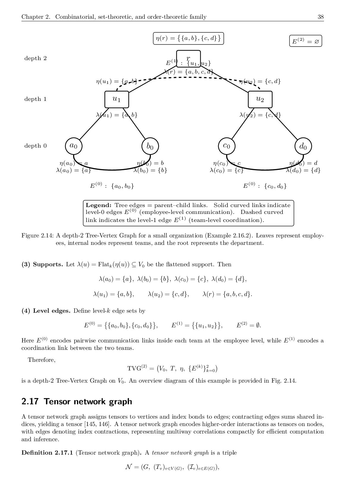
    knowledge superhypergraphs. Annals of Healthcare Systems Engineering, 877:878, 2025. [246] Takaaki Fujita. Knowledge superhypergraphs, multimodal superhypergraphs, lattice superhypergraphs, and hyperbolic su- perhypergraphs: Concepts and applications. Journal of Operational and Strategic Analytics, 3(2):95–119, 2025. [247] Zbigniew Suraj and Sibasis Bandyopadhyay. Generalized weighted fuzzy petri net in intuitionistic fuzzy environment. In 2016 IEEE International Conference on Fuzzy Systems (FUZZ-IEEE), pages 2385–2392. IEEE, 2016. [248] Xuefei Lin, Xiao Chang, Yizheng Zhang, Zhanyu Gao, and Xu Chi. Automatic construction of petri net models for compu- tational simulations of molecular interaction network. NPJ Systems Biology and Applications, 10(1):131, 2024. [249] Hua Shi, Hu-Chen Liu, Jing-Hui Wang, and Xun Mou. New linguistic z-number petri nets for knowledge acquisition and representation under large group environment. International Journal of Fuzzy Systems, 24(8):3483–3500, 2022. [250] Wei Jiang, Kai-Qing Zhou, Arezoo Sarkheyli-Hägele, and Azlan Mohd Zain. Modeling, reasoning, and application of fuzzy petri net model: a survey. Artificial Intelligence Review, 55(8):6567–6605, 2022. [251] Ya-Xuan Yu, Hua-Ping Gong, Hu-Chen Liu, and Xun Mou. Knowledge representation and reasoning using fuzzy petri nets: a literature review and bibliometric analysis. Artificial Intelligence Review, 56(7):6241–6265, 2023. [252] Jamal Khudair Madhloom, Zainab Hammoodi Noori, Sif K Ebis, Oday A Hassen, and Saad M Darwish. An information security engineering framework for modeling packet filtering firewall using neutrosophic petri nets. Computers, 12(10):202, 2023. [253] Weichao Yue, Xiaoxue Wan, Sanyi Li, Hangli Ren, and Hui He. Simplified neutrosophic petri nets used for identification of superheat degree. International Journal of Fuzzy Systems, 24(8):3431–3455, 2022. [254] Maribel Fernández, Hélène Kirchner, and Bruno Pinaud. Strategic port graph rewriting: an interactive modelling framework. Mathematical Structures in Computer Science, 29(5):615–662, 2019. [255] Maribel Fernández, Hélène Kirchner, and Bruno Pinaud. Labelled port graph–a formal structure for models and computations. Electronic Notes in Theoretical Computer Science, 338:3–21, 2018. [256] Maribel Fernández and János Varga. Finding candidate keys and 3nf via strategic port graph rewriting. In Proceedings of the 22nd International Symposium on Principles and Practice of Declarative Programming, pages 1–14, 2020. [257] Maribel Fernández, Bruno Pinaud, and János Varga. A port graph rewriting approach to relational database modelling. In International Symposium on Logic-Based Program Synthesis and Transformation, pages 211–227. Springer, 2019. [258] Dunwang Qin, Zhen Peng, and Lifeng Wu. Fchg: Fuzzy cognitive hypergraph for interpretable fault detection. Expert Systems with Applications, 255:124700, 2024. [259] Wai Yu, Douglas Reid, and Stephen Brewster. Web-based multimodal graphs for visually impaired people. In Universal Access and Assistive Technology: Proceedings of the Cambridge Workshop on UA and AT’02, pages 97–108. Springer, 2002. [260] Bruce N Walker, Michael A Nees, et al. An agenda for research and development of multimodal graphs. In Proceedings of the International Conference on Auditory Display (ICAD2005), pages 428–432, 2005. [261] Wai Yu and Stephen Brewster. Evaluation of multimodal graphs for blind people. Universal access in the information society, 2:105–124, 2003. [262] Jian Huang, Kun Jiang, Yuanyuan Pu, Zhengpeng Zhao, Qiuxia Yang, Jinjing Gu, and Dan Xu. Multimodal hypergraph network with contrastive learning for sentiment analysis. Neurocomputing, page 129566, 2025. [263] David López and Angélica Lozano. Shortest hyperpaths in a multimodal hypergraph with real-time information on some transit lines. Transportation Research Part A: Policy and Practice, 137:541–559, 2020. [264] Fuhai Chen, Yue Gao, Donglin Cao, and Rongrong Ji. Multimodal hypergraph learning for microblog sentiment prediction. In 2015 IEEE International Conference on Multimedia and Expo (ICME), pages 1–6. IEEE, 2015. [265] Takaaki Fujita. Curried graph, curried hypergraph, and curried superhypergraph functions with applications to molecular structures, 2025. [266] Grzegorz Bancerek. Curried and uncurried functions. Formalized Mathematics, 1(3):537–541, 1990. [267] Takaaki Fujita and Florentin Smarandache. A unified framework for u-structures and functorial structure: Managing super, hyper, superhyper, tree, and forest uncertain over/under/off models. Neutrosophic Sets and Systems, 91:337–380, 2025. [268] Takaaki Fujita and Florentin Smarandache. A Dynamic Survey of Fuzzy, Intuitionistic Fuzzy, Neutrosophic, , and Extensional Sets. Neutrosophic Science International Association (NSIA), 2025. [269] Mohammed Alqahtani. Intuitionistic fuzzy quasi-supergraph integration for social network decision making. International Journal of Analysis and Applications, 23:137–137, 2025. [270] T. Fujita, Muhammad Saqlain, and Muhammad Gulistan. Hierarchical network modeling with intuitionistic fuzzy superhy- pergraphs. Multicriteria Algorithms with Applications, 10(1):1–22, 2026. [271] Shouxian Zhu. Neutrosophic n-superhypernetwork: A new approach for evaluating short video communication effectiveness in media convergence. Neutrosophic Sets and Systems, 85:1004–1017, 2025. [272] E. J. Mogro, J. R. Molina, G. J. S. Canas, and P. H. Soria. Tree tobacco extract (Nicotiana glauca) as a plithogenic bioinsecticide alternative for controlling fruit fly (Drosophila immigrans) using n-superhypergraphs. Neutrosophic Sets and Systems, 74:57–65, 2024. [273] Takaaki Fujita and Florentin Smarandache. Topological generalizations of graphs: Integrating hypergraph and superhyper- graph perspectives. Turkish Journal of Mathematics and Computer Science, 17(2):322–337, 2025. [274] Ovidiu Ivanciuc. Qsar comparative study of wiener descriptors for weighted molecular graphs. Journal of chemical information and computer sciences, 40(6):1412–1422, 2000.
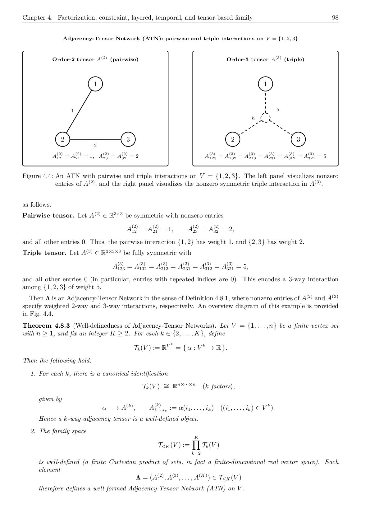
  176. Bibliography 184 [275] Sezer Sorgun and Kahraman Birgin. Vertex-edge-weighted molecular

    graphs: a study on topological indices and their relevance to physicochemical properties of drugs used in cancer treatment. Journal of Chemical Information and Modeling, 65(4):2093–2106, 2025. [276] Zoiţa Berinde. Vertex-and edge-weighted molecular graphs for amines. Revue Roumaine de Chimie, 51(11):1131, 2006. [277] Ahsanur Rahman, Christopher L Poirel, David J Badger, and TM Murali. Reverse engineering molecular hypergraphs. In Proceedings of the ACM Conference on Bioinformatics, Computational Biology and Biomedicine, pages 68–75, 2012. [278] Junwu Chen and Philippe Schwaller. Molecular hypergraph neural networks. The Journal of Chemical Physics, 160(14), 2024. [279] Hiroshi Kajino. Molecular hypergraph grammar with its application to molecular optimization. ArXiv, abs/1809.02745, 2018. [280] Hiroshi Kajino. Molecular hypergraph grammar with its application to molecular optimization. In International Conference on Machine Learning, pages 3183–3191. PMLR, 2019. [281] Takaaki Fujita. Molecular fuzzy graphs, hypergraphs, and superhypergraphs. Journal of Intelligent Decision and Computa- tional Modelling, 1(3):158–171, 2025. [282] Takaaki Fujita. An introduction and reexamination of molecular hypergraph and molecular n-superhypergraph. Asian Journal of Physical and Chemical Sciences, 13(3):1–38, 2025. [283] Zeeshan Saleem Mufti, Ali Tabraiz, Muhammad Farhan Hanif, et al. Molecular insights into tetracene through fuzzy topological indices in chemical graph theory. Chemical Papers, 79(5):2937–2953, 2025. [284] Amer Marwan El-Samman, Incé Amina Husain, Mai Huynh, Stefano De Castro, Brooke Morton, and Stijn De Baerdemacker. Global geometry of chemical graph neural network representations in terms of chemical moieties. Digital Discovery, 3(3):544– 557, 2024. [285] Muhammad Aqib, Mehar Ali Malik, Hafiz Usman Afzal, Tahzeeb Fatima, and Yasir Ali. On topological indices of some chemical graphs. Molecular Physics, page e2276386, 2023. [286] Daniel T Chang. Hypergraph: A unified and uniform definition with application to chemical hypergraph and more. arXiv preprint arXiv:2405.12235, 2024. [287] Raffaella Mulas and Dong Zhang. Spectral theory of laplace operators on chemical hypergraphs. arXiv preprint arXiv:2004.14671, 2020. [288] Elena Konstantinova. Chemical hypergraph theory. Lecture Notes from Combinatorial & Computational Mathametics Center, 2000. [289] Takaaki Fujita. Chemical hypergraph and chemical superhypergraph. Chemrxiv, 2025. [290] Takaaki Fujita. Note for biochemical/electrochemical/physicochemical hypergraphsand superhypergraphs. Information Sci- ences and Technological Innovations, 2025. [291] Jiaxuan You, Bowen Liu, Rex Ying, Vijay S. Pande, and Jure Leskovec. Graph convolutional policy network for goal-directed molecular graph generation. In Neural Information Processing Systems, 2018. [292] Anand A. Rajasekar, Karthik Raman, and Balaraman Ravindran. Goal directed molecule generation using monte carlo tree search. ArXiv, abs/2010.16399, 2020. [293] Tua A Tamba and Yul Y Nazaruddin. Data-driven construction of chemical reaction network graph using constrained lasso. In 2019 6th International Conference on Instrumentation, Control, and Automation (ICA), pages 226–230. IEEE, 2019. [294] Hans G Othmer. A graph-theoretic analysis of chemical reaction networks. Lecture Notes, Rutgers University, 1:36, 1979. [295] Gheorghe Craciun and Martin Feinberg. Multiple equilibria in complex chemical reaction networks: Ii. the species-reaction graph. SIAM Journal on Applied Mathematics, 66(4):1321–1338, 2006. [296] Azriel Rosenfeld. Fuzzy graphs. In Fuzzy sets and their applications to cognitive and decision processes, pages 77–95. Elsevier, 1975. [297] M. G. Karunambigai, R. Parvathi, and R. Buvaneswari. Arc in intuitionistic fuzzy graphs. Notes on Intuitionistic Fuzzy Sets, 17:37–47, 2011. [298] N Vinoth Kumar and G Geetha Ramani. Product intuitionistic fuzzy graph. International Journal of Computer Applications, 28(1):31–33, 2011. [299] Said Broumi, Mohamed Talea, Assia Bakali, and Florentin Smarandache. Single valued neutrosophic graphs. Journal of New theory, 10:86–101, 2016. [300] Said Broumi, Assia Bakali, Mohamed Talea, Florentin Smarandache, and Prem Kumar Singh. Properties of interval-valued neutrosophic graphs. Fuzzy Multi-criteria Decision-Making Using Neutrosophic Sets, pages 173–202, 2019. [301] Said Broumi, Mohamed Talea, Assia Bakali, and Florentin Smarandache. Interval valued neutrosophic graphs. Critical Review, XII, 2016:5–33, 2016. [302] Prem Kumar Singh et al. Dark data analysis using intuitionistic plithogenic graphs. International Journal of Neutrosophic Sciences, 16(2):80–100, 2021. [303] Fazeelat Sultana, Muhammad Gulistan, Mumtaz Ali, Naveed Yaqoob, Muhammad Khan, Tabasam Rashid, and Tauseef Ahmed. A study of plithogenic graphs: applications in spreading coronavirus disease (covid-19) globally. Journal of ambient intelligence and humanized computing, 14(10):13139–13159, 2023.