Fuzzy, Neutrosophic, and Uncertain Graph Theory: Properties and Applications

Fuzzy, Neutrosophic, and
Uncertain Graph Theory:
Properties and Applications

Transcript

2. Fuzzy, Neutrosophic, and Uncertain Graph Theory: Properties and Applications Takaaki Fujita, Florentin Smarandache Neutrosophic Science International Association (NSIA) Publishing House Gallup - Guayaquil United States of America – Ecuador 2026
3. Editor: Neutrosophic Science International Association (NSIA) Publishing House https://fs.unm.edu/NSIA/ Division of Mathematics and Sciences University of New Mexico 705 Gurley Ave., Gallup Campus NM 87301, United States of America University of Guayaquil Av. Kennedy and Av. Delta “Dr. Salvador Allende” University Campus Guayaquil 090514, Ecuador Peer-Reviewers: John Frederick D. Tapia Chemical Engineering Department, De La Salle University - Manila, 2401 Taft Avenue, Malate, Manila, Philippines Email: john.frederick.tapia@dlsu.edu.ph Darren Chong Independent researcher, Singapore Email: darrenchong2001@yahoo.com.sg Umit Cali Norwegian University of Science and Technology, NO-7491 Trondheim, Norway Email: umit.cali@ntnu.no
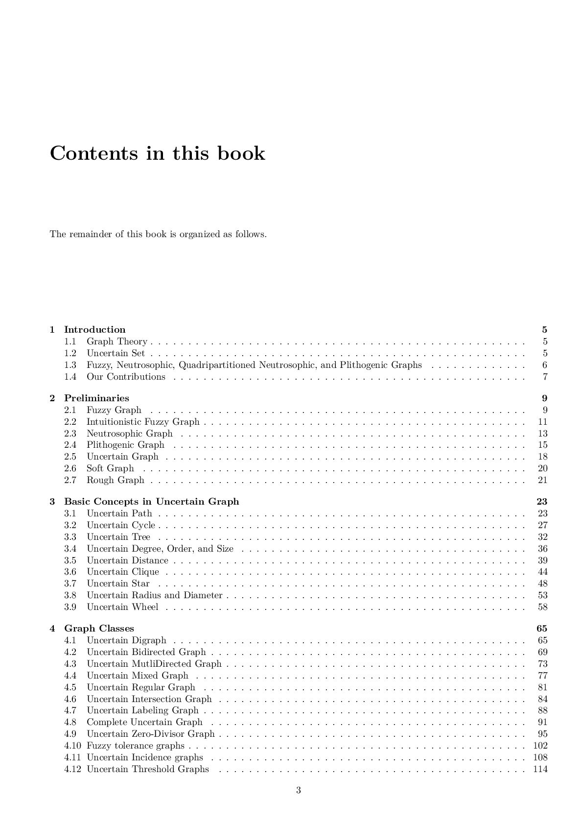
4. Contents in this book The remainder of this book is organized as follows. 1 Introduction 5 1.1 Graph Theory . . . . . . . . . . . . . . . . . . . . . . . . . . . . . . . . . . . . . . . . . . . . . . . . . . 5 1.2 Uncertain Set . . . . . . . . . . . . . . . . . . . . . . . . . . . . . . . . . . . . . . . . . . . . . . . . . . 5 1.3 Fuzzy, Neutrosophic, Quadripartitioned Neutrosophic, and Plithogenic Graphs . . . . . . . . . . . . . 6 1.4 Our Contributions . . . . . . . . . . . . . . . . . . . . . . . . . . . . . . . . . . . . . . . . . . . . . . . 7 2 Preliminaries 9 2.1 Fuzzy Graph . . . . . . . . . . . . . . . . . . . . . . . . . . . . . . . . . . . . . . . . . . . . . . . . . . 9 2.2 Intuitionistic Fuzzy Graph . . . . . . . . . . . . . . . . . . . . . . . . . . . . . . . . . . . . . . . . . . . 11 2.3 Neutrosophic Graph . . . . . . . . . . . . . . . . . . . . . . . . . . . . . . . . . . . . . . . . . . . . . . 13 2.4 Plithogenic Graph . . . . . . . . . . . . . . . . . . . . . . . . . . . . . . . . . . . . . . . . . . . . . . . 15 2.5 Uncertain Graph . . . . . . . . . . . . . . . . . . . . . . . . . . . . . . . . . . . . . . . . . . . . . . . . 18 2.6 Soft Graph . . . . . . . . . . . . . . . . . . . . . . . . . . . . . . . . . . . . . . . . . . . . . . . . . . . 20 2.7 Rough Graph . . . . . . . . . . . . . . . . . . . . . . . . . . . . . . . . . . . . . . . . . . . . . . . . . . 21 3 Basic Concepts in Uncertain Graph 23 3.1 Uncertain Path . . . . . . . . . . . . . . . . . . . . . . . . . . . . . . . . . . . . . . . . . . . . . . . . . 23 3.2 Uncertain Cycle . . . . . . . . . . . . . . . . . . . . . . . . . . . . . . . . . . . . . . . . . . . . . . . . . 27 3.3 Uncertain Tree . . . . . . . . . . . . . . . . . . . . . . . . . . . . . . . . . . . . . . . . . . . . . . . . . 32 3.4 Uncertain Degree, Order, and Size . . . . . . . . . . . . . . . . . . . . . . . . . . . . . . . . . . . . . . 36 3.5 Uncertain Distance . . . . . . . . . . . . . . . . . . . . . . . . . . . . . . . . . . . . . . . . . . . . . . . 39 3.6 Uncertain Clique . . . . . . . . . . . . . . . . . . . . . . . . . . . . . . . . . . . . . . . . . . . . . . . . 44 3.7 Uncertain Star . . . . . . . . . . . . . . . . . . . . . . . . . . . . . . . . . . . . . . . . . . . . . . . . . 48 3.8 Uncertain Radius and Diameter . . . . . . . . . . . . . . . . . . . . . . . . . . . . . . . . . . . . . . . . 53 3.9 Uncertain Wheel . . . . . . . . . . . . . . . . . . . . . . . . . . . . . . . . . . . . . . . . . . . . . . . . 58 4 Graph Classes 65 4.1 Uncertain Digraph . . . . . . . . . . . . . . . . . . . . . . . . . . . . . . . . . . . . . . . . . . . . . . . 65 4.2 Uncertain Bidirected Graph . . . . . . . . . . . . . . . . . . . . . . . . . . . . . . . . . . . . . . . . . . 69 4.3 Uncertain MutliDirected Graph . . . . . . . . . . . . . . . . . . . . . . . . . . . . . . . . . . . . . . . . 73 4.4 Uncertain Mixed Graph . . . . . . . . . . . . . . . . . . . . . . . . . . . . . . . . . . . . . . . . . . . . 77 4.5 Uncertain Regular Graph . . . . . . . . . . . . . . . . . . . . . . . . . . . . . . . . . . . . . . . . . . . 81 4.6 Uncertain Intersection Graph . . . . . . . . . . . . . . . . . . . . . . . . . . . . . . . . . . . . . . . . . 84 4.7 Uncertain Labeling Graph . . . . . . . . . . . . . . . . . . . . . . . . . . . . . . . . . . . . . . . . . . . 88 4.8 Complete Uncertain Graph . . . . . . . . . . . . . . . . . . . . . . . . . . . . . . . . . . . . . . . . . . 91 4.9 Uncertain Zero-Divisor Graph . . . . . . . . . . . . . . . . . . . . . . . . . . . . . . . . . . . . . . . . . 95 4.10 Fuzzy tolerance graphs . . . . . . . . . . . . . . . . . . . . . . . . . . . . . . . . . . . . . . . . . . . . . 102 4.11 Uncertain Incidence graphs . . . . . . . . . . . . . . . . . . . . . . . . . . . . . . . . . . . . . . . . . . 108 4.12 Uncertain Threshold Graphs . . . . . . . . . . . . . . . . . . . . . . . . . . . . . . . . . . . . . . . . . 114 3
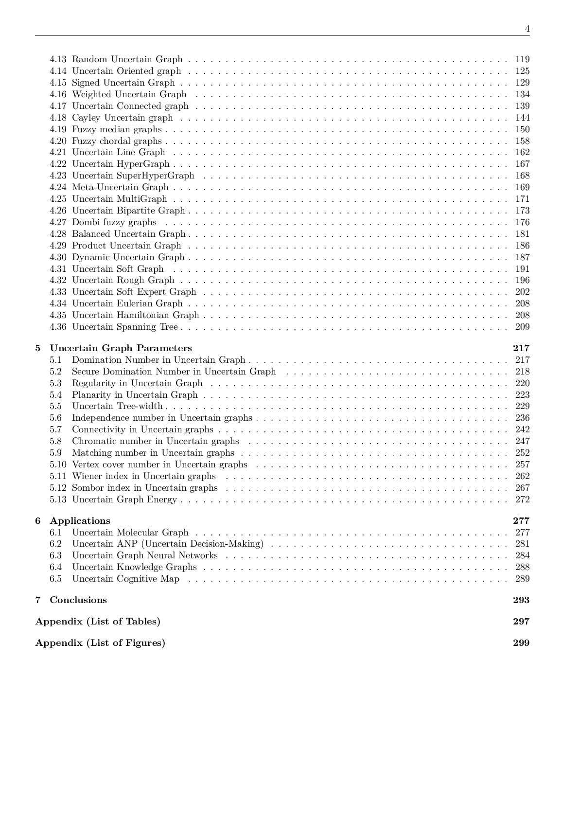
5. 4 4.13 Random Uncertain Graph . . . . . . . . . . . . . . . . . . . . . . . . . . . . . . . . . . . . . . . . . . . 119 4.14 Uncertain Oriented graph . . . . . . . . . . . . . . . . . . . . . . . . . . . . . . . . . . . . . . . . . . . 125 4.15 Signed Uncertain Graph . . . . . . . . . . . . . . . . . . . . . . . . . . . . . . . . . . . . . . . . . . . . 129 4.16 Weighted Uncertain Graph . . . . . . . . . . . . . . . . . . . . . . . . . . . . . . . . . . . . . . . . . . 134 4.17 Uncertain Connected graph . . . . . . . . . . . . . . . . . . . . . . . . . . . . . . . . . . . . . . . . . . 139 4.18 Cayley Uncertain graph . . . . . . . . . . . . . . . . . . . . . . . . . . . . . . . . . . . . . . . . . . . . 144 4.19 Fuzzy median graphs . . . . . . . . . . . . . . . . . . . . . . . . . . . . . . . . . . . . . . . . . . . . . . 150 4.20 Fuzzy chordal graphs . . . . . . . . . . . . . . . . . . . . . . . . . . . . . . . . . . . . . . . . . . . . . . 158 4.21 Uncertain Line Graph . . . . . . . . . . . . . . . . . . . . . . . . . . . . . . . . . . . . . . . . . . . . . 162 4.22 Uncertain HyperGraph . . . . . . . . . . . . . . . . . . . . . . . . . . . . . . . . . . . . . . . . . . . . . 167 4.23 Uncertain SuperHyperGraph . . . . . . . . . . . . . . . . . . . . . . . . . . . . . . . . . . . . . . . . . 168 4.24 Meta-Uncertain Graph . . . . . . . . . . . . . . . . . . . . . . . . . . . . . . . . . . . . . . . . . . . . . 169 4.25 Uncertain MultiGraph . . . . . . . . . . . . . . . . . . . . . . . . . . . . . . . . . . . . . . . . . . . . . 171 4.26 Uncertain Bipartite Graph . . . . . . . . . . . . . . . . . . . . . . . . . . . . . . . . . . . . . . . . . . . 173 4.27 Dombi fuzzy graphs . . . . . . . . . . . . . . . . . . . . . . . . . . . . . . . . . . . . . . . . . . . . . . 176 4.28 Balanced Uncertain Graph . . . . . . . . . . . . . . . . . . . . . . . . . . . . . . . . . . . . . . . . . . . 181 4.29 Product Uncertain Graph . . . . . . . . . . . . . . . . . . . . . . . . . . . . . . . . . . . . . . . . . . . 186 4.30 Dynamic Uncertain Graph . . . . . . . . . . . . . . . . . . . . . . . . . . . . . . . . . . . . . . . . . . . 187 4.31 Uncertain Soft Graph . . . . . . . . . . . . . . . . . . . . . . . . . . . . . . . . . . . . . . . . . . . . . 191 4.32 Uncertain Rough Graph . . . . . . . . . . . . . . . . . . . . . . . . . . . . . . . . . . . . . . . . . . . . 196 4.33 Uncertain Soft Expert Graph . . . . . . . . . . . . . . . . . . . . . . . . . . . . . . . . . . . . . . . . . 202 4.34 Uncertain Eulerian Graph . . . . . . . . . . . . . . . . . . . . . . . . . . . . . . . . . . . . . . . . . . . 208 4.35 Uncertain Hamiltonian Graph . . . . . . . . . . . . . . . . . . . . . . . . . . . . . . . . . . . . . . . . . 208 4.36 Uncertain Spanning Tree . . . . . . . . . . . . . . . . . . . . . . . . . . . . . . . . . . . . . . . . . . . . 209 5 Uncertain Graph Parameters 217 5.1 Domination Number in Uncertain Graph . . . . . . . . . . . . . . . . . . . . . . . . . . . . . . . . . . . 217 5.2 Secure Domination Number in Uncertain Graph . . . . . . . . . . . . . . . . . . . . . . . . . . . . . . 218 5.3 Regularity in Uncertain Graph . . . . . . . . . . . . . . . . . . . . . . . . . . . . . . . . . . . . . . . . 220 5.4 Planarity in Uncertain Graph . . . . . . . . . . . . . . . . . . . . . . . . . . . . . . . . . . . . . . . . . 223 5.5 Uncertain Tree-width . . . . . . . . . . . . . . . . . . . . . . . . . . . . . . . . . . . . . . . . . . . . . . 229 5.6 Independence number in Uncertain graphs . . . . . . . . . . . . . . . . . . . . . . . . . . . . . . . . . . 236 5.7 Connectivity in Uncertain graphs . . . . . . . . . . . . . . . . . . . . . . . . . . . . . . . . . . . . . . . 242 5.8 Chromatic number in Uncertain graphs . . . . . . . . . . . . . . . . . . . . . . . . . . . . . . . . . . . 247 5.9 Matching number in Uncertain graphs . . . . . . . . . . . . . . . . . . . . . . . . . . . . . . . . . . . . 252 5.10 Vertex cover number in Uncertain graphs . . . . . . . . . . . . . . . . . . . . . . . . . . . . . . . . . . 257 5.11 Wiener index in Uncertain graphs . . . . . . . . . . . . . . . . . . . . . . . . . . . . . . . . . . . . . . 262 5.12 Sombor index in Uncertain graphs . . . . . . . . . . . . . . . . . . . . . . . . . . . . . . . . . . . . . . 267 5.13 Uncertain Graph Energy . . . . . . . . . . . . . . . . . . . . . . . . . . . . . . . . . . . . . . . . . . . . 272 6 Applications 277 6.1 Uncertain Molecular Graph . . . . . . . . . . . . . . . . . . . . . . . . . . . . . . . . . . . . . . . . . . 277 6.2 Uncertain ANP (Uncertain Decision-Making) . . . . . . . . . . . . . . . . . . . . . . . . . . . . . . . . 281 6.3 Uncertain Graph Neural Networks . . . . . . . . . . . . . . . . . . . . . . . . . . . . . . . . . . . . . . 284 6.4 Uncertain Knowledge Graphs . . . . . . . . . . . . . . . . . . . . . . . . . . . . . . . . . . . . . . . . . 288 6.5 Uncertain Cognitive Map . . . . . . . . . . . . . . . . . . . . . . . . . . . . . . . . . . . . . . . . . . . 289 7 Conclusions 293 Appendix (List of Tables) 297 Appendix (List of Figures) 299
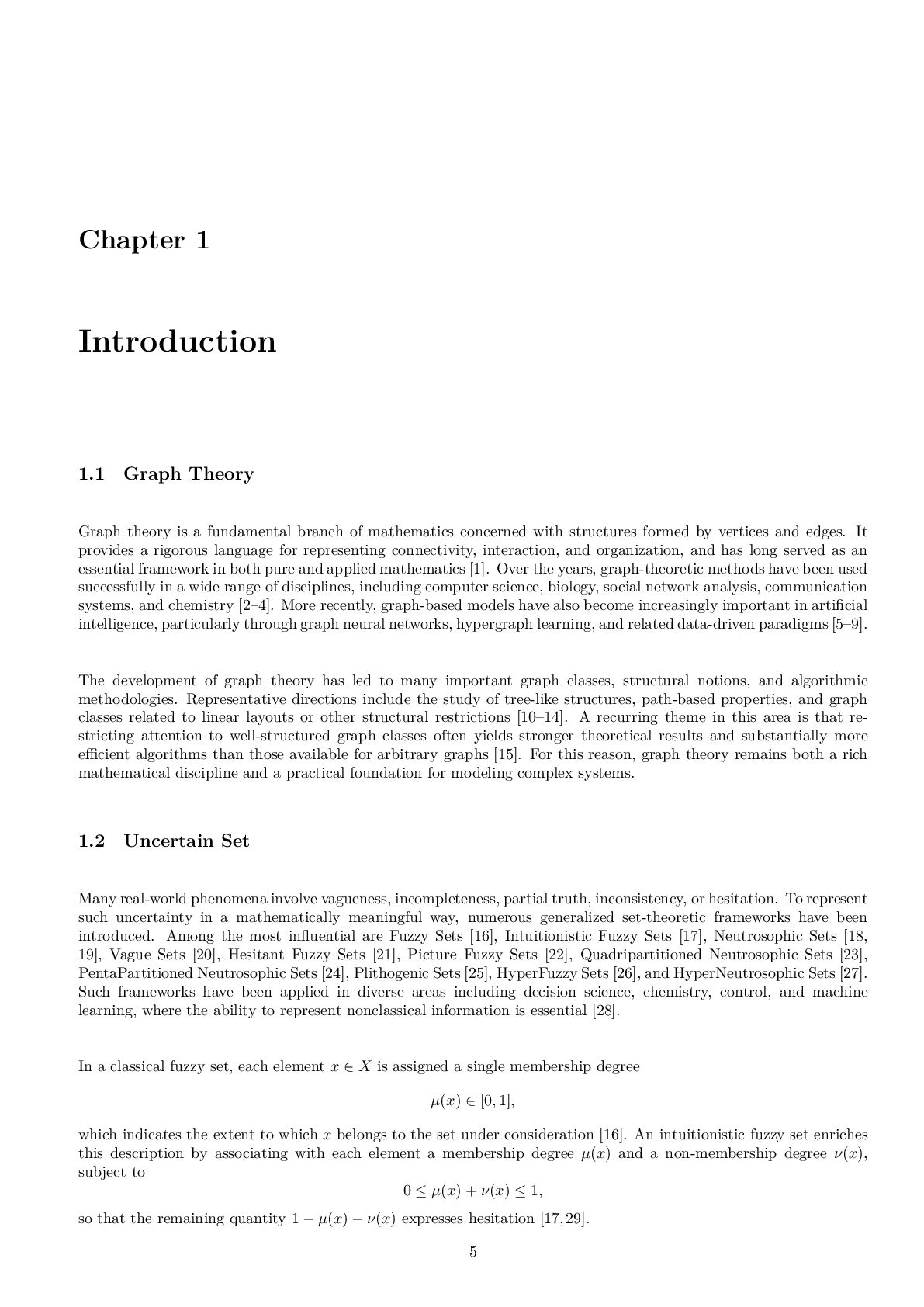
6. Chapter 1 Introduction 1.1 Graph Theory Graph theory is a fundamental branch of mathematics concerned with structures formed by vertices and edges. It provides a rigorous language for representing connectivity, interaction, and organization, and has long served as an essential framework in both pure and applied mathematics [1]. Over the years, graph-theoretic methods have been used successfully in a wide range of disciplines, including computer science, biology, social network analysis, communication systems, and chemistry [2–4]. More recently, graph-based models have also become increasingly important in artificial intelligence, particularly through graph neural networks, hypergraph learning, and related data-driven paradigms [5–9]. The development of graph theory has led to many important graph classes, structural notions, and algorithmic methodologies. Representative directions include the study of tree-like structures, path-based properties, and graph classes related to linear layouts or other structural restrictions [10–14]. A recurring theme in this area is that re- stricting attention to well-structured graph classes often yields stronger theoretical results and substantially more efficient algorithms than those available for arbitrary graphs [15]. For this reason, graph theory remains both a rich mathematical discipline and a practical foundation for modeling complex systems. 1.2 Uncertain Set Many real-world phenomena involve vagueness, incompleteness, partial truth, inconsistency, or hesitation. To represent such uncertainty in a mathematically meaningful way, numerous generalized set-theoretic frameworks have been introduced. Among the most influential are Fuzzy Sets [16], Intuitionistic Fuzzy Sets [17], Neutrosophic Sets [18, 19], Vague Sets [20], Hesitant Fuzzy Sets [21], Picture Fuzzy Sets [22], Quadripartitioned Neutrosophic Sets [23], PentaPartitioned Neutrosophic Sets [24], Plithogenic Sets [25], HyperFuzzy Sets [26], and HyperNeutrosophic Sets [27]. Such frameworks have been applied in diverse areas including decision science, chemistry, control, and machine learning, where the ability to represent nonclassical information is essential [28]. In a classical fuzzy set, each element x ∈ X is assigned a single membership degree µ(x) ∈ [0, 1], which indicates the extent to which x belongs to the set under consideration [16]. An intuitionistic fuzzy set enriches this description by associating with each element a membership degree µ(x) and a non-membership degree ν(x), subject to 0 ≤ µ(x) + ν(x) ≤ 1, so that the remaining quantity 1 − µ(x) − ν(x) expresses hesitation [17,29]. 5
7. Chapter 1. Introduction 6 A neutrosophic set further extends this viewpoint by assigning to each element a triple (T(x), I(x), F(x)), where T(x), I(x), and F(x) represent the degrees of truth, indeterminacy, and falsity, respectively. Unlike the intuitionistic fuzzy setting, these three components are not constrained to sum to 1, which makes it possible to model incomplete, inconsistent, or redundant information in a more flexible manner [29,30]. This additional expressive power has made neutrosophic frameworks important in a broad range of uncertainty-aware theories, including neutrosophic logic, probability, statistics, measure, integral, and related analytical formalisms [28,31]. Plithogenic sets provide a further refinement by describing each element through attribute values together with corre- sponding degrees of appurtenance, while also incorporating a contradiction or dissimilarity function between distinct attribute values [25,32,33]. This additional structure enables context-sensitive aggregation of heterogeneous and po- tentially conflicting evaluations, thereby generalizing and refining classical fuzzy, intuitionistic fuzzy, and neutrosophic models [31,34]. For convenience, Table 1.1 summarizes the canonical information associated with each element in several representative set extensions. Table 1.1: Representative set extensions and the canonical information stored per element. Set Type Canonical data attached to each element Fuzzy Set Membership mapping µ : X → [0, 1]. Intuitionistic Fuzzy Set Membership µ and non-membership ν with µ(x) + ν(x) ≤ 1; the gap 1 − µ(x) − ν(x) represents hesitation. Neutrosophic Set Triple (T, I, F) with T, I, F ∈ [0, 1], representing truth, indeterminacy, and falsity as mutually independent coordinates. Plithogenic Set Tuple (P, v, Pv, pdf, pCF) where pdf : P × Pv → [0, 1]s encodes s-dimensional appurte- nance and pCF : Pv × Pv → [0, 1]t is a symmetric contradiction map in [0, 1]t. 1.3 Fuzzy, Neutrosophic, Quadripartitioned Neutrosophic, and Plithogenic Graphs Since many practical systems involve uncertainty not only in attributes but also in relations, several graph-theoretic frameworks have been developed to incorporate uncertainty directly into vertices, edges, and higher-level structural information. Among these, fuzzy graphs, neutrosophic graphs, quadripartitioned neutrosophic graphs, and plithogenic graphs form an important family of uncertainty-aware network models. A fuzzy graph assigns to each vertex and each edge a membership degree in [0, 1], thereby expressing the extent to which the corresponding object belongs to the modeled structure [35,36]. In this sense, a fuzzy graph may be viewed as a graph-theoretic realization of fuzzy-set-based uncertainty [37,38]. Because many real-world relationships are inherently imprecise, fuzzy graphs have been applied to problems in social networks, decision-making, transportation systems, and related areas [35, 36]. This broad applicability has led to the development of many variants and refinements, including Intuitionistic Fuzzy Graphs [39], Bipolar Fuzzy Graphs [40], Fuzzy Planar Graphs [41], Irregular Bipolar Fuzzy Graphs [42], General Fuzzy Graphs [43,44], and Complex Hesitant Fuzzy Graphs [45]. More generally, a wide variety of graph models have been proposed to capture uncertainty and enriched relational information. These include fuzzy graphs [35, 36], vague graphs [46–48], plithogenic graphs [32, 49–51], probabilistic graphs [52–54], vague hypergraphs [55], N-graphs [56], N-hypergraphs [57], Markov graphs [58], soft graphs [59,60], hypersoft graphs [61,62], and rough graphs [63,64]. Together, these frameworks illustrate the breadth of approaches that have been developed to represent uncertainty, ambiguity, and enriched semantic structure in graph-based models. In recent years, neutrosophic graphs [65,66] and neutrosophic hypergraphs [67,68] have attracted increasing attention within the broader development of neutrosophic set theory [69, 70]. The term neutrosophic refers to a framework in which truth, indeterminacy, and falsity are treated as distinct components. From a graph-theoretic perspective, this makes it possible to represent ambiguous or inconsistent relational information more flexibly than in ordinary
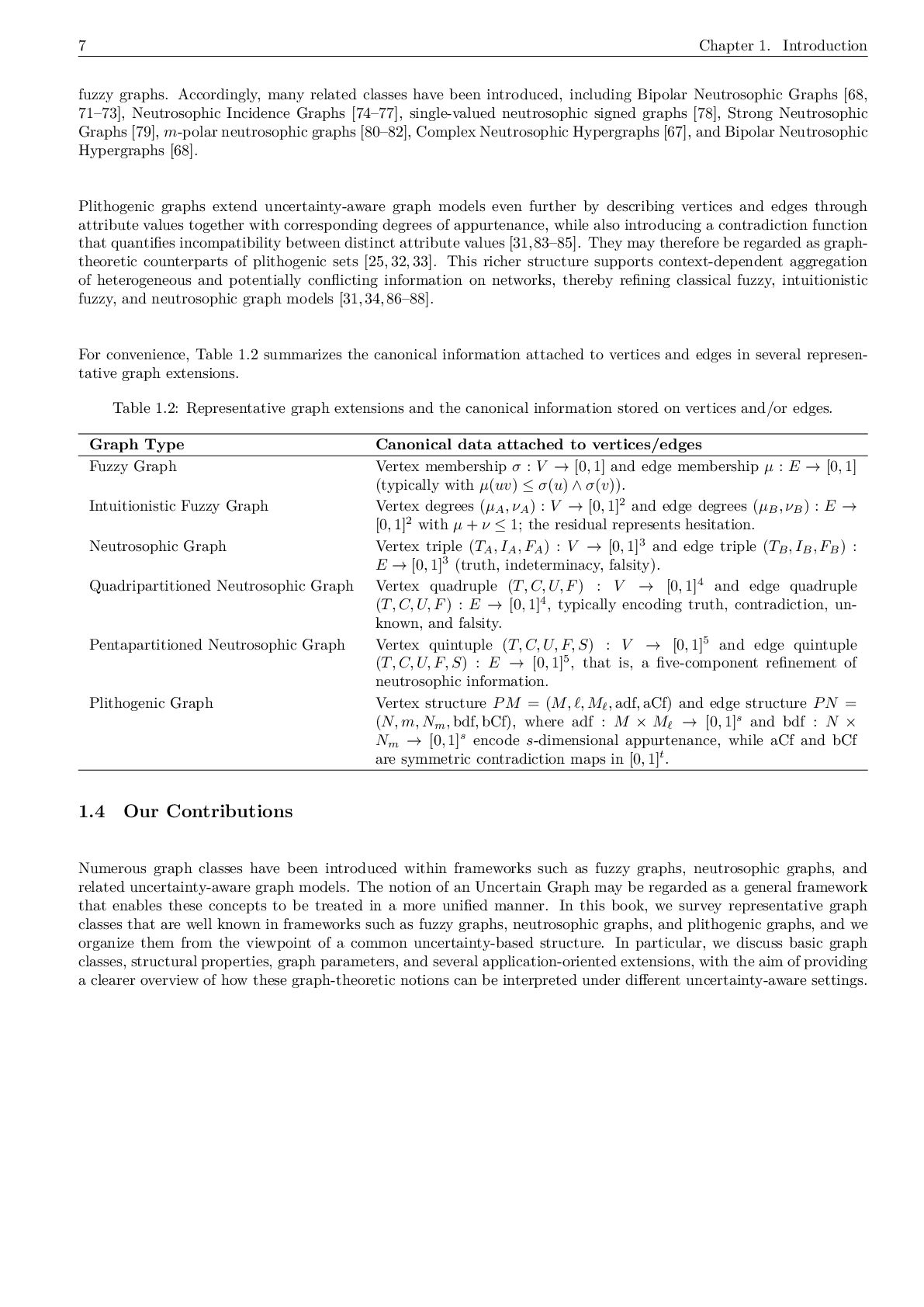
8. 7 Chapter 1. Introduction fuzzy graphs. Accordingly, many related classes have been introduced, including Bipolar Neutrosophic Graphs [68, 71–73], Neutrosophic Incidence Graphs [74–77], single-valued neutrosophic signed graphs [78], Strong Neutrosophic Graphs [79], m-polar neutrosophic graphs [80–82], Complex Neutrosophic Hypergraphs [67], and Bipolar Neutrosophic Hypergraphs [68]. Plithogenic graphs extend uncertainty-aware graph models even further by describing vertices and edges through attribute values together with corresponding degrees of appurtenance, while also introducing a contradiction function that quantifies incompatibility between distinct attribute values [31,83–85]. They may therefore be regarded as graph- theoretic counterparts of plithogenic sets [25, 32, 33]. This richer structure supports context-dependent aggregation of heterogeneous and potentially conflicting information on networks, thereby refining classical fuzzy, intuitionistic fuzzy, and neutrosophic graph models [31,34,86–88]. For convenience, Table 1.2 summarizes the canonical information attached to vertices and edges in several represen- tative graph extensions. Table 1.2: Representative graph extensions and the canonical information stored on vertices and/or edges. Graph Type Canonical data attached to vertices/edges Fuzzy Graph Vertex membership σ : V → [0, 1] and edge membership µ : E → [0, 1] (typically with µ(uv) ≤ σ(u) ∧ σ(v)). Intuitionistic Fuzzy Graph Vertex degrees (µA , νA ) : V → [0, 1]2 and edge degrees (µB , νB ) : E → [0, 1]2 with µ + ν ≤ 1; the residual represents hesitation. Neutrosophic Graph Vertex triple (TA , IA , FA ) : V → [0, 1]3 and edge triple (TB , IB , FB ) : E → [0, 1]3 (truth, indeterminacy, falsity). Quadripartitioned Neutrosophic Graph Vertex quadruple (T, C, U, F) : V → [0, 1]4 and edge quadruple (T, C, U, F) : E → [0, 1]4, typically encoding truth, contradiction, un- known, and falsity. Pentapartitioned Neutrosophic Graph Vertex quintuple (T, C, U, F, S) : V → [0, 1]5 and edge quintuple (T, C, U, F, S) : E → [0, 1]5, that is, a five-component refinement of neutrosophic information. Plithogenic Graph Vertex structure PM = (M, , M , adf, aCf) and edge structure PN = (N, m, Nm , bdf, bCf), where adf : M × M → [0, 1]s and bdf : N × Nm → [0, 1]s encode s-dimensional appurtenance, while aCf and bCf are symmetric contradiction maps in [0, 1]t. 1.4 Our Contributions Numerous graph classes have been introduced within frameworks such as fuzzy graphs, neutrosophic graphs, and related uncertainty-aware graph models. The notion of an Uncertain Graph may be regarded as a general framework that enables these concepts to be treated in a more unified manner. In this book, we survey representative graph classes that are well known in frameworks such as fuzzy graphs, neutrosophic graphs, and plithogenic graphs, and we organize them from the viewpoint of a common uncertainty-based structure. In particular, we discuss basic graph classes, structural properties, graph parameters, and several application-oriented extensions, with the aim of providing a clearer overview of how these graph-theoretic notions can be interpreted under different uncertainty-aware settings.
9. Fuzzy, Neutrosophic, and Uncertain Graph Theory: Properties and Applications Takaaki Fujita 1 ∗ and Florentin Smarandache2 1 Independent Researcher, Tokyo, Japan. 2 Email: Takaaki.fujita060@gmail.com University of New Mexico, Gallup Campus, NM 87301, USA. Email: fsmarandache@gmail.com Abstract Since many practical systems involve uncertainty not only in attributes but also in relations, several graph-theoretic frameworks have been developed to incorporate uncertainty directly into vertices, edges, and higher-level structural information. Among these, fuzzy graphs, neutrosophic graphs, and plithogenic graphs form an important family of uncertainty-aware network models. Numerous graph classes have been introduced within frameworks such as fuzzy graphs and neutrosophic graphs. The notion of an Uncertain Graph may be regarded as a new framework that enables these concepts to be considered in a unified manner. In this book, we survey graph classes that are well known in frameworks such as fuzzy graphs, neutrosophic graphs, and plithogenic graphs. Keywords: Fuzzy Graph, Intuitionistic Fuzzy Graph, Neutrosophic Graph, Plithogenic Set
10. Chapter 2 Preliminaries This chapter collects the basic notation and background used throughout the book. Except when stated otherwise, all sets are assumed to be finite. 2.1 Fuzzy Graph A fuzzy set assigns each element a membership degree between 0 and 1, modeling partial belonging and uncertainty in classification [16,89]. A fuzzy graph combines fuzzy vertex and edge membership functions, representing relationships with uncertainty and graded connectivity among nodes [35,90]. Definition 2.1.1 (Fuzzy set). [16] Let Y be a non-empty universe. A fuzzy set τ on Y is a function τ : Y −→ [0, 1], assigning to each y ∈ Y a membership value τ(y). A fuzzy relation on Y is a fuzzy subset δ of Y × Y . Given a fuzzy set τ on Y , the relation δ is said to be a fuzzy relation on τ whenever δ(y, z) ≤ min{τ(y), τ(z)}, ∀ y, z ∈ Y. Definition 2.1.2 (Fuzzy graph). [35] A fuzzy graph on a vertex set V is a pair G = (σ, µ) consisting of: • A vertex membership function σ : V → [0, 1], where σ(x) gives the degree to which x ∈ V belongs to the graph. • An edge membership function µ : V × V → [0, 1], which is a fuzzy relation on σ, satisfying µ(x, y) ≤ σ(x) ∧ σ(y), ∀ x, y ∈ V, where ∧ denotes the minimum operator. The associated crisp graph G∗ = (σ∗, µ∗) is determined by σ∗ = { x ∈ V | σ(x) > 0 }, µ∗ = { (x, y) ∈ V × V | µ(x, y) > 0 }. A fuzzy subgraph H = (σ , µ ) of G is obtained by choosing a subset X ⊆ V and defining • a restricted vertex membership σ : X → [0, 1], 9
11. Chapter 2. Preliminaries 10 • an edge membership µ : X × X → [0, 1] such that µ (x, y) ≤ σ (x) ∧ σ (y), ∀ x, y ∈ X. Example 2.1.3 (A fuzzy graph and one of its fuzzy subgraphs). Let V = {v1 , v2 , v3 , v4 }. Define a vertex-membership function σ : V → [0, 1] by σ(v1 ) = 0.9, σ(v2 ) = 0.7, σ(v3 ) = 0.5, σ(v4 ) = 0.6. Next, define an edge-membership function µ : V × V → [0, 1] by µ(v1 , v2 ) = 0.6, µ(v2 , v3 ) = 0.4, µ(v3 , v4 ) = 0.3, µ(v1 , v4 ) = 0.5, and let µ(vi , vj ) = 0 for all other unordered pairs {vi , vj } ⊆ V , with µ(vi , vj ) = µ(vj , vi ) for all i, j. Then G = (σ, µ) is a fuzzy graph, because for every edge with positive membership we have µ(v1 , v2 ) = 0.6 ≤ min{0.9, 0.7} = 0.7, µ(v2 , v3 ) = 0.4 ≤ min{0.7, 0.5} = 0.5, µ(v3 , v4 ) = 0.3 ≤ min{0.5, 0.6} = 0.5, and µ(v1 , v4 ) = 0.5 ≤ min{0.9, 0.6} = 0.6. Hence the associated crisp graph is G∗ = (V ∗, E∗), where V ∗ = {v1 , v2 , v3 , v4 }, since all vertex-memberships are positive, and E∗ = {v1 , v2 }, {v2 , v3 }, {v3 , v4 }, {v1 , v4 } , since these are exactly the pairs having positive edge-membership. Now choose X = {v1 , v2 , v4 } ⊆ V. Define a fuzzy subgraph H = (σ , µ ) on X by σ (v1 ) = 0.9, σ (v2 ) = 0.7, σ (v4 ) = 0.4, and µ (v1 , v2 ) = 0.5, µ (v1 , v4 ) = 0.3, µ (v2 , v4 ) = 0.2, with µ (x, y) = 0 for all other pairs in X × X, and µ (x, y) = µ (y, x). Again, H is a fuzzy graph, since µ (v1 , v2 ) = 0.5 ≤ min{0.9, 0.7} = 0.7, µ (v1 , v4 ) = 0.3 ≤ min{0.9, 0.4} = 0.4, and µ (v2 , v4 ) = 0.2 ≤ min{0.7, 0.4} = 0.4. Therefore H is a fuzzy subgraph of G. For reference, the illustrative figure is shown in Figure 2.1.
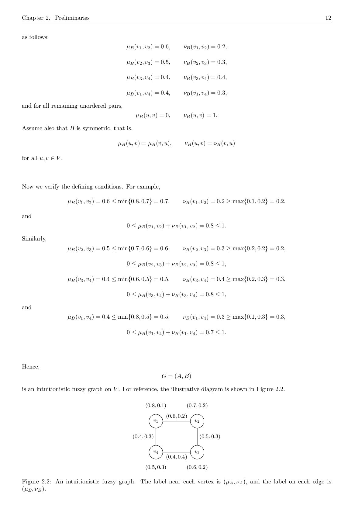
12. 11 Chapter 2. Preliminaries v1 v2 v3 v4 0.6 0.4 0.3 0.5 σ(v1 ) = 0.9 σ(v2 ) = 0.7 σ(v3 ) = 0.5 σ(v4 ) = 0.6 G = (σ, µ) v1 v2 v4 0.5 0.3 0.2 σ (v1 ) = 0.9 σ (v2 ) = 0.7 σ (v4 ) = 0.4 H = (σ , µ ) Figure 2.1: A fuzzy graph G and a fuzzy subgraph H. Vertex labels indicate the elements of V , numbers near vertices represent vertex-memberships, and numbers on edges represent edge-memberships. 2.2 Intuitionistic Fuzzy Graph An intuitionistic fuzzy set assigns each element membership and nonmembership degrees, with their sum at most one, explicitly representing hesitation and incomplete information in contexts [91,92]. An intuitionistic fuzzy graph extends a graph by assigning membership and nonmembership degrees to vertices and edges, thereby modeling uncertain relations, partial connectivity, and hesitation [93]. Definition 2.2.1 (Intuitionistic Fuzzy Graph). Let V be a nonempty vertex set. An intuitionistic fuzzy graph on V is a pair G = (A, B), where A = {(v, µA (v), νA (v)) : v ∈ V } is an intuitionistic fuzzy set on V , and B = {((u, v), µB (u, v), νB (u, v)) : u, v ∈ V } is an intuitionistic fuzzy relation on V , satisfying 0 ≤ µA (v) + νA (v) ≤ 1 for all v ∈ V, and µB (u, v) ≤ min{µA (u), µA (v)}, νB (u, v) ≥ max{νA (u), νA (v)} for all u, v ∈ V , with 0 ≤ µB (u, v) + νB (u, v) ≤ 1. Here, µA and µB denote the membership degrees, while νA and νB denote the non-membership degrees of vertices and edges, respectively. Example 2.2.2 (An intuitionistic fuzzy graph). Let V = {v1 , v2 , v3 , v4 }. Define an intuitionistic fuzzy set A = {(v, µA (v), νA (v)) : v ∈ V } on V by A = {(v1 , 0.8, 0.1), (v2 , 0.7, 0.2), (v3 , 0.6, 0.2), (v4 , 0.5, 0.3)}. Clearly, 0 ≤ µA (vi ) + νA (vi ) ≤ 1 (i = 1, 2, 3, 4), since 0.8 + 0.1 = 0.9, 0.7 + 0.2 = 0.9, 0.6 + 0.2 = 0.8, 0.5 + 0.3 = 0.8. Next, define an intuitionistic fuzzy relation B = {((u, v), µB (u, v), νB (u, v)) : u, v ∈ V }
13. Chapter 2. Preliminaries 12 as follows: µB (v1 , v2 ) = 0.6, νB (v1 , v2 ) = 0.2, µB (v2 , v3 ) = 0.5, νB (v2 , v3 ) = 0.3, µB (v3 , v4 ) = 0.4, νB (v3 , v4 ) = 0.4, µB (v1 , v4 ) = 0.4, νB (v1 , v4 ) = 0.3, and for all remaining unordered pairs, µB (u, v) = 0, νB (u, v) = 1. Assume also that B is symmetric, that is, µB (u, v) = µB (v, u), νB (u, v) = νB (v, u) for all u, v ∈ V . Now we verify the defining conditions. For example, µB (v1 , v2 ) = 0.6 ≤ min{0.8, 0.7} = 0.7, νB (v1 , v2 ) = 0.2 ≥ max{0.1, 0.2} = 0.2, and 0 ≤ µB (v1 , v2 ) + νB (v1 , v2 ) = 0.8 ≤ 1. Similarly, µB (v2 , v3 ) = 0.5 ≤ min{0.7, 0.6} = 0.6, νB (v2 , v3 ) = 0.3 ≥ max{0.2, 0.2} = 0.2, 0 ≤ µB (v2 , v3 ) + νB (v2 , v3 ) = 0.8 ≤ 1, µB (v3 , v4 ) = 0.4 ≤ min{0.6, 0.5} = 0.5, νB (v3 , v4 ) = 0.4 ≥ max{0.2, 0.3} = 0.3, 0 ≤ µB (v3 , v4 ) + νB (v3 , v4 ) = 0.8 ≤ 1, and µB (v1 , v4 ) = 0.4 ≤ min{0.8, 0.5} = 0.5, νB (v1 , v4 ) = 0.3 ≥ max{0.1, 0.3} = 0.3, 0 ≤ µB (v1 , v4 ) + νB (v1 , v4 ) = 0.7 ≤ 1. Hence, G = (A, B) is an intuitionistic fuzzy graph on V . For reference, the illustrative diagram is shown in Figure 2.2. v1 v2 v3 v4 (0.6, 0.2) (0.5, 0.3) (0.4, 0.4) (0.4, 0.3) (0.8, 0.1) (0.7, 0.2) (0.6, 0.2) (0.5, 0.3) Figure 2.2: An intuitionistic fuzzy graph. The label near each vertex is (µA , νA ), and the label on each edge is (µB , νB ).
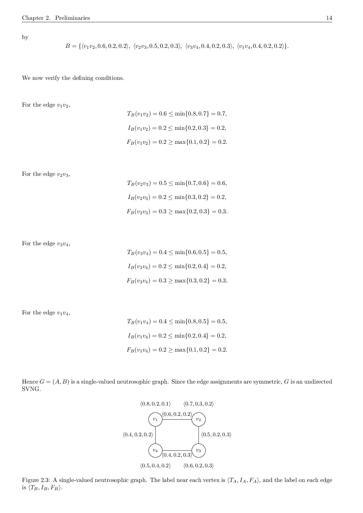
14. 13 Chapter 2. Preliminaries 2.3 Neutrosophic Graph A Single-Valued Neutrosophic Graph assigns truth, indeterminacy, and falsity degrees to vertices and edges, extending classical graphs [19,76,94,95]. Definition 2.3.1 (Single-Valued Neutrosophic Graph). [19] Let G∗ = (V, E) be a crisp (classical) graph, where V is the vertex set and E ⊆ V × V the edge set. A single-valued neutrosophic graph (SVNG) on G∗ is defined as a pair G = (A, B), where • A = { v, TA (v), IA (v), FA (v) : v ∈ V } is the single-valued neutrosophic vertex set, with TA , IA , FA : V → [0, 1], denoting respectively the truth-membership, indeterminacy-membership, and falsity-membership functions of vertices, such that for every v ∈ V , 0 ≤ TA (v) + IA (v) + FA (v) ≤ 3. • B = { uv, TB (uv), IB (uv), FB (uv) : uv ∈ E} is the single-valued neutrosophic edge set, with TB , IB , FB : E → [0, 1], satisfying for all u, v ∈ V with uv ∈ E: TB (uv) ≤ min{TA (u), TA (v)}, IB (uv) ≤ min{IA (u), IA (v)}, FB (uv) ≥ max{FA (u), FA (v)}. If B is symmetric, G = (A, B) is called an undirected SVNG; otherwise, it is a directed SVNG. Example 2.3.2 (A single-valued neutrosophic graph). Let the underlying crisp graph be G∗ = (V, E), where V = {v1 , v2 , v3 , v4 } and E = {v1 v2 , v2 v3 , v3 v4 , v1 v4 }. Define the single-valued neutrosophic vertex set A = { v, TA (v), IA (v), FA (v) : v ∈ V } by A = { v1 , 0.8, 0.2, 0.1 , v2 , 0.7, 0.3, 0.2 , v3 , 0.6, 0.2, 0.3 , v4 , 0.5, 0.4, 0.2 }. Then, for each vertex vi ∈ V , 0 ≤ TA (vi ) + IA (vi ) + FA (vi ) ≤ 3. Indeed, 0.8 + 0.2 + 0.1 = 1.1, 0.7 + 0.3 + 0.2 = 1.2, 0.6 + 0.2 + 0.3 = 1.1, 0.5 + 0.4 + 0.2 = 1.1. Next, define the single-valued neutrosophic edge set B = { uv, TB (uv), IB (uv), FB (uv) : uv ∈ E}
15. Chapter 2. Preliminaries 14 by B = { v1 v2 , 0.6, 0.2, 0.2 , v2 v3 , 0.5, 0.2, 0.3 , v3 v4 , 0.4, 0.2, 0.3 , v1 v4 , 0.4, 0.2, 0.2 }. We now verify the defining conditions. For the edge v1 v2 , TB (v1 v2 ) = 0.6 ≤ min{0.8, 0.7} = 0.7, IB (v1 v2 ) = 0.2 ≤ min{0.2, 0.3} = 0.2, FB (v1 v2 ) = 0.2 ≥ max{0.1, 0.2} = 0.2. For the edge v2 v3 , TB (v2 v3 ) = 0.5 ≤ min{0.7, 0.6} = 0.6, IB (v2 v3 ) = 0.2 ≤ min{0.3, 0.2} = 0.2, FB (v2 v3 ) = 0.3 ≥ max{0.2, 0.3} = 0.3. For the edge v3 v4 , TB (v3 v4 ) = 0.4 ≤ min{0.6, 0.5} = 0.5, IB (v3 v4 ) = 0.2 ≤ min{0.2, 0.4} = 0.2, FB (v3 v4 ) = 0.3 ≥ max{0.3, 0.2} = 0.3. For the edge v1 v4 , TB (v1 v4 ) = 0.4 ≤ min{0.8, 0.5} = 0.5, IB (v1 v4 ) = 0.2 ≤ min{0.2, 0.4} = 0.2, FB (v1 v4 ) = 0.2 ≥ max{0.1, 0.2} = 0.2. Hence G = (A, B) is a single-valued neutrosophic graph. Since the edge assignments are symmetric, G is an undirected SVNG. v1 v2 v3 v4 0.6, 0.2, 0.2 0.5, 0.2, 0.3 0.4, 0.2, 0.3 0.4, 0.2, 0.2 0.8, 0.2, 0.1 0.7, 0.3, 0.2 0.6, 0.2, 0.3 0.5, 0.4, 0.2 Figure 2.3: A single-valued neutrosophic graph. The label near each vertex is TA , IA , FA , and the label on each edge is TB , IB , FB .
16. 15 Chapter 2. Preliminaries 2.4 Plithogenic Graph A plithogenic set models elements through attribute values, appurtenance degrees, and contradiction degrees, cap- turing multi-valued, attribute-dependent uncertainty, diversity, inconsistency, and context in complex systems for- mally [32,49]. A plithogenic graph extends graphs using attribute-based appurtenance and contradiction degrees on vertices and edges, representing heterogeneous, context-sensitive, multi-valued relationships under uncertainty and inconsistency formally [83]. Definition 2.4.1 (Plithogenic Set). [32,49] Let S be a universal set and P ⊆ S a nonempty subset. A Plithogenic Set is a quintuple PS = (P, v, Pv, pdf, pCF), where • v is an attribute, • Pv is the set of possible values of the attribute v, • pdf : P × Pv → [0, 1]s is the Degree of Appurtenance Function (DAF),1 • pCF : Pv × Pv → [0, 1]t is the Degree of Contradiction Function (DCF). The DCF satisfies, for all a, b ∈ Pv, Reflexivity: pCF(a, a) = 0, Symmetry: pCF(a, b) = pCF(b, a). Here s ∈ N is the appurtenance dimension and t ∈ N the contradiction dimension. Definition 2.4.2 (Plithogenic Graph). (cf. [33, 83]) Let G = (V, E) be a crisp (simple, undirected) graph with E ⊆ {{x, y} : x, y ∈ V, x = y}. A plithogenic graph is a pair PG = (PM, PN), where the vertex and edge components are specified as follows. Vertex component. PM = (M, , ML, adf, aCf), with • M ⊆ V a chosen vertex subset; • an attribute attached to vertices; • ML the set of possible values of ; • adf : M × ML → [0, 1]s the vertex DAF; • aCf : ML × ML → [0, 1]t the vertex DCF. Edge component. PN = (N, m, ML , bdf, bCf), with 1In the literature, DAF is defined in slightly different ways: some variants use powerset–valued constructions, others the simple cube [0, 1]s. We adopt the latter (classical) form here; cf. [96].
17. Chapter 2. Preliminaries 16 • N ⊆ E a chosen edge subset; • m an attribute attached to edges; • ML the set of possible values of m; • bdf : N × ML → [0, 1]s the edge DAF; • bCf : ML × ML → [0, 1]t the edge DCF. All inequalities in [0, 1]k are interpreted componentwise. Fix s, t ∈ N. The following axioms are required. (A1) Edge–vertex compatibility (appurtenance bound). For all {x, y} ∈ N and a, b ∈ ML, bdf {x, y}, (a, b) ≤ min adf(x, a), adf(y, b) . (2.1) (A2) Contradiction consistency (edge vs. vertices). For all (a, b), (c, d) ∈ ML , bCf (a, b), (c, d) ≤ min aCf(a, c), aCf(b, d) . (2.2) (A3) Reflexivity and symmetry of DCF. aCf(u, u) = 0, aCf(u, v) = aCf(v, u) (∀ u, v ∈ ML), bCf(u, u) = 0, bCf(u, v) = bCf(v, u) (∀ u, v ∈ ML ). When s = t = 1, all maps are scalar-valued in [0, 1] and (2.1)–(2.2) are scalar inequalities. Example 2.4.3 (A plithogenic graph). We construct a simple scalar-valued plithogenic graph, so we take s = t = 1. Let the underlying crisp graph be G = (V, E), V = {v1 , v2 , v3 }, E = {v1 , v2 }, {v2 , v3 } . We use the vertex attribute = reliability level, with possible values ML = {H, L}, where H means high and L means low. We also use the edge attribute m = interaction type, and we take ML = ML × ML = {(H, H), (H, L), (L, H), (L, L)}. Define the vertex component PM = (M, , ML, adf, aCf), where M = V. Let the vertex degree-of-appurtenance function adf : M × ML → [0, 1]
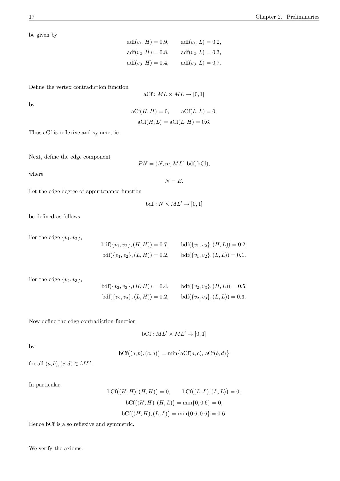
18. 17 Chapter 2. Preliminaries be given by adf(v1 , H) = 0.9, adf(v1 , L) = 0.2, adf(v2 , H) = 0.8, adf(v2 , L) = 0.3, adf(v3 , H) = 0.4, adf(v3 , L) = 0.7. Define the vertex contradiction function aCf : ML × ML → [0, 1] by aCf(H, H) = 0, aCf(L, L) = 0, aCf(H, L) = aCf(L, H) = 0.6. Thus aCf is reflexive and symmetric. Next, define the edge component PN = (N, m, ML , bdf, bCf), where N = E. Let the edge degree-of-appurtenance function bdf : N × ML → [0, 1] be defined as follows. For the edge {v1 , v2 }, bdf({v1 , v2 }, (H, H)) = 0.7, bdf({v1 , v2 }, (H, L)) = 0.2, bdf({v1 , v2 }, (L, H)) = 0.2, bdf({v1 , v2 }, (L, L)) = 0.1. For the edge {v2 , v3 }, bdf({v2 , v3 }, (H, H)) = 0.4, bdf({v2 , v3 }, (H, L)) = 0.5, bdf({v2 , v3 }, (L, H)) = 0.2, bdf({v2 , v3 }, (L, L)) = 0.3. Now define the edge contradiction function bCf : ML × ML → [0, 1] by bCf (a, b), (c, d) = min aCf(a, c), aCf(b, d) for all (a, b), (c, d) ∈ ML . In particular, bCf (H, H), (H, H) = 0, bCf (L, L), (L, L) = 0, bCf (H, H), (H, L) = min{0, 0.6} = 0, bCf (H, H), (L, L) = min{0.6, 0.6} = 0.6. Hence bCf is also reflexive and symmetric. We verify the axioms.
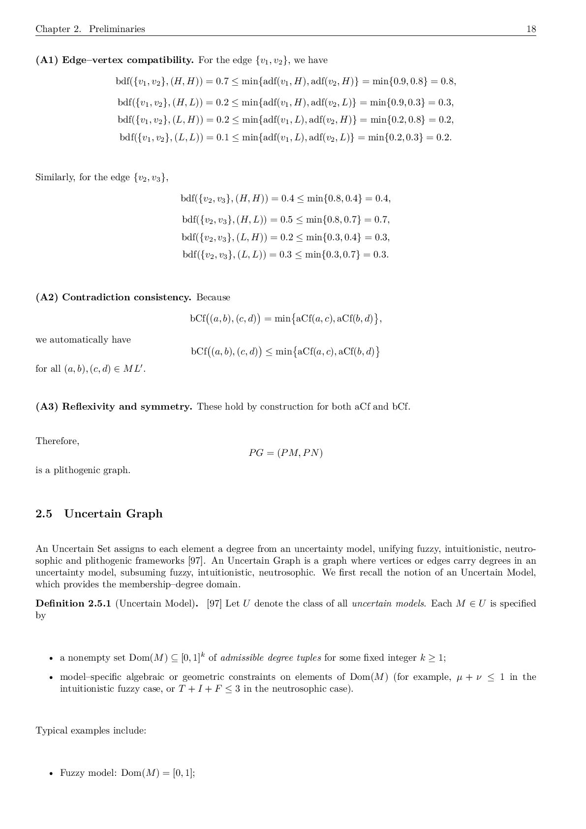
19. Chapter 2. Preliminaries 18 (A1) Edge–vertex compatibility. For the edge {v1 , v2 }, we have bdf({v1 , v2 }, (H, H)) = 0.7 ≤ min{adf(v1 , H), adf(v2 , H)} = min{0.9, 0.8} = 0.8, bdf({v1 , v2 }, (H, L)) = 0.2 ≤ min{adf(v1 , H), adf(v2 , L)} = min{0.9, 0.3} = 0.3, bdf({v1 , v2 }, (L, H)) = 0.2 ≤ min{adf(v1 , L), adf(v2 , H)} = min{0.2, 0.8} = 0.2, bdf({v1 , v2 }, (L, L)) = 0.1 ≤ min{adf(v1 , L), adf(v2 , L)} = min{0.2, 0.3} = 0.2. Similarly, for the edge {v2 , v3 }, bdf({v2 , v3 }, (H, H)) = 0.4 ≤ min{0.8, 0.4} = 0.4, bdf({v2 , v3 }, (H, L)) = 0.5 ≤ min{0.8, 0.7} = 0.7, bdf({v2 , v3 }, (L, H)) = 0.2 ≤ min{0.3, 0.4} = 0.3, bdf({v2 , v3 }, (L, L)) = 0.3 ≤ min{0.3, 0.7} = 0.3. (A2) Contradiction consistency. Because bCf (a, b), (c, d) = min aCf(a, c), aCf(b, d) , we automatically have bCf (a, b), (c, d) ≤ min aCf(a, c), aCf(b, d) for all (a, b), (c, d) ∈ ML . (A3) Reflexivity and symmetry. These hold by construction for both aCf and bCf. Therefore, PG = (PM, PN) is a plithogenic graph. 2.5 Uncertain Graph An Uncertain Set assigns to each element a degree from an uncertainty model, unifying fuzzy, intuitionistic, neutro- sophic and plithogenic frameworks [97]. An Uncertain Graph is a graph where vertices or edges carry degrees in an uncertainty model, subsuming fuzzy, intuitionistic, neutrosophic. We first recall the notion of an Uncertain Model, which provides the membership–degree domain. Definition 2.5.1 (Uncertain Model). [97] Let U denote the class of all uncertain models. Each M ∈ U is specified by • a nonempty set Dom(M) ⊆ [0, 1]k of admissible degree tuples for some fixed integer k ≥ 1; • model–specific algebraic or geometric constraints on elements of Dom(M) (for example, µ + ν ≤ 1 in the intuitionistic fuzzy case, or T + I + F ≤ 3 in the neutrosophic case). Typical examples include: • Fuzzy model: Dom(M) = [0, 1];
20. 19 Chapter 2. Preliminaries • Intuitionistic fuzzy model: Dom(M) = {(µ, ν) ∈ [0, 1]2 | µ + ν ≤ 1}; • Neutrosophic model: Dom(M) = {(T, I, F) ∈ [0, 1]3 | 0 ≤ T + I + F ≤ 3}; • Plithogenic model, and many other extensions. Definition 2.5.2 (Uncertain Set (U-Set)). [97] Let X be a nonempty universe, and let M be a fixed uncertain model with degree–domain Dom(M) ⊆ [0, 1]k. An Uncertain Set of type M (or U-Set for short) on X is a pair U = (X, µM ), where µM : X −→ Dom(M) is called the uncertainty–degree function (or membership map) of U. For x ∈ X, the value µM (x) ∈ Dom(M) encodes the degree(s) to which x belongs to the uncertain set, according to the model M. Remark 2.5.3. Special cases: • If M is the fuzzy model and Dom(M) = [0, 1], then µM : X → [0, 1] is a usual fuzzy membership function and U is a fuzzy set. • If M is neutrosophic, then µM (x) = (T(x), I(x), F(x)) gives a neutrosophic set. • Other choices of M recover intuitionistic fuzzy sets, picture fuzzy sets, plithogenic sets, and so on. As noted in the remark, various generalizations are possible. For reference, Table 2.1 presents a catalogue of uncertainty-set families (U-Sets) organized by the dimension k of the degree-domain Dom(M) ⊆ [0, 1]k (cf. [98]). Table 2.1: A catalogue of uncertainty-set families (U-Sets) by the dimension k of the degree-domain Dom(M) ⊆ [0, 1]k [98]. k note Representative U-Set model(s) whose degree-domain is a subset of [0, 1]k 1 Fuzzy Set [16,36]; N-Fuzzy Set [99–101] Shadowed Set [102–104] 2 Intuitionistic Fuzzy Set [17,92]; Vague Set [20,55]; Bipolar Fuzzy Set (two-component description) [105]; Variable Fuzzy Set [106–108]; Paraconsistent Fuzzy Set [109,110]; Bifuzzy Set [111,112] 3 Single-Valued Neutrosophic Set [113,114]; Picture Fuzzy Set [22,115]; Spherical Fuzzy Set [116,117]; Tripolar Fuzzy Set (three-component formalisms) [118–120]; Neutrosophic Vague Set [69,121] 4 Quadripartitioned Neutrosophic Set [23,122]; Double-Valued Neutrosophic Set [123,124]; Dual Hes- itant Fuzzy Set [125,126]; Ambiguous Set [127–129]; Turiyam Neutrosophic Set [130–133] 5 Pentapartitioned Neutrosophic Set [134–136]; Triple-Valued Neutrosophic Set [137–139] 6 Hexapartitioned Neutrosophic Set; Quadruple-Valued Neutrosophic Set [138,140] 7 Heptapartitioned Neutrosophic Set; Quintuple-Valued Neutrosophic Set [138,141,142] 8 Octapartitioned Neutrosophic Set [143,144] 9 Nonapartitioned Neutrosophic Set [143,144] n (n ≥ 1) Multi-valued (Fuzzy) Sets [145]; MultiFuzzy Set [146]; n-Refined Fuzzy Set [147,148] 2n (n ≥ 1) n-Refined Intuitionistic Fuzzy Set [148]; Multi-Intuitionistic Fuzzy Set [146] 3n (n ≥ 1) n-Refined Neutrosophic Set [148]; Multi-Neutrosophic Set [146,149] Reading guide. In the U-Set scheme [97], each model M is specified by a degree-domain Dom(M) ⊆ [0, 1]k and a membership map µM : X → Dom(M). The table groups representative families by the ambient dimension k (i.e., how many numerical components are stored per element). (a) A widely cited viewpoint is that neutrosophic sets provide a unifying umbrella covering several earlier multi-component fuzzy models (and their generalizations); see [150]. (b) Ambiguous sets are commonly presented as subclasses of certain four-component neutrosophic families; see [23,122,129]. (c) Turiyam neutrosophic sets are reported as subclasses of quadripartitioned neutrosophic sets; see [151]. The definitions and related concepts of Uncertain Graphs are presented below.
21. Chapter 2. Preliminaries 20 Definition 2.5.4 (Uncertain Graph). Let G = (V, E) be a (finite, undirected, loopless) graph and let M be an uncertain model with degree–domain Dom(M). An Uncertain Graph of type M is a triple GM = (V, E, µM ), where µM : V ∪ E −→ Dom(M) assigns to each vertex v ∈ V and each edge e ∈ E an uncertainty degree µM (v) or µM (e) in Dom(M). Optionally, one may impose model–specific consistency conditions between vertex and edge degrees (for instance, µM (e) bounded in terms of µM (u) and µM (v) for e = {u, v} in fuzzy or intuitionistic fuzzy graph models), but these constraints are encoded in the choice of M and are not fixed at the level of this general definition. Remark 2.5.5. Again, particular choices of M recover well–known graph models: • Fuzzy graph (when M is fuzzy and µM : V ∪ E → [0, 1]); • Intuitionistic fuzzy graph, neutrosophic graph, plithogenic graph, etc., for the corresponding models M. As a reference, Table 2.2 presents a catalogue of uncertainty-graph families (Uncertain Graphs) organised by the dimension k of the degree-domain Dom(M) ⊆ [0, 1]k. Table 2.2: A catalogue of uncertainty-graph families (Uncertain Graphs) by the dimension k of the degree-domain Dom(M) ⊆ [0, 1]k. k Representative uncertainty-graph type(s) GM = (V, E, µM ) with µM : V ∪ E → Dom(M) ⊆ [0, 1]k 1 Fuzzy graph; N-graph; shadowed-graph variants 2 Intuitionistic fuzzy graph [152]; vague graph [153]; bipolar fuzzy graph [40]; intuitionistic evidence graph; variable fuzzy graph; paraconsistent fuzzy graph; bifuzzy graph [154,155] 3 Neutrosophic graph [19](a); hesitant fuzzy graph [156]; tripolar fuzzy graph; three-way fuzzy graph; picture fuzzy graph [157,158]; spherical fuzzy graph [116]; inconsistent intuitionistic fuzzy graph; ternary fuzzy / neutrosophic- fuzzy graph; neutrosophic vague graph 4 Quadripartitioned neutrosophic graph [159, 160]; double-valued neutrosophic graph [123]; dual hesitant fuzzy graph [161]; ambiguous graph(b); local-neutrosophic graph; support-neutrosophic graph; turiyam neutrosophic graph [162](c) 5 Pentapartitioned neutrosophic graph [163]; triple-valued neutrosophic graph 6 Hexapartitioned neutrosophic graph; quadruple-valued neutrosophic graph 7 Heptapartitioned neutrosophic graph [164]; quintuple-valued neutrosophic graph 8 Octapartitioned neutrosophic graph 9 Nonapartitioned neutrosophic graph n n-refined fuzzy graph; multi-valued (fuzzy) graphs; multi-fuzzy graphs [165] 2n n-refined intuitionistic fuzzy graph; multi-intuitionistic fuzzy graphs 3n n-refined neutrosophic graph; multi-neutrosophic graphs (a) Neutrosophic graph models are often treated as broad frameworks that can specialize to many degree-based graph formalisms under suitable constraints. (b) Ambiguous-graph models are commonly presented as subclasses of certain quadripartitioned and also double-valued neutrosophic graph models. (c) Turiyam neutrosophic graphs are reported as subclasses of certain quadripartitioned neutrosophic graph models. 2.6 Soft Graph Soft graph is a parameterized graph structure assigning to each parameter a subgraph, enabling flexible modeling of systems whose relations vary across contexts and scenarios. Definition 2.6.1 (Soft Graph). Let G∗ = (V, E) be a simple graph, and let A be a nonempty set of parameters. A soft graph over G∗ is a quadruple G = (G∗, F, K, A), where F : A → P(V ), K : A → P(E), such that, for every a ∈ A, the pair H(a) = F(a), K(a) is a subgraph of G∗.
22. 21 Chapter 2. Preliminaries 2.7 Rough Graph A rough graph represents a graph through lower and upper approximation graphs under an equivalence relation, thereby modeling indiscernibility, vagueness, and boundary uncertainty structurally formally [166,167]. Definition 2.7.1 (Rough Graph). Let U = (V, E) be a universe graph, and let R be an equivalence relation on E, inducing edge equivalence classes [e]R for e ∈ E. For a graph T = (W, X) with W ⊆ V and X ⊆ E, define R(X) = { e ∈ E : [e]R ⊆ X }, R(X) = { e ∈ E : [e]R ∩ X = ∅ }. Then the pair R(T), R(T) = (W, R(X)), (W, R(X)) is called the rough graph associated with T. If X is not a union of R-equivalence classes, then T is said to be an R-rough graph.
23. Chapter 2. Preliminaries 22
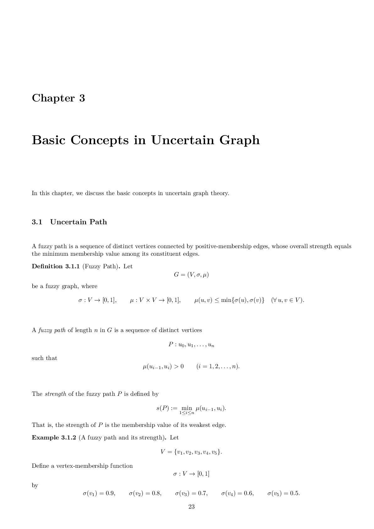
24. Chapter 3 Basic Concepts in Uncertain Graph In this chapter, we discuss the basic concepts in uncertain graph theory. 3.1 Uncertain Path A fuzzy path is a sequence of distinct vertices connected by positive-membership edges, whose overall strength equals the minimum membership value among its constituent edges. Definition 3.1.1 (Fuzzy Path). Let G = (V, σ, µ) be a fuzzy graph, where σ : V → [0, 1], µ : V × V → [0, 1], µ(u, v) ≤ min{σ(u), σ(v)} (∀ u, v ∈ V ). A fuzzy path of length n in G is a sequence of distinct vertices P : u0 , u1 , . . . , un such that µ(ui−1 , ui ) > 0 (i = 1, 2, . . . , n). The strength of the fuzzy path P is defined by s(P) := min 1≤i≤n µ(ui−1 , ui ). That is, the strength of P is the membership value of its weakest edge. Example 3.1.2 (A fuzzy path and its strength). Let V = {v1 , v2 , v3 , v4 , v5 }. Define a vertex-membership function σ : V → [0, 1] by σ(v1 ) = 0.9, σ(v2 ) = 0.8, σ(v3 ) = 0.7, σ(v4 ) = 0.6, σ(v5 ) = 0.5. 23
25. Chapter 3. Basic Concepts in Uncertain Graph 24 Next, define an edge-membership function µ : V × V → [0, 1] by µ(v1 , v2 ) = 0.6, µ(v2 , v3 ) = 0.5, µ(v3 , v4 ) = 0.4, µ(v2 , v5 ) = 0.3, µ(v4 , v5 ) = 0.2, and let µ(u, v) = 0 for all other unordered pairs {u, v} ⊆ V , with µ(u, v) = µ(v, u) for all u, v ∈ V . Then G = (V, σ, µ) is a fuzzy graph, since each positive edge-membership satisfies the required bound. For example, µ(v1 , v2 ) = 0.6 ≤ min{0.9, 0.8} = 0.8, µ(v2 , v3 ) = 0.5 ≤ min{0.8, 0.7} = 0.7, µ(v3 , v4 ) = 0.4 ≤ min{0.7, 0.6} = 0.6. Now consider the sequence of distinct vertices P : v1 , v2 , v3 , v4 . Since µ(v1 , v2 ) > 0, µ(v2 , v3 ) > 0, µ(v3 , v4 ) > 0, the sequence P is a fuzzy path of length 3. Its strength is s(P) = min µ(v1 , v2 ), µ(v2 , v3 ), µ(v3 , v4 ) = min{0.6, 0.5, 0.4} = 0.4. Hence the strength of the fuzzy path P is 0.4, which is the membership value of its weakest edge. An illustrative diagram is shown in Figure 3.1. v1 v2 v3 v4 v5 0.6 0.5 0.4 0.3 0.2 σ(v1 ) = 0.9 σ(v2 ) = 0.8 σ(v3 ) = 0.7 σ(v4 ) = 0.6 σ(v5 ) = 0.5 Figure 3.1: A fuzzy graph containing the fuzzy path P : v1 , v2 , v3 , v4 . The numbers on vertices indicate vertex- memberships, and the numbers on edges indicate edge-memberships. An uncertain path is a sequence of distinct vertices joined by support edges in an uncertain graph, together with a model-dependent path strength. Definition 3.1.3 (Path-Evaluable Uncertain Model). Let M be an uncertain model with degree-domain Dom(M) ⊆ [0, 1]k. We say that M is path-evaluable if it is equipped with:
26. 25 Chapter 3. Basic Concepts in Uncertain Graph 1. a distinguished element 0M ∈ Dom(M), called the zero degree; 2. for each integer n ≥ 1, a map Ψ(n) M : Dom(M)n −→ Dom(M), called the path-strength operator of length n. Definition 3.1.4 (Uncertain Path). Let M be a path-evaluable uncertain model with degree-domain Dom(M) ⊆ [0, 1]k, zero degree 0M ∈ Dom(M), and path-strength operators Ψ(n) M : Dom(M)n → Dom(M) (n ≥ 1). Let GM = (V, E, σM , ηM ) be an Uncertain Graph of type M, where σM : V → Dom(M), ηM : E → Dom(M). Define the support edge set by E∗(GM ) := { e ∈ E | ηM (e) = 0M }. An Uncertain Path of length n in GM is a sequence of distinct vertices P : u0 , u1 , . . . , un such that {ui−1 , ui } ∈ E∗(GM ) (i = 1, 2, . . . , n). The strength of the uncertain path P is defined by sM (P) := Ψ(n) M ηM ({u0 , u1 }), ηM ({u1 , u2 }), . . . , ηM ({un−1 , un }) . Theorem 3.1.5 (Well-definedness of Uncertain Path). Let M be a path-evaluable uncertain model with degree-domain Dom(M) ⊆ [0, 1]k, zero degree 0M ∈ Dom(M), and path-strength operators Ψ(n) M : Dom(M)n → Dom(M) (n ≥ 1). Let GM = (V, E, σM , ηM ) be an Uncertain Graph of type M. Then:
27. Chapter 3. Basic Concepts in Uncertain Graph 26 1. the support edge set E∗(GM ) = { e ∈ E | ηM (e) = 0M } is well-defined; 2. the statement “P : u0 , u1 , . . . , un is an Uncertain Path of length n” is well-defined; 3. for every Uncertain Path P : u0 , u1 , . . . , un , the quantity sM (P) = Ψ(n) M ηM ({u0 , u1 }), ηM ({u1 , u2 }), . . . , ηM ({un−1 , un }) is well-defined. Hence the notions of uncertain path and uncertain path strength are well-defined. Proof. Since M is an uncertain model, its degree-domain Dom(M) is fixed. Since M is path-evaluable, the element 0M ∈ Dom(M) and the maps Ψ(n) M : Dom(M)n → Dom(M) (n ≥ 1) are also fixed. Because ηM : E → Dom(M) is a function, for each edge e ∈ E the value ηM (e) is uniquely determined in Dom(M). Therefore the condition ηM (e) = 0M is meaningful for every e ∈ E. Hence E∗(GM ) = { e ∈ E | ηM (e) = 0M } is a well-defined subset of E. Now let P : u0 , u1 , . . . , un be a sequence of distinct vertices in V . For each i = 1, . . . , n, the unordered pair {ui−1 , ui } is uniquely determined. Since E∗(GM ) ⊆ E is well-defined, the condition {ui−1 , ui } ∈ E∗(GM ) is meaningful. Therefore the predicate “P : u0 , u1 , . . . , un is an Uncertain Path of length n” is well-defined.
28. 27 Chapter 3. Basic Concepts in Uncertain Graph Assume now that P : u0 , u1 , . . . , un is an Uncertain Path. Then for each i = 1, . . . , n, {ui−1 , ui } ∈ E∗(GM ), so in particular ηM ({ui−1 , ui }) ∈ Dom(M). Thus the n-tuple ηM ({u0 , u1 }), ηM ({u1 , u2 }), . . . , ηM ({un−1 , un }) belongs to Dom(M)n. Since Ψ(n) M : Dom(M)n → Dom(M) is a well-defined map, the value Ψ(n) M ηM ({u0 , u1 }), ηM ({u1 , u2 }), . . . , ηM ({un−1 , un }) is uniquely determined in Dom(M). Therefore sM (P) is well-defined. Hence both the notion of an uncertain path and its path strength are well-defined. 3.2 Uncertain Cycle A fuzzy cycle is a cycle in a fuzzy graph having at least two weakest edges, so it forms a non-tree circular uncertain connection structure [168–170]. Definition 3.2.1 (Fuzzy Cycle). Let G = (V, σ, µ) be a fuzzy graph. A cycle in G is a sequence C : u0 , u1 , . . . , un−1 , un such that u0 = un , n ≥ 3, the vertices u0 , u1 , . . . , un−1 are distinct, and µ(ui−1 , ui ) > 0 (i = 1, 2, . . . , n). Such a cycle C is called a fuzzy cycle if it contains more than one weakest edge; equivalently, if the minimum value among µ(u0 , u1 ), µ(u1 , u2 ), . . . , µ(un−1 , un ) is attained by at least two edges of C. An uncertain cycle extends this idea from ordinary fuzzy membership values to general uncertainty degrees belonging to an arbitrary uncertain model. Definition 3.2.2 (Cycle-Comparable Uncertain Model). Let M be an uncertain model with degree-domain Dom(M) ⊆ [0, 1]k. We say that M is cycle-comparable if it is equipped with:
29. Chapter 3. Basic Concepts in Uncertain Graph 28 1. a distinguished element 0M ∈ Dom(M), called the zero degree; 2. a total order M ⊆ Dom(M) × Dom(M), called the cycle order. The strict part of M is denoted by ≺M . An uncertain cycle is a cycle in the support graph of an uncertain graph such that the minimum edge-degree, with respect to the cycle order, is attained by at least two cycle edges. Definition 3.2.3 (Uncertain Cycle). Let M be a cycle-comparable uncertain model with degree-domain Dom(M) ⊆ [0, 1]k, zero degree 0M ∈ Dom(M), and cycle order M . Let GM = (V, E, σM , ηM ) be an Uncertain Graph of type M, where σM : V → Dom(M), ηM : E → Dom(M) are uncertainty-degree functions on the vertex set and edge set, respectively. Equivalently, (V, σM ) and (E, ηM ) are Uncertain Sets of type M. Define the support vertex set by V ∗(GM ) := { v ∈ V | σM (v) = 0M }, the support edge set by E∗(GM ) := {u, v} ∈ E | u, v ∈ V ∗(GM ), ηM ({u, v}) = 0M , and the support graph by G∗ supp (GM ) := V ∗(GM ), E∗(GM ) . A cycle in GM is a sequence C : u0 , u1 , . . . , un−1 , un such that u0 = un , n ≥ 3, the vertices u0 , u1 , . . . , un−1 are distinct, and {ui−1 , ui } ∈ E∗(GM ) (i = 1, 2, . . . , n).
30. 29 Chapter 3. Basic Concepts in Uncertain Graph For such a cycle C, define its edge set by E(C) := {ui−1 , ui } | i = 1, 2, . . . , n . An edge e ∈ E(C) is called a weakest edge of C if ηM (e) M ηM (f) for all f ∈ E(C). Define the set of weakest edges of C by WM (C) := e ∈ E(C) | ηM (e) M ηM (f) for all f ∈ E(C) . Then C is called an Uncertain Cycle if |WM (C)| ≥ 2. Equivalently, C is an uncertain cycle if the minimum value among ηM ({u0 , u1 }), ηM ({u1 , u2 }), . . . , ηM ({un−1 , un }) with respect to M is attained by at least two edges of C. Theorem 3.2.4 (Well-definedness of Uncertain Cycle). Let M be a cycle-comparable uncertain model with degree- domain Dom(M) ⊆ [0, 1]k, zero degree 0M ∈ Dom(M), and cycle order M . Let GM = (V, E, σM , ηM ) be an Uncertain Graph of type M. Then: 1. the support sets V ∗(GM ) = { v ∈ V | σM (v) = 0M } and E∗(GM ) = {u, v} ∈ E | u, v ∈ V ∗(GM ), ηM ({u, v}) = 0M are well-defined; 2. the support graph G∗ supp (GM ) = V ∗(GM ), E∗(GM ) is well-defined;
31. Chapter 3. Basic Concepts in Uncertain Graph 30 3. for every cycle C : u0 , u1 , . . . , un−1 , un in G∗ supp (GM ), the set E(C) of its cycle edges and the set WM (C) of its weakest edges are well-defined; 4. if C is obtained from C by a cyclic permutation of the vertices or by reversing the direction of traversal, then E(C ) = E(C) and WM (C ) = WM (C). Consequently, the statement “C is an Uncertain Cycle” is well-defined and depends only on the underlying cycle in the support graph, not on the chosen starting vertex or orientation. Hence the notion of an uncertain cycle is well-defined. Proof. Since M is an uncertain model, its degree-domain Dom(M) is fixed. Since M is cycle-comparable, the element 0M ∈ Dom(M) and the total order M on Dom(M) are fixed as well. Because σM : V → Dom(M) is a function, for each vertex v ∈ V the value σM (v) ∈ Dom(M) is uniquely determined. Therefore the predicate σM (v) = 0M is meaningful for every v ∈ V , and hence V ∗(GM ) = { v ∈ V | σM (v) = 0M } is a well-defined subset of V . Likewise, because ηM : E → Dom(M) is a function, for each edge e ∈ E the value ηM (e) ∈ Dom(M)
32. 31 Chapter 3. Basic Concepts in Uncertain Graph is uniquely determined. Hence the condition ηM (e) = 0M is meaningful for every e ∈ E. Therefore E∗(GM ) = {u, v} ∈ E | u, v ∈ V ∗(GM ), ηM ({u, v}) = 0M is a well-defined subset of E. Consequently, the support graph G∗ supp (GM ) = V ∗(GM ), E∗(GM ) is well-defined. This proves (1) and (2). Now let C : u0 , u1 , . . . , un−1 , un be a cycle in G∗ supp (GM ). For each i = 1, 2, . . . , n, the unordered pair {ui−1 , ui } is uniquely determined and belongs to E∗(GM ) ⊆ E. Therefore E(C) = {ui−1 , ui } | i = 1, 2, . . . , n is a well-defined finite nonempty subset of E. Since ηM : E → Dom(M), the set of cycle-edge degrees ηM (E(C)) := { ηM (e) | e ∈ E(C) } is a well-defined finite nonempty subset of Dom(M). Because M is a total order on Dom(M), every finite nonempty subset of Dom(M) has a unique minimum with respect to M . Denote this minimum by mC . Then WM (C) = { e ∈ E(C) | ηM (e) = mC } is a well-defined subset of E(C). Hence (3) holds. It remains to prove (4). If C is obtained from C by a cyclic permutation of the vertices, then C traverses exactly the same consecutive unordered pairs as C, only with a different starting point. Therefore E(C ) = E(C). If C is obtained from C by reversing the direction of traversal, then each edge {ui−1 , ui } is replaced by {ui , ui−1 }, which is the same unordered pair. Hence again E(C ) = E(C). Since the edge set is unchanged and ηM is a function on E, the multiset of cycle-edge degrees is unchanged as well. Therefore the minimum degree mC and the set of weakest edges are unchanged: WM (C ) = WM (C).
33. Chapter 3. Basic Concepts in Uncertain Graph 32 Thus the property |WM (C)| ≥ 2 does not depend on the choice of representative of the same geometric cycle. Consequently, the statement “C is an Uncertain Cycle” is well-defined and depends only on the underlying cycle in the support graph. Hence the notion of an uncertain cycle is well-defined. 3.3 Uncertain Tree A fuzzy tree is a connected fuzzy graph having a spanning tree-like fuzzy subgraph, where every non-tree edge is weaker than the corresponding connecting path [171,172]. Definition 3.3.1 (Fuzzy Tree). A connected fuzzy graph G = (V, σ, µ) is called a fuzzy tree if there exists a fuzzy spanning subgraph F = (V, σ, ν) whose underlying crisp graph is a tree, and for every edge (x, y) not in F, there exists an x-y path in F having strength greater than µ(x, y). An uncertain tree is a connected uncertain graph having a spanning uncertain subgraph whose support graph is a tree, and every non-tree support edge is strictly weaker than the corresponding support path in that spanning subgraph. Definition 3.3.2 (Tree-Evaluable Uncertain Model). Let M be an uncertain model with degree-domain Dom(M) ⊆ [0, 1]k. We say that M is tree-evaluable if it is equipped with: 1. a distinguished element 0M ∈ Dom(M), called the zero degree; 2. a strict binary relation ≺M ⊆ Dom(M) × Dom(M), called the strength order; 3. for each integer n ≥ 1, a map Ψ(n) M : Dom(M)n → Dom(M), called the path-strength operator of length n. An uncertain tree is a connected uncertain graph having a spanning uncertain subgraph whose support graph is a tree, and every non-tree support edge is strictly weaker than the corresponding support path in that spanning subgraph. Definition 3.3.3 (Tree-Evaluable Uncertain Model). Let M be an uncertain model with degree-domain Dom(M) ⊆ [0, 1]k. We say that M is tree-evaluable if it is equipped with:
34. 33 Chapter 3. Basic Concepts in Uncertain Graph 1. a distinguished element 0M ∈ Dom(M), called the zero degree; 2. a strict binary relation ≺M ⊆ Dom(M) × Dom(M), called the strength order; 3. for each integer n ≥ 1, a map Ψ(n) M : Dom(M)n → Dom(M), called the path-strength operator of length n. Definition 3.3.4 (Uncertain Tree). Let M be a tree-evaluable uncertain model with degree-domain Dom(M) ⊆ [0, 1]k, zero degree 0M ∈ Dom(M), strength order ≺M , and path-strength operators Ψ(n) M : Dom(M)n → Dom(M) (n ≥ 1). Let GM = (V, E, σM , ηM ) be an Uncertain Graph of type M. Define the support edge set of GM by E∗(GM ) := { e ∈ E | ηM (e) = 0M }, and its support graph by G∗ supp (GM ) := V, E∗(GM ) . The graph GM is called an Uncertain Tree if: 1. the support graph G∗ supp (GM ) is connected; 2. there exists an uncertain spanning subgraph FM = (V, EF , σM , ηF ) of GM such that the support graph G∗ supp (FM ) := V, E∗(FM ) , E∗(FM ) := { e ∈ EF | ηF (e) = 0M }, is a crisp tree; 3. for every support edge e = {x, y} ∈ E∗(GM ) \ E∗(FM ), there exists an x-y path P : x = u0 , u1 , . . . , un = y in G∗ supp (FM ) such that ηM (e) ≺M sF M (P), where sF M (P) := Ψ(n) M ηF ({u0 , u1 }), ηF ({u1 , u2 }), . . . , ηF ({un−1 , un }) .
35. Chapter 3. Basic Concepts in Uncertain Graph 34 Theorem 3.3.5 (Well-definedness of Uncertain Tree). Let M be a tree-evaluable uncertain model with degree-domain Dom(M) ⊆ [0, 1]k, zero degree 0M ∈ Dom(M), strength order ≺M , and path-strength operators Ψ(n) M : Dom(M)n → Dom(M) (n ≥ 1). Let GM = (V, E, σM , ηM ) be an Uncertain Graph of type M. Then: 1. the support edge set E∗(GM ) = { e ∈ E | ηM (e) = 0M } and the support graph G∗ supp (GM ) = V, E∗(GM ) are well-defined; 2. for every uncertain spanning subgraph FM = (V, EF , σM , ηF ) of GM , the support graph G∗ supp (FM ) = V, E∗(FM ) is well-defined; 3. for every support edge e = {x, y} ∈ E∗(GM ) \ E∗(FM ), the statement “there exists an x-y path P in G∗ supp (FM ) such that ηM (e) ≺M sF M (P)” is well-defined. Consequently, the statement “GM is an Uncertain Tree” is well-defined. Hence the notion of an uncertain tree is well-defined. Proof. Since M is an uncertain model, its degree-domain Dom(M) is fixed. Since M is tree-evaluable, the element 0M ∈ Dom(M), the strict relation ≺M ⊆ Dom(M) × Dom(M), and the maps Ψ(n) M : Dom(M)n → Dom(M)
36. 35 Chapter 3. Basic Concepts in Uncertain Graph are all fixed. Because ηM : E → Dom(M) is a function, for each edge e ∈ E the value ηM (e) is uniquely determined in Dom(M). Therefore the condition ηM (e) = 0M is meaningful for every e ∈ E, and so E∗(GM ) = { e ∈ E | ηM (e) = 0M } is a well-defined subset of E. Hence G∗ supp (GM ) = V, E∗(GM ) is a well-defined graph. Now let FM = (V, EF , σM , ηF ) be an uncertain spanning subgraph of GM . By definition, EF ⊆ E and ηF = ηM |EF . Hence ηF is a well-defined function on EF . Therefore E∗(FM ) = { e ∈ EF | ηF (e) = 0M } is well-defined, and so G∗ supp (FM ) = V, E∗(FM ) is also well-defined. Next, let e = {x, y} ∈ E∗(GM ) \ E∗(FM ). Because G∗ supp (FM ) is a well-defined crisp graph, the statement “P : x = u0 , u1 , . . . , un = y is an x-y path in G∗ supp (FM )” is well-defined in the ordinary graph-theoretic sense. For such a path P, each edge {ui−1 , ui } ∈ E∗(FM ) has a uniquely determined uncertainty degree ηF ({ui−1 , ui }) ∈ Dom(M). Hence the tuple ηF ({u0 , u1 }), ηF ({u1 , u2 }), . . . , ηF ({un−1 , un }) belongs to Dom(M)n, and therefore sF M (P) = Ψ(n) M ηF ({u0 , u1 }), . . . , ηF ({un−1 , un }) is a well-defined element of Dom(M). Since also ηM (e) ∈ Dom(M), the comparison ηM (e) ≺M sF M (P) is a meaningful statement in the model M. Therefore the entire predicate “there exists an x-y path P in G∗ supp (FM ) such that ηM (e) ≺M sF M (P)” is well-defined. Finally, the definition of uncertain tree requires:
37. Chapter 3. Basic Concepts in Uncertain Graph 36 • that G∗ supp (GM ) be connected, • that there exist an uncertain spanning subgraph FM , • that G∗ supp (FM ) be a crisp tree, • and that the above comparison condition hold for every support edge outside E∗(FM ). Each of these is meaningful because all objects involved have already been shown to be well-defined. Therefore the statement “GM is an Uncertain Tree” is well-defined. Hence the notion of an uncertain tree is well-defined. Table 3.1: Related tree concepts under fuzzy and uncertainty-aware frameworks Concept Reference(s) Fuzzy Tree — Intuitionistic Fuzzy Tree cf. [173] Neutrosophic Tree [174,175] 3.4 Uncertain Degree, Order, and Size The degree of a vertex in a fuzzy graph is the sum of memberships of all incident edges, measuring its membership- weighted local connectivity strength therein [176,177]. The order of a fuzzy graph is the sum of all vertex membership values, representing the total weighted size of its vertices taken together [176,177]. The size of a fuzzy graph is the sum of memberships of all positive edges, representing the total weighted extent of adjacency in the graph [176,177]. Definition 3.4.1 (Degree, Order, and Size of a Fuzzy Graph). Let G = (V, σ, µ) be a finite fuzzy graph, where σ : V → [0, 1], µ : V × V → [0, 1], µ(u, v) ≤ min{σ(u), σ(v)} (∀ u, v ∈ V ), and assume that µ is symmetric and G has no loops. The degree of a vertex v ∈ V is defined by dG (v) := u∈V u=v µ(v, u). The order of the fuzzy graph G is defined by O(G) := v∈V σ(v). Define the support edge set by E∗(G) := {u, v} ⊆ V : u = v, µ(u, v) > 0 . Then the size of the fuzzy graph G is defined by S(G) := {u,v}∈E∗(G) µ(u, v).
38. 37 Chapter 3. Basic Concepts in Uncertain Graph Example 3.4.2 (Degree, order, and size of a fuzzy graph). Let V = {v1 , v2 , v3 , v4 }. Define a fuzzy graph G = (V, σ, µ) by the vertex-membership function σ(v1 ) = 0.9, σ(v2 ) = 0.7, σ(v3 ) = 0.8, σ(v4 ) = 0.6, and the symmetric edge-membership function µ : V × V → [0, 1] given by µ(v1 , v2 ) = 0.5, µ(v2 , v3 ) = 0.4, µ(v3 , v4 ) = 0.3, µ(v4 , v1 ) = 0.4, µ(v1 , v3 ) = 0.2, and µ(u, v) = 0 for all other unordered pairs {u, v} ⊆ V , with µ(u, v) = µ(v, u) for all u, v ∈ V , and µ(vi , vi ) = 0 (i = 1, 2, 3, 4). First, we verify that G is a fuzzy graph. Indeed, µ(v1 , v2 ) = 0.5 ≤ min{0.9, 0.7} = 0.7, µ(v2 , v3 ) = 0.4 ≤ min{0.7, 0.8} = 0.7, µ(v3 , v4 ) = 0.3 ≤ min{0.8, 0.6} = 0.6, µ(v4 , v1 ) = 0.4 ≤ min{0.6, 0.9} = 0.6, and µ(v1 , v3 ) = 0.2 ≤ min{0.9, 0.8} = 0.8. Hence all edge-membership values satisfy the required condition µ(u, v) ≤ min{σ(u), σ(v)}. The support edge set is E∗(G) = {v1 , v2 }, {v2 , v3 }, {v3 , v4 }, {v4 , v1 }, {v1 , v3 } . The degree of each vertex is computed as follows: dG (v1 ) = µ(v1 , v2 ) + µ(v1 , v4 ) + µ(v1 , v3 ) = 0.5 + 0.4 + 0.2 = 1.1, dG (v2 ) = µ(v2 , v1 ) + µ(v2 , v3 ) = 0.5 + 0.4 = 0.9, dG (v3 ) = µ(v3 , v2 ) + µ(v3 , v4 ) + µ(v3 , v1 ) = 0.4 + 0.3 + 0.2 = 0.9, dG (v4 ) = µ(v4 , v3 ) + µ(v4 , v1 ) = 0.3 + 0.4 = 0.7. The order of G is O(G) = v∈V σ(v) = σ(v1 ) + σ(v2 ) + σ(v3 ) + σ(v4 ) = 0.9 + 0.7 + 0.8 + 0.6 = 3.0. The size of G is S(G) = {u,v}∈E∗(G) µ(u, v) = 0.5 + 0.4 + 0.3 + 0.4 + 0.2 = 1.8.
39. Chapter 3. Basic Concepts in Uncertain Graph 38 v1 v2 v3 v4 0.5 0.4 0.3 0.4 0.2 σ(v1 ) = 0.9 σ(v2 ) = 0.7 σ(v3 ) = 0.8 σ(v4 ) = 0.6 Figure 3.2: A fuzzy graph illustrating degree, order, and size Therefore, for this fuzzy graph, dG (v1 ) = 1.1, dG (v2 ) = 0.9, dG (v3 ) = 0.9, dG (v4 ) = 0.7, O(G) = 3.0, S(G) = 1.8. A schematic illustration of this fuzzy graph is shown in Figure 3.2. Definition 3.4.3 (Measure-Evaluable Uncertain Model). Let M be an uncertain model with degree-domain Dom(M) ⊆ [0, 1]k. We say that M is measure-evaluable if it is equipped with a map ∆M : Dom(M) −→ [0, ∞), called the evaluation map of M. Definition 3.4.4 (Degree, Order, and Size of an Uncertain Graph). Let G∗ = (V, E) be a finite undirected loopless graph, and let M be a measure-evaluable uncertain model with degree-domain Dom(M) and evaluation map ∆M : Dom(M) → [0, ∞). An Uncertain Graph of type M on G∗ is a quadruple GM = (V, E, σM , ηM ), where σM : V → Dom(M), ηM : E → Dom(M) are uncertainty-degree functions on the vertex set and edge set, respectively. Then the following quantities are defined. (i) The degree of a vertex v ∈ V is dGM (v) := e∈E v∈e ∆M ηM (e) . (ii) The order of GM is O(GM ) := v∈V ∆M σM (v) .
40. 39 Chapter 3. Basic Concepts in Uncertain Graph (iii) The size of GM is S(GM ) := e∈E ∆M ηM (e) . Definition 3.4.5 (Measure-Evaluable Uncertain Model). Let M be an uncertain model with degree-domain Dom(M) ⊆ [0, 1]k. We say that M is measure-evaluable if it is equipped with a map ∆M : Dom(M) −→ [0, ∞), called the evaluation map of M. Definition 3.4.6 (Degree, Order, and Size of an Uncertain Graph). Let G∗ = (V, E) be a finite undirected loopless graph, and let M be a measure-evaluable uncertain model with degree-domain Dom(M) and evaluation map ∆M : Dom(M) → [0, ∞). An Uncertain Graph of type M on G∗ is a quadruple GM = (V, E, σM , ηM ), where σM : V → Dom(M), ηM : E → Dom(M) are uncertainty-degree functions on the vertex set and edge set, respectively. Then the following quantities are defined. (i) The degree of a vertex v ∈ V is dGM (v) := e∈E v∈e ∆M ηM (e) . (ii) The order of GM is O(GM ) := v∈V ∆M σM (v) . (iii) The size of GM is S(GM ) := e∈E ∆M ηM (e) . 3.5 Uncertain Distance Fuzzy distance in a fuzzy graph is the minimum path length between two vertices, computed from edge memberships, quantifying separation under uncertain connectivity and relations. Definition 3.5.1 (Fuzzy Distance in a Fuzzy Graph). Let G = (V, σ, µ) be a finite connected fuzzy graph, where σ : V → [0, 1], µ : V × V → [0, 1], µ(u, v) ≤ min{σ(u), σ(v)} (∀ u, v ∈ V ), and assume that µ is symmetric.
41. Chapter 3. Basic Concepts in Uncertain Graph 40 A path P : u0 , u1 , . . . , un from u0 to un is a sequence of vertices such that µ(ui−1 , ui ) > 0 (i = 1, 2, . . . , n). The µ-length of the path P is defined by µ (P) := n i=1 1 µ(ui−1 , ui ) . For two vertices u, v ∈ V , the fuzzy distance (or µ-distance) between u and v is defined by dµ (u, v) := min µ (P) : P is a path from u to v . Also, dµ (u, u) := 0 (∀ u ∈ V ). Example 3.5.2 (Fuzzy distance in a fuzzy graph). Let V = {v1 , v2 , v3 , v4 }. Define a fuzzy graph G = (V, σ, µ) by σ(v1 ) = 0.9, σ(v2 ) = 0.8, σ(v3 ) = 0.85, σ(v4 ) = 0.6, and let the symmetric edge-membership function µ : V × V → [0, 1] be given by µ(v1 , v2 ) = 0.8, µ(v2 , v3 ) = 0.7, µ(v1 , v4 ) = 0.5, µ(v4 , v3 ) = 0.5, µ(v1 , v3 ) = 0.3, and µ(u, v) = 0 for all other unordered pairs {u, v} ⊆ V , with µ(u, v) = µ(v, u) (∀ u, v ∈ V ). First, we verify that G is a fuzzy graph. Indeed, µ(v1 , v2 ) = 0.8 ≤ min{0.9, 0.8} = 0.8, µ(v2 , v3 ) = 0.7 ≤ min{0.8, 0.85} = 0.8, µ(v1 , v4 ) = 0.5 ≤ min{0.9, 0.6} = 0.6, µ(v4 , v3 ) = 0.5 ≤ min{0.6, 0.85} = 0.6, and µ(v1 , v3 ) = 0.3 ≤ min{0.9, 0.85} = 0.85. Hence G satisfies the condition µ(u, v) ≤ min{σ(u), σ(v)} (∀ u, v ∈ V ). Moreover, the support graph is connected, since the positive edges {v1 , v2 }, {v2 , v3 }, {v1 , v4 }, {v4 , v3 }, {v1 , v3 } connect all vertices.
42. 41 Chapter 3. Basic Concepts in Uncertain Graph Now consider the fuzzy distance between v1 and v3 . Possible paths from v1 to v3 include: P1 : v1 , v3 , P2 : v1 , v2 , v3 , and P3 : v1 , v4 , v3 . Their µ-lengths are: µ (P1 ) = 1 µ(v1 , v3 ) = 1 0.3 = 10 3 , µ (P2 ) = 1 µ(v1 , v2 ) + 1 µ(v2 , v3 ) = 1 0.8 + 1 0.7 = 5 4 + 10 7 = 75 28 , µ (P3 ) = 1 µ(v1 , v4 ) + 1 µ(v4 , v3 ) = 1 0.5 + 1 0.5 = 2 + 2 = 4. Therefore, dµ (v1 , v3 ) = min 10 3 , 75 28 , 4 = 75 28 . Thus, although there is a direct edge between v1 and v3 , the shortest fuzzy route is v1 → v2 → v3 , because its edge memberships are stronger and hence its reciprocal-sum length is smaller. As another example, consider the distance between v2 and v4 . Two natural paths are Q1 : v2 , v1 , v4 , Q2 : v2 , v3 , v4 . Their µ-lengths are µ (Q1 ) = 1 0.8 + 1 0.5 = 5 4 + 2 = 13 4 , and µ (Q2 ) = 1 0.7 + 1 0.5 = 10 7 + 2 = 24 7 . Hence dµ (v2 , v4 ) = min 13 4 , 24 7 = 13 4 . Also, by definition, dµ (vi , vi ) = 0 (i = 1, 2, 3, 4). A schematic illustration of this fuzzy graph is shown in Figure 3.3. Next, we present the extensions based on Uncertain Sets below. Definition 3.5.3 (Distance-Evaluable Uncertain Model). Let M be an uncertain model with degree-domain Dom(M) ⊆ [0, 1]k. We say that M is distance-evaluable if it is equipped with:
43. Chapter 3. Basic Concepts in Uncertain Graph 42 v1 v2 v3 v4 0.8 0.7 0.5 0.5 0.3 σ(v1 ) = 0.9 σ(v2 ) = 0.8 σ(v3 ) = 0.85 σ(v4 ) = 0.6 Figure 3.3: A fuzzy graph illustrating fuzzy distance 1. a distinguished element 0M ∈ Dom(M), called the zero degree; 2. a map ΛM : Dom(M) \ {0M } −→ (0, ∞), called the edge-length evaluation map. Definition 3.5.4 (Uncertain Distance). Let G∗ = (V, E) be a finite simple graph, and let M be a distance-evaluable uncertain model. Let GM = (V, E, σM , ηM ) be an Uncertain Graph of type M, where σM : V → Dom(M), ηM : E → Dom(M). Define the support edge set of GM by E∗(GM ) := { e ∈ E | ηM (e) = 0M }, and let G∗ supp (GM ) := (V, E∗(GM )) be the corresponding support graph. Assume that G∗ supp (GM ) is connected. A path from u to v in GM is a path P : u0 , u1 , . . . , un in the support graph G∗ supp (GM ), where u0 = u, un = v, and {ui−1 , ui } ∈ E∗(GM ) (i = 1, . . . , n). The uncertain length of such a path P is defined by M (P) := n i=1 ΛM ηM ({ui−1 , ui }) . For two vertices u, v ∈ V , the uncertain distance between u and v is defined by dM (u, v) := min M (P) | P is a path from u to v in GM . Also, dM (u, u) := 0 (∀ u ∈ V ).
44. 43 Chapter 3. Basic Concepts in Uncertain Graph Theorem 3.5.5 (Well-definedness of Uncertain Distance). Let GM = (V, E, σM , ηM ) be an Uncertain Graph of type M, where M is a distance-evaluable uncertain model with zero degree 0M ∈ Dom(M) and edge-length evaluation map ΛM : Dom(M) \ {0M } → (0, ∞). Assume that the support graph G∗ supp (GM ) = (V, E∗(GM )) is connected. Then, for every pair of vertices u, v ∈ V , the quantity dM (u, v) = min M (P) | P is a path from u to v is well-defined as a nonnegative real number. Hence the notion of uncertain distance is well-defined. Proof. Fix u, v ∈ V . Since the support graph G∗ supp (GM ) is connected, there exists at least one path from u to v. Thus the set P(u, v) := { P | P is a path from u to v in G∗ supp (GM ) } is nonempty. Because V is finite, there are only finitely many simple u-v paths in the finite graph G∗ supp (GM ). Hence P(u, v) is finite. Now let P : u0 , u1 , . . . , un be a path in P(u, v). For each i = 1, . . . , n, we have {ui−1 , ui } ∈ E∗(GM ), so by definition of the support edge set, ηM ({ui−1 , ui }) = 0M . Therefore ηM ({ui−1 , ui }) ∈ Dom(M) \ {0M }, and so ΛM ηM ({ui−1 , ui }) ∈ (0, ∞) is well-defined.
45. Chapter 3. Basic Concepts in Uncertain Graph 44 Thus the path length M (P) = n i=1 ΛM ηM ({ui−1 , ui }) is a finite sum of positive real numbers, hence is a well-defined element of (0, ∞). In the case u = v, we define dM (u, u) = 0, which is also well-defined. Therefore the set { M (P) | P ∈ P(u, v)} is a finite nonempty subset of [0, ∞). Every finite nonempty subset of R has a minimum. Hence dM (u, v) := min{ M (P) | P ∈ P(u, v)} exists and is uniquely determined. Consequently, dM (u, v) is well-defined for all u, v ∈ V . Hence the notion of uncertain distance is well-defined. 3.6 Uncertain Clique A clique in a fuzzy graph is a vertex subset whose induced fuzzy subgraph is complete, so every pair attains maximal admissible edge membership [178–181]. Definition 3.6.1 (Clique in a Fuzzy Graph). Let G = (V, σ, µ) be a finite fuzzy graph, where σ : V → [0, 1], µ : V × V → [0, 1], µ(u, v) ≤ min{σ(u), σ(v)} (∀ u, v ∈ V ), and assume that µ is symmetric. For a nonempty subset C ⊆ V, the fuzzy subgraph of G induced by C is G[C] = C, σ|C , µ|C×C . Then C is called a clique of the fuzzy graph G if the induced fuzzy subgraph G[C] is complete; that is, for every two distinct vertices u, v ∈ C, µ(u, v) = min{σ(u), σ(v)}. Equivalently, every pair of distinct vertices of C is adjacent with the maximum possible membership value allowed by their vertex memberships. Example 3.6.2 (Clique in a fuzzy graph). Let V = {v1 , v2 , v3 , v4 }. Define a fuzzy graph G = (V, σ, µ) by the vertex-membership function σ(v1 ) = 0.9, σ(v2 ) = 0.7, σ(v3 ) = 0.8, σ(v4 ) = 0.6,
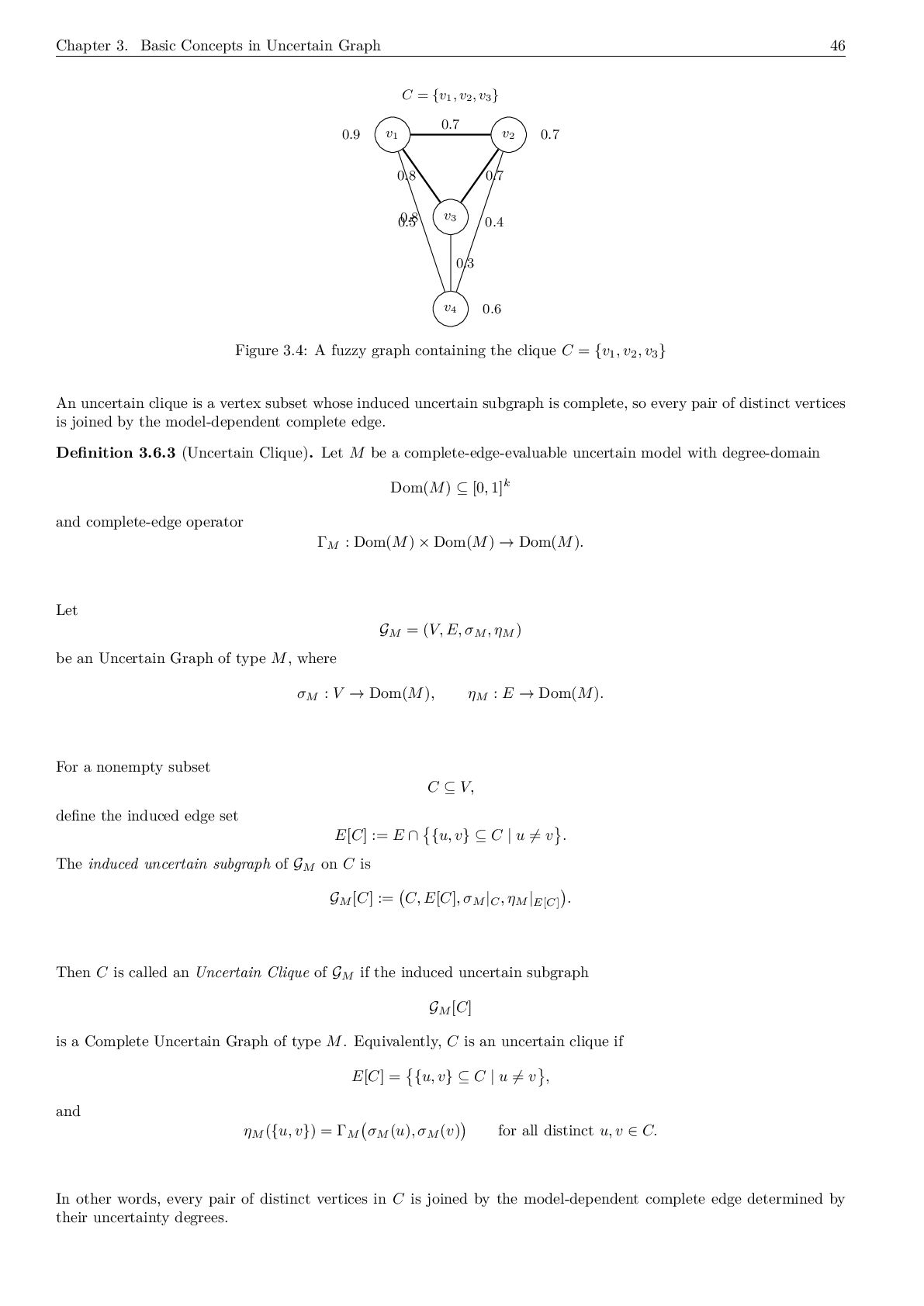
46. 45 Chapter 3. Basic Concepts in Uncertain Graph and the symmetric edge-membership function µ : V × V → [0, 1] given by µ(v1 , v2 ) = 0.7, µ(v1 , v3 ) = 0.8, µ(v2 , v3 ) = 0.7, µ(v1 , v4 ) = 0.5, µ(v2 , v4 ) = 0.4, µ(v3 , v4 ) = 0.3, and µ(vi , vi ) = 0 (i = 1, 2, 3, 4), with µ(u, v) = µ(v, u) (∀ u, v ∈ V ). First, we verify that G is a fuzzy graph. Indeed, µ(v1 , v2 ) = 0.7 = min{0.9, 0.7}, µ(v1 , v3 ) = 0.8 = min{0.9, 0.8}, µ(v2 , v3 ) = 0.7 = min{0.7, 0.8}, µ(v1 , v4 ) = 0.5 ≤ min{0.9, 0.6} = 0.6, µ(v2 , v4 ) = 0.4 ≤ min{0.7, 0.6} = 0.6, and µ(v3 , v4 ) = 0.3 ≤ min{0.8, 0.6} = 0.6. Hence, µ(u, v) ≤ min{σ(u), σ(v)} (∀ u, v ∈ V ). Now consider the subset C = {v1 , v2 , v3 } ⊆ V. Then the induced fuzzy subgraph is G[C] = C, σ|C , µ|C×C . We check the three distinct pairs of vertices in C: µ(v1 , v2 ) = 0.7 = min{σ(v1 ), σ(v2 )}, µ(v1 , v3 ) = 0.8 = min{σ(v1 ), σ(v3 )}, µ(v2 , v3 ) = 0.7 = min{σ(v2 ), σ(v3 )}. Therefore, every pair of distinct vertices in C is adjacent with the maximum possible membership value allowed by their vertex memberships. Hence G[C] is complete, and so C = {v1 , v2 , v3 } is a clique of the fuzzy graph G. On the other hand, the whole vertex set V = {v1 , v2 , v3 , v4 } is not a clique, because for example, µ(v1 , v4 ) = 0.5 < min{0.9, 0.6} = 0.6. Thus, this example shows that a subset of vertices may form a clique even when the entire fuzzy graph is not complete. A schematic illustration is given in Figure 3.4.
47. Chapter 3. Basic Concepts in Uncertain Graph 46 v1 v2 v3 v4 0.7 0.8 0.7 0.5 0.4 0.3 0.9 0.7 0.8 0.6 C = {v1 , v2 , v3 } Figure 3.4: A fuzzy graph containing the clique C = {v1 , v2 , v3 } An uncertain clique is a vertex subset whose induced uncertain subgraph is complete, so every pair of distinct vertices is joined by the model-dependent complete edge. Definition 3.6.3 (Uncertain Clique). Let M be a complete-edge-evaluable uncertain model with degree-domain Dom(M) ⊆ [0, 1]k and complete-edge operator ΓM : Dom(M) × Dom(M) → Dom(M). Let GM = (V, E, σM , ηM ) be an Uncertain Graph of type M, where σM : V → Dom(M), ηM : E → Dom(M). For a nonempty subset C ⊆ V, define the induced edge set E[C] := E ∩ {u, v} ⊆ C | u = v . The induced uncertain subgraph of GM on C is GM [C] := C, E[C], σM |C , ηM |E[C] . Then C is called an Uncertain Clique of GM if the induced uncertain subgraph GM [C] is a Complete Uncertain Graph of type M. Equivalently, C is an uncertain clique if E[C] = {u, v} ⊆ C | u = v , and ηM ({u, v}) = ΓM σM (u), σM (v) for all distinct u, v ∈ C. In other words, every pair of distinct vertices in C is joined by the model-dependent complete edge determined by their uncertainty degrees.
48. 47 Chapter 3. Basic Concepts in Uncertain Graph Theorem 3.6.4 (Well-definedness of Uncertain Clique). Let M be a complete-edge-evaluable uncertain model with degree-domain Dom(M) ⊆ [0, 1]k and symmetric complete-edge operator ΓM : Dom(M) × Dom(M) → Dom(M). Let GM = (V, E, σM , ηM ) be an Uncertain Graph of type M, and let C ⊆ V be a nonempty subset. Then the induced object GM [C] = C, E[C], σM |C , ηM |E[C] is a well-defined Uncertain Graph of type M. Consequently, the statement “C is an Uncertain Clique of GM ” is well-defined. Hence the notion of an uncertain clique is well-defined. Proof. Let C ⊆ V be nonempty. Define E[C] := E ∩ {u, v} ⊆ C | u = v . Since both E and {u, v} ⊆ C | u = v are well-defined sets, the intersection E[C] is well-defined. Because σM : V → Dom(M) is a function, its restriction σM |C : C → Dom(M) is also a well-defined function. Likewise, since ηM : E → Dom(M) is a function and E[C] ⊆ E, the restriction ηM |E[C] : E[C] → Dom(M) is well-defined. Therefore GM [C] = C, E[C], σM |C , ηM |E[C] is a well-defined Uncertain Graph of type M. Now consider the condition that GM [C] be complete. The requirement E[C] = {u, v} ⊆ C | u = v
49. Chapter 3. Basic Concepts in Uncertain Graph 48 is meaningful because both sides are well-defined sets of unordered pairs of vertices. Further, for each distinct u, v ∈ C, the values σM (u), σM (v) ∈ Dom(M) are well-defined, and since ΓM : Dom(M) × Dom(M) → Dom(M) is a well-defined symmetric map, the value ΓM σM (u), σM (v) is well-defined and independent of the order of u and v. Thus the equality ηM ({u, v}) = ΓM σM (u), σM (v) is a meaningful statement for every distinct u, v ∈ C. Hence the predicate GM [C] is a Complete Uncertain Graph is well-defined. By definition, this is exactly the predicate C is an Uncertain Clique of GM . Therefore the notion of uncertain clique is well-defined. For convenience, Table 3.2 summarizes representative clique-related concepts according to the dimension k of the information associated with vertices and/or edges. Table 3.2: Representative clique-related concepts under uncertainty-aware graph frameworks, classified by the dimen- sion k of the information attached to vertices and/or edges. k Clique-related concept Typical coordinate form Canonical information attached to ver- tices/edges 1 Fuzzy Clique µ A clique is studied in a fuzzy graph, where each ver- tex and edge is associated with a single membership degree in [0, 1]. 2 Intuitionistic Fuzzy Clique [182] (µ, ν) A clique is defined in an intuitionistic fuzzy graph, where each vertex and edge carries a membership degree and a non-membership degree, usually satis- fying µ + ν ≤ 1. 3 Neutrosophic Clique (T, I, F) A clique is defined in a neutrosophic graph, where each vertex and edge is described by truth, indeter- minacy, and falsity degrees. Related concepts such as biclique [183, 184], hyperclique [185, 186], quasi-clique [187, 188], k-core [189], k-plex [190], and k-club [191] are also well known. 3.7 Uncertain Star A fuzzy star is a fuzzy graph whose support has one central vertex adjacent to all leaves, while no positive edges exist between leaves pairwise [192–194].
50. 49 Chapter 3. Basic Concepts in Uncertain Graph Definition 3.7.1 (Fuzzy Star). [192,193] Let G = (V, σ, µ) be a finite fuzzy graph, where σ : V → [0, 1], µ : V × V → [0, 1], µ(u, v) ≤ min{σ(u), σ(v)} (∀ u, v ∈ V ), and assume that µ is symmetric and G has no loops. Define the support vertex set and support edge set by V ∗ := {v ∈ V : σ(v) > 0}, E∗ := {u, v} ⊆ V ∗ : u = v, µ(u, v) > 0 . Then G is called a fuzzy star if there exist a vertex c ∈ V ∗ and distinct vertices u1 , u2 , . . . , un ∈ V ∗ (n ≥ 1) such that V ∗ = {c, u1 , u2 , . . . , un }, and E∗ = {c, ui } : 1 ≤ i ≤ n . Equivalently, µ(c, ui ) > 0 (1 ≤ i ≤ n), and µ(ui , uj ) = 0 (1 ≤ i < j ≤ n). In this case, c is called the center of the fuzzy star, the vertices u1 , . . . , un are called its leaves, and the fuzzy star is denoted by S1,n . Example 3.7.2 (Fuzzy star). Let V = {c, u1 , u2 , u3 , u4 }. Define a fuzzy graph G = (V, σ, µ) by the vertex-membership function σ(c) = 0.9, σ(u1 ) = 0.7, σ(u2 ) = 0.6, σ(u3 ) = 0.8, σ(u4 ) = 0.5, and the symmetric edge-membership function µ : V × V → [0, 1] given by µ(c, u1 ) = 0.6, µ(c, u2 ) = 0.5, µ(c, u3 ) = 0.7, µ(c, u4 ) = 0.4, µ(ui , uj ) = 0 (1 ≤ i < j ≤ 4), µ(v, v) = 0 (∀ v ∈ V ), and µ(u, v) = µ(v, u) (∀ u, v ∈ V ). First, we verify that G is a fuzzy graph. Indeed, µ(c, u1 ) = 0.6 ≤ min{σ(c), σ(u1 )} = min{0.9, 0.7} = 0.7, µ(c, u2 ) = 0.5 ≤ min{σ(c), σ(u2 )} = min{0.9, 0.6} = 0.6,
51. Chapter 3. Basic Concepts in Uncertain Graph 50 µ(c, u3 ) = 0.7 ≤ min{σ(c), σ(u3 )} = min{0.9, 0.8} = 0.8, and µ(c, u4 ) = 0.4 ≤ min{σ(c), σ(u4 )} = min{0.9, 0.5} = 0.5. All remaining pairs of distinct leaves have edge-membership value 0, so the condition µ(u, v) ≤ min{σ(u), σ(v)} (∀ u, v ∈ V ) is satisfied. Since all vertex-membership values are positive, the support vertex set is V ∗ = {c, u1 , u2 , u3 , u4 }. Moreover, the only pairs with positive edge-membership are {c, u1 }, {c, u2 }, {c, u3 }, {c, u4 }. Hence the support edge set is E∗ = {c, u1 }, {c, u2 }, {c, u3 }, {c, u4 } . Therefore, V ∗ = {c, u1 , u2 , u3 , u4 }, and E∗ = {c, ui } : 1 ≤ i ≤ 4 . Thus G is a fuzzy star. Its center is c, its leaves are u1 , u2 , u3 , u4 , and the support graph is the star S1,4 . A schematic illustration of this fuzzy star is shown in Figure 3.5. c u1 u2 u3 u4 0.6 0.5 0.7 0.4 0.9 0.7 0.6 0.8 0.5 Figure 3.5: A fuzzy star with center c and leaves u1 , u2 , u3 , u4 An uncertain star is an uncertain graph whose support graph has one central vertex adjacent to all support leaves, while no support edge joins two distinct leaves.
52. 51 Chapter 3. Basic Concepts in Uncertain Graph Definition 3.7.3 (Support-Evaluable Uncertain Model). Let M be an uncertain model with degree-domain Dom(M) ⊆ [0, 1]k. We say that M is support-evaluable if it is equipped with a distinguished element 0M ∈ Dom(M), called the zero degree. Definition 3.7.4 (Uncertain Star). Let M be a support-evaluable uncertain model with degree-domain Dom(M) ⊆ [0, 1]k and zero degree 0M ∈ Dom(M). Let GM = (V, E, σM , ηM ) be an Uncertain Graph of type M, where σM : V → Dom(M), ηM : E → Dom(M). Define the support vertex set and support edge set by V ∗(GM ) := { v ∈ V | σM (v) = 0M }, and E∗(GM ) := { e ∈ E | ηM (e) = 0M }. The support graph of GM is G∗ supp (GM ) := V ∗(GM ), E∗(GM ) . Then GM is called an Uncertain Star if there exist a vertex c ∈ V ∗(GM ) and distinct vertices u1 , u2 , . . . , un ∈ V ∗(GM ) (n ≥ 1) such that V ∗(GM ) = {c, u1 , u2 , . . . , un }, and E∗(GM ) = {c, ui } | 1 ≤ i ≤ n . Equivalently, the support graph G∗ supp (GM ) is isomorphic to the star graph K1,n . In this case, c is called a center of the uncertain star and u1 , . . . , un are called its leaves.
53. Chapter 3. Basic Concepts in Uncertain Graph 52 Theorem 3.7.5 (Well-definedness of Uncertain Star). Let M be a support-evaluable uncertain model with degree- domain Dom(M) ⊆ [0, 1]k and zero degree 0M ∈ Dom(M). Let GM = (V, E, σM , ηM ) be an Uncertain Graph of type M. Then the support sets V ∗(GM ) = { v ∈ V | σM (v) = 0M } and E∗(GM ) = { e ∈ E | ηM (e) = 0M } are well-defined. Consequently, the support graph G∗ supp (GM ) = V ∗(GM ), E∗(GM ) is well-defined, and the statement “GM is an Uncertain Star” is well-defined. Hence the notion of an uncertain star is well-defined. Proof. Since M is an uncertain model, its degree-domain Dom(M) is fixed. Since M is support-evaluable, the element 0M ∈ Dom(M) is also fixed. Because σM : V → Dom(M) is a function, for each v ∈ V the value σM (v) is uniquely determined in Dom(M). Therefore the condition σM (v) = 0M is meaningful for every v ∈ V . Hence V ∗(GM ) = { v ∈ V | σM (v) = 0M } is a well-defined subset of V . Likewise, since ηM : E → Dom(M) is a function, for each e ∈ E the value ηM (e) is uniquely determined in Dom(M). Therefore the condition ηM (e) = 0M
54. 53 Chapter 3. Basic Concepts in Uncertain Graph is meaningful for every e ∈ E. Hence E∗(GM ) = { e ∈ E | ηM (e) = 0M } is a well-defined subset of E. Thus the pair G∗ supp (GM ) = V ∗(GM ), E∗(GM ) is a well-defined graph. Now the condition that GM be an uncertain star asserts the existence of a vertex c ∈ V ∗(GM ) and distinct vertices u1 , . . . , un ∈ V ∗(GM ) such that V ∗(GM ) = {c, u1 , . . . , un } and E∗(GM ) = {c, ui } | 1 ≤ i ≤ n . Since both V ∗(GM ) and E∗(GM ) are already well-defined, these set equalities are meaningful statements. Equivalently, the condition that G∗ supp (GM ) ∼ = K1,n is also meaningful, because both graphs are well-defined crisp graphs. Therefore the predicate “GM is an Uncertain Star” is well-defined. Hence the notion of an uncertain star is well-defined. For convenience, Table 3.3 summarizes representative star-related concepts according to the dimension k of the information associated with vertices and/or edges. Related concepts other than the uncertain star are also known, such as the double star [198–200], subdivided star [201,202], spider graph [203], and directed star [204,205]. 3.8 Uncertain Radius and Diameter The radius of a fuzzy graph is the minimum eccentricity among its vertices, measuring how close the most central vertex is to all others overall (cf. [206]). The diameter of a fuzzy graph is the maximum eccentricity among its vertices, measuring the greatest distance from a vertex to any other vertex overall(cf. [206]).
55. Chapter 3. Basic Concepts in Uncertain Graph 54 Table 3.3: Representative star-related concepts under uncertainty-aware graph frameworks, classified by the dimension k of the information attached to vertices and/or edges. k Star-related concept Typical coordinate form Canonical information attached to ver- tices/edges 1 Fuzzy Star µ A star is studied in a fuzzy graph, where each ver- tex and edge is associated with a single member- ship degree in [0, 1]. 2 Intuitionistic Fuzzy Star [195] (µ, ν) A star is defined in an intuitionistic fuzzy graph, where each vertex and edge carries a membership degree and a non-membership degree, usually sat- isfying µ + ν ≤ 1. 3 Neutrosophic Star [196] (T, I, F) A star is defined in a neutrosophic graph, where each vertex and edge is described by truth, inde- terminacy, and falsity degrees. s + t Plithogenic Star [197] (a, c) ∈ [0, 1]s × [0, 1]t A star is defined in a plithogenic graph, where each vertex and edge is described by attribute-based in- formation together with an s-dimensional appur- tenance vector and a t-dimensional contradiction vector. Definition 3.8.1 (Radius and Diameter in a Fuzzy Graph). Let G = (V, σ, µ) be a finite connected fuzzy graph, and let dµ : V × V → [0, ∞) be the fuzzy distance on G, defined by dµ (u, v) := min µ (P) : P is a path from u to v , where, for a path P : u0 , u1 , . . . , un , its µ-length is µ (P) := n i=1 1 µ(ui−1 , ui ) . For each vertex v ∈ V , the eccentricity of v is defined by eµ (v) := max u∈V dµ (v, u). The radius of the fuzzy graph G is defined by rµ (G) := min v∈V eµ (v), and the diameter of the fuzzy graph G is defined by dµ (G) := max v∈V eµ (v). Example 3.8.2 (Radius and diameter in a fuzzy graph). Let V = {v1 , v2 , v3 , v4 }. Define a fuzzy graph G = (V, σ, µ)
56. 55 Chapter 3. Basic Concepts in Uncertain Graph by the vertex-membership function σ(v1 ) = 0.9, σ(v2 ) = 0.8, σ(v3 ) = 0.8, σ(v4 ) = 0.9, and the symmetric edge-membership function µ : V × V → [0, 1] given by µ(v1 , v2 ) = 0.8, µ(v2 , v3 ) = 0.5, µ(v3 , v4 ) = 0.8, and µ(u, v) = 0 for all other unordered pairs {u, v} ⊆ V , with µ(u, v) = µ(v, u) (∀ u, v ∈ V ). First, we verify that G is a fuzzy graph. Indeed, µ(v1 , v2 ) = 0.8 ≤ min{0.9, 0.8} = 0.8, µ(v2 , v3 ) = 0.5 ≤ min{0.8, 0.8} = 0.8, and µ(v3 , v4 ) = 0.8 ≤ min{0.8, 0.9} = 0.8. Hence µ(u, v) ≤ min{σ(u), σ(v)} (∀ u, v ∈ V ). Since the positive edges are exactly {v1 , v2 }, {v2 , v3 }, {v3 , v4 }, the support graph is the path v1 − v2 − v3 − v4 , which is connected. Therefore the fuzzy distance dµ is well defined for every pair of vertices. Because the support graph is a path, each pair of vertices is joined by a unique path. Thus the fuzzy distances are obtained by summing reciprocals of the corresponding edge-membership values. We have dµ (v1 , v2 ) = 1 0.8 = 5 4 , dµ (v2 , v3 ) = 1 0.5 = 2, dµ (v3 , v4 ) = 1 0.8 = 5 4 . Also, dµ (v1 , v3 ) = 1 0.8 + 1 0.5 = 5 4 + 2 = 13 4 , dµ (v2 , v4 ) = 1 0.5 + 1 0.8 = 2 + 5 4 = 13 4 , and dµ (v1 , v4 ) = 1 0.8 + 1 0.5 + 1 0.8 = 5 4 + 2 + 5 4 = 9 2 . Of course, dµ (vi , vi ) = 0 (i = 1, 2, 3, 4). Hence the eccentricity of each vertex is eµ (v1 ) = max 0, 5 4 , 13 4 , 9 2 = 9 2 ,
57. Chapter 3. Basic Concepts in Uncertain Graph 56 eµ (v2 ) = max 5 4 , 0, 2, 13 4 = 13 4 , eµ (v3 ) = max 13 4 , 2, 0, 5 4 = 13 4 , eµ (v4 ) = max 9 2 , 13 4 , 5 4 , 0 = 9 2 . Therefore the radius of G is rµ (G) = min v∈V eµ (v) = min 9 2 , 13 4 , 13 4 , 9 2 = 13 4 , and the diameter of G is dµ (G) = max v∈V eµ (v) = max 9 2 , 13 4 , 13 4 , 9 2 = 9 2 . Thus the vertices v2 and v3 are the central vertices of this fuzzy graph, while the largest fuzzy distance occurs between the end vertices v1 and v4 . A schematic illustration of this fuzzy graph is shown in Figure 3.6. v1 v2 v3 v4 0.8 0.5 0.8 σ(v1 ) = 0.9 σ(v2 ) = 0.8 σ(v3 ) = 0.8 σ(v4 ) = 0.9 eµ (v2 ) = 13 4 eµ (v3 ) = 13 4 Figure 3.6: A fuzzy graph illustrating radius and diameter The radius of an uncertain graph is the minimum eccentricity among its vertices, while the diameter is the maximum eccentricity among its vertices. Definition 3.8.3 (Uncertain Radius and Diameter). Let GM = (V, E, σM , ηM ) be a finite connected Uncertain Graph of type M, and let dM : V × V → [0, ∞) be the uncertain distance on GM . For each vertex v ∈ V , the uncertain eccentricity of v is defined by eM (v) := max u∈V dM (v, u). The uncertain radius of GM is defined by rM (GM ) := min v∈V eM (v), and the uncertain diameter of GM is defined by DM (GM ) := max v∈V eM (v).
58. 57 Chapter 3. Basic Concepts in Uncertain Graph Theorem 3.8.4 (Well-definedness of Uncertain Radius and Diameter). Let GM = (V, E, σM , ηM ) be a finite connected Uncertain Graph of type M, and suppose that the uncertain distance dM : V × V → [0, ∞) is well-defined. Then: 1. for every vertex v ∈ V , the uncertain eccentricity eM (v) = max u∈V dM (v, u) is well-defined; 2. the uncertain radius rM (GM ) = min v∈V eM (v) is well-defined; 3. the uncertain diameter DM (GM ) = max v∈V eM (v) is well-defined. Hence the notions of uncertain eccentricity, uncertain radius, and uncertain diameter are well-defined. Proof. Since GM is finite, the vertex set V is a finite nonempty set. Fix a vertex v ∈ V . Because the uncertain distance dM : V × V → [0, ∞) is well-defined, the value dM (v, u) ∈ [0, ∞) is well-defined for every u ∈ V . Therefore the set { dM (v, u) | u ∈ V } is a finite nonempty subset of [0, ∞). Every finite nonempty subset of R has a maximum, so eM (v) := max u∈V dM (v, u) exists and is uniquely determined. Hence the uncertain eccentricity of v is well-defined. Now consider the set of all vertex eccentricities: { eM (v) | v ∈ V }. Since V is finite and nonempty, this is again a finite nonempty subset of [0, ∞). Therefore it has both a minimum and a maximum. Consequently, rM (GM ) := min v∈V eM (v) and DM (GM ) := max v∈V eM (v) exist and are uniquely determined. Thus uncertain eccentricity, uncertain radius, and uncertain diameter are all well-defined.
59. Chapter 3. Basic Concepts in Uncertain Graph 58 3.9 Uncertain Wheel A fuzzy wheel is a fuzzy graph whose support is a wheel, with one central hub joined to all vertices of an outer cycle [170,207,208]. Definition 3.9.1 (Fuzzy Wheel). Let G = (V, σ, µ) be a finite fuzzy graph, where σ : V → [0, 1], µ : V × V → [0, 1], µ(u, v) ≤ min{σ(u), σ(v)} (∀ u, v ∈ V ), and assume that µ is symmetric and G has no loops. Define the support vertex set and support edge set by V ∗ := {v ∈ V : σ(v) > 0}, E∗ := {u, v} ⊆ V ∗ : u = v, µ(u, v) > 0 . Then G is called a fuzzy wheel if there exist a vertex c ∈ V ∗ and distinct vertices v1 , v2 , . . . , vn ∈ V ∗ (n ≥ 3) such that V ∗ = {c, v1 , v2 , . . . , vn }, and E∗ = {vi , vi+1 } : 1 ≤ i ≤ n − 1 ∪ {vn , v1 } ∪ {c, vi } : 1 ≤ i ≤ n . Equivalently, the support graph G∗ = (V ∗, E∗) is isomorphic to the wheel graph Wn+1 = K1 + Cn . In this case, c is called the hub (or center) of the fuzzy wheel, and v1 , v2 , . . . , vn form its outer fuzzy cycle. Example 3.9.2 (Fuzzy wheel). Let V = {c, v1 , v2 , v3 , v4 , v5 }. Define a fuzzy graph G = (V, σ, µ) by the vertex-membership function σ(c) = 0.9, σ(v1 ) = 0.8, σ(v2 ) = 0.7, σ(v3 ) = 0.8, σ(v4 ) = 0.6, σ(v5 ) = 0.7, and the symmetric edge-membership function µ : V × V → [0, 1] given by µ(v1 , v2 ) = 0.6, µ(v2 , v3 ) = 0.6, µ(v3 , v4 ) = 0.5, µ(v4 , v5 ) = 0.5, µ(v5 , v1 ) = 0.6, µ(c, v1 ) = 0.7, µ(c, v2 ) = 0.6, µ(c, v3 ) = 0.7, µ(c, v4 ) = 0.5, µ(c, v5 ) = 0.6, µ(v, v) = 0 (∀ v ∈ V ), and µ(u, v) = 0
60. 59 Chapter 3. Basic Concepts in Uncertain Graph for all other distinct pairs {u, v} ⊆ V , with µ(u, v) = µ(v, u) (∀ u, v ∈ V ). First, we verify that G is a fuzzy graph. Indeed, µ(v1 , v2 ) = 0.6 ≤ min{0.8, 0.7} = 0.7, µ(v2 , v3 ) = 0.6 ≤ min{0.7, 0.8} = 0.7, µ(v3 , v4 ) = 0.5 ≤ min{0.8, 0.6} = 0.6, µ(v4 , v5 ) = 0.5 ≤ min{0.6, 0.7} = 0.6, µ(v5 , v1 ) = 0.6 ≤ min{0.7, 0.8} = 0.7, and µ(c, v1 ) = 0.7 ≤ min{0.9, 0.8} = 0.8, µ(c, v2 ) = 0.6 ≤ min{0.9, 0.7} = 0.7, µ(c, v3 ) = 0.7 ≤ min{0.9, 0.8} = 0.8, µ(c, v4 ) = 0.5 ≤ min{0.9, 0.6} = 0.6, µ(c, v5 ) = 0.6 ≤ min{0.9, 0.7} = 0.7. Hence µ(u, v) ≤ min{σ(u), σ(v)} (∀ u, v ∈ V ). Since all vertex-membership values are positive, the support vertex set is V ∗ = {c, v1 , v2 , v3 , v4 , v5 }. Moreover, the positive edges are exactly {v1 , v2 }, {v2 , v3 }, {v3 , v4 }, {v4 , v5 }, {v5 , v1 }, together with {c, v1 }, {c, v2 }, {c, v3 }, {c, v4 }, {c, v5 }. Therefore, E∗ = {vi , vi+1 } : 1 ≤ i ≤ 4 ∪ {v5 , v1 } ∪ {c, vi } : 1 ≤ i ≤ 5 . Thus the support graph is a wheel: G∗ ∼ = W6 = K1 + C5 . Hence G is a fuzzy wheel with hub c, and v1 , v2 , v3 , v4 , v5 form its outer fuzzy cycle. A schematic illustration of this fuzzy wheel is shown in Figure 3.7. An uncertain wheel is an uncertain graph whose support graph is a wheel, consisting of one hub adjacent to every vertex of an outer cycle. Definition 3.9.3 (Support-Evaluable Uncertain Model). Let M be an uncertain model with degree-domain Dom(M) ⊆ [0, 1]k. We say that M is support-evaluable if it is equipped with a distinguished element 0M ∈ Dom(M), called the zero degree.
61. Chapter 3. Basic Concepts in Uncertain Graph 60 c v1 v2 v3 v4 v5 0.6 0.6 0.5 0.5 0.6 0.7 0.6 0.7 0.5 0.6 0.8 0.7 0.8 0.6 0.7 0.9 Figure 3.7: A fuzzy wheel with hub c and outer fuzzy cycle v1 v2 v3 v4 v5 v1 Definition 3.9.4 (Uncertain Wheel). Let M be a support-evaluable uncertain model with degree-domain Dom(M) ⊆ [0, 1]k and zero degree 0M ∈ Dom(M). Let GM = (V, E, σM , ηM ) be an Uncertain Graph of type M, where σM : V → Dom(M), ηM : E → Dom(M). Define the support vertex set by V ∗(GM ) := { v ∈ V | σM (v) = 0M }, and define the support edge set by E∗(GM ) := {u, v} ∈ E | u, v ∈ V ∗(GM ), ηM ({u, v}) = 0M . The support graph of GM is G∗ supp (GM ) := V ∗(GM ), E∗(GM ) . Then GM is called an Uncertain Wheel if there exist a vertex c ∈ V ∗(GM ) and distinct vertices v1 , v2 , . . . , vn ∈ V ∗(GM ) (n ≥ 3) such that V ∗(GM ) = {c, v1 , v2 , . . . , vn }, and E∗(GM ) = {vi , vi+1 } : 1 ≤ i ≤ n − 1 ∪ {vn , v1 } ∪ {c, vi } : 1 ≤ i ≤ n . Equivalently, GM is an uncertain wheel if its support graph is isomorphic to the wheel graph Wn+1 = K1 + Cn . In this case, c is called the hub (or center) of the uncertain wheel, and v1 , v2 , . . . , vn form its outer cycle.
62. 61 Chapter 3. Basic Concepts in Uncertain Graph Theorem 3.9.5 (Well-definedness of Uncertain Wheel). Let M be a support-evaluable uncertain model with degree- domain Dom(M) ⊆ [0, 1]k and zero degree 0M ∈ Dom(M). Let GM = (V, E, σM , ηM ) be an Uncertain Graph of type M. Then the support sets V ∗(GM ) = { v ∈ V | σM (v) = 0M } and E∗(GM ) = {u, v} ∈ E | u, v ∈ V ∗(GM ), ηM ({u, v}) = 0M are well-defined. Consequently, the support graph G∗ supp (GM ) = V ∗(GM ), E∗(GM ) is well-defined, and the statement “GM is an Uncertain Wheel” is well-defined. Hence the notion of an uncertain wheel is well-defined. Proof. Since M is an uncertain model, its degree-domain Dom(M) is fixed. Since M is support-evaluable, the element 0M ∈ Dom(M) is fixed as well. Because σM : V → Dom(M) is a function, for each v ∈ V the value σM (v) is uniquely determined in Dom(M). Hence the condition σM (v) = 0M is meaningful for every v ∈ V . Therefore V ∗(GM ) = { v ∈ V | σM (v) = 0M } is a well-defined subset of V . Likewise, because ηM : E → Dom(M) is a function, for each edge e ∈ E the value ηM (e) is uniquely determined in Dom(M). Hence the condition ηM (e) = 0M
63. Chapter 3. Basic Concepts in Uncertain Graph 62 is meaningful for every e ∈ E. Now define E∗(GM ) = {u, v} ∈ E | u, v ∈ V ∗(GM ), ηM ({u, v}) = 0M . Since E and V ∗(GM ) are well-defined, and since the predicate u, v ∈ V ∗(GM ), ηM ({u, v}) = 0M is meaningful, the set E∗(GM ) is a well-defined subset of E. Therefore the pair G∗ supp (GM ) = V ∗(GM ), E∗(GM ) is a well-defined graph. The statement that GM is an uncertain wheel asserts that there exist a vertex c ∈ V ∗(GM ) and distinct vertices v1 , . . . , vn ∈ V ∗(GM ) (n ≥ 3) such that V ∗(GM ) = {c, v1 , . . . , vn }, and E∗(GM ) = {vi , vi+1 } : 1 ≤ i ≤ n − 1 ∪ {vn , v1 } ∪ {c, vi } : 1 ≤ i ≤ n . Since both V ∗(GM ) and E∗(GM ) are well-defined sets, these equalities are meaningful. Equivalently, the statement G∗ supp (GM ) ∼ = Wn+1 is meaningful because both graphs are well-defined crisp graphs. Hence the predicate “GM is an Uncertain Wheel” is well-defined. Therefore the notion of an uncertain wheel is well-defined. Representative wheel-related concepts under uncertainty-aware graph frameworks are listed in Table 3.4. Related concepts such as the gear graph [212,213], helm graph [214], fan graph [215], friendship graph [216], multi- wheel graph [217,218], and double wheel graph [219] are also well known.
64. 63 Chapter 3. Basic Concepts in Uncertain Graph Table 3.4: Representative wheel-related concepts under uncertainty-aware graph frameworks, classified by the dimen- sion k of the information attached to vertices and/or edges. k Wheel-related concept Typical coordinate form Canonical information attached to ver- tices/edges 1 Fuzzy Wheel µ A wheel is studied in a fuzzy graph, where each ver- tex and edge is associated with a single membership degree in [0, 1]. 2 Intuitionistic Fuzzy Wheel [209,210] (µ, ν) A wheel is defined in an intuitionistic fuzzy graph, where each vertex and edge carries a membership degree and a non-membership degree, usually satis- fying µ + ν ≤ 1. 3 Neutrosophic Wheel [211] (T, I, F) A wheel is defined in a neutrosophic graph, where each vertex and edge is described by truth, indeter- minacy, and falsity degrees.
65. Chapter 3. Basic Concepts in Uncertain Graph 64
66. Chapter 4 Graph Classes In this chapter, graph classes based on fuzzy graphs and uncertain graphs are introduced and investigated. 4.1 Uncertain Digraph A fuzzy directed graph assigns membership values to vertices and directed edges [220–223]. Definition 4.1.1 (Fuzzy Directed Graph). [224–226] A fuzzy directed graph is a quadruple G = (V, E, σ, µ), where • V is a nonempty set of vertices, • E ⊆ V × V is a set of directed edges, • σ : V → [0, 1] assigns a membership degree to each vertex, • µ : E → [0, 1] assigns a membership degree to each directed edge, such that, for every (u, v) ∈ E, µ(u, v) ≤ min{σ(u), σ(v)}. Example 4.1.2 (Fuzzy directed graph). Let V = {v1 , v2 , v3 , v4 }, and define the directed edge set by E = {(v1 , v2 ), (v2 , v3 ), (v3 , v1 ), (v1 , v4 ), (v4 , v3 )}. Define the vertex-membership function σ : V → [0, 1] by σ(v1 ) = 0.9, σ(v2 ) = 0.7, σ(v3 ) = 0.8, σ(v4 ) = 0.6, 65
67. Chapter 4. Graph Classes 66 and define the directed edge-membership function µ : E → [0, 1] by µ(v1 , v2 ) = 0.6, µ(v2 , v3 ) = 0.5, µ(v3 , v1 ) = 0.7, µ(v1 , v4 ) = 0.4, µ(v4 , v3 ) = 0.5. Then G = (V, E, σ, µ) is a fuzzy directed graph, because for every directed edge (u, v) ∈ E, µ(u, v) ≤ min{σ(u), σ(v)}. Indeed, µ(v1 , v2 ) = 0.6 ≤ min{0.9, 0.7} = 0.7, µ(v2 , v3 ) = 0.5 ≤ min{0.7, 0.8} = 0.7, µ(v3 , v1 ) = 0.7 ≤ min{0.8, 0.9} = 0.8, µ(v1 , v4 ) = 0.4 ≤ min{0.9, 0.6} = 0.6, and µ(v4 , v3 ) = 0.5 ≤ min{0.6, 0.8} = 0.6. Hence all required conditions are satisfied. Observe that this graph is genuinely directed. For example, (v1 , v2 ) ∈ E, but (v2 , v1 ) / ∈ E, so the edge relation is not symmetric. A schematic illustration of this fuzzy directed graph is shown in Figure 4.1. v1 v2 v3 v4 0.6 0.5 0.7 0.4 0.5 0.9 0.7 0.8 0.6 Figure 4.1: A fuzzy directed graph An uncertain directed graph assigns uncertainty degrees to vertices and directed edges, thereby representing asym- metric uncertain relations among vertices. Definition 4.1.3 (Uncertain Directed Graph). Let D∗ = (V, A) be a finite directed graph, where A ⊆ V × V
68. 67 Chapter 4. Graph Classes is the set of directed edges (arcs). Assume that D∗ is loopless, that is, (u, u) / ∈ A (∀ u ∈ V ). Let M be a fixed uncertain model with degree-domain Dom(M) ⊆ [0, 1]k. An Uncertain Directed Graph of type M is a quadruple DM = (V, A, σM , αM ), where σM : V −→ Dom(M) and αM : A −→ Dom(M) are uncertainty-degree functions on the vertex set and the arc set, respectively. Equivalently, (V, σM ) is an Uncertain Set of type M on V , and (A, αM ) is an Uncertain Set of type M on A. For each vertex v ∈ V , the value σM (v) ∈ Dom(M) represents the uncertainty degree of v, and for each arc (u, v) ∈ A, the value αM ((u, v)) ∈ Dom(M) represents the uncertainty degree of the directed edge from u to v. If desired, one may additionally impose model-specific compatibility conditions involving σM (u), σM (v), αM ((u, v)), but such conditions depend on the chosen uncertain model M and are not fixed at the level of this general definition. Theorem 4.1.4 (Well-definedness of Uncertain Directed Graph). Let D∗ = (V, A) be a finite loopless directed graph, let M be an uncertain model with degree-domain Dom(M) ⊆ [0, 1]k, and let σM : V → Dom(M), αM : A → Dom(M) be functions. Then DM = (V, A, σM , αM )
69. Chapter 4. Graph Classes 68 is a well-defined Uncertain Directed Graph of type M. Moreover, (V, σM ) is an Uncertain Set of type M on V , and (A, αM ) is an Uncertain Set of type M on A. Proof. Since M is an uncertain model, its degree-domain Dom(M) is fixed. Hence the maps σM : V → Dom(M) and αM : A → Dom(M) are ordinary set-theoretic functions with well-specified codomain Dom(M). Therefore the pairs (V, σM ) and (A, αM ) are Uncertain Sets of type M on V and A, respectively. Next, because A ⊆ V × V, every arc a ∈ A is a uniquely determined ordered pair a = (u, v) with u, v ∈ V . Hence each directed edge has a uniquely determined source u and a uniquely determined target v. Accordingly, for every arc (u, v) ∈ A, the value αM ((u, v)) ∈ Dom(M) is unambiguously assigned to that ordered pair. Since order matters in V × V , the arcs (u, v) and (v, u) are distinct whenever u = v, so no ambiguity arises between opposite directions. Thus all components of DM = (V, A, σM , αM ) are simultaneously and uniquely specified: • V is the vertex set; • A is the arc set; • σM assigns a unique uncertainty degree to each vertex; • αM assigns a unique uncertainty degree to each directed edge. Hence DM = (V, A, σM , αM ) defines a unique mathematical object, namely an Uncertain Directed Graph of type M. Therefore the definition is well-defined. Representative directed-graph concepts under uncertainty-aware graph frameworks are listed in Table 4.1.
70. 69 Chapter 4. Graph Classes Table 4.1: Representative directed-graph concepts under uncertainty-aware graph frameworks, classified by the di- mension k of the information attached to vertices and/or edges. k Directed-graph concept Typical coordinate form Canonical information attached to ver- tices/edges 1 Fuzzy Directed Graph [227–229] µ A directed graph in which each vertex and arc is associated with a single membership degree in [0, 1]. 2 Vague Directed Graph [230,231] (t, f) A directed graph in which each vertex and arc is described by a truth-membership degree and a falsity-membership degree, typically with t+f ≤ 1. 2 Intuitionistic Fuzzy Directed Graph [232–234] (µ, ν) A directed graph in which each vertex and arc carries a membership degree and a non- membership degree, usually satisfying µ + ν ≤ 1. 3 Spherical Fuzzy Directed Graph [235] (µ, η, ν) A directed graph in which each vertex and arc is assigned positive, neutral, and negative member- ship degrees, usually satisfying µ2 + η2 + ν2 ≤ 1. 3 Picture Fuzzy Digraph [236,237] (µ, η, ν) A directed graph in which each vertex and arc is described by positive, neutral, and negative membership degrees, usually satisfying µ+η+ν ≤ 1. 3 Neutrosophic Directed Graph [131,238,239] (T, I, F) A directed graph in which each vertex and arc is described by truth, indeterminacy, and falsity degrees. s + t Plithogenic Directed Graph [240] (a, c) ∈ [0, 1]s × [0, 1]t A directed graph in which each vertex and arc is described by attribute-based information to- gether with an s-dimensional appurtenance vec- tor and a t-dimensional contradiction vector. 4.2 Uncertain Bidirected Graph A fuzzy bidirected graph assigns membership values to vertices and edges, while each endpoint of an edge has its own local orientation [241]. Definition 4.2.1 (Fuzzy Bidirected Graph). [241] A fuzzy bidirected graph is a quintuple G = (V, E, σ, µ, τ), where • V is a nonempty set of vertices, • E ⊆ {u, v} | u, v ∈ V, u = v is a set of bidirected edges, • σ : V → [0, 1] assigns a membership degree to each vertex, • µ : E → [0, 1] assigns a membership degree to each edge, • τ : V × E → {−1, 0, 1} is a bidirection function, such that, for each edge e = {u, v} ∈ E, τ(u, e), τ(v, e) ∈ {−1, 1}, τ(w, e) = 0 for all w ∈ V \ {u, v}, and µ(e) ≤ min{σ(u), σ(v)}. Thus each endpoint of a fuzzy edge carries its own local orientation.
71. Chapter 4. Graph Classes 70 Example 4.2.2 (Fuzzy bidirected graph). Let V = {v1 , v2 , v3 , v4 }, and let E = {e12 , e23 , e13 , e34 }, where e12 = {v1 , v2 }, e23 = {v2 , v3 }, e13 = {v1 , v3 }, e34 = {v3 , v4 }. Define the vertex-membership function σ : V → [0, 1] by σ(v1 ) = 0.9, σ(v2 ) = 0.8, σ(v3 ) = 0.7, σ(v4 ) = 0.6. Define the edge-membership function µ : E → [0, 1] by µ(e12 ) = 0.6, µ(e23 ) = 0.5, µ(e13 ) = 0.7, µ(e34 ) = 0.4. Next, define the bidirection function τ : V × E → {−1, 0, 1} as follows: τ(v1 , e12 ) = 1, τ(v2 , e12 ) = −1, τ(v2 , e23 ) = 1, τ(v3 , e23 ) = 1, τ(v1 , e13 ) = −1, τ(v3 , e13 ) = 1, τ(v3 , e34 ) = −1, τ(v4 , e34 ) = −1, and τ(w, e) = 0 for every pair (w, e) not listed above. Then G = (V, E, σ, µ, τ) is a fuzzy bidirected graph. Indeed, for each edge e = {u, v} ∈ E, the values at its endpoints belong to {−1, 1}, while every non-incident vertex receives value 0. For example, for the edge e12 = {v1 , v2 }, we have τ(v1 , e12 ) = 1, τ(v2 , e12 ) = −1, and τ(v3 , e12 ) = τ(v4 , e12 ) = 0. Similarly, the same property holds for e23 , e13 , and e34 . Moreover, the membership condition is satisfied: µ(e12 ) = 0.6 ≤ min{σ(v1 ), σ(v2 )} = min{0.9, 0.8} = 0.8,
72. 71 Chapter 4. Graph Classes µ(e23 ) = 0.5 ≤ min{σ(v2 ), σ(v3 )} = min{0.8, 0.7} = 0.7, µ(e13 ) = 0.7 ≤ min{σ(v1 ), σ(v3 )} = min{0.9, 0.7} = 0.7, and µ(e34 ) = 0.4 ≤ min{σ(v3 ), σ(v4 )} = min{0.7, 0.6} = 0.6. Hence all requirements in the definition are fulfilled. Therefore, G = (V, E, σ, µ, τ) is a fuzzy bidirected graph. A schematic illustration is shown in Figure 4.2. In the figure, the number written near the midpoint of each edge is µ(e), while the small signs near the endpoints indicate the corresponding values of τ(·, e). v1 v2 v3 v4 0.6 0.5 0.7 0.4 0.9 0.8 0.7 0.6 +1 −1 +1 +1 −1 +1 −1 −1 Figure 4.2: A fuzzy bidirected graph The extensions based on Uncertain Sets are presented below. Definition 4.2.3 (Uncertain Bidirected Graph). Let B∗ = (V, E, τ) be a finite bidirected graph, where E ⊆ {u, v} | u, v ∈ V, u = v is a set of undirected edges, and τ : V × E → {−1, 0, 1} is a bidirection function satisfying the following condition: for each edge e = {u, v} ∈ E, we have τ(u, e), τ(v, e) ∈ {−1, 1}, τ(w, e) = 0 for all w ∈ V \ {u, v}. Let M be a fixed uncertain model with degree-domain Dom(M) ⊆ [0, 1]k. An Uncertain Bidirected Graph of type M is a quintuple BM = (V, E, τ, σM , ηM ), where σM : V −→ Dom(M) and ηM : E −→ Dom(M)
73. Chapter 4. Graph Classes 72 are uncertainty-degree functions on the vertex set and the edge set, respectively. Equivalently, (V, σM ) is an Uncertain Set of type M on V , and (E, ηM ) is an Uncertain Set of type M on E. For each vertex v ∈ V , the value σM (v) ∈ Dom(M) represents the uncertainty degree of v, and for each edge e ∈ E, the value ηM (e) ∈ Dom(M) represents the uncertainty degree of e, while the function τ assigns an independent local orientation at each endpoint of every edge. If desired, one may additionally impose model-specific compatibility conditions between ηM (e) and the endpoint degrees σM (u), σM (v) for e = {u, v}, but such conditions depend on the chosen uncertain model M and are not fixed at the level of this general definition. Theorem 4.2.4 (Well-definedness of Uncertain Bidirected Graph). Let B∗ = (V, E, τ) be a finite bidirected graph, where E ⊆ {u, v} | u, v ∈ V, u = v and τ : V × E → {−1, 0, 1} satisfies the bidirected-incidence condition: for every edge e = {u, v} ∈ E, there exist exactly two distinct vertices u, v ∈ V such that τ(u, e), τ(v, e) ∈ {−1, 1}, τ(w, e) = 0 for all w ∈ V \ {u, v}. Let M be an uncertain model with degree-domain Dom(M) ⊆ [0, 1]k, and let σM : V → Dom(M), ηM : E → Dom(M) be functions. Then the quintuple BM = (V, E, τ, σM , ηM ) is a well-defined Uncertain Bidirected Graph of type M. Moreover, (V, σM ) is an Uncertain Set of type M on the vertex set V , and (E, ηM ) is an Uncertain Set of type M on the edge set E.
74. 73 Chapter 4. Graph Classes Proof. Since M is an uncertain model, its degree-domain Dom(M) is a fixed admissible set of uncertainty degrees. Hence the maps σM : V → Dom(M) and ηM : E → Dom(M) are ordinary set-theoretic functions with well-specified codomain Dom(M). Therefore the pairs (V, σM ) and (E, ηM ) are Uncertain Sets of type M on V and E, respectively. Next, because B∗ = (V, E, τ) is a bidirected graph, every edge e ∈ E is an unordered two-element subset of V , say e = {u, v}, u = v, and the bidirection function τ assigns local orientations only to the two incidences (u, e) and (v, e), while all nonincident pairs (w, e) have value 0. Thus the local orientation data attached to each edge is unambiguous. Therefore all components of BM = (V, E, τ, σM , ηM ) are simultaneously well specified: • V is the vertex set; • E is the set of bidirected edges; • τ is the bidirection function on incidences; • σM assigns to each vertex a unique uncertainty degree in Dom(M); • ηM assigns to each edge a unique uncertainty degree in Dom(M). Hence the quintuple BM = (V, E, τ, σM , ηM ) defines a unique mathematical object, namely an Uncertain Bidirected Graph of type M. Therefore the definition is well-defined. 4.3 Uncertain MutliDirected Graph A fuzzy multidirected graph assigns membership values to vertices and directed edges and allows multiple parallel directed edges between the same ordered pair [241]. Definition 4.3.1 (Fuzzy MultiDirected Graph). A fuzzy multidirected graph is a quadruple G = (V, E, σ, µ), where • V is a nonempty set of vertices, • E is a multiset of directed edges, each edge e ∈ E being an ordered pair e = (u, v) ∈ V × V, so that multiple parallel directed edges between the same ordered pair are allowed,
75. Chapter 4. Graph Classes 74 • σ : V → [0, 1] assigns a membership degree to each vertex, • µ : E → [0, 1] assigns a membership degree to each directed edge, such that, for every edge e = (u, v) ∈ E, µ(e) ≤ min{σ(u), σ(v)}. Equivalently, if s, t : E → V denote the source and target maps, then µ(e) ≤ min{σ(s(e)), σ(t(e))} (∀e ∈ E). Example 4.3.2 (Fuzzy multidirected graph). Let V = {v1 , v2 , v3 }, and let E be the multiset of directed edges E = {e1 , e2 , e3 , e4 , e5 }, where e1 = (v1 , v2 ), e2 = (v1 , v2 ), e3 = (v2 , v3 ), e4 = (v3 , v1 ), e5 = (v2 , v1 ). Thus e1 and e2 are two distinct parallel directed edges from v1 to v2 . Define the vertex-membership function σ : V → [0, 1] by σ(v1 ) = 0.9, σ(v2 ) = 0.8, σ(v3 ) = 0.7. Define the edge-membership function µ : E → [0, 1] by µ(e1 ) = 0.5, µ(e2 ) = 0.7, µ(e3 ) = 0.6, µ(e4 ) = 0.6, µ(e5 ) = 0.4. Then G = (V, E, σ, µ) is a fuzzy multidirected graph. Indeed, for each edge e = (u, v) ∈ E, we verify that µ(e) ≤ min{σ(u), σ(v)}. For the two parallel edges from v1 to v2 , we have µ(e1 ) = 0.5 ≤ min{σ(v1 ), σ(v2 )} = min{0.9, 0.8} = 0.8, and µ(e2 ) = 0.7 ≤ min{σ(v1 ), σ(v2 )} = min{0.9, 0.8} = 0.8. Also, µ(e3 ) = 0.6 ≤ min{σ(v2 ), σ(v3 )} = min{0.8, 0.7} = 0.7, µ(e4 ) = 0.6 ≤ min{σ(v3 ), σ(v1 )} = min{0.7, 0.9} = 0.7, and µ(e5 ) = 0.4 ≤ min{σ(v2 ), σ(v1 )} = min{0.8, 0.9} = 0.8. Hence all conditions in the definition are satisfied. Therefore, G = (V, E, σ, µ) is a fuzzy multidirected graph. This example illustrates that multiple distinct directed edges with the same source and target may coexist, each carrying its own membership value.
76. 75 Chapter 4. Graph Classes An uncertain multidirected graph assigns uncertainty degrees to vertices and directed edges, while allowing multiple distinct parallel directed edges between the same ordered pair of vertices. Definition 4.3.3 (Uncertain MultiDirected Graph). Let D∗ = (V, A, s, t) be a finite multidirected graph, where • V is a nonempty set of vertices, • A is a finite set of directed edge identifiers (arcs), • s : A → V is the source map, • t : A → V is the target map. Thus each arc a ∈ A is directed from s(a) to t(a), and multiple parallel directed edges are allowed in the sense that there may exist distinct arcs a, b ∈ A such that s(a) = s(b), t(a) = t(b). Let M be a fixed uncertain model with degree-domain Dom(M) ⊆ [0, 1]k. An Uncertain MultiDirected Graph of type M is a quadruple DM = (V, A, σM , αM ), or, when the source and target maps are to be displayed explicitly, DM = (V, A, s, t, σM , αM ), where σM : V −→ Dom(M) and αM : A −→ Dom(M) are uncertainty-degree functions on the vertex set and the arc set, respectively. Equivalently, (V, σM ) is an Uncertain Set of type M on V , and (A, αM ) is an Uncertain Set of type M on A. For each vertex v ∈ V , the value σM (v) ∈ Dom(M) represents the uncertainty degree of v, and for each arc a ∈ A, the value αM (a) ∈ Dom(M) represents the uncertainty degree of the directed edge from s(a) to t(a). If desired, one may additionally impose model-specific compatibility conditions involving αM (a), σM (s(a)), σM (t(a)), but such conditions depend on the chosen uncertain model M and are not fixed at the level of this general definition.
77. Chapter 4. Graph Classes 76 Theorem 4.3.4 (Well-definedness of Uncertain MultiDirected Graph). Let D∗ = (V, A, s, t) be a finite multidirected graph, where V is a nonempty set, A is a finite set of arc identifiers, and s, t : A → V are the source and target maps. Let M be an uncertain model with degree-domain Dom(M) ⊆ [0, 1]k, and let σM : V → Dom(M), αM : A → Dom(M) be functions. Then DM = (V, A, s, t, σM , αM ) is a well-defined Uncertain MultiDirected Graph of type M. Moreover, (V, σM ) is an Uncertain Set of type M on V , and (A, αM ) is an Uncertain Set of type M on A. Proof. Since M is an uncertain model, its degree-domain Dom(M) is a fixed admissible set of uncertainty degrees. Hence the maps σM : V → Dom(M) and αM : A → Dom(M) are ordinary set-theoretic functions with well-specified codomain Dom(M). Therefore the pairs (V, σM ) and (A, αM ) are Uncertain Sets of type M on the sets V and A, respectively. Next, because D∗ = (V, A, s, t) is a multidirected graph, every arc a ∈ A has a uniquely determined source s(a) ∈ V and a uniquely determined target t(a) ∈ V. Thus each arc identifier a determines a unique directed edge from s(a) to t(a). Even when parallel arcs are present, that is, when distinct arcs a, b ∈ A satisfy s(a) = s(b), t(a) = t(b),
78. 77 Chapter 4. Graph Classes the two arcs remain distinct as elements of the identifier set A. Hence the uncertainty-degree assignment αM : A → Dom(M) is unambiguous, because it is attached to arc identifiers rather than merely to ordered pairs of vertices. Therefore all components of DM = (V, A, s, t, σM , αM ) are simultaneously and uniquely specified: • V is the vertex set, • A is the arc-identifier set, • s and t determine the direction of each arc, • σM assigns a unique uncertainty degree to each vertex, • αM assigns a unique uncertainty degree to each arc. Hence DM = (V, A, s, t, σM , αM ) defines a unique mathematical object, namely an Uncertain MultiDirected Graph of type M. Therefore the definition is well-defined. 4.4 Uncertain Mixed Graph A fuzzy mixed graph combines undirected and directed edges with membership values, representing symmetric and asymmetric relationships among vertices simultaneously [242,243]. Definition 4.4.1 (Fuzzy Mixed Graph). [242,243] Let M = (V, E, A) be a finite mixed graph, where E ⊆ {u, v} | u, v ∈ V, u = v is the set of undirected edges and A ⊆ (u, v) ∈ V × V | u = v is the set of directed edges (arcs). A fuzzy mixed graph on M is a sextuple G = (V, E, A, σ, µE , µA ), where σ : V → [0, 1] is a fuzzy subset of vertices, µE : E → [0, 1] is the membership function of undirected edges, and µA : A → [0, 1] is the membership function of directed edges, such that µE ({u, v}) ≤ min{σ(u), σ(v)} for all {u, v} ∈ E, and µA ((u, v)) ≤ min{σ(u), σ(v)} for all (u, v) ∈ A.
79. Chapter 4. Graph Classes 78 Example 4.4.2 (Fuzzy mixed graph). Let V = {v1 , v2 , v3 , v4 }, and define the undirected edge set and the directed edge set by E = {v1 , v2 }, {v2 , v3 } , A = (v1 , v3 ), (v3 , v4 ), (v4 , v2 ) . Define the vertex-membership function σ : V → [0, 1] by σ(v1 ) = 0.9, σ(v2 ) = 0.8, σ(v3 ) = 0.7, σ(v4 ) = 0.6. Define the membership function of undirected edges µE : E → [0, 1] by µE ({v1 , v2 }) = 0.7, µE ({v2 , v3 }) = 0.5, and define the membership function of directed edges µA : A → [0, 1] by µA ((v1 , v3 )) = 0.6, µA ((v3 , v4 )) = 0.5, µA ((v4 , v2 )) = 0.4. Then G = (V, E, A, σ, µE , µA ) is a fuzzy mixed graph. Indeed, for each undirected edge, we have µE ({v1 , v2 }) = 0.7 ≤ min{σ(v1 ), σ(v2 )} = min{0.9, 0.8} = 0.8, and µE ({v2 , v3 }) = 0.5 ≤ min{σ(v2 ), σ(v3 )} = min{0.8, 0.7} = 0.7. Similarly, for each directed edge, we obtain µA ((v1 , v3 )) = 0.6 ≤ min{σ(v1 ), σ(v3 )} = min{0.9, 0.7} = 0.7, µA ((v3 , v4 )) = 0.5 ≤ min{σ(v3 ), σ(v4 )} = min{0.7, 0.6} = 0.6, and µA ((v4 , v2 )) = 0.4 ≤ min{σ(v4 ), σ(v2 )} = min{0.6, 0.8} = 0.6. Hence all defining conditions are satisfied. Therefore, G = (V, E, A, σ, µE , µA ) is a fuzzy mixed graph. In this example, the pairs {v1 , v2 } and {v2 , v3 } are connected by undirected fuzzy edges, whereas (v1 , v3 ), (v3 , v4 ), (v4 , v2 ) are fuzzy directed edges. Thus the graph contains both undirected and directed fuzzy relations. A schematic illustration of this fuzzy mixed graph is shown in Figure 4.3.
80. 79 Chapter 4. Graph Classes v1 v2 v3 v4 0.7 0.5 0.6 0.5 0.4 0.9 0.8 0.7 0.6 Figure 4.3: A fuzzy mixed graph An uncertain mixed graph combines uncertain undirected edges and uncertain directed edges in a single structure, allowing symmetric and asymmetric uncertain relations among vertices simultaneously. Definition 4.4.3 (Uncertain Mixed Graph). Let M∗ = (V, E, A) be a finite mixed graph, where E ⊆ {u, v} | u, v ∈ V, u = v is the set of undirected edges and A ⊆ (u, v) ∈ V × V | u = v is the set of directed edges (arcs). Let M be a fixed uncertain model with degree-domain Dom(M) ⊆ [0, 1]k. An Uncertain Mixed Graph of type M is a sextuple MM = (V, E, A, σM , ηM , αM ), where σM : V −→ Dom(M), ηM : E −→ Dom(M), αM : A −→ Dom(M) are uncertainty-degree functions on the vertex set, the undirected-edge set, and the directed-edge set, respectively. Equivalently, (V, σM ), (E, ηM ), (A, αM ) are Uncertain Sets of type M on V , E, and A, respectively. For each vertex v ∈ V , the value σM (v) ∈ Dom(M) represents the uncertainty degree of v. For each undirected edge e = {u, v} ∈ E, the value ηM (e) ∈ Dom(M) represents the uncertainty degree of e. For each directed edge a = (u, v) ∈ A, the value αM (a) ∈ Dom(M)
81. Chapter 4. Graph Classes 80 represents the uncertainty degree of the arc from u to v. If desired, one may additionally impose model-specific compatibility conditions involving ηM ({u, v}), αM ((u, v)), σM (u), σM (v), but such conditions depend on the chosen uncertain model M and are not fixed at the level of this general definition. Theorem 4.4.4 (Well-definedness of Uncertain Mixed Graph). Let M∗ = (V, E, A) be a finite mixed graph, where E ⊆ {u, v} | u, v ∈ V, u = v and A ⊆ (u, v) ∈ V × V | u = v . Let M be an uncertain model with degree-domain Dom(M) ⊆ [0, 1]k, and let σM : V → Dom(M), ηM : E → Dom(M), αM : A → Dom(M) be functions. Then the sextuple MM = (V, E, A, σM , ηM , αM ) is a well-defined Uncertain Mixed Graph of type M. Moreover, (V, σM ), (E, ηM ), (A, αM ) are Uncertain Sets of type M on V , E, and A, respectively. Proof. Since M is an uncertain model, its degree-domain Dom(M) is a fixed admissible set of uncertainty degrees. Hence the maps σM : V → Dom(M), ηM : E → Dom(M), αM : A → Dom(M) are ordinary set-theoretic functions with well-specified codomain Dom(M). Therefore the pairs (V, σM ), (E, ηM ), (A, αM ) are Uncertain Sets of type M on V , E, and A, respectively. Next, every element of E is an unordered two-element subset e = {u, v} (u = v), so each undirected edge has uniquely determined endpoints u and v, independent of order. Likewise, every element of A is an ordered pair a = (u, v) (u = v),
82. 81 Chapter 4. Graph Classes so each arc has uniquely determined source u and target v. Moreover, an undirected edge {u, v} ∈ E and a directed edge (u, v) ∈ A are objects of different types, belonging to different domains E and A. Hence even if they involve the same vertices, there is no ambiguity between their uncertainty-degree assignments ηM ({u, v}) and αM ((u, v)). Thus all components of MM = (V, E, A, σM , ηM , αM ) are simultaneously and uniquely specified: • V is the vertex set, • E is the undirected-edge set, • A is the directed-edge set, • σM assigns a unique uncertainty degree to each vertex, • ηM assigns a unique uncertainty degree to each undirected edge, • αM assigns a unique uncertainty degree to each directed edge. Hence MM = (V, E, A, σM , ηM , αM ) determines a unique mathematical object, namely an Uncertain Mixed Graph of type M. Therefore the definition is well-defined. Related mixed graph concepts under fuzzy and uncertainty-aware frameworks are listed in Table 4.2. Table 4.2: Related mixed graph concepts under fuzzy and uncertainty-aware frameworks Concept Reference(s) Fuzzy Mixed Graph — Intuitionistic Fuzzy Mixed Graph [88] Neutrosophic Mixed Graph [88] Picture Fuzzy Mixed Graph — Plithogenic Mixed Graph [88] 4.5 Uncertain Regular Graph A regular fuzzy graph is a fuzzy graph in which every vertex has the same degree, yielding uniform membership- weighted structure [244–247].
83. Chapter 4. Graph Classes 82 Definition 4.5.1 (Regular Fuzzy Graph). [244,245] Let G = (V, σ, µ) be a finite fuzzy graph, where σ : V → [0, 1], µ : V × V → [0, 1], µ(u, v) ≤ min{σ(u), σ(v)} (∀ u, v ∈ V ), and assume that µ is symmetric and G has no loops. The degree of a vertex v ∈ V is defined by dG (v) := u∈V u=v µ(v, u). The fuzzy graph G is called regular if there exists a constant r ≥ 0 such that dG (v) = r for all v ∈ V. In this case, G is also called an r-regular fuzzy graph. The following is defined for the extensions based on Uncertain Sets. Definition 4.5.2 (Degree-Evaluable Uncertain Model). Let M be an uncertain model with degree-domain Dom(M) ⊆ [0, 1]k. We say that M is degree-evaluable if it is equipped with a map ∆M : Dom(M) −→ [0, ∞), called the degree-evaluation map. Definition 4.5.3 (Regular Uncertain Graph). Let G∗ = (V, E) be a finite undirected loopless graph, and let M be a degree-evaluable uncertain model with degree-domain Dom(M) and degree-evaluation map ∆M : Dom(M) → [0, ∞). An Uncertain Graph of type M on G∗ is a quadruple GM = (V, E, σM , ηM ), where σM : V → Dom(M), ηM : E → Dom(M) are uncertainty-degree functions on the vertex set and edge set, respectively. For a vertex v ∈ V , define its degree in GM by dGM (v) := e∈E v∈e ∆M ηM (e) . The uncertain graph GM is called regular if there exists a constant r ∈ [0, ∞) such that dGM (v) = r for all v ∈ V. In this case, GM is called an r-regular uncertain graph.
84. 83 Chapter 4. Graph Classes Theorem 4.5.4 (Well-definedness of Regular Uncertain Graph). Let G∗ = (V, E) be a finite undirected loopless graph, let M be a degree-evaluable uncertain model with degree-domain Dom(M) ⊆ [0, 1]k, and let GM = (V, E, σM , ηM ) be an uncertain graph of type M. Then, for every vertex v ∈ V , the quantity dGM (v) = e∈E v∈e ∆M ηM (e) is a well-defined element of [0, ∞). Consequently, the statement ∃ r ∈ [0, ∞) such that dGM (v) = r for all v ∈ V is well-defined. Hence the notion of a regular uncertain graph is well-defined. Moreover, if GM is regular, then the constant r is unique. Proof. Fix a vertex v ∈ V . Since G∗ = (V, E) is finite, the set E(v) := { e ∈ E : v ∈ e } is finite. For each edge e ∈ E(v), we have ηM (e) ∈ Dom(M), because ηM : E → Dom(M) is a function. Since M is degree-evaluable, ∆M ηM (e) ∈ [0, ∞). Therefore every summand in e∈E(v) ∆M ηM (e) is a well-defined nonnegative real number. Because E(v) is finite, this is a finite sum of real numbers, and hence it exists and is uniquely determined. Also, since addition in [0, ∞) ⊆ R is associative and commutative, the value of the sum does not depend on the order in which the incident edges are listed. Thus dGM (v) ∈ [0, ∞) is well-defined. Since this holds for every v ∈ V , the predicate dGM (v) = r (∀ v ∈ V ) is a meaningful statement for any r ∈ [0, ∞). Therefore the regularity condition ∃ r ∈ [0, ∞) such that dGM (v) = r for all v ∈ V is well-defined, and so the notion of a regular uncertain graph is well-defined.
85. Chapter 4. Graph Classes 84 Finally, suppose that GM is regular and that both r, s ∈ [0, ∞) satisfy dGM (v) = r and dGM (v) = s (∀ v ∈ V ). Since V = ∅, choose any v0 ∈ V . Then r = dGM (v0 ) = s. Hence the regularity constant is unique. Representative regular-graph concepts under uncertainty-aware graph frameworks are listed in Table 4.3. Table 4.3: Representative regular-graph concepts under uncertainty-aware graph frameworks, classified by the dimen- sion k of the information attached to vertices and/or edges. k Regular-graph concept Typical coordinate form Canonical information attached to ver- tices/edges 1 Regular Fuzzy Graph µ A regular graph studied in a fuzzy framework, where each vertex and edge is associated with a single membership degree in [0, 1]. 2 Regular Intuitionistic Fuzzy Graph [248–250] (µ, ν) A regular graph defined in an intuitionistic fuzzy framework, where each vertex and edge carries a membership degree and a non-membership de- gree, usually satisfying µ + ν ≤ 1. 2 Regular Bipolar Fuzzy Graph [251–253] (µ+, µ−) A regular graph defined in a bipolar fuzzy frame- work, where each vertex and edge is described by a positive membership degree and a negative membership degree. 3 Regular Picture Fuzzy Graph [254,255] (µ, η, ν) A regular graph defined in a picture fuzzy frame- work, where each vertex and edge is described by positive, neutral, and negative membership de- grees, usually satisfying µ + η + ν ≤ 1. 3 Regular Spherical Fuzzy Graph [256–258] (µ, η, ν) A regular graph defined in a spherical fuzzy framework, where each vertex and edge is de- scribed by positive, neutral, and negative mem- bership degrees, usually satisfying µ2 +η2 +ν2 ≤ 1. 3 Regular Neutrosophic Graph [259–262] (T, I, F) A regular graph defined in a neutrosophic frame- work, where each vertex and edge is described by truth, indeterminacy, and falsity degrees. Other related concepts include the strongly regular graph [263–265], amply regular graph [266,267], distance-regular graph [268,269], distance-transitive graph [270,271], walk-regular graph [272,273], and regular hypergraph [274,275]. 4.6 Uncertain Intersection Graph A fuzzy intersection graph represents fuzzy sets as vertices, with edge memberships determined by the strength or height of pairwise fuzzy intersections [276–278]. Definition 4.6.1 (Fuzzy Intersection Graph). Let F = {A1 , A2 , . . . , An } be a finite family of fuzzy sets on a nonempty set X, where each Ai : X → [0, 1].
86. 85 Chapter 4. Graph Classes For a fuzzy set A on X, define its height by h(A) := sup x∈X A(x). For two fuzzy sets A, B on X, define their pointwise intersection by (A ∧ B)(x) := min{A(x), B(x)} (x ∈ X). The fuzzy intersection graph of F is the fuzzy graph Int(F) = (V, σ, µ), where V = {v1 , v2 , . . . , vn } is a crisp vertex set in one-to-one correspondence with the family F, and σ(vi ) := h(Ai ) (1 ≤ i ≤ n), µ(vi , vj ) := h(Ai ∧ Aj ), i = j, 0, i = j. Equivalently, µ(vi , vj ) =    sup x∈X min{Ai (x), Aj (x)}, i = j, 0, i = j. Thus, two distinct vertices are adjacent with positive membership if and only if the corresponding fuzzy sets have nonzero fuzzy intersection. An uncertain intersection graph represents uncertain sets as vertices, and assigns to each vertex and edge an uncertainty degree obtained from model-dependent intersection and height operators. Definition 4.6.2 (Intersection-Evaluable Uncertain Model). Let M be an uncertain model with degree-domain Dom(M) ⊆ [0, 1]k. We say that M is intersection-evaluable if, for every nonempty universe X, the following two operations are specified: 1. a binary operation ∧M : Dom(M) × Dom(M) −→ Dom(M), called the model intersection operator; 2. a map hM : { µ : X → Dom(M) } −→ Dom(M), called the model height operator. For two Uncertain Sets U = (X, µ), W = (X, ν) of type M on the same universe X, their pointwise intersection is the uncertain set U ∧M W := X, µ ∧M ν , where (µ ∧M ν)(x) := µ(x) ∧M ν(x) (∀x ∈ X).
87. Chapter 4. Graph Classes 86 Theorem 4.6.3 (Well-definedness of Uncertain Intersection Graph). Let X be a nonempty set, let M be an intersection- evaluable uncertain model, and let F = {U1 , U2 , . . . , Un } be a finite family of Uncertain Sets of type M on X, where Ui = (X, µi ), µi : X → Dom(M). Then the object UIntM (F) = (V, E, σM , ηM ) defined above is a well-defined Uncertain Graph of type M. Moreover, if V = {v1 , . . . , vn }, then (V, σM ) is an Uncertain Set of type M on V , and (E, ηM ) is an Uncertain Set of type M on E. Proof. Since each Ui = (X, µi ) is an Uncertain Set of type M, the map µi : X → Dom(M) is well-defined for every i = 1, . . . , n. Because M is intersection-evaluable, the model intersection operator ∧M : Dom(M) × Dom(M) → Dom(M) is well-defined. Hence for every pair i, j, the pointwise formula (µi ∧M µj )(x) := µi (x) ∧M µj (x) (∀x ∈ X) defines a unique map µi ∧M µj : X → Dom(M). Therefore Ui ∧M Uj is a well-defined Uncertain Set of type M on X. Again, since M is intersection-evaluable, the height operator hM : { µ : X → Dom(M) } → Dom(M) is well-defined. Consequently, hM (µi ) ∈ Dom(M) and hM (µi ∧M µj ) ∈ Dom(M) for all admissible i, j. Now define V = {v1 , . . . , vn } and E = {vi , vj } | 1 ≤ i < j ≤ n .
88. 87 Chapter 4. Graph Classes Since F is finite, both V and E are finite and uniquely determined. Define σM (vi ) := hM (µi ) (1 ≤ i ≤ n). This gives a unique map σM : V → Dom(M). Likewise, define ηM ({vi , vj }) := hM (µi ∧M µj ) (1 ≤ i < j ≤ n). Since each unordered pair {vi , vj } ∈ E corresponds uniquely to the pair of uncertain sets Ui , Uj , this gives a unique map ηM : E → Dom(M). Therefore (V, σM ) is an Uncertain Set of type M on V , and (E, ηM ) is an Uncertain Set of type M on E. Hence UIntM (F) = (V, E, σM , ηM ) is a well-defined Uncertain Graph of type M. Thus the definition is well-defined. Representative intersection-graph concepts under uncertainty-aware graph frameworks are listed in Table 4.4. Table 4.4: Representative intersection-graph concepts under uncertainty-aware graph frameworks, classified by the dimension k of the information attached to vertices and/or edges. k Intersection-graph concept Typical coordinate form Canonical information attached to ver- tices/edges 1 Fuzzy Intersection Graph µ An intersection graph studied in a fuzzy frame- work, where each vertex and edge is associated with a single membership degree in [0, 1]. 2 Intuitionistic Fuzzy Intersection Graph (µ, ν) An intersection graph defined in an intuitionistic fuzzy framework, where each vertex and edge car- ries a membership degree and a non-membership degree, usually satisfying µ + ν ≤ 1. 3 Neutrosophic Intersection Graph [279] (T, I, F) An intersection graph defined in a neutrosophic framework, where each vertex and edge is de- scribed by truth, indeterminacy, and falsity de- grees. Moreover, a wide variety of concepts are known as classical intersection graphs. For example, these include interval graphs [280], proper interval graphs [281,282], circular-arc graphs [283,284], permutation graphs [285,286], trapezoid graphs [287, 288], unit disk graphs [289, 290], intersection hypergraphs [291, 292], and string graphs [293, 294]. More broadly, intersection graphs give rise to a very large number of graph classes depending on what family of objects is allowed to intersect.
89. Chapter 4. Graph Classes 88 4.7 Uncertain Labeling Graph A fuzzy labeling graph assigns distinct membership values to all vertices and edges, with each edge valued below both incident vertices, ensuring a consistent labeling [295–298]. Definition 4.7.1 (Fuzzy Labeling Graph). [299–301] Let G∗ = (V, E) be a finite simple graph. A fuzzy labeling of G∗ is a pair of maps σ : V → [0, 1], µ : E → [0, 1], satisfying the following conditions: (L1) σ is injective on V ; (L2) µ is injective on E; (L3) the labels of vertices and edges are mutually distinct, that is, σ(u) = µ(e) for all u ∈ V, e ∈ E; (L4) for every edge e = uv ∈ E, µ(uv) < min{σ(u), σ(v)}. The fuzzy graph G = (σ, µ) induced by such a labeling is called a fuzzy labeling graph. An uncertain labeling graph assigns pairwise distinct uncertainty labels to vertices and edges, together with a model- dependent strict comparison ensuring that each edge label is strictly below the labels of its incident vertices. Definition 4.7.2 (Label-Comparable Uncertain Model). Let M be an uncertain model with degree-domain Dom(M) ⊆ [0, 1]k. We say that M is label-comparable if it is equipped with a strict binary relation ≺M ⊆ Dom(M) × Dom(M), called the strict label order of M. For a, b ∈ Dom(M), the expression a ≺M b means that the label a is strictly smaller than the label b in the model M. Definition 4.7.3 (Uncertain Labeling Graph). Let G∗ = (V, E) be a finite simple graph, and let M be a label-comparable uncertain model with degree-domain Dom(M) ⊆ [0, 1]k and strict label order ≺M . An Uncertain Labeling of G∗ of type M is a pair of maps σM : V → Dom(M), ηM : E → Dom(M), satisfying the following conditions:
90. 89 Chapter 4. Graph Classes (UL1) σM is injective on V ; (UL2) ηM is injective on E; (UL3) the vertex labels and edge labels are mutually distinct, that is, σM (u) = ηM (e) for all u ∈ V, e ∈ E; (UL4) for every edge e = {u, v} ∈ E, the edge label is strictly below both incident vertex labels: ηM (e) ≺M σM (u) and ηM (e) ≺M σM (v). The pair GM = (G∗, σM , ηM ) induced by such a labeling is called an Uncertain Labeling Graph of type M. Theorem 4.7.4 (Well-definedness of Uncertain Labeling Graph). Let G∗ = (V, E) be a finite simple graph, let M be a label-comparable uncertain model with degree-domain Dom(M) ⊆ [0, 1]k and strict label order ≺M , and let σM : V → Dom(M), ηM : E → Dom(M) be maps satisfying (UL1)–(UL4). Then GM = (G∗, σM , ηM ) is a well-defined Uncertain Labeling Graph of type M. Moreover, (V, σM ) is an Uncertain Set of type M on V , and (E, ηM ) is an Uncertain Set of type M on E. Proof. Since M is an uncertain model, its degree-domain Dom(M) is fixed. Hence the maps σM : V → Dom(M) and ηM : E → Dom(M) are ordinary set-theoretic functions with codomain Dom(M). Therefore the pairs (V, σM ) and (E, ηM ) are Uncertain Sets of type M on V and E, respectively. Next, because G∗ = (V, E)
91. Chapter 4. Graph Classes 90 is a finite simple graph, every edge e ∈ E is a uniquely determined unordered pair e = {u, v} (u = v), so its incident vertices are uniquely specified. Condition (UL1) ensures that distinct vertices receive distinct uncertainty labels. Condition (UL2) ensures that distinct edges receive distinct uncertainty labels. Condition (UL3) guarantees that no vertex label coincides with any edge label. Hence every element of V ∪ E receives a unique label in Dom(M), and no ambiguity can arise between labels assigned to vertices and labels assigned to edges. Because M is label-comparable, the strict relation ≺M ⊆ Dom(M) × Dom(M) is already specified on the whole degree-domain. Therefore, for each edge e = {u, v} ∈ E, the conditions ηM (e) ≺M σM (u) and ηM (e) ≺M σM (v) are meaningful statements in the model M. Thus condition (UL4) is well-formed. Consequently, all data entering GM = (G∗, σM , ηM ) are simultaneously and uniquely specified: • G∗ = (V, E) is the underlying simple graph, • σM assigns a unique uncertainty label to each vertex, • ηM assigns a unique uncertainty label to each edge, • the comparison rule ≺M determines the strict labeling constraints. Hence GM = (G∗, σM , ηM ) defines a unique mathematical object, namely an Uncertain Labeling Graph of type M. Therefore the definition is well-defined. Representative labeling-graph concepts under uncertainty-aware graph frameworks are listed in Table 4.5. Besides uncertain labeling graphs, several related concepts are also known, including graceful labeling graphs [311–313], harmonious labeling graphs [314,315], cordial labeling graphs [316,317], magic labeling graphs [307,318,319], labeling hypergraphs [320, 321], cordial labeling graphs [322, 323], antimagic labeling graphs [319, 324, 325], radio labeling graphs [326,327], set-graceful labeling graphs [328], and lucky labeling graphs [329–331].
92. 91 Chapter 4. Graph Classes Table 4.5: Representative labeling-graph concepts under uncertainty-aware graph frameworks, classified by the di- mension k of the information attached to vertices and/or edges. k Labeling-graph concept Typical coordinate form Canonical information attached to ver- tices/edges 1 Fuzzy Labeling Graph µ A labeling graph studied in a fuzzy framework, where each vertex and edge is associated with a single membership degree in [0, 1]. 2 Intuitionistic Fuzzy Labeling Graph [302,303] (µ, ν) A labeling graph defined in an intuitionis- tic fuzzy framework, where each vertex and edge carries a membership degree and a non- membership degree, usually satisfying µ+ν ≤ 1. 3 Picture Fuzzy Labeling Graph [304,305] (µ, η, ν) A labeling graph defined in a picture fuzzy framework, where each vertex and edge is de- scribed by positive, neutral, and negative mem- bership degrees, usually satisfying µ+η +ν ≤ 1. 3 Spherical Fuzzy Labeling Graph [306] (µ, η, ν) A labeling graph defined in a spherical fuzzy framework, where each vertex and edge is de- scribed by positive, neutral, and negative mem- bership degrees, usually satisfying µ2 +η2 +ν2 ≤ 1. 3 Neutrosophic Labeling Graph [307–310] (T, I, F) A labeling graph defined in a neutrosophic framework, where each vertex and edge is de- scribed by truth, indeterminacy, and falsity de- grees. 4.8 Complete Uncertain Graph A complete fuzzy graph is a fuzzy graph where every edge attains the maximum possible membership allowed by the memberships of its incident vertices [332–334]. Definition 4.8.1 (Complete Fuzzy Graph). [334] Let G = (V, σ, µ) be a finite fuzzy graph, where σ : V → [0, 1], µ : V × V → [0, 1], with µ(u, v) ≤ min{σ(u), σ(v)} (∀ u, v ∈ V ), and assume that µ is symmetric. The fuzzy graph G is called a complete fuzzy graph if µ(u, v) = min{σ(u), σ(v)} for all u, v ∈ V. Example 4.8.2 (Complete fuzzy graph). Let V = {v1 , v2 , v3 }. Define a fuzzy graph G = (V, σ, µ) by the vertex-membership function σ(v1 ) = 0.9, σ(v2 ) = 0.7, σ(v3 ) = 0.5, and define the edge-membership function µ : V × V → [0, 1]
93. Chapter 4. Graph Classes 92 by µ(u, v) = min{σ(u), σ(v)} (∀ u, v ∈ V ). Explicitly, this gives µ(v1 , v1 ) = 0.9, µ(v2 , v2 ) = 0.7, µ(v3 , v3 ) = 0.5, µ(v1 , v2 ) = µ(v2 , v1 ) = 0.7, µ(v1 , v3 ) = µ(v3 , v1 ) = 0.5, µ(v2 , v3 ) = µ(v3 , v2 ) = 0.5. Then G is a complete fuzzy graph, because for every u, v ∈ V , µ(u, v) = min{σ(u), σ(v)}. Indeed, µ(v1 , v2 ) = 0.7 = min{0.9, 0.7}, µ(v1 , v3 ) = 0.5 = min{0.9, 0.5}, µ(v2 , v3 ) = 0.5 = min{0.7, 0.5}, and similarly µ(vi , vi ) = σ(vi ) = min{σ(vi ), σ(vi )} (i = 1, 2, 3). Hence G satisfies the definition of a complete fuzzy graph. A schematic illustration is shown in Figure 4.4. For visual clarity, only the edges between distinct vertices are drawn; the diagonal values µ(vi , vi ) = σ(vi ) are not shown in the figure. v1 v2 v3 0.7 0.5 0.5 σ(v1 ) = 0.9 σ(v2 ) = 0.7 σ(v3 ) = 0.5 Figure 4.4: A complete fuzzy graph on three vertices The extensions based on Uncertain Sets are described below. Definition 4.8.3 (Complete-Edge-Evaluable Uncertain Model). Let M be an uncertain model with degree-domain Dom(M) ⊆ [0, 1]k. We say that M is complete-edge-evaluable if it is equipped with a symmetric map ΓM : Dom(M) × Dom(M) −→ Dom(M), called the complete-edge operator, such that ΓM (a, b) = ΓM (b, a) (∀ a, b ∈ Dom(M)). For two vertex-degrees a, b ∈ Dom(M), the value ΓM (a, b) is interpreted as the model-dependent edge degree assigned in the complete uncertain graph generated by the two endpoint degrees.
94. 93 Chapter 4. Graph Classes Definition 4.8.4 (Complete-Edge-Evaluable Uncertain Model). Let M be an uncertain model with degree-domain Dom(M) ⊆ [0, 1]k. We say that M is complete-edge-evaluable if it is equipped with a symmetric map ΓM : Dom(M) × Dom(M) −→ Dom(M), called the complete-edge operator, such that ΓM (a, b) = ΓM (b, a) (∀ a, b ∈ Dom(M)). For two vertex-degrees a, b ∈ Dom(M), the value ΓM (a, b) is interpreted as the model-dependent edge degree assigned in the complete uncertain graph generated by the two endpoint degrees. Theorem 4.8.5 (Well-definedness of Complete Uncertain Graph). Let M be a complete-edge-evaluable uncertain model with degree-domain Dom(M) ⊆ [0, 1]k and symmetric complete-edge operator ΓM : Dom(M) × Dom(M) → Dom(M). Let V be a finite nonempty set, and let σM : V → Dom(M) be a function. Define EV := {u, v} ⊆ V | u = v , and define ηM : EV → Dom(M) by ηM ({u, v}) := ΓM σM (u), σM (v) (∀ {u, v} ∈ EV ). Then KM = (V, EV , σM , ηM ) is a well-defined Complete Uncertain Graph of type M. Moreover, for the fixed data V , σM , and ΓM , the edge uncertainty-degree function ηM is uniquely determined. Proof. Since M is an uncertain model, its degree-domain Dom(M) is fixed. Hence the map σM : V → Dom(M) is an ordinary set-theoretic function with codomain Dom(M), so (V, σM ) is an Uncertain Set of type M on V . Next, because V is finite and nonempty, the set EV = {u, v} ⊆ V | u = v
95. Chapter 4. Graph Classes 94 is a well-defined finite set. It is precisely the edge set of the complete simple graph on V . Now let e = {u, v} ∈ EV . Since e is an unordered two-element subset of V , the endpoints u and v are uniquely determined up to order. Because σM (u), σM (v) ∈ Dom(M) and ΓM : Dom(M) × Dom(M) → Dom(M) is well-defined, the value ΓM σM (u), σM (v) belongs to Dom(M). It remains to check that the definition of ηM (e) does not depend on the order of the endpoints. Since ΓM is symmetric, ΓM σM (u), σM (v) = ΓM σM (v), σM (u) . Therefore the rule ηM ({u, v}) := ΓM σM (u), σM (v) is independent of the choice of ordering of u and v. Hence ηM is a well-defined function ηM : EV → Dom(M). Consequently, (EV , ηM ) is an Uncertain Set of type M on EV , and so KM = (V, EV , σM , ηM ) is a well-defined Uncertain Graph of type M. By construction, its underlying crisp graph is complete, and every edge degree is exactly the value prescribed by the complete-edge operator ΓM . Therefore KM is a well-defined Complete Uncertain Graph of type M. Finally, uniqueness of ηM is immediate from the defining formula ηM ({u, v}) = ΓM σM (u), σM (v) , which determines the value of ηM for every edge {u, v} ∈ EV . Hence ηM is uniquely determined by V , σM , and ΓM . Representative complete-graph concepts under uncertainty-aware graph frameworks are listed in Table 4.6. In addition to the uncertain complete graph, related concepts such as the complete bipartite graph [313,335], complete hypergraph [336,337], complete directed graph [204,338], and quasi-complete graph [339,340] are also known.
96. 95 Chapter 4. Graph Classes Table 4.6: Representative complete-graph concepts under uncertainty-aware graph frameworks, classified by the di- mension k of the information attached to vertices and/or edges. k Complete-graph concept Typical coordinate form Canonical information attached to ver- tices/edges 1 Complete Fuzzy Graph µ A complete graph studied in a fuzzy framework, where each vertex and edge is associated with a single membership degree in [0, 1]. 2 Complete Intuitionistic Fuzzy Graph (µ, ν) A complete graph defined in an intuitionistic fuzzy framework, where each vertex and edge carries a membership degree and a non-membership degree, usually satisfying µ + ν ≤ 1. 3 Complete Neutrosophic Graph [262] (T, I, F) A complete graph defined in a neutrosophic frame- work, where each vertex and edge is described by truth, indeterminacy, and falsity degrees. 4.9 Uncertain Zero-Divisor Graph Zero-divisor graph represents the nonzero zero divisors of a ring as vertices, joining two distinct vertices whenever their product is zero in the ring structure [341,342]. Fuzzy zero-divisor graph extends the zero-divisor graph by assigning membership degrees to vertices and edges, modeling uncertain algebraic relations among nonzero zero divisors of rings [343–347]. Definition 4.9.1 (Fuzzy Zero-Divisor Graph). [343,344] Let R be a commutative ring with identity, and let Z(R) := {a ∈ R : ∃ b ∈ R \ {0} such that ab = 0} be the set of zero divisors of R. Set Z(R)∗ := Z(R) \ {0}. A fuzzy zero-divisor graph of R is a pair Γf (R) = (σ, µ) defined on the vertex set V := Z(R)∗, where σ : V → [0, 1] is a vertex-membership function and µ : V × V → [0, 1] is an edge-membership function satisfying the following conditions for all x, y ∈ V : 1. µ(x, y) = µ(y, x); 2. µ(x, y) ≤ min{σ(x), σ(y)}; 3. if x = y or xy = 0, then µ(x, y) = 0.
97. Chapter 4. Graph Classes 96 Equivalently, positive edge-membership is allowed only between distinct nonzero zero divisors whose product is zero. If, moreover, one has µ(x, y) = min{σ(x), σ(y)}, x = y and xy = 0, 0, otherwise, then Γf (R) is called the strong fuzzy zero-divisor graph associated with σ. Example 4.9.2 (Fuzzy zero-divisor graph). Consider the commutative ring R = Z6 = {0, 1, 2, 3, 4, 5} with multiplication modulo 6. First, determine the set of zero divisors of R. We have 2 · 3 ≡ 0 (mod 6), 3 · 4 ≡ 0 (mod 6), so 2, 3, 4 are nonzero zero divisors. Hence Z(R)∗ = {2, 3, 4}. Define a vertex-membership function σ : Z(R)∗ → [0, 1] by σ(2) = 0.8, σ(3) = 0.9, σ(4) = 0.7. Next, define the edge-membership function µ : Z(R)∗ × Z(R)∗ → [0, 1] by µ(2, 3) = 0.8, µ(3, 4) = 0.7, µ(2, 4) = 0, together with symmetry µ(x, y) = µ(y, x) (∀ x, y ∈ Z(R)∗), and µ(2, 2) = µ(3, 3) = µ(4, 4) = 0. We now verify that Γf (R) = (σ, µ) is a fuzzy zero-divisor graph. First, µ is symmetric by definition. Second, µ(2, 3) = 0.8 ≤ min{σ(2), σ(3)} = min{0.8, 0.9} = 0.8, and µ(3, 4) = 0.7 ≤ min{σ(3), σ(4)} = min{0.9, 0.7} = 0.7. Also, µ(2, 4) = 0 ≤ min{0.8, 0.7} = 0.7.
98. 97 Chapter 4. Graph Classes Third, positive edge-membership occurs only between distinct nonzero zero divisors whose product is zero: 2 · 3 ≡ 0 (mod 6), 3 · 4 ≡ 0 (mod 6), whereas 2 · 4 ≡ 2 ≡ 0 (mod 6). Hence µ(2, 4) = 0, as required. Moreover, µ(x, x) = 0 (∀ x ∈ Z(R)∗). Therefore, Γf (R) = (σ, µ) is a fuzzy zero-divisor graph of Z6 . In fact, this example is a strong fuzzy zero-divisor graph, because µ(2, 3) = min{σ(2), σ(3)} = 0.8, µ(3, 4) = min{σ(3), σ(4)} = 0.7, and all other pairs have edge-membership 0. Thus the support graph is the path 2 − 3 − 4. The uncertain version replaces these scalar memberships by general uncertainty degrees from a fixed uncertain model. Definition 4.9.3 (Uncertain Zero-Divisor Graph). Let R be a commutative ring with identity, and let Z(R) := {a ∈ R : ∃ b ∈ R \ {0} such that ab = 0} be the set of zero divisors of R. Define VR := Z(R) \ {0}. Let ER := {x, y} ⊆ VR : x = y, xy = 0 . Thus Γ(R) := (VR , ER ) is the classical zero-divisor graph of R. Let M be a fixed uncertain model with degree-domain Dom(M) ⊆ [0, 1]k. An Uncertain Zero-Divisor Graph of type M associated with R is a quadruple ΓM (R) = (VR , ER , σM , ηM ), where σM : VR −→ Dom(M) and ηM : ER −→ Dom(M)
99. Chapter 4. Graph Classes 98 are uncertainty-degree functions on the vertex set and edge set, respectively. Equivalently, (VR , σM ) is an Uncertain Set of type M on VR , and (ER , ηM ) is an Uncertain Set of type M on ER . For each x ∈ VR , the value σM (x) ∈ Dom(M) represents the uncertainty degree of the nonzero zero divisor x, and for each e = {x, y} ∈ ER , the value ηM (e) ∈ Dom(M) represents the uncertainty degree of the annihilating pair {x, y}. If desired, one may additionally impose model-specific compatibility conditions between ηM ({x, y}), σM (x), σM (y), but such conditions depend on the chosen uncertain model M and are not fixed at the level of this general definition. Definition 4.9.4 (Annihilation-Edge-Evaluable Uncertain Model). Let M be an uncertain model with degree-domain Dom(M) ⊆ [0, 1]k. We say that M is annihilation-edge-evaluable if it is equipped with a symmetric map ΓM : Dom(M) × Dom(M) −→ Dom(M), called the annihilation-edge operator, such that ΓM (a, b) = ΓM (b, a) (∀ a, b ∈ Dom(M)). For two vertex-degrees a, b ∈ Dom(M), the value ΓM (a, b) is interpreted as the model-dependent edge degree assigned to an annihilating pair in the strong uncertain zero-divisor graph generated by the two endpoint degrees. Definition 4.9.5 (Strong Uncertain Zero-Divisor Graph). Let R be a commutative ring with identity, and let VR := Z(R) \ {0}, ER := {x, y} ⊆ VR : x = y, xy = 0 . Let M be an annihilation-edge-evaluable uncertain model with degree-domain Dom(M) ⊆ [0, 1]k and annihilation-edge operator ΓM : Dom(M) × Dom(M) → Dom(M).
100. 99 Chapter 4. Graph Classes Given a function σM : VR → Dom(M), define ηM : ER → Dom(M) by ηM ({x, y}) := ΓM σM (x), σM (y) (∀ {x, y} ∈ ER ). Then Γs M (R) := (VR , ER , σM , ηM ) is called the strong uncertain zero-divisor graph of type M associated with σM . Theorem 4.9.6 (Well-definedness of Uncertain Zero-Divisor Graph). Let R be a commutative ring with identity, let M be an uncertain model with degree-domain Dom(M) ⊆ [0, 1]k, and let σM : VR → Dom(M), ηM : ER → Dom(M) be functions, where VR := Z(R) \ {0}, ER := {x, y} ⊆ VR : x = y, xy = 0 . Then ΓM (R) = (VR , ER , σM , ηM ) is a well-defined Uncertain Zero-Divisor Graph of type M. Moreover, (VR , σM ) and (ER , ηM ) are well-defined Uncertain Sets of type M. Proof. Since R is a commutative ring with identity, its underlying set, multiplication, and zero element are fixed. First, the set Z(R) = {a ∈ R : ∃ b ∈ R \ {0} such that ab = 0} is well-defined, because for each a ∈ R the statement ∃ b ∈ R \ {0} such that ab = 0 has a definite truth value in the ring R. Therefore VR = Z(R) \ {0} is a well-defined subset of R. Its elements are precisely the nonzero zero divisors of R. Next, define ER := {x, y} ⊆ VR : x = y, xy = 0 . For any two elements x, y ∈ VR with x = y, the product xy is uniquely determined in R, so the condition xy = 0
101. Chapter 4. Graph Classes 100 is meaningful. Since R is commutative, xy = 0 ⇐⇒ yx = 0, and hence adjacency depends only on the unordered pair {x, y}, not on the order of the endpoints. Therefore ER is a well-defined subset of {x, y} ⊆ VR : x = y , and Γ(R) = (VR , ER ) is a well-defined simple graph. Now M is a fixed uncertain model, so its degree-domain Dom(M) is fixed. Because σM : VR → Dom(M) is a function, each vertex x ∈ VR is assigned a unique uncertainty degree σM (x) ∈ Dom(M). Hence (VR , σM ) is a well-defined Uncertain Set of type M on VR . Similarly, because ηM : ER → Dom(M) is a function, each edge e ∈ ER is assigned a unique uncertainty degree ηM (e) ∈ Dom(M). Hence (ER , ηM ) is a well-defined Uncertain Set of type M on ER . Consequently, the quadruple ΓM (R) = (VR , ER , σM , ηM ) is well-defined. By construction, its underlying crisp graph is the zero-divisor graph of R, its vertex uncertainty-degree function is σM , and its edge uncertainty-degree function is ηM . Therefore ΓM (R) is a well-defined Uncertain Zero-Divisor Graph of type M. Theorem 4.9.7 (Well-definedness of Strong Uncertain Zero-Divisor Graph). Let R be a commutative ring with identity, and let VR := Z(R) \ {0}, ER := {x, y} ⊆ VR : x = y, xy = 0 . Let M be an annihilation-edge-evaluable uncertain model with degree-domain Dom(M) ⊆ [0, 1]k and symmetric annihilation-edge operator ΓM : Dom(M) × Dom(M) → Dom(M). If σM : VR → Dom(M)
102. 101 Chapter 4. Graph Classes is any function and ηM : ER → Dom(M) is defined by ηM ({x, y}) := ΓM σM (x), σM (y) (∀ {x, y} ∈ ER ), then Γs M (R) = (VR , ER , σM , ηM ) is a well-defined Strong Uncertain Zero-Divisor Graph of type M. Moreover, for the fixed data R, M, σM , the edge uncertainty-degree function ηM is uniquely determined. Proof. By the previous theorem, the sets VR and ER are well-defined. Now let e = {x, y} ∈ ER . Then x, y ∈ VR , so σM (x), σM (y) ∈ Dom(M). Because ΓM : Dom(M) × Dom(M) → Dom(M) is well-defined, the value ΓM σM (x), σM (y) belongs to Dom(M). It remains to show that the definition of ηM (e) does not depend on the order of the endpoints. Since e = {x, y} is an unordered pair and ΓM is symmetric, ΓM σM (x), σM (y) = ΓM σM (y), σM (x) . Hence the rule ηM ({x, y}) := ΓM σM (x), σM (y) is independent of the choice of ordering of x and y. Therefore ηM is a well-defined function ηM : ER → Dom(M). Consequently, (ER , ηM ) is a well-defined Uncertain Set of type M, and thus Γs M (R) = (VR , ER , σM , ηM ) is a well-defined Uncertain Zero-Divisor Graph of type M. By construction, every annihilating pair {x, y} ∈ ER receives exactly the degree prescribed by the annihilation-edge operator. Hence it is a well-defined Strong Uncertain Zero-Divisor Graph. Finally, uniqueness is immediate: for each edge {x, y} ∈ ER , the value ηM ({x, y}) = ΓM σM (x), σM (y) is forced by the given data. Therefore no other edge uncertainty-degree function can satisfy the same defining rule. Representative zero-divisor-graph concepts under uncertainty-aware graph frameworks are listed in Table 4.7. Besides uncertain zero-divisor graphs, several related concepts are also known, including ideal-based zero-divisor graphs [353–355], annihilating-ideal graphs [356–358], compressed zero-divisor graphs [359, 360], and zero-divisor hypergraphs [361,362].
103. Chapter 4. Graph Classes 102 Table 4.7: Representative zero-divisor-graph concepts under uncertainty-aware graph frameworks, classified by the dimension k of the information attached to vertices and/or edges. k Zero-divisor-graph concept Typical coordinate form Canonical information attached to ver- tices/edges 1 Fuzzy Zero-Divisor Graph [348,349] µ A zero-divisor graph studied in a fuzzy frame- work, where each vertex and edge is associated with a single membership degree in [0, 1]. 2 Intuitionistic Fuzzy Zero-Divisor Graph [343] (µ, ν) A zero-divisor graph defined in an intuitionistic fuzzy framework, where each vertex and edge car- ries a membership degree and a non-membership degree, usually satisfying µ + ν ≤ 1. 3 Neutrosophic Zero-Divisor Graph [350–352] (T, I, F) A zero-divisor graph defined in a neutrosophic framework, where each vertex and edge is de- scribed by truth, indeterminacy, and falsity de- grees. 4.10 Fuzzy tolerance graphs Fuzzy tolerance graphs model uncertain interval overlap, where vertices represent fuzzy intervals and edges express graded adjacency whenever intersections satisfy corresponding fuzzy tolerances or supports [363,364]. Definition 4.10.1 (Fuzzy Interval). A fuzzy set I = (R, mI ) on the real line is called a fuzzy interval if it is normal and convex, that is, sup x∈R mI (x) = 1, and mI λx + (1 − λ)y ≥ min{mI (x), mI (y)} (∀ x, y ∈ R, ∀ λ ∈ [0, 1]). The support and core of I are defined by Supp(I) := {x ∈ R : mI (x) > 0}, Core(I) := {x ∈ R : mI (x) = 1}. Their lengths are denoted by s(I) := Supp(I) , c(I) := Core(I) , where (·) denotes the ordinary length of an interval. Definition 4.10.2 (Fuzzy Tolerance). A fuzzy tolerance is a fuzzy interval T = (R, mT ) whose core length is positive, i.e., c(T) > 0. The numbers s(T) := Supp(T) and c(T) := Core(T) are called the support length and core length of the fuzzy tolerance T, respectively. Definition 4.10.3 (Fuzzy Tolerance Graph). Let I = {I1 , I2 , . . . , In } be a finite family of fuzzy intervals on R, and let T = {T1 , T2 , . . . , Tn } be the corresponding family of fuzzy tolerances.
104. 103 Chapter 4. Graph Classes Associate with I the crisp vertex set V = {v1 , v2 , . . . , vn }, where the vertex vi corresponds to the fuzzy interval Ii and the fuzzy tolerance Ti . The fuzzy tolerance graph determined by (I, T ) is the fuzzy graph G = (V, σ, µ), where σ : V → [0, 1] and µ : V × V → [0, 1] are defined as follows: σ(vi ) := h(Ii ) = 1 (i = 1, 2, . . . , n), since each fuzzy interval is normal, and for i = j, µ(vi , vj ) :=            1, c(Ii ∩ Ij ) ≥ min{c(Ti ), c(Tj )}, s(Ii ∩ Ij ) min{s(Ti ), s(Tj )} , c(Ii ∩ Ij ) < min{c(Ti ), c(Tj )} and s(Ii ∩ Ij ) ≥ min{s(Ti ), s(Tj )}, 0, otherwise, and µ(vi , vi ) := 0 (i = 1, 2, . . . , n). Here Ii ∩ Ij denotes the fuzzy intersection of Ii and Ij , defined by the minimum operator: mIi∩Ij (x) = min{mIi (x), mIj (x)} (∀ x ∈ R). The pair (I, T ) is called a fuzzy tolerance representation of G. The uncertain extension below separates the tolerance-incidence structure from the uncertainty carrier: the tolerance representation determines a crisp support graph, and Uncertain Sets assign model-dependent uncertainty degrees to its vertices and edges. Definition 4.10.4 (Support Tolerance Graph). Let (I, T ) = {I1 , I2 , . . . , In }, {T1 , T2 , . . . , Tn } be a fuzzy tolerance representation, and let Gf = (V, σf , µf ) be the fuzzy tolerance graph determined by (I, T ), where V = {v1 , v2 , . . . , vn }. Define the support edge set by Etol := {vi , vj } ⊆ V : i = j, µf (vi , vj ) > 0 . Then the graph G∗ tol := (V, Etol ) is called the support tolerance graph associated with the fuzzy tolerance representation (I, T ).
105. Chapter 4. Graph Classes 104 Definition 4.10.5 (Uncertain Tolerance Graph). Let (I, T ) = {I1 , I2 , . . . , In }, {T1 , T2 , . . . , Tn } be a fuzzy tolerance representation, and let G∗ tol = (V, Etol ) be its support tolerance graph. Let M be a fixed uncertain model with degree-domain Dom(M) ⊆ [0, 1]k. An Uncertain Tolerance Graph of type M determined by (I, T ) is a quadruple Gtol M = (V, Etol , σM , ηM ), where σM : V −→ Dom(M) and ηM : Etol −→ Dom(M) are uncertainty-degree functions on the vertex set and edge set, respectively. Equivalently, (V, σM ) is an Uncertain Set of type M on V , and (Etol , ηM ) is an Uncertain Set of type M on Etol . For each vertex vi ∈ V, the value σM (vi ) ∈ Dom(M) represents the uncertainty degree attached to the tolerance object corresponding to the pair (Ii , Ti ), and for each edge e = {vi , vj } ∈ Etol , the value ηM (e) ∈ Dom(M) represents the uncertainty degree of the tolerance adjacency between (Ii , Ti ) and (Ij , Tj ). If desired, one may additionally impose model-specific compatibility conditions between ηM ({vi , vj }) and σM (vi ), σM (vj ), but such conditions depend on the chosen uncertain model M and are not fixed at the level of this general definition.
106. 105 Chapter 4. Graph Classes Theorem 4.10.6 (Well-definedness of Support Tolerance Graph). Let (I, T ) = {I1 , I2 , . . . , In }, {T1 , T2 , . . . , Tn } be a fuzzy tolerance representation, and let Gf = (V, σf , µf ) be the fuzzy tolerance graph determined by (I, T ), where V = {v1 , v2 , . . . , vn }. Define Etol := {vi , vj } ⊆ V : i = j, µf (vi , vj ) > 0 . Then G∗ tol = (V, Etol ) is a well-defined finite simple graph. Proof. Since Gf = (V, σf , µf ) is a fuzzy tolerance graph, the vertex set V = {v1 , v2 , . . . , vn } is fixed and finite, and the function µf : V × V → [0, 1] is well-defined. For any distinct vertices vi , vj ∈ V, the statement µf (vi , vj ) > 0 has a definite truth value, because µf (vi , vj ) is a uniquely determined real number in [0, 1]. Hence the condition defining membership in Etol is meaningful for every unordered pair of distinct vertices. Moreover, since Gf is a fuzzy graph, the edge-membership function µf is symmetric. Therefore, µf (vi , vj ) = µf (vj , vi ) (∀ i, j), so the property µf (vi , vj ) > 0 depends only on the unordered pair {vi , vj }, not on the ordering of its endpoints. Thus Etol is a well-defined subset of {u, v} ⊆ V : u = v . Also, by the defining property of the fuzzy tolerance graph, µf (vi , vi ) = 0 (i = 1, 2, . . . , n),
107. Chapter 4. Graph Classes 106 so no loop can belong to Etol . Hence G∗ tol = (V, Etol ) is loopless. Since its edges are unordered pairs of distinct vertices, it is simple. Therefore G∗ tol = (V, Etol ) is a well-defined finite simple graph. Theorem 4.10.7 (Well-definedness of Uncertain Tolerance Graph). Let (I, T ) = {I1 , I2 , . . . , In }, {T1 , T2 , . . . , Tn } be a fuzzy tolerance representation, let G∗ tol = (V, Etol ) be its support tolerance graph, and let M be an uncertain model with degree-domain Dom(M) ⊆ [0, 1]k. Suppose that σM : V → Dom(M) and ηM : Etol → Dom(M) are functions. Then Gtol M = (V, Etol , σM , ηM ) is a well-defined Uncertain Tolerance Graph of type M. Moreover, (V, σM ) and (Etol , ηM ) are well-defined Uncertain Sets of type M. Proof. By the previous theorem, the support tolerance graph G∗ tol = (V, Etol ) is well-defined, where V is a finite set and Etol is a well-defined set of unordered pairs of distinct vertices. Since M is an uncertain model, its degree-domain Dom(M) is fixed. Because σM : V → Dom(M) is a function, each vertex v ∈ V
108. 107 Chapter 4. Graph Classes is assigned a unique uncertainty degree σM (v) ∈ Dom(M). Hence (V, σM ) is a well-defined Uncertain Set of type M on V . Similarly, because ηM : Etol → Dom(M) is a function, each edge e ∈ Etol is assigned a unique uncertainty degree ηM (e) ∈ Dom(M). Hence (Etol , ηM ) is a well-defined Uncertain Set of type M on Etol . Consequently, all entries of the quadruple Gtol M = (V, Etol , σM , ηM ) are uniquely specified: • V is the vertex set induced by the tolerance representation; • Etol is the edge set of the support tolerance graph; • σM assigns a unique uncertainty degree to each vertex; • ηM assigns a unique uncertainty degree to each edge. Therefore Gtol M = (V, Etol , σM , ηM ) defines a unique mathematical object. Hence the notion of an Uncertain Tolerance Graph is well-defined. Remark 4.10.8. If one takes Dom(M) = [0, 1], then an uncertain tolerance graph becomes a scalar-valued uncertainty decoration of the support graph of a fuzzy tolerance representation. Thus the above construction separates the tolerance-incidence structure from the specific uncertainty formalism used to decorate it. Representative tolerance-graph concepts under uncertainty-aware graph frameworks are listed in Table 4.8.
109. Chapter 4. Graph Classes 108 Table 4.8: Representative tolerance-graph concepts under uncertainty-aware graph frameworks, classified by the dimension k of the information attached to vertices and/or edges. k Tolerance-graph concept Typical coordinate form Canonical information attached to ver- tices/edges 1 Fuzzy Tolerance Graph µ A tolerance graph studied in a fuzzy framework, where each vertex and edge is associated with a single membership degree in [0, 1]. 2 Intuitionistic Fuzzy Tolerance Graph [365] (µ, ν) A tolerance graph defined in an intuitionis- tic fuzzy framework, where each vertex and edge carries a membership degree and a non- membership degree, usually satisfying µ+ν ≤ 1. 3 Picture Fuzzy Tolerance Graph [366,367] (µ, η, ν) A tolerance graph defined in a picture fuzzy framework, where each vertex and edge is de- scribed by positive, neutral, and negative mem- bership degrees, usually satisfying µ+η +ν ≤ 1. 3 Neutrosophic Tolerance Graph (T, I, F) A tolerance graph defined in a neutrosophic framework, where each vertex and edge is de- scribed by truth, indeterminacy, and falsity de- grees. 4.11 Uncertain Incidence graphs Fuzzy incidence graph extends a fuzzy graph by assigning memberships to vertices, edges, and vertex-edge incidences, modeling how strongly each vertex influences each incident edge [368–370]. Definition 4.11.1 (Fuzzy Incidence Graph). [368–370] Let G∗ = (V, E) be a finite simple graph, where E ⊆ {u, v} ⊆ V : u = v . Define the incidence set of G∗ by I(G∗) := {(v, e) ∈ V × E : v ∈ e}. A fuzzy incidence graph on G∗ is a triple G = (σ, µ, ψ), where σ : V → [0, 1], µ : E → [0, 1], ψ : I(G∗) → [0, 1] satisfy the following conditions: 1. for every edge e = {u, v} ∈ E, the edge-membership is bounded by the memberships of its end vertices: µ(e) ≤ min{σ(u), σ(v)}; 2. for every incidence pair (v, e) ∈ I(G∗), the incidence-membership is bounded by the memberships of the incident vertex and edge: ψ(v, e) ≤ min{σ(v), µ(e)}.
110. 109 Chapter 4. Graph Classes The value σ(v) is called the membership degree of the vertex v, the value µ(e) is called the membership degree of the edge e, and the value ψ(v, e) is called the incidence membership degree of the incidence pair (v, e). Thus, a fuzzy incidence graph enriches an ordinary fuzzy graph by additionally assigning a degree to each vertex-edge incidence. Example 4.11.2 (Fuzzy incidence graph). Let V = {v1 , v2 , v3 }, E = {e1 , e2 }, where e1 = {v1 , v2 }, e2 = {v2 , v3 }. Then G∗ = (V, E) is a finite simple graph. The incidence set of G∗ is I(G∗) = {(v1 , e1 ), (v2 , e1 ), (v2 , e2 ), (v3 , e2 )}. Define σ : V → [0, 1] by σ(v1 ) = 0.8, σ(v2 ) = 0.9, σ(v3 ) = 0.7, define µ : E → [0, 1] by µ(e1 ) = 0.6, µ(e2 ) = 0.7, and define ψ : I(G∗) → [0, 1] by ψ(v1 , e1 ) = 0.5, ψ(v2 , e1 ) = 0.6, ψ(v2 , e2 ) = 0.5, ψ(v3 , e2 ) = 0.4. We verify the defining conditions. For the edge e1 = {v1 , v2 }, we have µ(e1 ) = 0.6 ≤ min{σ(v1 ), σ(v2 )} = min{0.8, 0.9} = 0.8. For the edge e2 = {v2 , v3 }, we have µ(e2 ) = 0.7 ≤ min{σ(v2 ), σ(v3 )} = min{0.9, 0.7} = 0.7. Next, for each incidence pair, ψ(v1 , e1 ) = 0.5 ≤ min{σ(v1 ), µ(e1 )} = min{0.8, 0.6} = 0.6, ψ(v2 , e1 ) = 0.6 ≤ min{σ(v2 ), µ(e1 )} = min{0.9, 0.6} = 0.6, ψ(v2 , e2 ) = 0.5 ≤ min{σ(v2 ), µ(e2 )} = min{0.9, 0.7} = 0.7,
111. Chapter 4. Graph Classes 110 and ψ(v3 , e2 ) = 0.4 ≤ min{σ(v3 ), µ(e2 )} = min{0.7, 0.7} = 0.7. Therefore, G = (σ, µ, ψ) is a fuzzy incidence graph on G∗. Here, the vertex v2 has the largest vertex-membership degree, the edge e2 has larger edge-membership than e1 , and the incidence pair (v2 , e1 ) attains the maximum possible value allowed by min{σ(v2 ), µ(e1 )} = 0.6. A schematic illustration is shown in Figure 4.5. v1 v2 v3 µ(e1 ) = 0.6 µ(e2 ) = 0.7 σ(v1 ) = 0.8 σ(v2 ) = 0.9 σ(v3 ) = 0.7 Underlying graph G∗ v1 v2 v3 e1 e2 0.5 0.6 0.5 0.4 0.8 0.9 0.7 0.6 0.7 Incidence representation of G Figure 4.5: A fuzzy incidence graph on the simple graph G∗ The uncertain extension replaces these scalar degrees by general uncertainty degrees taken from a fixed uncertain model. Definition 4.11.3 (Uncertain Incidence Graph). Let G∗ = (V, E) be a finite simple graph, where E ⊆ {u, v} ⊆ V : u = v . Define the incidence set of G∗ by I(G∗) := {(v, e) ∈ V × E : v ∈ e}. Let M be a fixed uncertain model with degree-domain Dom(M) ⊆ [0, 1]k. An Uncertain Incidence Graph of type M on G∗ is a quintuple GM = (V, E, σM , µM , ψM ), where σM : V → Dom(M), µM : E → Dom(M), ψM : I(G∗) → Dom(M) are uncertainty-degree functions.
112. 111 Chapter 4. Graph Classes Equivalently, (V, σM ), (E, µM ), I(G∗), ψM are Uncertain Sets of type M on the vertex set, edge set, and incidence set, respectively. For each v ∈ V, the value σM (v) ∈ Dom(M) is called the uncertainty degree of the vertex v. For each e ∈ E, the value µM (e) ∈ Dom(M) is called the uncertainty degree of the edge e. For each (v, e) ∈ I(G∗), the value ψM (v, e) ∈ Dom(M) is called the incidence uncertainty degree of the incidence pair (v, e). Thus, an uncertain incidence graph enriches an ordinary graph by attaching uncertainty degrees to vertices, edges, and vertex-edge incidences. Theorem 4.11.4 (Well-definedness of the incidence set). Let G∗ = (V, E) be a finite simple graph, where E ⊆ {u, v} ⊆ V : u = v . Then the set I(G∗) := {(v, e) ∈ V × E : v ∈ e} is well-defined. Proof. Since G∗ = (V, E) is a finite simple graph, each edge e ∈ E is a two-element subset of V . Hence, for every pair (v, e) ∈ V × E, the statement v ∈ e has a definite truth value. Therefore the collection I(G∗) = {(v, e) ∈ V × E : v ∈ e} is a well-defined subset of V × E. Moreover, because each edge e = {u, w} has exactly two endpoints, the set {(v, e) ∈ V × E : v ∈ e} contains exactly the two incidence pairs (u, e) and (w, e). Thus the incidence set is uniquely determined by the graph G∗. Hence I(G∗) is well-defined.
113. Chapter 4. Graph Classes 112 Theorem 4.11.5 (Well-definedness of Uncertain Incidence Graph). Let G∗ = (V, E) be a finite simple graph, let I(G∗) = {(v, e) ∈ V × E : v ∈ e} be its incidence set, and let M be an uncertain model with degree-domain Dom(M) ⊆ [0, 1]k. Suppose that σM : V → Dom(M), µM : E → Dom(M), ψM : I(G∗) → Dom(M) are functions. Then GM = (V, E, σM , µM , ψM ) is a well-defined Uncertain Incidence Graph of type M. Moreover, (V, σM ), (E, µM ), I(G∗), ψM are well-defined Uncertain Sets of type M. Proof. By the previous theorem, the incidence set I(G∗) is well-defined. Since M is a fixed uncertain model, its degree-domain Dom(M) is fixed. Because σM : V → Dom(M) is a function, each vertex v ∈ V is assigned a unique uncertainty degree σM (v) ∈ Dom(M). Hence (V, σM ) is a well-defined Uncertain Set of type M on V . Similarly, because µM : E → Dom(M) is a function, each edge e ∈ E is assigned a unique uncertainty degree µM (e) ∈ Dom(M).
114. 113 Chapter 4. Graph Classes Hence (E, µM ) is a well-defined Uncertain Set of type M on E. Likewise, because ψM : I(G∗) → Dom(M) is a function, each incidence pair (v, e) ∈ I(G∗) is assigned a unique uncertainty degree ψM (v, e) ∈ Dom(M). Hence I(G∗), ψM is a well-defined Uncertain Set of type M on the incidence set. Consequently, all components of GM = (V, E, σM , µM , ψM ) are uniquely specified: • V is the vertex set of the underlying graph; • E is the edge set of the underlying graph; • σM assigns a unique uncertainty degree to each vertex; • µM assigns a unique uncertainty degree to each edge; • ψM assigns a unique uncertainty degree to each incidence pair. Therefore GM = (V, E, σM , µM , ψM ) defines a unique mathematical object. Hence the notion of an Uncertain Incidence Graph is well-defined. Remark 4.11.6. If one takes Dom(M) = [0, 1], then an uncertain incidence graph becomes a scalar-valued incidence structure. With additional model-specific con- straints such as µM (e) ≤ min{σM (u), σM (v)} for e = {u, v} ∈ E, and ψM (v, e) ≤ min{σM (v), µM (e)} for (v, e) ∈ I(G∗), the above construction reduces to the usual fuzzy incidence graph. Representative incidence-graph concepts under uncertainty-aware graph frameworks are listed in Table 4.9. Related concepts include the Levi graph [380–382], oriented incidence graph [383], signed incidence graph [384,385], and weighted incidence graph [386,387].
115. Chapter 4. Graph Classes 114 Table 4.9: Representative incidence-graph concepts under uncertainty-aware graph frameworks, classified by the dimension k of the information attached to vertices, edges, and/or incidence relations. k Incidence-graph concept Typical coordinate form Canonical information attached to ver- tices, edges, and/or incidence relations 1 Fuzzy Incidence Graph µ An incidence graph studied in a fuzzy frame- work, where each vertex, edge, and/or incidence relation is associated with a single membership degree in [0, 1]. 2 Intuitionistic Fuzzy Incidence Graph [371,372] (µ, ν) An incidence graph defined in an intuitionis- tic fuzzy framework, where each vertex, edge, and/or incidence relation carries a membership degree and a non-membership degree, usually satisfying µ + ν ≤ 1. 2 Vague Incidence Graph [373–375] (t, f) An incidence graph defined in a vague frame- work, where each vertex, edge, and/or incidence relation is characterized by a truth-membership degree and a falsity-membership degree, typi- cally with t + f ≤ 1. 3 Picture Fuzzy Incidence Graph [376] (µ, η, ν) An incidence graph defined in a picture fuzzy framework, where each vertex, edge, and/or in- cidence relation is described by positive, neutral, and negative membership degrees, usually satis- fying µ + η + ν ≤ 1. 3 Neutrosophic Incidence Graph [74,377–379] (T, I, F) An incidence graph defined in a neutrosophic framework, where each vertex, edge, and/or in- cidence relation is described by truth, indeter- minacy, and falsity degrees. 4.12 Uncertain Threshold Graphs Threshold graphs are graphs constructible by repeatedly adding either an isolated vertex or a universal vertex, equiv- alently characterized by a single weight-threshold rule for adjacency [388, 389]. Fuzzy threshold graphs are fuzzy graphs where a vertex set is independent exactly when the sum of its membership weights does not exceed a thresh- old [390–393]. Definition 4.12.1 (Fuzzy Threshold Graph). [393] Let ξ = (V, σ, µ) be a fuzzy graph, where V = ∅, σ : V → [0, 1], µ : V × V → [0, 1], such that for all u, v ∈ V , µ(u, v) = µ(v, u), µ(u, v) ≤ min{σ(u), σ(v)}. A subset U ⊆ V is called a stable set (or independent set) of ξ if µ(u, v) = 0 for all distinct u, v ∈ U. Then ξ is called a fuzzy threshold graph if there exists a nonnegative real number T ≥ 0
116. 115 Chapter 4. Graph Classes such that, for every subset U ⊆ V , u∈U σ(u) ≤ T ⇐⇒ U is a stable set in ξ. In this case, T is called a threshold of ξ, and the pair (σ, T) is called a threshold representation of ξ. Remark 4.12.2. Equivalently, if one defines the support graph of ξ by Gξ = (V, Eξ ), Eξ := {u, v} ⊆ V : u = v, µ(u, v) > 0 , then ξ is a fuzzy threshold graph if and only if there exists T ≥ 0 such that u∈U σ(u) ≤ T holds exactly for those subsets U ⊆ V that are independent in the crisp support graph Gξ . Remark 4.12.3. If σ(u) = 1 (∀ u ∈ V ), then the above definition reduces to the classical threshold-graph condition: there exists a threshold T such that a subset U ⊆ V is stable if and only if |U| ≤ T. More generally, replacing the constant vertex weight 1 by σ(u) yields the fuzzy extension. The uncertain extension below replaces scalar vertex- and edge-memberships by general uncertainty degrees from a fixed uncertain model, and evaluates vertex-degrees through a model-dependent map. Definition 4.12.4 (Threshold-Evaluable Uncertain Model). Let M be an uncertain model with degree-domain Dom(M) ⊆ [0, 1]k. We say that M is threshold-evaluable if it is equipped with 1. a distinguished element 0M ∈ Dom(M), called the zero degree, and 2. a map ∆M : Dom(M) −→ [0, ∞), called the threshold-evaluation map, such that ∆M (0M ) = 0. Definition 4.12.5 (Stable Set in an Uncertain Graph). Let G∗ = (V, E) be a finite undirected loopless graph, and let M be a threshold-evaluable uncertain model with degree-domain Dom(M), zero degree 0M , and threshold-evaluation map ∆M : Dom(M) → [0, ∞).
117. Chapter 4. Graph Classes 116 Let GM = (V, E, σM , ηM ) be an Uncertain Graph of type M, where σM : V → Dom(M), ηM : E → Dom(M). Define the support edge set of GM by E∗ supp (GM ) := e ∈ E : ηM (e) = 0M , and define the support graph by G∗ supp (GM ) := V, E∗ supp (GM ) . A subset U ⊆ V is called a stable set (or independent set) in GM if U is independent in the support graph G∗ supp (GM ), that is, if {u, v} / ∈ E∗ supp (GM ) for all distinct u, v ∈ U. Equivalently, ηM ({u, v}) = 0M for all distinct u, v ∈ U with {u, v} ∈ E. Definition 4.12.6 (Uncertain Threshold Graph). Let G∗ = (V, E) be a finite undirected loopless graph, let M be a threshold-evaluable uncertain model, and let GM = (V, E, σM , ηM ) be an Uncertain Graph of type M. For each vertex v ∈ V , define its evaluated vertex weight by wM (v) := ∆M σM (v) ∈ [0, ∞). Then GM is called an Uncertain Threshold Graph if there exists a nonnegative real number T ≥ 0 such that, for every subset U ⊆ V, one has u∈U wM (u) ≤ T ⇐⇒ U is a stable set in GM . Equivalently, u∈U ∆M σM (u) ≤ T ⇐⇒ U is independent in G∗ supp (GM ). In this case, T is called a threshold of GM , and the pair (wM , T) is called a threshold representation of GM .
118. 117 Chapter 4. Graph Classes Theorem 4.12.7 (Well-definedness of stable sets in an uncertain graph). Let G∗ = (V, E) be a finite undirected loopless graph, let M be a threshold-evaluable uncertain model with zero degree 0M , and let GM = (V, E, σM , ηM ) be an Uncertain Graph of type M. Then the support edge set E∗ supp (GM ) = { e ∈ E : ηM (e) = 0M } is well-defined. Consequently, the support graph G∗ supp (GM ) = V, E∗ supp (GM ) is well-defined, and hence the statement “U ⊆ V is a stable set in GM ” is well-defined for every subset U ⊆ V . Proof. Since M is a threshold-evaluable uncertain model, its degree-domain Dom(M) and zero degree 0M ∈ Dom(M) are fixed. Because ηM : E → Dom(M) is a function, for each edge e ∈ E the value ηM (e) ∈ Dom(M) is uniquely determined. Therefore the predicate ηM (e) = 0M has a definite truth value for every e ∈ E. Hence the set E∗ supp (GM ) = { e ∈ E : ηM (e) = 0M } is a well-defined subset of E. Since V is already fixed, it follows that G∗ supp (GM ) = V, E∗ supp (GM ) is a well-defined graph. Now let U ⊆ V. The statement that U is independent in G∗ supp (GM ) means precisely that no two distinct vertices of U are joined by an edge of E∗ supp (GM ). Because the support graph is well-defined, this condition has a definite truth value. Hence the notion of a stable set in GM is well-defined.
119. Chapter 4. Graph Classes 118 Theorem 4.12.8 (Well-definedness of Uncertain Threshold Graph). Let G∗ = (V, E) be a finite undirected loopless graph, let M be a threshold-evaluable uncertain model with degree-domain Dom(M), zero degree 0M , and threshold-evaluation map ∆M : Dom(M) → [0, ∞), and let GM = (V, E, σM , ηM ) be an Uncertain Graph of type M. Then, for every subset U ⊆ V, the sum u∈U ∆M σM (u) is a well-defined element of [0, ∞). Consequently, for every real number T ≥ 0, the statement u∈U ∆M σM (u) ≤ T ⇐⇒ U is a stable set in GM is well-defined for every subset U ⊆ V . Hence the notion of an uncertain threshold graph is well-defined. Proof. Since σM : V → Dom(M) is a function and ∆M : Dom(M) → [0, ∞) is also a function, for each vertex u ∈ V the quantity ∆M σM (u) is uniquely determined and belongs to [0, ∞). Now let U ⊆ V. Because V is finite, every subset U is finite. Therefore u∈U ∆M σM (u) is a finite sum of nonnegative real numbers, and hence it is a well-defined element of [0, ∞). By the previous theorem, the statement “U is a stable set in GM ”
120. 119 Chapter 4. Graph Classes is well-defined for every subset U ⊆ V . Thus, for each fixed T ≥ 0, both sides of the biconditional u∈U ∆M σM (u) ≤ T ⇐⇒ U is a stable set in GM have definite truth values. Hence the assertion ∃ T ≥ 0 such that u∈U ∆M σM (u) ≤ T ⇐⇒ U is a stable set in GM (∀ U ⊆ V ) is well-defined. Therefore the notion of an uncertain threshold graph is well-defined. Remark 4.12.9. If Dom(M) = [0, 1], 0M = 0, ∆M (a) = a, then the above definition reduces to the usual fuzzy threshold graph: u∈U σ(u) ≤ T ⇐⇒ U is a stable set. Thus the uncertain threshold graph is a genuine extension of the fuzzy threshold graph. Representative threshold-graph concepts under uncertainty-aware graph frameworks are listed in Table 4.10. Table 4.10: Representative threshold-graph concepts under uncertainty-aware graph frameworks, classified by the dimension k of the information attached to vertices and/or edges. k Threshold-graph concept Typical coordinate form Canonical information attached to ver- tices/edges 1 Fuzzy Threshold Graph µ A threshold graph studied in a fuzzy framework, where each vertex and edge is associated with a single membership degree in [0, 1]. 2 Intuitionistic Fuzzy Threshold Graph [394–396] (µ, ν) A threshold graph defined in an intuitionis- tic fuzzy framework, where each vertex and edge carries a membership degree and a non- membership degree, usually satisfying µ+ν ≤ 1. 3 Neutrosophic Threshold Graph [397] (T, I, F) A threshold graph defined in a neutrosophic framework, where each vertex and edge is de- scribed by truth, indeterminacy, and falsity de- grees. In addition to uncertain threshold graphs, related concepts such as multithreshold graphs [398, 399] and threshold hypergraphs [400–402] are also known. 4.13 Random Uncertain Graph Random Fuzzy Graph is a probability-indexed family of fuzzy graphs where vertex memberships and edge memberships vary randomly, while each realization satisfies the fuzzy-graph condition [403–405].
121. Chapter 4. Graph Classes 120 Definition 4.13.1 (Random Fuzzy Graph). Let (Ω, F, P) be a probability space, and let V be a nonempty finite set of vertices. Write V 2 := {u, v} ⊆ V : u = v . A random fuzzy graph on V is a pair G = (Σ, M), where Σ : Ω × V → [0, 1], M : Ω × V 2 → [0, 1] are measurable mappings such that, for every ω ∈ Ω and every {u, v} ∈ V 2 , M(ω, {u, v}) ≤ min{Σ(ω, u), Σ(ω, v)}. For each ω ∈ Ω, define σω (u) := Σ(ω, u) (u ∈ V ), and µω ({u, v}) := M(ω, {u, v}) ({u, v} ∈ V 2 ). Then Gω := (V, σω , µω ) is a fuzzy graph in the usual sense. The family G = {Gω }ω∈Ω is called a random fuzzy graph. Equivalently, a random fuzzy graph is a measurable map ω −→ Gω from (Ω, F, P) into the class of fuzzy graphs on V . The support graph of the realization Gω is the crisp graph supp(Gω ) = V, Eω , Eω := {u, v} ∈ V 2 : µω ({u, v}) > 0 . Hence both the existence of edges and their membership grades may vary randomly. The uncertain extension below replaces scalar-valued memberships by general uncertainty degrees from a fixed uncer- tain model, while preserving the idea that each realization is an uncertainty-aware graph on a fixed underlying finite graph. Definition 4.13.2 (Support-Evaluable Uncertain Model). Let M be an uncertain model with degree-domain Dom(M) ⊆ [0, 1]k. We say that M is support-evaluable if it is equipped with a distinguished element 0M ∈ Dom(M), called the zero degree.
122. 121 Chapter 4. Graph Classes Definition 4.13.3 (Random Uncertain Graph). Let (Ω, F, P) be a probability space, and let G∗ = (V, E) be a finite undirected loopless graph. Let M be a support-evaluable uncertain model with degree-domain Dom(M) ⊆ [0, 1]k and zero degree 0M ∈ Dom(M). A random uncertain graph of type M on G∗ is a pair GM = (ΣM , HM ), where ΣM : Ω × V → Dom(M), HM : Ω × E → Dom(M) satisfy the following measurability condition: for every fixed v ∈ V and e ∈ E, the maps ω −→ ΣM (ω, v) and ω −→ HM (ω, e) are measurable. For each ω ∈ Ω, define σω (v) := ΣM (ω, v) (v ∈ V ), and ηω (e) := HM (ω, e) (e ∈ E). Then GM,ω := (V, E, σω , ηω ) is called the realization of GM at ω. Equivalently, for each ω ∈ Ω, (V, σω ) and (E, ηω ) are Uncertain Sets of type M on V and E, respectively, and GM,ω is an Uncertain Graph of type M on the fixed crisp graph G∗. The family GM = {GM,ω }ω∈Ω is called a random uncertain graph.
123. Chapter 4. Graph Classes 122 For each realization GM,ω , define the support edge set by E∗ ω := { e ∈ E : ηω (e) = 0M }, and the support graph by supp(GM,ω ) := (V, E∗ ω ). Thus both the uncertainty degrees of edges and the support structure may vary randomly. Remark 4.13.4. Because the underlying crisp graph G∗ = (V, E) is fixed, randomness appears only in the uncertainty assignments σω : V → Dom(M) and ηω : E → Dom(M), not in the ambient vertex set or ambient edge set themselves. The support graph of each realization is obtained by deleting precisely those edges whose uncertainty degree equals the zero degree 0M . Theorem 4.13.5 (Well-definedness of each realization). Let (Ω, F, P) be a probability space, let G∗ = (V, E) be a finite undirected loopless graph, let M be a support-evaluable uncertain model with degree-domain Dom(M) ⊆ [0, 1]k and zero degree 0M ∈ Dom(M), and let GM = (ΣM , HM ) be a random uncertain graph of type M. Then, for every ω ∈ Ω, the maps σω : V → Dom(M), ηω : E → Dom(M) are well-defined. Consequently, GM,ω = (V, E, σω , ηω ) is a well-defined Uncertain Graph of type M. Moreover, (V, σω ) and (E, ηω ) are well-defined Uncertain Sets of type M. Proof. Fix ω ∈ Ω. Since ΣM : Ω × V → Dom(M) is a function, for each v ∈ V
124. 123 Chapter 4. Graph Classes the value ΣM (ω, v) ∈ Dom(M) is uniquely determined. Hence the map σω : V → Dom(M), σω (v) := ΣM (ω, v), is well-defined. Similarly, since HM : Ω × E → Dom(M) is a function, for each e ∈ E the value HM (ω, e) ∈ Dom(M) is uniquely determined. Hence the map ηω : E → Dom(M), ηω (e) := HM (ω, e), is well-defined. Therefore (V, σω ) is an Uncertain Set of type M on V , and (E, ηω ) is an Uncertain Set of type M on E. Since the underlying finite graph G∗ = (V, E) is fixed, the quadruple GM,ω = (V, E, σω , ηω ) is uniquely determined. Hence it is a well-defined Uncertain Graph of type M. Theorem 4.13.6 (Well-definedness of the support realization). Let GM = (ΣM , HM ) be a random uncertain graph of type M, where M is support-evaluable with zero degree 0M ∈ Dom(M). For each ω ∈ Ω, define E∗ ω := { e ∈ E : ηω (e) = 0M }. Then E∗ ω is well-defined, and hence supp(GM,ω ) = (V, E∗ ω ) is a well-defined graph for every ω ∈ Ω.
125. Chapter 4. Graph Classes 124 Proof. Fix ω ∈ Ω. By the previous theorem, the map ηω : E → Dom(M) is well-defined. Since M is support-evaluable, the zero degree 0M ∈ Dom(M) is fixed. Therefore, for each e ∈ E, the statement ηω (e) = 0M has a definite truth value. Hence E∗ ω = { e ∈ E : ηω (e) = 0M } is a well-defined subset of E. Because V is already fixed, it follows that supp(GM,ω ) = (V, E∗ ω ) is a well-defined graph. Theorem 4.13.7 (Well-definedness of the random uncertain graph as a measurable family). Let (Ω, F, P) be a probability space, let G∗ = (V, E) be a finite undirected loopless graph, and let M be a support-evaluable uncertain model with degree-domain Dom(M) ⊆ [0, 1]k. Let GM = (ΣM , HM ) be a random uncertain graph of type M. Define ΦM : Ω → Dom(M)V × Dom(M)E by ΦM (ω) := (σω , ηω ). Then ΦM is a well-defined map. Moreover, if Dom(M)V × Dom(M)E is equipped with the product σ-algebra, then ΦM is measurable. Hence a random uncertain graph is equivalently a measurable map from (Ω, F, P) into the space of all uncertainty assignments on the fixed graph G∗.
126. 125 Chapter 4. Graph Classes Proof. By the first theorem, for every ω ∈ Ω, the pair (σω , ηω ) belongs to Dom(M)V × Dom(M)E. Hence ΦM (ω) := (σω , ηω ) is well-defined for every ω ∈ Ω, so ΦM is a well-defined map. It remains to prove measurability. Since V and E are finite, the product space Dom(M)V × Dom(M)E is a finite product of copies of Dom(M). Therefore a map into this product space is measurable if and only if each coordinate map is measurable. The coordinate maps of ΦM are precisely the maps ω −→ σω (v) = ΣM (ω, v) (v ∈ V ), and ω −→ ηω (e) = HM (ω, e) (e ∈ E). These are measurable by the definition of a random uncertain graph. Hence all coordinate maps of ΦM are measurable, and therefore ΦM is measurable. This proves the claim. Remark 4.13.8. If Dom(M) = [0, 1] and 0M = 0, then the above definition reduces to a random scalar-valued graph model on a fixed crisp graph. In particular, when the ambient edge set is taken to be E = V 2 , the construction becomes the natural uncertain analogue of a random fuzzy graph on V . 4.14 Uncertain Oriented graph A Fuzzy Oriented Graph is a fuzzy graph with directed edges, where each arc has a membership degree, expressing uncertain one-way relationships between vertices precisely [406–408]. Definition 4.14.1 (Fuzzy Oriented Graph). Let V be a nonempty finite set. A fuzzy oriented graph is a triple G = (V, σ, µ), where σ : V → [0, 1] is the vertex-membership function and µ : V × V → [0, 1] is the arc-membership function, satisfying the following conditions for all u, v ∈ V : µ(u, v) ≤ min{σ(u), σ(v)}, (4.1) µ(u, u) = 0, (4.2) min{µ(u, v), µ(v, u)} = 0 (u = v). (4.3)
127. Chapter 4. Graph Classes 126 Condition (4.2) excludes loops, and condition (4.3) means that for any two distinct vertices, at most one of the two opposite oriented arcs can have positive membership. Equivalently, u = v, µ(u, v) > 0 =⇒ µ(v, u) = 0. For each ordered pair (u, v) with u = v, the value µ(u, v) is called the membership degree of the oriented arc from u to v. The support digraph of G is defined by Supp(G) = (V, E), E := {(u, v) ∈ V × V : µ(u, v) > 0}. Then Supp(G) is an oriented graph in the ordinary crisp sense. An uncertain oriented graph extends a fuzzy oriented graph by replacing scalar-valued vertex and arc memberships with general uncertainty degrees taken from a fixed uncertain model. Definition 4.14.2 (Support-Evaluable Uncertain Model). Let M be an uncertain model with degree-domain Dom(M) ⊆ [0, 1]k. We say that M is support-evaluable if it is equipped with a distinguished element 0M ∈ Dom(M), called the zero degree. Definition 4.14.3 (Uncertain Oriented Graph). Let V be a nonempty finite set, and let M be a support-evaluable uncertain model with degree-domain Dom(M) ⊆ [0, 1]k and zero degree 0M ∈ Dom(M). An Uncertain Oriented Graph of type M on V is a triple GM = (V, σM , µM ), where σM : V → Dom(M) is the vertex uncertainty-degree function and µM : V × V → Dom(M) is the arc uncertainty-degree function, satisfying the following conditions for all u, v ∈ V : µM (u, u) = 0M , (4.4) u = v, µM (u, v) = 0M =⇒ µM (v, u) = 0M . (4.5) Equivalently, for every two distinct vertices u, v ∈ V , at most one of the two opposite arc-degrees µM (u, v), µM (v, u) can be different from 0M . The support digraph of GM is defined by Supp(GM ) = (V, AM ), where AM := {(u, v) ∈ V × V : u = v, µM (u, v) = 0M }. If desired, one may additionally impose model-specific compatibility conditions between µM (u, v) and σM (u), σM (v), but such conditions depend on the chosen uncertain model M and are not fixed at the level of this general definition.
128. 127 Chapter 4. Graph Classes Remark 4.14.4. Equivalently, one may regard (V, σM ) as an Uncertain Set of type M on the vertex set V , and (V × V, µM ) as an Uncertain Set of type M on the set of ordered vertex pairs. The oriented structure is then obtained by restricting to the support arcs (u, v) ∈ V × V with u = v, µM (u, v) = 0M . Theorem 4.14.5 (Well-definedness of the support digraph). Let GM = (V, σM , µM ) be an Uncertain Oriented Graph of type M. Then the support digraph Supp(GM ) = (V, AM ), AM := {(u, v) ∈ V × V : u = v, µM (u, v) = 0M }, is a well-defined oriented graph in the ordinary crisp sense. Proof. Since µM : V × V → Dom(M) is a function and 0M ∈ Dom(M) is fixed, for every ordered pair (u, v) ∈ V × V the statement µM (u, v) = 0M has a definite truth value. Therefore AM = {(u, v) ∈ V × V : u = v, µM (u, v) = 0M } is a well-defined subset of V × V . Hence Supp(GM ) = (V, AM ) is a well-defined digraph. Next, we show that Supp(GM ) has no loops. Let u ∈ V . By (4.4), µM (u, u) = 0M . Therefore (u, u) / ∈ AM . Hence Supp(GM ) is loopless. Finally, we prove that no two opposite arcs can occur simultaneously. Assume, for contradiction, that there exist distinct vertices u, v ∈ V such that (u, v) ∈ AM and (v, u) ∈ AM . Then µM (u, v) = 0M and µM (v, u) = 0M . Since u = v, condition (4.5) applied to (u, v) yields µM (v, u) = 0M , which is a contradiction. Thus, for every two distinct vertices u, v ∈ V , at most one of (u, v), (v, u) belongs to AM . Therefore Supp(GM ) is an oriented graph.
129. Chapter 4. Graph Classes 128 Theorem 4.14.6 (Well-definedness of Uncertain Oriented Graph). Let V be a nonempty finite set, let M be a support-evaluable uncertain model with degree-domain Dom(M) and zero degree 0M , and let σM : V → Dom(M), µM : V × V → Dom(M) be functions satisfying µM (u, u) = 0M (∀ u ∈ V ), and u = v, µM (u, v) = 0M =⇒ µM (v, u) = 0M (∀ u, v ∈ V ). Then GM = (V, σM , µM ) is a well-defined Uncertain Oriented Graph of type M. Moreover, (V, σM ) and (V × V, µM ) are well-defined Uncertain Sets of type M. Proof. Since V is a fixed nonempty finite set and M is a fixed uncertain model, the degree-domain Dom(M) and the zero degree 0M ∈ Dom(M) are fixed. Because σM : V → Dom(M) is a function, each vertex u ∈ V is assigned a unique uncertainty degree σM (u) ∈ Dom(M). Hence (V, σM ) is a well-defined Uncertain Set of type M. Similarly, because µM : V × V → Dom(M) is a function, each ordered pair (u, v) ∈ V × V is assigned a unique uncertainty degree µM (u, v) ∈ Dom(M). Hence (V × V, µM ) is a well-defined Uncertain Set of type M. The conditions µM (u, u) = 0M (∀ u ∈ V )
130. 129 Chapter 4. Graph Classes and u = v, µM (u, v) = 0M =⇒ µM (v, u) = 0M (∀ u, v ∈ V ) are meaningful because all values involved belong to the fixed set Dom(M). Therefore the class of triples (V, σM , µM ) satisfying these conditions is well-defined. By the previous theorem, the support digraph Supp(GM ) is a well-defined oriented graph. Consequently, GM = (V, σM , µM ) is a well-defined Uncertain Oriented Graph of type M. Remark 4.14.7. If Dom(M) = [0, 1] and 0M = 0, and if one additionally imposes µM (u, v) ≤ min{σM (u), σM (v)} (∀ u, v ∈ V ), then the above definition reduces to the usual fuzzy oriented graph. Thus the uncertain oriented graph is a genuine extension of the fuzzy oriented graph. 4.15 Signed Uncertain Graph A Signed Fuzzy Graph is a fuzzy graph whose vertices or edges carry positive or negative signs, modeling uncertain relationships with both magnitude and polarity [194,409–412]. Definition 4.15.1 (Signed Fuzzy Graph). [409,410] Let V be a nonempty finite set, and let E ⊆ V 2 be a set of undirected edges. A signed fuzzy graph on (V, E) is a quintuple G± = (V, E, σ, µ, s), where σ : V → [0, 1] is the vertex-membership function, µ : E → [0, 1] is the edge-membership function, and s : V ∪ E → {+1, −1} is a sign function assigning to each vertex and each edge a positive or negative sign, such that µ({u, v}) ≤ min{σ(u), σ(v)} (∀ {u, v} ∈ E). The pair (V, E, σ, µ) is called the underlying fuzzy graph of G±.
131. Chapter 4. Graph Classes 130 For each vertex v ∈ V , the quantity σ(v) := s(v)σ(v) ∈ [−1, 1] is called the signed vertex membership of v. For each edge e = {u, v} ∈ E, the quantity µ(e) := s(e)µ(e) ∈ [−1, 1] is called the signed edge membership of e. Thus, a signed fuzzy graph is a fuzzy graph together with a polarity structure on its vertices and edges, where the magnitude expresses the degree of presence and the sign expresses the nature of the relation (positive or negative). The uncertain extension below replaces scalar-valued memberships by general uncertainty degrees from a fixed uncer- tain model, while the sign part is retained as an independent polarity structure. Definition 4.15.2 (Signed-Evaluable Uncertain Model). Let M be an uncertain model with degree-domain Dom(M) ⊆ [0, 1]k. We say that M is signed-evaluable if it is equipped with 1. a distinguished element 0M ∈ Dom(M), called the zero degree, and 2. a map ∆M : Dom(M) −→ [0, ∞), called the magnitude-evaluation map, such that ∆M (0M ) = 0. Definition 4.15.3 (Signed Uncertain Graph). Let V be a nonempty finite set, and let E ⊆ V 2 be a set of undirected edges. Let M be a signed-evaluable uncertain model with degree-domain Dom(M) ⊆ [0, 1]k, zero degree 0M ∈ Dom(M), and magnitude-evaluation map ∆M : Dom(M) → [0, ∞). A Signed Uncertain Graph of type M on (V, E) is a quintuple G± M = (V, E, σM , ηM , s), where σM : V → Dom(M) is the vertex uncertainty-degree function, ηM : E → Dom(M)
132. 131 Chapter 4. Graph Classes is the edge uncertainty-degree function, and s : V ∪ E → {+1, −1} is a sign function assigning to each vertex and each edge a positive or negative sign. Equivalently, (V, σM ) and (E, ηM ) are Uncertain Sets of type M on the vertex set and edge set, respectively. The quadruple (V, E, σM , ηM ) is called the underlying uncertain graph of G± M . For each vertex v ∈ V , define its signed evaluated vertex degree by σM (v) := s(v) ∆M σM (v) ∈ R. For each edge e ∈ E, define its signed evaluated edge degree by ηM (e) := s(e) ∆M ηM (e) ∈ R. The support graph of G± M is defined by Supp(G± M ) = (V, E∗ M ), E∗ M := { e ∈ E : ηM (e) = 0M }. Thus, a signed uncertain graph is an uncertain graph together with a polarity structure on its vertices and edges, where the uncertainty degree represents magnitude at the model level, and the sign represents positive or negative polarity. Remark 4.15.4. If one does not wish to evaluate uncertainty degrees into real magnitudes, then the sign function s : V ∪ E → {+1, −1} alone already provides a polarity assignment on the underlying uncertain graph (V, E, σM , ηM ). The evaluated quantities σM (v) and ηM (e) are needed only when one wants signed real-valued magnitudes analogous to those in signed fuzzy graphs. Theorem 4.15.5 (Well-definedness of the support graph). Let G± M = (V, E, σM , ηM , s) be a Signed Uncertain Graph of type M, where M is signed-evaluable with zero degree 0M ∈ Dom(M). Then the set E∗ M = { e ∈ E : ηM (e) = 0M } is well-defined. Consequently, Supp(G± M ) = (V, E∗ M ) is a well-defined simple graph.
133. Chapter 4. Graph Classes 132 Proof. Since ηM : E → Dom(M) is a function and 0M ∈ Dom(M) is fixed, for every edge e ∈ E the statement ηM (e) = 0M has a definite truth value. Hence E∗ M = { e ∈ E : ηM (e) = 0M } is a well-defined subset of E. Because E ⊆ V 2 , every element of E is an unordered pair of distinct vertices. Therefore every element of E∗ M is also an unordered pair of distinct vertices. Hence Supp(G± M ) = (V, E∗ M ) is a well-defined simple graph. Theorem 4.15.6 (Well-definedness of Signed Uncertain Graph). Let V be a nonempty finite set, let E ⊆ V 2 , let M be a signed-evaluable uncertain model with degree-domain Dom(M) ⊆ [0, 1]k, zero degree 0M ∈ Dom(M), and magnitude-evaluation map ∆M : Dom(M) → [0, ∞). Suppose that σM : V → Dom(M), ηM : E → Dom(M), s : V ∪ E → {+1, −1} are functions. Then G± M = (V, E, σM , ηM , s) is a well-defined Signed Uncertain Graph of type M. Moreover, (V, σM ) and (E, ηM ) are well-defined Uncertain Sets of type M, and for every v ∈ V, e ∈ E, the signed evaluated quantities σM (v) = s(v) ∆M σM (v) and ηM (e) = s(e) ∆M ηM (e) are well-defined real numbers.
134. 133 Chapter 4. Graph Classes Proof. Since V and E are fixed sets, and σM : V → Dom(M) is a function, each vertex v ∈ V is assigned a unique uncertainty degree σM (v) ∈ Dom(M). Hence (V, σM ) is a well-defined Uncertain Set of type M. Similarly, because ηM : E → Dom(M) is a function, each edge e ∈ E is assigned a unique uncertainty degree ηM (e) ∈ Dom(M). Hence (E, ηM ) is a well-defined Uncertain Set of type M. Also, because s : V ∪ E → {+1, −1} is a function, each vertex and each edge is assigned a unique sign. Therefore the sign structure is well-defined. Now let v ∈ V. Since σM (v) ∈ Dom(M) and ∆M : Dom(M) → [0, ∞) is a function, the quantity ∆M σM (v) is a well-defined nonnegative real number. Since s(v) ∈ {+1, −1}, the product σM (v) = s(v) ∆M σM (v) is a well-defined real number. Likewise, for each e ∈ E, the value ∆M ηM (e) ∈ [0, ∞) is well-defined, and since s(e) ∈ {+1, −1}, the product ηM (e) = s(e) ∆M ηM (e) is a well-defined real number.
135. Chapter 4. Graph Classes 134 Hence all components of G± M = (V, E, σM , ηM , s) are uniquely specified, and its associated signed evaluated vertex and edge quantities are also uniquely determined. Therefore G± M is a well-defined Signed Uncertain Graph of type M. Remark 4.15.7. If Dom(M) = [0, 1], 0M = 0, ∆M (a) = a (∀ a ∈ [0, 1]), then the above definition reduces to the ordinary signed fuzzy graph: σM (v) = s(v)σM (v), ηM (e) = s(e)ηM (e). Thus the signed uncertain graph is a genuine extension of the signed fuzzy graph. Related signed graph concepts under fuzzy and uncertainty-aware frameworks are listed in Table 4.11. Table 4.11: Related signed graph concepts under fuzzy and uncertainty-aware frameworks Concept Reference(s) Signed Fuzzy Graph — Signed Intuitionistic Fuzzy Graph [413,414] Signed Neutrosophic Graph [78,415] 4.16 Weighted Uncertain Graph Weighted Fuzzy Graph is a fuzzy graph whose edges carry additional nonnegative weights, representing quantities like cost or length, while memberships still express uncertain connectivity [416]. Definition 4.16.1 (Weighted Fuzzy Graph). Let V be a nonempty finite set. A weighted fuzzy graph on V is a quadruple Gw = (V, σ, µ, w), where σ : V → [0, 1] is the vertex-membership function, µ : V × V → [0, 1] is the edge-membership function, and w : Eµ → R≥0 is the edge-weight function, such that the following conditions hold for all u, v ∈ V : µ(u, v) = µ(v, u), (4.6) µ(u, u) = 0, (4.7) µ(u, v) ≤ min{σ(u), σ(v)}. (4.8) Here Eµ := {u, v} ∈ V 2 : µ(u, v) > 0 is the support edge set of the fuzzy graph. For each {u, v} ∈ Eµ , the number w({u, v}) is called the weight of the fuzzy edge {u, v}; it may represent, for example, length, cost, time, capacity, or resistance.
136. 135 Chapter 4. Graph Classes The triple (V, σ, µ) is called the underlying fuzzy graph of Gw . If, in addition, σ(v) = 1 (∀v ∈ V ) and µ(u, v) ∈ {0, 1} (∀u, v ∈ V ), then Gw reduces to an ordinary weighted graph. The uncertain extension below replaces scalar-valued memberships by general uncertainty degrees taken from a fixed uncertain model, while retaining ordinary nonnegative weights on the support edges. Definition 4.16.2 (Support-Evaluable Uncertain Model). Let M be an uncertain model with degree-domain Dom(M) ⊆ [0, 1]k. We say that M is support-evaluable if it is equipped with a distinguished element 0M ∈ Dom(M), called the zero degree. Definition 4.16.3 (Uncertain Graph on a Finite Vertex Set). Let V be a nonempty finite set, and let M be a support-evaluable uncertain model with degree-domain Dom(M) ⊆ [0, 1]k and zero degree 0M ∈ Dom(M). An uncertain graph of type M on V is a triple GM = (V, σM , ηM ), where σM : V → Dom(M) is the vertex uncertainty-degree function and ηM : V 2 → Dom(M) is the edge uncertainty-degree function. Equivalently, (V, σM ) is an Uncertain Set of type M on the vertex set V , and V 2 , ηM is an Uncertain Set of type M on the set of unordered pairs of distinct vertices. Definition 4.16.4 (Weighted Uncertain Graph). Let V be a nonempty finite set, let M be a support-evaluable uncertain model, and let GM = (V, σM , ηM ) be an uncertain graph of type M on V .
137. Chapter 4. Graph Classes 136 Define the support edge set of GM by EηM := e ∈ V 2 : ηM (e) = 0M . A weighted uncertain graph of type M on V is a quadruple GM,w = (V, σM , ηM , w), where w : EηM → R≥0 is a weight function on the support edge set. For each e ∈ EηM , the number w(e) is called the weight of the support edge e. It may represent, for example, length, cost, time, capacity, resistance, or any other nonnegative quantity. The triple (V, σM , ηM ) is called the underlying uncertain graph of GM,w . The support graph of GM,w is defined by Supp(GM,w ) = (V, EηM ), and the weighted support graph is Suppw (GM,w ) = (V, EηM , w). If desired, one may additionally impose model-specific compatibility conditions between ηM (e) and w(e), but such conditions depend on the chosen model and are not required in the general definition. Theorem 4.16.5 (Well-definedness of the support edge set). Let V be a nonempty finite set, let M be a support- evaluable uncertain model with zero degree 0M ∈ Dom(M), and let GM = (V, σM , ηM ) be an uncertain graph of type M on V . Then the set EηM := e ∈ V 2 : ηM (e) = 0M is well-defined. Consequently, Supp(GM ) = (V, EηM ) is a well-defined simple graph.
138. 137 Chapter 4. Graph Classes Proof. Since ηM : V 2 → Dom(M) is a function and 0M ∈ Dom(M) is fixed, for every e ∈ V 2 the statement ηM (e) = 0M has a definite truth value. Therefore the subset EηM = e ∈ V 2 : ηM (e) = 0M is well-defined. Since every element of V 2 is an unordered pair of distinct vertices, every element of EηM is also an unordered pair of distinct vertices. Hence Supp(GM ) = (V, EηM ) is a well-defined simple graph. Theorem 4.16.6 (Well-definedness of Weighted Uncertain Graph). Let V be a nonempty finite set, let M be a support-evaluable uncertain model with degree-domain Dom(M) ⊆ [0, 1]k and zero degree 0M ∈ Dom(M), and let σM : V → Dom(M), ηM : V 2 → Dom(M) be functions. Define EηM := e ∈ V 2 : ηM (e) = 0M . If w : EηM → R≥0 is a function, then GM,w = (V, σM , ηM , w) is a well-defined weighted uncertain graph of type M. Moreover, (V, σM ) and V 2 , ηM are well-defined Uncertain Sets of type M, and Suppw (GM,w ) = (V, EηM , w) is a well-defined weighted graph.
139. Chapter 4. Graph Classes 138 Proof. Because σM : V → Dom(M) is a function, each vertex v ∈ V is assigned a unique uncertainty degree σM (v) ∈ Dom(M). Hence (V, σM ) is a well-defined Uncertain Set of type M. Similarly, because ηM : V 2 → Dom(M) is a function, each unordered pair e ∈ V 2 is assigned a unique uncertainty degree ηM (e) ∈ Dom(M). Hence V 2 , ηM is a well-defined Uncertain Set of type M. By the previous theorem, the support edge set EηM = e ∈ V 2 : ηM (e) = 0M is well-defined. Since w : EηM → R≥0 is a function, each support edge e ∈ EηM is assigned a unique nonnegative real number w(e) ∈ R≥0 . Therefore the weighted support graph Suppw (GM,w ) = (V, EηM , w) is well-defined. Consequently, all components of GM,w = (V, σM , ηM , w) are uniquely specified: • V is the fixed vertex set; • σM gives a unique uncertainty degree to each vertex; • ηM gives a unique uncertainty degree to each unordered pair of distinct vertices; • EηM is the well-defined support edge set; • w gives a unique nonnegative weight to each support edge.
140. 139 Chapter 4. Graph Classes Hence GM,w is a well-defined weighted uncertain graph of type M. Remark 4.16.7. If Dom(M) = [0, 1] and 0M = 0, then the above definition reduces to the usual weighted fuzzy graph: EηM = {u, v} ∈ V 2 : ηM ({u, v}) > 0 , and w : EηM → R≥0 is the ordinary edge-weight function on the support edges. If, in addition, σM (v) = 1 (∀ v ∈ V ) and ηM (e) ∈ {0, 1} ∀ e ∈ V 2 , then one recovers an ordinary weighted graph. 4.17 Uncertain Connected graph A Fuzzy Connected Graph is a fuzzy graph where every pair of vertices is joined by a path of positive strength, ensuring nonzero connectedness throughout. Definition 4.17.1 (Fuzzy Connected Graph). Let G = (V, σ, µ) be a fuzzy graph, where σ : V → [0, 1], µ : V × V → [0, 1], µ(u, v) ≤ min{σ(u), σ(v)} (∀ u, v ∈ V ). Assume moreover that G is undirected, that is, µ(u, v) = µ(v, u) (∀ u, v ∈ V ), and loopless, that is, µ(v, v) = 0 (∀ v ∈ V ). Define the support vertex set by V ∗ := {v ∈ V : σ(v) > 0}. A fuzzy path from u to v is a finite sequence of distinct vertices P : u = v0 , v1 , . . . , vn = v such that µ(vi−1 , vi ) > 0 (i = 1, 2, . . . , n). The strength of the path P is defined by s(P) := min 1≤i≤n µ(vi−1 , vi ). For any u, v ∈ V ∗, the strength of connectedness between u and v is µ∞(u, v) := max{ s(P) : P is a fuzzy path from u to v }.
141. Chapter 4. Graph Classes 140 Since V is finite, the above maximum is well defined whenever at least one fuzzy path from u to v exists. Then G is called a fuzzy connected graph if µ∞(u, v) > 0 (∀ u, v ∈ V ∗). Equivalently, G is fuzzy connected if for every two vertices in its support there exists at least one fuzzy path joining them. The uncertain extension below replaces scalar-valued vertex and edge memberships by general uncertainty degrees from a fixed uncertain model, and defines connectedness through the support graph induced by the zero degree. Definition 4.17.2 (Support-Evaluable Uncertain Model). Let M be an uncertain model with degree-domain Dom(M) ⊆ [0, 1]k. We say that M is support-evaluable if it is equipped with a distinguished element 0M ∈ Dom(M), called the zero degree. Definition 4.17.3 (Uncertain Connected Graph). Let V be a nonempty finite set, and let M be a support-evaluable uncertain model with degree-domain Dom(M) ⊆ [0, 1]k and zero degree 0M ∈ Dom(M). Let V 2 := {u, v} ⊆ V : u = v . An uncertain graph of type M on V is a triple GM = (V, σM , ηM ), where σM : V → Dom(M), ηM : V 2 → Dom(M) are uncertainty-degree functions on the vertex set and the unordered edge set, respectively. Equivalently, (V, σM ) and V 2 , ηM are Uncertain Sets of type M. Define the support vertex set by V ∗ M := { v ∈ V : σM (v) = 0M },
142. 141 Chapter 4. Graph Classes and the support edge set by E∗ M := {u, v} ∈ V ∗ M 2 : ηM ({u, v}) = 0M . The support graph of GM is defined by Gsupp (GM ) := (V ∗ M , E∗ M ). An uncertain path from u to v, where u, v ∈ V ∗ M , is a finite sequence of distinct vertices P : u = v0 , v1 , . . . , vn = v such that {vi−1 , vi } ∈ E∗ M (i = 1, 2, . . . , n). Then GM is called an uncertain connected graph if for every two vertices u, v ∈ V ∗ M , there exists an uncertain path from u to v. Equivalently, GM is uncertain connected if and only if its support graph Gsupp (GM ) is connected in the ordinary graph-theoretic sense. Theorem 4.17.4 (Well-definedness of the support graph). Let GM = (V, σM , ηM ) be an uncertain graph of type M, where M is support-evaluable with zero degree 0M ∈ Dom(M). Then the support vertex set V ∗ M = { v ∈ V : σM (v) = 0M } and the support edge set E∗ M = {u, v} ∈ V ∗ M 2 : ηM ({u, v}) = 0M are well-defined. Consequently, the support graph Gsupp (GM ) = (V ∗ M , E∗ M ) is a well-defined finite simple graph. Proof. Since σM : V → Dom(M) is a function and 0M ∈ Dom(M) is fixed, for every v ∈ V
143. Chapter 4. Graph Classes 142 the statement σM (v) = 0M has a definite truth value. Therefore V ∗ M = { v ∈ V : σM (v) = 0M } is a well-defined subset of V . Next, since ηM : V 2 → Dom(M) is a function, for every unordered pair {u, v} ∈ V 2 the value ηM ({u, v}) ∈ Dom(M) is uniquely determined. Hence the statement ηM ({u, v}) = 0M also has a definite truth value. Because V ∗ M 2 is a well-defined set of unordered pairs of distinct vertices, it follows that E∗ M = {u, v} ∈ V ∗ M 2 : ηM ({u, v}) = 0M is a well-defined subset of V ∗ M 2 . Therefore Gsupp (GM ) = (V ∗ M , E∗ M ) is a well-defined graph. Since its edges are unordered pairs of distinct vertices, it is simple. Since V is finite, the subset V ∗ M is finite, and hence the support graph is finite. Theorem 4.17.5 (Well-definedness of uncertain paths). Let GM = (V, σM , ηM ) be an uncertain graph of type M, and let Gsupp (GM ) = (V ∗ M , E∗ M ) be its support graph. Then, for any u, v ∈ V ∗ M , the statement “P : u = v0 , v1 , . . . , vn = v is an uncertain path from u to v” is well-defined. Hence the notion of an uncertain path is well-defined.
144. 143 Chapter 4. Graph Classes Proof. By the previous theorem, Gsupp (GM ) = (V ∗ M , E∗ M ) is a well-defined finite simple graph. Now let P : u = v0 , v1 , . . . , vn = v be a finite sequence of vertices. The conditions v0 = u, vn = v, that the vertices v0 , v1 , . . . , vn are distinct, and that {vi−1 , vi } ∈ E∗ M (i = 1, 2, . . . , n) are all meaningful, because the vertex set V ∗ M and the edge set E∗ M are well-defined. Therefore the predicate “P is an uncertain path from u to v” has a definite truth value for every such sequence P. Hence the notion of an uncertain path is well-defined. Theorem 4.17.6 (Well-definedness of Uncertain Connected Graph). Let V be a nonempty finite set, let M be a support-evaluable uncertain model, and let GM = (V, σM , ηM ) be an uncertain graph of type M. Then the statement “GM is an uncertain connected graph” is well-defined. Equivalently, the statement “Gsupp (GM ) is connected” is well-defined. Proof. By Theorem 1, the support graph Gsupp (GM ) = (V ∗ M , E∗ M ) is a well-defined finite simple graph. By Theorem 2, for every pair of vertices u, v ∈ V ∗ M , the statement “there exists an uncertain path from u to v” is well-defined.
145. Chapter 4. Graph Classes 144 Therefore the universal statement ∀ u, v ∈ V ∗ M , ∃ an uncertain path from u to v has a definite truth value. Hence the assertion that GM is an uncertain connected graph is well-defined. The equivalence with connectedness of the support graph follows directly from the definition of connectedness in ordinary graph theory, applied to the well-defined graph Gsupp (GM ). Remark 4.17.7. If Dom(M) = [0, 1] and 0M = 0, then the support vertex set and support edge set become V ∗ M = { v ∈ V : σM (v) > 0 }, and E∗ M = {u, v} ∈ V ∗ M 2 : ηM ({u, v}) > 0 . Hence the above definition reduces to the usual support-based notion of connectedness for a fuzzy graph. 4.18 Cayley Uncertain graph A Fuzzy Cayley Graph is a Cayley graph endowed with fuzzy vertex or edge memberships, representing algebraic connections in groups under uncertainty or graded relations [417–419]. Definition 4.18.1 (Fuzzy Cayley Graph). (cf. [420–422]) Let G be a group with identity element e, and let S : G → [0, 1] be a fuzzy subset of G such that S(e) = 0 and S(g) = S(g−1) (∀ g ∈ G). Assume moreover that the support supp(S) := {g ∈ G : S(g) > 0} generates G. Then the fuzzy Cayley graph of G with respect to S, denoted by Cayf (G, S), is the fuzzy graph Cayf (G, S) = (V, σ, µ), where V := G, σ(x) := 1 (∀ x ∈ G), and µ(x, y) := S(x−1y) (∀ x, y ∈ G). Equivalently, two vertices x, y ∈ G are joined with membership S(x−1y), that is, the membership of the group element carrying x to y.
146. 145 Chapter 4. Graph Classes Remark 4.18.2. The above definition is well posed as a fuzzy graph: µ(x, x) = S(e) = 0 (∀ x ∈ G), so there are no loops of positive membership, and µ(x, y) = S(x−1y) = S (x−1y)−1 = S(y−1x) = µ(y, x), so µ is symmetric. Also, µ(x, y) ≤ 1 = min{σ(x), σ(y)} (∀ x, y ∈ G). Hence Cayf (G, S) is indeed a fuzzy graph. Remark 4.18.3. If S = χS is the characteristic function of an ordinary inverse-closed generating set S ⊆ G, e / ∈ S, S = S−1, then Cayf (G, S) reduces to the usual Cayley graph Cay(G, S). Remark 4.18.4. If the condition S(g) = S(g−1) is omitted, then the same formula µ(x, y) = S(x−1y) defines a fuzzy Cayley digraph in general. The uncertain extension below replaces scalar-valued memberships by general uncertainty degrees taken from a fixed uncertain model. Definition 4.18.5 (Cayley-admissible uncertain model). Let M be an uncertain model with degree-domain Dom(M) ⊆ [0, 1]k. We say that M is Cayley-admissible if it is equipped with two distinguished elements 0M , 1M ∈ Dom(M), called the zero degree and the unit degree, respectively, such that 0M = 1M . Definition 4.18.6 (Uncertain generating subset). Let G be a group with identity element e, and let M be a Cayley- admissible uncertain model. An uncertain subset of G of type M is a function SM : G → Dom(M). Its support is defined by SuppM (SM ) := { g ∈ G : SM (g) = 0M }. The uncertain subset SM is called an uncertain generating subset of G if SM (e) = 0M , SM (g) = SM (g−1) (∀ g ∈ G), and SuppM (SM ) = G.
147. Chapter 4. Graph Classes 146 Definition 4.18.7 (Cayley uncertain graph). Let G be a group with identity element e, let M be a Cayley-admissible uncertain model, and let SM : G → Dom(M) be an uncertain generating subset of G. The Cayley uncertain graph of G with respect to SM , denoted by CayM (G, SM ), is the uncertain graph CayM (G, SM ) = (V, σM , ηM ), where V := G, σM (x) := 1M (∀ x ∈ G), and ηM : G 2 → Dom(M) is defined by ηM ({x, y}) := SM (x−1y) (∀ {x, y} ∈ G 2 ). Equivalently, two distinct vertices x, y ∈ G are joined by the uncertainty degree of the group element x−1y carrying x to y. Remark 4.18.8. The above definition is intended to be the undirected uncertain analogue of the ordinary Cayley graph. The condition SM (g) = SM (g−1) ensures that the edge-degree assigned to {x, y} is independent of whether one uses x−1y or y−1x. Theorem 4.18.9 (Well-definedness of the edge-degree function). Let G be a group with identity element e, let M be a Cayley-admissible uncertain model, and let SM : G → Dom(M) be an uncertain subset satisfying SM (g) = SM (g−1) (∀ g ∈ G). Then the formula ηM ({x, y}) := SM (x−1y) (∀ {x, y} ∈ G 2 ) defines a well-defined function ηM : G 2 → Dom(M). Proof. Let {x, y} ∈ G 2 . Since {x, y} is an unordered pair, the same edge may be represented either by the ordered pair (x, y) or by (y, x). Therefore it must be shown that SM (x−1y) = SM (y−1x). Now y−1x = (x−1y)−1.
148. 147 Chapter 4. Graph Classes Hence, by the inversion-symmetry of SM , SM (y−1x) = SM (x−1y)−1 = SM (x−1y). Therefore the value assigned to {x, y} does not depend on the chosen ordering of its endpoints. Since SM takes values in Dom(M), it follows that ηM ({x, y}) ∈ Dom(M) (∀ {x, y} ∈ G 2 ), and thus ηM is a well-defined function ηM : G 2 → Dom(M). Theorem 4.18.10 (Well-definedness of Cayley uncertain graph). Let G be a group with identity element e, let M be a Cayley-admissible uncertain model, and let SM : G → Dom(M) be an uncertain generating subset of G. Then CayM (G, SM ) = (V, σM , ηM ) is a well-defined uncertain graph. Moreover: 1. (V, σM ) is a well-defined Uncertain Set of type M; 2. G 2 , ηM is a well-defined Uncertain Set of type M; 3. the support graph of CayM (G, SM ) is the ordinary Cayley graph Cay G, SuppM (SM ) . Proof. Define V := G, σM (x) := 1M (∀ x ∈ G). Since 1M ∈ Dom(M) is fixed, σM is a well-defined constant function σM : V → Dom(M). Hence (V, σM ) is a well-defined Uncertain Set of type M. By the previous theorem, the map ηM : G 2 → Dom(M), ηM ({x, y}) = SM (x−1y),
149. Chapter 4. Graph Classes 148 is well-defined. Therefore G 2 , ηM is also a well-defined Uncertain Set of type M. Consequently, CayM (G, SM ) = (V, σM , ηM ) is a well-defined uncertain graph. It remains to identify the support graph. By definition, its support edge set is E∗ M := {x, y} ∈ G 2 : ηM ({x, y}) = 0M . Using the definition of ηM , one obtains ηM ({x, y}) = 0M ⇐⇒ SM (x−1y) = 0M ⇐⇒ x−1y ∈ SuppM (SM ). Hence E∗ M = {x, y} ∈ G 2 : x−1y ∈ SuppM (SM ) . This is exactly the edge set of the ordinary undirected Cayley graph Cay G, SuppM (SM ) . Therefore the support graph of CayM (G, SM ) is Cay G, SuppM (SM ) . Corollary 4.18.11 (Connectedness of the support graph). Let G be a group, let M be a Cayley-admissible uncertain model, and let SM : G → Dom(M) be an uncertain generating subset of G. Then the support graph of CayM (G, SM ) is connected. Proof. By the previous theorem, the support graph of CayM (G, SM ) is Cay G, SuppM (SM ) . Since SuppM (SM ) = G, the set SuppM (SM ) generates G. It is a standard fact from group theory and graph theory that the Cayley graph of a group with respect to a generating set is connected. Hence Cay G, SuppM (SM ) is connected. Therefore the support graph of CayM (G, SM ) is connected.
150. 149 Chapter 4. Graph Classes Remark 4.18.12. If Dom(M) = [0, 1], 0M = 0, 1M = 1, then the above definition reduces to the usual fuzzy Cayley graph: σM (x) = 1 (∀ x ∈ G), and ηM ({x, y}) = SM (x−1y). Thus Cayley uncertain graphs genuinely extend fuzzy Cayley graphs. Remark 4.18.13. If SM (g) = 0M ⇐⇒ g / ∈ S for some inverse-closed generating set S ⊆ G, e / ∈ S, S = S−1, and if SM takes the same nonzero degree on every element of S, then the support graph of CayM (G, SM ) coincides with the ordinary Cayley graph Cay(G, S). Representative Cayley-graph concepts under uncertainty-aware graph frameworks are listed in Table 4.12. Table 4.12: Representative Cayley-graph concepts under uncertainty-aware graph frameworks, classified by the di- mension k of the information attached to vertices and/or edges. k Cayley-graph concept Typical coordinate form Canonical information attached to ver- tices/edges 1 Fuzzy Cayley Graph µ A Cayley graph studied in a fuzzy framework, where each vertex and edge is associated with a single membership degree in [0, 1]. 2 Intuitionistic Fuzzy Cayley Graph (µ, ν) A Cayley graph defined in an intuitionistic fuzzy framework, where each vertex and edge carries a membership degree and a non-membership de- gree, usually satisfying µ + ν ≤ 1. 3 Picture Fuzzy Cayley Graph [423] (µ, η, ν) A Cayley graph defined in a picture fuzzy frame- work, where each vertex and edge is described by positive, neutral, and negative membership de- grees, usually satisfying µ + η + ν ≤ 1. 3 Neutrosophic Cayley Graph [424] (T, I, F) A Cayley graph defined in a neutrosophic frame- work, where each vertex and edge is described by truth, indeterminacy, and falsity degrees. Related concepts such as the directed Cayley graph [425], weighted Cayley graph [426], signed Cayley graph [427], bi-Cayley graph [428, 429], and Cayley hypergraph [430] are also known. For reference, it may also be possible to define a MultiCayley graph as follows, as an extension of the bi-Cayley graph. Definition 4.18.14 (MultiCayley Graph). Let G be a group with identity element e, and let m ≥ 2 be an integer. For each pair i, j ∈ {1, 2, . . . , m}, let Sij ⊆ G be a specified subset.
151. Chapter 4. Graph Classes 150 The MultiCayley graph associated with G and {Sij }1≤i,j≤m is the graph MCay G; {Sij }1≤i,j≤m defined as follows: • its vertex set is V := G × {1, 2, . . . , m}, so that each vertex is of the form (g, i), where g ∈ G and i indicates the layer; • two vertices (g, i), (h, j) ∈ V are adjacent if and only if g−1h ∈ Sij . If one wishes MCay(G; {Sij }) to be an undirected simple graph, it is natural to assume that Sji = S−1 ij (∀ i, j), and e / ∈ Sii (∀ i). In the special case m = 2, this construction reduces to a natural generalization of the Bi-Cayley graph. 4.19 Fuzzy median graphs A Median Graph is a connected graph where any three vertices have a unique median vertex lying on shortest paths between each pair of them [431–433]. A Fuzzy Median Graph is a connected fuzzy graph where every three distinct vertices have one unique median vertex belonging to all geodesic intervals simultaneously [434–436]. Definition 4.19.1 (Fuzzy Median Graph). Let F = (V, σ, µ) be a connected fuzzy graph, where σ : V → [0, 1], µ : V × V → [0, 1], µ(x, y) = µ(y, x), µ(x, y) ≤ min{σ(x), σ(y)} for all x, y ∈ V . Define the support vertex set by V ∗ := {x ∈ V : σ(x) > 0}. For two vertices x, y ∈ V ∗, let CONNF (x, y) denote the strength of connectedness between x and y, that is, the supremum of the strengths of all fuzzy paths joining x and y, where the strength of a path is the minimum membership value among its edges.
152. 151 Chapter 4. Graph Classes An edge xy with µ(x, y) > 0 is called strong if µ(x, y) ≥ CONNF −xy (x, y), where F − xy is the partial fuzzy subgraph obtained by deleting the edge xy. A strong path is a path all of whose edges are strong. A strong geodesic between x and y is a shortest strong path joining x and y. Its length is called the geodesic distance between x and y, and is denoted by dg (x, y). For x, y ∈ V ∗, the geodesic interval between x and y is defined by Ig (x, y) := {u ∈ V ∗ : dg (x, y) = dg (x, u) + dg (u, y)} . For x, y, z ∈ V ∗, the median set of x, y, z is defined by γ(x, y, z) := Ig (x, y) ∩ Ig (x, z) ∩ Ig (y, z). Then F is called a fuzzy median graph if, for every triple of distinct vertices x, y, z ∈ V ∗, the median set γ(x, y, z) consists of exactly one vertex; equivalently, |γ(x, y, z)| = 1 (∀ x, y, z ∈ V ∗ distinct). The unique vertex in γ(x, y, z) is called the median of the triple (x, y, z). Remark 4.19.2. If γ(x, y, z) = {m}, then the vertex m lies simultaneously on a geodesic between x and y, on a geodesic between x and z, and on a geodesic between y and z. Hence m is the unique common geodesic mediator of the triple. Remark 4.19.3. Every fuzzy tree is a basic example of a fuzzy median graph, since in a tree the geodesic structure forces the median set of any triple to be a singleton. Example 4.19.4 (A fuzzy median graph). Let V = {v1 , v2 , v3 }, and define a fuzzy graph F = (V, σ, µ) by σ(v1 ) = 0.9, σ(v2 ) = 0.8, σ(v3 ) = 0.7, and µ(v1 , v2 ) = 0.6, µ(v2 , v3 ) = 0.5, µ(v1 , v3 ) = 0, with µ(vi , vj ) = µ(vj , vi ) (i, j ∈ {1, 2, 3}). Then F is a connected fuzzy graph, since its support graph is the path v1 − v2 − v3 .
153. Chapter 4. Graph Classes 152 Moreover, µ(v1 , v2 ) = 0.6 ≤ min{0.9, 0.8} = 0.8, µ(v2 , v3 ) = 0.5 ≤ min{0.8, 0.7} = 0.7, so the defining condition of a fuzzy graph is satisfied. Since all vertex-memberships are positive, we have V ∗ = {v1 , v2 , v3 }. We now verify that the two nonzero edges are strong. For the edge v1 v2 , if we delete it, then v1 and v2 are disconnected in F − v1 v2 . Hence CONNF −v1v2 (v1 , v2 ) = 0, and therefore µ(v1 , v2 ) = 0.6 ≥ 0 = CONNF −v1v2 (v1 , v2 ). Thus v1 v2 is a strong edge. Similarly, after deleting v2 v3 , the vertices v2 and v3 become disconnected, so CONNF −v2v3 (v2 , v3 ) = 0, and hence µ(v2 , v3 ) = 0.5 ≥ 0 = CONNF −v2v3 (v2 , v3 ). Thus v2 v3 is also a strong edge. Therefore the path v1 − v2 − v3 is a strong path. Since it is the only path joining v1 and v3 , it is also the strong geodesic between them. Hence the geodesic distances are dg (v1 , v2 ) = 1, dg (v2 , v3 ) = 1, dg (v1 , v3 ) = 2. Now compute the geodesic intervals. First, Ig (v1 , v2 ) = {v1 , v2 }, because dg (v1 , v2 ) = 1 = dg (v1 , v1 ) + dg (v1 , v2 ) and dg (v1 , v2 ) = 1 = dg (v1 , v2 ) + dg (v2 , v2 ), while dg (v1 , v2 ) = dg (v1 , v3 ) + dg (v3 , v2 ) = 2 + 1 = 3. Similarly, Ig (v2 , v3 ) = {v2 , v3 }. For the pair v1 , v3 , we have dg (v1 , v3 ) = 2,
154. 153 Chapter 4. Graph Classes and 2 = dg (v1 , v1 ) + dg (v1 , v3 ) = 0 + 2, 2 = dg (v1 , v2 ) + dg (v2 , v3 ) = 1 + 1, 2 = dg (v1 , v3 ) + dg (v3 , v3 ) = 2 + 0. Hence Ig (v1 , v3 ) = {v1 , v2 , v3 }. Therefore, for the only triple of distinct vertices (v1 , v2 , v3 ), γ(v1 , v2 , v3 ) = Ig (v1 , v2 ) ∩ Ig (v1 , v3 ) ∩ Ig (v2 , v3 ) = {v1 , v2 } ∩ {v1 , v2 , v3 } ∩ {v2 , v3 } = {v2 }. Thus the median set consists of exactly one vertex, namely v2 . Since (v1 , v2 , v3 ) is the only triple of distinct vertices in V ∗, it follows that F is a fuzzy median graph. For uncertainty-aware graph models, the most natural extension is obtained by defining medianity on the support graph induced by nonzero uncertainty degrees. Definition 4.19.5 (Support-evaluable uncertain model). Let M be an uncertain model with degree-domain Dom(M) ⊆ [0, 1]k. We say that M is support-evaluable if it is equipped with a distinguished element 0M ∈ Dom(M), called the zero degree. Definition 4.19.6 (Support graph). Let GM = (V, σM , ηM ) be an uncertain graph of type M. Define the support vertex set by V ∗ M := { v ∈ V : σM (v) = 0M }, and define the support edge set by E∗ M := {u, v} ∈ V ∗ M 2 : ηM ({u, v}) = 0M . The graph Gsupp (GM ) := (V ∗ M , E∗ M ) is called the support graph of GM . Definition 4.19.7 (Geodesic interval and median set). Let GM = (V, σM , ηM ) be an uncertain graph of type M, and assume that its support graph Gsupp (GM ) = (V ∗ M , E∗ M ) is connected. For any two vertices x, y ∈ V ∗ M ,
155. Chapter 4. Graph Classes 154 let dM (x, y) denote the ordinary graph distance between x and y in the support graph Gsupp (GM ). The geodesic interval between x and y is defined by IM (x, y) := {u ∈ V ∗ M : dM (x, y) = dM (x, u) + dM (u, y)} . For any three vertices x, y, z ∈ V ∗ M , the median set of x, y, z is defined by γM (x, y, z) := IM (x, y) ∩ IM (x, z) ∩ IM (y, z). Definition 4.19.8 (Uncertain median graph). Let GM = (V, σM , ηM ) be an uncertain graph of type M. Then GM is called an uncertain median graph if its support graph Gsupp (GM ) is connected and, for every triple of distinct vertices x, y, z ∈ V ∗ M , the median set γM (x, y, z) consists of exactly one vertex; equivalently, |γM (x, y, z)| = 1 (∀ x, y, z ∈ V ∗ M distinct). The unique vertex in γM (x, y, z) is called the median of the triple (x, y, z). Theorem 4.19.9 (Well-definedness of the support graph). Let GM = (V, σM , ηM ) be an uncertain graph of type M, where M is support-evaluable with zero degree 0M ∈ Dom(M). Then the support vertex set V ∗ M = { v ∈ V : σM (v) = 0M } and the support edge set E∗ M = {u, v} ∈ V ∗ M 2 : ηM ({u, v}) = 0M are well-defined. Consequently, Gsupp (GM ) = (V ∗ M , E∗ M ) is a well-defined finite simple graph.
156. 155 Chapter 4. Graph Classes Proof. Since σM : V → Dom(M) is a function and 0M ∈ Dom(M) is fixed, for every v ∈ V the statement σM (v) = 0M has a definite truth value. Hence V ∗ M = { v ∈ V : σM (v) = 0M } is a well-defined subset of V . Similarly, since ηM : V 2 → Dom(M) is a function, for every unordered pair {u, v} ∈ V 2 the statement ηM ({u, v}) = 0M has a definite truth value. Therefore the set E∗ M = {u, v} ∈ V ∗ M 2 : ηM ({u, v}) = 0M is well-defined. By construction, E∗ M ⊆ V ∗ M 2 , so every edge of E∗ M is an unordered pair of distinct vertices of V ∗ M . Hence Gsupp (GM ) = (V ∗ M , E∗ M ) is a simple graph. Since V is finite, the subset V ∗ M is finite, and therefore Gsupp (GM ) is a finite simple graph. Theorem 4.19.10 (Well-definedness of geodesic distance, interval, and median set). Let GM = (V, σM , ηM ) be an uncertain graph of type M, and assume that its support graph Gsupp (GM ) = (V ∗ M , E∗ M ) is connected. Then, for every x, y ∈ V ∗ M , the graph distance dM (x, y) is well-defined. Consequently, for every x, y, z ∈ V ∗ M , the geodesic interval IM (x, y) and the median set γM (x, y, z) are well-defined.
157. Chapter 4. Graph Classes 156 Proof. Since Gsupp (GM ) is a connected finite graph, for every two vertices x, y ∈ V ∗ M there exists at least one path in Gsupp (GM ) joining x and y. If x = y, then the distance is dM (x, x) = 0. Assume now that x = y. Because the graph is finite and simple, every shortest x-y walk can be taken to be a simple path. Hence the set of lengths of all x-y paths is a nonempty subset of {1, 2, . . . , |V ∗ M | − 1}. Therefore this set has a minimum element, and so dM (x, y) is well-defined. Now let x, y ∈ V ∗ M . For each u ∈ V ∗ M , the quantities dM (x, y), dM (x, u), dM (u, y) are well-defined integers. Hence the predicate dM (x, y) = dM (x, u) + dM (u, y) has a definite truth value. Therefore IM (x, y) = {u ∈ V ∗ M : dM (x, y) = dM (x, u) + dM (u, y)} is a well-defined subset of V ∗ M . Finally, for x, y, z ∈ V ∗ M , the three sets IM (x, y), IM (x, z), IM (y, z) are well-defined subsets of V ∗ M . Hence their intersection γM (x, y, z) = IM (x, y) ∩ IM (x, z) ∩ IM (y, z) is also a well-defined subset of V ∗ M . Theorem 4.19.11 (Well-definedness of the notion of uncertain median graph). Let GM = (V, σM , ηM ) be an uncertain graph of type M, where M is support-evaluable. Then the statement “GM is an uncertain median graph” is well-defined.
158. 157 Chapter 4. Graph Classes Proof. By Theorem 1, the support graph Gsupp (GM ) is well-defined. Hence the statement “Gsupp (GM ) is connected” has a definite truth value. If the support graph is not connected, then by definition GM is not an uncertain median graph, so the notion is already determined. Assume now that Gsupp (GM ) is connected. Then, by Theorem 2, for every triple x, y, z ∈ V ∗ M the median set γM (x, y, z) is well-defined. Therefore, for every triple of distinct vertices x, y, z ∈ V ∗ M , the statement |γM (x, y, z)| = 1 has a definite truth value. Consequently, the universal statement |γM (x, y, z)| = 1 (∀ x, y, z ∈ V ∗ M distinct) is well-defined. Hence the assertion that GM is an uncertain median graph is well-defined. Remark 4.19.12. The above definition is support-graph based. In particular, medianity is determined by the ordinary graph-metric structure of Gsupp (GM ). This is the natural uncertainty-aware extension of classical median graphs obtained from Uncertain Sets. Remark 4.19.13. If Dom(M) = [0, 1] and 0M = 0, then V ∗ M = { v ∈ V : σM (v) > 0 }, and E∗ M = {u, v} ∈ V ∗ M 2 : ηM ({u, v}) > 0 . Hence the above construction reduces to the median-graph condition on the support graph of a scalar-valued uncer- tainty graph. Related concepts include the modular graph [437,438,438], quasi-median graph [439–441], and pseudo-median graph [442–444]
159. Chapter 4. Graph Classes 158 4.20 Fuzzy chordal graphs Fuzzy chordal graph is fuzzy graph where every cycle of length at least four contains a chord with membership not below the cycle’s weakest edge [445–447]. Definition 4.20.1 (Fuzzy Chordal Graph). Let G = (V, σ, µ) be a fuzzy graph, where σ : V → [0, 1], µ : V × V → [0, 1], such that µ(x, y) = µ(y, x) and µ(x, y) ≤ min{σ(x), σ(y)} for all x, y ∈ V . A cycle in G is a sequence C : x0 , x1 , . . . , xn with n ≥ 3, x0 = xn , x0 , x1 , . . . , xn−1 distinct, and µ(xi−1 , xi ) > 0 (i = 1, 2, . . . , n). Let w(C) := min 1≤i≤n µ(xi−1 , xi ) denote the minimum edge-membership on the cycle C. A chord of C is an edge joining two nonconsecutive vertices of the cycle; that is, an edge xj xk such that 0 ≤ j < k − 1 < n − 1 (or equivalently, xj and xk are not adjacent on the cycle). Then G is called a fuzzy chordal graph if for every cycle C : x0 , x1 , . . . , xn of length n ≥ 4, there exist indices j, k with 0 ≤ j < k − 1 < n, (j, k) = (0, n − 1), such that µ(xj , xk ) ≥ w(C) = min 1≤i≤n µ(xi−1 , xi ). In other words, every cycle of length at least 4 has a chord whose membership value is at least the weakest edge- membership on that cycle.
160. 159 Chapter 4. Graph Classes Example 4.20.2 (A fuzzy chordal graph). Let V = {v1 , v2 , v3 , v4 }, and define a fuzzy graph G = (V, σ, µ) by σ(v1 ) = 0.9, σ(v2 ) = 0.8, σ(v3 ) = 0.7, σ(v4 ) = 0.8, and µ(v1 , v2 ) = 0.6, µ(v2 , v3 ) = 0.5, µ(v3 , v4 ) = 0.4, µ(v4 , v1 ) = 0.5, µ(v1 , v3 ) = 0.4, µ(v2 , v4 ) = 0, with µ(vi , vj ) = µ(vj , vi ) (i, j ∈ {1, 2, 3, 4}). First, G is a fuzzy graph, because each edge-membership is bounded by the minimum of the memberships of its endpoints. Indeed, µ(v1 , v2 ) = 0.6 ≤ min{0.9, 0.8} = 0.8, µ(v2 , v3 ) = 0.5 ≤ min{0.8, 0.7} = 0.7, µ(v3 , v4 ) = 0.4 ≤ min{0.7, 0.8} = 0.7, µ(v4 , v1 ) = 0.5 ≤ min{0.8, 0.9} = 0.8, and µ(v1 , v3 ) = 0.4 ≤ min{0.9, 0.7} = 0.7. Now consider the cycle C : v1 , v2 , v3 , v4 , v1 . Its edge-memberships are µ(v1 , v2 ) = 0.6, µ(v2 , v3 ) = 0.5, µ(v3 , v4 ) = 0.4, µ(v4 , v1 ) = 0.5, so w(C) = min{0.6, 0.5, 0.4, 0.5} = 0.4. The vertices v1 and v3 are nonconsecutive on the cycle, and µ(v1 , v3 ) = 0.4 ≥ w(C). Hence v1 v3 is a chord of C whose membership value is at least the weakest edge-membership on the cycle. Since the support graph of G has only four vertices, this is the only cycle of length at least 4. Therefore every cycle of length at least 4 in G has a suitable chord, and thus G is a fuzzy chordal graph. The notion of chordality for uncertain graphs is naturally defined through the support graph induced by nonzero uncertainty degrees.
161. Chapter 4. Graph Classes 160 Definition 4.20.3 (Uncertain Chordal Graph). Let GM = (V, σM , ηM ) be an uncertain graph of type M, and let Gsupp (GM ) = (V ∗ M , E∗ M ) be its support graph. A chord of a cycle C : x0 , x1 , . . . , xn in Gsupp (GM ) is an edge {xj , xk } ∈ E∗ M joining two nonconsecutive vertices of the cycle; that is, 0 ≤ j < k ≤ n − 1, k = j + 1, and (j, k) = (0, n − 1). Then GM is called an uncertain chordal graph if every cycle of length at least 4 in the support graph Gsupp (GM ) has a chord. Equivalently, GM is an uncertain chordal graph if and only if Gsupp (GM ) is a chordal graph in the ordinary crisp sense. Theorem 4.20.4 (Well-definedness of chords in the support graph). Let GM = (V, σM , ηM ) be an uncertain graph of type M, and let Gsupp (GM ) = (V ∗ M , E∗ M ) be its support graph. Then, for every cycle C : x0 , x1 , . . . , xn in Gsupp (GM ), the statement “{xj , xk } is a chord of C” is well-defined.
162. 161 Chapter 4. Graph Classes Proof. Since Gsupp (GM ) = (V ∗ M , E∗ M ) is already defined, the vertex set V ∗ M and edge set E∗ M are well-defined. Let C : x0 , x1 , . . . , xn be a cycle in Gsupp (GM ). Then the vertices x0 , x1 , . . . , xn−1 are distinct, with x0 = xn , and each cycle edge {xi−1 , xi } ∈ E∗ M (i = 1, 2, . . . , n). Now fix indices 0 ≤ j < k ≤ n − 1. Because the cycle is already specified, the condition that xj and xk are nonconsecutive on the cycle is determined entirely by the indices j and k, namely, k = j + 1 and (j, k) = (0, n − 1). Also, since E∗ M is well-defined, the statement {xj , xk } ∈ E∗ M has a definite truth value. Therefore the conjunction of the two conditions {xj , xk } ∈ E∗ M and xj , xk are nonconsecutive on C has a definite truth value. Hence the statement “{xj , xk } is a chord of C” is well-defined. Theorem 4.20.5 (Well-definedness of Uncertain Chordal Graph). Let GM = (V, σM , ηM ) be an uncertain graph of type M, and let Gsupp (GM ) be its support graph. Then the statement “GM is an uncertain chordal graph” is well-defined.
163. Chapter 4. Graph Classes 162 Proof. Because Gsupp (GM ) is a well-defined finite simple graph, the collection of all cycles in Gsupp (GM ) is well-defined. For every cycle C of length at least 4, by the previous theorem the statement “C has a chord” is well-defined. Therefore the universal statement “every cycle of length at least 4 in Gsupp (GM ) has a chord” has a definite truth value. Hence the assertion “GM is an uncertain chordal graph” is well-defined. Remark 4.20.6. The above definition is support-based. Thus chordality is determined by the ordinary graph structure of Gsupp (GM ), rather than by direct comparison among uncertainty degrees on the edges of a cycle. This is the natural model-independent extension obtained from Uncertain Sets. If one wishes to compare edge degrees quantitatively, then additional order or evaluation structures on the uncertainty model would be required. Remark 4.20.7. If the uncertain model is the ordinary fuzzy model with zero degree 0, then Gsupp (GM ) is exactly the support graph of the fuzzy graph. Hence the above notion reduces to the ordinary chordal-graph condition on the support graph of a fuzzy graph. 4.21 Uncertain Line Graph Fuzzy line graph transforms each edge of a fuzzy graph into a vertex, with adjacency and memberships induced by incidence and original edge strengths naturally [155,448,449]. Definition 4.21.1 (Fuzzy Line Graph). Let G = (V, σ, µ) be a fuzzy graph, where σ : V → [0, 1], µ : V × V → [0, 1], such that, for all u, v ∈ V , µ(u, v) = µ(v, u), µ(u, v) ≤ min{σ(u), σ(v)}.
164. 163 Chapter 4. Graph Classes Define the support edge set of G by E∗ := {u, v} ⊆ V : u = v, µ(u, v) > 0 . The fuzzy line graph of G, denoted by Lf (G) = (E∗, τ, η), is the fuzzy graph whose vertex set is E∗, whose vertex-membership function τ : E∗ → [0, 1] is defined by τ({u, v}) := µ(u, v) (∀ {u, v} ∈ E∗), and whose edge-membership function η : E∗ × E∗ → [0, 1] is defined by η(e, f) := min{τ(e), τ(f)}, e = f and e ∩ f = ∅, 0, otherwise. Equivalently, if e = {u, v}, f = {v, w} are two distinct support edges of G sharing a common endpoint, then η(e, f) = min{µ(u, v), µ(v, w)}. Thus each support edge of G becomes a vertex of Lf (G), and two such vertices are adjacent in Lf (G) precisely when the corresponding edges of G are incident in the underlying support graph. Remark 4.21.2. The above construction is a direct fuzzy extension of the classical line graph. Moreover, Lf (G) is again a fuzzy graph, because for all e, f ∈ E∗, η(e, f) ≤ min{τ(e), τ(f)}, and η is symmetric. Remark 4.21.3. If G is crisp in the sense that σ(v) = 1 (∀ v ∈ V ), µ(u, v) ∈ {0, 1} (∀ u, v ∈ V ), then Lf (G) reduces to the ordinary line graph of the support graph of G. Definition 4.21.4 (Line-admissible uncertain model). Let M be a support-evaluable uncertain model with degree- domain Dom(M) and zero degree 0M ∈ Dom(M). We say that M is line-admissible if it is equipped with a map ΛM : Dom(M) × Dom(M) → Dom(M), called the line-adjacency operator, such that: 1. ΛM (a, b) = ΛM (b, a) (∀ a, b ∈ Dom(M)); 2. ΛM (a, b) = 0M ⇐⇒ a = 0M or b = 0M (∀ a, b ∈ Dom(M)).
165. Chapter 4. Graph Classes 164 Definition 4.21.5 (Uncertain Line Graph). Let GM = (V, σM , ηM ) be an uncertain graph of type M, and let E∗ M be its support edge set. Assume that M is line-admissible with line-adjacency operator ΛM : Dom(M) × Dom(M) → Dom(M). Define E∗ L := {e, f} ∈ E∗ M 2 : e ∩ f = ∅ . The uncertain line graph of GM , denoted by LM (GM ), is the uncertain graph LM (GM ) = (E∗ M , τM , λM ), where the vertex uncertainty-degree function τM : E∗ M → Dom(M) is defined by τM (e) := ηM (e) (∀ e ∈ E∗ M ), and the edge uncertainty-degree function λM : E∗ M 2 → Dom(M) is defined by λM ({e, f}) := ΛM τM (e), τM (f) , if e ∩ f = ∅, 0M , if e ∩ f = ∅. Equivalently, each support edge of GM becomes a vertex of LM (GM ), and two such vertices are adjacent precisely when the corresponding support edges of GM are incident in the support graph. Theorem 4.21.6 (Well-definedness of the line-edge set). Let GM = (V, σM , ηM ) be an uncertain graph of type M, and let E∗ M be its support edge set. Then the set E∗ L = {e, f} ∈ E∗ M 2 : e ∩ f = ∅ is well-defined.
166. 165 Chapter 4. Graph Classes Proof. Since E∗ M is the support edge set of GM , it is a well-defined set of unordered pairs of distinct vertices of V . Hence E∗ M 2 is a well-defined set of unordered pairs of distinct support edges. Now let {e, f} ∈ E∗ M 2 . Because e and f are sets, the statement e ∩ f = ∅ has a definite truth value. Therefore the subset E∗ L = {e, f} ∈ E∗ M 2 : e ∩ f = ∅ is well-defined. Theorem 4.21.7 (Well-definedness of Uncertain Line Graph). Let GM = (V, σM , ηM ) be an uncertain graph of type M, and assume that M is line-admissible with line-adjacency operator ΛM : Dom(M) × Dom(M) → Dom(M). Then LM (GM ) = (E∗ M , τM , λM ) is a well-defined uncertain graph. Proof. Since E∗ M is a well-defined set, the function τM : E∗ M → Dom(M), τM (e) := ηM (e), is well-defined because ηM is already a well-defined function on the support edge set of GM . Next, consider λM : E∗ M 2 → Dom(M). Let {e, f} ∈ E∗ M 2 . If e ∩ f = ∅, then λM ({e, f}) = 0M is uniquely determined.
167. Chapter 4. Graph Classes 166 If e ∩ f = ∅, then τM (e), τM (f) ∈ Dom(M), so ΛM τM (e), τM (f) ∈ Dom(M) is well-defined. Because the argument {e, f} is an unordered pair, one must verify independence of ordering. But ΛM τM (e), τM (f) = ΛM τM (f), τM (e) by symmetry of ΛM . Hence λM ({e, f}) does not depend on the order in which e and f are written. Therefore λM is a well-defined function on E∗ M 2 . Consequently, LM (GM ) = (E∗ M , τM , λM ) is a well-defined uncertain graph. Theorem 4.21.8 (Support graph of the uncertain line graph). Let GM = (V, σM , ηM ) be an uncertain graph of type M, let Gsupp (GM ) = (V ∗ M , E∗ M ) be its support graph, and let M be line-admissible. Then the support graph of LM (GM ) is exactly the ordinary line graph of Gsupp (GM ). That is, Gsupp LM (GM ) = L Gsupp (GM ) . Proof. The vertex set of LM (GM ) is E∗ M . For each e ∈ E∗ M , one has τM (e) = ηM (e) = 0M by the definition of support edge set. Hence every vertex of LM (GM ) belongs to its support vertex set.
168. 167 Chapter 4. Graph Classes Now let {e, f} ∈ E∗ M 2 . By definition, λM ({e, f}) = ΛM τM (e), τM (f) , e ∩ f = ∅, 0M , e ∩ f = ∅. Since τM (e) = 0M and τM (f) = 0M , the support-preserving property of ΛM implies that ΛM τM (e), τM (f) = 0M . Therefore λM ({e, f}) = 0M ⇐⇒ e ∩ f = ∅. Hence the support edge set of LM (GM ) is precisely {e, f} ∈ E∗ M 2 : e ∩ f = ∅ , which is exactly the edge set of the ordinary line graph of Gsupp (GM ) = (V ∗ M , E∗ M ). Thus Gsupp LM (GM ) = L Gsupp (GM ) . Remark 4.21.9. If Dom(M) = [0, 1], 0M = 0, and ΛM (a, b) = min{a, b}, then the above construction reduces to the usual fuzzy line graph. Representative line-graph concepts under uncertainty-aware graph frameworks are listed in Table 4.13. Besides uncertain line graphs, several related concepts are also known, including iterated line graphs [461–464], total graphs [465,466], iterated total graphs [467,468], line hypergraphs [469,470], and line superhypergraphs [471]. 4.22 Uncertain HyperGraph A fuzzy hypergraph generalizes a hypergraph by assigning membership degrees to vertices or hyperedges, thereby modeling uncertain higher-order relationships among multiple entities simultaneously in networks [36]. Definition 4.22.1 (Uncertain HyperGraph). Let H = (V, E) be a hypergraph and let M be an uncertain model with degree–domain Dom(M). An Uncertain HyperGraph of type M is a triple HM = (V, E, µM ), where µM : V ∪ E −→ Dom(M) assigns an uncertainty degree to each vertex v ∈ V and each hyperedge e ∈ E. As in the graph case, possible relations between vertex and hyperedge degrees (for instance, bounds of µM (e) in terms of µM (v) for v ∈ e) are governed by the chosen model M and its constraints. Remark 4.22.2. For suitable choices of M, this framework yields fuzzy hypergraphs, intuitionistic fuzzy hyper- graphs, neutrosophic hypergraphs, plithogenic hypergraphs, and many further extensions. We present the catalogue of uncertainty-hypergraph families (Uncertain HyperGraphs) by the dimension k of the degree-domain Dom(M) ⊆ [0, 1]k in Table 4.14.
169. Chapter 4. Graph Classes 168 Table 4.13: Representative line-graph concepts under uncertainty-aware graph frameworks, classified by the dimension k of the information attached to vertices and/or edges. k Line-graph concept Typical coordinate form Canonical information attached to ver- tices/edges 1 Fuzzy Line Graph µ A line graph studied in a fuzzy framework, where each vertex and edge is associated with a single membership degree in [0, 1]. 2 Intuitionistic Fuzzy Line Graph [450–453] (µ, ν) A line graph defined in an intuitionistic fuzzy framework, where each vertex and edge carries a membership degree and a non-membership de- gree, usually satisfying µ + ν ≤ 1. 2 Bipolar Fuzzy Line Graph [454–456] (µ+, µ−) A line graph defined in a bipolar fuzzy frame- work, where each vertex and edge is described by a positive membership degree and a negative membership degree. 3 Picture Fuzzy Line Graph [457,458] (µ, η, ν) A line graph defined in a picture fuzzy frame- work, where each vertex and edge is described by positive, neutral, and negative membership degrees, usually satisfying µ + η + ν ≤ 1. 3 Neutrosophic Line Graph [459,460] (T, I, F) A line graph defined in a neutrosophic frame- work, where each vertex and edge is described by truth, indeterminacy, and falsity degrees. Table 4.14: A catalogue of uncertainty-hypergraph families (Uncertain HyperGraphs) by the dimension k of the degree-domain Dom(M) ⊆ [0, 1]k. k Representative uncertainty-hypergraph family (type M with Dom(M) ⊆ [0, 1]k) 1 Fuzzy HyperGraph [472–474]: µM : V ∪ E → [0, 1]. 2 Intuitionistic-fuzzy HyperGraph [475–477]: µM : V ∪ E → [0, 1]2 (e.g., (membership, non-membership)). 3 Neutrosophic HyperGraph [68,478–480]: µM : V ∪ E → [0, 1]3 (e.g., (T, I, F)). 4 Quadripartitioned Neutrosophic / four-component uncertainty HyperGraph: µM : V ∪ E → [0, 1]4. 5 Pentapartitioned Neutrosophic / five-component uncertainty HyperGraph: µM : V ∪ E → [0, 1]5. k k-component uncertainty HyperGraph: µM : V ∪ E → Dom(M) ⊆ [0, 1]k (model-specific semantics). 4.23 Uncertain SuperHyperGraph A SuperHyperGraph generalizes graphs and hypergraphs by allowing vertices and hyperedges to themselves be sets, enabling hierarchical, multilevel, higher-order, and recursively nested relations [90,481–485]. A fuzzy superhypergraph generalizes a hypergraph by assigning membership degrees to supervertices and superhyperedges, thereby modeling uncertain hierarchical higher-order relationships in complex networked systems effectively [486,487]. Definition 4.23.1 (Uncertain n-SuperHyperGraph). [486] Let V0 be a finite base set and let n ∈ N0 . Assume that an n-SuperHyperGraph on V0 is given by SHG(n) = (Vn , E), where ∅ = Vn ⊆ P n(V0 ) and ∅ = E ⊆ P(Vn ) \ {∅}, so that each n-superedge e ∈ E is a nonempty subset of the n-supervertex set Vn . Let M be a fixed uncertain model with degree–domain Dom(M) ⊆ [0, 1]k. An Uncertain n-SuperHyperGraph of type M is a triple S(n) M = (Vn , E, µM ), where µM : Vn ∪ E −→ Dom(M) assigns to each n-supervertex v ∈ Vn and each n-superedge e ∈ E an uncertainty degree µM (v) or µM (e) in Dom(M).
170. 169 Chapter 4. Graph Classes Any additional relations between the degrees of n-superedges and the degrees of the n-supervertices they contain (for example, model- specific bounds or aggregations) are imposed by the chosen uncertain model M and are not fixed at the level of this general definition. For n = 0 and V0 = Vn , the above notion reduces to an Uncertain HyperGraph of type M. Remark 4.23.2. Particular choices of the model M recover well–known uncertain SuperHyperGraph types: • Fuzzy n-SuperHyperGraphs (when M is fuzzy); • Intuitionistic fuzzy, neutrosophic, and plithogenic n-SuperHyperGraphs for the corresponding models M; • More exotic variants (e.g. q-rung orthopair, picture fuzzy, refined neutrosophic) are obtained by choosing the appropriate degree–domain Dom(M). Regarding the catalogue of uncertainty-superhypergraph families (Uncertain n-SuperHyperGraphs) by the dimension k of the degree-domain Dom(M) ⊆ [0, 1]k, we list them in Table 4.15. Table 4.15: A catalogue of uncertainty-superhypergraph families (Uncertain n-SuperHyperGraphs) by the dimension k of the degree-domain Dom(M) ⊆ [0, 1]k. k Representative uncertainty-superhypergraph family (type M with Dom(M) ⊆ [0, 1]k) 1 Fuzzy n-SuperHyperGraph [488]: µM : Vn ∪ E → [0, 1]. 2 Intuitionistic-fuzzy n-SuperHyperGraph [488,489]: µM : Vn ∪ E → [0, 1]2 (e.g., (membership, non-membership)). 3 Neutrosophic n-SuperHyperGraph [490–492]: µM : Vn ∪ E → [0, 1]3 (e.g., (T, I, F)). 4 Quadripartitioned / four-component uncertainty n-SuperHyperGraph: µM : Vn ∪ E → [0, 1]4. k k-component uncertainty n-SuperHyperGraph: µM : Vn ∪ E → Dom(M) ⊆ [0, 1]k (model-specific semantics). 4.24 Meta-Uncertain Graph A meta-fuzzy graph is a fuzzy graph whose vertices are themselves fuzzy graphs, with meta-edge memberships repre- senting uncertain higher-level relations between them. Definition 4.24.1 (Meta-Fuzzy Graph). Let FG be a nonempty universe of fuzzy graphs, and let R be a nonempty family of fuzzy relations on FG, that is, each R ∈ R is a map R : FG × FG → [0, 1]. A Meta-Fuzzy Graph over (FG, R) is a triple M = (σM , µM , LM ), where • σM : FG → [0, 1] is the meta-vertex membership function, • µM : FG × FG → [0, 1] is the meta-edge membership function, • LM : FG × FG → Pfin (R) is a label selector,
171. Chapter 4. Graph Classes 170 such that, for all F, G ∈ FG, µM (F, G) ≤ min{σM (F), σM (G)}, and µM (F, G) ≤ sup R∈LM (F,G) R(F, G), with the convention that sup ∅ := 0. The support of M is V (M) := {F ∈ FG : σM (F) > 0}, and the associated crisp underlying meta-graph has vertex set V (M) and arc set A(M) := {(F, G) ∈ V (M) × V (M) : µM (F, G) > 0}. A meta-uncertain graph is an uncertain graph whose vertices are themselves uncertain graphs, and whose meta-edge degrees describe higher-level uncertain relations among them. Definition 4.24.2 (Meta-Evaluable Uncertain Model). Let N be an uncertain model with degree-domain Dom(N) ⊆ [0, 1] . We say that N is meta-evaluable if it is equipped with the following additional data: 1. a distinguished element 0N ∈ Dom(N), called the zero degree; 2. a partial order N ⊆ Dom(N) × Dom(N); 3. a symmetric binary operator ΓN : Dom(N) × Dom(N) −→ Dom(N), called the meta-edge compatibility operator, satisfying ΓN (a, b) = ΓN (b, a) (∀ a, b ∈ Dom(N)); 4. a finite aggregation operator ΩN : Pfin (Dom(N)) −→ Dom(N), satisfying ΩN (∅) = 0N . Definition 4.24.3 (Meta-Uncertain Graph). Let M be an uncertain model, and let UGM be a nonempty universe of uncertain graphs of type M. Let N be a meta-evaluable uncertain model, and let R be a nonempty family of symmetric N-valued binary relations on UGM , that is, each R ∈ R is a map R : UGM × UGM → Dom(N) such that R(F, G) = R(G, F) (∀ F, G ∈ UGM ). A Meta-Uncertain Graph over (UGM , R) of meta-type N is a triple MN = (ΣN , HN , LN ), where
172. 171 Chapter 4. Graph Classes • ΣN : UGM → Dom(N) is the meta-vertex uncertainty-degree function; • HN : UGM × UGM → Dom(N) is the meta-edge uncertainty-degree function; • LN : UGM × UGM → Pfin (R) is a label selector. These data are required to satisfy, for all F, G ∈ UGM , HN (F, G) = HN (G, F), LN (F, G) = LN (G, F), HN (F, G) N ΓN ΣN (F), ΣN (G) , and HN (F, G) N ΩN { R(F, G) | R ∈ LN (F, G) } . The support vertex set of MN is V (MN ) := { F ∈ UGM | ΣN (F) = 0N }, and the associated crisp underlying meta-graph has edge set E(MN ) := {F, G} ⊆ V (MN ) | F = G, HN (F, G) = 0N . 4.25 Uncertain MultiGraph A fuzzy multigraph assigns membership degrees to vertices and multiple parallel edges, modeling uncertain relation- ships where several distinct fuzzy connections may exist between two vertices [493,494]. Definition 4.25.1 (Fuzzy Multigraph). [493,494] Let V be a finite nonempty set of vertices, and let L be a finite nonempty set of edge labels. A fuzzy multigraph is a triple Ω = (σ, µ, ι), where σ : V → [0, 1] is a fuzzy subset of vertices, µ : L → [0, 1] is a fuzzy subset of edges, and ι : L → {u, v} | u, v ∈ V is an incidence map assigning to each edge label e ∈ L its unordered pair of end vertices, such that for every edge e ∈ L with ι(e) = {u, v}, we have µ(e) ≤ min{σ(u), σ(v)}. Two distinct fuzzy edges e1 , e2 ∈ L are said to be parallel if ι(e1 ) = ι(e2 ). The fuzzy multigraph Ω is called a fuzzy multigraph whenever parallel edges are allowed; that is, there may exist distinct edges e1 = e2 such that ι(e1 ) = ι(e2 ). If no such pair exists, then Ω is a fuzzy simple graph.
173. Chapter 4. Graph Classes 172 An uncertain multigraph assigns uncertainty degrees to vertices and to edge-identifiers, allowing several distinct parallel uncertain edges between the same pair of vertices. Definition 4.25.2 (Uncertain MultiGraph). Let V be a finite nonempty set of vertices, and let L be a finite nonempty set of edge identifiers. Let ι : L −→ {u, v} | u, v ∈ V be an incidence map assigning to each edge identifier e ∈ L an unordered pair of end vertices. Let M be a fixed uncertain model with degree-domain Dom(M) ⊆ [0, 1]k. An Uncertain MultiGraph of type M is a quadruple ΩM = (V, L, σM , ηM ), or, when the incidence map is displayed explicitly, ΩM = (V, L, ι, σM , ηM ), where σM : V −→ Dom(M) and ηM : L −→ Dom(M) are uncertainty-degree functions on the vertex set and the edge-identifier set, respectively. Equivalently, (V, σM ) is an Uncertain Set of type M on V , and (L, ηM ) is an Uncertain Set of type M on L. For each vertex v ∈ V , the value σM (v) ∈ Dom(M) represents the uncertainty degree of v, and for each edge identifier e ∈ L, the value ηM (e) ∈ Dom(M) represents the uncertainty degree of the edge whose endpoints are given by ι(e). Two distinct edges e1 , e2 ∈ L are said to be parallel if ι(e1 ) = ι(e2 ). Thus parallel uncertain edges are allowed whenever there exist distinct e1 , e2 ∈ L such that ι(e1 ) = ι(e2 ). If desired, one may additionally impose model-specific compatibility conditions between ηM (e) and σM (u), σM (v) for ι(e) = {u, v}, but such conditions depend on the chosen uncertain model M and are not fixed at the level of this general definition.
174. 173 Chapter 4. Graph Classes Table 4.16: Representative multigraph concepts under uncertainty-aware graph frameworks, classified by the dimension k of the information attached to vertices and/or edges. k Multigraph concept Typical coordinate form Canonical information attached to ver- tices/edges 1 Fuzzy Multigraph µ A multigraph studied in a fuzzy framework, where each vertex and edge is associated with a single membership degree in [0, 1]. 2 Vague Multigraph [495,496] (t, f) A multigraph defined in a vague framework, where each vertex and edge is characterized by a truth-membership degree and a falsity- membership degree, typically with t + f ≤ 1. 2 Intuitionistic Fuzzy Multigraph [497,498] (µ, ν) A multigraph defined in an intuitionistic fuzzy framework, where each vertex and edge carries a membership degree and a non-membership de- gree, usually satisfying µ + ν ≤ 1. 2 Bipolar Fuzzy Multigraph [499–501] (µ+, µ−) A multigraph defined in a bipolar fuzzy frame- work, where each vertex and edge is described by a positive membership degree and a negative membership degree. 3 Picture Fuzzy Multigraph [457,502] (µ, η, ν) A multigraph defined in a picture fuzzy frame- work, where each vertex and edge is described by positive, neutral, and negative membership degrees, usually satisfying µ + η + ν ≤ 1. 3 Neutrosophic Multigraph [503,504] (T, I, F) A multigraph defined in a neutrosophic frame- work, where each vertex and edge is described by truth, indeterminacy, and falsity degrees. Representative multigraph concepts under uncertainty-aware graph frameworks are listed in Table 4.16. Besides uncertain multigraphs, several related concepts are also known, including directed multigraphs [505], weighted multigraphs [506], complete multigraphs [507–509], bipartite multigraphs [510,511], regular multigraphs [512,513], soft multigraphs [514], and multihypergraphs [8,515–517]. 4.26 Uncertain Bipartite Graph A fuzzy bipartite graph partitions vertices into two disjoint fuzzy sets, allowing positive edge memberships only between the parts, thereby faithfully modeling uncertain bipartite relationships [518,519]. Definition 4.26.1 (Fuzzy Bipartite Graph). [518,519] Let G = (V, σ, µ) be a fuzzy graph, where σ : V → [0, 1], µ : V × V → [0, 1], µ(u, v) ≤ min{σ(u), σ(v)} (∀ u, v ∈ V ), and assume that µ is symmetric. Then G is called a fuzzy bipartite graph if there exist two nonempty disjoint sets V1 , V2 ⊆ V such that V = V1 ∪ V2 , V1 ∩ V2 = ∅,
175. Chapter 4. Graph Classes 174 and µ(u, v) = 0 whenever either u, v ∈ V1 or u, v ∈ V2 . Equivalently, every edge with positive membership joins a vertex of V1 to a vertex of V2 . An uncertain bipartite graph is an interval-valued generalization of a fuzzy bipartite graph, in which the uncertainty of vertices and edges is represented by closed subintervals of [0, 1], and nonzero edge-memberships are allowed only between two disjoint parts. First, let I([0, 1]) := [a−, a+] ⊆ [0, 1] : 0 ≤ a− ≤ a+ ≤ 1 . For A = [a−, a+], B = [b−, b+] ∈ I([0, 1]), define the partial order A B ⇐⇒ a− ≤ b− and a+ ≤ b+, and define the interval meet by A ∧ B := min{a−, b−}, min{a+, b+} . Definition 4.26.2 (Uncertain Bipartite Graph). Let V be a nonempty set. An uncertain bipartite graph is a triple G = (V, Σ, M), where Σ : V → I([0, 1]), M : V × V → I([0, 1]), such that the following conditions hold: 1. M is symmetric, that is, M(u, v) = M(v, u) (∀ u, v ∈ V ). 2. For all u, v ∈ V , M(u, v) Σ(u) ∧ Σ(v). 3. There exist two nonempty disjoint subsets V1 , V2 ⊆ V such that V = V1 ∪ V2 , V1 ∩ V2 = ∅, and M(u, v) = [0, 0] whenever either u, v ∈ V1 or u, v ∈ V2 . In this case, (V1 , V2 ) is called a bipartition of G. Equivalently, every edge with nonzero uncertain membership joins a vertex of V1 to a vertex of V2 .
176. 175 Chapter 4. Graph Classes Theorem 4.26.3 (Well-definedness of uncertain bipartite graphs). Let V1 and V2 be two nonempty disjoint sets, and put V := V1 ∪ V2 . Let Σ : V → I([0, 1]) be any interval-valued vertex-membership function, and let M12 : V1 × V2 → I([0, 1]) satisfy M12 (u, v) Σ(u) ∧ Σ(v) (∀ u ∈ V1 , ∀ v ∈ V2 ). Define M : V × V → I([0, 1]) by M(x, y) :=        M12 (x, y), x ∈ V1 , y ∈ V2 , M12 (y, x), x ∈ V2 , y ∈ V1 , [0, 0], x, y ∈ V1 or x, y ∈ V2 . Then M is well-defined, and G = (V, Σ, M) is an uncertain bipartite graph with bipartition (V1 , V2 ). Proof. We first show that M is well-defined. Since V1 ∩ V2 = ∅ and V = V1 ∪ V2 , every ordered pair (x, y) ∈ V × V falls into exactly one of the following mutually exclusive cases: (x, y) ∈ V1 × V2 , (x, y) ∈ V2 × V1 , (x, y) ∈ V1 × V1 , (x, y) ∈ V2 × V2 . Hence the above piecewise definition assigns a unique value M(x, y) to every (x, y) ∈ V × V . Next, we verify that M(x, y) ∈ I([0, 1]) for all x, y ∈ V . If (x, y) ∈ V1 × V2 , then M(x, y) = M12 (x, y) ∈ I([0, 1]). If (x, y) ∈ V2 × V1 , then M(x, y) = M12 (y, x) ∈ I([0, 1]). If x, y belong to the same part, then M(x, y) = [0, 0] ∈ I([0, 1]). Therefore M : V × V → I([0, 1]) is a well-defined interval-valued function. We now prove symmetry. If x ∈ V1 and y ∈ V2 , then M(x, y) = M12 (x, y) and M(y, x) = M12 (x, y), so M(x, y) = M(y, x). The same conclusion holds when x ∈ V2 and y ∈ V1 . If x, y lie in the same part, then both M(x, y) = [0, 0] and M(y, x) = [0, 0]. Thus M is symmetric on V × V . It remains to verify the membership constraint M(x, y) Σ(x) ∧ Σ(y) (∀ x, y ∈ V ).
177. Chapter 4. Graph Classes 176 If x ∈ V1 and y ∈ V2 , then by hypothesis, M(x, y) = M12 (x, y) Σ(x) ∧ Σ(y). If x ∈ V2 and y ∈ V1 , then M(x, y) = M12 (y, x) Σ(y) ∧ Σ(x) = Σ(x) ∧ Σ(y). If x, y lie in the same part, then M(x, y) = [0, 0]. Since Σ(x), Σ(y) ∈ I([0, 1]), their meet Σ(x) ∧ Σ(y) = min{Σ−(x), Σ−(y)}, min{Σ+(x), Σ+(y)} has both endpoints in [0, 1], and therefore [0, 0] Σ(x) ∧ Σ(y). Hence the constraint holds in all cases. Finally, by construction, M(x, y) = [0, 0] whenever x, y ∈ V1 or x, y ∈ V2 . Therefore all nonzero uncertain edge-memberships occur only between the two parts. Thus G = (V, Σ, M) satisfies all conditions, and so it is an uncertain bipartite graph with bipartition (V1 , V2 ). Representative bipartite-graph concepts under uncertainty-aware graph frameworks are listed in Table 4.17. Table 4.17: Representative bipartite-graph concepts under uncertainty-aware graph frameworks, classified by the dimension k of the information attached to vertices and/or edges. k Bipartite-graph concept Typical coordinate form Canonical information attached to ver- tices/edges 1 Fuzzy Bipartite Graph µ A bipartite graph studied in a fuzzy framework, where each vertex and edge is associated with a single membership degree in [0, 1]. 2 Intuitionistic Fuzzy Bipartite Graph (µ, ν) A bipartite graph defined in an intuitionistic fuzzy framework, where each vertex and edge carries a membership degree and a non-membership degree, usually satisfying µ + ν ≤ 1. 3 Neutrosophic Bipartite Graph [520–522] (T, I, F) A bipartite graph defined in a neutrosophic frame- work, where each vertex and edge is described by truth, indeterminacy, and falsity degrees. In addition to the uncertain bipartite graph, related concepts such as the tripartite graph [335, 523], multipartite graph [524,525], complete bipartite graph [526], soft bipartite graph [527,528], and weighted bipartite graph [529–531] are also known. 4.27 Dombi fuzzy graphs Dombi fuzzy graphs assign fuzzy memberships to vertices and symmetric edges, requiring each edge membership to be bounded by a Dombi t-norm of endpoint memberships [82,532–534].
178. 177 Chapter 4. Graph Classes Definition 4.27.1 (Dombi fuzzy graph). [535] Let V be a finite nonempty set, and let TD : [0, 1]2 → [0, 1] be the Dombi-type binary operator defined by TD (a, b) := ab a + b − ab (a, b ∈ [0, 1]). A Dombi fuzzy graph on V is a pair GD = (σ, µ), where σ : V → [0, 1] is a fuzzy vertex-membership function and µ : V × V → [0, 1] is a symmetric fuzzy edge-membership function satisfying µ(u, v) = µ(v, u) (∀ u, v ∈ V ), and µ(u, v) ≤ TD σ(u), σ(v) = σ(u)σ(v) σ(u) + σ(v) − σ(u)σ(v) (∀ u, v ∈ V ). If one additionally assumes the loopless condition µ(v, v) = 0 (∀ v ∈ V ), then GD is called a loopless Dombi fuzzy graph. The function σ is called the Dombi fuzzy vertex set of GD , and µ is called the Dombi fuzzy edge set of GD . The support edge set of GD is defined by E∗(GD ) := {u, v} ⊆ V : u = v, µ(u, v) > 0 . Remark 4.27.2. Since 0 ≤ TD (a, b) ≤ min{a, b} (∀ a, b ∈ [0, 1]), every Dombi fuzzy graph is, in particular, a fuzzy graph in the usual Rosenfeld sense. However, the Dombi bound is generally stricter than the classical minimum bound. Remark 4.27.3. More generally, one may use the full Dombi t-norm family TD,λ (a, b) := 1 1 + 1−a a λ + 1−b b λ 1/λ (λ > 0, a, b ∈ (0, 1]), with the standard boundary extension at a = 0 or b = 0. Then a λ-Dombi fuzzy graph may be defined by µ(u, v) ≤ TD,λ σ(u), σ(v) . The above definition corresponds to the special case λ = 1, for which TD,1 (a, b) = ab a + b − ab .
179. Chapter 4. Graph Classes 178 Definition 4.27.4 (Dombi-admissible uncertain model). Let M be a support-evaluable uncertain model with degree- domain Dom(M) and zero degree 0M ∈ Dom(M). We say that M is Dombi-admissible if there exists a bijection ΦM : Dom(M) −→ [0, 1] such that ΦM (0M ) = 0. For a fixed parameter λ > 0, define the Dombi t-norm TD,λ : [0, 1]2 → [0, 1] by TD,λ (x, y) :=            1 1 + 1 − x x λ + 1 − y y λ 1/λ , x, y ∈ (0, 1], 0, x = 0 or y = 0. Using ΦM , define an induced order M on Dom(M) by a M b ⇐⇒ ΦM (a) ≤ ΦM (b), and define the Dombi conjunction on Dom(M) by a M D,λ b := Φ−1 M (TD,λ (ΦM (a), ΦM (b))) (∀ a, b ∈ Dom(M)). Definition 4.27.5 (Dombi uncertain graph). Let GM = (V, σM , ηM ) be an uncertain graph of type M on a finite nonempty vertex set V , where M is Dombi-admissible. Then GM is called a Dombi uncertain graph (with parameter λ > 0) if ηM ({u, v}) M σM (u) M D,λ σM (v) ∀ {u, v} ∈ V 2 . Equivalently, in the coordinate system induced by ΦM , ΦM (ηM ({u, v})) ≤ TD,λ (ΦM (σM (u)), ΦM (σM (v))) ∀ {u, v} ∈ V 2 . Definition 4.27.6 (Strong Dombi uncertain graph). A Dombi uncertain graph GM = (V, σM , ηM ) is called strong if ηM ({u, v}) = σM (u) M D,λ σM (v) (∀ {u, v} ∈ E∗ M ) , where E∗ M = {u, v} ∈ V ∗ M 2 : ηM ({u, v}) = 0M is the support edge set of GM .
180. 179 Chapter 4. Graph Classes Theorem 4.27.7 (Well-definedness of the induced Dombi structure). Let M be a Dombi-admissible uncertain model. Then: 1. the relation M is a well-defined total order on Dom(M); 2. the operation M D,λ : Dom(M) × Dom(M) → Dom(M) is well-defined; 3. for all a, b ∈ Dom(M), one has a M D,λ b = b M D,λ a; 4. for all a ∈ Dom(M), one has a M D,λ 0M = 0M . Proof. Since ΦM : Dom(M) → [0, 1] is a bijection, the rule a M b ⇐⇒ ΦM (a) ≤ ΦM (b) transports the usual total order on [0, 1] to Dom(M). Hence M is a well-defined total order on Dom(M). Next, let a, b ∈ Dom(M). Then ΦM (a), ΦM (b) ∈ [0, 1]. Since TD,λ : [0, 1]2 → [0, 1] is well-defined, the value TD,λ (ΦM (a), ΦM (b)) belongs to [0, 1]. Because ΦM is bijective, its inverse Φ−1 M : [0, 1] → Dom(M) is well-defined, and thus a M D,λ b = Φ−1 M (TD,λ (ΦM (a), ΦM (b))) is a well-defined element of Dom(M). This proves (2). Since the Dombi t-norm TD,λ is symmetric, we have TD,λ (ΦM (a), ΦM (b)) = TD,λ (ΦM (b), ΦM (a)), and hence a M D,λ b = b M D,λ a. Thus (3) holds. Finally, because ΦM (0M ) = 0, one obtains a M D,λ 0M = Φ−1 M (TD,λ (ΦM (a), 0)) = Φ−1 M (0) = 0M . Hence (4) also holds.
181. Chapter 4. Graph Classes 180 Theorem 4.27.8 (Well-definedness of Dombi uncertain graphs). Let GM = (V, σM , ηM ) be an uncertain graph of type M, and assume that M is Dombi-admissible. Then the statement “GM is a Dombi uncertain graph” is well-defined. Moreover, the statement “GM is a strong Dombi uncertain graph” is also well-defined. Proof. For every vertex u ∈ V, the value σM (u) ∈ Dom(M) is well-defined, since σM : V → Dom(M) is a function. Likewise, for every unordered pair {u, v} ∈ V 2 , the value ηM ({u, v}) ∈ Dom(M) is well-defined, since ηM : V 2 → Dom(M) is a function. By the previous theorem, for every u, v ∈ V, the element σM (u) M D,λ σM (v) ∈ Dom(M) is well-defined, and the comparison relation ηM ({u, v}) M σM (u) M D,λ σM (v) has a definite truth value, because M is a well-defined total order on Dom(M). Therefore, for each {u, v} ∈ V 2 , the Dombi edge condition has a definite truth value. Since V 2 is finite, the universal statement ηM ({u, v}) M σM (u) M D,λ σM (v) ∀ {u, v} ∈ V 2
182. 181 Chapter 4. Graph Classes is well-defined. Hence the notion of Dombi uncertain graph is well-defined. For the strong case, the support edge set E∗ M is already well-defined from the previously introduced support construction for uncertain graphs. For every {u, v} ∈ E∗ M , both sides of ηM ({u, v}) = σM (u) M D,λ σM (v) are well-defined elements of Dom(M), so the equality has a definite truth value. Since E∗ M is finite, the universal statement over all support edges is well-defined. Hence the notion of strong Dombi uncertain graph is also well-defined. Remark 4.27.9. If Dom(M) = [0, 1], 0M = 0, ΦM = id[0,1] , then a M D,λ b = TD,λ (a, b), and the definition reduces to the ordinary scalar Dombi graph condition ηM ({u, v}) ≤ TD,λ σM (u), σM (v) . In particular, when λ = 1, one obtains TD,1 (a, b) = ab a + b − ab , so the above definition reduces to the usual Dombi fuzzy graph. Related Dombi graph concepts under fuzzy and uncertainty-aware frameworks are listed in Table 4.18. Table 4.18: Related Dombi graph concepts under fuzzy and uncertainty-aware frameworks Concept Reference(s) Dombi Fuzzy Graph [534–536] Intuitionistic Dombi Fuzzy Graph — Pythagorean Dombi Fuzzy Graph [533,537] Picture Dombi Fuzzy Graph [82] Dombi Neutrosophic Graph [538–540] 4.28 Balanced Uncertain Graph Balanced fuzzy graph is a fuzzy graph whose every nonempty fuzzy subgraph has density not exceeding that of the whole graph, preserving relative structural balance [541–544]. Definition 4.28.1 (Balanced Fuzzy Graph). [544] Let G = (V, σ, µ) be a finite fuzzy graph, where σ : V → [0, 1], µ : V × V → [0, 1], µ(u, v) = µ(v, u), µ(u, v) ≤ min{σ(u), σ(v)} for all u, v ∈ V .
183. Chapter 4. Graph Classes 182 Define the support vertex set and support edge set of G by V ∗ := {u ∈ V : σ(u) > 0}, E∗ := {u, v} ⊆ V : u = v, µ(u, v) > 0 . Assume that V ∗ = ∅. The density of G is defined by D(G) := 2 {u,v}∈E∗ µ(u, v) u,v∈V ∗ min{σ(u), σ(v)} . Now let H = (X, σH , µH ) be a fuzzy subgraph of G, where X ⊆ V , σH : X → [0, 1], µH : X × X → [0, 1], and σH (x) ≤ σ(x), µH (x, y) ≤ µ(x, y) for all x, y ∈ X, with µH (x, y) ≤ min{σH (x), σH (y)}. If H is nonempty, define its density D(H) analogously by D(H) := 2 {x,y}∈E∗(H) µH (x, y) x,y∈V ∗(H) min{σH (x), σH (y)} , where V ∗(H) := {x ∈ X : σH (x) > 0}, E∗(H) := {x, y} ⊆ X : x = y, µH (x, y) > 0 . Then G is called a balanced fuzzy graph if D(H) ≤ D(G) for every nonempty fuzzy subgraph H of G. Definition 4.28.2 (Balance-Evaluable Uncertain Model). Let M be an uncertain model with degree-domain Dom(M) ⊆ [0, 1]k. We say that M is balance-evaluable if it is equipped with: 0M ∈ Dom(M), ∆M : Dom(M) → [0, ∞), ΛM : Dom(M) × Dom(M) → [0, ∞), such that: 1. ∆M (0M ) = 0; 2. ΛM (a, b) = ΛM (b, a) for all a, b ∈ Dom(M); 3. ΛM (a, a) > 0 for every a ∈ Dom(M) \ {0M }. Here ∆M is called the edge-evaluation map, and ΛM is called the pair-capacity map.
184. 183 Chapter 4. Graph Classes Extensions based on Uncertain Graph are presented below. Definition 4.28.3 (Balanced Uncertain Graph). Let V be a finite nonempty set, let M be a balance-evaluable uncertain model, and let GM = (V, σM , ηM ) be an uncertain graph of type M on V , where σM : V → Dom(M), ηM : V 2 → Dom(M). Equivalently, (V, σM ) is an Uncertain Set of type M on V , and V 2 , ηM is an Uncertain Set of type M on the set of unordered pairs of distinct vertices. Define the support vertex set and support edge set of GM by V ∗ M := {u ∈ V : σM (u) = 0M }, E∗ M := {u, v} ∈ V 2 : ηM ({u, v}) = 0M . Assume that V ∗ M = ∅. The density of GM is defined by DM (GM ) := 2 {u,v}∈E∗ M ∆M ηM ({u, v}) u,v∈V ∗ M ΛM σM (u), σM (v) . Now let HM = (X, F, σH , ηH ) be an uncertain subgraph of GM , where X ⊆ V , F ⊆ E∗ M ∩ X 2 , σH = σM |X , ηH = ηM |F . Equivalently, (X, σH ) and (F, ηH ) are Uncertain Sets of type M obtained by restricting the uncertainty-degree functions of GM to X and F, respectively. Define V ∗ M (H) := {x ∈ X : σH (x) = 0M }. If V ∗ M (H) = ∅, define the density of HM by DM (HM ) := 2 e∈F ∆M ηH (e) x,y∈V ∗ M (H) ΛM σH (x), σH (y) . Then GM is called a balanced uncertain graph if DM (HM ) ≤ DM (GM ) for every uncertain subgraph HM of GM with V ∗ M (H) = ∅.
185. Chapter 4. Graph Classes 184 Theorem 4.28.4 (Well-definedness of Balanced Uncertain Graph). Let V be a finite nonempty set, let M be a balance-evaluable uncertain model, and let GM = (V, σM , ηM ) be an uncertain graph of type M on V . Then: 1. the support vertex set V ∗ M and the support edge set E∗ M are well-defined; 2. the density DM (GM ) is a well-defined nonnegative real number; 3. for every uncertain subgraph HM = (X, F, σH , ηH ) with V ∗ M (H) = ∅, the density DM (HM ) is a well-defined nonnegative real number; 4. consequently, the statement “GM is a balanced uncertain graph” is well-defined. Proof. Since M is an uncertain model, its degree-domain Dom(M) is fixed. Because σM : V → Dom(M), ηM : V 2 → Dom(M) are functions, the pairs (V, σM ) and V 2 , ηM are well-defined Uncertain Sets of type M. Therefore the predicates σM (u) = 0M (u ∈ V ) and ηM (e) = 0M e ∈ V 2 have definite truth values, because both σM (u) and ηM (e) belong to Dom(M), and 0M ∈ Dom(M) is fixed. Hence the sets V ∗ M = {u ∈ V : σM (u) = 0M } and E∗ M = e ∈ V 2 : ηM (e) = 0M are well-defined. This proves (1). Next, since V is finite, the set V 2 is finite, and hence E∗ M is finite. Because ∆M : Dom(M) → [0, ∞), for each edge e ∈ E∗ M the quantity ∆M ηM (e) is a well-defined nonnegative real number. Therefore e∈E∗ M ∆M ηM (e) is a well-defined finite sum in [0, ∞).
186. 185 Chapter 4. Graph Classes Also, since V ∗ M ⊆ V , the set V ∗ M is finite. Because ΛM : Dom(M) × Dom(M) → [0, ∞), for every u, v ∈ V ∗ M the quantity ΛM σM (u), σM (v) is a well-defined nonnegative real number. Hence u,v∈V ∗ M ΛM σM (u), σM (v) is also a well-defined finite sum in [0, ∞). It remains to show that the denominator is strictly positive. Since V ∗ M = ∅, choose u0 ∈ V ∗ M . Then σM (u0 ) = 0M . By condition (3) in the definition of a balance-evaluable uncertain model, ΛM σM (u0 ), σM (u0 ) > 0. Since this term appears in the denominator, we obtain u,v∈V ∗ M ΛM σM (u), σM (v) > 0. Therefore the quotient DM (GM ) = 2 e∈E∗ M ∆M ηM (e) u,v∈V ∗ M ΛM σM (u), σM (v) is a well-defined nonnegative real number. This proves (2). Now let HM = (X, F, σH , ηH ) be an uncertain subgraph of GM with V ∗ M (H) = ∅. By definition, X ⊆ V, F ⊆ E∗ M ∩ X 2 , σH = σM |X , ηH = ηM |F . Hence σH and ηH are restrictions of well-defined functions, so they are well-defined functions themselves. Therefore (X, σH ) and (F, ηH ) are well-defined Uncertain Sets of type M. Since X and F are finite, the sums e∈F ∆M ηH (e) and x,y∈V ∗ M (H) ΛM σH (x), σH (y) are finite sums of well-defined nonnegative real numbers. Because V ∗ M (H) = ∅, choose x0 ∈ V ∗ M (H). Then σH (x0 ) = 0M , and again by condition (3), ΛM σH (x0 ), σH (x0 ) > 0.
187. Chapter 4. Graph Classes 186 Hence the denominator in DM (HM ) is strictly positive, so DM (HM ) = 2 e∈F ∆M ηH (e) x,y∈V ∗ M (H) ΛM σH (x), σH (y) is a well-defined nonnegative real number. This proves (3). Finally, since both DM (HM ) and DM (GM ) are well-defined real numbers, the comparison DM (HM ) ≤ DM (GM ) has a definite truth value for every uncertain subgraph HM with V ∗ M (H) = ∅. Therefore the statement “GM is a balanced uncertain graph” is well-defined. This proves (4). Remark 4.28.5. If Dom(M) = [0, 1], 0M = 0, ∆M (t) = t, ΛM (a, b) = min{a, b}, then the above density becomes DM (GM ) = 2 {u,v}∈E∗ µ(u, v) u,v∈V ∗ min{σ(u), σ(v)} , and the definition reduces exactly to the usual notion of a balanced fuzzy graph. Representative balanced-graph concepts under uncertainty-aware graph frameworks are listed in Table 4.19. 4.29 Product Uncertain Graph Product fuzzy graph assigns vertex memberships and edge memberships bounded by the product of endpoint mem- berships, modeling uncertainty through multiplicative interaction rather than minimum-based constraints [554–557]. Definition 4.29.1 (Product Fuzzy Graph). [558–560] Let V be a finite nonempty set. A product fuzzy graph on V is a pair G = (σ, µ), where σ : V → [0, 1] is a vertex-membership function and µ : V × V → [0, 1] is an edge-membership function such that, for all x, y ∈ V , µ(x, y) = µ(y, x) and µ(x, y) ≤ σ(x)σ(y). The support vertex set and support edge set of G are defined by V ∗ := {x ∈ V : σ(x) > 0}, and E∗ := {x, y} ⊆ V ∗ : x = y, µ(x, y) > 0 , respectively. The crisp graph G∗ := (V ∗, E∗) is called the support graph of G. Representative product-graph concepts under uncertainty-aware graph frameworks are listed in Table 4.20.
188. 187 Chapter 4. Graph Classes Table 4.19: Representative balanced-graph concepts under uncertainty-aware graph frameworks, classified by the dimension k of the information attached to vertices and/or edges. k Balanced-graph concept Typical coordinate form Canonical information attached to ver- tices/edges 1 Balanced Fuzzy Graph µ A balanced graph studied in a fuzzy framework, where each vertex and edge is associated with a single membership degree in [0, 1]. 2 Balanced Vague Graph [545,546] (t, f) A balanced graph defined in a vague frame- work, where each vertex and edge is character- ized by a truth-membership degree and a falsity- membership degree, typically with t + f ≤ 1. 2 Balanced Intuitionistic Fuzzy Graph [547] (µ, ν) A balanced graph defined in an intuitionis- tic fuzzy framework, where each vertex and edge carries a membership degree and a non- membership degree, usually satisfying µ+ν ≤ 1. 2 Balanced Bipolar Fuzzy Graph [548] (µ+, µ−) A balanced graph defined in a bipolar fuzzy framework, where each vertex and edge is de- scribed by a positive membership degree and a negative membership degree. 3 Balanced Picture Fuzzy Graph [157] (µ, η, ν) A balanced graph defined in a picture fuzzy framework, where each vertex and edge is de- scribed by positive, neutral, and negative mem- bership degrees, usually satisfying µ+η +ν ≤ 1. 3 Balanced Spherical Fuzzy Graph [549] (µ, η, ν) A balanced graph defined in a spherical fuzzy framework, where each vertex and edge is de- scribed by positive, neutral, and negative mem- bership degrees, usually satisfying µ2 +η2 +ν2 ≤ 1. 3 Balanced Neutrosophic Graph [550–553] (T, I, F) A balanced graph defined in a neutrosophic framework, where each vertex and edge is de- scribed by truth, indeterminacy, and falsity de- grees. 4.30 Dynamic Uncertain Graph Dynamic fuzzy graph models time-varying uncertainty by assigning time-dependent membership values to vertices and edges, so each time instant yields a fuzzy graph distinct snapshot (cf. [566–568]). Definition 4.30.1 (Dynamic Fuzzy Graph). [566,567] Let T be a nonempty time set (discrete or continuous), and let V be a finite nonempty set of potential vertices. A dynamic fuzzy graph on (T, V ) is a pair G = (σ, µ), where σ : T × V → [0, 1] is the time-dependent vertex membership function, and µ : T × V × V → [0, 1] is the time-dependent edge membership function, such that for every fixed time t ∈ T and all u, v ∈ V , µ(t, u, v) ≤ min{σ(t, u), σ(t, v)}. For each t ∈ T, the snapshot G(t) = V, σt , µt ,
189. Chapter 4. Graph Classes 188 Table 4.20: Representative product-graph concepts under uncertainty-aware graph frameworks, classified by the dimension k of the information attached to vertices and/or edges. k Product-graph concept Typical coordinate form Canonical information attached to ver- tices/edges 1 Product Fuzzy Graph µ A product graph defined in a fuzzy framework, where each vertex and edge is associated with a single membership degree in [0, 1], and edge- membership values are typically constrained by the product of the memberships of their incident vertices. 2 Product Bipolar Fuzzy Graph [561,562] (µ+, µ−) A product graph defined in a bipolar fuzzy framework, where each vertex and edge is de- scribed by a positive membership degree and a negative membership degree. 2 Product Intuitionistic Fuzzy Graph [563,564] (µ, ν) A product graph defined in an intuitionis- tic fuzzy framework, where each vertex and edge carries a membership degree and a non- membership degree, usually satisfying µ+ν ≤ 1. 3 Product Picture Fuzzy Graph (µ, η, ν) A product graph defined in a picture fuzzy framework, where each vertex and edge is de- scribed by positive, neutral, and negative mem- bership degrees, usually satisfying µ+η +ν ≤ 1. 3 Product Neutrosophic Graph [565] (T, I, F) A product graph defined in a neutrosophic framework, where each vertex and edge is de- scribed by truth, indeterminacy, and falsity de- grees. defined by σt (u) := σ(t, u), µt (u, v) := µ(t, u, v), is a fuzzy graph. The family {G(t) : t ∈ T} is called the temporal evolution of the dynamic fuzzy graph. The support vertex set and support edge set at time t are defined by V ∗ t := {u ∈ V : σ(t, u) > 0}, and E∗ t := {u, v} ⊆ V ∗ t : u = v, µ(t, u, v) > 0 . Thus the underlying crisp graph at time t is G∗ t = (V ∗ t , E∗ t ). A dynamic uncertain graph models time-dependent uncertainty by assigning interval-valued memberships to vertices and edges at each time instant, so that every snapshot is an uncertain graph. First, let I([0, 1]) := [a−, a+] ⊆ [0, 1] : 0 ≤ a− ≤ a+ ≤ 1 denote the family of all closed subintervals of [0, 1]. For A = [a−, a+], B = [b−, b+] ∈ I([0, 1]), define the componentwise partial order A B ⇐⇒ a− ≤ b− and a+ ≤ b+,
190. 189 Chapter 4. Graph Classes and define A ∧ B := min{a−, b−}, min{a+, b+} . Recall that an uncertain graph is a triple G = (V, Σ, M), where Σ : V → I([0, 1]), M : V × V → I([0, 1]), such that M is symmetric and M(u, v) Σ(u) ∧ Σ(v) (∀ u, v ∈ V ). Definition 4.30.2 (Dynamic Uncertain Graph). Let T be a nonempty time set, and let V be a finite nonempty set of potential vertices. A dynamic uncertain graph on (T, V ) is a pair G = (Σ, M), where Σ : T × V → I([0, 1]) is the time-dependent uncertain vertex-membership function, and M : T × V × V → I([0, 1]) is the time-dependent uncertain edge-membership function, satisfying the following conditions for every fixed time t ∈ T and all u, v ∈ V : 1. M(t, u, v) = M(t, v, u), that is, M is symmetric with respect to the vertex variables. 2. M(t, u, v) Σ(t, u) ∧ Σ(t, v). For each t ∈ T, define Σt : V → I([0, 1]), Σt (u) := Σ(t, u), and Mt : V × V → I([0, 1]), Mt (u, v) := M(t, u, v). Then the uncertain graph G(t) := (V, Σt , Mt ) is called the snapshot of G at time t. The family {G(t) : t ∈ T} is called the temporal evolution of the dynamic uncertain graph. The support vertex set at time t is defined by V ∗ t := {u ∈ V : Σ(t, u) = [0, 0]}, and the support edge set at time t is defined by E∗ t := {u, v} ⊆ V : u = v, M(t, u, v) = [0, 0] . Hence the support crisp graph at time t is G∗ t = (V ∗ t , E∗ t ).
191. Chapter 4. Graph Classes 190 Theorem 4.30.3 (Well-definedness of dynamic uncertain graph snapshots). Let G = (Σ, M) be a dynamic uncertain graph on (T, V ). Then, for every t ∈ T: 1. the mappings Σt : V → I([0, 1]), Mt : V × V → I([0, 1]), are well-defined; 2. the snapshot G(t) = (V, Σt , Mt ) is an uncertain graph; 3. the support crisp graph G∗ t = (V ∗ t , E∗ t ) is well-defined, and every edge in E∗ t has both endpoints in V ∗ t . Equivalently, E∗ t ⊆ {u, v} ⊆ V ∗ t : u = v . Proof. Fix an arbitrary time t ∈ T. First, since Σ : T × V → I([0, 1]), for every u ∈ V the value Σ(t, u) belongs to I([0, 1]). Hence the assignment Σt (u) := Σ(t, u) defines a unique function Σt : V → I([0, 1]). Thus Σt is well-defined. Similarly, since M : T × V × V → I([0, 1]), for every (u, v) ∈ V × V the value M(t, u, v) belongs to I([0, 1]). Hence the assignment Mt (u, v) := M(t, u, v) defines a unique function Mt : V × V → I([0, 1]). Thus Mt is well-defined. This proves part (1). Next, we verify that G(t) = (V, Σt , Mt ) is an uncertain graph. By the defining symmetry of the dynamic uncertain graph, M(t, u, v) = M(t, v, u) (∀ u, v ∈ V ), and therefore Mt (u, v) = Mt (v, u) (∀ u, v ∈ V ). So Mt is symmetric.
192. 191 Chapter 4. Graph Classes Also, for all u, v ∈ V , Mt (u, v) = M(t, u, v) Σ(t, u) ∧ Σ(t, v) = Σt (u) ∧ Σt (v). Therefore the edge-membership condition of an uncertain graph is satisfied. Hence G(t) = (V, Σt , Mt ) is an uncertain graph. This proves part (2). Finally, we prove part (3). By definition, V ∗ t = {u ∈ V : Σ(t, u) = [0, 0]} is a subset of V , and E∗ t = {u, v} ⊆ V : u = v, M(t, u, v) = [0, 0] is a family of two-element subsets of V . Thus G∗ t = (V ∗ t , E∗ t ) is set-theoretically well-defined. It remains to show that every edge in E∗ t has both endpoints in V ∗ t . Take any {u, v} ∈ E∗ t . Then u = v and M(t, u, v) = [0, 0]. Suppose, for contradiction, that u / ∈ V ∗ t . Then Σ(t, u) = [0, 0]. Hence Σ(t, u) ∧ Σ(t, v) = [0, 0]. Since M(t, u, v) Σ(t, u) ∧ Σ(t, v), we obtain M(t, u, v) [0, 0]. But the only interval in I([0, 1]) that is [0, 0] is [0, 0] itself. Thus M(t, u, v) = [0, 0], which contradicts the choice of {u, v} ∈ E∗ t . Therefore u ∈ V ∗ t . By the same argument, v ∈ V ∗ t . Consequently, E∗ t ⊆ {u, v} ⊆ V ∗ t : u = v , so G∗ t is indeed a well-defined crisp support graph associated with the snapshot at time t. This completes the proof. 4.31 Uncertain Soft Graph A fuzzy soft graph is a parameterized family of fuzzy subgraphs, assigning vertex and edge memberships under parameters to represent uncertainty in graph structures flexibly [569–571]. Definition 4.31.1 (Fuzzy Soft Graph). [569,570] Let G∗ = (V, E) be a simple graph, and let A be a nonempty set of parameters. A fuzzy soft graph over G∗ is a quadruple G = (G∗, F, K, A), where
193. Chapter 4. Graph Classes 192 • F : A → F(V ) is a fuzzy soft set over the vertex set V , • K : A → F(E) is a fuzzy soft set over the edge set E, such that, for every parameter a ∈ A, the pair H(a) = F(a), K(a) is a fuzzy subgraph of G∗. Equivalently, for every a ∈ A and every edge xy ∈ E, we have K(a)(xy) ≤ min{F(a)(x), F(a)(y)}. Thus, a fuzzy soft graph may be viewed as a parameterized family of fuzzy graphs associated with the underlying crisp graph G∗. An uncertain soft graph is a parameterized family of uncertain graphs, where the uncertainty of vertices and edges is represented by closed subintervals of [0, 1]. First, let I([0, 1]) := [a−, a+] ⊆ [0, 1] : 0 ≤ a− ≤ a+ ≤ 1 denote the family of all closed subintervals of [0, 1]. For A = [a−, a+], B = [b−, b+] ∈ I([0, 1]), define the componentwise partial order A B ⇐⇒ a− ≤ b− and a+ ≤ b+, and define A ∧ B := min{a−, b−}, min{a+, b+} . Let G∗ = (V, E) be a simple graph, where E ⊆ {u, v} ⊆ V : u = v , and let P(V ) := {f : V → I([0, 1])}, P(E) := {g : E → I([0, 1])}. Definition 4.31.2 (Uncertain Soft Graph). Let G∗ = (V, E) be a simple graph, and let A be a nonempty set of parameters. An uncertain soft graph over G∗ is a quadruple G = (G∗, Σ, M, A), where Σ : A → P(V )
194. 193 Chapter 4. Graph Classes is an uncertain soft set on the vertex set V , and M : A → P(E) is an uncertain soft set on the edge set E, such that for every parameter a ∈ A and every edge e = {u, v} ∈ E, the following condition holds: M(a)(e) Σ(a)(u) ∧ Σ(a)(v). For each parameter a ∈ A, define Σa : V → I([0, 1]), Σa (u) := Σ(a)(u), and define Ma : V × V → I([0, 1]) by Ma (u, v) := M(a)({u, v}), u = v and {u, v} ∈ E, [0, 0], u = v or {u, v} / ∈ E. Then H(a) := (V, Σa , Ma ) is called the uncertain graph associated with the parameter a. Thus, an uncertain soft graph may be regarded as a parameterized family {H(a) : a ∈ A} of uncertain graphs associated with the underlying crisp graph G∗. Theorem 4.31.3 (Well-definedness of uncertain soft graphs). Let G = (G∗, Σ, M, A) be an uncertain soft graph over the simple graph G∗ = (V, E). Then, for every parameter a ∈ A, the following statements hold: 1. the mappings Σa : V → I([0, 1]) and Ma : V × V → I([0, 1]) are well-defined; 2. Ma is symmetric, that is, Ma (u, v) = Ma (v, u) (∀ u, v ∈ V ); 3. for all u, v ∈ V , Ma (u, v) Σa (u) ∧ Σa (v); 4. therefore, H(a) = (V, Σa , Ma ) is an uncertain graph. Hence every uncertain soft graph determines a well-defined family of uncertain graphs indexed by the parameter set A.
195. Chapter 4. Graph Classes 194 Proof. Fix an arbitrary parameter a ∈ A. We first prove that Σa is well-defined. Since Σ : A → P(V ), the value Σ(a) is a function from V into I([0, 1]). Therefore, for each u ∈ V, the value Σa (u) := Σ(a)(u) is uniquely determined and belongs to I([0, 1]). Hence Σa : V → I([0, 1]) is well-defined. Next, we prove that Ma is well-defined. Let (u, v) ∈ V × V. Since G∗ = (V, E) is a simple graph, exactly one of the following mutually exclusive cases occurs: u = v, u = v and {u, v} ∈ E, u = v and {u, v} / ∈ E. Thus the piecewise formula Ma (u, v) := M(a)({u, v}), u = v and {u, v} ∈ E, [0, 0], u = v or {u, v} / ∈ E assigns exactly one value to each ordered pair (u, v) ∈ V × V . Moreover, if u = v and {u, v} ∈ E, then M(a)({u, v}) ∈ I([0, 1]) because M(a) ∈ P(E). In the remaining cases, Ma (u, v) = [0, 0] ∈ I([0, 1]). Therefore Ma : V × V → I([0, 1]) is well-defined. This proves part (1). We now prove symmetry. Take arbitrary u, v ∈ V. If u = v, then clearly Ma (u, v) = Ma (v, u) = [0, 0]. Assume next that u = v.
196. 195 Chapter 4. Graph Classes If {u, v} / ∈ E, then {v, u} / ∈ E as well, because {u, v} = {v, u} as unordered pairs. Hence Ma (u, v) = Ma (v, u) = [0, 0]. If {u, v} ∈ E, then again {u, v} = {v, u}, so Ma (u, v) = M(a)({u, v}) = M(a)({v, u}) = Ma (v, u). Thus Ma (u, v) = Ma (v, u) (∀ u, v ∈ V ), and part (2) follows. Next, we verify the uncertain graph condition. Let u, v ∈ V. If u = v and {u, v} ∈ E, then by the defining condition of uncertain soft graphs, M(a)({u, v}) Σ(a)(u) ∧ Σ(a)(v). Hence Ma (u, v) = M(a)({u, v}) Σa (u) ∧ Σa (v). If u = v or {u, v} / ∈ E, then Ma (u, v) = [0, 0]. Since Σa (u), Σa (v) ∈ I([0, 1]), their meet Σa (u) ∧ Σa (v) also belongs to I([0, 1]), and therefore [0, 0] Σa (u) ∧ Σa (v). Thus, in all cases, Ma (u, v) Σa (u) ∧ Σa (v). This proves part (3). By parts (1), (2), and (3), the triple H(a) = (V, Σa , Ma ) satisfies the defining axioms of an uncertain graph. Therefore H(a) is an uncertain graph. This proves part (4). Since a ∈ A was arbitrary, the conclusion holds for every parameter in A. Hence an uncertain soft graph determines a well-defined parameterized family of uncertain graphs. Representative soft-graph concepts under uncertainty-aware graph frameworks are listed in Table 4.21. Related extension concepts such as Fuzzy HyperSoft Graphs [584, 585], Neutrosophic HyperSoft Graphs [586, 587], SuperHyperSoft Graphs [98,588], MultiSoft Graphs [589], and TreeSoft Graphs [590] are also known.
197. Chapter 4. Graph Classes 196 Table 4.21: Representative soft-graph concepts under uncertainty-aware graph frameworks, classified by the dimension k of the information attached to vertices and/or edges for each parameter. k Soft-graph concept Typical coordinate form Canonical information attached to ver- tices/edges 2 Intuitionistic Fuzzy Soft Graph [572,573] e → (µ, ν) A soft graph in which, for each parameter e, the associated graph is described by intuitionistic fuzzy information; each vertex and edge carries a membership degree and a non-membership de- gree, usually satisfying µ + ν ≤ 1. 2 Vague Soft Graph [60,574] e → (t, f) A soft graph in which, for each parameter e, the associated graph is described by a truth- membership degree and a falsity-membership de- gree, typically with t + f ≤ 1. 2 Bipolar Fuzzy Soft Graph [575] e → (µ+, µ−) A soft graph in which, for each parameter e, the associated graph is described by a positive mem- bership degree and a negative membership de- gree on vertices and edges. k ∈ N Hesitant Fuzzy Soft Graph e → {µ1 , . . . , µk } ⊆ [0, 1] A soft graph in which, for each parameter e, each vertex and edge is associated with a finite set of possible membership degrees rather than a single value; hence the information dimension is vari- able. 3 Spherical Fuzzy Soft Graph [576] e → (µ, η, ν) A soft graph in which, for each parameter e, each vertex and edge is described by positive, neutral, and negative membership degrees, usually satis- fying µ2 + η2 + ν2 ≤ 1. 3 Picture Fuzzy Soft Graph [577–579] e → (µ, η, ν) A soft graph in which, for each parameter e, each vertex and edge is described by positive, neutral, and negative membership degrees, usually satis- fying µ + η + ν ≤ 1. 3 Neutrosophic Soft Graph [122,580–583] e → (T, I, F) A soft graph in which, for each parameter e, each vertex and edge is described by truth, indeter- minacy, and falsity degrees. 4.32 Uncertain Rough Graph A fuzzy rough graph combines fuzzy and rough approximations, representing vertices and edges through lower and upper fuzzy graphs to model uncertainty, vagueness, and incompleteness [591–593]. Definition 4.32.1 (Fuzzy Rough Graph). [591,592] Let U be a nonempty finite set, and let T : U × U → [0, 1] be a fuzzy tolerance relation on U. Let A : U → [0, 1] be a fuzzy set on U. Define the lower and upper approximations of A with respect to T by T(A)(x) = inf y∈U (1 − T(x, y)) ∨ A(y) , T(A)(x) = sup y∈U T(x, y) ∧ A(y) for all x ∈ U. Then T(A) := T(A), T(A) is called a fuzzy rough set on U.
198. 197 Chapter 4. Graph Classes Let E∗ ⊆ {x, y} | x, y ∈ U, x = y be a set of potential edges, and let P : E∗ → [0, 1] be a fuzzy set on E∗ such that P({x, y}) ≤ min T(A)(x), T(A)(y) (∀ {x, y} ∈ E∗). Let H : E∗ × E∗ → [0, 1] be a fuzzy tolerance relation on E∗. Define the lower and upper approximations of P with respect to H by H(P)(e) = inf f∈E∗ (1 − H(e, f)) ∨ P(f) , H(P)(e) = sup f∈E∗ H(e, f) ∧ P(f) for all e ∈ E∗. Then H(P) := H(P), H(P) is called a fuzzy rough relation on E∗. A fuzzy rough graph on U is the pair G = G, G = (T(A), H(P)), (T(A), H(P)) , where G = (T(A), H(P)) and G = (T(A), H(P)) are fuzzy graphs, that is, H(P)({x, y}) ≤ min T(A)(x), T(A)(y) , and H(P)({x, y}) ≤ min T(A)(x), T(A)(y) for all {x, y} ∈ E∗. Here, G is called the lower approximation graph and G is called the upper approximation graph of G. An uncertain rough graph represents a graph by a lower and an upper uncertain graph, obtained from rough approx- imations of interval-valued vertex and edge uncertainty. First, let I([0, 1]) := [a−, a+] ⊆ [0, 1] : 0 ≤ a− ≤ a+ ≤ 1 denote the family of all closed subintervals of [0, 1]. For A = [a−, a+], B = [b−, b+] ∈ I([0, 1]), define the componentwise partial order A B ⇐⇒ a− ≤ b− and a+ ≤ b+, and define A ∧ B := min{a−, b−}, min{a+, b+} . If A = {[a− i , a+ i ] : i ∈ I} ⊆ I([0, 1]) is a finite nonempty family of intervals, define inf A := min i∈I a− i , min i∈I a+ i , sup A := max i∈I a− i , max i∈I a+ i .
199. Chapter 4. Graph Classes 198 Definition 4.32.2 (Uncertain Rough Graph). Let V be a finite nonempty set, and let E∗ ⊆ {x, y} ⊆ V : x = y be a set of potential edges. Let RV be an equivalence relation on V , and let RE be an equivalence relation on E∗. Let Σ : V → I([0, 1]) be an uncertain vertex-membership function, and let P : E∗ → I([0, 1]) be an uncertain edge-membership function. For each x ∈ V , define the lower and upper vertex approximations by Σ(x) := inf{Σ(u) : u ∈ [x]RV }, Σ(x) := sup{Σ(u) : u ∈ [x]RV }, where [x]RV denotes the RV -equivalence class of x. For each e ∈ E∗, define the lower and upper edge approximations by P(e) := inf{P(f) : f ∈ [e]RE }, P(e) := sup{P(f) : f ∈ [e]RE }, where [e]RE denotes the RE -equivalence class of e. Now define M, M : V × V → I([0, 1]) by M(x, y) := P({x, y}), x = y and {x, y} ∈ E∗, [0, 0], x = y or {x, y} / ∈ E∗, and M(x, y) := P({x, y}), x = y and {x, y} ∈ E∗, [0, 0], x = y or {x, y} / ∈ E∗. Assume further that, for every edge {x, y} ∈ E∗, the following compatibility conditions hold: P({x, y}) Σ(x) ∧ Σ(y), and P({x, y}) Σ(x) ∧ Σ(y). Then the pair GR = G, G = (V, Σ, M), (V, Σ, M) is called an uncertain rough graph. Here, G = (V, Σ, M) is called the lower approximation uncertain graph, and G = (V, Σ, M) is called the upper approximation uncertain graph.
200. 199 Chapter 4. Graph Classes Theorem 4.32.3 (Well-definedness of uncertain rough graphs). Let the notation and assumptions be as in Definition 1. Then: 1. the mappings Σ, Σ : V → I([0, 1]) and P, P : E∗ → I([0, 1]) are well-defined; 2. for all x ∈ V and e ∈ E∗, Σ(x) Σ(x), P(e) P(e); 3. the mappings M, M : V × V → I([0, 1]) are well-defined and symmetric; 4. both G = (V, Σ, M) and G = (V, Σ, M) are uncertain graphs; 5. therefore, GR = G, G is a well-defined uncertain rough graph. Proof. Since V is finite and nonempty, every equivalence class [x]RV is finite and nonempty. Hence, for each fixed x ∈ V , the set {Σ(u) : u ∈ [x]RV } ⊆ I([0, 1]) is a finite nonempty family of intervals. Therefore the quantities Σ(x) = inf{Σ(u) : u ∈ [x]RV } and Σ(x) = sup{Σ(u) : u ∈ [x]RV } exist. Write Σ(u) = [Σ−(u), Σ+(u)] (u ∈ V ). Then Σ(x) = min u∈[x]RV Σ−(u), min u∈[x]RV Σ+(u) , and Σ(x) = max u∈[x]RV Σ−(u), max u∈[x]RV Σ+(u) . Because Σ−(u) ≤ Σ+(u) (∀ u ∈ [x]RV ), we obtain min u∈[x]RV Σ−(u) ≤ min u∈[x]RV Σ+(u), and max u∈[x]RV Σ−(u) ≤ max u∈[x]RV Σ+(u).
201. Chapter 4. Graph Classes 200 Thus both Σ(x), Σ(x) ∈ I([0, 1]). Hence Σ, Σ : V → I([0, 1]) are well-defined. Exactly the same argument applies to the edge approximations. Indeed, since E∗ is finite, every equivalence class [e]RE is finite and nonempty. Therefore, for each e ∈ E∗, the intervals P(e) = inf{P(f) : f ∈ [e]RE } and P(e) = sup{P(f) : f ∈ [e]RE } exist and belong to I([0, 1]). Thus P, P : E∗ → I([0, 1]) are well-defined. This proves part (1). Next, let x ∈ V . For every u ∈ [x]RV , min v∈[x]RV Σ−(v) ≤ Σ−(u) ≤ max v∈[x]RV Σ−(v), and similarly, min v∈[x]RV Σ+(v) ≤ Σ+(u) ≤ max v∈[x]RV Σ+(v). Hence Σ(x) Σ(x). Likewise, for every e ∈ E∗, P(e) P(e). Thus part (2) follows. We now show that M, M : V × V → I([0, 1]) are well-defined. Fix (x, y) ∈ V × V . Exactly one of the following cases occurs: x = y, x = y and {x, y} ∈ E∗, x = y and {x, y} / ∈ E∗. Hence the piecewise formulas defining M and M assign a unique value to each ordered pair (x, y). If x = y and {x, y} ∈ E∗, then M(x, y) = P({x, y}) ∈ I([0, 1]), M(x, y) = P({x, y}) ∈ I([0, 1]). In the remaining cases, M(x, y) = M(x, y) = [0, 0] ∈ I([0, 1]). Therefore both mappings are well-defined. To prove symmetry, let x, y ∈ V . If x = y, then trivially M(x, y) = M(y, x) = [0, 0], M(x, y) = M(y, x) = [0, 0].
202. 201 Chapter 4. Graph Classes If x = y, then {x, y} = {y, x}. Therefore, if {x, y} ∈ E∗, M(x, y) = P({x, y}) = P({y, x}) = M(y, x), and similarly, M(x, y) = P({x, y}) = P({y, x}) = M(y, x). If {x, y} / ∈ E∗, then both values are [0, 0] in either order. Hence M and M are symmetric. This proves part (3). Next, we show that G is an uncertain graph. We already know that Σ : V → I([0, 1]) and M : V × V → I([0, 1]) are well-defined, and that M is symmetric. It remains to verify that M(x, y) Σ(x) ∧ Σ(y) (∀ x, y ∈ V ). If x = y and {x, y} ∈ E∗, then, by the compatibility assumption in Definition 1, M(x, y) = P({x, y}) Σ(x) ∧ Σ(y). If x = y or {x, y} / ∈ E∗, then M(x, y) = [0, 0]. Since Σ(x), Σ(y) ∈ I([0, 1]), their meet also belongs to I([0, 1]), and hence [0, 0] Σ(x) ∧ Σ(y). Therefore M(x, y) Σ(x) ∧ Σ(y) (∀ x, y ∈ V ), so G = (V, Σ, M) is an uncertain graph. The proof for G = (V, Σ, M) is identical. Indeed, by the upper compatibility condition, P({x, y}) Σ(x) ∧ Σ(y) (∀ {x, y} ∈ E∗), and outside E∗ the value is [0, 0]. Thus M(x, y) Σ(x) ∧ Σ(y) (∀ x, y ∈ V ), so G is also an uncertain graph. This proves part (4). Finally, since both G and G are uncertain graphs, the ordered pair GR = G, G is well-defined. Hence GR is a well-defined uncertain rough graph. This proves part (5). Representative rough-graph concepts under uncertainty-aware graph frameworks are listed in Table 4.22.
203. Chapter 4. Graph Classes 202 Table 4.22: Representative rough-graph concepts under uncertainty-aware graph frameworks, classified by the dimen- sion k of the information attached to vertices and/or edges. k Rough-graph concept Typical coordinate form Canonical information attached to ver- tices/edges 1 Fuzzy Rough Graph µ A rough graph studied in a fuzzy framework, where each vertex and edge is associated with a single membership degree in [0, 1]. 2 Intuitionistic Fuzzy Rough Graph [593–596] (µ, ν) A rough graph defined in an intuitionistic fuzzy framework, where each vertex and edge carries a membership degree and a non-membership de- gree, usually satisfying µ + ν ≤ 1. 3 Neutrosophic Rough Graph [597] (T, I, F) A rough graph defined in a neutrosophic frame- work, where each vertex and edge is described by truth, indeterminacy, and falsity degrees. 4.33 Uncertain Soft Expert Graph Fuzzy soft expert sets combine fuzzy sets, soft sets, and expert opinions to represent uncertain, parameterized in- formation, enabling decision-making through graded membership and expert-based evaluations [598–601]. A fuzzy soft expert graph is a parameterized family of fuzzy graphs indexed by experts, attributes, and opinions, modeling uncertain relationships under expert-based evaluations [588,602]. Definition 4.33.1 (Fuzzy Soft Expert Graph). [588,602] Let G∗ = (V, E) be a simple graph, let Y be a set of parameters, X a set of experts, and O = {1, 0} the set of opinions, where 1 denotes agreement and 0 denotes disagreement. Set Z := Y × X × O, A ⊆ Z. A Fuzzy Soft Expert Graph (briefly, FSEG) over G∗ is a quadruple G = (G∗, A, f, g), where f : A → F(V ), g : A → F(V × V ), are fuzzy soft sets over V and V × V , respectively, such that for every α ∈ A, the pair H(α) = f(α), g(α) is a fuzzy subgraph of G∗. Equivalently, if f(α) = fα , g(α) = gα , then for all x, y ∈ V , gα (x, y) ≤ min{fα (x), fα (y)}.
204. 203 Chapter 4. Graph Classes Here, fα : V → [0, 1] gives the membership degree of each vertex under the expert-parameter-opinion triple α, and gα : V × V → [0, 1] gives the membership degree of each edge under α. Thus, a fuzzy soft expert graph can be viewed as a parameterized family of fuzzy graphs indexed by expert opinions and parameters. An uncertain soft expert graph is a family of uncertain graphs indexed by parameters, experts, and opinions, where the uncertainty of vertices and edges is represented by closed subintervals of [0, 1]. First, let I([0, 1]) := [a−, a+] ⊆ [0, 1] : 0 ≤ a− ≤ a+ ≤ 1 denote the family of all closed subintervals of [0, 1]. For I = [a−, a+], J = [b−, b+] ∈ I([0, 1]), define the componentwise partial order I J ⇐⇒ a− ≤ b− and a+ ≤ b+, and define I ∧ J := min{a−, b−}, min{a+, b+} . Recall that an uncertain graph is a triple G = (V, Σ, M), where Σ : V → I([0, 1]), M : V × V → I([0, 1]), such that M is symmetric and M(u, v) Σ(u) ∧ Σ(v) (∀ u, v ∈ V ). Let G∗ = (V, E) be a simple graph, where E ⊆ {u, v} ⊆ V : u = v . Let Y be a nonempty set of parameters, X a nonempty set of experts, and O = {1, 0} the set of opinions, where 1 denotes agreement and 0 denotes disagreement. Set Z := Y × X × O, A ⊆ Z, A = ∅. Also define P(V ) := {f : V → I([0, 1])}, P(E) := {g : E → I([0, 1])}.
205. Chapter 4. Graph Classes 204 Definition 4.33.2 (Uncertain Soft Expert Graph). An uncertain soft expert graph over G∗ is a quadruple G = (G∗, A, Σ, M), where Σ : A → P(V ) is an uncertain soft expert set on the vertex set V , and M : A → P(E) is an uncertain soft expert set on the edge set E, such that for every α = (y, x, o) ∈ A and every edge e = {u, v} ∈ E, the following condition holds: M(α)(e) Σ(α)(u) ∧ Σ(α)(v). For each α ∈ A, define Σα : V → I([0, 1]), Σα (u) := Σ(α)(u), and define Mα : V × V → I([0, 1]) by Mα (u, v) := M(α)({u, v}), u = v and {u, v} ∈ E, [0, 0], u = v or {u, v} / ∈ E. Then H(α) := (V, Σα , Mα ) is called the uncertain graph associated with the expert-parameter-opinion triple α. Thus, an uncertain soft expert graph may be regarded as a family {H(α) : α ∈ A} of uncertain graphs indexed by parameters, experts, and opinions. Theorem 4.33.3 (Well-definedness of uncertain soft expert graphs). Let G = (G∗, A, Σ, M) be an uncertain soft expert graph over the simple graph G∗ = (V, E). Then, for every α ∈ A, the following statements hold: 1. the mappings Σα : V → I([0, 1]) and Mα : V × V → I([0, 1]) are well-defined; 2. Mα is symmetric, that is, Mα (u, v) = Mα (v, u) (∀ u, v ∈ V );
206. 205 Chapter 4. Graph Classes 3. for all u, v ∈ V, we have Mα (u, v) Σα (u) ∧ Σα (v); 4. therefore, H(α) = (V, Σα , Mα ) is an uncertain graph. Hence every uncertain soft expert graph determines a well-defined family of uncertain graphs indexed by A ⊆ Y × X × O. Proof. Fix an arbitrary α ∈ A. We first prove that Σα is well-defined. Since Σ : A → P(V ), the value Σ(α) is a function from V into I([0, 1]). Hence, for every u ∈ V, the value Σα (u) := Σ(α)(u) is uniquely determined and belongs to I([0, 1]). Therefore Σα : V → I([0, 1]) is well-defined. Next, we prove that Mα is well-defined. Let (u, v) ∈ V × V. Since G∗ = (V, E) is a simple graph, exactly one of the following mutually exclusive cases occurs: u = v, u = v and {u, v} ∈ E, u = v and {u, v} / ∈ E. Hence the piecewise formula Mα (u, v) := M(α)({u, v}), u = v and {u, v} ∈ E, [0, 0], u = v or {u, v} / ∈ E assigns exactly one value to each ordered pair (u, v) ∈ V × V. Moreover, if u = v and {u, v} ∈ E, then M(α)({u, v}) ∈ I([0, 1]), because M(α) ∈ P(E). In the remaining cases, Mα (u, v) = [0, 0] ∈ I([0, 1]).
207. Chapter 4. Graph Classes 206 Therefore Mα : V × V → I([0, 1]) is well-defined. This proves part (1). We now prove symmetry. Take arbitrary u, v ∈ V. If u = v, then clearly Mα (u, v) = Mα (v, u) = [0, 0]. Assume next that u = v. If {u, v} / ∈ E, then {v, u} / ∈ E as well, since {u, v} = {v, u} as unordered pairs. Hence Mα (u, v) = Mα (v, u) = [0, 0]. If {u, v} ∈ E, then again {u, v} = {v, u}, so Mα (u, v) = M(α)({u, v}) = M(α)({v, u}) = Mα (v, u). Thus Mα (u, v) = Mα (v, u) (∀ u, v ∈ V ), and part (2) follows. Next, we verify the uncertain graph condition. Let u, v ∈ V. If u = v and {u, v} ∈ E, then by the defining condition of uncertain soft expert graphs, M(α)({u, v}) Σ(α)(u) ∧ Σ(α)(v). Hence Mα (u, v) = M(α)({u, v}) Σα (u) ∧ Σα (v). If u = v or {u, v} / ∈ E, then Mα (u, v) = [0, 0]. Since Σα (u), Σα (v) ∈ I([0, 1]), their meet Σα (u) ∧ Σα (v)
208. 207 Chapter 4. Graph Classes also belongs to I([0, 1]), and therefore [0, 0] Σα (u) ∧ Σα (v). Thus, in all cases, Mα (u, v) Σα (u) ∧ Σα (v). This proves part (3). By parts (1), (2), and (3), the triple H(α) = (V, Σα , Mα ) satisfies the defining axioms of an uncertain graph. Therefore H(α) is an uncertain graph. This proves part (4). Since α ∈ A was arbitrary, the conclusion holds for every expert-parameter-opinion triple in A. Hence the family {H(α) : α ∈ A} is well-defined. Therefore every uncertain soft expert graph determines a well-defined family of uncertain graphs indexed by A ⊆ Y × X × O. Representative soft-expert-graph concepts under uncertainty-aware graph frameworks are listed in Table 4.23. Table 4.23: Representative soft-expert-graph concepts under uncertainty-aware graph frameworks, classified by the dimension k of the information attached to vertices and/or edges for each parameter–expert–opinion instance. k Soft-expert-graph concept Typical coordinate form Canonical information attached to ver- tices/edges 1 Fuzzy Soft Expert Graph (e, x, o) → µ A soft expert graph in which, for each parameter–expert–opinion instance (e, x, o), the associated graph is described by a single mem- bership degree on vertices and edges. 2 Intuitionistic Fuzzy Soft Expert Graph [603] (e, x, o) → (µ, ν) A soft expert graph in which, for each parameter–expert–opinion instance (e, x, o), each vertex and edge carries a membership degree and a non-membership degree, usually satisfying µ + ν ≤ 1. 3 Neutrosophic Soft Expert Graph [604,605] (e, x, o) → (T, I, F) A soft expert graph in which, for each parameter–expert–opinion instance (e, x, o), each vertex and edge is described by truth, indeterminacy, and falsity degrees. s + t Plithogenic Soft Expert Graph [50] (e, x, o) → (a, c) ∈ [0, 1]s × [0, 1]t A soft expert graph in which, for each parameter–expert–opinion instance (e, x, o), each vertex and edge is described by attribute-based information together with an s-dimensional appurtenance vector and a t-dimensional contradiction vector.
209. Chapter 4. Graph Classes 208 4.34 Uncertain Eulerian Graph A fuzzy Eulerian graph is a connected fuzzy graph whose support admits a closed trail traversing every positive- membership edge exactly once and returning to start [606]. Definition 4.34.1 (Fuzzy Eulerian Circuit). [606] Let G = (V, σ, µ) be a fuzzy graph, where σ : V → [0, 1], µ : V × V → [0, 1], µ(x, y) = µ(y, x), µ(x, y) ≤ min{σ(x), σ(y)} for all x, y ∈ V . Define the support vertex set and support edge set by V ∗ := {x ∈ V : σ(x) > 0}, and E∗ := {x, y} ⊆ V ∗ : x = y, µ(x, y) > 0 . The crisp graph G∗ := (V ∗, E∗) is called the support graph of G. A fuzzy Eulerian circuit in G is a closed trail W : x0 , e1 , x1 , e2 , . . . , em , xm in the support graph G∗ such that x0 = xm , all edges e1 , e2 , . . . , em are pairwise distinct, and {e1 , e2 , . . . , em } = E∗. That is, W traverses every support edge of G exactly once and returns to its initial vertex. Definition 4.34.2 (Fuzzy Eulerian Graph). A fuzzy graph G = (V, σ, µ) is called a fuzzy Eulerian graph if its support graph G∗ is connected and G admits a fuzzy Eulerian circuit. Equivalently, G is fuzzy Eulerian if and only if the crisp support graph G∗ = (V ∗, E∗) is an Eulerian graph in the ordinary sense. 4.35 Uncertain Hamiltonian Graph A fuzzy Hamiltonian graph is a fuzzy graph whose support contains a cycle visiting every positive-membership vertex exactly once, except for repeating the initial vertex [607–609].
210. 209 Chapter 4. Graph Classes Definition 4.35.1 (Fuzzy Hamiltonian Cycle). Let G = (V, σ, µ) be a fuzzy graph with support graph G∗ = (V ∗, E∗). A fuzzy Hamiltonian cycle in G is a cycle C : x0 , x1 , . . . , xn−1 , xn in G∗ such that x0 = xn , the vertices x0 , x1 , . . . , xn−1 are pairwise distinct, and {x0 , x1 , . . . , xn−1 } = V ∗. In other words, C visits every support vertex of G exactly once, except that the initial vertex is repeated at the end. Definition 4.35.2 (Fuzzy Hamiltonian Graph). A fuzzy graph G = (V, σ, µ) is called a fuzzy Hamiltonian graph if its support graph G∗ contains a fuzzy Hamiltonian cycle. Equivalently, G is fuzzy Hamiltonian if and only if the support graph G∗ = (V ∗, E∗) is Hamiltonian in the ordinary graph-theoretic sense. Representative Hamiltonian-cycle-related concepts in uncertainty-aware graph frameworks are listed in Table 4.24. Table 4.24: Representative Hamiltonian-cycle-related concepts under uncertainty-aware graph frameworks, classified by the dimension k of the information attached to vertices and/or edges. k Hamiltonian-cycle-related concept Typical coordinate form Canonical information attached to ver- tices/edges 1 Fuzzy Hamiltonian Cycle µ A Hamiltonian cycle studied in a fuzzy frame- work, where each vertex and edge is associated with a single membership degree in [0, 1]. 2 Intuitionistic Fuzzy Hamiltonian Cycle [610] (µ, ν) A Hamiltonian cycle defined in an intuition- istic fuzzy framework, where each vertex and edge carries a membership degree and a non- membership degree, usually satisfying µ+ν ≤ 1. 3 Neutrosophic Hamiltonian Cycle [611,612] (T, I, F) A Hamiltonian cycle defined in a neutrosophic framework, where each vertex and edge is de- scribed by truth, indeterminacy, and falsity de- grees. 4.36 Uncertain Spanning Tree Fuzzy spanning tree is a spanning subgraph of a fuzzy graph whose support contains all vertices, is connected, and acyclic [613–615].
211. Chapter 4. Graph Classes 210 Definition 4.36.1 (Fuzzy Spanning Subgraph). Let G = (V, σ, µ) be a fuzzy graph, where σ : V → [0, 1], µ : V × V → [0, 1], µ(x, y) = µ(y, x), µ(x, y) ≤ min{σ(x), σ(y)} for all x, y ∈ V . A fuzzy graph H = (V, σ, ν) is called a fuzzy spanning subgraph of G if ν(x, y) ≤ µ(x, y) (∀ x, y ∈ V ). Thus, H has the same vertex set and the same vertex-membership function as G, while its edge-memberships are obtained by deleting or weakening some edges of G. Definition 4.36.2 (Support Graph). Let G = (V, σ, µ) be a fuzzy graph. Its support graph is the crisp graph G∗ = (V ∗, E∗), where V ∗ := {x ∈ V : σ(x) > 0}, and E∗ := {x, y} ⊆ V ∗ : x = y, µ(x, y) > 0 . Definition 4.36.3 (Fuzzy Spanning Tree). Let G = (V, σ, µ) be a connected fuzzy graph, and let T = (V, σ, τ) be a fuzzy spanning subgraph of G. Then T is called a fuzzy spanning tree of G if the support graph T∗ = V ∗, E∗ T is a spanning tree of the support graph G∗ = V ∗, E∗ G . Equivalently, T is a fuzzy spanning tree of G if: 1. τ(x, y) ≤ µ(x, y) (∀ x, y ∈ V ), so that T is a fuzzy spanning subgraph of G; 2. V (T∗) = V (G∗) = V ∗; 3. T∗ is connected; 4. T∗ contains no cycle.
212. 211 Chapter 4. Graph Classes An uncertain spanning tree is an uncertain spanning subgraph whose support graph is a spanning tree of the support graph of the original uncertain graph. Definition 4.36.4 (Spanning-Tree-Evaluable Uncertain Model). Let M be an uncertain model with degree-domain Dom(M) ⊆ [0, 1]k. We say that M is spanning-tree-evaluable if it is equipped with a distinguished element 0M ∈ Dom(M), called the zero degree. Definition 4.36.5 (Uncertain Spanning Subgraph). Let V be a finite nonempty set, let M be a spanning-tree- evaluable uncertain model, and let GM = (V, σM , ηM ) be an uncertain graph of type M, where σM : V → Dom(M), ηM : V 2 → Dom(M). Equivalently, (V, σM ) is an Uncertain Set of type M on the vertex set V , and V 2 , ηM is an Uncertain Set of type M on the set of all unordered pairs of distinct vertices. An uncertain graph HM = (V, σM , τM ) is called an uncertain spanning subgraph of GM if τM : V 2 → Dom(M) satisfies τM (e) ∈ {0M , ηM (e)} ∀ e ∈ V 2 . Thus, HM has the same vertex set and the same vertex-degree function as GM , while each edge-degree is either kept unchanged or deleted by replacing it with the zero degree. Definition 4.36.6 (Support Graph). Let GM = (V, σM , ηM ) be an uncertain graph of type M, where σM : V → Dom(M), ηM : V 2 → Dom(M). Its support vertex set is defined by V ∗ M := {x ∈ V : σM (x) = 0M }, and its support edge set is defined by E∗ M := {x, y} ∈ V ∗ M 2 : ηM ({x, y}) = 0M . The support graph of GM is the crisp graph G∗ M := (V ∗ M , E∗ M ).
213. Chapter 4. Graph Classes 212 Definition 4.36.7 (Connected Uncertain Graph). Let GM = (V, σM , ηM ) be an uncertain graph of type M. We say that GM is connected if its support graph G∗ M is connected in the ordinary graph-theoretic sense. Definition 4.36.8 (Uncertain Spanning Tree). Let GM = (V, σM , ηM ) be a connected uncertain graph of type M, and let TM = (V, σM , τM ) be an uncertain spanning subgraph of GM . Then TM is called an uncertain spanning tree of GM if the support graph T∗ M = (V ∗ M , E∗ T ) is a spanning tree of the support graph G∗ M = (V ∗ M , E∗ G ). Equivalently, TM is an uncertain spanning tree of GM if: 1. τM (e) ∈ {0M , ηM (e)} ∀ e ∈ V 2 , so that TM is an uncertain spanning subgraph of GM ; 2. V (T∗ M ) = V (G∗ M ) = V ∗ M ; 3. T∗ M is connected; 4. T∗ M contains no cycle. Theorem 4.36.9 (Well-definedness of Uncertain Spanning Tree). Let V be a finite nonempty set, let M be a spanning- tree-evaluable uncertain model with degree-domain Dom(M) ⊆ [0, 1]k and zero degree 0M ∈ Dom(M), and let GM = (V, σM , ηM ) be an uncertain graph of type M. Then: 1. the support graph G∗ M is well-defined; 2. every uncertain spanning subgraph HM = (V, σM , τM ) of GM is well-defined; 3. the support graph H∗ M of every uncertain spanning subgraph HM is well-defined;
214. 213 Chapter 4. Graph Classes 4. consequently, the statement “TM is an uncertain spanning tree of GM ” is well-defined. Proof. Since M is an uncertain model, the degree-domain Dom(M) is fixed. Since M is spanning-tree-evaluable, the element 0M ∈ Dom(M) is also fixed. Because σM : V → Dom(M) and ηM : V 2 → Dom(M) are functions, the pairs (V, σM ) and V 2 , ηM are well-defined Uncertain Sets of type M. Hence, for each x ∈ V , the statement σM (x) = 0M has a definite truth value, and therefore V ∗ M := {x ∈ V : σM (x) = 0M } is a well-defined subset of V . Likewise, for each unordered pair {x, y} ∈ V ∗ M 2 , the statement ηM ({x, y}) = 0M has a definite truth value, and therefore E∗ M := {x, y} ∈ V ∗ M 2 : ηM ({x, y}) = 0M is a well-defined subset of V ∗ M 2 . Consequently, G∗ M = (V ∗ M , E∗ M ) is a well-defined crisp graph. This proves (1). Now let HM = (V, σM , τM ) be an uncertain spanning subgraph of GM . By definition, τM : V 2 → Dom(M) is a function such that τM (e) ∈ {0M , ηM (e)} ∀ e ∈ V 2 .
215. Chapter 4. Graph Classes 214 Since both 0M and ηM (e) belong to Dom(M), every value τM (e) belongs to Dom(M). Hence V 2 , τM is a well-defined Uncertain Set of type M, and therefore HM = (V, σM , τM ) is a well-defined uncertain graph of type M. This proves (2). Next, the support vertex set of HM is V ∗ H := {x ∈ V : σM (x) = 0M } = V ∗ M , which is already known to be well-defined. Its support edge set is E∗ H := {x, y} ∈ V ∗ H 2 : τM ({x, y}) = 0M . Since τM is a function into Dom(M) and 0M is fixed, the predicate τM ({x, y}) = 0M has a definite truth value for every {x, y} ∈ V ∗ H 2 . Therefore E∗ H is well-defined, and so H∗ M = (V ∗ H , E∗ H ) is a well-defined crisp graph. This proves (3). Finally, the statement “TM is an uncertain spanning tree of GM ” means exactly that: 1. TM is an uncertain spanning subgraph of GM ; 2. the support graph T∗ M has the same vertex set as G∗ M ; 3. T∗ M is connected; 4. T∗ M is acyclic. By parts (1)–(3), both support graphs are well-defined crisp graphs. Connectedness, acyclicity, and the property of being a spanning tree are standard graph-theoretic properties with definite truth values for crisp graphs. Hence the above statement is well-defined. Therefore, the notion of an uncertain spanning tree is well-defined. For reference, representative spanning-tree extensions classified by the dimension k are listed in Table 4.25. Besides uncertain spanning trees, various related concepts are also known. For example, related extensions and generalizations of spanning trees include minimum spanning trees, maximum spanning trees [622], rooted spanning trees [623], directed spanning trees (arborescences) [624], spanning forests [625], and Steiner trees [626].
216. 215 Chapter 4. Graph Classes Table 4.25: Representative spanning-tree extensions classified by the dimension k of the uncertainty information attached to vertices and/or edges. k Spanning Tree Type Typical coordinate form Canonical information attached to ver- tices/edges 1 Fuzzy Spanning Tree µ A spanning tree in a fuzzy graph, where each vertex and edge is associated with a single membership degree in [0, 1]. 2 Intuitionistic Fuzzy Spanning Tree [616,617] (µ, ν) A spanning tree in an intuitionistic fuzzy graph, where each vertex and edge carries a membership degree and a non-membership degree, usually satisfying µ+ν ≤ 1. 3 Neutrosophic Spanning Tree [618–621] (T, I, F) A spanning tree in a neutrosophic graph, where each vertex and edge is described by three mutually distin- guished components: truth, indeterminacy, and falsity. 4 Double-valued Neutrosophic Spanning Tree [123] (T, I1 , I2 , F) A spanning tree in a double-valued neutrosophic frame- work, where each vertex and edge is represented by four primary coordinates, typically one truth degree, two distinct indeterminacy degrees, and one falsity degree.
217. Chapter 4. Graph Classes 216
218. Chapter 5 Uncertain Graph Parameters In this chapter, we discuss graph parameters. Graph parameters are numerical or structural invariants, such as degree, chromatic number, or diameter, that quantify, classify, and compare essential abstract mathematical properties of graphs. Uncertain graph parameters generalize classical invariants to graphs with uncertain vertex or edge information, measuring structure, connectivity, domination, and complexity under uncertainty. 5.1 Domination Number in Uncertain Graph Domination number in a fuzzy graph is the minimum cardinality of a vertex set whose neighborhood memberships collectively sufficiently dominate every vertex to required degrees [627–629]. Definition 5.1.1 (Domination Number in a Fuzzy Graph). [627–629] Let G = (V, σ, µ) be a finite fuzzy graph, where σ : V → [0, 1], µ : V × V → [0, 1], µ(u, v) ≤ min{σ(u), σ(v)} (∀ u, v ∈ V ). For u, v ∈ V , the strength of connectedness between u and v is defined by µ∞ G (u, v) = sup min 0≤i<m µ(vi , vi+1 ) : v0 = u, vm = v, (v0 , v1 , . . . , vm ) is a u–v path in G . An edge (u, v) is called a strong arc if µ(u, v) = µ∞ G (u, v). A subset D ⊆ V is called a dominating set of G if for every v ∈ V \ D, there exists u ∈ D such that (u, v) is a strong arc and σ(u) ≥ σ(v). The fuzzy cardinality of D is |D|f := u∈D σ(u). The domination number of G is defined by γf (G) = min |D|f : D ⊆ V is a dominating set of G . Any dominating set D satisfying |D|f = γf (G) is called a minimum dominating set. 217
219. Chapter 5. Uncertain Graph Parameters 218 Table 5.1: Representative domination-related concepts under uncertainty-aware graph frameworks, classified by the dimension k of the information attached to vertices and/or edges. k Domination-related concept Typical coordinate form Canonical information attached to ver- tices/edges 2 Domination Number in Intuitionistic Fuzzy Graph [630,631] (µ, ν) Domination is defined on an intuitionistic fuzzy graph, where each vertex and edge carries a membership degree and a non-membership de- gree, usually satisfying µ + ν ≤ 1. 2 Domination in Bipolar Fuzzy Graphs [632–634] (µ+, µ−) Domination is studied in a bipolar fuzzy graph, where each vertex and edge is described by a pos- itive membership degree and a negative member- ship degree, representing supportive and coun- teractive information simultaneously. 2 Domination Number in Vague Graph [635–637] (t, f) Domination is defined on a vague graph, where each vertex and edge is characterized by a truth- membership degree and a falsity-membership de- gree, typically with t + f ≤ 1. 3 Domination Number in Picture Fuzzy Graph [638,639] (µ, η, ν) Domination is defined on a picture fuzzy graph, where each vertex and edge has positive, neu- tral, and negative membership degrees, usually satisfying µ + η + ν ≤ 1. k ∈ N Domination Number in Hesitant Fuzzy Graph [640] {µ1 , . . . , µk } ⊆ [0, 1] Domination is defined on a hesitant fuzzy graph, where each vertex and edge is associated with a finite set of possible membership degrees rather than a single value; thus the information dimen- sion is variable. 3 Domination Number in Neutrosophic Graph [641–643] (T, I, F) Domination is defined on a neutrosophic graph, where each vertex and edge is described by truth, indeterminacy, and falsity degrees. Representative domination-related concepts under uncertainty-aware graph frameworks are listed in Table 5.1. Besides uncertain domination number, various related concepts are also known. Related extensions of the domination number in graphs include total domination number [644], connected domination number [645], independent domination number [646], paired domination number [647], Roman domination number [648], double domination number [649], distance domination number [650], restrained domination number [651], broadcast domination number [652], rainbow domination number [653], and fractional domination number [654]. 5.2 Secure Domination Number in Uncertain Graph Secure domination number in a fuzzy graph is the minimum size of a dominating set where each outside vertex can replace defender without losing domination [655]. Definition 5.2.1 (Secure Domination Number in a Fuzzy Graph). [656] Let G = (V, σ, µ) be a finite fuzzy graph, where σ : V → [0, 1], µ : V × V → [0, 1] is symmetric and satisfies µ(u, v) ≤ min{σ(u), σ(v)} (∀ u, v ∈ V ). For any subset S ⊆ V , define its fuzzy cardinality by |S|f := v∈S σ(v).
220. 219 Chapter 5. Uncertain Graph Parameters A vertex u ∈ V is said to dominate a vertex v ∈ V if µ(u, v) = min{σ(u), σ(v)}. A subset S ⊆ V is called a dominating set of G if for every x ∈ V \ S, there exists some y ∈ S such that y dominates x. A dominating set S ⊆ V is called a secure dominating set if for every x ∈ V \ S, there exists a vertex y ∈ S with µ(x, y) > 0 such that the exchanged set (S \ {y}) ∪ {x} is again a dominating set of G. The secure domination number of G is defined by γs (G) := min |S|f : S ⊆ V is a secure dominating set of G . Any secure dominating set S satisfying |S|f = γs (G) is called a minimum secure dominating set. For convenience, Table 5.2 summarizes representative secure-domination-related concepts according to the dimension k of the information associated with vertices and/or edges. Table 5.2: Representative secure-domination-related concepts under uncertainty-aware graph frameworks, classified by the dimension k of the information attached to vertices and/or edges. k Secure domination-related concept Typical coordinate form Canonical information attached to ver- tices/edges 1 Secure Domination Number in Fuzzy Graph µ Secure domination is studied in a fuzzy graph, where each vertex and edge is associated with a single membership degree in [0, 1]. 2 Secure Domination Number in Intuitionistic Fuzzy Graph [655,657] (µ, ν) Secure domination is defined on an intuitionistic fuzzy graph, where each vertex and edge carries a membership degree and a non-membership de- gree, usually satisfying µ + ν ≤ 1. 3 Secure Domination Number in Neutrosophic Graph [658,659] (T, I, F) Secure domination is defined on a neutrosophic graph, where each vertex and edge is described by truth, indeterminacy, and falsity degrees. Related concepts such as Secure Total Domination Number [660], Secure Connected Domination Number [661], and Perfect Secure Domination Number [662] are also known.
221. Chapter 5. Uncertain Graph Parameters 220 5.3 Regularity in Uncertain Graph Regularity in an uncertain graph means every vertex has the same uncertain degree, so the network exhibits uniform connectivity structure despite interval-valued or uncertain memberships [663]. Definition 5.3.1 (Regularity in a Fuzzy Graph). Let G = (V, σ, µ) be a finite fuzzy graph, where σ : V → [0, 1], µ : V × V → [0, 1] satisfies µ(u, v) ≤ min{σ(u), σ(v)} (∀ u, v ∈ V ), and µ is symmetric. The degree of a vertex v ∈ V is defined by dG (v) := u∈V u=v µ(v, u). The fuzzy graph G is called r-regular if there exists a constant r ≥ 0 such that dG (v) = r for all v ∈ V. Equivalently, G is called regular if all vertices of G have the same degree. Definition 5.3.2 (Degree-Evaluable Uncertain Model). Let M be an uncertain model with degree-domain Dom(M) ⊆ [0, 1]k. We say that M is degree-evaluable if it is equipped with a map ∆M : Dom(M) → [0, ∞), called the degree-evaluation map. Definition 5.3.3 (Uncertain Graph). Let V be a finite nonempty set, and let M be a degree-evaluable uncertain model. An uncertain graph of type M on V is a triple GM = (V, σM , ηM ), where σM : V → Dom(M), ηM : V 2 → Dom(M) are functions. Equivalently, (V, σM ) is an Uncertain Set of type M on the vertex set V , and V 2 , ηM is an Uncertain Set of type M on the set of unordered pairs of distinct vertices.
222. 221 Chapter 5. Uncertain Graph Parameters Definition 5.3.4 (Regularity in an Uncertain Graph). Let GM = (V, σM , ηM ) be a finite uncertain graph of type M, where M is degree-evaluable with degree-evaluation map ∆M : Dom(M) → [0, ∞). For each vertex v ∈ V , define the degree of v in GM by dGM (v) := u∈V u=v ∆M ηM ({u, v}) . The uncertain graph GM is called r-regular if there exists a constant r ∈ [0, ∞) such that dGM (v) = r for all v ∈ V. Equivalently, GM is called regular if all vertices have the same degree. Theorem 5.3.5 (Well-definedness of Regularity in an Uncertain Graph). Let V be a finite nonempty set, let M be a degree-evaluable uncertain model, and let GM = (V, σM , ηM ) be an uncertain graph of type M on V . Then: 1. for each v ∈ V , the degree dGM (v) = u∈V u=v ∆M ηM ({u, v}) is a well-defined element of [0, ∞); 2. for every r ∈ [0, ∞), the statement dGM (v) = r (∀ v ∈ V ) is meaningful; 3. consequently, the statement “GM is regular” is well-defined; 4. if GM is regular, then the regularity constant r is unique. Proof. Since M is an uncertain model, its degree-domain Dom(M) ⊆ [0, 1]k is fixed. Since M is degree-evaluable, the map ∆M : Dom(M) → [0, ∞) is also fixed. Because ηM : V 2 → Dom(M)
223. Chapter 5. Uncertain Graph Parameters 222 is a function, for each unordered pair {u, v} ∈ V 2 , the value ηM ({u, v}) ∈ Dom(M) is uniquely determined. Hence, for every such pair, ∆M ηM ({u, v}) ∈ [0, ∞) is a well-defined nonnegative real number. Now fix v ∈ V . Since V is finite, the set {u ∈ V : u = v} is finite. Therefore u∈V u=v ∆M ηM ({u, v}) is a finite sum of well-defined nonnegative real numbers. Thus dGM (v) ∈ [0, ∞) is well-defined. This proves (1). Since dGM (v) is a well-defined real number for every v ∈ V , the equality dGM (v) = r has a definite truth value for every r ∈ [0, ∞). Hence the universal statement dGM (v) = r (∀ v ∈ V ) is meaningful. This proves (2). By definition, GM is regular if and only if ∃ r ∈ [0, ∞) such that dGM (v) = r for all v ∈ V. Since the predicate dGM (v) = r (∀ v ∈ V ) is meaningful for each r ∈ [0, ∞), the above existential statement is also meaningful. Therefore the notion of regularity in an uncertain graph is well-defined. This proves (3). Finally, assume that GM is regular and that both r, s ∈ [0, ∞) satisfy dGM (v) = r for all v ∈ V, and dGM (v) = s for all v ∈ V. Because V = ∅, choose any v0 ∈ V . Then r = dGM (v0 ) = s. Hence the regularity constant is unique. This proves (4).
224. 223 Chapter 5. Uncertain Graph Parameters 5.4 Planarity in Uncertain Graph Planarity in a fuzzy graph measures whether its underlying structure admits an embedding with no crossings or quantifies crossing tolerance through membership-weighted intersections between edges (cf. [493]). Definition 5.4.1 (Planarity in a Fuzzy Graph). Let G = (V, σ, µ) be a finite fuzzy graph, where σ : V → [0, 1], µ : V × V → [0, 1], µ(u, v) ≤ min{σ(u), σ(v)} (∀ u, v ∈ V ). Let E∗ := {u, v} ⊆ V : u = v, µ(u, v) > 0 , and let G∗ = (V, E∗) be the underlying crisp graph of G. For an edge e = {u, v} ∈ E∗, define its fuzzy edge strength by sG (e) := µ(u, v) min{σ(u), σ(v)} . This is well-defined for every e ∈ E∗. Now fix a plane drawing D of the crisp graph G∗. If two drawn edges e1 , e2 ∈ E∗ intersect at a crossing point θ in D, define the crossing value of θ by ΛD (θ) := sG (e1 ) + sG (e2 ) 2 . Let ΘD = {θ1 , θ2 , . . . , θm } be the set of all crossing points in the drawing D. The planarity value of G with respect to D is defined by ϑD (G) := 1 1 + m i=1 ΛD (θi ) . The planarity of the fuzzy graph G is then defined by ϑ(G) := sup D ϑD (G), where the supremum is taken over all plane drawings D of the underlying crisp graph G∗. We say that G is planar if ϑ(G) = 1. Equivalently, G is planar if and only if its underlying crisp graph G∗ admits a crossing-free plane embedding. More generally, for ε ∈ (0, 1), one may call G ε-planar if ϑ(G) > ε.
225. Chapter 5. Uncertain Graph Parameters 224 Definition 5.4.2 (Planarity-Evaluable Uncertain Model). Let M be an uncertain model with degree-domain Dom(M) ⊆ [0, 1]k. We say that M is planarity-evaluable if it is equipped with: 1. a distinguished element 0M ∈ Dom(M), called the zero degree; 2. an edge-activity map αM : Dom(M) → [0, ∞), such that αM (d) = 0 ⇐⇒ d = 0M ; 3. a vertex-capacity map βM : Dom(M) × Dom(M) → [0, ∞), such that βM (a, b) = βM (b, a) (∀ a, b ∈ Dom(M)), and βM (a, b) > 0 whenever a = 0M and b = 0M . Definition 5.4.3 (Uncertain Graph). Let V be a finite nonempty set, and let M be a planarity-evaluable uncertain model. An uncertain graph of type M on V is a triple GM = (V, σM , ηM ), where σM : V → Dom(M), ηM : V 2 → Dom(M) are functions. Equivalently, (V, σM ) is an Uncertain Set of type M on the vertex set V , and V 2 , ηM is an Uncertain Set of type M on the set of unordered pairs of distinct vertices. Definition 5.4.4 (Planarity in an Uncertain Graph). Let GM = (V, σM , ηM ) be a finite uncertain graph of type M, where M is planarity-evaluable. Define the support vertex set of GM by V ∗ M := {u ∈ V : σM (u) = 0M }, and define the support edge set of GM by E∗ M := {u, v} ∈ V ∗ M 2 : ηM ({u, v}) = 0M . The associated support graph is the crisp graph G∗ M := (V ∗ M , E∗ M ).
226. 225 Chapter 5. Uncertain Graph Parameters For an edge e = {u, v} ∈ E∗ M , define its uncertain edge strength by sGM (e) := αM ηM (e) βM σM (u), σM (v) . Now let D be a plane drawing of the crisp graph G∗ M in general position; that is, vertices are drawn as distinct points, edges are drawn as Jordan arcs joining their endpoints, no edge passes through a nonincident vertex, no edge intersects itself, any two edges intersect in only finitely many points, and no three edges meet at one interior crossing point. If two drawn edges e1 , e2 ∈ E∗ M intersect at a crossing point θ in D, define the crossing value of θ by ΛD (θ) := sGM (e1 ) + sGM (e2 ) 2 . Let ΘD denote the set of all crossing points in the drawing D. The planarity value of GM with respect to D is defined by ϑD (GM ) := 1 1 + θ∈ΘD ΛD (θ) . The planarity of the uncertain graph GM is then defined by ϑ(GM ) := sup D ϑD (GM ), where the supremum is taken over all plane drawings D of G∗ M in general position. We say that GM is planar if ϑ(GM ) = 1. Equivalently, GM is planar if and only if its support graph G∗ M admits a crossing-free plane embedding. More generally, for ε ∈ (0, 1), one may call GM ε-planar if ϑ(GM ) > ε. Theorem 5.4.5 (Well-definedness of Planarity in an Uncertain Graph). Let V be a finite nonempty set, let M be a planarity-evaluable uncertain model, and let GM = (V, σM , ηM ) be an uncertain graph of type M on V . Then: 1. the support graph G∗ M = (V ∗ M , E∗ M ) is well-defined;
227. Chapter 5. Uncertain Graph Parameters 226 2. for every edge e = {u, v} ∈ E∗ M , the uncertain edge strength sGM (e) = αM (ηM (e)) βM (σM (u), σM (v)) is a well-defined positive real number; 3. for every plane drawing D of G∗ M in general position, the set ΘD of crossing points is finite, each crossing value ΛD (θ) is well-defined, and the quantity ϑD (GM ) is a well-defined real number satisfying 0 < ϑD (GM ) ≤ 1; 4. the global planarity value ϑ(GM ) = sup D ϑD (GM ) is well-defined and satisfies 0 < ϑ(GM ) ≤ 1; 5. the statement “GM is planar” is well-defined, and ϑ(GM ) = 1 ⇐⇒ G∗ M is planar. 6. for every ε ∈ (0, 1), the statement “GM is ε-planar” is well-defined. Proof. Since M is an uncertain model, its degree-domain Dom(M) ⊆ [0, 1]k is fixed. Since M is planarity-evaluable, the element 0M ∈ Dom(M) and the maps αM : Dom(M) → [0, ∞), βM : Dom(M) × Dom(M) → [0, ∞) are fixed as part of the data. Because σM : V → Dom(M) and ηM : V 2 → Dom(M) are functions, the pairs (V, σM ) and V 2 , ηM are well-defined Uncertain Sets of type M. Therefore, for each u ∈ V , the statement σM (u) = 0M has a definite truth value, and hence V ∗ M = {u ∈ V : σM (u) = 0M }
228. 227 Chapter 5. Uncertain Graph Parameters is a well-defined subset of V . Likewise, for each unordered pair {u, v} ∈ V ∗ M 2 , the statement ηM ({u, v}) = 0M has a definite truth value, and hence E∗ M = {u, v} ∈ V ∗ M 2 : ηM ({u, v}) = 0M is a well-defined subset of V ∗ M 2 . Consequently, G∗ M = (V ∗ M , E∗ M ) is a well-defined finite crisp graph. This proves (1). Now let e = {u, v} ∈ E∗ M . Then u, v ∈ V ∗ M , so σM (u) = 0M and σM (v) = 0M . By the defining property of βM , βM (σM (u), σM (v)) > 0. Also, since e ∈ E∗ M , we have ηM (e) = 0M , and by the defining property of αM , αM (ηM (e)) > 0. Hence sGM (e) = αM (ηM (e)) βM (σM (u), σM (v)) is a well-defined positive real number. This proves (2). Fix a plane drawing D of G∗ M in general position. Since G∗ M is finite, it has only finitely many edges. Because each pair of drawn edges intersects in only finitely many points and there are only finitely many pairs of edges, the set ΘD of crossing points is finite. If θ ∈ ΘD , then by definition θ arises from two distinct crossed edges e1 , e2 ∈ E∗ M . By part (2), both sGM (e1 ) and sGM (e2 ) are well-defined positive real numbers. Therefore ΛD (θ) = sGM (e1 ) + sGM (e2 ) 2 is also a well-defined positive real number. Since ΘD is finite, the sum θ∈ΘD ΛD (θ)
229. Chapter 5. Uncertain Graph Parameters 228 is a well-defined finite nonnegative real number. Hence ϑD (GM ) = 1 1 + θ∈ΘD ΛD (θ) is a well-defined real number. Moreover, 1 + θ∈ΘD ΛD (θ) ≥ 1, so 0 < ϑD (GM ) ≤ 1. This proves (3). Let S := {ϑD (GM ) : D is a plane drawing of G∗ M in general position}. The set S is nonempty, because every finite graph admits a plane drawing in general position. By part (3), S ⊆ (0, 1]. Therefore S is nonempty and bounded above by 1, so by completeness of R, its supremum exists. Hence ϑ(GM ) := sup S is well-defined and satisfies 0 < ϑ(GM ) ≤ 1. This proves (4). We now prove (5). Assume first that G∗ M is planar. Then there exists a crossing-free plane embedding D0 of G∗ M . Thus ΘD0 = ∅, so ϑD0 (GM ) = 1 1 + 0 = 1. Hence ϑ(GM ) ≥ 1. Together with ϑ(GM ) ≤ 1, this gives ϑ(GM ) = 1. Conversely, assume that G∗ M is nonplanar. Then every plane drawing D of G∗ M has at least one crossing point. Consider the finite set C := sGM (e) + sGM (f) 2 : e, f ∈ E∗ M , e = f . Every element of C is a positive real number by part (2), and C is finite. Hence, if C = ∅, it has a minimum m := min C > 0. Since G∗ M is nonplanar, every drawing D has at least one crossing θ, and thus θ∈ΘD ΛD (θ) ≥ m. Therefore ϑD (GM ) ≤ 1 1 + m < 1 for every such drawing D. Hence ϑ(GM ) ≤ 1 1 + m < 1.
230. 229 Chapter 5. Uncertain Graph Parameters Thus ϑ(GM ) = 1. Therefore ϑ(GM ) = 1 ⇐⇒ G∗ M is planar. Since planarity of a finite crisp graph is a definite graph-theoretic property, the statement “GM is planar” is well-defined. Finally, for any fixed ε ∈ (0, 1), the value ϑ(GM ) is well-defined by (4), so the inequality ϑ(GM ) > ε has a definite truth value. Thus the statement “GM is ε-planar” is well-defined. This proves (6). 5.5 Uncertain Tree-width A tree-decomposition represents a graph by overlapping vertex bags arranged in a tree, preserving edge contain- ment and connected vertex occurrence for structural analysis and algorithms [664–667]. A fuzzy tree-decomposition represents a fuzzy graph by tree-structured fuzzy bags, preserving vertex connectedness and edge coverage, thereby measuring how the graph resembles a tree. Definition 5.5.1 (Fuzzy Tree-Decomposition and Fuzzy Tree-Width). Let G = (V, σ, µ) be a finite fuzzy graph, where σ : V → [0, 1], µ : V × V → [0, 1], µ(u, v) ≤ min{σ(u), σ(v)} (∀ u, v ∈ V ), and assume that µ is symmetric and G has no loops. A fuzzy tree-decomposition of G is a pair T, {βt }t∈I , where T = (I, F) is a finite tree and, for each t ∈ I, βt : V → [0, 1] is a fuzzy subset of V (called a fuzzy bag), satisfying the following conditions: (FT1) Bag domination by vertex memberships: for every t ∈ I and every v ∈ V , βt (v) ≤ σ(v). (FT2) Vertex coverage: for every v ∈ V , σ(v) = max t∈I βt (v). (FT3) Running-intersection property: for every vertex v ∈ V , the index set Iv := { t ∈ I : βt (v) > 0 } induces a connected subtree of T.
231. Chapter 5. Uncertain Graph Parameters 230 (FT4) Edge coverage: for every pair u, v ∈ V with µ(u, v) > 0, there exists some node t ∈ I such that min{βt (u), βt (v)} ≥ µ(u, v). The fuzzy cardinality of a fuzzy bag βt is defined by |βt |f := v∈V βt (v). The width of the fuzzy tree-decomposition T, {βt }t∈I is width T, {βt }t∈I := max t∈I |βt |f − 1 . The fuzzy tree-width of G is defined by ftw(G) := inf width T, {βt }t∈I : T, {βt }t∈I is a fuzzy tree-decomposition of G . Definition 5.5.2 (Tree-Decomposition-Evaluable Uncertain Model). Let M be an uncertain model with degree- domain Dom(M) ⊆ [0, 1]k. We say that M is tree-decomposition-evaluable if it is equipped with: 1. a distinguished element 0M ∈ Dom(M), called the zero degree; 2. a partial order M ⊆ Dom(M) × Dom(M); 3. for every finite nonempty subset A ⊆ Dom(M), an element M A ∈ Dom(M), called the finite join of A, which is the least upper bound of A with respect to M ; 4. a symmetric map ΓM : Dom(M) × Dom(M) → Dom(M), called the pair-capacity map; 5. a map ωM : Dom(M) → [0, ∞), called the bag-size evaluation map. Definition 5.5.3 (Uncertain Graph of Type M). Let V be a finite nonempty set, and let M be a tree-decomposition- evaluable uncertain model. An uncertain graph of type M on V is a triple GM = (V, σM , ηM ), where σM : V → Dom(M), ηM : V 2 → Dom(M) are functions satisfying ηM ({u, v}) M ΓM σM (u), σM (v) ∀ {u, v} ∈ V 2 .
232. 231 Chapter 5. Uncertain Graph Parameters Equivalently, (V, σM ) is an Uncertain Set of type M on the vertex set V , and V 2 , ηM is an Uncertain Set of type M on the set of unordered pairs of distinct vertices. Definition 5.5.4 (Support Edge Set). Let GM = (V, σM , ηM ) be an uncertain graph of type M. Its support edge set is defined by E∗ M (GM ) := e ∈ V 2 : ηM (e) = 0M . Definition 5.5.5 (Uncertain Tree-Decomposition). Let GM = (V, σM , ηM ) be a finite uncertain graph of type M, where M is tree-decomposition-evaluable. An uncertain tree-decomposition of GM is a pair T, {βt }t∈I , where T = (I, F) is a finite tree and, for each t ∈ I, βt : V → Dom(M) is a function, called an uncertain bag, such that the following conditions hold: (UT1) Bag domination by vertex degrees: for every t ∈ I and every v ∈ V , βt (v) M σM (v). (UT2) Vertex coverage: for every v ∈ V , σM (v) = M {βt (v) : t ∈ I}. (UT3) Running-intersection property: for every v ∈ V , the index set Iv := { t ∈ I : βt (v) = 0M } is either empty or induces a connected subtree of T. (UT4) Edge coverage: for every support edge e = {u, v} ∈ E∗ M (GM ), there exists some node t ∈ I such that ηM ({u, v}) M ΓM βt (u), βt (v) . For each t ∈ I, the pair Bt := (V, βt ) is called the uncertain bag at t.
233. Chapter 5. Uncertain Graph Parameters 232 Definition 5.5.6 (Uncertain Bag Size and Width). Let T, {βt }t∈I be an uncertain tree-decomposition of an uncertain graph GM . For each t ∈ I, define the uncertain size of the bag Bt = (V, βt ) by |Bt |M := v∈V ωM βt (v) . The width of the uncertain tree-decomposition T, {βt }t∈I is defined by widthM T, {βt }t∈I := max t∈I |Bt |M − 1 . Definition 5.5.7 (Uncertain Tree-Width). Let GM = (V, σM , ηM ) be a finite uncertain graph of type M. The uncertain tree-width of GM is defined by utwM (GM ) := inf widthM T, {βt }t∈I : T, {βt }t∈I is an uncertain tree-decomposition of GM . Theorem 5.5.8 (Well-definedness of Uncertain Tree-Decomposition and Uncertain Tree-Width). Let V be a finite nonempty set, let M be a tree-decomposition-evaluable uncertain model, and let GM = (V, σM , ηM ) be an uncertain graph of type M on V . Then: 1. the support edge set E∗ M (GM ) = { e ∈ V 2 : ηM (e) = 0M } is well-defined; 2. for every finite tree T = (I, F) and every family of maps βt : V → Dom(M) (t ∈ I), each bag Bt = (V, βt ) is a well-defined Uncertain Set of type M; 3. the conditions (UT1)–(UT4) are meaningful and have definite truth values; 4. for every uncertain tree-decomposition T, {βt }t∈I , the bag sizes |Bt |M and the width widthM T, {βt }t∈I are well-defined real numbers; 5. the class of all uncertain tree-decompositions of GM is nonempty;
234. 233 Chapter 5. Uncertain Graph Parameters 6. the uncertain tree-width utwM (GM ) is a well-defined real number in the interval [−1, ∞). Proof. Since M is an uncertain model, its degree-domain Dom(M) ⊆ [0, 1]k is fixed. Since M is tree-decomposition-evaluable, the element 0M ∈ Dom(M), the partial order M , the finite join operator M , the pair-capacity map ΓM , and the bag-size evaluation map ωM are all fixed. Because ηM : V 2 → Dom(M) is a function, for each e ∈ V 2 , the statement ηM (e) = 0M has a definite truth value. Therefore E∗ M (GM ) = { e ∈ V 2 : ηM (e) = 0M } is a well-defined subset of V 2 . This proves (1). Now fix a finite tree T = (I, F) and a family of maps βt : V → Dom(M) (t ∈ I). Since each βt is an ordinary function with codomain Dom(M), the pair Bt = (V, βt ) is a well-defined Uncertain Set of type M on V . This proves (2). We next verify that conditions (UT1)–(UT4) are meaningful. Condition (UT1) consists only of comparisons βt (v) M σM (v), which are meaningful because M is a fixed partial order on Dom(M). For (UT2), since I is the vertex set of a finite tree, I is finite and nonempty. Hence for each fixed v ∈ V , the set {βt (v) : t ∈ I} is a finite nonempty subset of Dom(M), so its finite join M {βt (v) : t ∈ I}
235. Chapter 5. Uncertain Graph Parameters 234 is well-defined. For (UT3), the set Iv := { t ∈ I : βt (v) = 0M } is well-defined because each statement βt (v) = 0M has a definite truth value. Since Iv ⊆ I, the induced subgraph T[Iv ] is a well-defined graph, and thus the statement that Iv is empty or induces a connected subtree of T is meaningful. For (UT4), if e = {u, v} ∈ E∗ M (GM ), then ηM (e) ∈ Dom(M), βt (u) ∈ Dom(M), and βt (v) ∈ Dom(M) for every t ∈ I. Hence ΓM βt (u), βt (v) ∈ Dom(M), and therefore the comparison ηM (e) M ΓM βt (u), βt (v) is meaningful. Thus (UT4) is meaningful as well. Consequently, each of (UT1)–(UT4) has a definite truth value. This proves (3). Assume now that T, {βt }t∈I is an uncertain tree-decomposition of GM . For each t ∈ I and each v ∈ V , the value ωM βt (v) is a well-defined element of [0, ∞), because βt (v) ∈ Dom(M) and ωM : Dom(M) → [0, ∞). Since V is finite, |Bt |M = v∈V ωM βt (v) is a finite sum of well-defined nonnegative real numbers, so it is itself well-defined. Because I is finite and nonempty, the set { |Bt |M − 1 : t ∈ I } is a finite nonempty set of real numbers. Hence widthM T, {βt }t∈I = max t∈I |Bt |M − 1 is a well-defined real number. This proves (4). We now prove (5). Consider the one-vertex tree T0 = ({t0 }, ∅). Define βt0 : V → Dom(M) by βt0 (v) := σM (v) (∀ v ∈ V ). We claim that T0 , {βt0 } is an uncertain tree-decomposition of GM .
236. 235 Chapter 5. Uncertain Graph Parameters Condition (UT1) holds trivially, since βt0 (v) = σM (v) M σM (v). Condition (UT2) holds because for each v ∈ V , {βt0 (v)} = {σM (v)}, and the least upper bound of a singleton is the element itself; hence M {βt0 (v)} = σM (v). Condition (UT3) holds because, for each v ∈ V , the set Iv = {t0 }, if σM (v) = 0M , ∅, if σM (v) = 0M , is either empty or a connected subtree of the one-vertex tree T0 . Finally, let e = {u, v} ∈ E∗ M (GM ). Since GM is an uncertain graph of type M, we have ηM ({u, v}) M ΓM σM (u), σM (v) . Because βt0 (u) = σM (u), βt0 (v) = σM (v), it follows that ηM ({u, v}) M ΓM βt0 (u), βt0 (v) . Thus (UT4) holds. Therefore T0 , {βt0 } is an uncertain tree-decomposition of GM , so the class of all uncertain tree-decompositions of GM is nonempty. This proves (5). Let WM (GM ) := widthM T, {βt }t∈I : T, {βt }t∈I is an uncertain tree-decomposition of GM . By (5), this set is nonempty. By (4), every element of WM (GM ) is a real number. Moreover, for every uncertain tree-decomposition and every t ∈ I, |Bt |M ≥ 0, because it is a sum of nonnegative real numbers. Hence |Bt |M − 1 ≥ −1, and therefore every width satisfies widthM T, {βt }t∈I ≥ −1. Thus WM (GM ) is bounded below by −1. Since WM (GM ) ⊆ R is nonempty and bounded below, its infimum exists in R. Hence utwM (GM ) = inf WM (GM ) is well-defined, and utwM (GM ) ∈ [−1, ∞). This proves (6). As related concepts of tree-width, notions such as clique-width [668], hypertree-width [669, 670], superhypertree- width [486], and bandwidth [671] are also known.
237. Chapter 5. Uncertain Graph Parameters 236 5.6 Independence number in Uncertain graphs The independence number of a fuzzy graph is the maximum fuzzy cardinality of a vertex set whose distinct vertices are pairwise nonadjacent through strong edges (cf. [672–675]). Definition 5.6.1 (Independence Number in a Fuzzy Graph). Let G = (V, σ, µ) be a finite fuzzy graph, where σ : V → [0, 1], µ : V × V → [0, 1], µ(u, v) ≤ min{σ(u), σ(v)} (∀ u, v ∈ V ), and assume that µ is symmetric. For u, v ∈ V , let µ∞ G (u, v) = sup min 0≤i<m µ(vi , vi+1 ) : v0 = u, vm = v, (v0 , v1 , . . . , vm ) is a u–v path in G . An edge (u, v) is called a strong arc if µ(u, v) ≥ µ∞ G (u, v). Two vertices u, v ∈ V are said to be fuzzy independent if there is no strong arc between them. A subset S ⊆ V is called a fuzzy independent set if every two distinct vertices in S are fuzzy independent; equivalently, for all distinct u, v ∈ S, (u, v) is not a strong arc. The fuzzy cardinality of S is defined by |S|f := v∈S σ(v). The independence number of the fuzzy graph G is defined by β(G) := max |S|f : S ⊆ V is a fuzzy independent set of G . Any fuzzy independent set S satisfying |S|f = β(G) is called a maximum fuzzy independent set. Definition 5.6.2 (Independence-Evaluable Uncertain Model). Let M be an uncertain model with degree-domain Dom(M) ⊆ [0, 1]k. We say that M is independence-evaluable if it is equipped with: 1. a distinguished element 0M ∈ Dom(M), called the zero degree;
238. 237 Chapter 5. Uncertain Graph Parameters 2. a total order M ⊆ Dom(M) × Dom(M), called the strength order; 3. for each integer n ≥ 1, a map Ψ(n) M : Dom(M)n → Dom(M), called the path-strength operator of length n; 4. a map ωM : Dom(M) → [0, ∞), called the vertex-weight evaluation map. In addition, we assume that Ψ(1) M (d) = d (∀ d ∈ Dom(M)). Definition 5.6.3 (Uncertain Graph of Type M). Let V be a finite nonempty set, and let M be an independence- evaluable uncertain model. An uncertain graph of type M on V is a triple GM = (V, σM , ηM ), where σM : V → Dom(M), ηM : V 2 → Dom(M) are functions. Equivalently, (V, σM ) is an Uncertain Set of type M on the vertex set V , and V 2 , ηM is an Uncertain Set of type M on the set of unordered pairs of distinct vertices. Definition 5.6.4 (Support Graph). Let GM = (V, σM , ηM ) be an uncertain graph of type M. Its support vertex set is V ∗ M := {v ∈ V : σM (v) = 0M }, its support edge set is E∗ M := {u, v} ∈ V ∗ M 2 : ηM ({u, v}) = 0M , and its support graph is the crisp graph G∗ M := (V ∗ M , E∗ M ). Definition 5.6.5 (Path Strength and Strong Support Edge). Let GM = (V, σM , ηM ) be a finite uncertain graph of type M, and let e = {u, v} ∈ E∗ M be a support edge. A simple u-v path in G∗ M is a sequence P = (v0 , v1 , . . . , vm )
239. Chapter 5. Uncertain Graph Parameters 238 such that v0 = u, vm = v, the vertices v0 , . . . , vm are pairwise distinct, and {vi−1 , vi } ∈ E∗ M (i = 1, . . . , m). For such a path P, define its uncertain path strength by StrM (P) := Ψ(m) M ηM ({v0 , v1 }), ηM ({v1 , v2 }), . . . , ηM ({vm−1 , vm }) . Let Pu,v (GM ) denote the set of all simple u-v paths in G∗ M . Since e = {u, v} ∈ E∗ M , this set is nonempty. Define the uncertain connectedness strength between u and v by η∞ GM (u, v) := max M StrM (P) : P ∈ Pu,v (GM ) . The support edge e = {u, v} ∈ E∗ M is called a strong support edge if ηM ({u, v}) M η∞ GM (u, v). Definition 5.6.6 (Independence Number in an Uncertain Graph). Let GM = (V, σM , ηM ) be a finite uncertain graph of type M. Two distinct vertices u, v ∈ V are said to be uncertain independent if there is no strong support edge joining them. A subset S ⊆ V is called an uncertain independent set if every two distinct vertices in S are uncertain independent; equivalently, for all distinct u, v ∈ S, {u, v} / ∈ E∗ M or {u, v} is not a strong support edge. The uncertain cardinality of S is defined by |S|M := v∈S ωM σM (v) . The independence number of GM is defined by βM (GM ) := max |S|M : S ⊆ V is an uncertain independent set of GM . Any uncertain independent set S ⊆ V satisfying |S|M = βM (GM ) is called a maximum uncertain independent set.
240. 239 Chapter 5. Uncertain Graph Parameters Theorem 5.6.7 (Well-definedness of Independence Number in an Uncertain Graph). Let V be a finite nonempty set, let M be an independence-evaluable uncertain model, and let GM = (V, σM , ηM ) be an uncertain graph of type M on V . Then: 1. the support graph G∗ M = (V ∗ M , E∗ M ) is well-defined; 2. for every support edge e = {u, v} ∈ E∗ M , the set Pu,v (GM ) of simple u-v paths is a well-defined finite nonempty set; 3. for every path P ∈ Pu,v (GM ), the path strength StrM (P) is well-defined, and hence the connectedness strength η∞ GM (u, v) is well-defined; 4. the statement “{u, v} is a strong support edge” is well-defined for every {u, v} ∈ E∗ M ; 5. for every subset S ⊆ V , the statements “S is an uncertain independent set” and |S|M ∈ [0, ∞) are well-defined; 6. the independence number βM (GM ) is a well-defined element of [0, ∞), and there exists at least one maximum uncertain independent set. Proof. Since M is an uncertain model, its degree-domain Dom(M) ⊆ [0, 1]k is fixed. Since M is independence-evaluable, the element 0M ∈ Dom(M), the total order M , the maps Ψ(n) M : Dom(M)n → Dom(M) (n ≥ 1), and the evaluation map ωM : Dom(M) → [0, ∞) are all fixed. Because σM : V → Dom(M) and ηM : V 2 → Dom(M)
241. Chapter 5. Uncertain Graph Parameters 240 are functions, the pairs (V, σM ) and V 2 , ηM are well-defined Uncertain Sets of type M. For each v ∈ V , the statement σM (v) = 0M has a definite truth value, and hence V ∗ M := {v ∈ V : σM (v) = 0M } is well-defined. Likewise, for each {u, v} ∈ V ∗ M 2 , the statement ηM ({u, v}) = 0M has a definite truth value, and hence E∗ M = {u, v} ∈ V ∗ M 2 : ηM ({u, v}) = 0M is well-defined. Therefore the crisp graph G∗ M = (V ∗ M , E∗ M ) is well-defined. This proves (1). Now fix a support edge e = {u, v} ∈ E∗ M . Because G∗ M is a finite graph, the family of simple u-v paths in G∗ M is finite. Moreover, since {u, v} ∈ E∗ M , the length-one path (u, v) is a simple u-v path. Hence Pu,v (GM ) is a well-defined finite nonempty set. This proves (2). Let P = (v0 , v1 , . . . , vm ) ∈ Pu,v (GM ). For each i = 1, . . . , m, {vi−1 , vi } ∈ E∗ M , so ηM ({vi−1 , vi }) ∈ Dom(M). Therefore the m-tuple ηM ({v0 , v1 }), ηM ({v1 , v2 }), . . . , ηM ({vm−1 , vm }) belongs to Dom(M)m, and hence StrM (P) = Ψ(m) M ηM ({v0 , v1 }), . . . , ηM ({vm−1 , vm }) is a well-defined element of Dom(M). Since Pu,v (GM ) is finite and nonempty, the set StrM (P) : P ∈ Pu,v (GM ) is a well-defined finite nonempty subset of Dom(M). Because M is a total order on Dom(M), this set has a unique maximum. Therefore η∞ GM (u, v) = max M StrM (P) : P ∈ Pu,v (GM )
242. 241 Chapter 5. Uncertain Graph Parameters is well-defined. This proves (3). Now let {u, v} ∈ E∗ M . Both ηM ({u, v}) ∈ Dom(M) and η∞ GM (u, v) ∈ Dom(M) are well-defined. Since M is a total order, the comparison ηM ({u, v}) M η∞ GM (u, v) has a definite truth value. Hence the statement “{u, v} is a strong support edge” is well-defined. This proves (4). Let S ⊆ V . For any two distinct vertices u, v ∈ S, the statement {u, v} / ∈ E∗ M or {u, v} is not a strong support edge has a definite truth value by (1) and (4). Since S is finite, the universal condition over all distinct pairs u, v ∈ S is meaningful. Therefore the statement “S is an uncertain independent set” is well-defined. Also, for each v ∈ S, since σM (v) ∈ Dom(M) and ωM : Dom(M) → [0, ∞), the number ωM (σM (v)) is well-defined. Because S is finite, |S|M = v∈S ωM (σM (v)) is a finite sum of well-defined nonnegative real numbers. Hence |S|M is well-defined. This proves (5). Finally, since V is finite, its power set P(V ) is finite. Let I(GM ) := { S ⊆ V : S is an uncertain independent set of GM }. By (5), this is a well-defined subset of the finite set P(V ), hence it is finite. Moreover, ∅ ∈ I(GM ), so I(GM ) = ∅. Therefore the set |S|M : S ∈ I(GM ) is a finite nonempty subset of [0, ∞). Hence it has a maximum. Consequently, βM (GM ) = max |S|M : S ⊆ V is an uncertain independent set of GM is well-defined. Since this maximum is attained by at least one set S ∈ I(GM ), there exists at least one maximum uncertain inde- pendent set. This proves (6).
243. Chapter 5. Uncertain Graph Parameters 242 5.7 Connectivity in Uncertain graphs Connectivity in a fuzzy graph measures the maximum path strength between vertices and indicates whether every vertex pair remains linked through edges with positive membership (cf. [676–678]). Definition 5.7.1 (Connectivity in a Fuzzy Graph). Let G = (V, σ, µ) be a finite fuzzy graph, where σ : V → [0, 1], µ : V × V → [0, 1], µ(u, v) ≤ min{σ(u), σ(v)} (∀ u, v ∈ V ), and assume that µ is symmetric. Define the support vertex set by V ∗ := {v ∈ V : σ(v) > 0}. A path from x to y in G is a sequence of distinct vertices P : x = u0 , u1 , . . . , un = y such that µ(ui−1 , ui ) > 0 (i = 1, 2, . . . , n). The strength of the path P is defined by sG (P) := min 1≤i≤n µ(ui−1 , ui ). For two distinct vertices x, y ∈ V ∗, the strength of connectedness between x and y is defined by CONNG (x, y) := max sG (P) : P is a path from x to y . A path P from x to y is called a strongest x–y path if sG (P) = CONNG (x, y). The fuzzy graph G is said to be connected if CONNG (x, y) > 0 for every distinct x, y ∈ V ∗. Definition 5.7.2 (Connectivity-Evaluable Uncertain Model). Let M be an uncertain model with degree-domain Dom(M) ⊆ [0, 1]k. We say that M is connectivity-evaluable if it is equipped with: 1. a distinguished element 0M ∈ Dom(M), called the zero degree;
244. 243 Chapter 5. Uncertain Graph Parameters 2. a total order M ⊆ Dom(M) × Dom(M), called the strength order, such that 0M is its least element; 3. for each integer n ≥ 1, a map Ψ(n) M : Dom(M)n → Dom(M), called the path-strength operator of length n; 4. the following positivity condition: for every n ≥ 1 and every d1 , . . . , dn ∈ Dom(M) \ {0M }, Ψ(n) M (d1 , . . . , dn ) = 0M . Definition 5.7.3 (Uncertain Graph of Type M). Let V be a finite nonempty set, and let M be a connectivity- evaluable uncertain model. An uncertain graph of type M on V is a triple GM = (V, σM , ηM ), where σM : V → Dom(M), ηM : V 2 → Dom(M) are functions. Equivalently, (V, σM ) is an Uncertain Set of type M on the vertex set V , and V 2 , ηM is an Uncertain Set of type M on the set of unordered pairs of distinct vertices. Definition 5.7.4 (Connectivity in an Uncertain Graph). Let GM = (V, σM , ηM ) be a finite uncertain graph of type M, where M is connectivity-evaluable. Define the support vertex set by V ∗ M := {v ∈ V : σM (v) = 0M }. Define the support edge set by E∗ M := {u, v} ∈ V ∗ M 2 : ηM ({u, v}) = 0M . A path from x to y in GM is a sequence of distinct vertices P : x = u0 , u1 , . . . , un = y such that {ui−1 , ui } ∈ E∗ M (i = 1, 2, . . . , n). The strength of the path P is defined by sGM (P) := Ψ(n) M ηM ({u0 , u1 }), ηM ({u1 , u2 }), . . . , ηM ({un−1 , un }) .
245. Chapter 5. Uncertain Graph Parameters 244 For two distinct vertices x, y ∈ V ∗ M , let Px,y (GM ) denote the set of all paths from x to y in GM . Whenever Px,y (GM ) = ∅, define the strength of connectedness between x and y by CONNGM (x, y) := max M sGM (P) : P ∈ Px,y (GM ) . A path P from x to y is called a strongest x–y path if sGM (P) = CONNGM (x, y). The uncertain graph GM is said to be connected if CONNGM (x, y) = 0M for every distinct x, y ∈ V ∗ M . Theorem 5.7.5 (Well-definedness of Connectivity in an Uncertain Graph). Let V be a finite nonempty set, let M be a connectivity-evaluable uncertain model, and let GM = (V, σM , ηM ) be an uncertain graph of type M on V . Then: 1. the support vertex set V ∗ M = {v ∈ V : σM (v) = 0M } and the support edge set E∗ M = {u, v} ∈ V ∗ M 2 : ηM ({u, v}) = 0M are well-defined; 2. for every distinct x, y ∈ V ∗ M , the set Px,y (GM ) of paths from x to y is a well-defined finite set; 3. for every path P ∈ Px,y (GM ), the path strength sGM (P) is well-defined; 4. whenever Px,y (GM ) = ∅, the connectedness strength CONNGM (x, y) is well-defined, and there exists at least one strongest x–y path; 5. the statement “GM is connected” is well-defined; 6. moreover, GM is connected if and only if the crisp support graph G∗ M := (V ∗ M , E∗ M ) is connected in the ordinary graph-theoretic sense.
246. 245 Chapter 5. Uncertain Graph Parameters Proof. Since M is an uncertain model, its degree-domain Dom(M) ⊆ [0, 1]k is fixed. Since M is connectivity-evaluable, the element 0M ∈ Dom(M), the total order M , and the path-strength operators Ψ(n) M : Dom(M)n → Dom(M) (n ≥ 1) are all fixed. Because σM : V → Dom(M) and ηM : V 2 → Dom(M) are functions, the pairs (V, σM ) and V 2 , ηM are well-defined Uncertain Sets of type M. Hence, for each v ∈ V , the statement σM (v) = 0M has a definite truth value, and therefore V ∗ M := {v ∈ V : σM (v) = 0M } is a well-defined subset of V . Likewise, for each unordered pair {u, v} ∈ V ∗ M 2 , the statement ηM ({u, v}) = 0M has a definite truth value. Therefore E∗ M = {u, v} ∈ V ∗ M 2 : ηM ({u, v}) = 0M is a well-defined subset of V ∗ M 2 . This proves (1). Now fix distinct vertices x, y ∈ V ∗ M . A path from x to y is, by definition, a finite sequence of distinct vertices x = u0 , u1 , . . . , un = y such that each consecutive unordered pair belongs to E∗ M . Because V ∗ M is finite, there are only finitely many sequences of distinct vertices in V ∗ M . Hence the collection Px,y (GM ) of all such paths is a well-defined finite set. This proves (2). Let P : x = u0 , u1 , . . . , un = y be a path in GM . For each i = 1, . . . , n, we have {ui−1 , ui } ∈ E∗ M ,
247. Chapter 5. Uncertain Graph Parameters 246 so ηM ({ui−1 , ui }) ∈ Dom(M). Therefore the n-tuple ηM ({u0 , u1 }), ηM ({u1 , u2 }), . . . , ηM ({un−1 , un }) ∈ Dom(M)n is well-defined. Since Ψ(n) M : Dom(M)n → Dom(M), the quantity sGM (P) = Ψ(n) M ηM ({u0 , u1 }), ηM ({u1 , u2 }), . . . , ηM ({un−1 , un }) is a well-defined element of Dom(M). This proves (3). Assume now that Px,y (GM ) = ∅. Then { sGM (P) : P ∈ Px,y (GM ) } is a finite nonempty subset of Dom(M). Because M is a total order on Dom(M), every finite nonempty subset of Dom(M) has a unique maximum with respect to M . Hence CONNGM (x, y) = max M sGM (P) : P ∈ Px,y (GM ) is well-defined. Since the maximum is attained by some element of a finite nonempty set, there exists at least one path P0 ∈ Px,y (GM ) such that sGM (P0 ) = CONNGM (x, y). Thus a strongest x–y path exists. This proves (4). We now prove (5). By definition, GM is connected if CONNGM (x, y) = 0M for every distinct x, y ∈ V ∗ M . For a given pair x, y ∈ V ∗ M , if there is no path from x to y, then Px,y (GM ) = ∅, so CONNGM (x, y) is not defined. Thus the defining statement for connectedness is true exactly when every distinct pair x, y ∈ V ∗ M has at least one path, and for each such pair the corresponding CONNGM (x, y) is a well-defined element of Dom(M) \ {0M }. Hence the statement “GM is connected” has a definite truth value. This proves (5). Finally, we prove (6). Assume first that GM is connected in the above sense. Take distinct vertices x, y ∈ V ∗ M . Then CONNGM (x, y) = 0M , so in particular CONNGM (x, y) is defined. Therefore Px,y (GM ) = ∅, which means that there exists a path from x to y using edges from E∗ M . Hence the crisp graph G∗ M = (V ∗ M , E∗ M ) is connected.
248. 247 Chapter 5. Uncertain Graph Parameters Conversely, assume that the support graph G∗ M is connected. Let x, y ∈ V ∗ M be distinct. Then there exists a path P : x = u0 , u1 , . . . , un = y in G∗ M . By definition of E∗ M , ηM ({ui−1 , ui }) = 0M (i = 1, . . . , n). By the positivity condition in the definition of a connectivity-evaluable uncertain model, sGM (P) = Ψ(n) M ηM ({u0 , u1 }), . . . , ηM ({un−1 , un }) = 0M . Since CONNGM (x, y) = max M {sGM (Q) : Q ∈ Px,y (GM )}, we have sGM (P) M CONNGM (x, y). Because 0M is the least element of (Dom(M), M ) and sGM (P) = 0M , it follows that CONNGM (x, y) = 0M . Since x, y ∈ V ∗ M were arbitrary distinct vertices, GM is connected. Therefore GM is connected ⇐⇒ G∗ M is connected. This proves (6). 5.8 Chromatic number in Uncertain graphs Chromatic number of a fuzzy graph is the minimum number of colors needed so strongly adjacent vertices receive different colors under fuzzy adjacency constraints (cf. [679–682]). Definition 5.8.1 (Chromatic Number of a Fuzzy Graph). [679,680] Let G = (V, σ, µ) be a finite fuzzy graph, where σ : V → [0, 1], µ : V × V → [0, 1], µ(u, v) ≤ min{σ(u), σ(v)} (∀ u, v ∈ V ), and assume that µ is symmetric and G has no loops. Define the level sets Lσ := {σ(u) : u ∈ V, σ(u) > 0}, Lµ := {µ(u, v) : u, v ∈ V, µ(u, v) > 0}, and let L := Lσ ∪ Lµ . For each α ∈ L, the α-cut graph (or threshold graph) of G is the crisp graph Gα = (Vα , Eα ), where Vα := {u ∈ V : σ(u) ≥ α}, Eα := {u, v} ⊆ Vα : u = v, µ(u, v) ≥ α . Let χ(Gα ) denote the ordinary chromatic number of the crisp graph Gα . Then the chromatic number of the fuzzy graph G is defined by χ(G) := max α∈L χ(Gα ).
249. Chapter 5. Uncertain Graph Parameters 248 Definition 5.8.2 (Chromatic-Evaluable Uncertain Model). Let M be an uncertain model with degree-domain Dom(M) ⊆ [0, 1]k. We say that M is chromatic-evaluable if it is equipped with: 1. a distinguished element 0M ∈ Dom(M), called the zero degree; 2. a total order M ⊆ Dom(M) × Dom(M), called the threshold order, such that 0M is its least element. Definition 5.8.3 (Uncertain Graph of Type M). Let V be a finite set, and let M be a chromatic-evaluable uncertain model. An uncertain graph of type M on V is a triple GM = (V, σM , ηM ), where σM : V → Dom(M), ηM : V 2 → Dom(M) are functions. Equivalently, (V, σM ) is an Uncertain Set of type M on the vertex set V , and V 2 , ηM is an Uncertain Set of type M on the set of unordered pairs of distinct vertices. Definition 5.8.4 (Chromatic Number in an Uncertain Graph). Let GM = (V, σM , ηM ) be a finite uncertain graph of type M, where M is chromatic-evaluable. Define the realized positive vertex-level set by LM σ (GM ) := {σM (u) : u ∈ V, σM (u) = 0M }, and the realized positive edge-level set by LM η (GM ) := {ηM (e) : e ∈ V 2 , ηM (e) = 0M }. Set LM (GM ) := LM σ (GM ) ∪ LM η (GM ). For each λ ∈ LM (GM ), the λ-cut graph (or threshold graph) of GM is the crisp graph Gλ M = (Vλ , Eλ ), where Vλ := {u ∈ V : λ M σM (u)},
250. 249 Chapter 5. Uncertain Graph Parameters and Eλ := {u, v} ∈ Vλ 2 : λ M ηM ({u, v}) . Let χ(Gλ M ) denote the ordinary chromatic number of the crisp graph Gλ M . The chromatic number of the uncertain graph GM is defined by χM (GM ) :=    0, if LM (GM ) = ∅, max λ∈LM (GM ) χ(Gλ M ), if LM (GM ) = ∅. Theorem 5.8.5 (Well-definedness of Chromatic Number in an Uncertain Graph). Let V be a finite set, let M be a chromatic-evaluable uncertain model, and let GM = (V, σM , ηM ) be an uncertain graph of type M on V . Then: 1. the sets LM σ (GM ), LM η (GM ), LM (GM ) are well-defined finite subsets of Dom(M); 2. for every λ ∈ LM (GM ), the λ-cut graph Gλ M = (Vλ , Eλ ) is a well-defined finite crisp graph; 3. for every λ ∈ LM (GM ), the ordinary chromatic number χ(Gλ M ) is well-defined; 4. the number χM (GM ) is a well-defined nonnegative integer. Proof. Since M is an uncertain model, its degree-domain Dom(M) ⊆ [0, 1]k is fixed. Since M is chromatic-evaluable, the element 0M ∈ Dom(M) and the total order M on Dom(M) are fixed as part of the structure. Because σM : V → Dom(M)
251. Chapter 5. Uncertain Graph Parameters 250 is a function, for every u ∈ V the value σM (u) is a well-defined element of Dom(M), and hence the statement σM (u) = 0M has a definite truth value. Therefore LM σ (GM ) = {σM (u) : u ∈ V, σM (u) = 0M } is a well-defined subset of Dom(M). Likewise, because ηM : V 2 → Dom(M) is a function, for every edge candidate e ∈ V 2 the value ηM (e) is a well-defined element of Dom(M), and hence the statement ηM (e) = 0M has a definite truth value. Therefore LM η (GM ) = {ηM (e) : e ∈ V 2 , ηM (e) = 0M } is a well-defined subset of Dom(M). Since V is finite, both V and V 2 are finite sets. Hence the images {σM (u) : u ∈ V } and {ηM (e) : e ∈ V 2 } are finite. It follows that LM σ (GM ), LM η (GM ) are finite, and so LM (GM ) = LM σ (GM ) ∪ LM η (GM ) is also a well-defined finite subset of Dom(M). This proves (1). Now fix λ ∈ LM (GM ). Since M is a total order on Dom(M), for each u ∈ V the comparison λ M σM (u) has a definite truth value. Hence Vλ = {u ∈ V : λ M σM (u)} is a well-defined subset of V . Similarly, for each unordered pair {u, v} ∈ Vλ 2 , the comparison λ M ηM ({u, v}) has a definite truth value. Hence Eλ = {u, v} ∈ Vλ 2 : λ M ηM ({u, v})
252. 251 Chapter 5. Uncertain Graph Parameters is a well-defined subset of Vλ 2 . Therefore Gλ M = (Vλ , Eλ ) is a well-defined crisp graph. Because V is finite, the set Vλ ⊆ V is finite, and thus Gλ M is a finite crisp graph. This proves (2). For every λ ∈ LM (GM ), the graph Gλ M is a finite crisp graph by (2). The ordinary chromatic number of a finite crisp graph is a well-defined positive integer if the vertex set is nonempty, and equals 0 when the vertex set is empty. Hence χ(Gλ M ) is well-defined for every λ ∈ LM (GM ). This proves (3). Finally, consider the definition of χM (GM ). If LM (GM ) = ∅, then by definition χM (GM ) = 0, so χM (GM ) is well-defined. Assume now that LM (GM ) = ∅. Since LM (GM ) is finite by (1), the set χ(Gλ M ) : λ ∈ LM (GM ) is a finite nonempty set of nonnegative integers. Every finite nonempty set of integers has a maximum. Therefore max λ∈LM (GM ) χ(Gλ M ) is well-defined, and it is a nonnegative integer. Hence, in all cases, χM (GM ) is a well-defined nonnegative integer. This proves (4). Representative chromatic-number-related concepts under uncertainty-aware graph frameworks are listed in Table 5.3. Besides uncertain chromatic number, several related concepts are also known, including edge chromatic number [686], total chromatic number [687,688], list chromatic number [689], equitable chromatic number [690,691], circular chromatic number [692,693], fractional chromatic number [694], and star chromatic number [695,696].
253. Chapter 5. Uncertain Graph Parameters 252 Table 5.3: Representative chromatic-number-related concepts under uncertainty-aware graph frameworks, classified by the dimension k of the information attached to vertices and/or edges. k Chromatic-number-related concept Typical coordinate form Canonical information attached to ver- tices/edges 1 Chromatic Number of a Fuzzy Graph µ The chromatic number is studied in a fuzzy graph, where each vertex and edge is associated with a single membership degree in [0, 1]. 2 Chromatic Number of an Intuitionistic Fuzzy Graph [683] (µ, ν) The chromatic number is defined on an intuition- istic fuzzy graph, where each vertex and edge car- ries a membership degree and a non-membership degree, usually satisfying µ + ν ≤ 1. 3 Chromatic Number of a Neutrosophic Graph [684,685] (T, I, F) The chromatic number is defined on a neutro- sophic graph, where each vertex and edge is de- scribed by truth, indeterminacy, and falsity de- grees. 5.9 Matching number in Uncertain graphs Matching number in a fuzzy graph is the maximum total membership of edges forming a fuzzy matching, subject to each vertex respecting its membership capacity [697,698]. Definition 5.9.1 (Matching Number in a Fuzzy Graph). Let G = (V, σ, µ) be a finite fuzzy graph, where σ : V → [0, 1], µ : V × V → [0, 1], µ(u, v) ≤ min{σ(u), σ(v)} (∀ u, v ∈ V ), and µ is symmetric. Define the support edge set by E∗(G) := {u, v} ⊆ V : u = v, µ(u, v) > 0 . A subset M ⊆ E∗(G) is called a fuzzy matching of G if for every vertex u ∈ V , v∈V {u,v}∈M µ(u, v) ≤ σ(u). The weight of a fuzzy matching M is defined by w(M) := {u,v}∈M µ(u, v). The matching number of the fuzzy graph G is defined by νf (G) := max w(M) : M ⊆ E∗(G) is a fuzzy matching of G . Any fuzzy matching M satisfying w(M) = νf (G) is called a maximum fuzzy matching.
254. 253 Chapter 5. Uncertain Graph Parameters Matching number in an uncertain graph is the maximum total edge-weight of an uncertain matching, where the incident edge-weights at each vertex do not exceed the capacity induced by the corresponding uncertain vertex degree. Definition 5.9.2 (Matching-Evaluable Uncertain Model). Let M be an uncertain model with degree-domain Dom(M) ⊆ [0, 1]k. We say that M is matching-evaluable if it is equipped with: 1. a distinguished element 0M ∈ Dom(M), called the zero degree; 2. an edge-weight evaluation map δM : Dom(M) → [0, ∞); 3. a vertex-capacity evaluation map ωM : Dom(M) → [0, ∞); such that δM (0M ) = 0, ωM (0M ) = 0. Definition 5.9.3 (Uncertain Graph of Type M). Let V be a finite set, and let M be a matching-evaluable uncertain model. An uncertain graph of type M on V is a triple GM = (V, σM , ηM ), where σM : V → Dom(M), ηM : V 2 → Dom(M) are functions. Equivalently, (V, σM ) is an Uncertain Set of type M on the vertex set V , and V 2 , ηM is an Uncertain Set of type M on the set of unordered pairs of distinct vertices. Definition 5.9.4 (Matching Number in an Uncertain Graph). Let GM = (V, σM , ηM ) be a finite uncertain graph of type M, where M is matching-evaluable. Define the support edge set of GM by E∗ M (GM ) := e ∈ V 2 : ηM (e) = 0M . A subset M ⊆ E∗ M (GM ) is called an uncertain matching of GM if for every vertex u ∈ V , v∈V {u,v}∈M δM ηM ({u, v}) ≤ ωM σM (u) .
255. Chapter 5. Uncertain Graph Parameters 254 The weight of an uncertain matching M is defined by wM (M) := e∈M δM ηM (e) . The matching number of the uncertain graph GM is defined by νM (GM ) := max wM (M) : M ⊆ E∗ M (GM ) is an uncertain matching of GM . Any uncertain matching M satisfying wM (M) = νM (GM ) is called a maximum uncertain matching. Theorem 5.9.5 (Well-definedness of Matching Number in an Uncertain Graph). Let V be a finite set, let M be a matching-evaluable uncertain model, and let GM = (V, σM , ηM ) be an uncertain graph of type M on V . Then: 1. the support edge set E∗ M (GM ) = e ∈ V 2 : ηM (e) = 0M is a well-defined finite set; 2. for every subset M ⊆ E∗ M (GM ), the statement “M is an uncertain matching of GM ” is well-defined; 3. for every uncertain matching M, the weight wM (M) is a well-defined element of [0, ∞); 4. the class of all uncertain matchings of GM is nonempty; 5. the matching number νM (GM ) is a well-defined element of [0, ∞), and there exists at least one maximum uncertain matching. Proof. Since M is an uncertain model, its degree-domain Dom(M) ⊆ [0, 1]k is fixed. Since M is matching-evaluable, the element 0M ∈ Dom(M) and the maps δM : Dom(M) → [0, ∞), ωM : Dom(M) → [0, ∞) are fixed as part of the structure. Because σM : V → Dom(M) and ηM : V 2 → Dom(M)
256. 255 Chapter 5. Uncertain Graph Parameters are functions, the pairs (V, σM ) and V 2 , ηM are well-defined Uncertain Sets of type M. For each e ∈ V 2 , the value ηM (e) ∈ Dom(M) is well-defined, and therefore the statement ηM (e) = 0M has a definite truth value. Hence E∗ M (GM ) = e ∈ V 2 : ηM (e) = 0M is a well-defined subset of V 2 . Since V is finite, the set V 2 is finite, and therefore E∗ M (GM ) is finite. This proves (1). Now let M ⊆ E∗ M (GM ). For each vertex u ∈ V and each v ∈ V such that {u, v} ∈ M, we have ηM ({u, v}) ∈ Dom(M). Hence δM ηM ({u, v}) ∈ [0, ∞) is well-defined. Also, σM (u) ∈ Dom(M), so ωM σM (u) ∈ [0, ∞) is well-defined. Because M is finite, for each fixed u ∈ V the sum v∈V {u,v}∈M δM ηM ({u, v}) is a finite sum of well-defined nonnegative real numbers. Therefore the inequality v∈V {u,v}∈M δM ηM ({u, v}) ≤ ωM σM (u) has a definite truth value for every u ∈ V . Hence the universal statement “M is an uncertain matching of GM ” is well-defined. This proves (2). Assume that M ⊆ E∗ M (GM ) is an uncertain matching. For each edge e ∈ M, the value δM (ηM (e))
257. Chapter 5. Uncertain Graph Parameters 256 is a well-defined element of [0, ∞). Since M is finite, the sum wM (M) = e∈M δM (ηM (e)) is a finite sum of well-defined nonnegative real numbers. Hence wM (M) ∈ [0, ∞) is well-defined. This proves (3). We next prove (4). Consider the empty set ∅ ⊆ E∗ M (GM ). For every vertex u ∈ V , v∈V {u,v}∈∅ δM (ηM ({u, v})) = 0. Since ωM (σM (u)) ∈ [0, ∞), we have 0 ≤ ωM (σM (u)). Therefore ∅ satisfies the defining inequality at every vertex u ∈ V , so ∅ is an uncertain matching of GM . Hence the class of all uncertain matchings is nonempty. This proves (4). Finally, let M(GM ) := {M ⊆ E∗ M (GM ) : M is an uncertain matching of GM } . By (4), the set M(GM ) is nonempty. Since E∗ M (GM ) is finite, its power set is finite, and therefore M(GM ) is a finite nonempty set. By (3), for every M ∈ M(GM ), the weight wM (M) ∈ [0, ∞) is well-defined. Hence the set {wM (M) : M ∈ M(GM )} is a finite nonempty subset of [0, ∞). Every finite nonempty subset of R has a maximum. Therefore νM (GM ) = max wM (M) : M ⊆ E∗ M (GM ) is an uncertain matching of GM is well-defined. Since the maximum of a finite set is attained by some element of that set, there exists Mmax ∈ M(GM ) such that wM (Mmax ) = νM (GM ). Thus a maximum uncertain matching exists. This proves (5). Representative matching-number-related concepts under uncertainty-aware graph frameworks are listed in Table 5.4.
258. 257 Chapter 5. Uncertain Graph Parameters Table 5.4: Representative matching-number-related concepts under uncertainty-aware graph frameworks, classified by the dimension k of the information attached to vertices and/or edges. k Matching-number-related concept Typical coordinate form Canonical information attached to ver- tices/edges 1 Matching Number in a Fuzzy Graph µ The matching number is studied in a fuzzy graph, where each vertex and edge is associated with a single membership degree in [0, 1]. 2 Matching Number in an Intuitionistic Fuzzy Graph (µ, ν) The matching number is defined on an intuition- istic fuzzy graph, where each vertex and edge car- ries a membership degree and a non-membership degree, usually satisfying µ + ν ≤ 1. 3 Matching Number in a Neutrosophic Graph (T, I, F) The matching number is defined on a neutro- sophic graph, where each vertex and edge is de- scribed by truth, indeterminacy, and falsity de- grees. 5.10 Vertex cover number in Uncertain graphs A vertex cover in a fuzzy graph is a vertex set covering every positive edge, and its vertex cover number is the minimum fuzzy cardinality [699]. Definition 5.10.1 (Vertex Cover and Vertex Cover Number in a Fuzzy Graph). Let G = (V, σ, µ) be a finite fuzzy graph, where σ : V → [0, 1], µ : V × V → [0, 1], µ(u, v) ≤ min{σ(u), σ(v)} (∀ u, v ∈ V ), and µ is symmetric. Define the support vertex set and support edge set by V ∗ := {v ∈ V : σ(v) > 0}, E∗ := {u, v} ⊆ V ∗ : u = v, µ(u, v) > 0 . A subset C ⊆ V ∗ is called a vertex cover of G if for every edge {u, v} ∈ E∗, at least one of its end vertices belongs to C, that is, {u, v} ∩ C = ∅. The fuzzy cardinality of C is defined by |C|f := v∈C σ(v). The vertex cover number of the fuzzy graph G is defined by τf (G) := min |C|f : C ⊆ V ∗ is a vertex cover of G . Any vertex cover C satisfying |C|f = τf (G) is called a minimum vertex cover of G.
259. Chapter 5. Uncertain Graph Parameters 258 A vertex cover in an uncertain graph is a subset of support vertices that meets every support edge, and its vertex cover number is the minimum uncertain cardinality of such a subset. Definition 5.10.2 (Vertex-Cover-Evaluable Uncertain Model). Let M be an uncertain model with degree-domain Dom(M) ⊆ [0, 1]k. We say that M is vertex-cover-evaluable if it is equipped with: 1. a distinguished element 0M ∈ Dom(M), called the zero degree; 2. a vertex-weight evaluation map ωM : Dom(M) → [0, ∞) such that ωM (0M ) = 0. Definition 5.10.3 (Uncertain Graph of Type M). Let V be a finite set, and let M be a vertex-cover-evaluable uncertain model. An uncertain graph of type M on V is a triple GM = (V, σM , ηM ), where σM : V → Dom(M), ηM : V 2 → Dom(M) are functions. Equivalently, (V, σM ) is an Uncertain Set of type M on the vertex set V , and V 2 , ηM is an Uncertain Set of type M on the set of unordered pairs of distinct vertices. Definition 5.10.4 (Vertex Cover and Vertex Cover Number in an Uncertain Graph). Let GM = (V, σM , ηM ) be a finite uncertain graph of type M, where M is vertex-cover-evaluable. Define the support vertex set and the support edge set by V ∗ M := {v ∈ V : σM (v) = 0M }, and E∗ M := {{u, v} ⊆ V ∗ M : u = v, ηM ({u, v}) = 0M } . A subset C ⊆ V ∗ M is called an uncertain vertex cover of GM if for every edge {u, v} ∈ E∗ M , at least one of its end vertices belongs to C, that is, {u, v} ∩ C = ∅.
260. 259 Chapter 5. Uncertain Graph Parameters The uncertain cardinality of C is defined by |C|M := v∈C ωM σM (v) . The vertex cover number of the uncertain graph GM is defined by τM (GM ) := min |C|M : C ⊆ V ∗ M is an uncertain vertex cover of GM . Any uncertain vertex cover C satisfying |C|M = τM (GM ) is called a minimum uncertain vertex cover of GM . Theorem 5.10.5 (Well-definedness of Vertex Cover Number in an Uncertain Graph). Let V be a finite set, let M be a vertex-cover-evaluable uncertain model, and let GM = (V, σM , ηM ) be an uncertain graph of type M on V . Then: 1. the support vertex set V ∗ M = {v ∈ V : σM (v) = 0M } and the support edge set E∗ M = {{u, v} ⊆ V ∗ M : u = v, ηM ({u, v}) = 0M } are well-defined finite sets; 2. for every subset C ⊆ V ∗ M , the statement “C is an uncertain vertex cover of GM ” is well-defined; 3. for every subset C ⊆ V ∗ M , the uncertain cardinality |C|M is a well-defined element of [0, ∞); 4. the family of all uncertain vertex covers of GM is nonempty; 5. the vertex cover number τM (GM ) is a well-defined element of [0, ∞), and there exists at least one minimum uncertain vertex cover of GM . Proof. Since M is an uncertain model, its degree-domain Dom(M) ⊆ [0, 1]k is fixed. Since M is vertex-cover-evaluable, the distinguished element 0M ∈ Dom(M) and the map ωM : Dom(M) → [0, ∞)
261. Chapter 5. Uncertain Graph Parameters 260 are fixed as part of the structure. Because σM : V → Dom(M) and ηM : V 2 → Dom(M) are functions, the pairs (V, σM ) and V 2 , ηM are well-defined Uncertain Sets of type M. For each v ∈ V , the value σM (v) is well-defined in Dom(M), so the statement σM (v) = 0M has a definite truth value. Hence V ∗ M := {v ∈ V : σM (v) = 0M } is a well-defined subset of V . Likewise, for each unordered pair {u, v} ∈ V ∗ M 2 , the value ηM ({u, v}) is well-defined in Dom(M), so the statement ηM ({u, v}) = 0M has a definite truth value. Hence E∗ M := {{u, v} ⊆ V ∗ M : u = v, ηM ({u, v}) = 0M } is a well-defined subset of V ∗ M 2 . Since V is finite, the set V ∗ M ⊆ V is finite, and therefore V ∗ M 2 is finite. Thus E∗ M is finite as well. This proves (1). Now let C ⊆ V ∗ M . For every edge e = {u, v} ∈ E∗ M , the statement e ∩ C = ∅ has a definite truth value, because e and C are well-defined sets. Therefore the universal statement ∀ {u, v} ∈ E∗ M , {u, v} ∩ C = ∅ has a definite truth value. Hence the statement “C is an uncertain vertex cover of GM ” is well-defined. This proves (2). Let C ⊆ V ∗ M . For each v ∈ C, we have σM (v) ∈ Dom(M),
262. 261 Chapter 5. Uncertain Graph Parameters and therefore ωM (σM (v)) ∈ [0, ∞) is well-defined. Since C is finite, the sum |C|M = v∈C ωM (σM (v)) is a finite sum of well-defined nonnegative real numbers. Hence |C|M ∈ [0, ∞) is well-defined. This proves (3). We next show that the family of uncertain vertex covers is nonempty. Consider the subset V ∗ M ⊆ V ∗ M . For every edge {u, v} ∈ E∗ M , both u and v belong to V ∗ M , and therefore {u, v} ∩ V ∗ M = ∅. Hence V ∗ M is an uncertain vertex cover of GM . Thus the family of uncertain vertex covers is nonempty. This proves (4). Finally, let C(GM ) := { C ⊆ V ∗ M : C is an uncertain vertex cover of GM }. By (4), C(GM ) = ∅. Since V ∗ M is finite, its power set P(V ∗ M ) is finite, and thus C(GM ) is a finite nonempty set. By (3), for every C ∈ C(GM ), the quantity |C|M is a well-defined element of [0, ∞). Therefore { |C|M : C ∈ C(GM ) } is a finite nonempty subset of [0, ∞). Every finite nonempty subset of R has a minimum. Hence τM (GM ) = min |C|M : C ⊆ V ∗ M is an uncertain vertex cover of GM is well-defined. Since this minimum is attained by some element of the finite set C(GM ), there exists at least one subset Cmin ∈ C(GM ) such that |Cmin |M = τM (GM ). Therefore a minimum uncertain vertex cover exists. This proves (5).
263. Chapter 5. Uncertain Graph Parameters 262 5.11 Wiener index in Uncertain graphs Wiener index in a fuzzy graph measures the total fuzzy shortest-path distance between all vertex pairs, quantifying global structural closeness and network compactness under uncertainty [700–702]. Definition 5.11.1 (Wiener Index in a Fuzzy Graph). Let G = (V, σ, µ) be a finite connected fuzzy graph, where σ : V → [0, 1], µ : V × V → [0, 1], µ(u, v) ≤ min{σ(u), σ(v)} (∀ u, v ∈ V ), and µ is symmetric. An edge uv is called strong if it is a strong arc of G. A path P : u0 u1 · · · uk is called a strong path if every edge ui−1 ui (1 ≤ i ≤ k) is strong. For a strong path P : u0 u1 · · · uk , its length is k, and its weight is defined by w(P) := k i=1 µ(ui−1 , ui ). For two distinct vertices u, v ∈ V with σ(u) > 0 and σ(v) > 0, a geodesic from u to v is a strong u–v path having minimum length among all strong u–v paths. Let ds (u, v) := min{ w(P) : P is a geodesic from u to v }, and set ds (u, u) := 0 (∀ u ∈ V ). Then the Wiener index of G is defined by WI(G) := {u,v}⊆V, u=v σ(u)σ(v) ds (u, v), where the sum is taken over all unordered pairs of distinct vertices with positive vertex-membership values. Equivalently, if V ∗ := {u ∈ V : σ(u) > 0}, then WI(G) = {u,v}⊆V ∗ σ(u)σ(v) ds (u, v). Wiener index in an uncertain graph measures the total uncertainty-weighted shortest-path distance between all pairs of support vertices, thereby quantifying global structural closeness and compactness under uncertainty.
264. 263 Chapter 5. Uncertain Graph Parameters Definition 5.11.2 (Wiener-Evaluable Uncertain Model). Let M be an uncertain model with degree-domain Dom(M) ⊆ [0, 1]k. We say that M is Wiener-evaluable if it is equipped with: 1. a distinguished element 0M ∈ Dom(M), called the zero degree; 2. an edge-length evaluation map ΛM : Dom(M) \ {0M } → (0, ∞); 3. a vertex-weight evaluation map ωM : Dom(M) → [0, ∞). Definition 5.11.3 (Uncertain Graph of Type M). Let V be a finite set, and let M be a Wiener-evaluable uncertain model. An uncertain graph of type M on V is a triple GM = (V, σM , ηM ), where σM : V → Dom(M), ηM : V 2 → Dom(M) are functions. Equivalently, (V, σM ) is an Uncertain Set of type M on the vertex set V , and V 2 , ηM is an Uncertain Set of type M on the set of unordered pairs of distinct vertices. Definition 5.11.4 (Wiener Index in an Uncertain Graph). Let GM = (V, σM , ηM ) be a finite uncertain graph of type M, where M is Wiener-evaluable. Define the support vertex set by V ∗ M := {u ∈ V : σM (u) = 0M }, and the support edge set by E∗ M (GM ) := {u, v} ∈ V ∗ M 2 : ηM ({u, v}) = 0M . Let G∗ M := (V ∗ M , E∗ M (GM )) be the support graph, and assume that G∗ M is connected. A path from u to v in GM is a sequence of distinct vertices P : u0 , u1 , . . . , un
265. Chapter 5. Uncertain Graph Parameters 264 in the support graph G∗ M such that u0 = u, un = v, and {ui−1 , ui } ∈ E∗ M (GM ) (i = 1, . . . , n). The uncertain length of such a path P is defined by M (P) := n i=1 ΛM ηM ({ui−1 , ui }) . For two vertices u, v ∈ V ∗ M , the uncertain distance between u and v is defined by dM (u, v) := min M (P) : P is a path from u to v in GM , and dM (u, u) := 0 (∀ u ∈ V ∗ M ). A path P from u to v is called an uncertain geodesic if M (P) = dM (u, v). Then the Wiener index of GM is defined by WIM (GM ) := {u,v}∈(V ∗ M 2 ) ωM σM (u) ωM σM (v) dM (u, v). Theorem 5.11.5 (Well-definedness of Wiener Index in an Uncertain Graph). Let V be a finite set, let M be a Wiener-evaluable uncertain model, and let GM = (V, σM , ηM ) be an uncertain graph of type M on V . Assume that the support graph G∗ M = (V ∗ M , E∗ M (GM )) is connected. Then: 1. the support vertex set V ∗ M , the support edge set E∗ M (GM ), and the support graph G∗ M are well-defined; 2. for every pair of vertices u, v ∈ V ∗ M , the uncertain distance dM (u, v) is a well-defined nonnegative real number; 3. for every pair of distinct vertices u, v ∈ V ∗ M , the product ωM (σM (u)) ωM (σM (v)) dM (u, v) is a well-defined nonnegative real number; 4. the Wiener index WIM (GM ) is a well-defined nonnegative real number; 5. for every pair u, v ∈ V ∗ M , there exists an uncertain geodesic from u to v.
266. 265 Chapter 5. Uncertain Graph Parameters Proof. Since M is an uncertain model, its degree-domain Dom(M) ⊆ [0, 1]k is fixed. Since M is Wiener-evaluable, the distinguished element 0M ∈ Dom(M), the map ΛM : Dom(M) \ {0M } → (0, ∞), and the map ωM : Dom(M) → [0, ∞) are fixed as part of the structure. Because σM : V → Dom(M) and ηM : V 2 → Dom(M) are functions, the pairs (V, σM ) and V 2 , ηM are well-defined Uncertain Sets of type M. Hence, for each u ∈ V , the statement σM (u) = 0M has a definite truth value, so V ∗ M := {u ∈ V : σM (u) = 0M } is a well-defined subset of V . Likewise, for each {u, v} ∈ V ∗ M 2 , the statement ηM ({u, v}) = 0M has a definite truth value, and therefore E∗ M (GM ) := {u, v} ∈ V ∗ M 2 : ηM ({u, v}) = 0M is a well-defined subset of V ∗ M 2 . Hence G∗ M = (V ∗ M , E∗ M (GM )) is a well-defined crisp graph. This proves (1). Now fix u, v ∈ V ∗ M . If u = v, then by definition dM (u, u) = 0, which is well-defined. Assume next that u = v. Since the support graph G∗ M is connected, there exists at least one path from u to v in G∗ M . Because V ∗ M is finite, there are only finitely many simple u-v paths in G∗ M . Hence the set Pu,v (GM ) := { P : P is a path from u to v in GM }
267. Chapter 5. Uncertain Graph Parameters 266 is finite and nonempty. Let P : u0 , u1 , . . . , un be a path in Pu,v (GM ). For each i = 1, . . . , n, we have {ui−1 , ui } ∈ E∗ M (GM ), and therefore ηM ({ui−1 , ui }) = 0M . Hence ΛM ηM ({ui−1 , ui }) ∈ (0, ∞) is well-defined for each i. Thus M (P) = n i=1 ΛM ηM ({ui−1 , ui }) is a finite sum of positive real numbers, so M (P) ∈ (0, ∞) is well-defined. Therefore the set { M (P) : P ∈ Pu,v (GM )} is a finite nonempty subset of (0, ∞). Every finite nonempty subset of R has a minimum, so dM (u, v) = min M (P) : P is a path from u to v in GM is a well-defined positive real number. Thus dM (u, v) is a well-defined nonnegative real number for all u, v ∈ V ∗ M . This proves (2). Now let u, v ∈ V ∗ M with u = v. Since σM (u), σM (v) ∈ Dom(M), the values ωM (σM (u)) and ωM (σM (v)) are well-defined elements of [0, ∞). By (2), dM (u, v) ∈ [0, ∞) is well-defined. Hence the product ωM (σM (u)) ωM (σM (v)) dM (u, v) is a well-defined nonnegative real number. This proves (3). Since V is finite, the support set V ∗ M ⊆ V is finite. Therefore the set V ∗ M 2 of unordered pairs of distinct support vertices is finite. By (3), each summand ωM (σM (u)) ωM (σM (v)) dM (u, v) is a well-defined nonnegative real number. Hence WIM (GM ) = {u,v}∈(V ∗ M 2 ) ωM (σM (u)) ωM (σM (v)) dM (u, v) is a finite sum of well-defined nonnegative real numbers. Therefore WIM (GM ) is a well-defined nonnegative real number. This proves (4). Finally, fix u, v ∈ V ∗ M . If u = v, the trivial length-zero path at u is a geodesic. If u = v, then the finite nonempty set { M (P) : P ∈ Pu,v (GM )} has a minimum, and this minimum is attained by at least one path P0 ∈ Pu,v (GM ). Hence M (P0 ) = dM (u, v), so P0 is an uncertain geodesic from u to v. This proves (5).
268. 267 Chapter 5. Uncertain Graph Parameters For convenience, Table 5.5 summarizes representative Wiener-index-related concepts according to the dimension k of the information associated with vertices and/or edges. Table 5.5: Representative Wiener-index-related concepts under uncertainty-aware graph frameworks, classified by the dimension k of the information attached to vertices and/or edges. k Wiener-index-related concept Typical coordinate form Canonical information attached to ver- tices/edges 1 Wiener Index in a Fuzzy Graph µ The Wiener index is studied in a fuzzy graph, where each vertex and edge is associated with a single membership degree in [0, 1]. 2 Wiener Index in an Intuitionistic Fuzzy Graph (µ, ν) The Wiener index is defined on an intuitionistic fuzzy graph, where each vertex and edge carries a membership degree and a non-membership degree, usually satisfying µ + ν ≤ 1. 3 Wiener Index in a Neutrosophic Graph [703] (T, I, F) The Wiener index is defined on a neutrosophic graph, where each vertex and edge is described by truth, indeterminacy, and falsity degrees. Related extensions and generalizations of the Wiener index include weighted Wiener index [704], hyper-Wiener index [705, 706], terminal Wiener index [707, 708], edge Wiener index [709, 710], Steiner Wiener index [711, 712], degree- distance index [713,714], Gutman index [715,716], and Schultz index [717,718]. 5.12 Sombor index in Uncertain graphs The Sombor index of a fuzzy graph sums edgewise square-root expressions of endpoint weighted degrees, quantifying overall structural irregularity through membership-sensitive vertex contributions in networks [719–721]. Definition 5.12.1 (Sombor Index in a Fuzzy Graph). Let G = (V, ξ, Ω) be a finite fuzzy graph, where ξ : V → [0, 1], Ω : V × V → [0, 1], Ω(u, v) ≤ min{ξ(u), ξ(v)} (∀ u, v ∈ V ), and Ω is symmetric. Define the support edge set by E∗(G) := {u, v} ⊆ V : u = v, Ω(u, v) > 0 . For each vertex u ∈ V , the (fuzzy) degree of u is defined by Γ G (u) := v∈V v=u Ω(u, v). Then the Sombor index of the fuzzy graph G is defined by SOF (G) := {u,v}∈E∗(G) ξ(u)Γ G (u) 2 + ξ(v)Γ G (v) 2 .
269. Chapter 5. Uncertain Graph Parameters 268 Table 5.6: Representative Sombor-index-related concepts under uncertainty-aware graph frameworks, classified by the dimension k of the information attached to vertices and/or edges. k Sombor-index-related concept Typical coordinate form Canonical information attached to ver- tices/edges 1 Sombor Index in a Fuzzy Graph µ The Sombor index is studied in a fuzzy graph, where each vertex and edge is associated with a single membership degree in [0, 1]. 2 Sombor Index in an Intuitionistic Fuzzy Graph (µ, ν) The Sombor index is defined on an intuitionistic fuzzy graph, where each vertex and edge carries a membership degree and a non-membership degree, usually satisfying µ + ν ≤ 1. 3 Sombor Index in a Neutrosophic Graph [722] (T, I, F) The Sombor index is defined on a neutrosophic graph, where each vertex and edge is described by truth, indeterminacy, and falsity degrees. For convenience, Table 5.6 summarizes representative Sombor-index-related concepts according to the dimension k of the information associated with vertices and/or edges. The Sombor index of an uncertain graph aggregates edgewise Euclidean contributions of uncertainty-weighted endpoint degrees, thereby measuring global structural irregularity under uncertainty. Definition 5.12.2 (Sombor-Evaluable Uncertain Model). Let M be an uncertain model with degree-domain Dom(M) ⊆ [0, 1]k. We say that M is Sombor-evaluable if it is equipped with: 1. a distinguished element 0M ∈ Dom(M), called the zero degree; 2. an edge-degree evaluation map δM : Dom(M) → [0, ∞); 3. a vertex-weight evaluation map ωM : Dom(M) → [0, ∞); such that δM (d) = 0 ⇐⇒ d = 0M , ωM (d) = 0 ⇐⇒ d = 0M (∀ d ∈ Dom(M)). Definition 5.12.3 (Uncertain Graph of Type M). Let V be a finite set, and let M be a Sombor-evaluable uncertain model. An uncertain graph of type M on V is a triple GM = (V, σM , ηM ), where σM : V → Dom(M), ηM : V 2 → Dom(M) are functions satisfying δM ηM ({u, v}) ≤ min ωM σM (u) , ωM σM (v) ∀ {u, v} ∈ V 2 . Equivalently, (V, σM )
270. 269 Chapter 5. Uncertain Graph Parameters is an Uncertain Set of type M on the vertex set V , and V 2 , ηM is an Uncertain Set of type M on the set of unordered pairs of distinct vertices. Definition 5.12.4 (Sombor Index in an Uncertain Graph). Let GM = (V, σM , ηM ) be a finite uncertain graph of type M, where M is Sombor-evaluable. Define the support vertex set by V ∗ M := {u ∈ V : σM (u) = 0M }, and the support edge set by E∗ M (GM ) := {u, v} ∈ V ∗ M 2 : ηM ({u, v}) = 0M . For each vertex u ∈ V , define the uncertain degree of u by ΓGM (u) := v∈V v=u δM ηM ({u, v}) . Then the Sombor index of GM is defined by SOM (GM ) := {u,v}∈E∗ M (GM ) ωM (σM (u)) ΓGM (u) 2 + ωM (σM (v)) ΓGM (v) 2 . Theorem 5.12.5 (Well-definedness of the Sombor Index in an Uncertain Graph). Let V be a finite set, let M be a Sombor-evaluable uncertain model, and let GM = (V, σM , ηM ) be an uncertain graph of type M on V . Then: 1. the support vertex set V ∗ M = {u ∈ V : σM (u) = 0M } and the support edge set E∗ M (GM ) = {u, v} ∈ V ∗ M 2 : ηM ({u, v}) = 0M are well-defined finite sets; 2. for every vertex u ∈ V , the uncertain degree ΓGM (u) = v∈V v=u δM ηM ({u, v}) is a well-defined element of [0, ∞); 3. for every support edge {u, v} ∈ E∗ M (GM ), the quantity ωM (σM (u)) ΓGM (u) 2 + ωM (σM (v)) ΓGM (v) 2 is a well-defined element of [0, ∞);
271. Chapter 5. Uncertain Graph Parameters 270 4. the Sombor index SOM (GM ) is a well-defined element of [0, ∞). Proof. Since M is an uncertain model, its degree-domain Dom(M) ⊆ [0, 1]k is fixed. Since M is Sombor-evaluable, the distinguished element 0M ∈ Dom(M) and the maps δM : Dom(M) → [0, ∞), ωM : Dom(M) → [0, ∞) are fixed as part of the structure. Because σM : V → Dom(M) and ηM : V 2 → Dom(M) are functions, the pairs (V, σM ) and V 2 , ηM are well-defined Uncertain Sets of type M. For each u ∈ V , the statement σM (u) = 0M has a definite truth value, because both σM (u) and 0M belong to Dom(M). Hence V ∗ M := {u ∈ V : σM (u) = 0M } is a well-defined subset of V . Now let {u, v} ∈ V 2 and assume that ηM ({u, v}) = 0M . Since δM (d) = 0 ⇐⇒ d = 0M , it follows that δM ηM ({u, v}) > 0. By the compatibility condition in the definition of uncertain graph, δM ηM ({u, v}) ≤ min ωM σM (u) , ωM σM (v) . Hence ωM (σM (u)) > 0 and ωM (σM (v)) > 0. Using ωM (d) = 0 ⇐⇒ d = 0M , we obtain σM (u) = 0M and σM (v) = 0M . Therefore every edge with nonzero degree has both endpoints in V ∗ M , so E∗ M (GM ) = {u, v} ∈ V ∗ M 2 : ηM ({u, v}) = 0M
272. 271 Chapter 5. Uncertain Graph Parameters is a well-defined subset of V ∗ M 2 . Since V is finite, V ∗ M ⊆ V is finite, and therefore V ∗ M 2 is finite. Hence E∗ M (GM ) is finite. This proves (1). Fix a vertex u ∈ V . For every v ∈ V with v = u, the value ηM ({u, v}) ∈ Dom(M) is well-defined. Hence δM ηM ({u, v}) ∈ [0, ∞) is well-defined. Since V is finite, the set { v ∈ V : v = u } is finite, and therefore ΓGM (u) = v∈V v=u δM ηM ({u, v}) is a finite sum of well-defined nonnegative real numbers. Thus ΓGM (u) ∈ [0, ∞) is well-defined. This proves (2). Now let {u, v} ∈ E∗ M (GM ). By definition of support edge set, u, v ∈ V ∗ M , so σM (u) = 0M and σM (v) = 0M . Hence ωM (σM (u)) > 0 and ωM (σM (v)) > 0. By part (2), ΓGM (u), ΓGM (v) ∈ [0, ∞) are well-defined. Therefore the real numbers ωM (σM (u)) ΓGM (u) and ωM (σM (v)) ΓGM (v) are well-defined and nonnegative. Consequently, ωM (σM (u)) ΓGM (u) 2 + ωM (σM (v)) ΓGM (v) 2 is a well-defined nonnegative real number, and hence its square root ωM (σM (u)) ΓGM (u) 2 + ωM (σM (v)) ΓGM (v) 2 is well-defined and belongs to [0, ∞). This proves (3). Finally, since E∗ M (GM ) is finite by part (1), and each summand in SOM (GM ) = {u,v}∈E∗ M (GM ) ωM (σM (u)) ΓGM (u) 2 + ωM (σM (v)) ΓGM (v) 2 is a well-defined nonnegative real number by part (3), it follows that SOM (GM ) is a finite sum of well-defined nonnegative real numbers. Therefore SOM (GM ) ∈ [0, ∞) is well-defined. This proves (4).
273. Chapter 5. Uncertain Graph Parameters 272 5.13 Uncertain Graph Energy Graph energy is the sum of the absolute values of adjacency-matrix eigenvalues, quantifying a graph’s overall spectral magnitude and reflecting structural complexity within networks globally [723]. Fuzzy graph energy is the sum of absolute eigenvalues of the fuzzy adjacency matrix, measuring the spectral intensity of uncertain weighted relationships across the graph [236,724,725]. Definition 5.13.1 (Adjacency Matrix of a Fuzzy Graph). Let G = (V, σ, µ) be a finite fuzzy graph, where V = {v1 , v2 , . . . , vn }, σ : V → [0, 1], µ : V × V → [0, 1], such that µ(vi , vj ) = µ(vj , vi ) and µ(vi , vj ) ≤ min{σ(vi ), σ(vj )} for all i, j. The adjacency matrix of G is the n × n real matrix A(G) = [aij ], aij := µ(vi , vj ) (1 ≤ i, j ≤ n). Definition 5.13.2 (Spectrum of a Fuzzy Graph). Let A(G) be the adjacency matrix of a finite fuzzy graph G. The multiset of eigenvalues of A(G), Spec(G) = {λ1 , λ2 , . . . , λn }, is called the spectrum of G. Definition 5.13.3 (Energy of a Fuzzy Graph). Let G = (V, σ, µ) be a finite fuzzy graph with adjacency matrix A(G). Since A(G) is a real symmetric matrix, all its eigenvalues λ1 , λ2 , . . . , λn are real. The energy of the fuzzy graph G, denoted by E(G), is defined by E(G) := n i=1 |λi |, where λ1 , λ2 , . . . , λn are the eigenvalues of A(G). In the uncertain-set framework, this notion is obtained by evaluating uncertainty degrees on edges through a real- valued adjacency map. Definition 5.13.4 (Energy-Evaluable Uncertain Model). Let M be an uncertain model with degree-domain Dom(M) ⊆ [0, 1]k. We say that M is energy-evaluable if it is equipped with:
274. 273 Chapter 5. Uncertain Graph Parameters 1. a distinguished element 0M ∈ Dom(M), called the zero degree; 2. a map ΦM : Dom(M) → R, called the adjacency evaluation map, such that ΦM (0M ) = 0. Definition 5.13.5 (Uncertain Graph of Type M). Let V = {v1 , v2 , . . . , vn } be a finite nonempty set, and let M be an energy-evaluable uncertain model. An uncertain graph of type M on V is a triple GM = (V, σM , ηM ), where σM : V → Dom(M), ηM : V 2 → Dom(M) are functions. Equivalently, (V, σM ) is an Uncertain Set of type M on the vertex set V , and V 2 , ηM is an Uncertain Set of type M on the set of unordered pairs of distinct vertices. Definition 5.13.6 (Adjacency Matrix of an Uncertain Graph). Let GM = (V, σM , ηM ) be a finite uncertain graph of type M, where V = {v1 , v2 , . . . , vn }. The adjacency matrix of GM is the n × n real matrix AM (GM ) = [aij ], defined by aii := 0 (1 ≤ i ≤ n), and aij := ΦM ηM ({vi , vj }) (1 ≤ i = j ≤ n). Definition 5.13.7 (Spectrum of an Uncertain Graph). Let AM (GM ) be the adjacency matrix of a finite uncertain graph GM . The multiset of eigenvalues of AM (GM ), SpecM (GM ) = {λ1 , λ2 , . . . , λn }, is called the spectrum of GM .
275. Chapter 5. Uncertain Graph Parameters 274 Definition 5.13.8 (Energy of an Uncertain Graph). Let GM = (V, σM , ηM ) be a finite uncertain graph of type M, and let AM (GM ) be its adjacency matrix. Since AM (GM ) is a real symmetric matrix, all its eigenvalues λ1 , λ2 , . . . , λn are real. The energy of the uncertain graph GM , denoted by EM (GM ), is defined by EM (GM ) := n i=1 |λi |, where SpecM (GM ) = {λ1 , λ2 , . . . , λn }. Theorem 5.13.9 (Well-definedness of the Energy of an Uncertain Graph). Let V = {v1 , v2 , . . . , vn } be a finite nonempty set, let M be an energy-evaluable uncertain model, and let GM = (V, σM , ηM ) be an uncertain graph of type M on V . Then: 1. the adjacency matrix AM (GM ) is a well-defined real symmetric n × n matrix; 2. the spectrum SpecM (GM ) is well-defined and consists of n real eigenvalues counted with algebraic multiplicity; 3. the energy EM (GM ) = n i=1 |λi | is a well-defined nonnegative real number; 4. the multiset SpecM (GM ) and the value EM (GM ) are independent of the chosen ordering of the vertices of V . Proof. Since M is an uncertain model, its degree-domain Dom(M) ⊆ [0, 1]k is fixed. Since M is energy-evaluable, the distinguished element 0M ∈ Dom(M) and the map ΦM : Dom(M) → R are fixed as part of the structure.
276. 275 Chapter 5. Uncertain Graph Parameters Because σM : V → Dom(M) and ηM : V 2 → Dom(M) are functions, the pairs (V, σM ) and V 2 , ηM are well-defined Uncertain Sets of type M. For each pair of distinct indices i, j, the unordered pair {vi , vj } ∈ V 2 is well-defined, hence ηM ({vi , vj }) ∈ Dom(M) is well-defined, and therefore ΦM ηM ({vi , vj }) ∈ R is well-defined. Also, for each i, aii = 0 is well-defined. Thus every entry aij of AM (GM ) = [aij ] is well-defined and real, so AM (GM ) is a well-defined real n × n matrix. To prove symmetry, let i = j. Since {vi , vj } = {vj , vi } as unordered pairs, we have aij = ΦM ηM ({vi , vj }) = ΦM ηM ({vj , vi }) = aji . Also, aii = aii trivially. Hence AM (GM )T = AM (GM ), so AM (GM ) is symmetric. This proves (1). Since AM (GM ) is a real symmetric matrix, the spectral theorem implies that all of its eigenvalues are real. Therefore the spectrum SpecM (GM ) = {λ1 , λ2 , . . . , λn } is well-defined as a multiset of n real numbers counted with algebraic multiplicity. This proves (2). Because each λi ∈ R, the absolute value |λi | is well-defined and belongs to [0, ∞). Since there are finitely many eigenvalues, the sum EM (GM ) := n i=1 |λi | is a finite sum of well-defined nonnegative real numbers. Hence EM (GM ) is a well-defined nonnegative real number. This proves (3). Finally, consider another ordering of the same vertex set V , say V = {w1 , w2 , . . . , wn }. Since both (v1 , . . . , vn ) and (w1 , . . . , wn ) are enumerations of the same finite set, there exists a permutation π of {1, 2, . . . , n} such that wi = vπ(i) (1 ≤ i ≤ n).
277. Chapter 5. Uncertain Graph Parameters 276 Let P be the permutation matrix corresponding to π. If AM (GM ) denotes the adjacency matrix obtained from the ordering (w1 , . . . , wn ), then AM (GM ) = PT AM (GM )P. Thus AM (GM ) is permutation-similar to AM (GM ), and hence both matrices have the same characteristic polynomial and the same multiset of eigenvalues. Therefore the spectrum SpecM (GM ) is independent of the chosen ordering of the vertices. Since the energy is defined as the sum of the absolute values of the eigenvalues, it also remains unchanged under permutation similarity. Hence EM (GM ) is independent of the chosen ordering of V . This proves (4). Representative graph-energy-related concepts under uncertainty-aware graph frameworks are listed in Table 5.7. Table 5.7: Representative graph-energy-related concepts under uncertainty-aware graph frameworks, classified by the dimension k of the information attached to vertices and/or edges. k Graph-energy-related concept Typical coordinate form Canonical information attached to ver- tices/edges 1 Fuzzy Graph Energy µ Graph energy is studied in a fuzzy graph, where each vertex and edge is associated with a single membership degree in [0, 1]. 2 Intuitionistic Fuzzy Graph Energy [725,726] (µ, ν) Graph energy is defined on an intuitionistic fuzzy graph, where each vertex and edge carries a mem- bership degree and a non-membership degree, usu- ally satisfying µ + ν ≤ 1. 3 Neutrosophic Graph Energy [725] (T, I, F) Graph energy is defined on a neutrosophic graph, where each vertex and edge is described by truth, indeterminacy, and falsity degrees. Related extensions and generalizations of graph energy include Laplacian energy [727], signless Laplacian energy [728,729], distance energy [730,731], distance Laplacian energy [732,733], incidence energy [734,735], Randić energy [736], skew energy [737], and Seidel energy [738,739].
278. Chapter 6 Applications In this chapter, we discuss several applications of fuzzy graphs, neutrosophic graphs, uncertain graphs, and related frameworks. 6.1 Uncertain Molecular Graph Molecular graph is a graph-theoretic representation of a molecule, where vertices denote atoms and edges denote chemical bonds, capturing structural connectivity for mathematical analysis precisely [740, 741]. Fuzzy molecular graph extends a molecular graph by assigning membership degrees to atoms and bonds, enabling uncertain, weighted, or partial molecular structures to be modeled (cf. [742]). Definition 6.1.1 (Molecular Fuzzy Graph). (cf. [742]) Let ΣV and ΣE be finite nonempty sets of atom attributes and bond attributes, respectively. A molecular fuzzy graph is a sextuple MF = (V, E, λV , λE , σ, µ), satisfying the following conditions: 1. V is a finite nonempty set whose elements represent atoms; 2. E ⊆ {u, v} ⊆ V : u = v is a finite set of undirected edges, whose elements represent chemical bonds; 3. λV : V → ΣV is a vertex-labeling map assigning to each atom its chemical attribute (such as element type, charge, or isotope); 4. λE : E → ΣE is an edge-labeling map assigning to each bond its chemical attribute (such as bond type or bond order); 5. σ : V → [0, 1] is the vertex-membership function; 277
279. Chapter 6. Applications 278 6. µ : E → [0, 1] is the edge-membership function; 7. for every edge e = {u, v} ∈ E, the fuzzy consistency condition µ(e) ≤ min{σ(u), σ(v)} holds. The quadruple (V, E, λV , λE ) is called the underlying molecular graph of MF. If σ(v) = 1 (∀ v ∈ V ), µ(e) = 1 (∀ e ∈ E), then MF reduces to the corresponding crisp molecular graph. Definition 6.1.2 (Molecular-Compatible Uncertain Model). Let M be an uncertain model with degree-domain Dom(M) ⊆ [0, 1]k. We say that M is molecular-compatible if it is equipped with: 1. a partial order M ⊆ Dom(M) × Dom(M); 2. a symmetric map ΓM : Dom(M) × Dom(M) → Dom(M), called the bond-compatibility map, such that ΓM (a, b) = ΓM (b, a) (∀ a, b ∈ Dom(M)). Definition 6.1.3 (Molecular Uncertain Graph). Let ΣV and ΣE be finite nonempty sets of atom attributes and bond attributes, respectively. Let M be a molecular-compatible uncertain model. A molecular uncertain graph of type M is a sextuple MUM = (V, E, λV , λE , σM , ηM ), satisfying the following conditions: 1. V is a finite nonempty set whose elements represent atoms; 2. E ⊆ {u, v} ⊆ V : u = v is a finite set of undirected edges, whose elements represent chemical bonds; 3. λV : V → ΣV is a vertex-labeling map assigning to each atom its chemical attribute (such as element type, charge, isotope, or valence class);
280. 279 Chapter 6. Applications 4. λE : E → ΣE is an edge-labeling map assigning to each bond its chemical attribute (such as bond type, bond order, or bond category); 5. σM : V → Dom(M) is the vertex uncertainty-degree function. Equivalently, (V, σM ) is an Uncertain Set of type M on the atom set V ; 6. ηM : E → Dom(M) is the edge uncertainty-degree function. Equivalently, (E, ηM ) is an Uncertain Set of type M on the bond set E; 7. for every bond e = {u, v} ∈ E, the uncertain molecular consistency condition ηM (e) M ΓM σM (u), σM (v) holds. The quadruple (V, E, λV , λE ) is called the underlying molecular graph of MUM . Theorem 6.1.4 (Well-definedness of Molecular Uncertain Graph). Let ΣV and ΣE be finite nonempty sets, let M be a molecular-compatible uncertain model, and let MUM = (V, E, λV , λE , σM , ηM ) satisfy the conditions in the above definition. Then: 1. the underlying labeled molecular graph (V, E, λV , λE ) is well-defined; 2. (V, σM ) and (E, ηM ) are well-defined Uncertain Sets of type M; 3. for every bond e = {u, v} ∈ E, the compatibility statement ηM (e) M ΓM σM (u), σM (v) is meaningful and has a definite truth value;
281. Chapter 6. Applications 280 4. consequently, MUM = (V, E, λV , λE , σM , ηM ) determines a unique mathematical object, namely a molecular uncertain graph of type M. Proof. Since M is an uncertain model, its degree-domain Dom(M) ⊆ [0, 1]k is fixed. Since M is molecular-compatible, the partial order M and the symmetric map ΓM : Dom(M) × Dom(M) → Dom(M) are fixed as part of the structure. By assumption, V is a finite nonempty set and E ⊆ {u, v} ⊆ V : u = v is a finite set of unordered pairs of distinct vertices. Hence (V, E) is a well-defined finite simple undirected graph. Moreover, λV : V → ΣV and λE : E → ΣE are functions. Therefore the quadruple (V, E, λV , λE ) is a well-defined labeled molecular graph. This proves (1). Next, since σM : V → Dom(M) is a function, the pair (V, σM ) is a well-defined Uncertain Set of type M on the set V . Likewise, since ηM : E → Dom(M) is a function, the pair (E, ηM ) is a well-defined Uncertain Set of type M on the set E. This proves (2). Now let e = {u, v} ∈ E. Since σM : V → Dom(M), both σM (u) ∈ Dom(M) and σM (v) ∈ Dom(M) are well-defined. Hence ΓM σM (u), σM (v) ∈ Dom(M) is well-defined. Also, since ηM : E → Dom(M), ηM (e) ∈ Dom(M) is well-defined. Therefore the comparison ηM (e) M ΓM σM (u), σM (v)
282. 281 Chapter 6. Applications is meaningful, because M is a fixed partial order on Dom(M). Hence this compatibility statement has a definite truth value for every e ∈ E. This proves (3). Finally, all six components V, E, λV , λE , σM , ηM are uniquely specified, and the compatibility condition in item (7) is meaningful for every bond. Therefore the sextuple MUM = (V, E, λV , λE , σM , ηM ) determines a unique mathematical object. Hence the notion of a molecular uncertain graph of type M is well-defined. This proves (4). Related extensions of molecular graphs include chemical graphs, weighted molecular graphs, labeled molecular graphs [743,744], molecular trees (chemical trees) [745,746], signed molecular graphs [747], molecular hypergraph [748,748, 749], molecular superhypergraphs [486,750,751], and periodic crystal graphs. 6.2 Uncertain ANP (Uncertain Decision-Making) ANP evaluates interdependent criteria and alternatives using pairwise comparisons, builds a supermatrix, and derives global priorities via limit supermatrix [752–754]. Fuzzy ANP extends ANP with fuzzy pairwise judgments, forming fuzzy supermatrices and defuzzified limit priorities to handle uncertainty [755–757]. Definition 6.2.1 (Fuzzy Analytic Network Process (FANP): supermatrix formulation). [758,759] Let C = {C1 , . . . , Cm } be clusters, where Ci = {ei1 , . . . , eini } with ni ≥ 1, and let E := m i=1 Ci be the set of all elements. Let D ⊆ C × C be a directed dependence relation, where (Ci , Cj ) ∈ D means that “Ci influences Cj ” (allowing inner dependence i = j and outer dependence i = j). Fix a class FN>0 of positive fuzzy numbers, closed under the operations used below, and fix a ranking (defuzzification) map Score : FN>0 −→ R>0 . (0) Fuzzy pairwise comparisons and local priorities. A positive reciprocal fuzzy pairwise comparison matrix is A = (˜ ars ) ∈ FN n×n >0 , satisfying ˜ arr = 1, ˜ asr = ˜ a−1 rs (1 ≤ r, s ≤ n). Its local fuzzy priority vector w = ( ˜ w1 , . . . , ˜ wn ) ∈ FN n >0 is obtained, for example, by the fuzzy geometric mean method: ˜ gr := n s=1 ˜ ars 1/n , ˜ wr := ˜ gr n t=1 ˜ gt , r = 1, . . . , n, where the product, power, sum, and division are understood in the fuzzy-number sense (e.g. via the extension principle or an equivalent admissible fuzzy arithmetic). The associated crisp normalized priority vector is defined by wr := Score( ˜ wr ) n t=1 Score( ˜ wt ) , r = 1, . . . , n.
283. Chapter 6. Applications 282 Then w = (w1 , . . . , wn ) ∈ Rn ≥0 and n r=1 wr = 1. (1) Element-to-element influence vectors and unweighted supermatrix. Fix (Ci , Cj ) ∈ D and a target element ejk ∈ Cj . Compare the elements of Ci pairwise with respect to their influence on ejk by a positive reciprocal fuzzy comparison matrix A(i→j | k) ∈ FN ni×ni >0 . Let w (i→j | k) ∈ Rni ≥0 be the corresponding crisp normalized local priority vector obtained from the above procedure. Define the block Wij ∈ Rni×nj by (Wij )•k := w (i→j | k) (k = 1, . . . , nj ), and set Wij := 0 if (Ci , Cj ) / ∈ D. The resulting block matrix W := Wij 1≤i,j≤m ∈ R( i ni)×( j nj ) is called the unweighted supermatrix. (2) Cluster weights and weighted (column-stochastic) supermatrix. For each cluster Cj , let Γ(j) := { i : (Ci , Cj ) ∈ D }. Obtain fuzzy cluster-comparison judgments among the influencing clusters {Ci : i ∈ Γ(j)}, compute the corresponding fuzzy cluster-priority vector, and then defuzzify/normalize it to get α(j), = (α(j), i )i∈Γ(j) ∈ R |Γ(j)| ≥0 , i∈Γ(j) α(j), i = 1. Define the weighted blocks ¯ Wij := α(j), i Wij , i ∈ Γ(j), 0, i / ∈ Γ(j), ¯ W := ¯ Wij 1≤i,j≤m . Then ¯ W is column-stochastic, i.e. each column sums to 1. (3) Limit supermatrix and global priorities. If the limit exists, define the limit supermatrix by W∞ := lim t→∞ ¯ W t. If ¯ W t is cyclic with period N, use the cycle-average W∞ := 1 N N−1 t=0 ¯ W t. Let A ⊆ E be the designated set of alternatives (usually a subset of the elements in one cluster). The global priority of an alternative is read from the corresponding row of W∞ (equivalently, from stabilized columns), and the alternatives are ranked in decreasing order of global priority. We now extend Fuzzy ANP using Uncertain Sets. The related definitions are given below.
284. 283 Chapter 6. Applications Definition 6.2.2 (Uncertain set and uncertain number). Let U be a nonempty universe. An uncertain set on U is a mapping µ : U → [0, 1]. An uncertain number is an uncertain set ˜ x on R whose α-cuts [˜ x]α := {t ∈ R : µ˜ x (t) ≥ α} (α ∈ (0, 1]) are nonempty compact intervals. Let UN be a fixed class of uncertain numbers and set UN>0 := {˜ x ∈ UN : supp(˜ x) ⊆ (0, ∞)}. Assume UN>0 is closed under the uncertain inverse: if [˜ x]α = [x− α , x+ α ] with 0 < x− α ≤ x+ α , define [˜ x−1]α := 1 x+ α , 1 x− α (α ∈ (0, 1]). Fix a score (crisp representative) map Score : UN>0 → (0, ∞), and assume it is reciprocity-compatible: Score(˜ x−1) = 1 Score(˜ x) (∀ ˜ x ∈ UN>0 ), Score(˜ 1) = 1, where ˜ 1 is the uncertain number concentrated at 1. Definition 6.2.3 (Uncertain reciprocal judgment matrix). Let n ≥ 2. An uncertain reciprocal judgment matrix is A = (˜ ars ) ∈ (UN>0 )n×n such that ˜ arr = ˜ 1 (∀r), ˜ asr = ˜ a−1 rs (∀r = s). Its induced crisp reciprocal matrix is A := (ars ) ∈ (0, ∞)n×n, ars := Score(˜ ars ). Definition 6.2.4 (Uncertain ANP (UANP): score-induced supermatrix formulation). Let C = {C1 , . . . , Cm } be clusters, where Ci = {ei1 , . . . , eini } (ni ≥ 1), E := m i=1 Ci is the set of all elements. Let D ⊆ C × C be a directed dependence relation; (Ci , Cj ) ∈ D means “Ci influences Cj ” (allowing i = j). (0) Local priorities from uncertain pairwise judgments. Fix (Ci , Cj ) ∈ D and a target element ejk ∈ Cj . Decision makers provide an uncertain reciprocal judgment matrix A(i→j | k) ∈ (UN>0 )ni×ni comparing the elements of Ci with respect to their influence on ejk . Let A(i→j | k) := Score(˜ a(i→j | k) rs ) ∈ (0, ∞)ni×ni be the induced crisp reciprocal matrix. Define the local priority vector w(i→j | k) ∈ Rni >0 as the normalized Perron vector of A(i→j | k): A(i→j | k) w(i→j | k) = λmax w(i→j | k), ni r=1 w(i→j | k) r = 1. (1) Unweighted supermatrix. For each (i, j), define the block Wij ∈ R ni×nj ≥0 by setting its kth column as (Wij )•k := w(i→j | k) (k = 1, . . . , nj ),
285. Chapter 6. Applications 284 and set Wij := 0 if (Ci , Cj ) / ∈ D. The unweighted supermatrix is the block matrix W := Wij 1≤i,j≤m ∈ RN×N ≥0 , N := m i=1 ni . (2) Cluster weights and weighted supermatrix. For each target cluster Cj , let Γ(j) := {i : (Ci , Cj ) ∈ D}. Cluster weights are obtained by uncertain pairwise comparisons among clusters in Γ(j), yielding (after applying Score and Perron normalization) a vector α(j) = (α(j) i )i∈Γ(j) ∈ R |Γ(j)| ≥0 , i∈Γ(j) α(j) i = 1. Define the weighted blocks ¯ Wij := α(j) i Wij , i ∈ Γ(j), 0, i / ∈ Γ(j), ¯ W := ¯ Wij 1≤i,j≤m ∈ RN×N ≥0 . (3) Limit supermatrix and global priorities. If ¯ W is primitive (some power has strictly positive entries), define W∞ := lim t→∞ ¯ W t. In general (even if periodic), define the Cesàro limit (always used in practice when cycling occurs): W∞ := lim T →∞ 1 T T −1 t=0 ¯ W t, whenever the limit exists. Let A ⊆ E be the designated set of alternatives (elements representing alternatives). The global priority of a ∈ A is read from the corresponding row of W∞ (equivalently from stabilized columns), and alternatives are ranked by decreasing global priority. Related concepts of ANP under uncertainty-aware models are listed in Table 6.1. Table 6.1: Related concepts of ANP under uncertainty-aware models. k Related ANP concept(s) 2 Intuitionistic Fuzzy ANP [760,761] 2 Pythagorean Fuzzy ANP [762,763] 3 Hesitant Fuzzy ANP [764] 3 Spherical Fuzzy ANP [765] 3 Neutrosophic ANP [766,767] As concepts other than Uncertain ANP, DEMATEL-ANP [768,769], BOCR-based ANP [770], Group ANP [771,772], ANP-TOPSIS [771,773], and Rough ANP [774,775] are also known. 6.3 Uncertain Graph Neural Networks Fuzzy Graph Neural Network is a graph-learning model that propagates and updates node representations using fuzzy vertex and edge memberships to handle uncertainty and relations [156,776–780].
286. 285 Chapter 6. Applications Definition 6.3.1 (Fuzzy Graph Neural Network (F-GNN)). Let G = (V, σ, µ) be a finite fuzzy graph, where V = ∅, σ : V → [0, 1], µ : V × V → [0, 1] is symmetric and satisfies µ(u, v) ≤ min{σ(u), σ(v)} (∀ u, v ∈ V ). Let X = (xv )v∈V ∈ R|V |×d0 be the input feature matrix, where each xv ∈ Rd0 is the initial feature vector of the vertex v. A Fuzzy Graph Neural Network of depth T ∈ N on (G, X) is a collection F = (ϕ(t), ψ(t))T −1 t=0 , ρ , where, for each layer t = 0, 1, . . . , T − 1, ϕ(t) : Rdt × Rdt × [0, 1] × [0, 1] → Rrt is a learnable message function, ψ(t) : Rdt × Rrt × [0, 1] → Rdt+1 is a learnable update function, and ρ : RdT → Rq is an output map. The hidden states h(t) v ∈ Rdt (v ∈ V, t = 0, 1, . . . , T) are defined recursively as follows. First, h(0) v := xv (∀ v ∈ V ). For each t = 0, 1, . . . , T − 1, define the fuzzy neighborhood of v by Nµ (v) := {u ∈ V : µ(u, v) > 0}. For every u ∈ Nµ (v), define the message sent from u to v at layer t + 1 by m(t+1) u→v := µ(u, v) ϕ(t) h(t) v , h(t) u , σ(v), σ(u) . Let Agg be a fixed permutation-invariant aggregation operator (for example, sum, mean, or max). Then the aggregated fuzzy message at v is M(t+1) v := Agg m(t+1) u→v : u ∈ Nµ (v) . If Nµ (v) = ∅, one sets M(t+1) v := 0.
287. Chapter 6. Applications 286 The vertex representation is then updated by h(t+1) v := ψ(t) h(t) v , M(t+1) v , σ(v) . After T layers, the vertex-level output is defined by yv := ρ h(T ) v (∀ v ∈ V ). For graph-level tasks, one may additionally choose a permutation-invariant readout map Readout : Pfin (RdT ) → Rq and define y := Readout {h(T ) v : v ∈ V } . Remark 6.3.2. The factor µ(u, v) weights message passing by the fuzzy strength of the edge (u, v), while σ(v) and σ(u) allow the update to depend on the fuzzy presence of the incident vertices. Hence an F-GNN is a graph neural network whose propagation rule is modulated by the fuzzy structure of the underlying fuzzy graph. Remark 6.3.3. If σ(v) = 1 (∀ v ∈ V ), and µ(u, v) ∈ {0, 1} coincides with the adjacency indicator of a crisp graph, then the above F-GNN reduces to an ordinary message-passing graph neural network. Let M be a fixed uncertainty model, and let Dom(M) ⊆ [0, 1]k (k ≥ 1) denote its degree domain. For example, Dom(M) = [0, 1] for a fuzzy model, while Dom(M) ⊆ [0, 1]3 may be used for a three-component uncertainty model. Definition 6.3.4 (Uncertain Graph Neural Network). Let GM = (V, E, µM ) be a finite uncertain graph of type M, where V = {v1 , . . . , vn } is a finite vertex set, E ⊆ {u, v} ⊆ V : u = v , and µM : V ∪ E → Dom(M) assigns to each vertex and each edge its uncertain degree. For each vertex v ∈ V , define its neighborhood by N(v) := {u ∈ V : {u, v} ∈ E}. An Uncertain Graph Neural Network of type M on GM , briefly a U-GNN, is a tuple U-GNNM = GM , d0 , . . . , dL , h(0), Msg( ), Agg( ), Upd( ) L−1 =0 , Readout , where:
288. 287 Chapter 6. Applications 1. L ∈ N is the number of layers, and d0 , d1 , . . . , dL ∈ N are feature dimensions; 2. h(0) : V → Rd0 is the initial vertex-feature map; 3. for each layer = 0, 1, . . . , L − 1, Msg( ) : Rd × Rd × Dom(M)3 → Rd is the message function, Agg( ) : {finite multisets of Rd } → Rd is a permutation-invariant aggregation operator, and Upd( ) : Rd × Rd → Rd +1 is the update function; 4. Readout : RdL → Y is a task-dependent output map, where Y is the output space. The forward propagation is defined recursively as follows. For each = 0, 1, . . . , L − 1 and each v ∈ V , define the aggregated uncertain message m( ) v := Agg( ) Msg( ) h( ) v , h( ) u , µM (v), µM (u), µM ({u, v}) : u ∈ N(v) , where h( ) v := h( )(v). Then define the next-layer representation by h( +1) v := Upd( ) h( ) v , m( ) v . After L layers, the node-level output at v ∈ V is yv := Readout h(L) v . Remark 6.3.5. The role of the uncertainty model is entirely encoded in the domain Dom(M) and in the degree assignment µM : V ∪ E → Dom(M). Hence the above definition is uniform enough to cover, as special cases, fuzzy graph neural networks, neutrosophic graph neural networks, and other uncertainty-aware graph neural models. Remark 6.3.6. If one takes Dom(M) = [0, 1] and interprets µM (v) and µM ({u, v}) as scalar memberships, then the above definition reduces to a scalar-valued uncertainty-aware message-passing GNN. If, moreover, the uncertain degrees are ignored in Msg( ), one recovers the usual message-passing graph neural network framework. Representative graph-neural-network concepts in uncertainty-aware graph frameworks are listed in Table 6.2. Related concepts such as HyperGraph Neural Networks [6, 783, 784], SuperHyperGraph Neural Networks [8], and Directed Graph Neural Networks [785–787] are also known.
289. Chapter 6. Applications 288 Table 6.2: Representative graph-neural-network concepts under uncertainty-aware graph frameworks, classified by the dimension k of the information attached to vertices and/or edges. k Graph-neural-network concept Typical coordinate form Canonical information attached to ver- tices/edges 1 Fuzzy Graph Neural Network µ A graph neural network defined in a fuzzy frame- work, where each vertex and edge is associated with a single membership degree in [0, 1]. 2 Intuitionistic Fuzzy Graph Neural Network (µ, ν) A graph neural network defined in an intuition- istic fuzzy framework, where each vertex and edge carries a membership degree and a non- membership degree, usually satisfying µ+ν ≤ 1. 3 Neutrosophic Graph Neural Network [781,782] (T, I, F) A graph neural network defined in a neutro- sophic framework, where each vertex and edge is described by truth, indeterminacy, and falsity degrees. 6.4 Uncertain Knowledge Graphs A fuzzy knowledge graph extends an ordinary knowledge graph by assigning to each factual triple a degree in [0, 1], representing the strength, confidence, or plausibility of that fact [788–792]. Definition 6.4.1 (Knowledge Graph). [789,793] Let E be a nonempty set of entities and R a nonempty set of binary relation symbols. A knowledge graph is a triple K = (E, R, T ), where T ⊆ E × R × E. An element (h, r, t) ∈ T is called a fact or triple, where h ∈ E is the head entity, r ∈ R is the relation, and t ∈ E is the tail entity. Definition 6.4.2 (Fuzzy Knowledge Graph). [788–790] Let E be a nonempty set of entities and R a nonempty set of binary relation symbols. Set Ω := E × R × E. A fuzzy knowledge graph is a triple K = (E, R, µ),
290. 289 Chapter 6. Applications where µ : Ω → [0, 1] is a membership function assigning to each possible triple (h, r, t) ∈ Ω a degree µ(h, r, t) ∈ [0, 1]. The value µ(h, r, t) is called the fuzzy truth degree, confidence degree, or membership degree of the fact (h, r, t). The support of K is the set supp(K) := (h, r, t) ∈ Ω : µ(h, r, t) > 0 . Thus, a fuzzy knowledge graph may be viewed as a fuzzy subset of the set of all possible knowledge triples. Definition 6.4.3 (Relation-wise Fuzzy Digraph Induced by a Fuzzy Knowledge Graph). Let K = (E, R, µ) be a fuzzy knowledge graph, and fix r ∈ R. Define µr : E × E → [0, 1] by µr (h, t) := µ(h, r, t) (∀ h, t ∈ E). Then Gr = (E, µr ) is called the relation-wise fuzzy digraph induced by r. Hence a fuzzy knowledge graph can be regarded as a family {Gr : r ∈ R} of labeled fuzzy directed graphs on the common entity set E. 6.5 Uncertain Cognitive Map Cognitive Map is a graphical representation of concepts and their relationships, used to organize knowledge, support reasoning, and model how people perceive systems or problems [794–796]. A Fuzzy Cognitive Map is a weighted directed graph of concepts, where fuzzy causal links model positive or negative influences, supporting reasoning, simulation, and analysis [797–799].
291. Chapter 6. Applications 290 Definition 6.5.1 (Fuzzy Cognitive Map). [800–802] Let C = {C1 , C2 , . . . , Cn } be a finite set of concepts, and let W = (wij )n×n ∈ [−1, 1]n×n be a real matrix such that wii = 0 (i = 1, 2, . . . , n). A fuzzy cognitive map (FCM) is the pair M = (C, W), where each entry wij represents the signed causal influence of concept Ci on concept Cj , interpreted as follows: wij > 0 =⇒ Ci promotes Cj , wij < 0 =⇒ Ci inhibits Cj , wij = 0 =⇒ there is no direct causal influence from Ci to Cj . The associated directed graph GM = (C, E) is defined by E = {(Ci , Cj ) ∈ C × C : wij = 0}. Hence, an FCM is a weighted directed graph whose vertices are concepts and whose arc weights quantify fuzzy causal strengths. If, in addition, an activation vector A(t) = (a(t) 1 , a(t) 2 , . . . , a(t) n ) ∈ [0, 1]n is assigned at time t, together with an activation function f : R → [0, 1], then the induced FCM dynamics is commonly given by a(t+1) j = f a(t) j + n i=1 a(t) i wij , j = 1, 2, . . . , n. Equivalently, A(t+1) = f A(t) + A(t)W , where f is applied componentwise. In this case, the triple (M, f, A(0)) is called a dynamical fuzzy cognitive map. Representative cognitive-map concepts under uncertainty-aware graph frameworks are listed in Table 6.3.
292. 291 Chapter 6. Applications Table 6.3: Representative cognitive-map concepts under uncertainty-aware graph frameworks, classified by the dimen- sion k of the information attached to concepts and/or causal relations. k Cognitive-map concept Typical coordinate form Canonical information attached to con- cepts/causal relations 1 Fuzzy Cognitive Map µ A cognitive map defined in a fuzzy framework, where each concept and causal relation is asso- ciated with a single membership or influence de- gree in [0, 1] (or, in signed settings, a single fuzzy causal strength). 2 Intuitionistic Fuzzy Cognitive Map [795,803,804] (µ, ν) A cognitive map defined in an intuitionistic fuzzy framework, where each concept and causal re- lation carries a membership degree and a non- membership degree, usually satisfying µ+ν ≤ 1. 3 Neutrosophic Cognitive Map [805–808] (T, I, F) A cognitive map defined in a neutrosophic frame- work, where each concept and causal relation is described by truth, indeterminacy, and falsity degrees. s + t Plithogenic Cognitive Map [87,809–811] (a, c) ∈ [0, 1]s × [0, 1]t A cognitive map defined in a plithogenic frame- work, where each concept and causal relation is described by attribute-based information to- gether with an s-dimensional appurtenance vec- tor and a t-dimensional contradiction vector.
293. Chapter 6. Applications 292
294. Chapter 7 Conclusions In this book, we surveyed graph classes that are well known in frameworks such as fuzzy graphs, neutrosophic graphs, and plithogenic graphs. It is hoped that future research will further develop graph algorithms for fundamental tasks such as shortest paths, connectivity analysis, spanning structures, clustering, and optimization in these uncertainty- aware settings. It is also expected that quantitative studies based on computational experiments, benchmark datasets, simulation-based evaluations, and comparative performance analysis will provide a clearer understanding of the prac- tical behavior of these models. In addition, case studies in areas such as molecular networks, decision-making systems, knowledge representation, and uncertain relational data may help clarify the applicability and limitations of these graph frameworks in real-world problems. 293
295. Chapter 7. Conclusions 294
296. Disclaimer Funding This study was conducted without any financial support from external organizations or grants. Acknowledgments We would like to express our sincere gratitude to everyone who provided valuable insights, support, and encouragement throughout this research. We also extend our thanks to the readers for their interest and to the authors of the referenced works, whose scholarly contributions have greatly influenced this study. Lastly, we are deeply grateful to the publishers and reviewers who facilitated the dissemination of this work. Data Availability Since this research is purely theoretical and mathematical, no empirical data or computational analysis was utilized. Researchers are encouraged to expand upon these findings with data-oriented or experimental approaches in future studies. Ethical Statement As this study does not involve experiments with human participants or animals, no ethical approval was required. Conflicts of Interest The authors declare that they have no conflicts of interest related to the content or publication of this book. Code Availability No code or software was developed for this study. Use of Generative AI and AI-Assisted Tools I use generative AI and AI-assisted tools for tasks such as English grammar checking, and I do not employ them in any way that violates ethical standards. 295
297. Chapter 7. Conclusions 296 Disclaimer (Others) This work presents theoretical ideas and frameworks that have not yet been empirically validated. Readers are en- couraged to explore practical applications and further refine these concepts. Although care has been taken to ensure accuracy and appropriate citations, any errors or oversights are unintentional. The perspectives and interpretations expressed herein are solely those of the authors and do not necessarily reflect the viewpoints of their affiliated insti- tutions.
298. Appendix (List of Tables) 1.1 Representative set extensions and the canonical information stored per element. . . . . . . . . . . . . . 6 1.2 Representative graph extensions and the canonical information stored on vertices and/or edges. . . . . 7 2.1 A catalogue of uncertainty-set families (U-Sets) by the dimension k of the degree-domain Dom(M) ⊆ [0, 1]k [98]. . . . . . . . . . . . . . . . . . . . . . . . . . . . . . . . . . . . . . . . . . . . . . . . . . . . . 19 2.2 A catalogue of uncertainty-graph families (Uncertain Graphs) by the dimension k of the degree-domain Dom(M) ⊆ [0, 1]k. . . . . . . . . . . . . . . . . . . . . . . . . . . . . . . . . . . . . . . . . . . . . . . . 20 3.1 Related tree concepts under fuzzy and uncertainty-aware frameworks . . . . . . . . . . . . . . . . . . . 36 3.2 Representative clique-related concepts under uncertainty-aware graph frameworks, classified by the dimension k of the information attached to vertices and/or edges. . . . . . . . . . . . . . . . . . . . . . 48 3.3 Representative star-related concepts under uncertainty-aware graph frameworks, classified by the di- mension k of the information attached to vertices and/or edges. . . . . . . . . . . . . . . . . . . . . . . 54 3.4 Representative wheel-related concepts under uncertainty-aware graph frameworks, classified by the dimension k of the information attached to vertices and/or edges. . . . . . . . . . . . . . . . . . . . . . 63 4.1 Representative directed-graph concepts under uncertainty-aware graph frameworks, classified by the dimension k of the information attached to vertices and/or edges. . . . . . . . . . . . . . . . . . . . . . 69 4.2 Related mixed graph concepts under fuzzy and uncertainty-aware frameworks . . . . . . . . . . . . . . 81 4.3 Representative regular-graph concepts under uncertainty-aware graph frameworks, classified by the dimension k of the information attached to vertices and/or edges. . . . . . . . . . . . . . . . . . . . . . 84 4.4 Representative intersection-graph concepts under uncertainty-aware graph frameworks, classified by the dimension k of the information attached to vertices and/or edges. . . . . . . . . . . . . . . . . . . . . . 87 4.5 Representative labeling-graph concepts under uncertainty-aware graph frameworks, classified by the dimension k of the information attached to vertices and/or edges. . . . . . . . . . . . . . . . . . . . . . 91 4.6 Representative complete-graph concepts under uncertainty-aware graph frameworks, classified by the dimension k of the information attached to vertices and/or edges. . . . . . . . . . . . . . . . . . . . . . 95 4.7 Representative zero-divisor-graph concepts under uncertainty-aware graph frameworks, classified by the dimension k of the information attached to vertices and/or edges. . . . . . . . . . . . . . . . . . . . . . 102 4.8 Representative tolerance-graph concepts under uncertainty-aware graph frameworks, classified by the dimension k of the information attached to vertices and/or edges. . . . . . . . . . . . . . . . . . . . . . 108 4.9 Representative incidence-graph concepts under uncertainty-aware graph frameworks, classified by the dimension k of the information attached to vertices, edges, and/or incidence relations. . . . . . . . . . 114 4.10 Representative threshold-graph concepts under uncertainty-aware graph frameworks, classified by the dimension k of the information attached to vertices and/or edges. . . . . . . . . . . . . . . . . . . . . . 119 4.11 Related signed graph concepts under fuzzy and uncertainty-aware frameworks . . . . . . . . . . . . . . 134 4.12 Representative Cayley-graph concepts under uncertainty-aware graph frameworks, classified by the dimension k of the information attached to vertices and/or edges. . . . . . . . . . . . . . . . . . . . . . 149 4.13 Representative line-graph concepts under uncertainty-aware graph frameworks, classified by the dimen- sion k of the information attached to vertices and/or edges. . . . . . . . . . . . . . . . . . . . . . . . . 168 4.14 A catalogue of uncertainty-hypergraph families (Uncertain HyperGraphs) by the dimension k of the degree-domain Dom(M) ⊆ [0, 1]k. . . . . . . . . . . . . . . . . . . . . . . . . . . . . . . . . . . . . . . . 168 4.15 A catalogue of uncertainty-superhypergraph families (Uncertain n-SuperHyperGraphs) by the dimen- sion k of the degree-domain Dom(M) ⊆ [0, 1]k. . . . . . . . . . . . . . . . . . . . . . . . . . . . . . . . 169 4.16 Representative multigraph concepts under uncertainty-aware graph frameworks, classified by the di- mension k of the information attached to vertices and/or edges. . . . . . . . . . . . . . . . . . . . . . . 173 4.17 Representative bipartite-graph concepts under uncertainty-aware graph frameworks, classified by the dimension k of the information attached to vertices and/or edges. . . . . . . . . . . . . . . . . . . . . . 176 4.18 Related Dombi graph concepts under fuzzy and uncertainty-aware frameworks . . . . . . . . . . . . . 181 4.19 Representative balanced-graph concepts under uncertainty-aware graph frameworks, classified by the dimension k of the information attached to vertices and/or edges. . . . . . . . . . . . . . . . . . . . . . 187 297
299. Appendix (List of Tables) 298 4.20 Representative product-graph concepts under uncertainty-aware graph frameworks, classified by the dimension k of the information attached to vertices and/or edges. . . . . . . . . . . . . . . . . . . . . . 188 4.21 Representative soft-graph concepts under uncertainty-aware graph frameworks, classified by the dimen- sion k of the information attached to vertices and/or edges for each parameter. . . . . . . . . . . . . . 196 4.22 Representative rough-graph concepts under uncertainty-aware graph frameworks, classified by the di- mension k of the information attached to vertices and/or edges. . . . . . . . . . . . . . . . . . . . . . . 202 4.23 Representative soft-expert-graph concepts under uncertainty-aware graph frameworks, classified by the dimension k of the information attached to vertices and/or edges for each parameter–expert–opinion instance. . . . . . . . . . . . . . . . . . . . . . . . . . . . . . . . . . . . . . . . . . . . . . . . . . . . . . 207 4.24 Representative Hamiltonian-cycle-related concepts under uncertainty-aware graph frameworks, classi- fied by the dimension k of the information attached to vertices and/or edges. . . . . . . . . . . . . . . 209 4.25 Representative spanning-tree extensions classified by the dimension k of the uncertainty information attached to vertices and/or edges. . . . . . . . . . . . . . . . . . . . . . . . . . . . . . . . . . . . . . . 215 5.1 Representative domination-related concepts under uncertainty-aware graph frameworks, classified by the dimension k of the information attached to vertices and/or edges. . . . . . . . . . . . . . . . . . . 218 5.2 Representative secure-domination-related concepts under uncertainty-aware graph frameworks, classi- fied by the dimension k of the information attached to vertices and/or edges. . . . . . . . . . . . . . . 219 5.3 Representative chromatic-number-related concepts under uncertainty-aware graph frameworks, classi- fied by the dimension k of the information attached to vertices and/or edges. . . . . . . . . . . . . . . 252 5.4 Representative matching-number-related concepts under uncertainty-aware graph frameworks, classified by the dimension k of the information attached to vertices and/or edges. . . . . . . . . . . . . . . . . . 257 5.5 Representative Wiener-index-related concepts under uncertainty-aware graph frameworks, classified by the dimension k of the information attached to vertices and/or edges. . . . . . . . . . . . . . . . . . . 267 5.6 Representative Sombor-index-related concepts under uncertainty-aware graph frameworks, classified by the dimension k of the information attached to vertices and/or edges. . . . . . . . . . . . . . . . . . . 268 5.7 Representative graph-energy-related concepts under uncertainty-aware graph frameworks, classified by the dimension k of the information attached to vertices and/or edges. . . . . . . . . . . . . . . . . . . 276 6.1 Related concepts of ANP under uncertainty-aware models. . . . . . . . . . . . . . . . . . . . . . . . . . 284 6.2 Representative graph-neural-network concepts under uncertainty-aware graph frameworks, classified by the dimension k of the information attached to vertices and/or edges. . . . . . . . . . . . . . . . . . . 288 6.3 Representative cognitive-map concepts under uncertainty-aware graph frameworks, classified by the dimension k of the information attached to concepts and/or causal relations. . . . . . . . . . . . . . . 291 *
300. Appendix (List of Figures) 2.1 A fuzzy graph G and a fuzzy subgraph H. Vertex labels indicate the elements of V , numbers near vertices represent vertex-memberships, and numbers on edges represent edge-memberships. . . . . . . 11 2.2 An intuitionistic fuzzy graph. The label near each vertex is (µA , νA ), and the label on each edge is (µB , νB ). . . . . . . . . . . . . . . . . . . . . . . . . . . . . . . . . . . . . . . . . . . . . . . . . . . . . . 12 2.3 A single-valued neutrosophic graph. The label near each vertex is TA , IA , FA , and the label on each edge is TB , IB , FB . . . . . . . . . . . . . . . . . . . . . . . . . . . . . . . . . . . . . . . . . . . . . . . 14 3.1 A fuzzy graph containing the fuzzy path P : v1 , v2 , v3 , v4 . The numbers on vertices indicate vertex- memberships, and the numbers on edges indicate edge-memberships. . . . . . . . . . . . . . . . . . . . 24 3.2 A fuzzy graph illustrating degree, order, and size . . . . . . . . . . . . . . . . . . . . . . . . . . . . . . 38 3.3 A fuzzy graph illustrating fuzzy distance . . . . . . . . . . . . . . . . . . . . . . . . . . . . . . . . . . . 42 3.4 A fuzzy graph containing the clique C = {v1 , v2 , v3 } . . . . . . . . . . . . . . . . . . . . . . . . . . . . 46 3.5 A fuzzy star with center c and leaves u1 , u2 , u3 , u4 . . . . . . . . . . . . . . . . . . . . . . . . . . . . . 50 3.6 A fuzzy graph illustrating radius and diameter . . . . . . . . . . . . . . . . . . . . . . . . . . . . . . . 56 3.7 A fuzzy wheel with hub c and outer fuzzy cycle v1 v2 v3 v4 v5 v1 . . . . . . . . . . . . . . . . . . . . . . . 60 4.1 A fuzzy directed graph . . . . . . . . . . . . . . . . . . . . . . . . . . . . . . . . . . . . . . . . . . . . . 66 4.2 A fuzzy bidirected graph . . . . . . . . . . . . . . . . . . . . . . . . . . . . . . . . . . . . . . . . . . . . 71 4.3 A fuzzy mixed graph . . . . . . . . . . . . . . . . . . . . . . . . . . . . . . . . . . . . . . . . . . . . . . 79 4.4 A complete fuzzy graph on three vertices . . . . . . . . . . . . . . . . . . . . . . . . . . . . . . . . . . 92 4.5 A fuzzy incidence graph on the simple graph G∗ . . . . . . . . . . . . . . . . . . . . . . . . . . . . . . 110 * 299
301. Appendix (List of Figures) 300
302. Bibliography [1] Reinhard Diestel. Graph theory. Springer (print edition); Reinhard Diestel (eBooks), 2024. [2] Jonathan L Gross, Jay Yellen, and Mark Anderson. Graph theory and its applications. Chapman and Hall/CRC, 2018. [3] Georgios A Pavlopoulos, Maria Secrier, Charalampos N Moschopoulos, Theodoros G Soldatos, Sophia Kossida, Jan Aerts, Reinhard Schneider, and Pantelis G Bagos. Using graph theory to analyze biological networks. BioData mining, 4:1–27, 2011. [4] Max Franz, Christian T Lopes, Gerardo Huck, Yue Dong, Onur Sumer, and Gary D Bader. Cytoscape. js: a graph theory library for visualisation and analysis. Bioinformatics, 32(2):309–311, 2016. [5] Eli Chien, Chao Pan, Jianhao Peng, and Olgica Milenkovic. You are allset: A multiset function framework for hypergraph neural networks. ArXiv, abs/2106.13264, 2021. [6] Yifan Feng, Haoxuan You, Zizhao Zhang, Rongrong Ji, and Yue Gao. Hypergraph neural networks. In Proceedings of the AAAI conference on artificial intelligence, 2019. [7] Yue Gao, Yifan Feng, Shuyi Ji, and Rongrong Ji. Hgnn+: General hypergraph neural networks. IEEE Transactions on Pattern Analysis and Machine Intelligence, 45(3):3181–3199, 2022. [8] Takaaki Fujita. Multi-superhypergraph neural networks: A generalization of multi-hypergraph neural networks. Neutrosophic Computing and Machine Learning, 39:328–347, 2025. [9] Takaaki Fujita and Arif Mehmood. Superhypergraph attention networks. Neutrosophic Computing and Machine Learning, 40(1):10–27, 2025. [10] Richard Cummins. Hamilton circuits in tree graphs. IEEE Transactions on Circuit Theory, 13(1):82–90, 1966. [11] Michael J Duff. Quantum tree graphs and the schwarzschild solution. Physical Review D, 7(8):2317, 1973. [12] Haitze J Broersma and Cornelis Hoede. Path graphs. Journal of graph theory, 13(4):427–444, 1989. [13] Vida Dujmović and David R Wood. On linear layouts of graphs. Discrete Mathematics & Theoretical Computer Science, 6, 2004. [14] Philipp de Col, Fabian Klute, and Martin Nöllenburg. Mixed linear layouts: Complexity, heuristics, and experiments. In International Symposium on Graph Drawing and Network Visualization, pages 460–467. Springer, 2019. [15] Andreas Brandstädt, Van Bang Le, and Jeremy P Spinrad. Graph classes: a survey. SIAM, 1999. [16] Lotfi A Zadeh. Fuzzy sets. Information and control, 8(3):338–353, 1965. [17] Krassimir T Atanassov. On intuitionistic fuzzy sets theory, volume 283. Springer, 2012. [18] Said Broumi, Assia Bakali, and Ayoub Bahnasse. Neutrosophic sets: An overview. Infinite Study, 2018. [19] Said Broumi, Mohamed Talea, Assia Bakali, and Florentin Smarandache. Single valued neutrosophic graphs. Journal of New theory, 10:86–101, 2016. [20] Humberto Bustince and P Burillo. Vague sets are intuitionistic fuzzy sets. Fuzzy sets and systems, 79(3):403–405, 1996. [21] Vicenç Torra and Yasuo Narukawa. On hesitant fuzzy sets and decision. In 2009 IEEE international conference on fuzzy systems, pages 1378–1382. IEEE, 2009. [22] Bui Cong Cuong. Picture fuzzy sets. Journal of Computer Science and Cybernetics, 30:409, 2015. [23] R Radha, A Stanis Arul Mary, and Florentin Smarandache. Quadripartitioned neutrosophic pythagorean soft set. International Journal of Neutrosophic Science (IJNS) Volume 14, 2021, page 11, 2021. [24] Mithun Datta, Kalyani Debnath, and Surapati Pramanik. Pentapartitioned neutrosophic soft set with interval membership. Neu- trosophic Sets and Systems, 79(1):37, 2025. [25] Florentin Smarandache. Plithogeny, plithogenic set, logic, probability, and statistics. Infinite Study, 2017. [26] Jayanta Ghosh and Tapas Kumar Samanta. Hyperfuzzy sets and hyperfuzzy group. Int. J. Adv. Sci. Technol, 41:27–37, 2012. [27] Takaaki Fujita. Advancing Uncertain Combinatorics through Graphization, Hyperization, and Uncertainization: Fuzzy, Neutro- sophic, Soft, Rough, and Beyond. Biblio Publishing, 2025. [28] Takaaki Fujita and Smarandache Florentin. A Review and Introduction to Neutrosophic Applications across Various Scientific Fields. Neutrosophic Science International Association (NSIA) Publishing House, 2025. [29] Florentin Smarandache and NM Gallup. Generalization of the intuitionistic fuzzy set to the neutrosophic set. In International Conference on Granular Computing, pages 8–42. Citeseer, 2006. [30] Florentin Smarandache and Maissam Jdid. An Overview of Neutrosophic and Plithogenic Theories and Applications. Infinite Study, 2023. [31] Takaaki Fujita and Florentin Smarandache. A review of the hierarchy of plithogenic, neutrosophic, and fuzzy graphs: Survey and ap- plications. In Advancing Uncertain Combinatorics through Graphization, Hyperization, and Uncertainization: Fuzzy, Neutrosophic, Soft, Rough, and Beyond (Second Volume). Biblio Publishing, 2024. [32] Florentin Smarandache. Plithogenic set, an extension of crisp, fuzzy, intuitionistic fuzzy, and neutrosophic sets-revisited. Infinite study, 2018. 301
303. Bibliography 302 [33] Florentin Smarandache and Nivetha Martin. Plithogenic n-super hypergraph in novel multi-attribute decision making. Infinite Study, 2020. [34] Nivetha Martin, R Priya, and Florentin Smarandache. Generalized plithogenic sets in multi-attribute decision making. In Neutro- sophic and Plithogenic Inventory Models for Applied Mathematics, pages 519–546. IGI Global Scientific Publishing, 2025. [35] Azriel Rosenfeld. Fuzzy graphs. In Fuzzy sets and their applications to cognitive and decision processes, pages 77–95. Elsevier, 1975. [36] John N Mordeson and Premchand S Nair. Fuzzy graphs and fuzzy hypergraphs, volume 46. Physica, 2012. [37] Hongxing Li and Vincent C Yen. Fuzzy sets and fuzzy decision-making. CRC press, 1995. [38] Didier Dubois and Henri Prade. Fundamentals of fuzzy sets, volume 7. Springer Science & Business Media, 2012. [39] R Parvathi and MG Karunambigai. Intuitionistic fuzzy graphs. In Computational Intelligence, Theory and Applications: Interna- tional Conference 9th Fuzzy Days in Dortmund, Germany, Sept. 18–20, 2006 Proceedings, pages 139–150. Springer, 2006. [40] Muhammad Akram. Bipolar fuzzy graphs. Information sciences, 181(24):5548–5564, 2011. [41] Sovan Samanta and Madhumangal Pal. Fuzzy planar graphs. IEEE Transactions on Fuzzy Systems, 23(6):1936–1942, 2015. [42] Sovan Samanta and Madhumangal Pal. Irregular bipolar fuzzy graphs. arXiv preprint arXiv:1209.1682, 2012. [43] Takaaki Fujita and Florentin Smarandache. General, general weak, anti, balanced, and semi-neutrosophic graph. Neutrosophic Sets and Systems, 85(1):23, 2025. [44] TM Nishad, Talal Ali Al-Hawary, and B Mohamed Harif. General fuzzy graphs. Ratio Mathematica, 47, 2023. [45] Eman A AbuHijleh. Complex hesitant fuzzy graph. Fuzzy Information and Engineering, 15(2):149–161, 2023. [46] Sovan Samanta, Madhumangal Pal, Hossein Rashmanlou, and Rajab Ali Borzooei. Vague graphs and strengths. Journal of Intelligent & Fuzzy Systems, 30(6):3675–3680, 2016. [47] Hossein Rashmanlou and Rajab Ali Borzooei. Vague graphs with application. Journal of Intelligent & Fuzzy Systems, 30(6):3291–3299, 2016. [48] Rajab Ali Borzooei and Hossein Rashmanlou. New concepts of vague graphs. International Journal of Machine Learning and Cybernetics, 8:1081–1092, 2017. [49] Florentin Smarandache. Plithogeny, plithogenic set, logic, probability, and statistics. arXiv preprint arXiv:1808.03948, 2018. [50] Takaaki Fujita and Florentin Smarandache. Study for general plithogenic soft expert graphs. Plithogenic Logic and Computation, 2:107–121, 2024. [51] Prem Kumar Singh. Intuitionistic Plithogenic Graph. Infinite Study, 2022. [52] George Kollios, Michalis Potamias, and Evimaria Terzi. Clustering large probabilistic graphs. IEEE Transactions on Knowledge and Data Engineering, 25(2):325–336, 2011. [53] Harary Frank. Shortest paths in probabilistic graphs. operations research, 17(4):583–599, 1969. [54] Silviu Maniu, Reynold Cheng, and Pierre Senellart. An indexing framework for queries on probabilistic graphs. ACM Transactions on Database Systems (TODS), 42(2):1–34, 2017. [55] Muhammad Akram, A Nagoor Gani, and A Borumand Saeid. Vague hypergraphs. Journal of Intelligent & Fuzzy Systems, 26(2):647–653, 2014. [56] M. Akram and K. H. Dar. On n-graphs. Southeast Asian Bulletin of Mathematics, 38:35–49, 2014. [57] Muhammad Akram, Wenjuan Chen, and Bijan Davvaz. On n-hypergraphs. Journal of Intelligent & Fuzzy Systems, 26(6):2937–2944, 2014. [58] Sergiy Kozerenko. On markov graphs. Algebra and discrete mathematics, 16(1), 2018. [59] Vakkas Uluçay. Q-neutrosophic soft graphs in operations management and communication network. Soft Computing, 25(13):8441–8459, 2021. [60] S Satham Hussain, R Jahir Hussain, Ghulam Muhiuddin, and P Anitha. Operations on neutrosophic vague soft graphs. Neutrosophic Sets and Systems, 51:254, 2022. [61] Muhammad Saeed, Atiqe Ur Rahman, Muhammad Arshad, and Alok Dhital. A novel approach to neutrosophic hypersoft graphs with properties. Neutrosophic Sets and Systems, 46:336–355, 2021. [62] Takaaki Fujita and Florentin Smarandache. A short note for hypersoft rough graphs. HyperSoft Set Methods in Engineering, 3:1–25, 2024. [63] R Aruna Devi and K Anitha. Construction of rough graph to handle uncertain pattern from an information system. arXiv preprint arXiv:2205.10127, 2022. [64] Uzma Ahmad and Tahira Batool. Domination in rough fuzzy digraphs with application. Soft Computing, 27(5):2425–2442, 2023. [65] Liangsong Huang, Yu Hu, Yuxia Li, PK Kishore Kumar, Dipak Koley, and Arindam Dey. A study of regular and irregular neutrosophic graphs with real life applications. Mathematics, 7(6):551, 2019. [66] Florentin Smarandache and Mumtaz Ali. Neutrosophic triplet group (revisited). Neutrosophic sets and Systems, 26(1):2, 2019. [67] Anam Luqman, Muhammad Akram, and Florentin Smarandache. Complex neutrosophic hypergraphs: new social network models. Algorithms, 12(11):234, 2019. [68] Muhammad Akram and KP Shum. Bipolar neutrosophic planar graphs. Infinite Study, 2017. [69] Shawkat Alkhazaleh. Neutrosophic vague set theory. Critical Review, 10:29–39, 2015. [70] Metawee Songsaeng and Aiyared Iampan. Neutrosophic set theory applied to UP-algebras. Infinite Study, 2019. [71] Takaaki Fujita. Revisiting bipolar neutrosophic graph and interval-valued neutrosophic graph. Neutrosophic Systems with Applica- tions, 25, 2025. [72] Siti Nurul Fitriah Mohamad, Roslan Hasni, and Binyamin Yusoff. On dominating energy in bipolar single-valued neutrosophic graph. Neutrosophic Sets and Systems, 56(1):10, 2023.
304. 303 Bibliography [73] Elvir Akhmetshin, Ilyos Abdullayev, Aleksey Ilyin, Denis Shakhov, and Tatyana Khorolskaya. Towards sustainable economy: Boosting financial credit risk forecasting using bipolar single-valued neutrosophic graph sets approach. International Journal of Neutrosophic Science (IJNS), 26(2), 2025. [74] Takaaki Fujita. Note for neutrosophic incidence and threshold graph. SciNexuses, 1:97–125, 2024. [75] Muhammad Akram, Nabeela Ishfaq, Florentin Smarandache, and Said Broumi. Application of bipolar neutrosophic sets to incidence graphs. Infinite Study, 2019. [76] Siti Nurul Fitriah Mohamad, Roslan Hasni, Florentin Smarandache, and Binyamin Yusoff. Novel concept of energy in bipolar single-valued neutrosophic graphs with applications. Axioms, 10(3):172, 2021. [77] Siti Nurul Fitriah Mohamad, Roslan Hasni, and Florentin Smarandache. Novel concepts on domination in neutrosophic incidence graphs with some applications. Journal of Advanced Computational Intelligence and Intelligent Informatics, 27(5):837–847, 2023. [78] Seema Mehra and Manjeet Singh. Single valued neutrosophic signed graphs. Infinite Study, 2017. [79] WB Vasantha Kandasamy, K Ilanthenral, and Florentin Smarandache. Strong neutrosophic graphs and subgraph topological subspaces. Infinite Study, 2016. [80] Basavaraj V Hiremath, Durga Nagarajan, Satham Hussain, Hossein Rashmanlou, and Farshid Mofidnakhaei. m-polar quadripar- titioned neutrosophic graphs with applications in decision-making for mobile network selection. Neutrosophic Sets and Systems, 82:458–477, 2025. [81] S Satham Hussain, Durga Nagarajan, Hossein Rashmanlou, and Farshid Mofidnakhaei. Novel supply chain decision making model under m-polar quadripartitioned neutrosophic environment. Journal of Applied Mathematics and Computing, 71(1):1051–1076, 2025. [82] Kartick Mohanta, Arindam Dey, Anita Pal, Hoang Viet Long, and Le Hoang Son. A study of m-polar neutrosophic graph with applications. Journal of Intelligent & Fuzzy Systems, 38(4):4809–4828, 2020. [83] Fazeelat Sultana, Muhammad Gulistan, Mumtaz Ali, Naveed Yaqoob, Muhammad Khan, Tabasam Rashid, and Tauseef Ahmed. A study of plithogenic graphs: applications in spreading coronavirus disease (covid-19) globally. Journal of ambient intelligence and humanized computing, 14(10):13139–13159, 2023. [84] Prem Kumar Singh et al. Dark data analysis using intuitionistic plithogenic graphs. International Journal of Neutrosophic Sciences, 16(2):80–100, 2021. [85] Takaaki Fujita. Claw-free graph and at-free graph in fuzzy, neutrosophic, and plithogenic graphs. Information Sciences with Applications, 5:40–55, 2025. [86] T Bharathi and Arul Priya Sampath. Plithogenic product intuitionistic fuzzy graph. Afrika Matematika, 36(4):1–18, 2025. [87] N Angel, Sulbha Raorane, N Ramila Gandhi, R Priya, P Pandiammal, and Nivetha Martin. Plithogenic sociogram based plithogenic cognitive maps approach in sustainable industries. International Journal of Neutrosophic Science (IJNS), 24(2), 2024. [88] Takaaki Fujita and Florentin Smarandache. Mixed graph in fuzzy, neutrosophic, and plithogenic graphs. Neutrosophic Sets and Systems, 74:457–479, 2024. [89] Hans-Jürgen Zimmermann. Fuzzy set theory—and its applications. Springer Science & Business Media, 2011. [90] Takaaki Fujita, Ajoy Kanti Das, Sankar Prasad Mondal, and Suman Das. A short note on interval-valued bipolar fuzzy superhyper- graphs. Galoitica: Journal of Mathematical Structures and Applications, 12(2):51–58, 2025. [91] Krassimir T Atanassov and G Gargov. Intuitionistic fuzzy logics. Springer, 2017. [92] Krassimir T Atanassov. Circular intuitionistic fuzzy sets. Journal of Intelligent & Fuzzy Systems, 39(5):5981–5986, 2020. [93] Sankar Sahoo and Madhumangal Pal. Different types of products on intuitionistic fuzzy graphs. Pacific Science Review A: Natural Science and Engineering, 17(3):87–96, 2015. [94] Juanjuan Ding, Wenhui Bai, and Chao Zhang. A new multi-attribute decision making method with single-valued neutrosophic graphs. International Journal of Neutrosophic Science, 2021. [95] M Hamidi and A Borumand Saeid. Accessible single-valued neutrosophic graphs. Journal of Applied Mathematics and Computing, 57:121–146, 2018. [96] S Sudha, Nivetha Martin, and Florentin Smarandache. Applications of Extended Plithogenic Sets in Plithogenic Sociogram. Infinite Study, 2023. [97] Takaaki Fujita and Florentin Smarandache. A unified framework for u-structures and functorial structure: Managing super, hyper, superhyper, tree, and forest uncertain over/under/off models. Neutrosophic Sets and Systems, 91:337–380, 2025. [98] Takaaki Fujita and Florentin Smarandache. A Dynamic Survey of Fuzzy, Intuitionistic Fuzzy, Neutrosophic, and Extensional Sets. Neutrosophic Science International Association (NSIA), 2025. [99] P. R. Kavyasree and B. Surender Reddy. N-cubic sets applied to linear spaces. Kragujevac Journal of Mathematics, 2022. [100] Gundeti Soujanya and B. Surender Reddy. N-cubic picture fuzzy linear spaces. Indian Journal Of Science And Technology, 2024. [101] Young Bae Jun, Seok Zun Song, and Seon Jeong Kim. N-hyper sets. Mathematics, 2018. [102] Witold Pedrycz. Shadowed sets: representing and processing fuzzy sets. IEEE Transactions on Systems, Man, and Cybernetics, Part B (Cybernetics), 28(1):103–109, 1998. [103] Mingjie Cai, Qingguo Li, and Guangming Lang. Shadowed sets of dynamic fuzzy sets. Granular Computing, 2:85 – 94, 2016. [104] Gianpiero Cattaneo and Davide Ciucci. Shadowed sets and related algebraic structures. Fundamenta Informaticae, 55(3-4):255–284, 2003. [105] Wen-Ran Zhang. Bipolar fuzzy sets and relations: a computational framework for cognitive modeling and multiagent decision analysis. NAFIPS/IFIS/NASA ’94. Proceedings of the First International Joint Conference of The North American Fuzzy Information Processing Society Biannual Conference. The Industrial Fuzzy Control and Intellige, pages 305–309, 1994. [106] Chen Shouyu and Guo Yu. Variable fuzzy sets and its application in comprehensive risk evaluation for flood-control engineering system. Fuzzy Optimization and Decision Making, 5(2):153–162, 2006. [107] Wen-chuan Wang, Dong-mei Xu, Kwok-wing Chau, and Guan-jun Lei. Assessment of river water quality based on theory of variable fuzzy sets and fuzzy binary comparison method. Water resources management, 28(12):4183–4200, 2014.
305. Bibliography 304 [108] Yunhai Fang, Xilai Zheng, Hui Peng, Huan Wang, and Jia Xin. A new method of the relative membership degree calculation in variable fuzzy sets for water quality assessment. Ecological indicators, 98:515–522, 2019. [109] Vasile Patrascu. A new penta-valued logic based knowledge representation. arXiv preprint arXiv:1502.05562, 2015. [110] Vasile Patrascu. Similarity, cardinality and entropy for bipolar fuzzy set in the framework of penta-valued representation. arXiv preprint arXiv:1506.02060, 2015. [111] Yong-Uk Cho, Young-Bae Jun, and Seok-Zun Song. Bifuzzy ideals of pseudo mv-algebras. JOURNAL OF APPLIED MATHE- MATICS AND COMPUTING, 22(1/2):475, 2006. [112] Tadeusz Gerstenkorn and Jacek Mańko. Bifuzzy probabilistic sets. Fuzzy sets and systems, 71(2):207–214, 1995. [113] Florentin Smarandache. A unifying field in logics: Neutrosophic logic. In Philosophy, pages 1–141. American Research Press, 1999. [114] Haibin Wang, Florentin Smarandache, Yanqing Zhang, and Rajshekhar Sunderraman. Single valued neutrosophic sets. Infinite study, 2010. [115] Sankar Das, Ganesh Ghorai, and Madhumangal Pal. Picture fuzzy tolerance graphs with application. Complex & Intelligent Systems, 8(1):541–554, 2022. [116] Muhammad Akram, Danish Saleem, and Talal Al-Hawary. Spherical fuzzy graphs with application to decision-making. Mathematical and Computational Applications, 25(1):8, 2020. [117] Fatma Kutlu Gündoğdu and Cengiz Kahraman. Spherical fuzzy sets and spherical fuzzy topsis method. Journal of intelligent & fuzzy systems, 36(1):337–352, 2019. [118] M Murali Krishna Rao and B Venkateswarlu. Tripolar fuzzy interior ideals of a γ-semiring. Asia Pacific Journal of Management, 5(2):192–207, 2018. [119] M Murali Krishna Rao, B Venkateswarlu, and Y Adi Narayana. Tripolar fuzzy soft ideals and tripolar fuzzy soft interior ideals over semiring. Italian journal of pure and applied Mathematics, 2019. [120] M Murali Krishna Rao. Tripolar fuzzy interior ideals of γ-semigroup. Ann. Fuzzy Math. Inform, 15(2):199–206, 2018. [121] Ashraf Al-Quran, Hazwani Hashim, and Lazim Abdullah. A hybrid approach of interval neutrosophic vague sets and dematel with new linguistic variable. Symmetry, 12(2):275, 2020. [122] Satham Hussain, Jahir Hussain, Isnaini Rosyida, and Said Broumi. Quadripartitioned neutrosophic soft graphs. In Handbook of Research on Advances and Applications of Fuzzy Sets and Logic, pages 771–795. IGI Global, 2022. [123] Ilanthenral Kandasamy. Double-valued neutrosophic sets, their minimum spanning trees, and clustering algorithm. Journal of Intelligent systems, 27(2):163–182, 2018. [124] Qaisar Khan, Peide Liu, and Tahir Mahmood. Some generalized dice measures for double-valued neutrosophic sets and their applications. Mathematics, 6(7):121, 2018. [125] Bin Zhu and Zeshui Xu. Some results for dual hesitant fuzzy sets. Journal of Intelligent & Fuzzy Systems, 26(4):1657–1668, 2014. [126] José Carlos R Alcantud, Gustavo Santos-García, Xindong Peng, and Jianming Zhan. Dual extended hesitant fuzzy sets. Symmetry, 11(5):714, 2019. [127] Florentin Smarandache. Ambiguous set is a subclass of the double refined indeterminacy neutrosophic set, and of the refined neutrosophic set in general. Neutrosophic Sets & Systems, 58, 2023. [128] Pritpal Singh et al. Ambiguous set theory: A new approach to deal with unconsciousness and ambiguousness of human perception. Full Length Article, 5(1):52–2, 2023. [129] Florentin Smarandache. Ambiguous set (as) is a particular case of the quadripartitioned neutrosophic set (qns). Nidus idearum Scilogs, XII: seed & heed, page 16, 2023. [130] Takaaki Fujita and Florentin Smarandache. Antipodal turiyam neutrosophic graphs. Neutrosophic Optimization and Intelligent Systems, 5:1–13, 2024. [131] Takaaki Fujita. Review of rough turiyam neutrosophic directed graphs and rough pentapartitioned neutrosophic directed graphs. Neutrosophic Optimization and Intelligent Systems, 5:48–79, 2025. [132] Takaaki Fujita and Florentin Smarandache. Pythagorean, fermatean, and complex turiyam neutrosophic graphs. SciNexuses, 2:39–63, 2025. [133] Prem Kumar Singh, Naveen Surathu, Ghattamaneni Surya Prakash, et al. Turiyam based four way unknown profile characterization on social networks. Full Length Article, 10(2):27–7, 2024. [134] Rama Mallick and Surapati Pramanik. Pentapartitioned neutrosophic set and its properties. Neutrosophic Sets and Systems, 35:49, 2020. [135] Radha R. and Stanis Arul Mary. Pentapartitioned neutrosophic pythagorean set. International Research Journal on Advanced Science Hub, 2021. [136] Suman Das, Rakhal Das, and Binod Chandra Tripathy. Topology on rough pentapartitioned neutrosophic set. Iraqi Journal of Science, 2022. [137] Jiarong Jia. Triple-valued neutrosophic off for public digital cultural service level evaluation in craft and art museums. Neutrosophic Sets and Systems, 88(1):44, 2025. [138] Takaaki Fujita. Triple-valued neutrosophic set, quadruple-valued neutrosophic set, quintuple-valued neutrosophic set, and double- valued indetermsoft set. Neutrosophic Systems with Applications, 25(5):3, 2025. [139] Hongxin Wang. Professional identity formation in traditional chinese medicine students: An educational perspective using triple- valued neutrosophic set. Neutrosophic Sets and Systems, 88:83–92, 2025. [140] Fang Sun, Mifeng Ren, Yujing Shi, and Xuanbai Feng. Quadruple-valued neutrosophic offset for maintenance platforms design quality evaluation of digital monitoring and remote operation in new energy power generation systems. Neutrosophic Sets and Systems, 88:940–953, 2025. [141] Wenwen Meng. Quintuple-valued neutrosophic offset for quality evaluation of cross-border e-commerce talent training based on artificial intelligence. Neutrosophic Sets and Systems, 88(1):54, 2025.
306. 305 Bibliography [142] Yuan Sun. Assessing the performance of basic education informatization in the digital age using quintuple-valued neutrosophic set. Neutrosophic Sets and Systems, 88(1):18, 2025. [143] Takaaki Fujita, Raed Hatamleh, and Ahmed Heilat. Advanced partitioned neutrosophic offsets, oversets, and undersets: Modeling “neither agree nor disagree” and beyond. Statistics, Optimization & Information Computing, 2026. [144] Takaaki Fujita. Advanced partitioned neutrosophic sets: Formalization of hexa-, hepta-, octa-, nona-, and deca-partitioned structures. Abhath Journal of Basic and Applied Sciences, 4(2):40–60, 2025. [145] Giovanni Panti. Multi-valued logics. In Quantified representation of uncertainty and imprecision, pages 25–74. Springer, 1998. [146] Fujita Takaaki and Arif Mehmood. Iterative multifuzzy set, iterative multineutrosophic set, iterative multisoft set, and multi- plithogenic sets. Neutrosophic Computing and Machine Learning. ISSN 2574-1101, 41:1–30, 2025. [147] Muhammad Arshad, Muhammad Saeed, and Atiqe Ur Rahman. Convexity cum concavity on refined fuzzy set with some properties. Uncertainty Discourse and Applications, 1(1):140–150, 2024. [148] Florentin Smarandache. n-valued refined neutrosophic logic and its applications to physics. Infinite study, 4:143–146, 2013. [149] Florentin Smarandache. Introduction to the multineutrosophic set. Infinite Study, 2023. [150] Florentin Smarandache. Neutrosophic set is a generalization of intuitionistic fuzzy set, inconsistent intuitionistic fuzzy set (picture fuzzy set, ternary fuzzy set), pythagorean fuzzy set, spherical fuzzy set, and q-rung orthopair fuzzy set, while neutrosophication is a generalization of regret theory, grey system theory, and three-ways decision (revisited). Journal of New Theory, 29:1–31, 2019. [151] Florentin Smarandache. Nidus Idearum. Scilogs, XIII: Structure/NeutroStructure/AntiStructure. Infinite Study, 2024. [152] Hossein Rashmanlou, Sovan Samanta, Madhumangal Pal, and Rajab Ali Borzooei. Intuitionistic fuzzy graphs with categorical properties. Fuzzy information and Engineering, 7(3):317–334, 2015. [153] Zehui Shao, Saeed Kosari, Muhammad Shoaib, and Hossein Rashmanlou. Certain concepts of vague graphs with applications to medical diagnosis. Frontiers in physics, 8:357, 2020. [154] Sundas Shahzadi and Muhammad Akram. Coloring of bifuzzy graphs. Ital. J. Pure Appl. Math, 36:429–444, 2016. [155] Muhammad Akram and Karamat H Dar. Interval-valued bifuzzy graphs. In Proceedings Of The International Conference On Algebra 2010: Advances in Algebraic Structures, pages 1–10. World Scientific, 2012. [156] Xinyu Guo, Bingjie Tian, and Xuedong Tian. Hfgnn-proto: Hesitant fuzzy graph neural network-based prototypical network for few-shot text classification. Electronics, 11(15):2423, 2022. [157] Sk Amanathulla, Biswajit Bera, and Madhumangal Pal. Balanced picture fuzzy graph with application. Artificial Intelligence Review, 54(7):5255–5281, 2021. [158] Waqar Arif, Waheed Ahmad Khan, Asghar Khan, and Hossein Rashmanlou. Some indices of picture fuzzy graphs and their applications. Computational and Applied Mathematics, 42:1–23, 2023. [159] M Ramya, S Murali, R Radha, and R Princy. A note on different types of product of fermatean quadripartitioned neutrosophic graphs. Neutrosophic Sets and Systems, 97:237–264, 2026. [160] V Divya and J Jesintha Rosline. Fermatean quadripartitioned neutrosophic fuzzy graph. Reliability: Theory & Applications, 20(3 (86)):816–828, 2025. [161] Sumera Naz, Muhammad Akram, Samirah Alsulami, and Faiza Ziaa. Decision-making analysis under interval-valued q-rung orthopair dual hesitant fuzzy environment. Int. J. Comput. Intell. Syst., 14(1):332–357, 2021. [162] Takaaki Fujita and Florentin Smarandache. A compact exploration of turiyam neutrosophic competition graphs. Infinite Study, 2024. [163] Said Broumi, D Ajay, P Chellamani, Lathamaheswari Malayalan, Mohamed Talea, Assia Bakali, Philippe Schweizer, and Saeid Jafari. Interval valued pentapartitioned neutrosophic graphs with an application to mcdm. Operational Research in Engineering Sciences: Theory and Applications, 5(3):68–91, 2022. [164] M Myvizhi, Ahmed Abdelhafeez, Mohamed Refaat Abdellah, Mohamed Eassa, Mohamed S Sawah, Hussam Elbehiery, et al. Single- valued neutrosophic graph with heptapartitioend structure. Neutrosophic Sets and Systems, 80:728–748, 2025. [165] R Muthuraj, K Krithika, and S Revathi. Various product on multi fuzzy graphs. Ratio Mathematica, 44:231, 2022. [166] Muhammad Akram, Hafsa M Malik, Sundas Shahzadi, and Florentin Smarandache. Neutrosophic soft rough graphs with application. Axioms, 7(1):14, 2018. [167] Tong He, Yong Chen, and Kaiquan Shi. Weighted rough graph and its application. In Sixth International Conference on Intelligent Systems Design and Applications, volume 1, pages 486–491. IEEE, 2006. [168] John N Mordeson and Premchand S Nair. Cycles and cocycles of fuzzy graphs. Information Sciences, 90(1-4):39–49, 1996. [169] Sunil Mathew and MS Sunitha. Strongest strong cycles and θ-fuzzy graphs. IEEE Transactions on Fuzzy Systems, 21(6):1096–1104, 2013. [170] Ferhan Nihan Murater and Goksen Bacak-Turan. A new graph vulnerability parameter: Fuzzy node integrity. Symmetry, 17(4):474, 2025. [171] Anushree Bhattacharya and Madhumangal Pal. Fuzzy tree covering number for fuzzy graphs with its real-life application in electricity distribution system. Sādhanā, 47(4):280, 2022. [172] Takaaki Fujita. Survey of trees, forests, and paths in fuzzy and neutrosophic graphs, 2024. [173] Paweł Bujnowski, Eulalia Szmidt, and Janusz Kacprzyk. Intuitionistic fuzzy decision tree: A new classifier. In IEEE Conf. on Intelligent Systems, 2014. [174] Yao Fei. Study on neutrosophic graph with application in wireless network. CAAI Transactions on Intelligence Technology, 5(4):301–307, 2020. [175] Masoud Ghods and Zahra Rostami. Wiener index and applications in the neutrosophic graphs. Neutrosophic Sets and Systems, 46:229–245, 2021. [176] Rajab Ali Borzooei and Hossein Rashmanlou. Degree of vertices in vague graphs. Journal of applied mathematics & informatics, 33:545–557, 2015.
307. Bibliography 306 [177] Said Broumi, Florentin Smarandache, Mohamed Talea, and Assia Bakali. Single valued neutrosophic graphs: Degree, order and size. 2016 IEEE International Conference on Fuzzy Systems (FUZZ-IEEE), pages 2444–2451, 2016. [178] Fei Hao, Doosoon Park, Shuai Li, and Hwa-Min Lee. Mining λ-maximal cliques from a fuzzy graph. Sustainability, 8:1–16, 2016. [179] Premchand S. Nair and S.-C. Cheng. Cliques and fuzzy cliques in fuzzy graphs. Proceedings Joint 9th IFSA World Congress and 20th NAFIPS International Conference (Cat. No. 01TH8569), 4:2277–2280 vol.4, 2001. [180] Yan Xiaoyan. On fuzzy cliques in fuzzy networks. Journal of Mathematical Sociology, 13:359–389, 1988. [181] Anushree Bhattacharya and Madhumangal Pal. Optimization in business strategy as a part of sustainable economic growth using clique covering of fuzzy graphs. Soft Computing, 25:7095 – 7118, 2021. [182] S. Venkatesh and S. Sujatha. Mining maximal cliques through an intuitionistic fuzzy graph. Applied Mathematics & Information Sciences, 11:1193–1198, 2017. [183] Sylvain Legay and Leandro Montero. On the edge‐biclique graph and the iterated edge‐biclique operator. Journal of Graph Theory, 100:232 – 251, 2019. [184] Marina Groshaus, André Luiz Pires Guedes, and Juan Pablo Puppo. Biclique graph of bipartite permutation graphs. Electron. Notes Discret. Math., 62:33–38, 2017. [185] Takaaki Fujita and Talal Ali Al-Hawary. Short note of superhyperclique-width and local superhypertree-width. Neutrosophic Sets and Systems, 86:811–837, 2025. [186] Zhu Jun. Clustering algorithm of bipartite graph partition based on word hyperclique. Journal of the University of Electronic Science and Technology of China, 2008. [187] Antoine Castillon, Julien Baste, Hamida Seba, and Mohammed Haddad. Quasi-clique mining for graph summarization. In Interna- tional Conference on Database and Expert Systems Applications, 2022. [188] Zhuqi Miao and Balabhaskar Balasundaram. An ellipsoidal bounding scheme for the quasi-clique number of a graph. INFORMS J. Comput., 32:763–778, 2020. [189] Allan Bickle. The k-cores of a graph, 2010. [190] Balabhaskar Balasundaram, Sergiy Butenko, and Illya V. Hicks. Clique relaxations in social network analysis: The maximum k-plex problem. Oper. Res., 59:133–142, 2011. [191] Esmaeel Moradi and Balabhaskar Balasundaram. Finding a maximum k-club using the k-clique formulation and canonical hypercube cuts. Optimization Letters, 12:1947 – 1957, 2015. [192] Fariba Fayazi, F Mahmudi, and A Gholami. Some properties on fuzzy star graph and fuzzy line graph. Jordan Journal of Mathematics and Statistics, 13(1):139–151, 2020. [193] S. Ramya, K Balasangu, R. Jahir Hussain, and N Sathya Seelan. Fuzzy range labeling of fuzzy star graph and helm graph. Indian Journal Of Science And Technology, 2024. [194] Sankar Chakaravarthy, Kalaivani Chandran, Saravanan Mariappan, and Sujatha Ramalingam. Edge integrity for signed fuzzy graphs. Journal of Intelligent & Fuzzy Systems, 43:4681 – 4690, 2022. [195] MG Karunambigai and A Sathishkumar. Dominating function in intuitionistic fractional graph. Malaya Journal of Matematik, 8(4):1653–1660, 2020. [196] Amir Sabir Majeed and Nabeel Ezzulddin Arif. Topological indices of certain neutrosophic graphs. PHYSICAL MESOMECHANICS OF CONDENSED MATTER: Physical Principles of Multiscale Structure Formation and the Mechanisms of Nonlinear Behavior: MESO2022, 2023. [197] Takaaki Fujita. Plithogenic line graph, star graph, and regular graph. Plithogenic Logic and Computation, 4:9–28, 2025. [198] Diari Indriati, Widodo, Indah E. Wijayanti, and Kiki Ariyanti Sugeng. On total irregularity strength of double-star and related graphs. In International Conference of Graph Theory and Information Security, 2015. [199] Saieed Akbari, Shahab Haghi, Hamid Reza Maimani, and Abbas Seify. On double-star decomposition of graphs. Discussiones Mathematicae Graph Theory, 37:835 – 840, 2017. [200] Jerrold W. Grossman, Frank Harary, and Maria M. Klawe. Generalized ramsey theory for graphs, x: double stars. Discret. Math., 28:247–254, 1979. [201] Muhammad Javaid. On super edge-antimagic total labeling of subdivided stars. Discussiones Mathematicae Graph Theory, 34:691 – 706, 2014. [202] Muhammad Javaid and Akhlaq Ahmad Bhatti. On super (a, d)-edge-antimagic total labeling of subdivided stars. Ars Comb., 105:503–512, 2012. [203] M. Subbulakshmi, S. Chandrakala, and G. S. Prijith. Bitopological harmonious labeling of some star related graphs. International Journal of Mathematics Trends and Technology, 2025. [204] Charles J. Colbourn, Dean G. Hoffman, and Christopher A. Rodger. Directed star decompositions of the complete directed graph. J. Graph Theory, 16:517–528, 1992. [205] Charles J. Colbourn, Dean G. Hoffman, and Christopher A. Rodger. Directed star decompositions of directed multigraphs. Discret. Math., 97:139–148, 1991. [206] Prabir Bhattacharya. Some remarks on fuzzy graphs. Pattern recognition letters, 6(5):297–302, 1987. [207] Ferhan Nihan Murater and Goksen Bacak-Turan. Fuzzy node connectivity of some classes of graphs. Journal of Modern Technology & Engineering, 9(2), 2024. [208] KP Chithra and Raji Pilakkat. Strength of certain fuzzy graphs. International Journal of Pure and Applied Mathematics, 106(3):883–892, 2016. [209] Govindan Vetrivel and Murugappan Mullai. Vertex and edge-vertex graceful labeling on neutrosophic graphs. TWMS Journal of Applied and Engineering Mathematics, 2025. [210] Muhammad Kamran Jamil, Shabana Anwar, Muhammad Azeem, and Ivan Gutman. Intuitionistic fuzzy sombor indices: A novel approach for improving the performance of vaccination centers. Communications in Combinatorics & Optimization, 10(3), 2025.
308. 307 Bibliography [211] Amir Majeed and Nabeel Arif. Closed neutrosophic dominating set in neutrosophic graphs. Neutrosophic Sets and Systems, 55(1):31, 2023. [212] U. M. Prajapati and K. K. Raval. Product cordial graph in the context of some graph operations on gear graph. Open journal of Discrete Mathematics, 06:259–267, 2016. [213] H. Aouf. Locating chromatic number of middle graph of path, cycle, star, wheel, gear and helm graphs. Journal of Combinatorial Mathematics and Combinatorial Computing, 2024. [214] Fawwaz Fakhrurrozi Hadiputra, Delima Rosalina Silaban, and Tita Khalis Maryati. Local antimagic vertex coloring of wheel graph and helm graph. Proceedings of the 1st International MIPAnet Conference on Science and Mathematics, 2019. [215] Ravindra B. Bapat and Somi Gupta. Resistance distance in wheels and fans. Indian Journal of Pure and Applied Mathematics, 41:1–13, 2010. [216] Imran Javaid and Sara Shoukat. On the partition dimension of some wheel related graphs. Journal of Prime Research in Mathematics, 4(1):154–164, 2008. [217] Yu Yang, Long Li, Wen hu Wang, and Hua Wang. On bc-subtrees in multi-fan and multi-wheel graphs. Mathematics, 2020. [218] Amiza Amir, Asad I. Khan, and Raja Azlina Raja Mahmood. Multi-wheel graph neuron: a distributed associative memory for structured p2p networks. In International Conference on Information Integration and Web-based Applications & Services, 2009. [219] Ronan Le Bras, Carla Pedro Gomes, and Bart Selman. Double-wheel graphs are graceful. In International Joint Conference on Artificial Intelligence, 2013. [220] Mohammed Aeyed M Alqahtani. Determining electrical vehicle charging stations using dominance in neutrosophic fuzzy directed graphs. European Journal of Pure and Applied Mathematics, 18(1):5675–5675, 2025. [221] G Deepa, B Praba, and VM Chandrasekaran. A study on energy of an intuitionistic fuzzy directed graph. Research Journal of Pharmacy and Technology, 9(2):190–195, 2016. [222] B Praba, G Deepa, VM Chandrasekaran, Krishnamoorthy Venkatesan, and K Rajakumar. Bounds of extreme energy of an intuition- istic fuzzy directed graph. In Advances in Algebra and Analysis: International Conference on Advances in Mathematical Sciences, Vellore, India, December 2017-Volume I, pages 85–93. Springer, 2018. [223] B Praba, G Deepa, and VM Chandrasekaran. Lower and upper bound of the laplacian energy with real and complex roots of an intuitionistic fuzzy directed graph. International Journal of Applied Systemic Studies, 8(3):196–217, 2018. [224] Taihua Xu, Yuehui Wang, Jingjing Song, Yun Cui, and Shuai Li. Rough fuzzy strongly connected components of rough fuzzy directed graphs with applications to marine ecological networks. Journal of Applied Mathematics and Computing, 71:665 – 698, 2025. [225] P. S. Gholap, V. E. Nikumbh, P. G. Andhare, and S. B. Gaikwad. Path fuzzy bitopological spaces on fuzzy directed graphs. Communications in Mathematics and Applications, 2024. [226] Hanan Omer Zomam. Supout topology on directed fuzzy graphs. Advances in Mathematics: Scientific Journal, 2024. [227] R. Keerthana, S. Venkatesh, R. U. Gobithaasan, and Jamal Salah. Inverse fuzzy‐directed graph with an application in traffic flow problem. Journal of Mathematics, 2024. [228] B. Maneckshaw and G. S. Mahapatra. Novel fuzzy matrix swap algorithm for fuzzy directed graph on image processing. Expert Syst. Appl., 193:116291, 2021. [229] Jinyin Chen, Hui hao He, Zhou Xiao, and Dongyong Yang. Fault diagnosis research for power system based on timing constraint fuzzy directed graph. International Journal of Control and Automation, 9:323–346, 2016. [230] Hossein Rashmanlou and Rajab Ali Borzooei. Some properties of vague graphs with application. Journal of Intelligent & Fuzzy Systems, 30:3423 – 3430, 2016. [231] Muhammad Akram, Wieslaw A. Dudek, and Muhammad Murtaza Yousaf. Regularity in vague intersection graphs and vague line graphs. Abstract and Applied Analysis, 2014:1–10, 2014. [232] Waheed Ahmad Khan, Khadija Ali, Amna Fida, Muhammad Asif, Hai Van Pham, Quoc Hung Nguyen, Thanh Trung Le, et al. Some novel concepts of intuitionistic fuzzy directed graphs with application in selecting a suitable place for opening restaurant. Heliyon, 10(14), 2024. [233] G. Deepa. Spreading rate of virus on energy of laplacian intuitionistic fuzzy graph. Research Journal of Pharmacy and Technology, 9:1140–1144, 2016. [234] Hao Guan, Waheed Ahmad Khan, Amna Fida, Khadija Ali, Jana Shafi, and Aysha Khan. Dominations in intutionistic fuzzy directed graphs with applications towards influential graphs. Mathematics, 2024. [235] Parimala Mani, Ibtesam Alshammari, and Halimah A. Alshehri. Shortest path algorithm of a network via spherical fuzzy digraphs. Journal of Engineering Research, 2021. [236] Xiaolong Shi, Saeed Kosari, Ali Asghar Talebi, Seyed Hossein Sadati, and Hossein Rashmanlou. Investigation of the main energies of picture fuzzy graph and its applications. International Journal of Computational Intelligence Systems, 15, 2022. [237] Parimala Mani, Biju Vasudevan, and M. Sivaraman. Shortest path algorithm of a network via picture fuzzy digraphs and its application. Materials Today: Proceedings, 2021. [238] Abraham Jacob, PB Ramkumar, and PM Dhanya. Directed neutrosophic graph using morphological operators and its applications. Neutrosophic Sets and Systems, 96:1–18, 2026. [239] Nabeela Ishfaq, Sidra Sayed, Muhammad Akram, and Florentin Smarandache. Notions of rough neutrosophic digraphs. Mathematics, 6(2):18, 2018. [240] Takaaki Fujita. Review of plithogenic directed, mixed, bidirected, and pangene offgraph. Advancing Uncertain Combinatorics through Graphization, Hyperization, and Uncertainization: Fuzzy, Neutrosophic, Soft, Rough, and Beyond, page 120, 2025. [241] Takaaki Fujita. Extensions of multidirected graphs: Fuzzy, neutrosophic, plithogenic, rough, soft, hypergraph, and superhypergraph variants. International Journal of Topology, 2(3):11, 2025. [242] Kousik Das, Usman Naseem, Sovan Samanta, Shah Khalid Khan, and Kajal De. Fuzzy mixed graphs and its application to identification of covid19 affected central regions in india. Journal of Intelligent & Fuzzy Systems, 40(1):1051–1064, 2021.
309. Bibliography 308 [243] Soumitra Poulik and Ganesh Ghorai. New concepts of inverse fuzzy mixed graphs and its application. Granular computing, 7(3):549–559, 2022. [244] Talal Ali Al-Hawary. Density results for perfectly regular and perfectly edge-regular fuzzy graphs. Journal of Discrete Mathematical Sciences and Cryptography, pages 1–8, 2022. [245] M Vijaya and S Anitha. Q fuzzy regular graphs. Journal of Algebraic Statistics, 13(2), 2022. [246] T Bharathi, S Shiny Paulin, and M Jeba Sherlin. On regular power fuzzy graphs. Journal of Applied Mathematics, Statistics and Informatics, 20(2):5–18, 2024. [247] A Nagoor Gani and SR Latha. On irregular fuzzy graphs. Applied Mathematical Sciences, 6(11):517–523, 2012. [248] Sundas Shahzadi and Muhammad Akram. Edge regular intuitionistic fuzzy soft graphs. Journal of Intelligent & Fuzzy Systems, 31(3):1881–1895, 2016. [249] N Yogeesh and PK Chenniappan. Study on intuitionistic fuzzy graphs and its applications in the field of real world. International Journal of Advanced Research in Engineering and Applied Sciences, 2(1):104–114, 2013. [250] R Buvaneswari and K Umamaheswari. Bondage and non-bondage sets in regular intuitionistic fuzzy graphs. Notes on Intuitionistic Fuzzy Sets, 29(3):318–324, 2023. [251] Muhammad Akram and Wieslaw A. Dudek. Regular bipolar fuzzy graphs. Neural Computing and Applications, 21:197–205, 2012. [252] Jannu Anusha, Dr. B. Uma Devi, and R. K. Shanmugha Priya. A new approach on bipolar second degree perfect fuzzy matching for bipolar fuzzy graphs based on vertices. Tuijin Jishu/Journal of Propulsion Technology, 2023. [253] Ganesh Ghorai. Characterization of regular bipolar fuzzy graphs. Afrika Matematika, 32:1043 – 1057, 2021. [254] Wei Xiao, Arindam Dey, and Le Hoang Son. A study on regular picture fuzzy graph with applications in communication networks. Journal of Intelligent & Fuzzy Systems, 39(3):3633–3645, 2020. [255] Biswajit Bera, Avisek Banerjee, Jasminara Khatun, Sk Amanathulla, and Madhumangal Pal. Some properties of regular picture fuzzy graph with application in social network analysis. Journal of Applied Mathematics and Computing, 71(2):2959–2982, 2025. [256] B Mohamed Harif and A Nazeera Begam. On regular spherical fuzzy graphs. Journal of Hyperstructures, 12(2):244–256, 2023. [257] B. Mohamed Harif and A. Nazeera Begam. On pseudo regular spherical fuzzy graphs. Ratio Mathematica, 50, 2023. [258] B. Mohamed Harif and Nazeera Begam. On regular spherical fuzzy graph. Journal of Hyperstructures, 12(2):244–256, 2023. [259] Liangsong Huang, Yu Hu, Yuxia Li, PK Kishore Kumar, Dipak Koley, and Arindam Dey. A study of regular and irregular neutrosophic graphs with real life applications. Mathematics, 7(6):551, 2019. [260] M Kaviyarasu. On r-edge regular neutrosophic graphs. Neutrosophic Sets & Systems, 53, 2023. [261] VJ Sudhakar, S Jayaprakasam, et al. INTERVAL VALUED REGULAR NEUTROSOPHIC GRAPH. Infinite Study, 2019. [262] Florentin Smarandache, WB Kandasamy, and K Ilanthenral. Neutrosophic graphs: A new dimension to graph theory. EuropaNova ASBL, Brussels, Belgium, 2015. [263] Oleg Gritsenko. On strongly regular graph with parameters (65; 32; 15; 16). arXiv preprint arXiv:2102.05432, 2021. [264] Gary R. W. Greaves and Leonard H. Soicher. On the clique number of a strongly regular graph. Electron. J. Comb., 25:4, 2016. [265] Luís Almeida Vieira. Generalized inequalities associated to the regularity of a strongly regular graph. Journal of Computational Methods in Science and Engineering, 19:673 – 680, 2019. [266] Xueping Huang, Shiping Liu, and Qing Xia. Bounding the diameter and eigenvalues of amply regular graphs via lin–lu–yau curvature. Combinatorica, 44:1177 – 1192, 2022. [267] Aleksandr A. Makhnev and D. N. Ponomarev. Automorphisms of a strongly regular graph with parameters (392, 115, 18, 40). Doklady Mathematics, 91:12 – 15, 2015. [268] Paul Terwilliger and Jason Williford. An equitable partition for the distance-regular graph of the bilinear forms. Graphs and Combinatorics, 2025. [269] Paul Terwilliger. The nucleus of a q-polynomial distance-regular graph. Graphs and Combinatorics, 41, 2024. [270] Monther Rashed Alfuraidan and Jonathan I. Hall. Smith’s theorem and a characterization of the 6-cube as distance-transitive graph. Journal of Algebraic Combinatorics, 24:195–207, 2006. [271] Derek H. Smith. Bounding the diameter of a distance-transitive graph. Journal of Combinatorial Theory, Series B, 16:139–144, 1974. [272] Sanja Stevanović and Dragan Stevanović. A walk-regular graph, cospectral to its complement, need not be strongly regular. Discret. Math., 346:113566, 2023. [273] Zhi Qiao, Jongyook Park, and Jacobus H. Koolen. On 2-walk-regular graphs with a large intersection number c2. Eur. J. Comb., 80:224–235, 2019. [274] David Ellis and Nathan Linial. On regular hypergraphs of high girth. arXiv preprint arXiv:1302.5090, 2013. [275] Ioana Dumitriu and Yizhe Zhu. Spectra of random regular hypergraphs. arXiv preprint arXiv:1905.06487, 2019. [276] MLN McAllister. Fuzzy intersection graphs. Computers & Mathematics with Applications, 15(10):871–886, 1988. [277] MK Sen, G Chowdhury, and DS Malik. Fuzzy intersection graphs of fuzzy semigroups. New Mathematics and Natural Computation, 2(01):1–10, 2006. [278] Sreenanda Raut and Madhumangal Pal. Fuzzy intersection graph: a geometrical approach. Journal of Ambient Intelligence and Humanized Computing, pages 1–25, 2022. [279] Takaaki Fujita. Survey of intersection graphs, fuzzy graphs and neutrosophic graphs. Advancing Uncertain Combinatorics through Graphization, Hyperization, and Uncertainization: Fuzzy, Neutrosophic, Soft, Rough, and Beyond, page 114, 2024. [280] Bubai Manna. Minimum consistent subset in interval graphs and circle graphs. ArXiv, abs/2405.14493, 2024. [281] Mitre Costa Dourado, Marisa Gutierrez, Fábio Protti, and Silvia B. Tondato. Weakly toll convexity and proper interval graphs. ArXiv, abs/2203.17056, 2022.
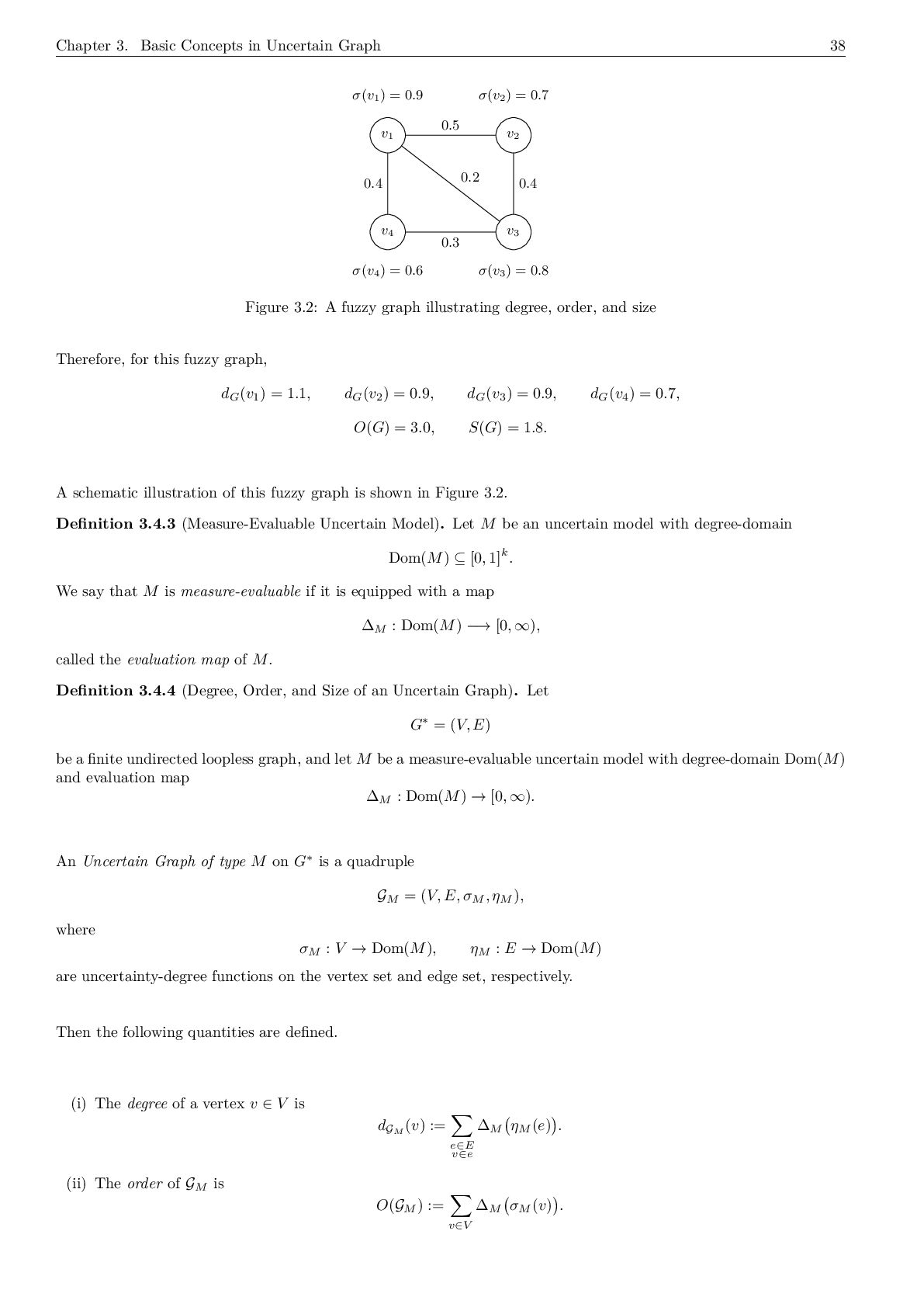
310. 309 Bibliography [282] Juhi Chaudhary, Sounaka Mishra, and Bhawani Sankar Panda. Minimum maximal acyclic matching in proper interval graphs. Discrete Applied Mathematics, 2025. [283] A. Sudhakaraiah, Telu Visalakshi, T. Venkateswarlu, and K. Narayana. Some properties on degrees of dominating sets for circular-arc graph. International Journal of Applied Engineering Research, 2021. [284] Hirotoshi Honma, Yoko Nakajima, and Atsushi Sasaki. An algorithm for the feedback vertex set problem on a normal helly circular- arc graph. Journal of Computational Chemistry, 04:23–31, 2016. [285] Ali Vardasbi, Fatemeh Sarvi, and M. de Rijke. Probabilistic permutation graph search: Black-box optimization for fairness in ranking. Proceedings of the 45th International ACM SIGIR Conference on Research and Development in Information Retrieval, 2022. [286] Sreenanda Raut and Madhumangal Pal. Generation of maximal fuzzy cliques of fuzzy permutation graph and applications. Artificial Intelligence Review, 53:1585 – 1614, 2019. [287] Shaoli Nandi, Sukumar Mondal, Sovan Samanta, Sambhu Charan Barman, Leo Mrsić, and Antonios Kalampakas. Center of trapezoid graph: Application in selecting center location to set up a private hospital. Mathematics, 2025. [288] Min-Sheng Lin and Yung-Jui Chen. Counting the number of vertex covers in a trapezoid graph. Inf. Process. Lett., 109:1187–1192, 2009. [289] Debojyoti Bhattacharya and Subhabrata Paul. Liar’s vertex-edge domination in unit disk graph. ArXiv, abs/2509.11775, 2025. [290] Chiara Vercellino, Paolo Viviani, Giacomo Vitali, Alberto Scionti, Andrea Scarabosio, Olivier Terzo, Edoardo Giusto, and Bartolomeo Montrucchio. Neural-powered unit disk graph embedding: qubits connectivity for some qubo problems. 2022 IEEE International Conference on Quantum Computing and Engineering (QCE), pages 186–196, 2022. [291] Michael A Henning, Anders Yeo, Michael A Henning, and Anders Yeo. Linear intersection hypergraphs. Transversals in Linear Uniform Hypergraphs, pages 5–9, 2020. [292] Balázs Keszegh. Coloring intersection hypergraphs of pseudo-disks. Discrete & Computational Geometry, 64:942 – 964, 2017. [293] Maria Chudnovsky, David Eppstein, and David Fischer. String graph obstacles of high girth and of bounded degree. In International Symposium Graph Drawing and Network Visualization, 2025. [294] J. Mark Keil, Debajyoti Mondal, Ehsan Moradi, and Yakov Nekrich. Finding a maximum clique in a grounded 1-bend string graph. J. Graph Algorithms Appl., 26:553–575, 2021. [295] A Nagoor Gani and D Rajalaxmi Subahashini. Properties of fuzzy labeling graph. Applied mathematical sciences, 6(70):3461–3466, 2012. [296] Hossein Rashmanlou and RA Borzooei. New concepts of fuzzy labeling graphs. International Journal of Applied and Computational Mathematics, 3:173–184, 2017. [297] Muhammad Akram and Arooj Adeel. m-polar fuzzy labeling graphs with application. Mathematics in Computer Science, 10(3):387–402, 2016. [298] I Paulraj Jayasimman and Vignesh S Devi Murugesan. Results on intuitionistic fuzzy labeling graphs. Journal of Survey in Fisheries Sciences, 10(4S):1866–1873, 2023. [299] P. K. Hemalatha Et al. A modified fuzzy labeling graph using geometric mean and harmonic mean and its application. Advances in Nonlinear Variational Inequalities, 2023. [300] S. Yahya Mohamad and S.Suganthi. Matching in fuzzy labeling graph. International Journal of Fuzzy Mathematical Archive, 2017. [301] S. Yahya Mohamad and S.Sugan thi. Energy of complete fuzzy labeling graph through fuzzy complete matching. International Journal of Mathematics Trends and Technology, 2018. [302] Sankar Sahoo and Madhumangal Pal. Intuitionistic fuzzy labeling graphs. TWMS Journal of Applied and Engineering Mathematics, 8(2):466–476, 2018. [303] M Devi, K Ameenal Bibi, Hossein Rashmanlou, and Yahya Talebi. New concepts in intuitionistic fuzzy labelling graphs. International Journal of Advanced Intelligence Paradigms, 21(3-4):267–286, 2022. [304] Ajay Devaraj and P Chellamani. Picture fuzzy labelling graphs with an application. Annals of Optimization Theory and Practice, 3(3):117–134, 2020. [305] N. Sujatha. A noval approach on picture fuzzy graceful labeling in fluid flows. Tuijin Jishu/Journal of Propulsion Technology, 2023. [306] P. Chellamani and D. Ajay. Spherical fuzzy labelling graphs. Journal of Physics: Conference Series, 1964, 2021. [307] S Sudha, M Lathamaheswari, S Broumi, and F Smarandache. Neutrosophic fuzzy magic labeling graph with its application in academic performance of the students. Neutrosophic Sets and Systems, 60(1):8, 2023. [308] A Rajkumar et al. Neutrosophic cordial labeling on helm and closed helm graph. International Journal of Neutrosophic Science (IJNS), 25(4), 2025. [309] M Ragavi and T Kannan. A study on neutrosophic cordial labeling graphs with algorithm. Statistics, Optimization & Information Computing, 2025. [310] Takaaki Fujita and Florentin Smarandache. Uncertain automata and uncertain graph grammar. Neutrosophic Sets and Systems, 74:128–191, 2024. [311] Mohamed R. Zeen El Deen. Edge even graceful labeling of some graphs. Journal of the Egyptian Mathematical Society, 27:1–15, 2019. [312] V. Rajeswari and K. Thiagarajan. Study on binary equivalent decimal edge graceful labeling. Indian journal of science and technology, 9, 2016. [313] Sarbari Mitra and Soumya Bhoumik. Graceful labeling of triangular extension of complete bipartite graph. Electron. J. Graph Theory Appl., 7:11–30, 2019. [314] Fery Firmansah, Tasari Tasari, and Muhammad Ridlo Yuwono. Odd harmonious labeling of the zinnia flower graphs. JURNAL ILMIAH SAINS, 2023.
311. Bibliography 310 [315] Ahmad Lasim, Ikhsanul Halikin, and Kristiana Wijaya. The harmonious, odd harmonious, and even harmonious labeling. BAREKENG: Jurnal Ilmu Matematika dan Terapan, 2022. [316] Anjewierden A and Aaron Rajkumar. Neutrosophic cordial labeling on helm and closed helm graph. International Journal of Neutrosophic Science, 2025. [317] Michał Tuczyński, Przemysław Wenus, and Krzysztof Węsek. On cordial labeling of hypertrees. Discrete Mathematics & Theoretical Computer Science, 21(Graph Theory), 2019. [318] K Ameenal Bibi and M Devi. Bi-magic labeling of interval valued fuzzy graph. Advances in Fuzzy Mathematics, 12(3):645–656, 2017. [319] Yu-Chang Liang, Tsai-Lien Wong, and Xuding Zhu. Anti-magic labeling of trees. Discrete mathematics, 331:9–14, 2014. [320] Toufiq Parag and A. Elgammal. Supervised hypergraph labeling. CVPR 2011, pages 2289–2296, 2011. [321] Excelsa Suli Wildhatul Jannah, Ika Hesti Agustin, Swaminathan Venkatraman, Indah Lutfiyatul Mursyidah, Ridho Alfarisi, Rafi- antika Megahnia Prihandini, et al. On (a, d)-hyperedge antimagic labeling of certain classes of hypergraphs: A new notion. In 2nd International Conference on Neural Networks and Machine Learning 2023 (ICNNML 2023), pages 173–183. Atlantis Press, 2024. [322] S Suganya and VJ Sudhakar. A study on sd prime cordial labeling of some graphs. Malaya Journal Of Mathematik, 1:625–629, 2021. [323] S Suganya and VJ Sudhakar. Sum divisor cordial labeling of various graphs. In American Institute of Physics Conference Series, 2023. [324] Tao-Ming Wang and Cheng-Chih Hsiao. On anti-magic labeling for graph products. Discrete Mathematics, 308(16):3624–3633, 2008. [325] M Devi et al. Fuzzy anti-magic labeling on some graphs. Kongunadu Research Journal, 5(1):8–14, 2018. [326] Vijayalaxmi S. Shigehalli. Radio labeling of mycielskian graph of certain graphs. International Journal of Applied Mathematics, 2025. [327] Jiaojiao Hong and Feng Li. Optimal radio labeling for strong product graph of star graph and path. 2023 IEEE 6th International Conference on Electronics and Communication Engineering (ICECE), pages 69–74, 2023. [328] Gurusamy Rengasamy Vijayakumar. A note on set graceful labeling of graphs. arXiv: Combinatorics, 2011. [329] C Karthikeyan and M Sivasubramanian. Fuzzy lucky labeling and proper fuzzy lucky labeling of special graphs. International Journal of Latest Technology in Engineering Management & Applied Science, 2025. [330] J. Ashwini, S. Selvam, and R. B. Gnanajothi. Some new results on lucky labeling. Baghdad Science Journal, 2023. [331] S Bala, S Saraswathy, and K Thirusangu. Lucky labeling for extended triplicate graph of star. Journal of Computational Mathematica, 2023. [332] J. Uma Maheswari, K. Dillibabu, and A. Anbarasan. Fuzzy detour µ-distance on direct sum of two complete fuzzy graphs. AIP Conference Proceedings, 2026. [333] Tony Yulianto, Nor Hayati, Ika Hesti Agustin, Rica Amalia, Faisol, Kuzairi, and Budi Irwansyah. Properties of cartesian multipli- cation operations in complete fuzzy graphs, effective fuzzy graphs and complement fuzzy graphs. Journal of Physics: Conference Series, 1538, 2020. [334] Talal Al-Hawary. Complete fuzzy graphs. International Journal of Mathematical Combinatorics, 4:26, 2011. [335] Kung-Jui Pai, Shyue-Ming Tang, Jou-Ming Chang, and Jinn-Shyong Yang. Completely independent spanning trees on complete graphs, complete bipartite graphs and complete tripartite graphs. In Advances in Intelligent Systems and Applications-Volume 1: Proceedings of the International Computer Symposium ICS 2012 Held at Hualien, Taiwan, December 12–14, 2012, pages 107–113. Springer, 2013. [336] Zsolt Baranyai. The edge-coloring of complete hypergraphs i. Journal of Combinatorial Theory, Series B, 26(3):276–294, 1979. [337] Dhruv Mubayi and Yi Zhao. Forbidding complete hypergraphs as traces. Graphs and Combinatorics, 23(6):667–679, 2007. [338] Jean-Claude Bermond and Vance Faber. Decomposition of the complete directed graph into k-circuits. J. Comb. Theory B, 21:146–155, 1976. [339] Nicola Apollonio. Functions that are uniquely maximized by sparse quasi-star graphs, and uniquely minimized by quasi-complete graphs. Discret. Appl. Math., 366:226–237, 2024. [340] Vladlen I. Epishin. Studying fault tolerance of bipartite homogeneous minimal quasi-complete graphs using cisco packet tracer. 2021 IEEE Conference of Russian Young Researchers in Electrical and Electronic Engineering (ElConRus), pages 318–320, 2021. [341] David F. Anderson and Shashikant Mulay. On the diameter and girth of a zero-divisor graph. Journal of Pure and Applied Algebra, 210:543–550, 2007. [342] Nilesh Khandekar and Vinayak Joshi. Zero-divisor graphs and total coloring conjecture. Soft Computing, 24:18273 – 18285, 2020. [343] Christy P. Antony and Shiny Jose. Fault-tolerant analysis in smart agriculture using intuitionistic fuzzy zero-divisor graph. New Mathematics and Natural Computation, 2025. [344] A. Kuppan and J. Ravi Sankar. Decomposition of fuzzy zero divisor graph. Journal of Physics: Conference Series, 1770, 2021. [345] Nasir Ali, Hafiz Muhammad Ahmed Siddiqui, Muhammad Imran Qureshi, Manal Elzain Mohamed Abdalla, N. S. Abd EL-Gawaad, and Fikadu Tesgera Tolasa. On study of multiset dimension in fuzzy zero divisor graphs associated with commutative rings. International Journal of Computational Intelligence Systems, 17, 2024. [346] R.Rajeswari, N.Meenakumari, and Shobha Shree. On fuzzy ideal based fuzzy zero divisor graphs on γ-near ring. Journal of emerging technologies and innovative research, 2019. [347] Elif Eryaşar and Esra Öztürk Sözen. Fuzzy f-index of fuzzy zero divisor graphs with matlab based algebraic applications. Filomat, 2025. [348] Nasir Ali, Hafiz Muhammad Afzal Siddiqui, Muhammad Imran Qureshi, Manal Elzain Mohamed Abdalla, NS Abd EL-Gawaad, and Fikadu Tesgera Tolasa. On study of multiset dimension in fuzzy zero divisor graphs associated with commutative rings. International Journal of Computational Intelligence Systems, 17(1):298, 2024.
312. 311 Bibliography [349] M Hamidi. Zero divisor graphs based on general hyperrings . Journal of Algebraic Hyperstructures and Logical Algebras, 4(2):131–149, 2023. [350] Said Broumi et al. Decomposition of neutrosophic zero-divisor graph. Neutrosophic Sets and Systems, 83(1):9, 2025. [351] Takaaki Fujita and Florentin Smarandache. A reconsideration of advanced concepts in neutrosophic graphs: Smart, zero divisor, layered, weak, semi, and chemical graphs. Advancing Uncertain Combinatorics through Graphization, Hyperization, and Uncer- tainization: Fuzzy, Neutrosophic, Soft, Rough, and Beyond, page 308, 2025. [352] K. Gunasekar and P. Muralikrishna. Graph decomposition techniques in neutrosophic zero divisor models of commutative ring. Neutrosophic Sets and Systems, 97:77–92, 2026. [353] Shane P. Redmond. An ideal-based zero-divisor graph of a commutative ring. Communications in Algebra, 31:4425 – 4443, 2003. [354] Husam Q. Mohammad, Sahbaa A Younus, and Wafa Y. Yahya. Ring classification of ideal-based zero divisor graph with vertices 9. Al-Kitab Journal for Pure Sciences, 2025. [355] Balamoorthy S., Kavaskar T., and Vidhya K. Wiener index of an ideal-based zero-divisor graph of commutative ring with unity. AKCE Int. J. Graphs Comb., 21:111–119, 2023. [356] Mohd Arif Raza and Husain S. Alhazmi. On some embedding of the strong annihilating-ideal graph of commutative rings. Filomat, 2025. [357] M. Mehrara, Mohammad Javad Nikmehr, and Reza Nikandish. Metric and strong metric dimension of essential annihilating-ideal graph of commutative rings. Discrete Mathematics, Algorithms and Applications, 2025. [358] Subramanian Visweswaran. Some remarks on the dominating sets of the annihilating-ideal graph of a commutative ring. Discussiones Mathematicae - General Algebra and Applications, 2024. [359] A. S. Monastyreva. Some properties of compressed zero-divisor graph. Mathematics and Theoretical Computer Science, 2025. [360] M. Khazaee, Mohammad Maghasedi, and Faezeh Heydari. Strong resolving graph and strong metric dimension of a compressed zero divisor graph. Journal of Algebra and Its Applications, 2025. [361] Pinkaew Siriwong and Ratinan Boonklurb. k-zero-divisor and ideal-based k-zero-divisor hypergraphs of some commutative rings. Symmetry, 13:1980, 2021. [362] Krishnan Selvakumar and V. Ramanathan. Classification of nonlocal rings with genus one 3-zero-divisor hypergraphs. Communica- tions in Algebra, 45:275 – 284, 2017. [363] Madhumangal Pal, Sovan Samanta, and Ganesh Ghorai. Fuzzy tolerance graphs. In Modern Trends in Fuzzy Graph Theory, pages 153–173. Springer, 2020. [364] Tanmoy Mahapatra and Madhumangal Pal. An investigation on m-polar fuzzy tolerance graph and its application. Neural Computing and Applications, 34:3007 – 3017, 2021. [365] Sankar Sahoo and Madhumangal Pal. Intuitionistic fuzzy tolerance graphs with application. Journal of Applied Mathematics and Computing, 55:495–511, 2017. [366] Sankar Das, Soumitra Poulik, and Ganesh Ghorai. Picture fuzzy tolerance competition graphs with its application. Journal of Ambient Intelligence and Humanized Computing, 15:547 – 559, 2023. [367] Sankar Das, Ganesh Ghorai, and Madhumangal Pal. Picture fuzzy tolerance graphs with application. Complex & Intelligent Systems, 8:541 – 554, 2021. [368] Juanjuan Lu, Linli Zhu, and Wei Gao. Cyclic connectivity index of bipolar fuzzy incidence graph. Open Chemistry, 20(1):331–341, 2022. [369] Shu Gong and Gang Hua. Topological indices of bipolar fuzzy incidence graph. Open Chemistry, 19(1):894–903, 2021. [370] S Afsharmanesh and Rajab Ali Borzooei. Domination in fuzzy incidence graphs based on valid edges. Journal of Applied Mathematics and Computing, 68(1):101–124, 2022. [371] Seyed Hossein Sadati, Hossein Rashmanlou, and Ali Asghar Talebi. Domination in intuitionistic fuzzy incidence graph. In 2021 52nd Annual Iranian Mathematics Conference (AIMC), pages 88–94. IEEE, 2021. [372] Irfan Nazeer, Tabasam Rashid, and Abazar Keikha. An application of product of intuitionistic fuzzy incidence graphs in textile industry. Complex., 2021:5541125:1–5541125:16, 2021. [373] Yongsheng Rao, Saeed Kosari, and Mehdi Gheisari. New results in vague incidence graphs with application. Journal of Function Spaces, 2022. [374] Barti Aadal Praveen and Deepa Ganesan. Edge domination and incidence domination in vague incidence graphs and its application. Symmetry, 14:1638, 2022. [375] John N. Mordeson, Sunil C. Mathew, and Rajab Ali Borzooei. Vulnerability and government response to human trafficking: Vague fuzzy incidence graphs. New Math. Nat. Comput., 14:203–219, 2018. [376] Irfan Nazeer and Tabasam Rashid. Picture fuzzy incidence graphs with application. Punjab University Journal of Mathematics, 2021. [377] Muhammad Akram, Sidra Sayed, and Florentin Smarandache. Neutrosophic incidence graphs with application. Axioms, 7:47, 2018. [378] Siti Nurul Fitriah Mohamad, Roslan Hasni, and Florentin Smarandache. Novel concepts on domination in neutrosophic incidence graphs with some applications. J. Adv. Comput. Intell. Intell. Informatics, 27:837–847, 2023. [379] Muhammad Akram, Nabeela Ishfaq, Florentin Smarandache, and Said Broumi. Application of bipolar neutrosophic sets to incidence graphs. Neutrosophic Sets and Systems, 27:17, 2019. [380] Xavier Eric Ouvrard. Hyper-bag-graphs and their applications: Modeling, Analyzing and Visualizing Complex Networks of Co- occurrences. PhD thesis, Geneva U. [381] Michelle Kendall and Keith M Martin. Graph-theoretic design and analysis of key predistribution schemes. Designs, Codes and Cryptography, 81(1):11–34, 2016. [382] Takaaki Fujita and Florentin Smarandache. HyperGraph and SuperHyperGraph Theory with Applications (VI): Graph Structure (Path, Tree, Cycle, Planarity, Bipartite, and More). Infinite Study, 2026.
313. Bibliography 312 [383] Lucas J Rusnak. Oriented hypergraphs i: Introduction and balance. arXiv preprint arXiv:1210.0943, 2012. [384] Daniël Paulusma, Friedrich Slivovsky, and Stefan Szeider. Model counting for cnf formulas of bounded modular treewidth. Algorith- mica, 76(1):168–194, 2016. [385] Eduard Eiben, Robert Ganian, Dusan Knop, Sebastian Ordyniak, et al. Unary integer linear programming with structural restrictions. In IJCAI, pages 1284–1290, 2018. [386] A Kaveh and HA Rahimi Bondarabady. A hybrid graph-genetic method for domain decomposition. Finite elements in analysis and design, 39(13):1237–1247, 2003. [387] A Kaveh and HA Rahimi Bondarabady. Spectral trisection of finite element models. International Journal of Numerical Methods for Heat & Fluid Flow, 11(4):358–370, 2001. [388] Persi Diaconis, Susan Holmes, and Svante Janson. Threshold graph limits and random threshold graphs. Internet Mathematics, 5(3):267–320, 2008. [389] Nadimpalli VR Mahadev and Uri N Peled. Threshold graphs and related topics, volume 56. Elsevier, 1995. [390] Muhammad Akram, Uzma Ahmad, Rukhsar, and Faruk Karaaslan. Complex pythagorean fuzzy threshold graphs with application in petroleum replenishment. journal of applied mathematics and computing, 68(3):2125–2150, 2022. [391] Lanzhen Yang and Hua Mao. Intuitionistic fuzzy threshold graphs. Journal of Intelligent & Fuzzy Systems, 36(6):6641–6651, 2019. [392] Sankar Das, Ganesh Ghorai, and Qin Xin. Picture fuzzy threshold graphs with application in medicine replenishment. Entropy, 24(5):658, 2022. [393] Sovan Samanta and Madhumangal Pal. Fuzzy threshold graphs. CIIT International Journal of Fuzzy Systems, 3(12):360–364, 2011. [394] Lanzhen Yang and Hua Mao. Intuitionistic fuzzy threshold graphs. J. Intell. Fuzzy Syst., 36:6641–6651, 2019. [395] Saira Hameed, Muhammad Akram, Noreen Mustafa, and Faruk Karaaslan. Extension of threshold graphs under complex intuitionistic fuzzy environment. J. Multiple Valued Log. Soft Comput., 37:295–315, 2021. [396] Myithili.K.K. Intuitionistic fuzzy threshold hypergraphs and their role in chasing fugitives with multi-bots. Communications on Applied Nonlinear Analysis, 2024. [397] Takaaki Fujita. Note for neutrosophic incidence and threshold graph. SciNexuses, 2024. [398] Robert E Jamison and Alan P Sprague. Multithreshold graphs. Journal of Graph Theory, 94(4):518–530, 2020. [399] Gregory J Puleo. Some results on multithreshold graphs. Graphs and Combinatorics, 36(3):913–919, 2020. [400] Jan Reiterman, Vojtěch Rödl, Edita Šiňajová, and Miroslav Tuma. Threshold hypergraphs. Discrete Mathematics, 54(2):193–200, 1985. [401] Anirban Banerjee, Rajiv Mishra, and Samiron Parui. On the spectra of threshold hypergraphs. arXiv preprint arXiv:2207.02528, 2022. [402] Nina Chiarelli and Martin Milanič. Total domishold graphs: a generalization of threshold graphs, with connections to threshold hypergraphs. Discrete Applied Mathematics, 179:1–12, 2014. [403] R. Abirami and N. Sarala. Rainbow coloring of magic fuzzy random graphs. Communications in Mathematics and Applications, 2024. [404] Sarala N and Abirami Ravichandran. Beta and gamma products of fuzzy random graphs with hesitancy. Malaysian Journal of Fundamental and Applied Sciences, 2024. [405] N. Sarala and R. Abirami. On topological indices of fuzzy random graph. Indian Journal Of Science And Technology, 2024. [406] Tatiana A. Makarenya, Ali Sajae Mannaa, Alexey I. Kalinichenko, and Svetlana V. Petrenko. Fuzzy cognitive maps: approaches to construction and analysis. International Journal on Smart Sensing and Intelligent Systems, 19, 2026. [407] Michal Puheim, Ján Vascák, and Ladislav Madarász. Three-term relation neuro-fuzzy cognitive maps. 2014 IEEE 15th International Symposium on Computational Intelligence and Informatics (CINTI), pages 477–482, 2014. [408] Alexander Bozhenyuk, Stanislav Belyakov, Margarita Knyazeva, and Vitalii Bozheniuk. Temporal reachability in fuzzy graphs for geographic information systems. In International Conference on Intelligent Information Technologies for Industry, pages 507–516. Springer, 2019. [409] Sankar Chakaravarthy, Kalaivani Chandran, Perumal Chellamani, and Gangatharan Venkat Narayanan. Analyzing network stability via symmetric structures and domination integrity in signed fuzzy graphs. Symmetry, 17:766, 2025. [410] Sankar Chakaravarthy, Mariappan Saravanan, Ramalingam Sujatha, and Gangatharan Venkat Narayanan. Signed fuzzy graphs domination in environmental monitoring wireless sensor networks. European Journal of Pure and Applied Mathematics, 2025. [411] Chakaravarthy Sankar, C. T. Kalaivani, Mariappan Saravanan, and Ramalingam Sujatha. An algorithmic approach to signed fuzzy graph integrity: Complexity, graph operations, and metro rail network applications. Ain Shams Engineering Journal, 2025. [412] Xin Ma and Dazi Li. A hybrid fault diagnosis method based on fuzzy signed directed graph and neighborhood rough set. 2017 6th Data Driven Control and Learning Systems (DDCLS), pages 253–258, 2017. [413] L Jagadeeswari and VJ Sudhakar. Bipolar interval valued signed neutrosophic graphs. Malaya Journal of Matematik, 9(1):1086–1094, 2021. [414] VJ Sudhakar, D Vinoth, G Sathishkumr, et al. Self-centered interval valued signed neutrosophic graphs. International journal of Mathematical Archive, 9(9):44–50, 2016. [415] VJ Sudhakar, Ali A Mohamed, and D Vinoth. Interval valued signed neutrosophic graph. Infinite Study, 2016. [416] Utti Marina Rifanti and Bongga Arifwidodo. Tourism transportation’s optimum route in banyumas using the weighted fuzzy graph. THE 2ND INTERNATIONAL CONFERENCE ON SCIENCE, MATHEMATICS, ENVIRONMENT, AND EDUCATION, 2019. [417] Alexander M. Banaru, Daria A. Banaru, and Sergey M. Aksenov. Groupoid of intermolecular contacts and its fuzzy cayley graph. Moscow University Chemistry Bulletin, 78:103–113, 2023. [418] JISHA MARY JOHN and A. Riyas. Cayley fuzzy graph representations of groups with emphasis on subgroup and left coset hierarchies. Proyecciones (Antofagasta), 2025.
314. 313 Bibliography [419] Mary John Jisha, A. Riyas, and K. N. Geetha. Cayley fuzzy graphs on groups. Proyecciones (Antofagasta), 2024. [420] M. H. Shahzamanian and Bijan Davvaz. Roughness in fuzzy cayley graphs. BULLETIN OF THE KARAGANDA UNIVERSITY- MATHEMATICS, 2023. [421] RA Borzooei and Hossein Rashmanlou. Cayley interval-valued fuzzy graphs. UPB Scientific Bulletin, Series A: Applied Mathematics and Physics, 78(3):83–94, 2016. [422] Ali Asghar Talebi. Cayley fuzzy graphs on the fuzzy groups. Computational and Applied Mathematics, 37:4611–4632, 2018. [423] Waheed Ahmad Khan, Khurram Faiz, and Abdelghani Taouti. Cayley picture fuzzy graphs and interconnected networks. Intell. Autom. Soft Comput., 35:3317–3330, 2023. [424] Amir Sabir Majeed. Cayley neutrosophic graphs on the neutrosophic groups. JOURNAL OF UNIVERSITY OF BABYLON for Pure and Applied Sciences, 2024. [425] Charles M Fiduccia, Rodney W Forcade, and Jennifer S Zito input epsf. Geometry and diameter bounds of directed cayley graphs of abelian groups. SIAM Journal on Discrete Mathematics, 11(1):157–167, 1998. [426] Charles Celerier, David Joyner, Caroline Melles, David Phillips, and Steven Walsh. Explorations of edge-weighted cayley graphs and p-ary bent functions. arXiv preprint arXiv:1406.1087, 2014. [427] Deepa Sinha, Ayushi Dhama, and BD Acharya. Unitary addition cayley signed graphs. European Journal of Pure and Applied Mathematics, 6(2):189–210, 2013. [428] Majid Arezoomand, Afshin Behmaram, Mohsen Ghasemi, and Parivash Raeighasht. Isomorphisms of bi-cayley graphs on dihedral groups. Discrete Mathematics, Algorithms and Applications, 12(04):2050051, 2020. [429] Changqun Wang. Bi-cayley graphs of a. Ars Combinatoria, 80:177–187, 2006. [430] Abolfazl Nikkhah and Bijan Davvaz. Cayley hypergraph over polygroups. Transactions on Combinatorics, 14(1), 2025. [431] Adel Hlaoui and Shengrui Wang. A new median graph algorithm. In Workshop on Graph Based Representations in Pattern Recognition, 2003. [432] Salim Jouili, Salvatore Tabbone, and Vinciane Lacroix. Median graph shift: A new clustering algorithm for graph domain. 2010 20th International Conference on Pattern Recognition, pages 950–953, 2010. [433] Miquel A. Ferrer, Ernest Valveny, Francesc Serratosa, Kaspar Riesen, and Horst Bunke. Generalized median graph computation by means of graph embedding in vector spaces. Pattern Recognit., 43:1642–1655, 2010. [434] Anandhu Mohan, M. V. Dhanyamol, and Sunil Mathew. The structural properties of fuzzy median graphs. Journal of Applied Mathematics and Computing, 2024. [435] Anandhu Mohan, M. V. Dhanyamol, and Vidya Sagar Thalapala. Fuzzy median graph algorithm for facility location problem. 2nd INTERNATIONAL CONFERENCE ON COMPUTATIONAL SCIENCES-MODELLING, COMPUTING AND SOFT COMPUT- ING (CSMCS 2022), 2023. [436] Anandhu Mohan, Vidya Sagar Thalapala, Koppala Guravaiah, and M. V. Dhanyamol. Fmgnr: fuzzy median graph for network routing applications. Wireless Networks, 29:821–832, 2022. [437] Emiel Claasen and Mehregan Doroudiani. From modular graph forms to iterated integrals. Journal of High Energy Physics, 2025. [438] Ryan Lorig-Roach, Melissa Meredith, Jean Monlong, Miten Jain, Hugh E. Olsen, Brandy McNulty, David Porubsky, Tessa Montague, Julian K. Lucas, Chris Condon, Jordan M. Eizenga, Sissel Juul, Sean Mckenzie, Sara E. Simmonds, Jimin Park, Mobin Asri, Sergey Koren, Evan E. Eichler, Richard Axel, Bruce Martin, Paolo Carnevali, Karen H. Miga, and Benedict Paten. Phased nanopore assembly with shasta and modular graph phasing with gfase. bioRxiv, 2023. [439] Sven Herrmann and Vincent Moulton. Computing the blocks of a quasi-median graph. ArXiv, abs/1206.6135, 2012. [440] Motiejus Valiunas. Acylindrical hyperbolicity of groups acting on quasi-median graphs and equations in graph products. Groups, Geometry, and Dynamics, 2018. [441] Carolyn Abbott, Anthony Genevois, and Eduardo Martinez-Pedroza. Homotopy types of complexes of hyperplanes in quasi-median graphs and applications to right-angled artin groups. arXiv preprint arXiv:2503.08411, 2025. [442] Hans-Jürgen Bandelt and Henry Martyn Mulder. Pseudo-median graphs: decomposition via amalgamation and cartesian multipli- cation. Discret. Math., 94:161–180, 1991. [443] Hans-Jürgen Bandelt and Henry Martyn Mulder. Regular pseudo-median graphs. J. Graph Theory, 12:533–549, 1988. [444] Hans-Jürgen Bandelt and Henry Martyn Mulder. Pseudo-median graphs are join spaces. Discret. Math., 109:13–26, 1992. [445] Kousik Das, Sovan Samanta, and Kajal De. Fuzzy chordal graphs and its properties. International Journal of Applied and Compu- tational Mathematics, 7, 2021. [446] A. Shajitha and Sameena Kalathodi. A study on fuzzy chordal graphs. Malaya Journal of Matematik, 2019. [447] A. Shajitha and Sameena Kalathodi. On the center of fuzzy strong chordal graphs. New Math. Nat. Comput., 21:409–414, 2024. [448] Keneni Abera Tola, VN Srinivasa Rao Repalle, and Mamo Abebe Ashebo. Interval-valued bipolar fuzzy line graphs. BMC Research Notes, 16(1):118, 2023. [449] Muhammad Akram and Arooj Adeel. m-polar fuzzy graphs and m-polar fuzzy line graphs. Journal of Discrete Mathematical Sciences and Cryptography, 20:1597 – 1617, 2017. [450] VN Srinivasa Rao Repalle, Keneni Abera Tola, and Mamo Abebe Ashebo. Interval valued intuitionistic fuzzy line graphs. BMC Research Notes, 15(1):250, 2022. [451] Muhammad Akram and R Parvathi. Properties of intuitionistic fuzzy line graphs. Notes on intuitionistic fuzzy sets, 18(3):52–60, 2012. [452] Venkata Naga Srinivasa Rao Repalle, Keneni Abera Tola, and Maamo Abebe Ashebo. Extended intuitionistic fuzzy line graphs: Theory and properties. In Coding Theory Essentials. IntechOpen, 2023. [453] Annamalai Meenakshi, J Shivangi Mishra, Leo Mršić, Antonios Kalampakas, Sovan Samanta, and Tofigh Allahviranloo. Maximal product-based intuitionistic fuzzy line graphs for healthcare predictive analysis. Ain Shams Engineering Journal, page 103939, 2026.
315. Bibliography 314 [454] Muhammad Akram, Musavarah Sarwar, and Wieslaw A Dudek. Graphs for the analysis of bipolar fuzzy information, volume 401. Springer, 2021. [455] Muhammad Akram, Musavarah Sarwar, and Wieslaw A Dudek. Special types of bipolar fuzzy graphs. In Graphs for the Analysis of Bipolar Fuzzy Information, pages 127–159. Springer, 2020. [456] Muhammad Akram and Wieslaw A Dudek. Regular bipolar fuzzy graphs. Neural computing and applications, 21(Suppl 1):197–205, 2012. [457] Zhihua Chen, Waheed Ahmad Khan, and Aysha Khan. Concepts of picture fuzzy line graphs and their applications in data analysis. Symmetry, 15(5):1018, 2023. [458] Muhammad Akram and Amna Habib. q-rung picture fuzzy graphs: A creative view on regularity with applications. Journal of Applied Mathematics and Computing, 61(1):235–280, 2019. [459] Sumera Naz and Muhammad Aslam Malik. Single-valued neutrosophic line graphs. TWMS Journal of Applied and Engineering Mathematics, 8(2):483–494, 2018. [460] Keneni Abera Tola, VN Srinivasa Rao Repalle, and Mamo Abebe Ashebo. Theory and application of interval-valued neutrosophic line graphs. Journal of Mathematics, 2024(1):5692756, 2024. [461] Toru Hasunuma. Queue layouts of iterated line directed graphs. Discrete applied mathematics, 155(9):1141–1154, 2007. [462] Yehong Shao. Connectivity of iterated line graphs. Discrete applied mathematics, 158(18):2081–2087, 2010. [463] Liming Xiong and Zhanhong Liu. Hamiltonian iterated line graphs. Discrete mathematics, 256(1-2):407–422, 2002. [464] Toru Hasunuma and Mayu Otani. On the (h, k)-domination numbers of iterated line digraphs. Discrete Applied Mathematics, 160(12):1859–1863, 2012. [465] Mahipal Jadeja, Rahul Muthu, and Ravi Goyal. A new characterisation of total graphs. Palestine Journal of Mathematics, 13(4), 2024. [466] Lyra Yulianti, Admi Nazra, et al. On the rainbow connection numbers of line, middle, and total graphs of wheels. Electronic Journal of Graph Theory & Applications, 13(1), 2025. [467] Eber Lenes, Exequiel Mallea-Zepeda, María Robbiano, and Jonnathan Rodríguez. On the diameter and incidence energy of iterated total graphs. Symmetry, 10(7):252, 2018. [468] Gui-Xian Tian. The asymptotic behavior of (degree-) kirchhoff indices of iterated total graphs of regular graphs. Discrete Applied Mathematics, 233:224–230, 2017. [469] RI Tyshkevich and Vadim E Zverovich. Line hypergraphs. Discrete Mathematics, 161(1-3):265–283, 1996. [470] Regina I Tyshkevich and Vadim E Zverovich. Line hypergraphs: A survey. Acta Applicandae Mathematica, 52(1-3):209–222, 1998. [471] Takaaki Fujita. Note for line and total superhypergraphs: Connecting vertices, edges, edges of edges, edges of edges of edges in hierarchical systems. Journal of Mathematical Analysis and Modeling, 6(3):11–43, 2025. [472] Xia-an Bi, Zicheng Yang, Dayou Chen, Jie Wang, Zhaoxu Xing, and Luyun Xu. Fhg-gan: Fuzzy hypergraph generative adversarial network with large foundation models for alzheimer’s disease risk prediction. IEEE Transactions on Fuzzy Systems, 2025. [473] Ramin Tabatabaei Mirhosseini. Evaluation of seismic vulnerability using clustering based on fuzzy hypergraphs. In Structures, volume 73, page 108457. Elsevier, 2025. [474] Annamalai Meenakshi, Obel Mythreyi, Leo Mrsic, Antonios Kalampakas, and Sovan Samanta. A fuzzy hypergraph-based framework for secure encryption and decryption of sensitive messages. Mathematics, 13(7):1049, 2025. [475] Nandhini Chandrasekar et al. Some statistical tools on intuitionistic fuzzy threshold hypergraphs. Big Data and Computing Visions, page e226483, 2025. [476] KK Myithili and C Nandhini. Analysis of hub parameters in fuzzy hypergraphs extending to intuitionistic fuzzy threshold hyper- graphs: Applications in designing transport networks in amusement parks using hub hyperpaths. Notes on Intuitionistic Fuzzy Sets, 30(3), 2024. [477] KK Myithili and C Nandhini. Transversals and its properties of intuitionistic fuzzy threshold hypergraphs. In Fuzzy Logic Concepts in Computer Science and Mathematics, pages 59–73. Apple Academic Press, 2025. [478] Ali Hassan, Muhammad Aslam Malik, and Florentin Smarandache. Regular and totally regular interval valued neutrosophic hyper- graphs. Infinite Study, 2016. [479] Muhammad Aslam Malik, Ali Hassan, Said Broumi, Assia Bakali, Mohamed Talea, and Florentin Smarandache. Isomorphism of interval valued neutrosophic hypergraphs. Infinite Study, 2016. [480] Muhammad Aslam Malik, Ali Hassan, Said Broumi, Assia Bakali, Mohamed Talea, and Florentin Smarandache. Isomorphism of bipolar single valued neutrosophic hypergraphs. Collected Papers. Volume IX: On Neutrosophic Theory and Its Applications in Algebra, page 72, 2022. [481] Florentin Smarandache. Extension of HyperGraph to n-SuperHyperGraph and to Plithogenic n-SuperHyperGraph, and Extension of HyperAlgebra to n-ary (Classical-/Neutro-/Anti-) HyperAlgebra. Infinite Study, 2020. [482] Takaaki Fujita. Metahypergraphs, metasuperhypergraphs, and iterated metagraphs: Modeling graphs of graphs, hypergraphs of hypergraphs, superhypergraphs of superhypergraphs, and beyond. Current Research in Interdisciplinary Studies, 4(5):1–23, 2025. [483] Mohammad Hamidi, Florentin Smarandache, and Elham Davneshvar. Spectrum of superhypergraphs via flows. Journal of Mathe- matics, 2022(1):9158912, 2022. [484] Yan Cao. Integrating treesoft and hypersoft paradigms into urban elderly care evaluation: A comprehensive n-superhypergraph approach. Neutrosophic Sets and Systems, 85:852–873, 2025. [485] E. J. Mogro, J. R. Molina, G. J. S. Canas, and P. H. Soria. Tree tobacco extract (Nicotiana glauca) as a plithogenic bioinsecticide alternative for controlling fruit fly (Drosophila immigrans) using n-superhypergraphs. Neutrosophic Sets and Systems, 74:57–65, 2024. [486] Takaaki Fujita and Florentin Smarandache. HyperGraph and SuperHyperGraph Theory with Applications. Neutrosophic Science International Association (NSIA) Publishing House, 2026.
316. 315 Bibliography [487] Mohammad Hamidi and Mohadeseh Taghinezhad. Application of Superhypergraphs-Based Domination Number in Real World. Infinite Study, 2023. [488] Mohammed Alqahtani. Intuitionistic fuzzy quasi-supergraph integration for social network decision making. International Journal of Analysis and Applications, 23:137–137, 2025. [489] T. Fujita, Muhammad Saqlain, and Muhammad Gulistan. Hierarchical network modeling with intuitionistic fuzzy superhypergraphs. Multicriteria Algorithms with Applications, 10(1):1–22, 2026. [490] Ehab Roshdy, Marwa Khashaba, and Mariam Emad Ahmed Ali. Neutrosophic super-hypergraph fusion for proactive cyberattack countermeasures: A soft computing framework. Neutrosophic Sets and Systems, 94:232–252, 2025. [491] Shouxian Zhu. Neutrosophic n-superhypernetwork: A new approach for evaluating short video communication effectiveness in media convergence. Neutrosophic Sets and Systems, 85:1004–1017, 2025. [492] Takaaki Fujita and Florentin Smarandache. Neutrosophic soft n-super-hypergraphs with real-world applications. Infinite Study, 2025. [493] Rajab Ali Borzooei and R. Almallah. Inverse fuzzy multigraphs and planarity with application in decision-making. Soft Computing, 26:1531 – 1539, 2021. [494] Krassimir Atanassov, Basil K Papadopoulos, and Apostolos Syropoulos. An application of the theory of intutionistic fuzzy multi- graphs. Mathware & soft computing, 11(1):45–49, 2004. [495] M Baghernejad and Rajab Ali Borzooei. Vague multigraphs: M. baghernejad, ra borzooei. Soft Computing, 23(23):12607–12619, 2019. [496] Ganesh Ghorai and Madhumangal Pal. Planarity in vague graphs with application. Acta Mathematica Academiae Paedagogicae Nyiregyhaziensis, 33(2):147–164, 2017. [497] Nahlia Rakhmawati, Agus Widodo, Noor Hidayat, and Abdul Rouf Alghofari. Optimal path with interval value of intuitionistic fuzzy number in multigraph. IAENG International Journal of Computer Science, 51(1):39–44, 2024. [498] Noura Alshehri and Muhammad Akram. Intuitionistic fuzzy planar graphs. Discrete Dynamics in Nature and Society, 2014(1):397823, 2014. [499] Muhammad Akram, Musavarah Sarwar, and Wieslaw A Dudek. Bipolar fuzzy planar graphs. In Graphs for the Analysis of Bipolar Fuzzy Information, pages 223–251. Springer, 2020. [500] Tarasankar Pramanik, Madhumangal Pal, Sukumar Mondal, and Sovan Samanta. A study on bipolar fuzzy planar graph and its application in image shrinking. Journal of Intelligent & Fuzzy Systems, 34(3):1863–1874, 2018. [501] Muhammad Akram, Sovan Samanta, and Madhumangal Pal. Application of bipolar fuzzy sets in planar graphs. International Journal of Applied and Computational Mathematics, 3(2):773–785, 2017. [502] Waheed Ahmad Khan, Khurram Faiz, and Abdelghani Taouti. Cayley picture fuzzy graphs and interconnected networks. Intelligent Automation & Soft Computing, 2022. [503] P Chellamani, D Ajay, Mohammed M Al-Shamiri, and Rashad Ismail. Pythagorean Neutrosophic Planar Graphs with an Application in Decision-Making. Infinite Study, 2023. [504] WB Vasantha Kandasamy, K Ilanthenral, and Florentin Smarandache. Subset Vertex Multigraphs and Neutrosophic Multigraphs for Social Multi Networks. Infinite Study, 2019. [505] J Abderramán Marrero, Juan Núñez Valdés, and María Trinidad Villar. Associating hub-directed multigraphs to arrowhead matrices. Mathematical Methods in the Applied Sciences, 41(6):2360–2369, 2018. [506] Takaaki Fujita. Hyperweighted and superhyperweighted multigraphs: Foundations and real-world applications. Soft Computing Fusion with Applications, 2025. [507] Benjamin R Smith. Cycle decompositions of complete multigraphs. Journal of Combinatorial Designs, 18(2):85–93, 2010. [508] Zhihe Liang and Jinping Guo. Decomposition of complete multigraphs into crown graphs. Journal of Applied Mathematics and Computing, 32(2):507–517, 2010. [509] Darryn Bryant, Daniel Horsley, Barbara Maenhaut, and Benjamin R Smith. Cycle decompositions of complete multigraphs. Journal of Combinatorial Designs, 19(1):42–69, 2011. [510] Noga Alon. A simple algorithm for edge-coloring bipartite multigraphs. Information Processing Letters, 85(6):301–302, 2003. [511] Mahyar Afshinmehr, Alireza Danaei, Mehrafarin Kazemi, Kurt Mehlhorn, and Nidhi Rathi. Efx allocations and orientations on bipartite multi-graphs: A complete picture. arXiv preprint arXiv:2410.17002, 2024. [512] Jan Bok, Jiří Fiala, Nikola Jedličková, Jan Kratochvíl, and Paweł Rzążewski. List covering of regular multigraphs. In International Workshop on Combinatorial Algorithms, pages 228–242. Springer, 2022. [513] Haim Kaplan, Moshe Lewenstein, Nira Shafrir, and Maxim Sviridenko. Approximation algorithms for asymmetric tsp by decomposing directed regular multigraphs. Journal of the ACM (JACM), 52(4):602–626, 2005. [514] M Baghernejad and Rajab Ali Borzooei. Results on soft graphs and soft multigraphs with application in controlling urban traffic flows. Soft Computing, 27(16):11155–11175, 2023. [515] Ziang Li, Jie Wu, Guojing Han, Chi Ma, and Yuenai Chen. Multi-hypergraph neural network with fusion of location information for session-based recommendation. IAENG International Journal of Applied Mathematics, 53(4), 2023. [516] Zhe Yang, Liangkui Xu, and Lei Zhao. Efbh: Collaborative filtering model based on multi-hypergraph encoder. IEEE Transactions on Consumer Electronics, 70(1):2939–2948, 2023. [517] Le An, Xiaojing Chen, Songfan Yang, and Xuelong Li. Person re-identification by multi-hypergraph fusion. IEEE transactions on neural networks and learning systems, 28(11):2763–2774, 2016. [518] Qinghua Liu, Xiaojiao Chen, and Xiaoteng Tang. Spherical fuzzy bipartite graph based qfd methodology (sfbg-qfd): Assistive products design application. Expert Syst. Appl., 239:122279, 2024. [519] Shanookha Ali. Hardness and structural properties of fuzzy edge contraction. arXiv preprint arXiv:2509.16185, 2025. [520] A Balakrishnan and K Thiruganasambandam. Neutrosophic topologized bipartite graph. Reliability: Theory & Applications, 20(4 (89)):105–113, 2025.
317. Bibliography 316 [521] Florentin Smarandache, WB Kandasamy, and K Ilanthenral. MOD Graphs. EuropaNova, Brussels, 2016. [522] WB Vasantha Kandasamy and Florentin Smarandache. Basic neutrosophic algebraic structures and their application to fuzzy and neutrosophic models, volume 4. Infinite Study, 2004. [523] Zi-Ke Zhang, Tao Zhou, and Yi-Cheng Zhang. Personalized recommendation via integrated diffusion on user–item–tag tripartite graphs. Physica A: Statistical Mechanics and its Applications, 389(1):179–186, 2010. [524] Tristan Jenkinson, John Kenneth Truss, and Daniel Seidel. Countable homogeneous multipartite graphs. Eur. J. Comb., 33:82–109, 2012. [525] Deborah C. Lockett and John Kenneth Truss. Homogeneous coloured multipartite graphs. Eur. J. Comb., 42:217–242, 2014. [526] Zoltän Füredi. Intersection representations of the complete bipartite graph. The Mathematics of Paul Erdös II, pages 86–92, 1997. [527] Hussain R Jahir and Farhana M Afya. Bounds on fuzzy dominator chromatic number of fuzzy soft bipartite graphs. Ratio Mathe- matica, 46, 2023. [528] K. Kalaiarasi and L. Mahalakshmi. Fuzzy soft tri-partite graphs and its complement. Journal of Mathematical Control Science and Applications, 7(1), 2021. [529] Kuo Chen and Cuiping Kuang. Web service discovery based on maximum weighted bipartite graphs. Computer Communications, 171:54–60, 2021. [530] Yuta Harada, Hirotaka Ono, Kunihiko Sadakane, and Masafumi Yamashita. Optimal balanced semi-matchings for weighted bipartite graphs. Information and Media Technologies, 2(4):1103–1112, 2007. [531] Chor Ping Low. An approximation algorithm for the load-balanced semi-matching problem in weighted bipartite graphs. Information Processing Letters, 100(4):154–161, 2006. [532] Muhammad Akram and Ayesha Khan. Complex pythagorean dombi fuzzy graphs for decision making. Granular Computing, 6:645 – 669, 2020. [533] Muhammad Akram, Jawaria Mohsan Dar, and Sumera Naz. Pythagorean dombi fuzzy graphs. Complex & Intelligent Systems, 6(1):29–54, 2020. [534] Ehsan Mehboob Ahmed Butt, Waqas Mahmood, Adel Fahad Alrasheedi, Jungeun Kim, and Muhammad Shoaib. Notion of complex spherical dombi fuzzy graph and its application in decision-making problems. IEEE access, 11:128429–128450, 2023. [535] S Ashraf, S Naz, and EE Kerre. Dombi fuzzy graphs. Fuzzy information and engineering, 10(1):58–79, 2018. [536] Ehsan Mehboob Ahmed Butt, Waqas Mahmood, Ferdous MO Tawfiq, Qin Xin, and Muhammad Shoaib. A study of complex dombi fuzzy graph with application in decision making problems. IEEE Access, 10:102064–102075, 2022. [537] Muhammad Akram and Ayesha Khan. Complex pythagorean dombi fuzzy graphs for decision making. Granular Computing, 6:645–669, 2021. [538] Tejinder Singh Lakhwani, Kartick Mohanta, Arindam Dey, Sankar Prasad Mondal, and Anita Pal. Some operations on dombi neutrosophic graph. Journal of Ambient Intelligence and Humanized Computing, pages 1–19, 2022. [539] Mohammad Hamidi and Florentin Smarandache. Valued-inverse dombi neutrosophic graph and application. Collected Papers, Volume XV: Neutrosophic Theories and Applications, page 199, 2025. [540] P Chellamani and D Ajay. Pythagorean neutrosophic dombi fuzzy graphs with an application to mcdm. Neutrosophic Sets and Systems, 47:411–431, 2021. [541] TK Mathew Varkey and AM Shyla. A note on bipartite and balanced fuzzy graph structures. International journal of innovative research in science, 6(7):12637–12639, 2017. [542] TALAL Al-Hawary. Maximal strong product and balanced fuzzy graphs. Journal of applied mathematics & informatics, 41(5):1145–1153, 2023. [543] K Sankar and Devarasan Ezhilmaran. Balanced bipolar intuitionistic fuzzy graphs. International Research Journal of Engineering and Technology (IRJET), 3(11):806–812, 2016. [544] N Jicy and Sunil Mathew. Connectivity analysis of cyclically balanced fuzzy graphs. Fuzzy information and Engineering, 7(2):245–255, 2015. [545] PK Kishore Kumar, S Lavanya, Sh A Safarisabet, AA Talebi, and Hossein Rashmanlou. New concepts on mild balanced vague graphs with application. International Journal of Fuzzy Mathematical Archive, 15(1):37–53, 2018. [546] Hossein Rashmanlou and Rajab Ali Borzooei. A note on vague graphs. Algebraic Structures and Their Applications, 2(1):11–22, 2015. [547] M. G. Karunambigai, Muhammad Akram, S. Sivasankar, and Kaliyaperumal Palanivel. Balanced intuitionistic fuzzy graphs. Applied mathematical sciences, 7:2501–2514, 2013. [548] Muhammad Akram, MG Karunambigai, K Palanivel, and S Sivasankar. Balanced bipolar fuzzy graphs. Journal of advanced research in pure mathematics, 6(4):58–71, 2014. [549] Biswajit Some, Parikshit Das, and Anita Pal. Balance spherical fuzzy graph and their applications. TWMS Journal of Applied and Engineering Mathematics, 2025. [550] S Sivasankar and Said Broumi. Balanced neutrosophic graphs. Neutrosophic Sets and Systems, 50:309–319, 2022. [551] Said Broumi, S Sivasankar, Assia Bakali, and Mohamed Talea. Balanced neutrosophic fermatean graphs with applications. In Analytical Decision Making and Data Envelopment Analysis: Advances and Challenges, pages 413–431. Springer, 2024. [552] Kishore Kumar PK and S Sangeetha. Mild balanced neutrosophic graphs with application. Neutrosophic Sets & Systems, 97, 2026. [553] S Sivasankar and Said Broumi. A new algorithm to determine the density of a balanced neutrosophic graph and its application to enhance education quality. In Handbook of research on the applications of neutrosophic sets theory and their extensions in education, pages 1–17. IGI Global Scientific Publishing, 2023. [554] QM Mahioub and AA Haifa. The global domination number in product fuzzy graphs. EPH, International Journal of Mathematics and statistics, pages 06–76, 2020.
318. 317 Bibliography [555] TALAL ALI AL-HAWARY and MAREF YM ALZOUBI. β-product of product fuzzy graphs. Journal of applied mathematics & informatics, 42(2):283–290, 2024. [556] T. Bharathi and S. Leo. Distance in plithogenic product fuzzy graphs. Proyecciones (Antofagasta), 2023. [557] T. Bharathi, S. Leo, and Bijan Davvaz. Domination in plithogenic product fuzzy graphs. Journal of Applied Mathematics, Statistics and Informatics, 19:5 – 22, 2023. [558] AL-Hawary Talal and Bayan Hourani. On intuitionistic product fuzzy graphs. Italian Journal of Pure and Applied Mathematics, 38:113–126, 2017. [559] T. Ali Al-Hawary. Anti product fuzzy graphs. International Journal of Apllied Mathematics, 2024. [560] Talal Al-Hawary and Bayan Horani. On product fuzzy graphs. Annals of fuzzy mathematics and Informatics, 12(2):279–294, 2016. [561] Hossein Rashmanlou, Sovan Samanta, Madhumangal Pal, and Rajab Ali Borzooei. Product of bipolar fuzzy graphs and their degree. International Journal of General Systems, 45(1):1–14, 2016. [562] Wei Ming, Areen Rasool, Umar Ishtiaq, Sundas Shahzadi, Mubariz Garayev, and Ioan-Lucian Popa. Optimizing decision-making using domination theory in product bipolar fuzzy graphs. Symmetry, 17(4):479, 2025. [563] Sankar Sahoo and Madhumangal Pal. Product of intuitionistic fuzzy graphs and degree. Journal of Intelligent & Fuzzy Systems, 32(1):1059–1067, 2017. [564] Abida Anwar and Faryal Chaudhry. On certain products of complex intuitionistic fuzzy graphs. Journal of Function Spaces, 2021(1):6515646, 2021. [565] Kartick Mohanta, Arindam Dey, and Anita Pal. A note on different types of product of neutrosophic graphs. Complex & Intelligent Systems, 7(2):857–871, 2021. [566] Zhang Guang-Ming and Cui Zhi-Ming. A novel image classification model based on contourlet transform and dynamic fuzzy graph cuts. Appl. Math, 6(1S):93S–97S, 2012. [567] Victor Kureichik and Evgeniya Gerasimenko. Method of the maximum dynamic flow finding in the fuzzy graph with gains. In International Conference on Intelligent Information Technologies for Industry, pages 244–253. Springer, 2018. [568] Alexander Bozhenyuk and Evgeniya Gerasimenko. Maximum flow finding in fuzzy dynamic graph with the given vitality degree. In Information Technologies in Science, Management, Social Sphere and Medicine, pages 547–553. Atlantis Press, 2016. [569] R. Jahir Hussain and M. S. Afya Farhana. Fuzzy chromatic number of fuzzy soft cycle and complete fuzzy soft graphs. AIP Conference Proceedings, 2023. [570] Umair Amin, Aliya Fahmi, Yaqoob Naveed, Aqsa Farid, and Muhammad Arshad Shehzad Hassan. Domination in bipolar fuzzy soft graphs. J. Intell. Fuzzy Syst., 46:6369–6382, 2024. [571] R. Sivasamy and M. Mohammed Jabarulla. Products on interval valued pythagorean fuzzy soft graphs. Journal of Interdisciplinary Mathematics, 2024. [572] Sundas Shahzadi and Muhammad Akram. Intuitionistic fuzzy soft graphs with applications. Journal of Applied Mathematics and Computing, 55:369–392, 2017. [573] Ali Asghar Talebi, Hossein Rashmanlou, and Seyed Hossein Sadati. Interval-valued intuitionistic fuzzy soft graph. TWMS Journal Of Applied And Engineering Mathematics, 2023. [574] VJ SUDHAKAR, SYED TAHIR HUSSAINY, MANA DONGANONT, et al. Complex neutrosophic vague soft graphs. Neutrosophic Sets & Systems, 87, 2025. [575] Umair Amin, Aliya Fahmi, Naveed Yaqoob, Aqsa Farid, and Muhammad Arshad Shehzad Hassan. Domination in bipolar fuzzy soft graphs. Journal of Intelligent & Fuzzy Systems, 46(3):6369–6382, 2024. [576] Sundas Shahzadi, Fariha Zafar, and Moeed Nawaz. Spherical fuzzy soft competition graphs with application. Journal of Applied Mathematics and Computing, 71(4):4615–4665, 2025. [577] RV Jaikumar, Raman Sundareswaran, Marayanagaraj Shanmugapriya, Said Broumi, and Talal Ali Al-Hawary. Vulnerability pa- rameters in picture fuzzy soft graphs and their applications to locate a diagnosis center in cities. Journal of Fuzzy Extension and Applications, 5(1):86–99, 2024. [578] Atiqe Ur Rahman, Muhammad Saeed, Ebenezer Bonyah, and Muhammad Arshad. Graphical exploration of generalized picture fuzzy hypersoft information with application in human resource management multiattribute decision-making. Mathematical Problems in Engineering, 2022(1):6435368, 2022. [579] P Chellamani, D Ajay, Said Broumi, and T Antony Alphonse Ligori. An approach to decision-making via picture fuzzy soft graphs. Granular computing, pages 1–22, 2021. [580] Said Broumi, Assia Bakali, Mohamed Talea, Florentin Smarandache, and Faruk Karaaslan. Interval valued neutrosophic soft graphs. Collected Papers. Volume VI: On Neutrosophic Theory and Applications, page 475, 2022. [581] A Anirudh1, R Aravind Kannan, R Sriganesh, R Sundareswaran, S Sampath Kumar, M Shanmugapriya, and Said Broumi. Reliability measures in neutrosophic soft graphs. Neutrosophic Sets and Systems, vol. 49/2022: An International Journal in Information Science and Engineering, page 239, 2022. [582] RV Jaikumar, R Sundareswaran, and Said Broumi. Integrity and domination integrity in neutrosophic soft graphs. Neutrosophic Sets and Systems, page 165, 2023. [583] Yıldıray Çelik. Renewed structure of neutrosophic soft graphs and its application in decision-making problem. Communications Faculty of Sciences University of Ankara Series A1 Mathematics and Statistics, 72(4):1055–1076, 2023. [584] Muhammad Saeed, Muhammad Amad Sarwar, Atiqe Ur Rahman, and Sana Naz. Representation of fuzzy hypersoft set in graphs. Palestine journal of mathematics, 12(1):836–847, 2023. [585] Muhammad Saeed, Muhammad Imran Harl, Muhammad Haris Saeed, and Ibrahim Mekawy. Theoretical framework for a decision support system for micro-enterprise supermarket investment risk assessment using novel picture fuzzy hypersoft graph. Plos one, 18(3):e0273642, 2023. [586] Muhammad Saeed, Muhammad Khubab Siddique, Muhammad Ahsan, Muhammad Rayees Ahmad, and Atiqe Ur Rahman. A novel approach to the rudiments of hypersoft graphs. Theory and Application of Hypersoft Set, Pons Publication House, Brussel, pages 203–214, 2021.
319. Bibliography 318 [587] Muhammad Saeed, Atiqe Ur Rahman, and Muhammad Arshad. A study on some operations and products of neutrosophic hypersoft graphs. Journal of Applied Mathematics and Computing, 68(4):2187–2214, 2022. [588] Takaaki Fujita. A comprehensive discussion on fuzzy hypersoft expert, superhypersoft, and indetermsoft graphs. Neutrosophic Sets and Systems, 77:241–263, 2025. [589] Takaaki Fujita. Note for soft multiexpert graph and multisoft multiexpert graph. Integra: Journal of Integrated Mathematics and Computer Science, 3(1):6–15, 2026. [590] Takaaki Fujita, Ajoy Kanti Das, Arif Mehmood, Suman Das, and Volkan Duran. Decision analytics applications of the relationship between treesoft graphs and forestsoft graphs. Applied Decision Analytics, 2(1):73–92, 2026. [591] Muhammad Akram, Maham Arshad, and Shumaiza. Fuzzy rough graph theory with applications. Int. J. Comput. Intell. Syst., 12:90–107, 2018. [592] Hafsa Masood Malik and Muhammad Akram. A new approach based on intuitionistic fuzzy rough graphs for decision-making. Journal of Intelligent & Fuzzy Systems, 34(4):2325–2342, 2018. [593] Shaik Noorjahan and Shaik Sharief Basha. The laplacian energy of an intuitionistic fuzzy rough graph and its utilisation in decision- making. Operations Research and Decisions, 35, 2025. [594] Noorjahan Shaik and Sharief Basha Shaik. Wiener index application in intuitionistic fuzzy rough graphs for transport network flow. Scientific Reports, 15, 2025. [595] Jianming Zhan, Hafsa Masood Malik, and Muhammad Akram. Novel decision-making algorithms based on intuitionistic fuzzy rough environment. International Journal of Machine Learning and Cybernetics, 10:1459 – 1485, 2018. [596] Noorjahan Shaik and Sharief Basha Shaik. Similarity measures and energy-based decision-making in intuitionistic fuzzy rough graphs. International Journal of Computational Intelligence Systems, 2026. [597] Sidra Sayed, Nabeela Ishfaq, Muhammad Akram, and Florentin Smarandache. Rough neutrosophic digraphs with application. Axioms, 7:5, 2018. [598] Ayman Ayman.A. Time factor’s impact on fuzzy soft expert sets. International Journal of Neutrosophic Science, 2025. [599] Anwar Anwar and Ayman Hazaymeh. Time fuzzy parameterized fuzzy soft expert sets. International Journal of Neutrosophic Science, 2025. [600] Anwar Bataihah. The effect of the weighted expert factor on time fuzzy soft expert sets. European Journal of Pure and Applied Mathematics, 2025. [601] Naser Odat. A generalized approach to time-fuzzy soft expert sets for decision-making. Statistics, Optimization & Information Computing, 2025. [602] Mehmet Sahin and Vakkas Ulucay. Fuzzy soft expert graphs with application. Asian Journal of Mathematics and Computer Research, pages 216?229–216?229, 2019. [603] Vakkas Uluçay and Memet Şahin. Intuitionistic fuzzy soft expert graphs with application. Uncertainty discourse and applications, 1(1):1–10, 2024. [604] Vakkas Uluçay, Mehmet Sahin, Said Broumi, Assia Bakali, Mohamed Talea, and Florentin Smarandache. Decision-making method based on neutrosophic soft expert graphs. viXra, pages 33–76, 2016. [605] Al-Sharql Faisal, Ashraf Al-Quran, Hamiden Abd El-Wahed Khalifa, Haifa Alqahtani, Badria Almaz Ali Yousif, Rawan A. Shlaka, and Mona Aladil. Orthogonal distance and similarity for single-valued neutrosophic fuzzy soft expert environment and its application in decision-making. International Journal of Neutrosophic Science, 2024. [606] Abdul Muneera, T. Nageswara Rao, and RVN Srinivasa Rao. Fuzzy eulerian and fuzzy hamiltonian graphs with their applications. International Journal of Recent Technology and Engineering, 2019. [607] J Greeda and V. Vinoba. Agent-based fuzzy hamiltonian graph systems with artificial intelligence in the private region. Procedia Computer Science, 2023. [608] R Buvaneswari. Fuzzy coloring and total fuzzy coloring to strong intuitionistic fuzzy graphs – euler, hamiltonian and petersen graphs. Advances in Nonlinear Variational Inequalities, 2024. [609] Velichka Traneva and Stoyan Tranev. On index-matrix interpretation of interval-valued intuitionistic fuzzy hamiltonian cycle. In WCO@FedCSIS, 2020. [610] Velichka Traneva and Stoyan Tranev. Intuitionistic fuzzy hamiltonian cycle by index matrices. 2020 15th Conference on Computer Science and Information Systems (FedCSIS), pages 345–348, 2020. [611] Malayalan Lathamaheswari, Said Broumi, and Florentin Smarandache. New algorithms for bipolar single-valued neutrosophic hamiltonian cycle. Neutrosophic Operational Research, 2021. [612] Nagarajan Deivanayagam Pillai, Lathamaheswari Malayalan, Said Broumi, Florentin Smarandache, and Kavikumar Jacob. New algorithms for hamiltonian cycle under interval neutrosophic environment. Neutrosophic Graph Theory and Algorithms, pages 107–130, 2020. [613] Takeshi Itoh and Hiroaki Ishii. An approach based on necessity measure to the fuzzy spanning tree problems. Journal of The Operations Research Society of Japan, 39:247–257, 1996. [614] Hideki Katagiri, Hiroaki Ishii, and Masatoshi Sakawa. A fuzzy spanning tree problem based on possibility and necessity. Journal of Japan Society for Fuzzy Theory and Systems, 12:797–805, 2000. [615] Arindam Dey, Sudarshan Mondal, and Tandra Pal. Robust and minimum spanning tree in fuzzy environment. Int. J. Comput. Sci. Math., 10:513–524, 2019. [616] Ayman Elsaid Ammar, A. A. El Atik, Aya El Ahmady, and Abdallah W. Aboutahoun. Minimum spanning tree of intuitionistic fuzzy network graph. International Journal of Mathematics in Operational Research, 2025. [617] Łukasz Gałka. Mstif-ifs: Isolation forest based on minimal spanning tree and intuitionistic fuzzy sets. Pattern Recognition, 2026. [618] J. Malarvizhi. The neutrosophic minimum spanning tree problem in connected undirected weighted complete strong neutrosophic graphs. International Journal of Applied Mathematics, 2025.
320. 319 Bibliography [619] R. Jeevitha, D. Arivuoli, and K. Meena. Optimizing network structures using bipolar single valued neutrosophic minimal spanning tree in tree topology. 2025 3rd International Conference on Advancements in Electrical, Electronics, Communication, Computing and Automation (ICAECA), pages 1–6, 2025. [620] R. Divya. Minimum spanning tree on world famous seven statues with prim’s and kruskal algorithm using neutrosophic fuzzy graphs. Arya Bhatta Journal of Mathematics and Informatics, 2023. [621] Xiaoqun Liao, Tong fen Su, and Li Ma. Application of neutrosophic minimum spanning tree in electrical power distribution network. CAAI Trans. Intell. Technol., 5:99–105, 2020. [622] Fanica Gavril. Generating the maximum spanning trees of a weighted graph. Journal of Algorithms, 8(4):592–597, 1987. [623] Martin Byrenheid, Thorsten Strufe, and Stefanie Roos. Secure embedding of rooted spanning trees for scalable routing in topology- restricted networks. 2020 International Symposium on Reliable Distributed Systems (SRDS), pages 175–184, 2020. [624] Abhay G. Bhatt and Rahul Roy. On a random directed spanning tree. Advances in Applied Probability, 36:19 – 42, 2004. [625] Abdelrahman Madkour, Phillip Nadolny, and Matthew L. Wright. Finding minimal spanning forests in a grap. ArXiv, abs/1705.00774, 2017. [626] Lawrence T. Kou, George Markowsky, and Leonard Berman. A fast algorithm for steiner trees. Acta Informatica, 15:141–145, 1981. [627] O. T. Manjusha and M. S. Sunitha. Notes on domination in fuzzy graphs. Journal of Intelligent & Fuzzy Systems, 27:3205 – 3212, 2014. [628] R. Almallah, Rajab Ali Borzooei, and Young Bae Jun. Domination numbers of inverse fuzzy graphs with application in decision- making problems. New Math. Nat. Comput., 18:19–42, 2021. [629] Akul Rana. A survey on the domination of fuzzy graphs. Discret. Math. Algorithms Appl., 13:2130001:1–2130001:15, 2020. [630] A. Nagoorgani, Muhammad Akram, and S. Anupriya. Double domination on intuitionistic fuzzy graphs. Journal of Applied Mathematics and Computing, 52:515–528, 2016. [631] A Nagoor Gani and S Anupriya. Inverse total domination on intuitionistic fuzzy graphs. Int. J. Pure Appl. Math, 117(13):29–34, 2017. [632] M. G. Karunambigai, Muhammad Akram, Kaliyaperumal Palanivel, and S. Sivasankar. Domination in bipolar fuzzy graphs. 2013 IEEE International Conference on Fuzzy Systems (FUZZ-IEEE), pages 1–6, 2013. [633] Muhammad Akram, Musavarah Sarwar, and Wieslaw A. Dudek. Domination in bipolar fuzzy graphs. Graphs for the Analysis of Bipolar Fuzzy Information, 2020. [634] S. Kalaiselvan, N. Vinoth Kumar, and P. Revathy. Inverse domination in bipolar fuzzy graphs. Materials Today: Proceedings, 2021. [635] Saeed Kosari, Zehui Shao, Yongsheng Rao, Xinyue Liu, Ruiqi Cai, and Hossein Rashmanlou. Some types of domination in vague graphs with application in medicine. J. Multiple Valued Log. Soft Comput., 40:203–219, 2023. [636] Xiaoli Qiang, Maryam Akhoundi, Zheng Kou, Xinyue Liu, and Saeed Kosari. Novel concepts of domination in vague graphs with application in medicine. Mathematical Problems in Engineering, 2021(1):6121454, 2021. [637] Rajab Ali Borzooei and Hossein Rashmanlou. Domination in vague graphs and its applications. Journal of Intelligent & Fuzzy Systems, 29:1933 – 1940, 2015. [638] Naeem Jan, Muhammad Asif, Abdul Nasir, Sami Ullah Khan, and Abdu H. Gumaei. Analysis of domination in the environment of picture fuzzy information. Granular Computing, 7:801 – 812, 2021. [639] Rashad Ismail, Samin Khan, Samer Al Ghour, Esmail Hassan Abdullatif Al-Sabri, Maha Mohammed Saeed Mohammed, Shoukat Hussain, Fiaz Hussain, Giorgio Nordo, and Arif Mehmood. A complete breakdown of politics coverage using the concept of domination and double domination in picture fuzzy graph. Symmetry, 15:1044, 2023. [640] R. Jahir Hussain, S. Satham Hussain, Sankar Sahoo, and Madhumangal Pal. Domination in hesitancy fuzzy graphs. Int. J. Adv. Intell. Paradigms, 25:11–23, 2023. [641] R Devi and G Muthumari. Properties on topologized domination in neutrosophic graphs. Neutrosophic Sets and Systems, 47(1):32, 2021. [642] Sami Ullah Khan, Abdul Nasir, Naeem Jan, and Zhenhua Ma. Graphical analysis of covering and paired domination in the environment of neutrosophic information. Mathematical Problems in Engineering, 2021:1–12, 2021. [643] R. Jahir Hussain and S. Satham Hussain. Various domination parameters of single valued neutrosophic graphs. International Journal of Research in Advent Technology, 2019. [644] Elif Saygi. On the domination number and the total domination number of fibonacci cubes. Ars Mathematica Contemporanea, 16(1), 2019. [645] Mohammed L. Nadji, Mohammed Benatallah, and Ibrahim Boufelgha. Changing and unchanging of the connected domination number of a graph. Journal of Combinatorial Mathematics and Combinatorial Computing, 2025. [646] Miranca Fischermann, Lutz Volkmann, and Igor E. Zverovich. Unique irredundance, domination and independent domination in graphs. Discret. Math., 305:190–200, 2005. [647] Pannawat Eakawinrujee and Nantapath Trakultraipruk. Total and paired domination numbers of windmill graphs. Asian-European Journal of Mathematics, 2023. [648] Waleed Ali, M. N. Husin, and Muhamad Faisal Nadeem. Extremal bounds of the atom-bond connectivity index in trees with a fixed roman domination number. Malaysian Journal of Mathematical Sciences, 2025. [649] Ravi Kalaiyarasi, Mustapha Chellali, and Yanamandram B. Venkatakrishnan. A note on extremal trees for a bound on the double domination number. Discret. Appl. Math., 372:71–75, 2025. [650] Ilham Saifudin, Hardian Oktavianto, and Lutfi Ali Muharom. The four-distance domination number in the ladder and star graphs amalgamation result and applications. JTAM (Jurnal Teori dan Aplikasi Matematika), 2022. [651] Anisha Jean Mathias, V. Annapushpam Sangeetha, and Mukti Acharya. A study on the restrained domination number in diverse families of derived signed graphs. Discrete Mathematics, Algorithms and Applications, 2025.
321. Bibliography 320 [652] Sabrina Bouchouika, Isma Bouchemakh, and Éric Sopena. Upper broadcast domination number of caterpillars with no trunks. Electron. J. Graph Theory Appl., 12:219–264, 2024. [653] Simon Brezovnik, Darja Rupnik Poklukar, and Janez Žerovnik. The 2-rainbow domination number of cartesian product of cycles. Ars Math. Contemp., 25:3, 2024. [654] G. Uma, S. Amutha, Neelamegam Anbazhagan, and P. Shanthi. Fractional domination number of the fractal graphs. Indian Journal Of Science And Technology, 2024. [655] MG Karunambigai, S Sivasankar, and K Palanivel. Secure edge domination and vertex edge domination in intuitionistic fuzzy graphs. International journal of mathematical archive, 9 (1), 190, 196, 2018. [656] Mariya C Joy and Paul Isaac. On some bounds of fuzzy secure domination number. Communications in Mathematics and Applica- tions, 16(3):861, 2025. [657] T. C. Mujeeburahman and R. Jahir Hussain. Study of various dominations in bipolar intuitionistic anti fuzzy graphs. Asian Research Journal of Mathematics, 2023. [658] Said Broumi et al. Secure dominance in neutrosophic graphs. Neutrosophic Sets and Systems, 56(1):7, 2023. [659] S. S. and Said Broumi. Secure edge domination in neutrosophic graphs. Journal of Neutrosophic and Fuzzy Systems, 2022. [660] William Klostermeyer and Christina Mynhardt. Secure domination and secure total domination in graphs. Discussiones Mathemat- icae Graph Theory, 28(2):267–284, 2008. [661] Amerkhan G Cabaro, SR Canoy Jr, and Imelda S Aniversario. Secure connected domination in a graph. International Journal of Mathematical Analysis, 8(42):2065–2074, 2014. [662] SV Divya Rashmi, Subramanian Arumugam, Kiran R Bhutani, Peter Gartland, et al. Perfect secure domination in graphs. Categories and General Algebraic Structures with Applications, 7(Special Issue on the Occasion of Banaschewski’s 90th Birthday (II)):125–140, 2017. [663] Sovan Samanta, Biswajit Sarkar, Dongmin Shin, and Madhumangal Pal. Completeness and regularity of generalized fuzzy graphs. SpringerPlus, 5, 2016. [664] Ton Kloks. Treewidth: computations and approximations. Springer, 1994. [665] Georg Gottlob, Gianluigi Greco, Francesco Scarcello, et al. Treewidth and hypertree width. Tractability: Practical Approaches to Hard Problems, 1:20, 2014. [666] Hans L Bodlaender. Treewidth: Algorithmic techniques and results. In International Symposium on Mathematical Foundations of Computer Science, pages 19–36. Springer, 1997. [667] Hans L Bodlaender, Alexander Grigoriev, and Arie MCA Koster. Treewidth lower bounds with brambles. In Algorithms–ESA 2005: 13th Annual European Symposium, Palma de Mallorca, Spain, October 3-6, 2005. Proceedings 13, pages 391–402. Springer, 2005. [668] Frank Gurski and Egon Wanke. The nlc-width and clique-width for powers of graphs of bounded tree-width. Discrete Applied Mathematics, 157(4):583–595, 2009. [669] Georg Gottlob, Nicola Leone, and Francesco Scarcello. Hypertree decompositions and tractable queries. In Proceedings of the eighteenth ACM SIGMOD-SIGACT-SIGART symposium on Principles of database systems, pages 21–32, 1999. [670] Georg Gottlob, Nicola Leone, and Francesco Scarcello. Hypertree decompositions: A survey. In Mathematical Foundations of Computer Science 2001: 26th International Symposium, MFCS 2001 Mariánské Lázne, Czech Republic, August 27–31, 2001 Proceedings 26, pages 37–57. Springer, 2001. [671] Marcin Wrochna. Reconfiguration in bounded bandwidth and tree-depth. Journal of Computer and System Sciences, 93:1–10, 2018. [672] Ghulam Muhiuddin, Tarasankar Pramanik, Abdulaziz Mohammed Alanazi, Ahsan Mahboob, and Madhumangal Pal. Independent fuzzy graph: A new approach. Proceedings of the National Academy of Sciences, India Section A: Physical Sciences, 92:373 – 389, 2022. [673] S Nithishraj, A. Nagoor Gani, and P Muruganantham. Domination and independence in fuzzy semigraphs. Indian Journal Of Science And Technology, 2024. [674] Ke Luo and Wei Gao. Independent set in bipolar fuzzy graph. IAENG International Journal of Applied Mathematics, 52(4), 2022. [675] Rajab Ali Borzooei, F. Karazma, Mohammad Mohseni Takallo, and M. Mazloumi. Medical drug consumption using degree of independence of fuzzy graphs. Journal of Applied Mathematics and Computing, 71:7751 – 7774, 2025. [676] Sunil C. Mathew and M. S. Sunitha. Node connectivity and arc connectivity of a fuzzy graph. Inf. Sci., 180:519–531, 2010. [677] C. M. Dhanya, Sunil Mathew, and John N. Mordeson. Connectivity in cartesian products of fuzzy graphs: application to decision making. Journal of Applied Mathematics and Computing, 71:4169 – 4195, 2025. [678] Sunil C. Mathew, John N. Mordeson, and Davender S. Malik. Connectivity in fuzzy graphs. Advanced Topics in Fuzzy Graph Theory, 2018. [679] S. Vimala and J. S. Sathya. Total domination number and chromatic number of a fuzzy graph. International Journal of Computer Applications, 52:6–10, 2012. [680] J. S. Sathya and S. Vimala. Characterisation of restrained domination number and chromatic number of a fuzzy graph. International Journal of Mathematics Trends and Technology, 11:117–123, 2014. [681] Zengtai Gong and Jing Zhang. Chromatic number of fuzzy graphs: Operations, fuzzy graph coloring, and applications. Axioms, 11:697, 2022. [682] A. Deebamonica and A. Marydayana. Total chromatic number of fuzzy bistar graph & fuzzy helm graph. INTERNATIONAL JOURNAL OF MATHEMATICS AND COMPUTER RESEARCH, 2022. [683] R. Buvaneswari and P. Revathy. Properties of fuzzy chromatic numbers in intuitionistic fuzzy graphs. Notes on Intuitionistic Fuzzy Sets, 2025. [684] K. Lalithambigai and P. Gnanachandra. Induced neutrosophic topologies from neutrosophic graph coloring: A rigorous approach to approximation under indeterminacy. Boletim da Sociedade Paranaense de Matemática, 43(3), 2025.
322. 321 Bibliography [685] J. Muthuerulappan and S. Chelliah. Analysis of neutrosophic dominating path-coloring and multivalued star chromatic numbers in neutrosophic graphs. Journal of Computational Analysis and Applications, 33(08):1492–1511, 2024. [686] Junlei Zhu, Hongguo Zhu, and Yuehua Bu. Injective edge chromatic number of sparse graphs. Appl. Math. Comput., 473:128668, 2024. [687] Aseem Dalal and Bhawani Sankar Panda. On total chromatic number of complete multipartite graphs. Discret. Appl. Math., 377:445–458, 2025. [688] Diane Castonguay, Celina M. H. de Figueiredo, Luis Antonio Brasil Kowada, Caroline Reis Patrão, Diana Sasaki, and Mario Valencia- Pabon. On the total chromatic number of the direct product of cycles and complete graphs. RAIRO Oper. Res., 58:1609–1632, 2024. [689] Alan M. Frieze and Aditya Raut. List chromatic number of the square of a sparse random graph. Journal of Combinatorics, 2026. [690] Fransiskus Fran, Yuda Praja, and Nilamsari Kusumastuti. Equitable chromatic number in barbell graph, butterfly graph, and double star graph. AIP Conference Proceedings, 2025. [691] Janusz Dybizbański, Hanna Furma�czyk, and Vahan V. Mkrtchyan. Gap one bounds for the equitable chromatic number of block graphs. Discret. Appl. Math., 354:15–28, 2023. [692] Jiaao Li, Xueliang Li, and Zhiqian Wang. Every signed planar graph of girth 5 has circular chromatic number strictly less than 4. Electron. J. Comb., 32, 2025. [693] Chunyan Wei. Circular chromatic number of signed planar graphs without cycles of length 4 to 9. Mathematics, 2025. [694] Raphael Steiner. Fractional chromatic number vs. hall ratio. Combinatorica, 45, 2025. [695] C. Renuga, D. Meiyappan, and Savari Prabhu. The star-chromatic number of snarks and its variants. Journal of Intelligent & Fuzzy Systems, 48:555 – 567, 2025. [696] I.D Hettiarachchi and A. M. C. U. M. Athapattu. Upper bound for star chromatic number. International Journal of Research and Scientific Innovation, 2024. [697] Majid Khalili, Rajab Ali Borzooei, and Mansoureh Deldar. Matching numbers in fuzzy graphs. Journal of Applied Mathematics and Computing, 67:1 – 22, 2021. [698] Hui Li, Bo Zhang, and Jin Peng. On the matching number of an uncertain graph. Iranian Journal of Fuzzy Systems, 15:89–108, 2017. [699] Anushree Bhattacharya and Madhumangal Pal. Vertex covering problems of fuzzy graphs and their application in cctv installation. Neural Computing and Applications, 33:5483 – 5506, 2020. [700] M. Binu, Sunil C. Mathew, and John N. Mordeson. Wiener index of a fuzzy graph and application to illegal immigration networks. Fuzzy Sets Syst., 384:132–147, 2020. [701] Uzma Ahmad and Iqra Nawaz. Wiener index of a directed rough fuzzy graph and application to human trafficking. Journal of Intelligent & Fuzzy Systems, 44:1479 – 1495, 2022. [702] Sk Rabiul Islam and Madhumangal Pal. Hyper-wiener index for fuzzy graph and its application in share market. Journal of Intelligent & Fuzzy Systems, 41:2073 – 2083, 2021. [703] Masoud Ghods and Zahra Rostami. Wiener index and applications in the neutrosophic graphs. Neutrosophic Sets and Systems, 46:229–245, 2021. [704] Zhen Lin and Ting Zhou. Degree-weighted wiener index of a graph. Mathematical Modelling and Control, 2024. [705] Jiangyi Liu. Sufficient conditions for wiener index, hyper-wiener index and harary index of the hamilton graph. Mathematics and Computer Science, 2025. [706] Guangfu Wang, Yajing Liu, Jianxin Wei, and Jia bao Liu. The edge-hyper-wiener index of zigzag single-walled nanotubes. Polycyclic Aromatic Compounds, 43:1509 – 1523, 2022. [707] A Sulphikar. Computation of terminal wiener index from subtrees. International Journal of Information Technology, 14:3175 – 3181, 2022. [708] A Sulphikar. Equiseparability on terminal wiener index and distances. ArXiv, abs/2111.14716, 2021. [709] Yiqi Yao, Caimin Du, and Lifeng Xi. Edge-wiener index of sierpinski fractal networks. Fractals, 2024. [710] Wenyan Jin, Qin Wang, and Kai Zhang. Exact formula of edge-wiener index on sierpinski networks. Fractals, 2025. [711] Ivan Gutman, Xueliang Li, and Yaping Mao. Inverse problem on the steiner wiener index. Discussiones Mathematicae Graph Theory, 38:83 – 95, 2018. [712] V. A. Rasila and Ambat Vijayakumar. Steiner wiener index of line graphs. Indian Journal of Pure and Applied Mathematics, 53:932 – 938, 2021. [713] Zia Ullah Khan and Quaid Iqbal. On extremal values of the nk-degree distance index in trees. Mathematics, 2025. [714] Nadia Khan, Muhammad Javaid, Muhammad Kamran Aslam, and Mamo Abebe Ashebo. On minimum generalized degree distance index of cyclic graphs. Int. J. Math. Math. Sci., 2023:9934992:1–9934992:5, 2023. [715] Bulqis nebulla Syechah, Mutiara Aeqi Permata Prasetyo, Ni Luh Dewi Sintiari, and Gede Adhitya Wisnu Wardhana. Computing the first zagreb index, the wiener index and the gutman index of the power of dihedral group using python. Jurnal Matematika, Statistika dan Komputasi, 2025. [716] Kinkar Chandra Das and Tomás Vetrík. General gutman index of a graph. match Communications in Mathematical and in Computer Chemistry, 2023. [717] Fanghui Guo, Haiying Wang, Minhui Yang, and Shaohui Wang. The limiting behaviors for the gutman index and the schultz index in a random (2k+1)-polygonal chain. Filomat, 2024. [718] Belman Gautham Shenoy, Raghavendra Ananthapadmanabha, Badekara Sooryanarayana, Prasanna Poojary, and Vishu Kumar Mallappa. Rational wiener index and rational schultz index of graphs. RAiSE-2023, 2024. [719] Biswajit Some, Sourav Mondal, and Anita Pal. Numerous bounds and significance of the sombor index in fuzzy graph. Journal of Applied Mathematics and Computing, 70:6323 – 6346, 2024.
323. Bibliography 322 [720] Biswajit Some and Anita Pal. Analytical bounds and applications of the sombor index in fuzzy graph. Journal of Uncertain Systems, 2026. [721] Waqar Arif, Waheed Ahmed Khan, Asghar Khan, and Hossein Rashmanlou. Novel concepts of sombor index for fuzzy graphs with application. Computational and Applied Mathematics, 44, 2025. [722] Mohammed Alqahtani, Murugan Kaviyarasu, and Murugesan Rajeshwari. Site selection for thermal power plant based on sombor index in neutrosophic graph. European Journal of Pure and Applied Mathematics, 2024. [723] Yuxin Wang, Quan Gan, Xipeng Qiu, Xuanjing Huang, and David Wipf. From hypergraph energy functions to hypergraph neural networks. In International Conference on Machine Learning, pages 35605–35623. PMLR, 2023. [724] Muhammad Akram and Sumera Naz. Energy of pythagorean fuzzy graphs with applications. Mathematics, 2018. [725] AS Sasipriya and Hemant Kumar. Energy of fuzzy, intuitionistic fuzzy, and neutrosophic graphs in decision making-a literature review. International Journal of Neutrosophic Science (IJNS), 25(1), 2025. [726] Noorjahan Shaik and Sharief Basha Shaik. Energy of an intuitionistic fuzzy rough graph and their application. OPSEARCH, 2026. [727] Jimly Manuel. Laplacian energy of zn-graph. International Journal For Multidisciplinary Research, 2025. [728] Mamika Ujianita Romdhini, Faisal Al Al-Sharqi, Athirah Nawawi, Ashraf Al-Quran, and Hossein Rashmanlou. Signless laplacian energy of interval-valued fuzzy graph and its applications. Sains Malaysiana, 2023. [729] A Mohamed Atheeque and Shaik Sharief Basha. Signless laplacian energy aware decision making for electric car batteries based on intuitionistic fuzzy graphs. Science Progress, 107, 2024. [730] Ya-Lei Jin, Rui Gu, and Xiaodong Zhang. The distance energy of clique trees. Linear Algebra and its Applications, 615:1–10, 2021. [731] Shaowei Sun, Kinkar Chandra Das, and Yilun Shang. On maximal distance energy. Mathematics, 2021. [732] Tamilselvi Gopalsamy, Vasanthi Thankappan, and Sundar Chandramohan. Investigating critical node identification in water networks through distance laplacian energy centrality. Environmental Science and Pollution Research, 32:6505 – 6531, 2025. [733] Dan-Dan Li and Shiqi Zhou. On distance laplacian energy of unicyclic and bicyclic graphs. Axioms, 14:825, 2025. [734] Emina I. Milovanovic, Marjan M. Matejic, and Igor Z. Milovanovic. On the normalized laplacian spectral radius, laplacian incidence energy and kemeny’s constant. Linear Algebra and its Applications, 2019. [735] Eber Lenes, Exequiel Mallea-Zepeda, María Robbiano, and Jonnathan Rodríguez. On the diameter and incidence energy of iterated total graphs. Symmetry, 10:252, 2018. [736] S. B. Bozkurt Altindag, Igor Milovanović, and E. Milovanović. Some remarks on the randić energy of graphs. Kragujevac Journal of Mathematics, 2024. [737] Fatemeh Taghvaee and Gholam Hossein Fath-Tabar. The number of the skew-eigenvalues of digraphs and their relationship with optimum skew energy. Linear Algebra and its Applications, 605:190–205, 2020. [738] D. P. Pushpa, S. V. Roopa, M. A. Sriraj, and Siva Kota Reddy. Seidel energy of some large graphs. Boletim da Sociedade Paranaense de Matemática, 2025. [739] Gui xian Tian, Hui-Lu Sun, Shu-Yu Cui, and Jun-Xing Wu. Effects on seidel energy of two special types of graphs by perturbing edges. Kuwait Journal of Science, 2024. [740] Jiaxuan You, Bowen Liu, Zhitao Ying, Vijay Pande, and Jure Leskovec. Graph convolutional policy network for goal-directed molecular graph generation. Advances in neural information processing systems, 31, 2018. [741] Johannes Gasteiger, Janek Groß, and Stephan Günnemann. Directional message passing for molecular graphs. arXiv preprint arXiv:2003.03123, 2020. [742] Takaaki Fujita. Molecular fuzzy graphs, hypergraphs, and superhypergraphs. Journal of Intelligent Decision and Computational Modelling, 1(3):158–171, 2025. [743] Igor I. Baskin, Mariya I. Skvortsova, Ivan V. Stankevich, and Nikolai S. Zefirov. On the basis of invariants of labeled molecular graphs. J. Chem. Inf. Comput. Sci., 35:527–531, 1995. [744] Peter E. John, Roger B. Mallion, and Ivan Gutman. An algorithm for counting spanning trees in labeled molecular graphs homeo- morphic to cata-condensed systems. J. Chem. Inf. Comput. Sci., 38:108–112, 1998. [745] Abeer M. Albalahi, Akbar Ali, Abdulaziz Mohammed Alanazi, Akhlaq Ahmad Bhatti, and Amjad E. Hamza. Harmonic-arithmetic index of (molecular) trees. Contributions to Mathematics, 2023. [746] Sadia Noureen, Akbar Ali, Akhlaq Ahmad Bhatti, Abdulaziz M. Alanazi, and Yilun Shang. Predicting enthalpy of formation of benzenoid hydrocarbons and ordering molecular trees using general multiplicative zagreb indices. Heliyon, 10, 2024. [747] Ivan Gutman, Shyi-Long Lee, Yeung-Long Luo, and Yeong-Nan Yeh. Net signs of molecular graphs : dependence of molecular structure. International Journal of Quantum Chemistry, 49:87–95, 1994. [748] Hiroshi Kajino. Molecular hypergraph grammar with its application to molecular optimization. In International Conference on Machine Learning, pages 3183–3191. PMLR, 2019. [749] Junwu Chen and Philippe Schwaller. Molecular hypergraph neural networks. The Journal of Chemical Physics, 160(14), 2024. [750] Takaaki Fujita. Molecular fuzzy graphs, hypergraphs, and superhypergraphs. Journal of Intelligent Decision and Computational Modelling, 1(3):158–171, 2025. [751] Takaaki Fujita. An introduction and reexamination of molecular hypergraph and molecular n-superhypergraph. Asian Journal of Physical and Chemical Sciences, 13(3):1–38, 2025. [752] Thomas L. Saaty. Decision making with dependence and feedback: the analytic network process : the organization and prioritization of complexity, 1996. [753] Javad Seyedmohammadi and Mir Naser Navidi. Applying fuzzy inference system and analytic network process based on gis to determine land suitability potential for agricultural. Environmental Monitoring and Assessment, 194, 2022. [754] Peyman Yariyan, Mohammadtaghi Avand, Rahim Ali Abbaspour, Ali Torabi Haghighi, Romulus Costache, Omid Ghorbanzadeh, Saeid Janizadeh, and Thomas Blaschke. Flood susceptibility mapping using an improved analytic network process with statistical models. Geomatics, Natural Hazards and Risk, 11:2282 – 2314, 2020.
324. 323 Bibliography [755] Ali Bouamrane, Oussama Derdous, Hamza Bouchahed, Asma Bouamrane, Noura Dahri, and Habib Abida. Improving flood suscep- tibility assessment using monte carlo and fuzzy anp-based ensembles: the case of béjaïa city, algeria. Hydrological Sciences Journal, 70:2016 – 2027, 2025. [756] Yeni Kustiyahningsih, Eza Rahmanita, Bain Khusnul Khotimah, and Jaka Purnama. Type-2 fuzzy anp and topsis methods based on trapezoid fuzzy number with a new metric. International Journal of Advances in Intelligent Informatics, 2024. [757] Z Ayağ and RG Özdemir. An intelligent approach to erp software selection through fuzzy anp. International Journal of Production Research, 45(10):2169–2194, 2007. [758] Chayma Farchi, Fadwa Farchi, Badr Touzi, and Ahmed Mousrij. A comprehensive sustainable performance assessment in morocco’s mining sector using artificial neural networks and the fuzzy analytic network process. Engineering Proceedings, 112(1):82, 2026. [759] Hoang Phuong Nguyen, Nguyen Dang Khoa Pham, and Duc Chuan Nguyen. Implementation using the fuzzy analytic hierarchy process: A multi-expert analysis. In Proceedings of Fifth International Conference on Computing and Communication Networks: ICCCN 2025, Volume 10, volume 10, page 242. Springer Nature, 2026. [760] Huchang Liao, Xiaomei Mi, Zeshui Xu, Jiuping Xu, and Francisco Herrera. Intuitionistic fuzzy analytic network process. IEEE Transactions on Fuzzy Systems, 26(5):2578–2590, 2018. [761] Sara Saeedi, Mohammadreza Malek, Mahmoodreza Delavar, and Amin Tayybi. Intuitionistic fuzzy analytical network process (if-anp) for spatial multi criteria decision making under uncertainty. Integr Gen Fig Work Week, pages 14–19, 2008. [762] Zhenxing Peng, Lina He, Yushi Xie, Wenyan Song, Jue Liu, Xinguo Ming, and Mark Goh. A pythagorean fuzzy anp-qfd-grey relational analysis approach to prioritize design requirements of sustainable supply chain. Journal of Intelligent & Fuzzy Systems, 42(4):3893–3907, 2022. [763] Tutku Tuncalı Yaman. Pythagorean fuzzy analytical network process (anp) and its application to warehouse location selection problem. In 2020 15th Conference on Computer Science and Information Systems (FedCSIS), pages 137–140. IEEE, 2020. [764] Funda Samanlioglu and Zeki Ayağ. Concept selection with hesitant fuzzy anp-promethee ii. Journal of Industrial and Production Engineering, 38(7):547–560, 2021. [765] An Zhang, Minghao Li, and Wenhao Bi. Determination of multi-uavs formation shape: Using a requirement satisfaction and spherical fuzzy anp based topsis approach. Journal of Intelligent & Fuzzy Systems, 46(1):149–166, 2024. [766] Abdullah Kargın. Anp method on generalized set-valued neutrosophic quintuple numbers. Osmaniye Korkut Ata Üniversitesi Fen Bilimleri Enstitüsü Dergisi, 8(4):1544–1571, 2025. [767] Amany A Slamaa, Haitham A El-Ghareeb, and Ahmed Aboelfetouh Saleh. A roadmap for migration system-architecture decision by neutrosophic-anp and benchmark for enterprise resource planning systems. IEEE Access, 9:48583–48604, 2021. [768] Gholamreza Dehdasht, Rosli Mohamad Zin, M Salim Ferwati, Mu’azu Mohammed Abdullahi, Ali Keyvanfar, and Ronald McCaffer. Dematel-anp risk assessment in oil and gas construction projects. Sustainability, 9(8):1420, 2017. [769] Gülçin Büyüközkan and Sezin Güleryüz. An integrated dematel-anp approach for renewable energy resources selection in turkey. International journal of production economics, 182:435–448, 2016. [770] Abdulla Abdulaziz Al Subaie, Mohd Nishat Faisal, Belaid Aouni, and Lamay Bin Sabir. Iso 21500 and the sustainability focused anp-bocr framework for subcontractor selection in megaprojects. Project Management Journal, 54(5):474–490, 2023. [771] Mohamed Abdel-Basset, Mai Mohamed, and Florentin Smarandache. A hybrid neutrosophic group anp-topsis framework for supplier selection problems. Symmetry, 10(6):226, 2018. [772] Madjid Tavana, Faramak Zandi, and Michael N Katehakis. A hybrid fuzzy group anp–topsis framework for assessment of e- government readiness from a cirm perspective. Information & Management, 50(7):383–397, 2013. [773] K Shahroudi and H Rouydel. Using a multi-criteria decision making approach (anp-topsis) to evaluate suppliers in iran’s auto industry. International Journal of Applied Operational Research, 2(2), 2012. [774] Lianhui Li and Hongguang Wang. A green supplier assessment method for manufacturing enterprises based on rough anp and evidence theory. Information, 9(7):162, 2018. [775] Xuerui Li, Suihuai Yu, and Jianjie Chu. Optimal selection of manufacturing services in cloud manufacturing: A novel hybrid mcdm approach based on rough anp and rough topsis. Journal of Intelligent & Fuzzy Systems, 34(6):4041–4056, 2018. [776] Takaaki Fujita. Hyperfuzzy graph neural networks and hyperplithogenic graph neural networks: Theoretical foundations. SuperHy- perTopologies and SuperHyperStructures with their Application, 2025. [777] Dalibor Krleža and Krešimir Fertalj. Graph matching using hierarchical fuzzy graph neural networks. Ieee transactions on fuzzy systems, 25(4):892–904, 2016. [778] Haotian Chen and Jialiang Xie. Eeg-based tsk fuzzy graph neural network for driver drowsiness estimation. Information Sciences, 679:121101, 2024. [779] Tong Wei, Junlin Hou, and Rui Feng. Fuzzy graph neural network for few-shot learning. In 2020 International joint conference on neural networks (IJCNN), pages 1–8. IEEE, 2020. [780] Xianchun Zhou. Homology detection of malicious codes based on a fuzzy graph neural network. In 2021 IEEE International Conference on Industrial Application of Artificial Intelligence (IAAI), pages 202–207. IEEE, 2021. [781] Takaaki Fujita and Florentin Smarandache. Theoretical Foundations of Superhypergraph and Plithogenic Graph Neural Networks. Neutrosophic Science International Association (NSIA) Publishing House, 2026. [782] A Meenakshi, J Shivangi Mishra, Jeong Gon Lee, Antonios Kalampakas, and Sovan Samanta. Advanced risk prediction in healthcare: Neutrosophic graph neural networks for disease transmission. Complex & Intelligent Systems, 11(9):413, 2025. [783] Yue Gao, Yifan Feng, Shuyi Ji, and Rongrong Ji. Hgnn+: General hypergraph neural networks. IEEE Transactions on Pattern Analysis and Machine Intelligence, 45(3):3181–3199, 2022. [784] Eli Chien, Chao Pan, Jianhao Peng, and Olgica Milenkovic. You are allset: A multiset function framework for hypergraph neural networks. arXiv preprint arXiv:2106.13264, 2021. [785] Yixuan He, Quan Gan, David Wipf, Gesine D Reinert, Junchi Yan, and Mihai Cucuringu. Gnnrank: Learning global rankings from pairwise comparisons via directed graph neural networks. In international conference on machine learning, pages 8581–8612. PMLR, 2022.
325. Bibliography 324 [786] Guo Zhenyu and Zhang Wanhong. An efficient inference schema for gene regulatory networks using directed graph neural networks. In 2023 42nd Chinese Control Conference (CCC), pages 6829–6834. IEEE, 2023. [787] Yixuan He, Gesine Reinert, David Wipf, and Mihai Cucuringu. Robust angular synchronization via directed graph neural networks. arXiv preprint arXiv:2310.05842, 2023. [788] Nguyen Hong Tan, Cuiping Long, Trần Mạnh Tuấn, Pham Minh Chuan, Pham Van Hai, Phan Hung Khanh, and Le Hoang Son. A novel fuzzy knowledge graph structure for decision making of multimodal big data. Applied Intelligence, 55, 2025. [789] Nguyen Hong Tan, Tran Manh Tuan, Pham Minh Chuan, Nguyễn Thọ Hoàng, Le Quang Thanh, and Le Hoang Son. Fkg-mm: A multi-modal fuzzy knowledge graph with data integration in healthcare. PLOS One, 21, 2026. [790] Pu Li, Guopeng Cheng, Yongqi Zhao, Luyang Liu, Meifang Chen, Zhengang Ma, and Xiaoyu Chen. An interpretable reasoning schema for fuzzy knowledge graph under interval type-2 fuzzy model. Appl. Soft Comput., 182:113534, 2025. [791] Pham Van Hai, Cuiping Long, Phan Hung Khanh, and Ha Quoc Trung. A fuzzy knowledge graph pairs-based application for classification in decision making: Case study of preeclampsia signs. Inf., 14:104, 2023. [792] Cuiping Long, Pham Van Hai, Tran Manh Tuan, Luong Thi Hong Lan, Pham Minh Chuan, and Le Hoang Son. A novel fuzzy knowledge graph pairs approach in decision making. Multimedia Tools and Applications, 81:26505 – 26534, 2022. [793] Maximilian Nickel, Kevin Murphy, Volker Tresp, and Evgeniy Gabrilovich. A review of relational machine learning for knowledge graphs. Proceedings of the IEEE, 104(1):11–33, 2015. [794] Salah Hasan Saleh Al-Subhi, I Pérez Pupo, R García Vacacela, PY Piñero Pérez, and MY Leyva Vázquez. A new neutrosophic cog- nitive map with neutrosophic sets on connections, application in project management. Neutrosophic Sets and Systems, 22(1):63–75, 2018. [795] Mehtap Dursun and Guray Gumus. Intuitionistic fuzzy cognitive map approach for the evaluation of supply chain configuration criteria. Mathematical Methods in the Applied Sciences, 43(13):7788–7801, 2020. [796] Mariam Ameli, Zahra Shams Esfandabadi, Somayeh Sadeghi, Meisam Ranjbari, and Maria Chiara Zanetti. Covid-19 and sustainable development goals (sdgs): Scenario analysis through fuzzy cognitive map modeling. Gondwana Research, 114:138–155, 2023. [797] VC Gerogiannis, S Papadopoulou, and EI Papageorgiou. Identifying factors of customer satisfaction from smartphones: A fuzzy cognitive map approach. In International Conference on Contemporary Marketing Issues (ICCMI), volume 271, 2012. [798] Vassilis C Gerogiannis, Sotiria Papadopoulou, and Elpiniki I Papageorgiou. A fuzzy cognitive map for identifying user satisfaction from smartphones. In 2012 16th Panhellenic Conference on Informatics, pages 156–161. IEEE, 2012. [799] Yuzhen Li and Yabin Shao. Fuzzy cognitive maps based on d-number theory. IEEE Access, 10:72702–72716, 2022. [800] Hamid Zarrazvand and Mohammad Shojafar. The use of fuzzy cognitive maps in analyzing and implementation of itil processes. arXiv preprint arXiv:1206.2297, 2012. [801] Uygar Özesmi and Stacy Özesmi. A participatory approach to ecosystem conservation: fuzzy cognitive maps and stakeholder group analysis in uluabat lake, turkey. Environmental management, 31:0518–0531, 2003. [802] Andreas S Andreou, NH Mateou, and George A Zombanakis. Optimization in genetically evolved fuzzy cognitive maps support- ing decision-making: the limit cycle case. In Proceedings. 2004 International Conference on Information and Communication Technologies: From Theory to Applications, 2004., pages 377–378. IEEE, 2004. [803] Elpiniki I Papageorgiou and Dimitris K Iakovidis. Intuitionistic fuzzy cognitive maps. IEEE Transactions on Fuzzy Systems, 21(2):342–354, 2012. [804] Dimitris K Iakovidis and Elpiniki Papageorgiou. Intuitionistic fuzzy cognitive maps for medical decision making. IEEE Transactions on Information Technology in Biomedicine, 15(1):100–107, 2010. [805] Dr.W.B.Vasantha Kandasamy and Florentin Smarandache. Fuzzy cognitive maps and neutrosophic cognitive maps, 2003. [806] Surapati Pramanik, Sourendranath Chackrabarti, Nandalal Ghosh, and Kumar Ashutosh. A study on problems of construction workers in west bengal based on neutrosophic cognitive maps. International Journal of Innovative Research in Science, Engineering and Technology, 2:6387–6394, 2014. [807] Salah Hasan Saleh Al-subhi, Iliana Pérez Pupo, Roberto García Vacacela, Pedro Piñero, Pérez, and Maikel Yelandi Leyva Vázquez. A new neutrosophic cognitive map with neutrosophic sets on connections, application in project management. Neutrosophic Sets and Systems, 22:63–75, 2018. [808] Norarida Abd Rhani, Nurul Eylia Maisarah Mazlan, Nur Amani Izzati Mohd Azhan, Siti Nurul Fitriah Mohamad, and Suriana Alias. Fuzzy and neutrosophic cognitive maps analysis of the emergence of covid-19 post-vaccination. Malaysian Journal of Fundamental and Applied Sciences, 2024. [809] N Angel, P Pandiammal, and Nivetha Martin. Plithogenic hypersoft based plithogenic cognitive maps in sustainable industrial development. Neutrosophic Sets and Systems, 73(1):7, 2024. [810] N Angel, P Pandiammal, and Nivetha Martin. Generalized plithogenic cognitive map framework for managerial decision making. Journal of Applied Research on Industrial Engineering, 12(4):703–713, 2025. [811] Nivetha Martin and Florentin Smarandache. Plithogenic cognitive maps in decision making. Infinite Study, 2020.
326. This book presents a comprehensive and systematic survey of graph theory under uncertainty, with particular emphasis on the unifying role of the uncertain graph framework. It reviews fundamental concepts, structural properties, graph classes, and graph parameters within fuzzy, neutrosophic, and related models, while also introducing a wide range of extensions such as uncertain digraphs, hypergraphs, superhypergraphs, and dynamic graphs. In addition to theoretical developments, the book explores practical applications, including uncertain molecular graphs, decision-making systems, graph neural networks, knowledge graphs, and cognitive maps. By organizing diverse uncertainty-aware graph models within a common perspective, this work provides a coherent framework for understanding their relationships, capabilities, and applications in complex systems.