HyperGraph and SuperHyperGraph Theory with Applications

Takaaki Fujita, Florentin Smarandache Neutrosophic Science International Association (NSIA) Publishing
House Gallup - Guayaquil United States of America – Ecuador 2026 HyperGraph and SuperHyperGraph Theory with Applications I 2nd edition Foundations, Definitions, and Theoretical Models

Editor: Neutrosophic Science International Association (NSIA) Publishing House https://fs.unm.edu/NSIA/ Division
of Mathematics and Sciences University of New Mexico 705 Gurley Ave., Gallup Campus NM 87301, United States of America University of Guayaquil Av. Kennedy and Av. Delta “Dr. Salvador Allende” University Campus Guayaquil 090514, Ecuador ISBN 978-1-59973-846-8 Peer-Reviewers: Maikel Leyva-Vázquez Facultad de Ciencias Matemáticas y Físicas Universidad de Guayaquil, Guayas, ECUADOR [email protected] Victor Christianto Malang Institute of Agriculture (IPM), Malang, INDONESIA [email protected] Muhammad Aslam Faculty of Science, King Abdulaziz University, Jeddah, SAUDI ARABIA [email protected] Jesús Rafael Hechavarría Hernández Facultad de Ingenierías, Arquitectura y Ciencias de la Naturaleza Universidad ECOTEC, ECUADOR [email protected]

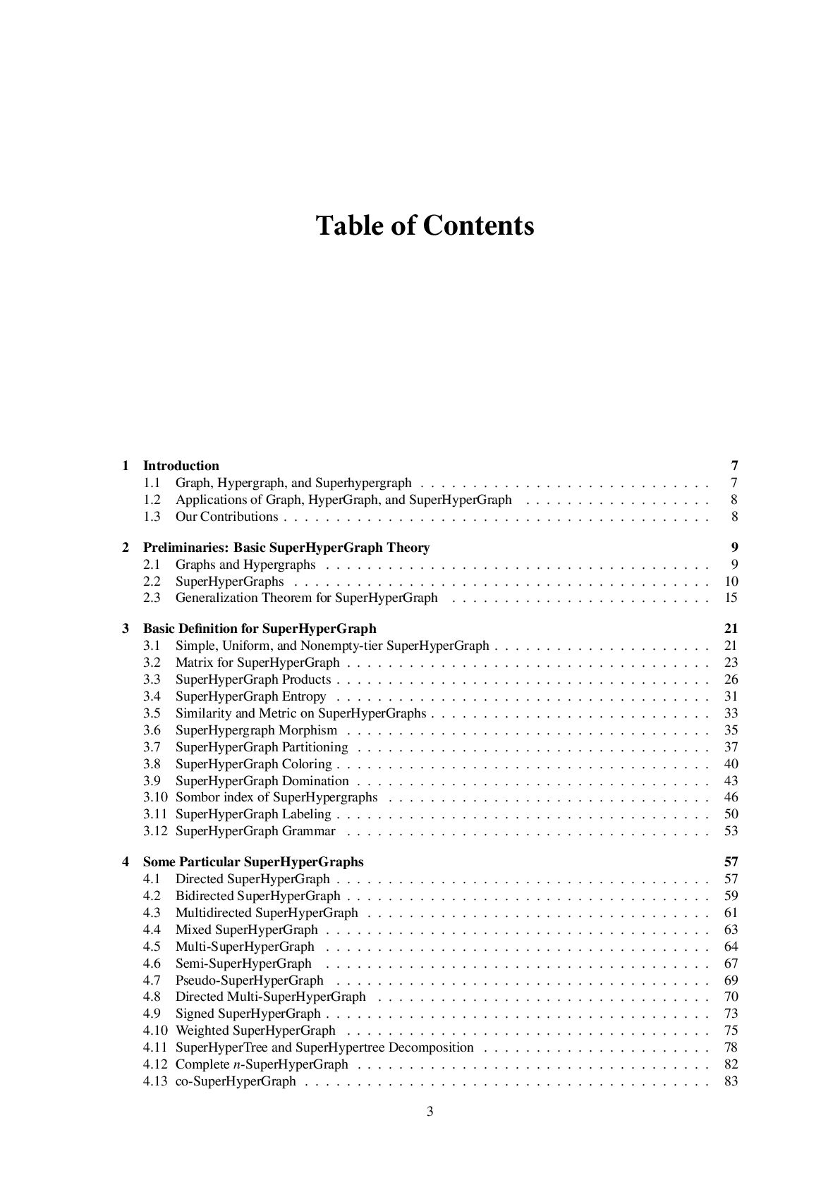
Table of Contents 1 Introduction 7 1.1 Graph, Hypergraph, and
Superhypergraph . . . . . . . . . . . . . . . . . . . . . . . . . . . . 7 1.2 Applications of Graph, HyperGraph, and SuperHyperGraph . . . . . . . . . . . . . . . . . . 8 1.3 Our Contributions . . . . . . . . . . . . . . . . . . . . . . . . . . . . . . . . . . . . . . . . . 8 2 Preliminaries: Basic SuperHyperGraph Theory 9 2.1 Graphs and Hypergraphs . . . . . . . . . . . . . . . . . . . . . . . . . . . . . . . . . . . . . 9 2.2 SuperHyperGraphs . . . . . . . . . . . . . . . . . . . . . . . . . . . . . . . . . . . . . . . . 10 2.3 Generalization Theorem for SuperHyperGraph . . . . . . . . . . . . . . . . . . . . . . . . . 15 3 Basic Definition for SuperHyperGraph 21 3.1 Simple, Uniform, and Nonempty-tier SuperHyperGraph . . . . . . . . . . . . . . . . . . . . . 21 3.2 Matrix for SuperHyperGraph . . . . . . . . . . . . . . . . . . . . . . . . . . . . . . . . . . . 23 3.3 SuperHyperGraph Products . . . . . . . . . . . . . . . . . . . . . . . . . . . . . . . . . . . . 26 3.4 SuperHyperGraph Entropy . . . . . . . . . . . . . . . . . . . . . . . . . . . . . . . . . . . . 31 3.5 Similarity and Metric on SuperHyperGraphs . . . . . . . . . . . . . . . . . . . . . . . . . . . 33 3.6 SuperHypergraph Morphism . . . . . . . . . . . . . . . . . . . . . . . . . . . . . . . . . . . 35 3.7 SuperHyperGraph Partitioning . . . . . . . . . . . . . . . . . . . . . . . . . . . . . . . . . . 37 3.8 SuperHyperGraph Coloring . . . . . . . . . . . . . . . . . . . . . . . . . . . . . . . . . . . . 40 3.9 SuperHyperGraph Domination . . . . . . . . . . . . . . . . . . . . . . . . . . . . . . . . . . 43 3.10 Sombor index of SuperHypergraphs . . . . . . . . . . . . . . . . . . . . . . . . . . . . . . . 46 3.11 SuperHyperGraph Labeling . . . . . . . . . . . . . . . . . . . . . . . . . . . . . . . . . . . . 50 3.12 SuperHyperGraph Grammar . . . . . . . . . . . . . . . . . . . . . . . . . . . . . . . . . . . 53 4 Some Particular SuperHyperGraphs 57 4.1 Directed SuperHyperGraph . . . . . . . . . . . . . . . . . . . . . . . . . . . . . . . . . . . . 57 4.2 Bidirected SuperHyperGraph . . . . . . . . . . . . . . . . . . . . . . . . . . . . . . . . . . . 59 4.3 Multidirected SuperHyperGraph . . . . . . . . . . . . . . . . . . . . . . . . . . . . . . . . . 61 4.4 Mixed SuperHyperGraph . . . . . . . . . . . . . . . . . . . . . . . . . . . . . . . . . . . . . 63 4.5 Multi-SuperHyperGraph . . . . . . . . . . . . . . . . . . . . . . . . . . . . . . . . . . . . . 64 4.6 Semi-SuperHyperGraph . . . . . . . . . . . . . . . . . . . . . . . . . . . . . . . . . . . . . 67 4.7 Pseudo-SuperHyperGraph . . . . . . . . . . . . . . . . . . . . . . . . . . . . . . . . . . . . 69 4.8 Directed Multi-SuperHyperGraph . . . . . . . . . . . . . . . . . . . . . . . . . . . . . . . . 70 4.9 Signed SuperHyperGraph . . . . . . . . . . . . . . . . . . . . . . . . . . . . . . . . . . . . . 73 4.10 Weighted SuperHyperGraph . . . . . . . . . . . . . . . . . . . . . . . . . . . . . . . . . . . 75 4.11 SuperHyperTree and SuperHypertree Decomposition . . . . . . . . . . . . . . . . . . . . . . 78 4.12 Complete 𝑛-SuperHyperGraph . . . . . . . . . . . . . . . . . . . . . . . . . . . . . . . . . . 82 4.13 co-SuperHyperGraph . . . . . . . . . . . . . . . . . . . . . . . . . . . . . . . . . . . . . . . 83 3

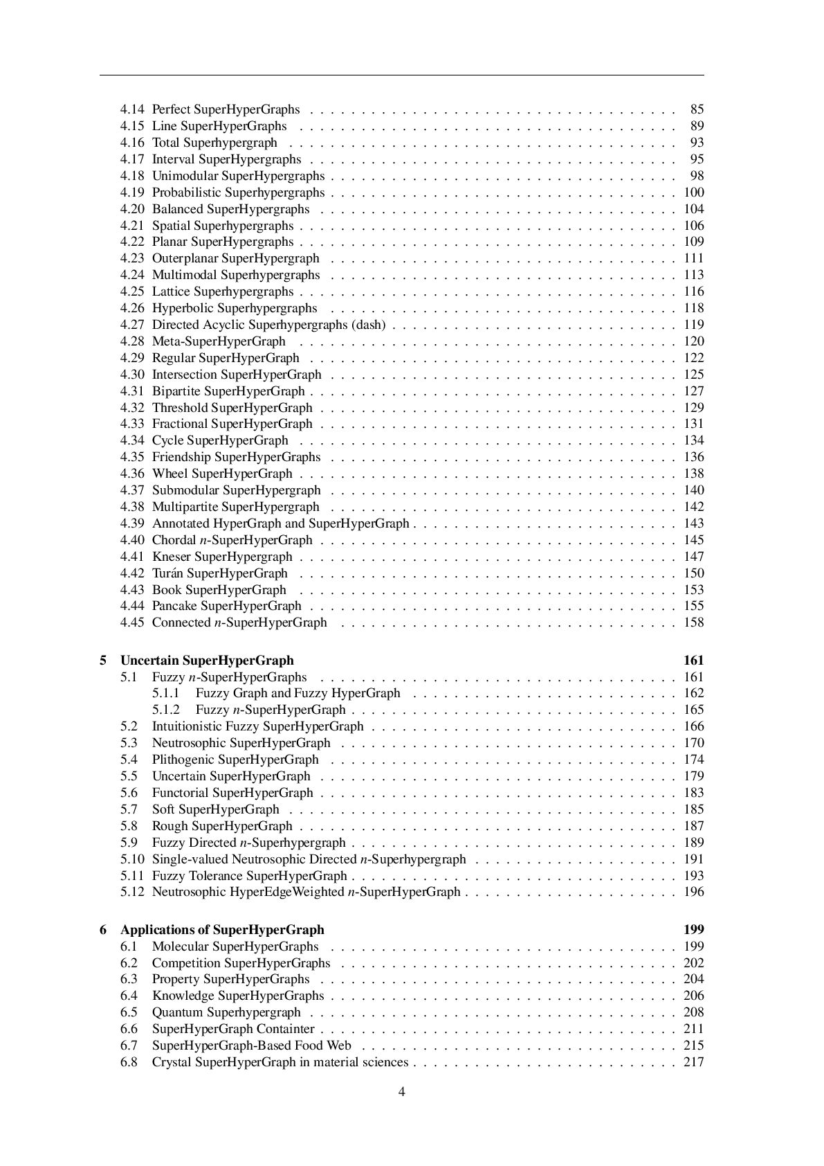
4.14 Perfect SuperHyperGraphs . . . . . . .
. . . . . . . . . . . . . . . . . . . . . . . . . . . . . 85 4.15 Line SuperHyperGraphs . . . . . . . . . . . . . . . . . . . . . . . . . . . . . . . . . . . . . 89 4.16 Total Superhypergraph . . . . . . . . . . . . . . . . . . . . . . . . . . . . . . . . . . . . . . 93 4.17 Interval SuperHypergraphs . . . . . . . . . . . . . . . . . . . . . . . . . . . . . . . . . . . . 95 4.18 Unimodular SuperHypergraphs . . . . . . . . . . . . . . . . . . . . . . . . . . . . . . . . . . 98 4.19 Probabilistic Superhypergraphs . . . . . . . . . . . . . . . . . . . . . . . . . . . . . . . . . . 100 4.20 Balanced SuperHypergraphs . . . . . . . . . . . . . . . . . . . . . . . . . . . . . . . . . . . 104 4.21 Spatial Superhypergraphs . . . . . . . . . . . . . . . . . . . . . . . . . . . . . . . . . . . . . 106 4.22 Planar SuperHypergraphs . . . . . . . . . . . . . . . . . . . . . . . . . . . . . . . . . . . . . 109 4.23 Outerplanar SuperHypergraph . . . . . . . . . . . . . . . . . . . . . . . . . . . . . . . . . . 111 4.24 Multimodal Superhypergraphs . . . . . . . . . . . . . . . . . . . . . . . . . . . . . . . . . . 113 4.25 Lattice Superhypergraphs . . . . . . . . . . . . . . . . . . . . . . . . . . . . . . . . . . . . . 116 4.26 Hyperbolic Superhypergraphs . . . . . . . . . . . . . . . . . . . . . . . . . . . . . . . . . . 118 4.27 Directed Acyclic Superhypergraphs (dash) . . . . . . . . . . . . . . . . . . . . . . . . . . . . 119 4.28 Meta-SuperHyperGraph . . . . . . . . . . . . . . . . . . . . . . . . . . . . . . . . . . . . . 120 4.29 Regular SuperHyperGraph . . . . . . . . . . . . . . . . . . . . . . . . . . . . . . . . . . . . 122 4.30 Intersection SuperHyperGraph . . . . . . . . . . . . . . . . . . . . . . . . . . . . . . . . . . 125 4.31 Bipartite SuperHyperGraph . . . . . . . . . . . . . . . . . . . . . . . . . . . . . . . . . . . . 127 4.32 Threshold SuperHyperGraph . . . . . . . . . . . . . . . . . . . . . . . . . . . . . . . . . . . 129 4.33 Fractional SuperHyperGraph . . . . . . . . . . . . . . . . . . . . . . . . . . . . . . . . . . . 131 4.34 Cycle SuperHyperGraph . . . . . . . . . . . . . . . . . . . . . . . . . . . . . . . . . . . . . 134 4.35 Friendship SuperHyperGraphs . . . . . . . . . . . . . . . . . . . . . . . . . . . . . . . . . . 136 4.36 Wheel SuperHyperGraph . . . . . . . . . . . . . . . . . . . . . . . . . . . . . . . . . . . . . 138 4.37 Submodular SuperHypergraph . . . . . . . . . . . . . . . . . . . . . . . . . . . . . . . . . . 140 4.38 Multipartite SuperHypergraph . . . . . . . . . . . . . . . . . . . . . . . . . . . . . . . . . . 142 4.39 Annotated HyperGraph and SuperHyperGraph . . . . . . . . . . . . . . . . . . . . . . . . . . 143 4.40 Chordal 𝑛-SuperHyperGraph . . . . . . . . . . . . . . . . . . . . . . . . . . . . . . . . . . . 145 4.41 Kneser SuperHypergraph . . . . . . . . . . . . . . . . . . . . . . . . . . . . . . . . . . . . . 147 4.42 Tur´ an SuperHyperGraph . . . . . . . . . . . . . . . . . . . . . . . . . . . . . . . . . . . . . 150 4.43 Book SuperHyperGraph . . . . . . . . . . . . . . . . . . . . . . . . . . . . . . . . . . . . . 153 4.44 Pancake SuperHyperGraph . . . . . . . . . . . . . . . . . . . . . . . . . . . . . . . . . . . . 155 4.45 Connected 𝑛-SuperHyperGraph . . . . . . . . . . . . . . . . . . . . . . . . . . . . . . . . . 158 5 Uncertain SuperHyperGraph 161 5.1 Fuzzy 𝑛-SuperHyperGraphs . . . . . . . . . . . . . . . . . . . . . . . . . . . . . . . . . . . 161 5.1.1 Fuzzy Graph and Fuzzy HyperGraph . . . . . . . . . . . . . . . . . . . . . . . . . . 162 5.1.2 Fuzzy 𝑛-SuperHyperGraph . . . . . . . . . . . . . . . . . . . . . . . . . . . . . . . . 165 5.2 Intuitionistic Fuzzy SuperHyperGraph . . . . . . . . . . . . . . . . . . . . . . . . . . . . . . 166 5.3 Neutrosophic SuperHyperGraph . . . . . . . . . . . . . . . . . . . . . . . . . . . . . . . . . 170 5.4 Plithogenic SuperHyperGraph . . . . . . . . . . . . . . . . . . . . . . . . . . . . . . . . . . 174 5.5 Uncertain SuperHyperGraph . . . . . . . . . . . . . . . . . . . . . . . . . . . . . . . . . . . 179 5.6 Functorial SuperHyperGraph . . . . . . . . . . . . . . . . . . . . . . . . . . . . . . . . . . . 183 5.7 Soft SuperHyperGraph . . . . . . . . . . . . . . . . . . . . . . . . . . . . . . . . . . . . . . 185 5.8 Rough SuperHyperGraph . . . . . . . . . . . . . . . . . . . . . . . . . . . . . . . . . . . . . 187 5.9 Fuzzy Directed 𝑛-Superhypergraph . . . . . . . . . . . . . . . . . . . . . . . . . . . . . . . . 189 5.10 Single-valued Neutrosophic Directed 𝑛-Superhypergraph . . . . . . . . . . . . . . . . . . . . 191 5.11 Fuzzy Tolerance SuperHyperGraph . . . . . . . . . . . . . . . . . . . . . . . . . . . . . . . . 193 5.12 Neutrosophic HyperEdgeWeighted 𝑛-SuperHyperGraph . . . . . . . . . . . . . . . . . . . . . 196 6 Applications of SuperHyperGraph 199 6.1 Molecular SuperHyperGraphs . . . . . . . . . . . . . . . . . . . . . . . . . . . . . . . . . . 199 6.2 Competition SuperHyperGraphs . . . . . . . . . . . . . . . . . . . . . . . . . . . . . . . . . 202 6.3 Property SuperHyperGraphs . . . . . . . . . . . . . . . . . . . . . . . . . . . . . . . . . . . 204 6.4 Knowledge SuperHyperGraphs . . . . . . . . . . . . . . . . . . . . . . . . . . . . . . . . . . 206 6.5 Quantum Superhypergraph . . . . . . . . . . . . . . . . . . . . . . . . . . . . . . . . . . . . 208 6.6 SuperHyperGraph Containter . . . . . . . . . . . . . . . . . . . . . . . . . . . . . . . . . . . 211 6.7 SuperHyperGraph-Based Food Web . . . . . . . . . . . . . . . . . . . . . . . . . . . . . . . 215 6.8 Crystal SuperHyperGraph in material sciences . . . . . . . . . . . . . . . . . . . . . . . . . . 217 4

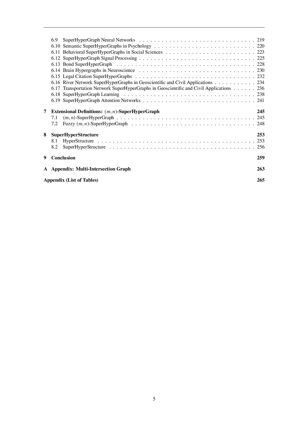
6.9 SuperHyperGraph Neural Networks . . . . . .
. . . . . . . . . . . . . . . . . . . . . . . . . 219 6.10 Semantic SuperHyperGraphs in Psychology . . . . . . . . . . . . . . . . . . . . . . . . . . . 220 6.11 Behavioral SuperHyperGraphs in Social Sciences . . . . . . . . . . . . . . . . . . . . . . . . 223 6.12 SuperHyperGraph Signal Processing . . . . . . . . . . . . . . . . . . . . . . . . . . . . . . . 225 6.13 Bond SuperHyperGraph . . . . . . . . . . . . . . . . . . . . . . . . . . . . . . . . . . . . . 228 6.14 Brain Hypergraphs in Neuroscience . . . . . . . . . . . . . . . . . . . . . . . . . . . . . . . 230 6.15 Legal Citation SuperHyperGraphs . . . . . . . . . . . . . . . . . . . . . . . . . . . . . . . . 232 6.16 River Network SuperHyperGraphs in Geoscientific and Civil Applications . . . . . . . . . . . 234 6.17 Transportation Network SuperHyperGraphs in Geoscientific and Civil Applications . . . . . . 236 6.18 SuperHyperGraph Learning . . . . . . . . . . . . . . . . . . . . . . . . . . . . . . . . . . . 238 6.19 SuperHyperGraph Attention Networks . . . . . . . . . . . . . . . . . . . . . . . . . . . . . . 241 7 Extensional Definitions: (𝑚, 𝑛)-SuperHyperGraph 245 7.1 (𝑚, 𝑛)-SuperHyperGraph . . . . . . . . . . . . . . . . . . . . . . . . . . . . . . . . . . . . . 245 7.2 Fuzzy (𝑚, 𝑛)-SuperHyperGraph . . . . . . . . . . . . . . . . . . . . . . . . . . . . . . . . . 248 8 SuperHyperStructure 253 8.1 HyperStructure . . . . . . . . . . . . . . . . . . . . . . . . . . . . . . . . . . . . . . . . . . 253 8.2 SuperHyperStructure . . . . . . . . . . . . . . . . . . . . . . . . . . . . . . . . . . . . . . . 256 9 Conclusion 259 A Appendix: Multi-Intersection Graph 263 Appendix (List of Tables) 265 5

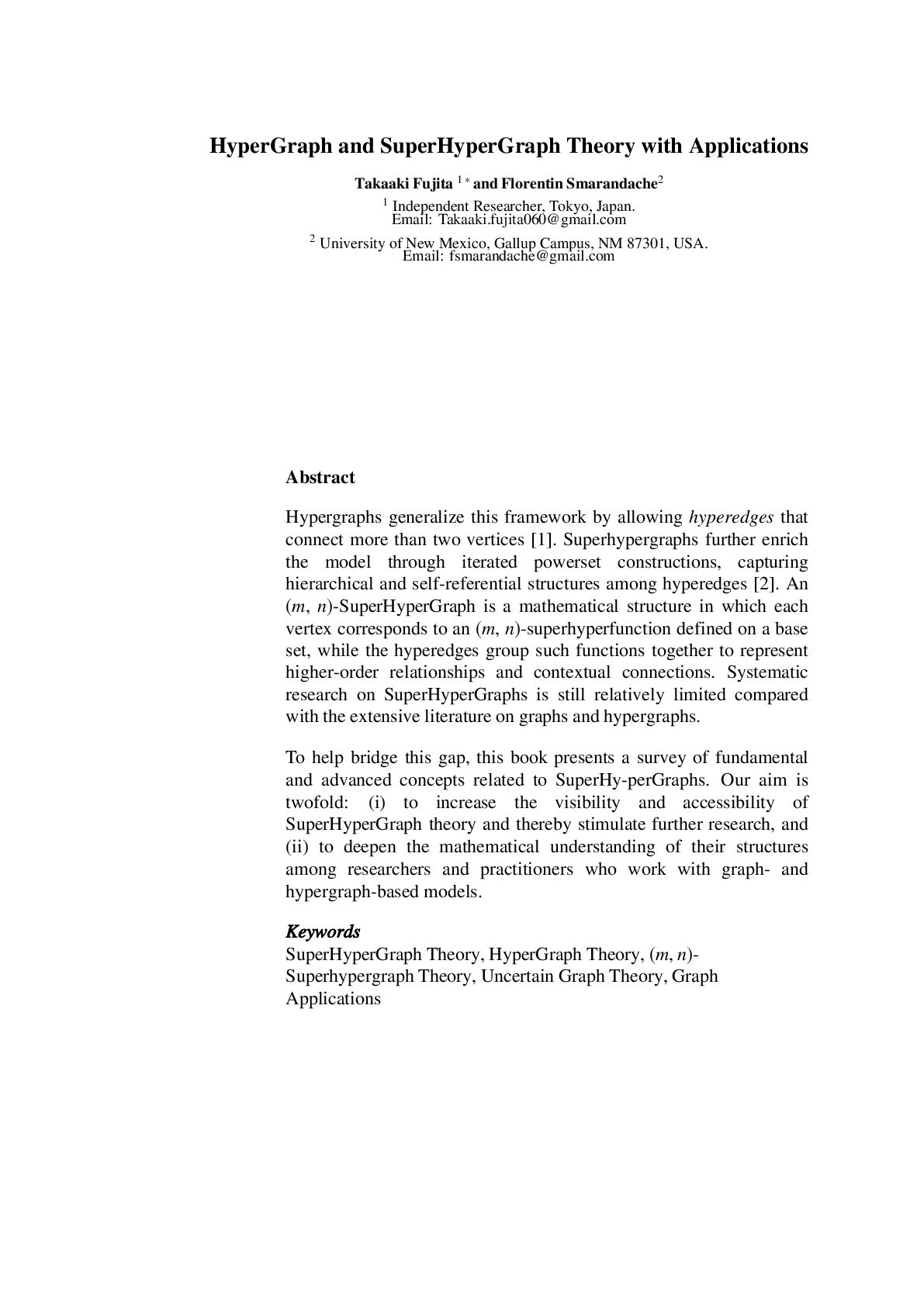
Abstract Hypergraphs generalize this framework by allowing hyperedges that connect
more than two vertices [1]. Superhypergraphs further enrich the model through iterated powerset constructions, capturing hierarchical and self-referential structures among hyperedges [2]. An (𝑚, 𝑛)-SuperHyperGraph is a mathematical structure in which each vertex corresponds to an (𝑚, 𝑛)-superhyperfunction defined on a base set, while the hyperedges group such functions together to represent higher-order relationships and contextual connections. Systematic research on SuperHyperGraphs is still relatively limited compared with the extensive literature on graphs and hypergraphs. To help bridge this gap, this book presents a survey of fundamental and advanced concepts related to SuperHy-perGraphs. Our aim is twofold: (i) to increase the visibility and accessibility of SuperHyperGraph theory and thereby stimulate further research, and (ii) to deepen the mathematical understanding of their structures among researchers and practitioners who work with graph- and hypergraph-based models. Keywords SuperHyperGraph Theory, HyperGraph Theory, (𝑚, 𝑛)- Superhypergraph Theory, Uncertain Graph Theory, Graph Applications HyperGraph and SuperHyperGraph Theory with Applications Takaaki Fujita 1 ∗ and Florentin Smarandache2 1 Independent Researcher, Tokyo, Japan. Email: [email protected] 2 University of New Mexico, Gallup Campus, NM 87301, USA. Email: [email protected]

Chapter 1 Introduction 1.1 Graph, Hypergraph, and Superhypergraph Network modeling
often relies on graphs, where entities are represented by vertices and binary relations are represented by edges [3]. However, classical graphs can be inadequate for describing complex networks in which three or more entities interact simultaneously. Hypergraphs address this limitation by allowing each hyperedge to connect an arbitrary nonempty subset of vertices, thereby capturing higher-order interactions [4]. Despite their expressive power, hypergraphs may still be insufficient for representing layered, nested, and inherently hierarchical relationships that arise in many real-world systems. To bridge this gap, the notion of a SuperHyperGraph was introduced by F. Smarandache. A SuperHyperGraph employs iterative powerset-based constructions to encode nested connectivity patterns and multi-level relations [2,5], and has attracted substantial recent attention [6,7]. Graphs and hypergraphs provide intuitive visual metaphors for complex systems and support a wide range of applications in artificial intelligence, network science, data mining, informatics, chemistry, physics, and beyond [8–11]. By explicitly accommodating hierarchical and multi-level relationships, SuperHyperGraphs offer a robust framework for modeling and analyzing the intricate structures encountered in modern networked data (e.g.. [12–14,14–16]). Table 1.1 summarizes the key distinctions among graphs, hypergraphs, and superhypergraphs. Throughout this book, 𝑛 is taken to be a natural number unless stated otherwise. Table 1.1: Key distinctions among graph, hypergraph, and superhypergraph Concept Notation Edge Type Extension Mechanism Graph [3] 𝐺 = (𝑉, 𝐸) 𝐸 ⊆ {{𝑢, 𝑣} | 𝑢, 𝑣 ∈ 𝑉, 𝑢 ≠ 𝑣} Standard edges connect exactly two vertices. Hypergraph [17] 𝐻 = (𝑉, 𝐸) 𝐸 ⊆ P(𝑉) \ {∅} Hyperedges may join any nonempty subset of vertices. Superhypergraph [2] SHG(𝑛) = (𝑉0,𝑉, 𝐸) 𝑉 ⊆ P𝑛 (𝑉0 ), 𝐸 ⊆ P(𝑉) Applies an 𝑛-fold powerset to capture nested structure. Notation. P(𝑋) = { 𝐴 ⊆ 𝑋} and P0 (𝑋) = 𝑋, P𝑘+1 (𝑋) = P(P𝑘 (𝑋)). Advantages of Using SuperHyperGraphs include several well-known benefits, such as: • Naturally modeling hierarchical structures through iterated powersets. • Representing multiway, multi-level relations within a unified framework. • Containing graphs [3], multi-graphs [18,19], subset-vertex graphs [20–22], hypergraphs [17], supergraph [23], h-model [24], Quasi-SuperHyperGraphs [5], Powerset Graph [25], k-chain free sets [26], johnson [27], kneser graphs [28], and multi-hypergraphs [29] as special (flattened) instances. 7

Chapter 1. Introduction • Supporting rich attribute systems (fuzzy, intuitionstic
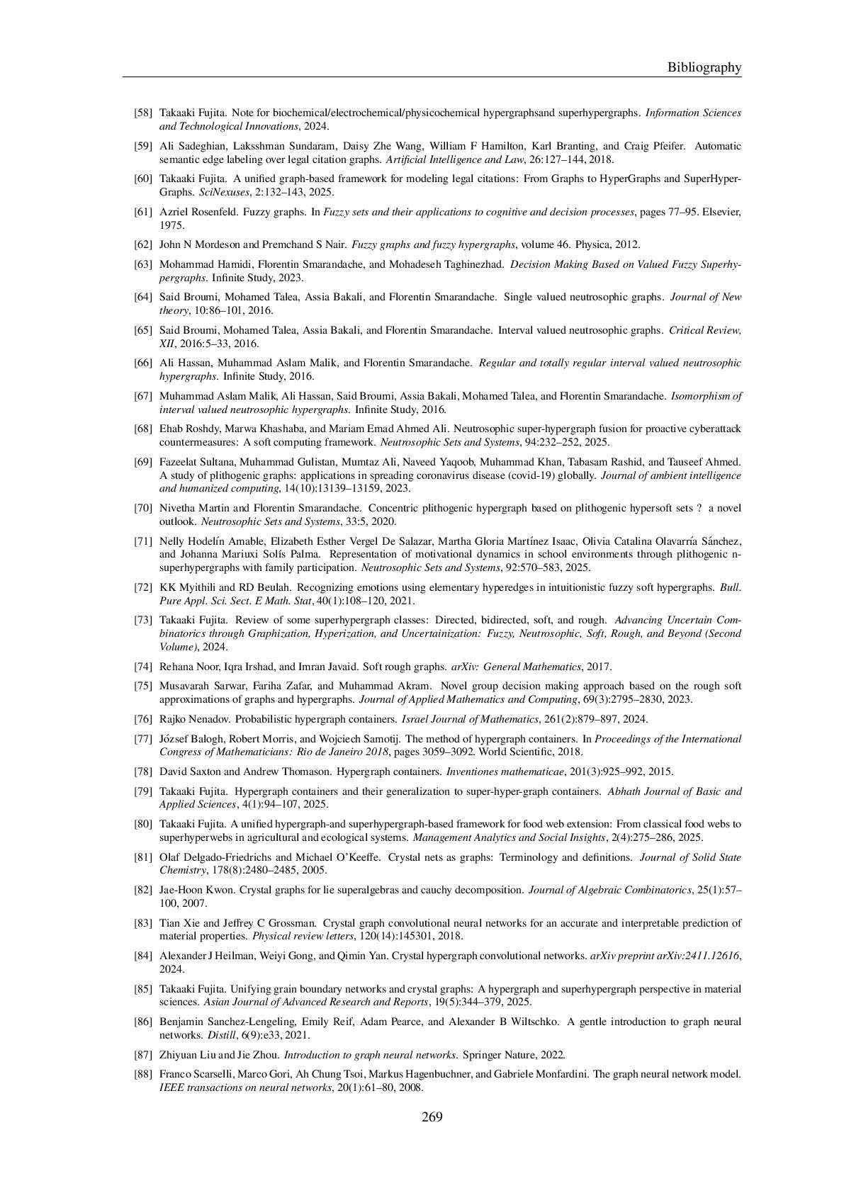
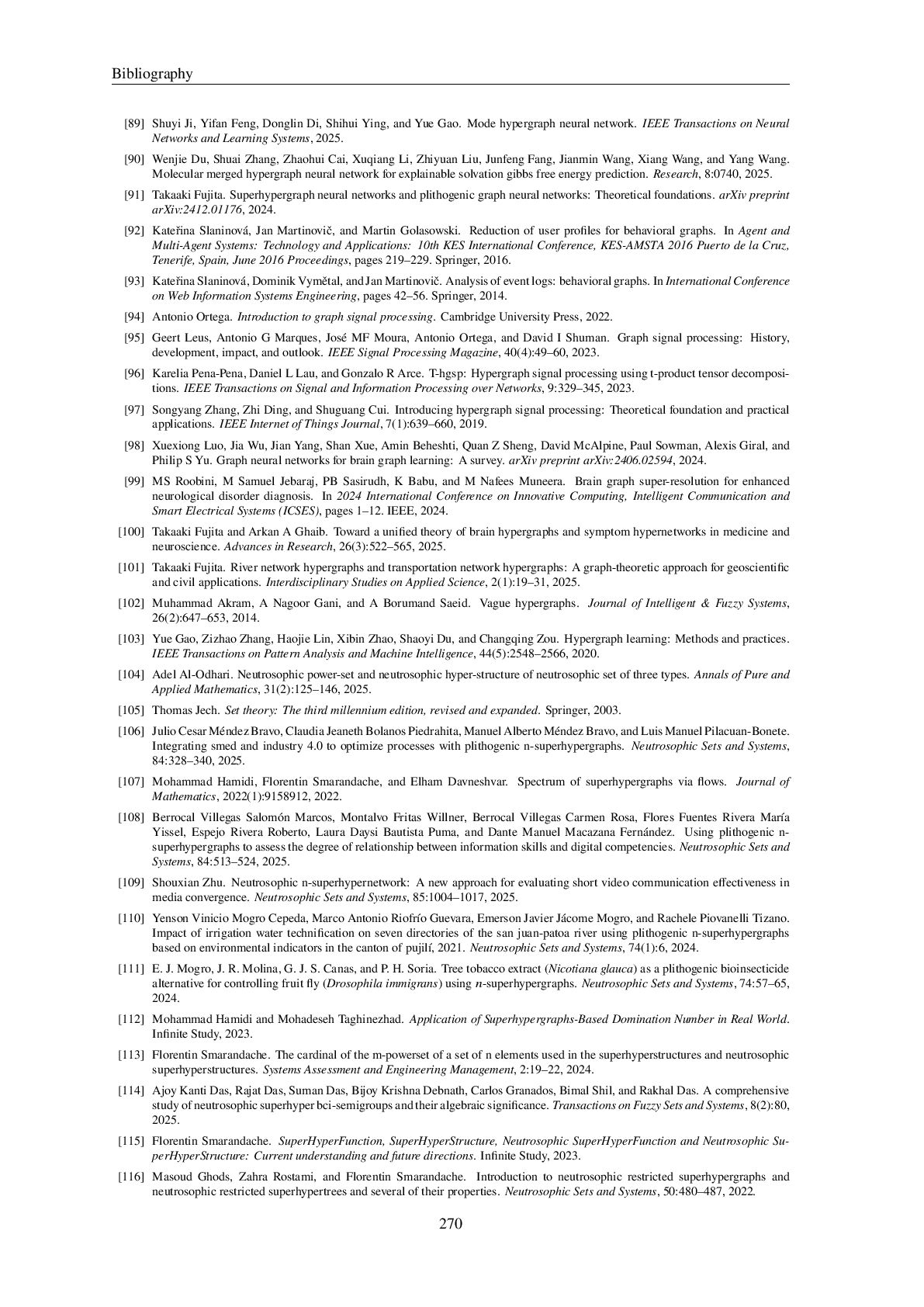
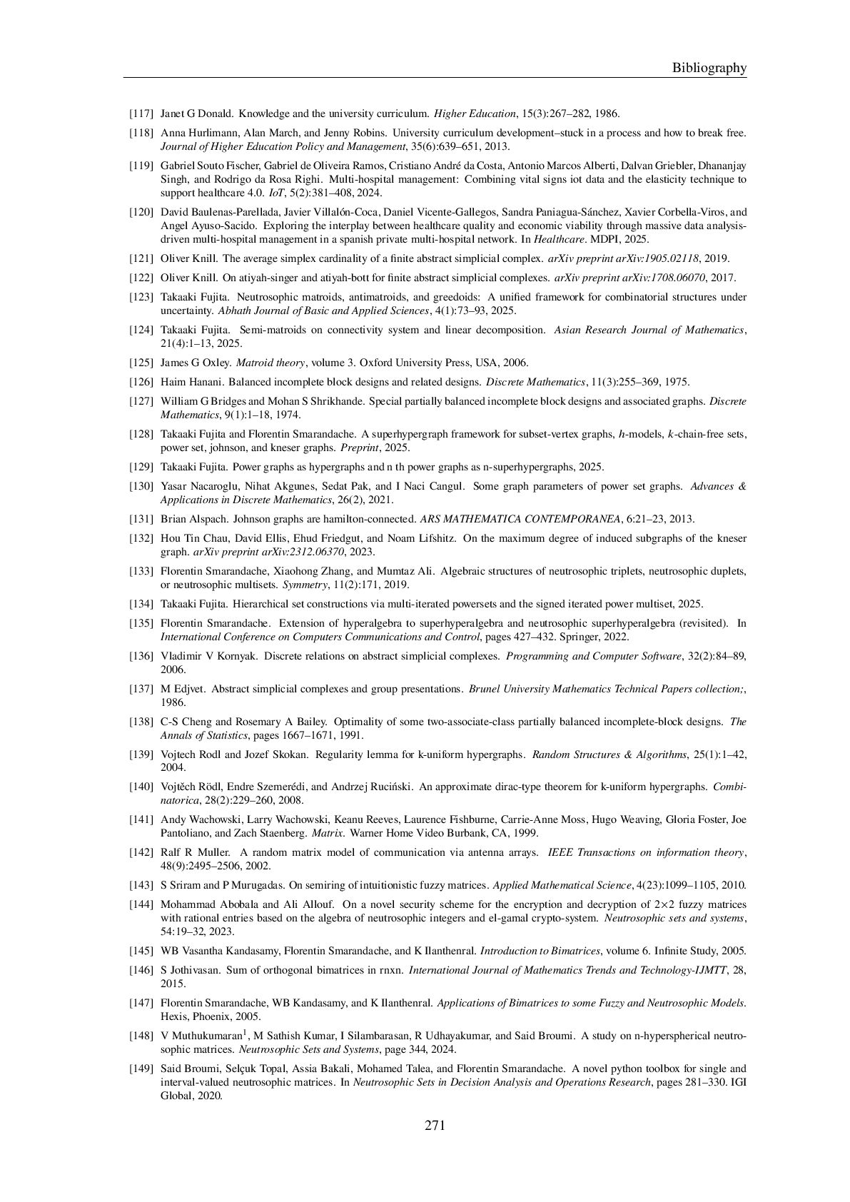
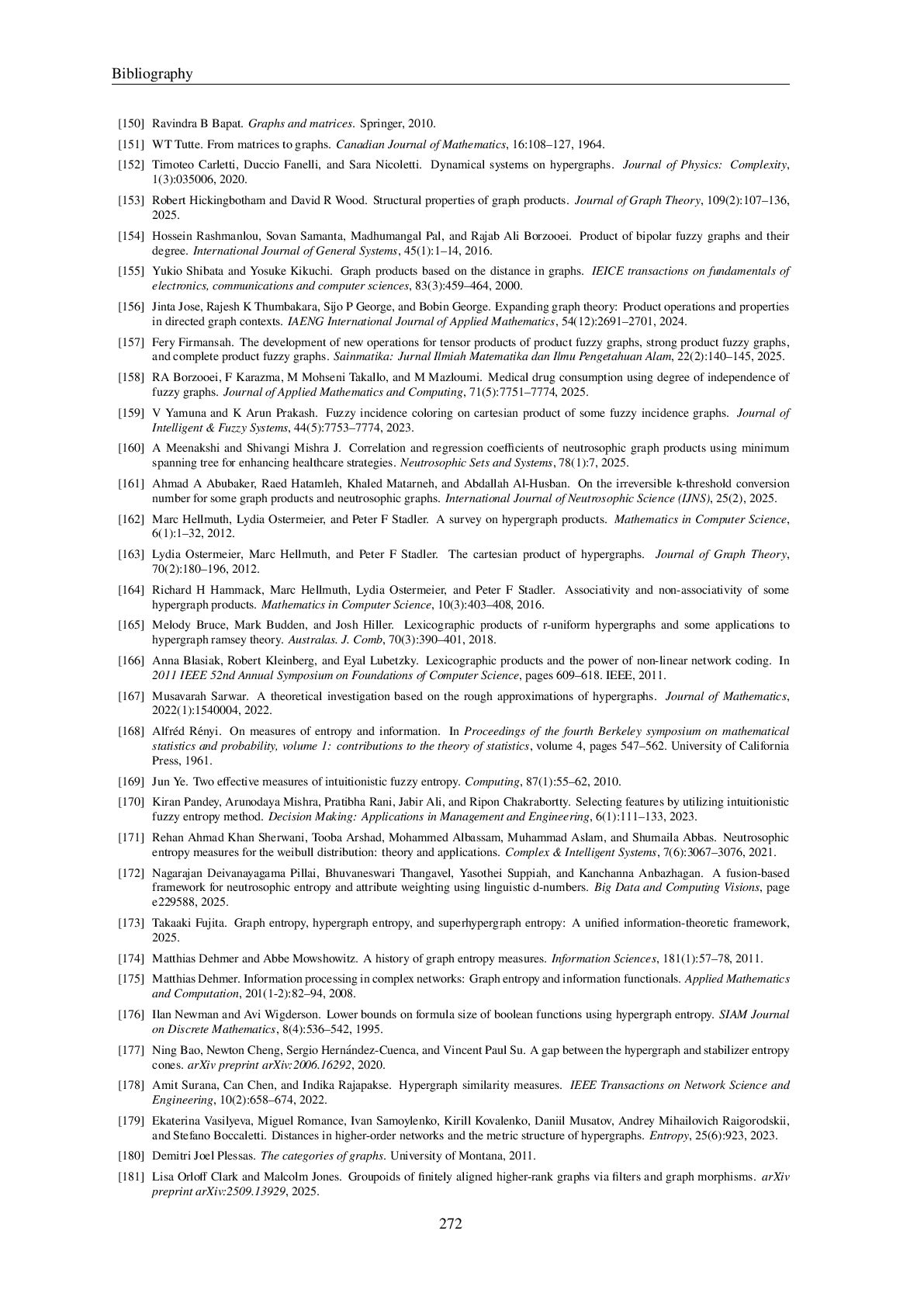
fuzzy, neutrosophic, plithogenic [2]) at every level. • Providing a better fit for real hierarchical systems such as curricula or supply-chain networks. 1.2 Applications of Graph, HyperGraph, and SuperHyperGraph Graph, HyperGraph, and SuperHyperGraph structures have been investigated in a wide range of application domains. Representative examples are summarized in Table 1.2 and 1.3. It should be noted that research on SuperHyperGraphs is still in its early stages, and most existing work remains theoretical at the time of writing. Consequently, future studies are expected to include more practical research supported by computational experiments, machine-learning techniques, and detailed case studies conducted by domain experts. Table 1.2: Applied graph, hypergraph, and superhypergraph models Application domain Graph model HyperGraph model SuperHyperGraph model Generic network Graph HyperGraph SuperHyperGraph Molecular structure Molecular Graph [30] Molecular HyperGraph [31] Molecular SuperHyperGraph [32] Competition / ecology Competition Graph [33] Competition HyperGraph [34] Competition SuperHyperGraph [35] Knowledge / semantics Knowledge Graph [36] Knowledge HyperGraph [37,38] Knowledge SuperHyperGraph [39] Property-based system Property Graph [40] Property HyperGraph [41] Property SuperHyperGraph [41] Semi-structured network SemiGraph [42] SemiHyperGraph [43] Semi-SuperHyperGraph [5] Quantum system Quantum Graph [44,45] Quantum HyperGraph [46] Quantum SuperHyperGraph [47] Semantic relations Semantic Graph [48] Semantic HyperGraph [49] Semantic SuperHyperGraph [50] Bonding Bond Graph [51,52] Bond HyperGraph [53] Bond SuperHyperGraph [53] Chemical reactions Chemical Graph [54] Chemical HyperGraph [55,56] Chemical SuperHyperGraph [57,58] Legal citation network Legal Citation Graph [59] Legal Citation HyperGraph [60] Legal Citation SuperHyperGraph [60] Fuzzy uncertainty Fuzzy Graph [61] Fuzzy HyperGraph [62] Fuzzy SuperHyperGraph [63] Neutrosophic uncertainty Neutrosophic Graph [64,65] Neutrosophic HyperGraph [66,67] Neutrosophic SuperHyperGraph [68] Plithogenic uncertainty Plithogenic Graph [69] Plithogenic HyperGraph [70] Plithogenic SuperHyperGraph [13,71] Soft-set based modeling Soft Graph [72] Soft HyperGraph [72] Soft SuperHyperGraph [73] Rough approximation Rough Graph [74] Rough HyperGraph [75] Rough SuperHyperGraph [73] Table 1.3: Additional applied graph, hypergraph, and superhypergraph models (Part 2) Application domain Graph model HyperGraph model SuperHyperGraph model Higher-order containers Graph Container HyperGraph Container [76–78] SuperHyperGraph Container [79] Ecological food webs Graph-based Food Web Hypergraph-based Food Web [80] SuperHyperGraph-Based Food Web [80] Crystal and lattice structures Crystal Graph [81–83] Crystal HyperGraph [84] Crystal SuperHyperGraph [85] Neural architectures Graph Neural Network [86–88] Hypergraph Neural Network [4, 89, 90] SuperHyperGraph Neural Network [91] Social and behavioral modeling Behavioral Graphs in Social Sciences [92,93] Behavioral HyperGraphs in Social Sciences [50] Behavioral SuperHyperGraphs in So- cial Sciences [50] Signal processing on networks Graph Signal Processing [94,95] Hypergraph Signal Processing [96, 97] SuperHyperGraph Signal Processing [53] Brain connectivity Brain Graphs [98,99] Brain HyperGraphs [100] Brain SuperHyperGraphs [100] River basin and watershed systems River Network Graphs River Network HyperGraphs [101] River Network SuperHyperGraphs [101] Transportation and logistics Transportation Network Graphs Transportation Network Hyper- Graphs [101] Transportation Network SuperHy- perGraphs [101] 1.3 Our Contributions From the above discussion, it is clear that SuperHyperGraphs are highly important for modeling hierarchical and multiway structures. However, systematic research on SuperHyperGraphs remains relatively limited compared with the extensive literature on graphs and hypergraphs. To help bridge this gap, this book provides a survey of fundamental and advanced concepts related to Super- HyperGraphs. Our aim is twofold: (i) to increase the visibility and accessibility of SuperHyperGraph theory and thereby stimulate further research, and (ii) to deepen the mathematical understanding of these structures among researchers and practitioners who work with graph- and hypergraph-based models. This book primarily focuses on theoretical developments. We sincerely hope that further computational experiments and real-world case studies will be carried out by experts in the relevant domains. 8

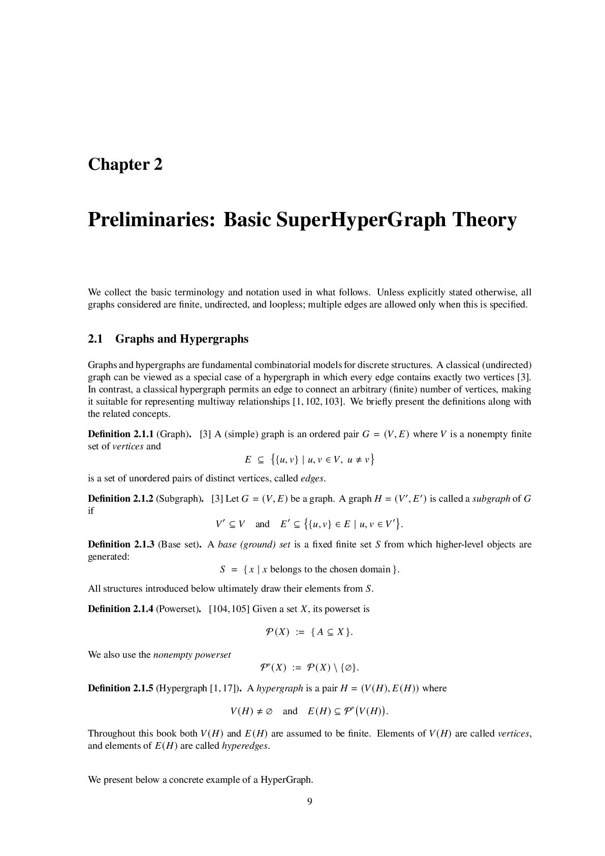
Chapter 2 Preliminaries: Basic SuperHyperGraph Theory We collect the basic
terminology and notation used in what follows. Unless explicitly stated otherwise, all graphs considered are finite, undirected, and loopless; multiple edges are allowed only when this is specified. 2.1 Graphs and Hypergraphs Graphs and hypergraphs are fundamental combinatorial models for discrete structures. A classical (undirected) graph can be viewed as a special case of a hypergraph in which every edge contains exactly two vertices [3]. In contrast, a classical hypergraph permits an edge to connect an arbitrary (finite) number of vertices, making it suitable for representing multiway relationships [1,102,103]. We briefly present the definitions along with the related concepts. Definition 2.1.1 (Graph). [3] A (simple) graph is an ordered pair 𝐺 = (𝑉, 𝐸) where 𝑉 is a nonempty finite set of vertices and 𝐸 ⊆ {𝑢, 𝑣} | 𝑢, 𝑣 ∈ 𝑉, 𝑢 ≠ 𝑣 is a set of unordered pairs of distinct vertices, called edges. Definition 2.1.2 (Subgraph). [3] Let 𝐺 = (𝑉, 𝐸) be a graph. A graph 𝐻 = (𝑉′ , 𝐸′) is called a subgraph of 𝐺 if 𝑉′ ⊆ 𝑉 and 𝐸′ ⊆ {𝑢, 𝑣} ∈ 𝐸 | 𝑢, 𝑣 ∈ 𝑉′ . Definition 2.1.3 (Base set). A base (ground) set is a fixed finite set 𝑆 from which higher-level objects are generated: 𝑆 = { 𝑥 | 𝑥 belongs to the chosen domain }. All structures introduced below ultimately draw their elements from 𝑆. Definition 2.1.4 (Powerset). [104,105] Given a set 𝑋, its powerset is P(𝑋) := { 𝐴 ⊆ 𝑋 }. We also use the nonempty powerset P∗(𝑋) := P(𝑋) \ {∅}. Definition 2.1.5 (Hypergraph [1,17]). A hypergraph is a pair 𝐻 = (𝑉(𝐻), 𝐸(𝐻)) where 𝑉(𝐻) ≠ ∅ and 𝐸(𝐻) ⊆ P∗ 𝑉(𝐻) . Throughout this book both 𝑉(𝐻) and 𝐸(𝐻) are assumed to be finite. Elements of 𝑉(𝐻) are called vertices, and elements of 𝐸(𝐻) are called hyperedges. We present below a concrete example of a HyperGraph. 9

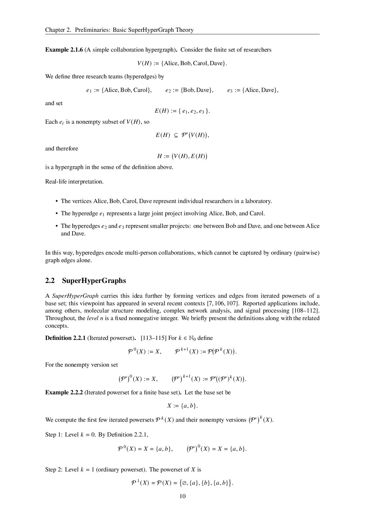
Chapter 2. Preliminaries: Basic SuperHyperGraph Theory Example 2.1.6 (A simple
collaboration hypergraph). Consider the finite set of researchers 𝑉(𝐻) := {Alice, Bob, Carol, Dave}. We define three research teams (hyperedges) by 𝑒1 := {Alice, Bob, Carol}, 𝑒2 := {Bob, Dave}, 𝑒3 := {Alice, Dave}, and set 𝐸(𝐻) := { 𝑒1, 𝑒2, 𝑒3 }. Each 𝑒𝑖 is a nonempty subset of 𝑉(𝐻), so 𝐸(𝐻) ⊆ P∗ 𝑉(𝐻) , and therefore 𝐻 := 𝑉(𝐻), 𝐸(𝐻) is a hypergraph in the sense of the definition above. Real-life interpretation. • The vertices Alice, Bob, Carol, Dave represent individual researchers in a laboratory. • The hyperedge 𝑒1 represents a large joint project involving Alice, Bob, and Carol. • The hyperedges 𝑒2 and 𝑒3 represent smaller projects: one between Bob and Dave, and one between Alice and Dave. In this way, hyperedges encode multi-person collaborations, which cannot be captured by ordinary (pairwise) graph edges alone. 2.2 SuperHyperGraphs A SuperHyperGraph carries this idea further by forming vertices and edges from iterated powersets of a base set; this viewpoint has appeared in several recent contexts [7, 106, 107]. Reported applications include, among others, molecular structure modeling, complex network analysis, and signal processing [108–112]. Throughout, the level 𝑛 is a fixed nonnegative integer. We briefly present the definitions along with the related concepts. Definition 2.2.1 (Iterated powerset). [113–115] For 𝑘 ∈ N0 define P 0(𝑋) := 𝑋, P 𝑘+1(𝑋) := P P 𝑘 (𝑋) . For the nonempty version set P∗ 0(𝑋) := 𝑋, P∗ 𝑘+1(𝑋) := P∗ (P∗)𝑘 (𝑋) . Example 2.2.2 (Iterated powerset for a finite base set). Let the base set be 𝑋 := {𝑎, 𝑏}. We compute the first few iterated powersets P 𝑘 (𝑋) and their nonempty versions P∗ 𝑘 (𝑋). Step 1: Level 𝑘 = 0. By Definition 2.2.1, P 0(𝑋) = 𝑋 = {𝑎, 𝑏}, P∗ 0(𝑋) = 𝑋 = {𝑎, 𝑏}. Step 2: Level 𝑘 = 1 (ordinary powerset). The powerset of 𝑋 is P 1(𝑋) = P(𝑋) = ∅, {𝑎}, {𝑏}, {𝑎, 𝑏} . 10

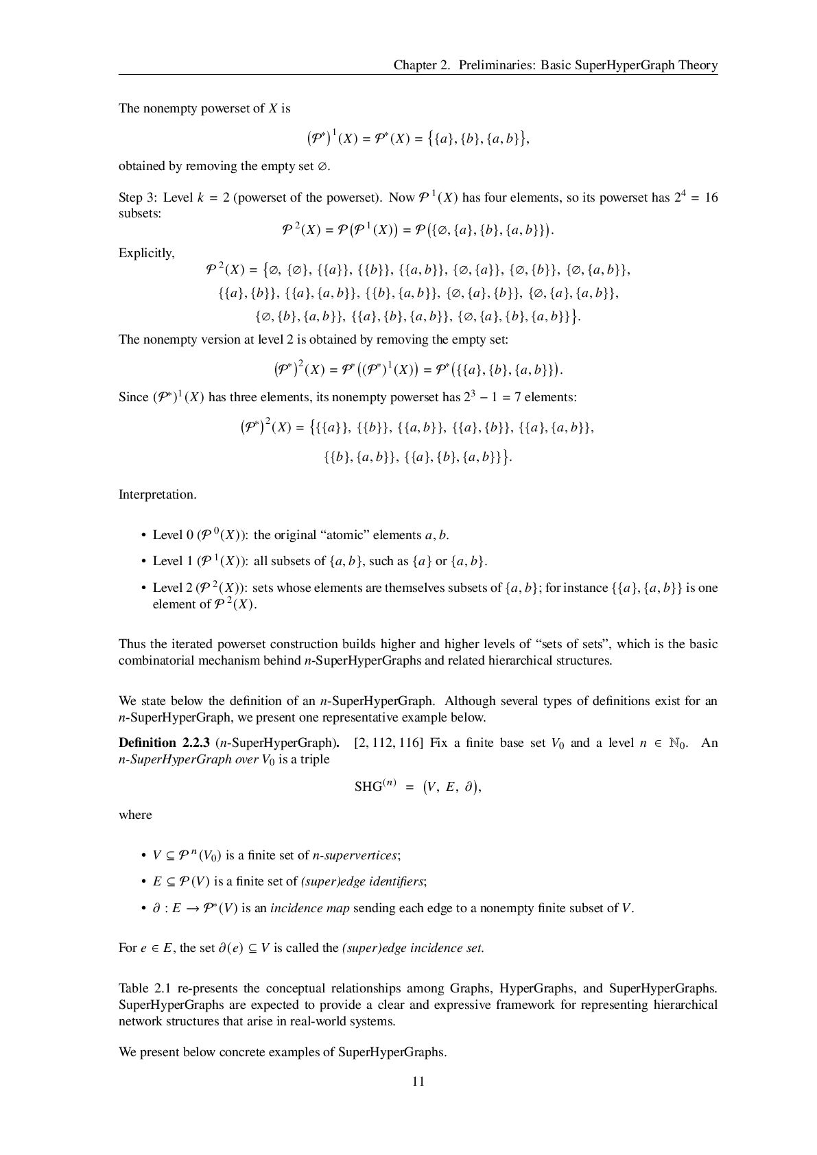
Chapter 2. Preliminaries: Basic SuperHyperGraph Theory The nonempty powerset of
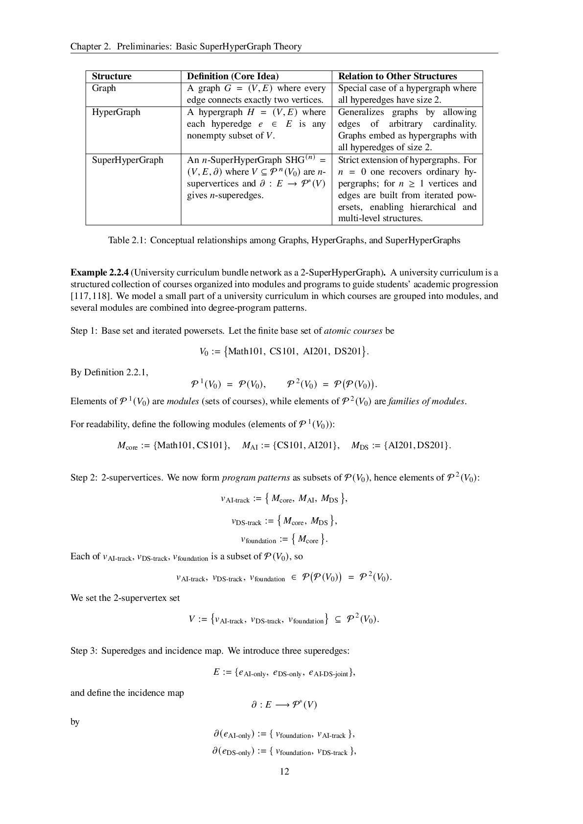
𝑋 is P∗ 1(𝑋) = P∗(𝑋) = {𝑎}, {𝑏}, {𝑎, 𝑏} , obtained by removing the empty set ∅. Step 3: Level 𝑘 = 2 (powerset of the powerset). Now P 1(𝑋) has four elements, so its powerset has 24 = 16 subsets: P 2(𝑋) = P P 1(𝑋) = P {∅, {𝑎}, {𝑏}, {𝑎, 𝑏}} . Explicitly, P 2(𝑋) = ∅, {∅}, {{𝑎}}, {{𝑏}}, {{𝑎, 𝑏}}, {∅, {𝑎}}, {∅, {𝑏}}, {∅, {𝑎, 𝑏}}, {{𝑎}, {𝑏}}, {{𝑎}, {𝑎, 𝑏}}, {{𝑏}, {𝑎, 𝑏}}, {∅, {𝑎}, {𝑏}}, {∅, {𝑎}, {𝑎, 𝑏}}, {∅, {𝑏}, {𝑎, 𝑏}}, {{𝑎}, {𝑏}, {𝑎, 𝑏}}, {∅, {𝑎}, {𝑏}, {𝑎, 𝑏}} . The nonempty version at level 2 is obtained by removing the empty set: P∗ 2(𝑋) = P∗ (P∗)1(𝑋) = P∗ {{𝑎}, {𝑏}, {𝑎, 𝑏}} . Since (P∗)1(𝑋) has three elements, its nonempty powerset has 23 − 1 = 7 elements: P∗ 2(𝑋) = {{𝑎}}, {{𝑏}}, {{𝑎, 𝑏}}, {{𝑎}, {𝑏}}, {{𝑎}, {𝑎, 𝑏}}, {{𝑏}, {𝑎, 𝑏}}, {{𝑎}, {𝑏}, {𝑎, 𝑏}} . Interpretation. • Level 0 (P 0(𝑋)): the original “atomic” elements 𝑎, 𝑏. • Level 1 (P 1(𝑋)): all subsets of {𝑎, 𝑏}, such as {𝑎} or {𝑎, 𝑏}. • Level 2 (P 2(𝑋)): sets whose elements are themselves subsets of {𝑎, 𝑏}; for instance {{𝑎}, {𝑎, 𝑏}} is one element of P 2(𝑋). Thus the iterated powerset construction builds higher and higher levels of “sets of sets”, which is the basic combinatorial mechanism behind 𝑛-SuperHyperGraphs and related hierarchical structures. We state below the definition of an 𝑛-SuperHyperGraph. Although several types of definitions exist for an 𝑛-SuperHyperGraph, we present one representative example below. Definition 2.2.3 (𝑛-SuperHyperGraph). [2, 112, 116] Fix a finite base set 𝑉0 and a level 𝑛 ∈ N0. An 𝑛-SuperHyperGraph over 𝑉0 is a triple SHG(𝑛) = 𝑉, 𝐸, 𝜕 , where • 𝑉 ⊆ P 𝑛(𝑉0 ) is a finite set of 𝑛-supervertices; • 𝐸 ⊆ P(𝑉) is a finite set of (super)edge identifiers; • 𝜕 : 𝐸 → P∗(𝑉) is an incidence map sending each edge to a nonempty finite subset of 𝑉. For 𝑒 ∈ 𝐸, the set 𝜕(𝑒) ⊆ 𝑉 is called the (super)edge incidence set. Table 2.1 re-presents the conceptual relationships among Graphs, HyperGraphs, and SuperHyperGraphs. SuperHyperGraphs are expected to provide a clear and expressive framework for representing hierarchical network structures that arise in real-world systems. We present below concrete examples of SuperHyperGraphs. 11

Chapter 2. Preliminaries: Basic SuperHyperGraph Theory Structure Definition (Core Idea)
Relation to Other Structures Graph A graph 𝐺 = (𝑉, 𝐸) where every edge connects exactly two vertices. Special case of a hypergraph where all hyperedges have size 2. HyperGraph A hypergraph 𝐻 = (𝑉, 𝐸) where each hyperedge 𝑒 ∈ 𝐸 is any nonempty subset of 𝑉. Generalizes graphs by allowing edges of arbitrary cardinality. Graphs embed as hypergraphs with all hyperedges of size 2. SuperHyperGraph An 𝑛-SuperHyperGraph SHG(𝑛) = (𝑉, 𝐸, 𝜕) where 𝑉 ⊆ P 𝑛(𝑉0 ) are 𝑛- supervertices and 𝜕 : 𝐸 → P∗(𝑉) gives 𝑛-superedges. Strict extension of hypergraphs. For 𝑛 = 0 one recovers ordinary hypergraphs; for 𝑛 ≥ 1 vertices and edges are built from iterated powersets, enabling hierarchical and multi-level structures. Table 2.1: Conceptual relationships among Graphs, HyperGraphs, and SuperHyperGraphs Example 2.2.4 (University curriculum bundle network as a 2-SuperHyperGraph). A university curriculum is a structured collection of courses organized into modules and programs to guide students’ academic progression [117,118]. We model a small part of a university curriculum in which courses are grouped into modules, and several modules are combined into degree-program patterns. Step 1: Base set and iterated powersets. Let the finite base set of atomic courses be 𝑉0 := Math101, CS101, AI201, DS201 . By Definition 2.2.1, P 1(𝑉0 ) = P(𝑉0 ), P 2(𝑉0 ) = P P(𝑉0 ) . Elements of P 1(𝑉0 ) are modules (sets of courses), while elements of P 2(𝑉0 ) are families of modules. For readability, define the following modules (elements of P 1(𝑉0 )): 𝑀core := {Math101, CS101}, 𝑀AI := {CS101, AI201}, 𝑀DS := {AI201, DS201}. Step 2: 2-supervertices. We now form program patterns as subsets of P(𝑉0 ), hence elements of P 2(𝑉0 ): 𝑣AI-track := 𝑀core, 𝑀AI, 𝑀DS , 𝑣DS-track := 𝑀core, 𝑀DS , 𝑣foundation := 𝑀core . Each of 𝑣AI-track, 𝑣DS-track, 𝑣foundation is a subset of P(𝑉0 ), so 𝑣AI-track, 𝑣DS-track, 𝑣foundation ∈ P P(𝑉0 ) = P 2(𝑉0 ). We set the 2-supervertex set 𝑉 := 𝑣AI-track, 𝑣DS-track, 𝑣foundation ⊆ P 2(𝑉0 ). Step 3: Superedges and incidence map. We introduce three superedges: 𝐸 := {𝑒AI-only, 𝑒DS-only, 𝑒AI-DS-joint }, and define the incidence map 𝜕 : 𝐸 −→ P∗(𝑉) by 𝜕(𝑒AI-only ) := { 𝑣foundation, 𝑣AI-track }, 𝜕(𝑒DS-only ) := { 𝑣foundation, 𝑣DS-track }, 12

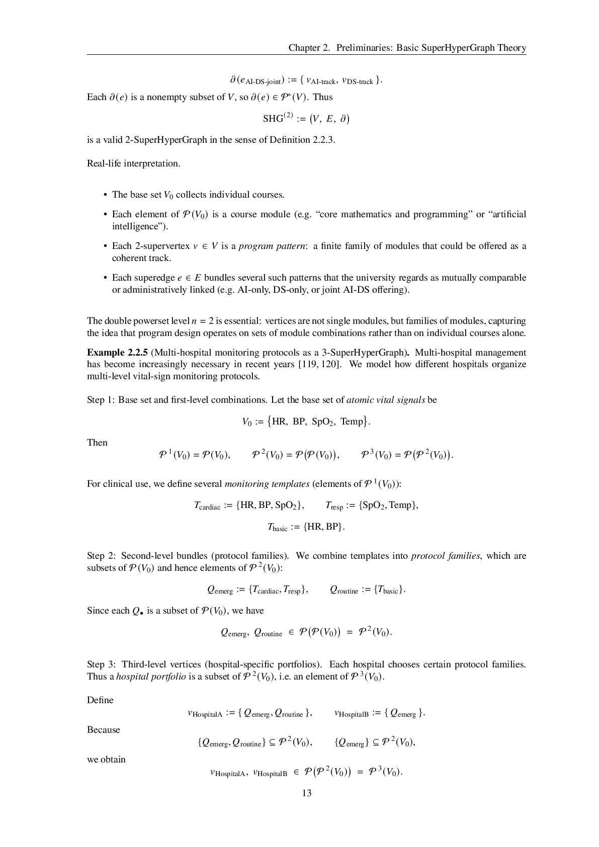
Chapter 2. Preliminaries: Basic SuperHyperGraph Theory 𝜕(𝑒AI-DS-joint ) := {
𝑣AI-track, 𝑣DS-track }. Each 𝜕(𝑒) is a nonempty subset of 𝑉, so 𝜕(𝑒) ∈ P∗(𝑉). Thus SHG(2) := 𝑉, 𝐸, 𝜕 is a valid 2-SuperHyperGraph in the sense of Definition 2.2.3. Real-life interpretation. • The base set 𝑉0 collects individual courses. • Each element of P(𝑉0 ) is a course module (e.g. “core mathematics and programming” or “artificial intelligence”). • Each 2-supervertex 𝑣 ∈ 𝑉 is a program pattern: a finite family of modules that could be offered as a coherent track. • Each superedge 𝑒 ∈ 𝐸 bundles several such patterns that the university regards as mutually comparable or administratively linked (e.g. AI-only, DS-only, or joint AI-DS offering). The double powerset level 𝑛 = 2 is essential: vertices are not single modules, but families of modules, capturing the idea that program design operates on sets of module combinations rather than on individual courses alone. Example 2.2.5 (Multi-hospital monitoring protocols as a 3-SuperHyperGraph). Multi-hospital management has become increasingly necessary in recent years [119, 120]. We model how different hospitals organize multi-level vital-sign monitoring protocols. Step 1: Base set and first-level combinations. Let the base set of atomic vital signals be 𝑉0 := HR, BP, SpO2, Temp . Then P 1(𝑉0 ) = P(𝑉0 ), P 2(𝑉0 ) = P P(𝑉0 ) , P 3(𝑉0 ) = P P 2(𝑉0 ) . For clinical use, we define several monitoring templates (elements of P 1(𝑉0 )): 𝑇cardiac := {HR, BP, SpO2 }, 𝑇resp := {SpO2, Temp}, 𝑇basic := {HR, BP}. Step 2: Second-level bundles (protocol families). We combine templates into protocol families, which are subsets of P(𝑉0 ) and hence elements of P 2(𝑉0 ): 𝑄emerg := {𝑇cardiac,𝑇resp }, 𝑄routine := {𝑇basic }. Since each 𝑄• is a subset of P(𝑉0 ), we have 𝑄emerg, 𝑄routine ∈ P P(𝑉0 ) = P 2(𝑉0 ). Step 3: Third-level vertices (hospital-specific portfolios). Each hospital chooses certain protocol families. Thus a hospital portfolio is a subset of P 2(𝑉0 ), i.e. an element of P 3(𝑉0 ). Define 𝑣HospitalA := { 𝑄emerg, 𝑄routine }, 𝑣HospitalB := { 𝑄emerg }. Because {𝑄emerg, 𝑄routine } ⊆ P 2(𝑉0 ), {𝑄emerg } ⊆ P 2(𝑉0 ), we obtain 𝑣HospitalA, 𝑣HospitalB ∈ P P 2(𝑉0 ) = P 3(𝑉0 ). 13

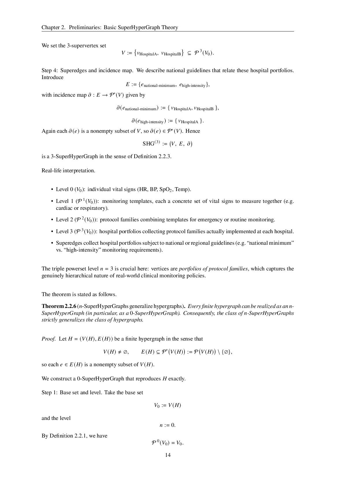
Chapter 2. Preliminaries: Basic SuperHyperGraph Theory We set the 3-supervertex
set 𝑉 := 𝑣HospitalA, 𝑣HospitalB ⊆ P 3(𝑉0 ). Step 4: Superedges and incidence map. We describe national guidelines that relate these hospital portfolios. Introduce 𝐸 := {𝑒national-minimum, 𝑒high-intensity }, with incidence map 𝜕 : 𝐸 → P∗(𝑉) given by 𝜕(𝑒national-minimum ) := { 𝑣HospitalA, 𝑣HospitalB }, 𝜕(𝑒high-intensity ) := { 𝑣HospitalA }. Again each 𝜕(𝑒) is a nonempty subset of 𝑉, so 𝜕(𝑒) ∈ P∗(𝑉). Hence SHG(3) := 𝑉, 𝐸, 𝜕 is a 3-SuperHyperGraph in the sense of Definition 2.2.3. Real-life interpretation. • Level 0 (𝑉0): individual vital signs (HR, BP, SpO2, Temp). • Level 1 (P 1(𝑉0 )): monitoring templates, each a concrete set of vital signs to measure together (e.g. cardiac or respiratory). • Level 2 (P 2(𝑉0 )): protocol families combining templates for emergency or routine monitoring. • Level 3 (P 3(𝑉0 )): hospital portfolios collecting protocol families actually implemented at each hospital. • Superedges collect hospital portfolios subject to national or regional guidelines (e.g. “national minimum” vs. “high-intensity” monitoring requirements). The triple powerset level 𝑛 = 3 is crucial here: vertices are portfolios of protocol families, which captures the genuinely hierarchical nature of real-world clinical monitoring policies. The theorem is stated as follows. Theorem 2.2.6 (𝑛-SuperHyperGraphs generalize hypergraphs). Every finite hypergraph can be realized as an 𝑛- SuperHyperGraph (in particular, as a 0-SuperHyperGraph). Consequently, the class of 𝑛-SuperHyperGraphs strictly generalizes the class of hypergraphs. Proof. Let 𝐻 = (𝑉(𝐻), 𝐸(𝐻)) be a finite hypergraph in the sense that 𝑉(𝐻) ≠ ∅, 𝐸(𝐻) ⊆ P∗ 𝑉(𝐻) := P 𝑉(𝐻) \ {∅}, so each 𝑒 ∈ 𝐸(𝐻) is a nonempty subset of 𝑉(𝐻). We construct a 0-SuperHyperGraph that reproduces 𝐻 exactly. Step 1: Base set and level. Take the base set 𝑉0 := 𝑉(𝐻) and the level 𝑛 := 0. By Definition 2.2.1, we have P 0(𝑉0 ) = 𝑉0. 14

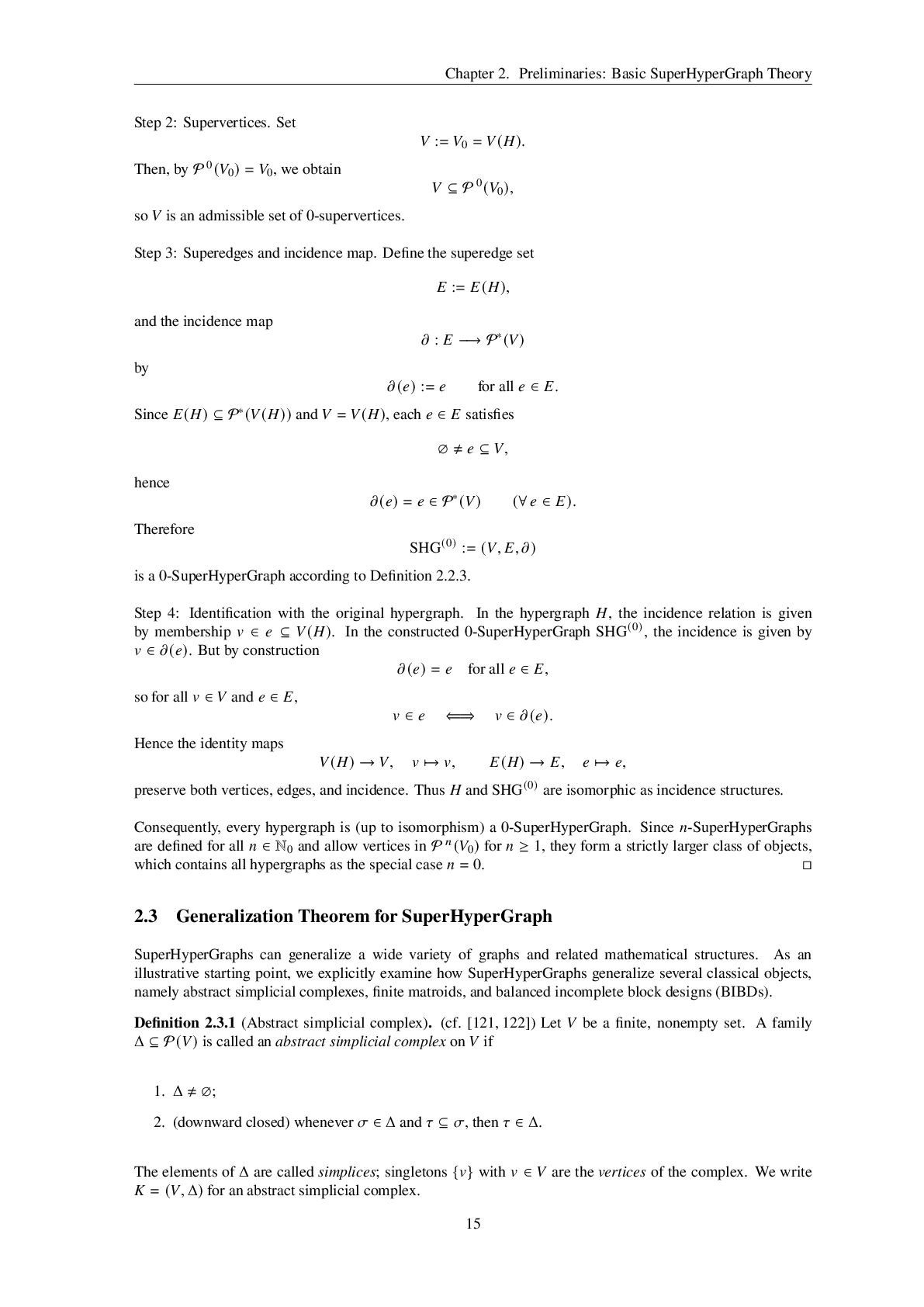
Chapter 2. Preliminaries: Basic SuperHyperGraph Theory Step 2: Supervertices. Set
𝑉 := 𝑉0 = 𝑉(𝐻). Then, by P 0(𝑉0 ) = 𝑉0, we obtain 𝑉 ⊆ P 0(𝑉0 ), so 𝑉 is an admissible set of 0-supervertices. Step 3: Superedges and incidence map. Define the superedge set 𝐸 := 𝐸(𝐻), and the incidence map 𝜕 : 𝐸 −→ P∗(𝑉) by 𝜕(𝑒) := 𝑒 for all 𝑒 ∈ 𝐸. Since 𝐸(𝐻) ⊆ P∗(𝑉(𝐻)) and 𝑉 = 𝑉(𝐻), each 𝑒 ∈ 𝐸 satisfies ∅ ≠ 𝑒 ⊆ 𝑉, hence 𝜕(𝑒) = 𝑒 ∈ P∗(𝑉) (∀ 𝑒 ∈ 𝐸). Therefore SHG(0) := (𝑉, 𝐸, 𝜕) is a 0-SuperHyperGraph according to Definition 2.2.3. Step 4: Identification with the original hypergraph. In the hypergraph 𝐻, the incidence relation is given by membership 𝑣 ∈ 𝑒 ⊆ 𝑉(𝐻). In the constructed 0-SuperHyperGraph SHG(0), the incidence is given by 𝑣 ∈ 𝜕(𝑒). But by construction 𝜕(𝑒) = 𝑒 for all 𝑒 ∈ 𝐸, so for all 𝑣 ∈ 𝑉 and 𝑒 ∈ 𝐸, 𝑣 ∈ 𝑒 ⇐⇒ 𝑣 ∈ 𝜕(𝑒). Hence the identity maps 𝑉(𝐻) → 𝑉, 𝑣 ↦→ 𝑣, 𝐸(𝐻) → 𝐸, 𝑒 ↦→ 𝑒, preserve both vertices, edges, and incidence. Thus 𝐻 and SHG(0) are isomorphic as incidence structures. Consequently, every hypergraph is (up to isomorphism) a 0-SuperHyperGraph. Since 𝑛-SuperHyperGraphs are defined for all 𝑛 ∈ N0 and allow vertices in P 𝑛(𝑉0 ) for 𝑛 ≥ 1, they form a strictly larger class of objects, which contains all hypergraphs as the special case 𝑛 = 0. □ 2.3 Generalization Theorem for SuperHyperGraph SuperHyperGraphs can generalize a wide variety of graphs and related mathematical structures. As an illustrative starting point, we explicitly examine how SuperHyperGraphs generalize several classical objects, namely abstract simplicial complexes, finite matroids, and balanced incomplete block designs (BIBDs). Definition 2.3.1 (Abstract simplicial complex). (cf. [121, 122]) Let 𝑉 be a finite, nonempty set. A family Δ ⊆ P(𝑉) is called an abstract simplicial complex on 𝑉 if 1. Δ ≠ ∅; 2. (downward closed) whenever 𝜎 ∈ Δ and 𝜏 ⊆ 𝜎, then 𝜏 ∈ Δ. The elements of Δ are called simplices; singletons {𝑣} with 𝑣 ∈ 𝑉 are the vertices of the complex. We write 𝐾 = (𝑉, Δ) for an abstract simplicial complex. 15

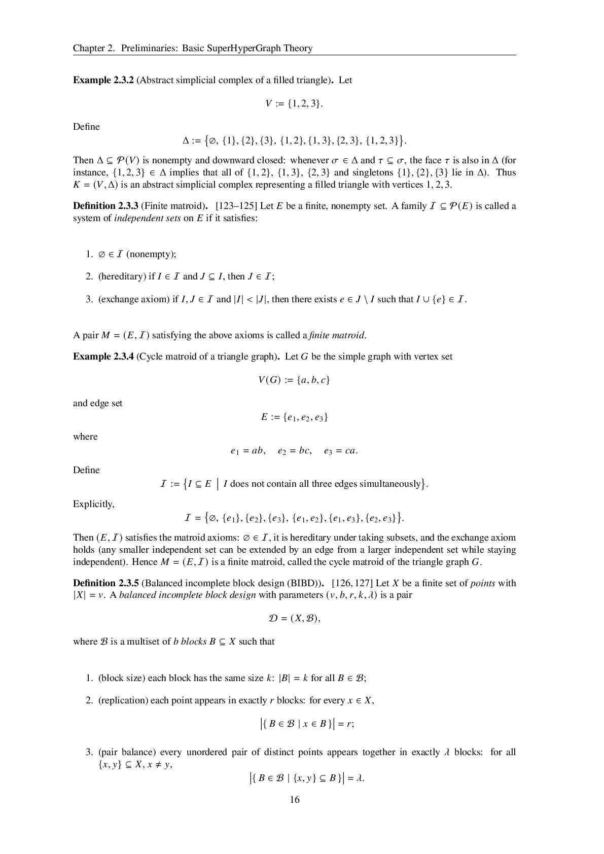
Chapter 2. Preliminaries: Basic SuperHyperGraph Theory Example 2.3.2 (Abstract simplicial
complex of a filled triangle). Let 𝑉 := {1, 2, 3}. Define Δ := ∅, {1}, {2}, {3}, {1, 2}, {1, 3}, {2, 3}, {1, 2, 3} . Then Δ ⊆ P(𝑉) is nonempty and downward closed: whenever 𝜎 ∈ Δ and 𝜏 ⊆ 𝜎, the face 𝜏 is also in Δ (for instance, {1, 2, 3} ∈ Δ implies that all of {1, 2}, {1, 3}, {2, 3} and singletons {1}, {2}, {3} lie in Δ). Thus 𝐾 = (𝑉, Δ) is an abstract simplicial complex representing a filled triangle with vertices 1, 2, 3. Definition 2.3.3 (Finite matroid). [123–125] Let 𝐸 be a finite, nonempty set. A family I ⊆ P(𝐸) is called a system of independent sets on 𝐸 if it satisfies: 1. ∅ ∈ I (nonempty); 2. (hereditary) if 𝐼 ∈ I and 𝐽 ⊆ 𝐼, then 𝐽 ∈ I; 3. (exchange axiom) if 𝐼, 𝐽 ∈ I and |𝐼| < |𝐽|, then there exists 𝑒 ∈ 𝐽 \ 𝐼 such that 𝐼 ∪ {𝑒} ∈ I. A pair 𝑀 = (𝐸, I) satisfying the above axioms is called a finite matroid. Example 2.3.4 (Cycle matroid of a triangle graph). Let 𝐺 be the simple graph with vertex set 𝑉(𝐺) := {𝑎, 𝑏, 𝑐} and edge set 𝐸 := {𝑒1, 𝑒2, 𝑒3 } where 𝑒1 = 𝑎𝑏, 𝑒2 = 𝑏𝑐, 𝑒3 = 𝑐𝑎. Define I := 𝐼 ⊆ 𝐸 𝐼 does not contain all three edges simultaneously . Explicitly, I = ∅, {𝑒1 }, {𝑒2 }, {𝑒3 }, {𝑒1, 𝑒2 }, {𝑒1, 𝑒3 }, {𝑒2, 𝑒3 } . Then (𝐸, I) satisfies the matroid axioms: ∅ ∈ I, it is hereditary under taking subsets, and the exchange axiom holds (any smaller independent set can be extended by an edge from a larger independent set while staying independent). Hence 𝑀 = (𝐸, I) is a finite matroid, called the cycle matroid of the triangle graph 𝐺. Definition 2.3.5 (Balanced incomplete block design (BIBD)). [126,127] Let 𝑋 be a finite set of points with |𝑋| = 𝑣. A balanced incomplete block design with parameters (𝑣, 𝑏, 𝑟, 𝑘, 𝜆) is a pair D = (𝑋, B), where B is a multiset of 𝑏 blocks 𝐵 ⊆ 𝑋 such that 1. (block size) each block has the same size 𝑘: |𝐵| = 𝑘 for all 𝐵 ∈ B; 2. (replication) each point appears in exactly 𝑟 blocks: for every 𝑥 ∈ 𝑋, { 𝐵 ∈ B | 𝑥 ∈ 𝐵 } = 𝑟; 3. (pair balance) every unordered pair of distinct points appears together in exactly 𝜆 blocks: for all {𝑥, 𝑦} ⊆ 𝑋, 𝑥 ≠ 𝑦, { 𝐵 ∈ B | {𝑥, 𝑦} ⊆ 𝐵 } = 𝜆. 16

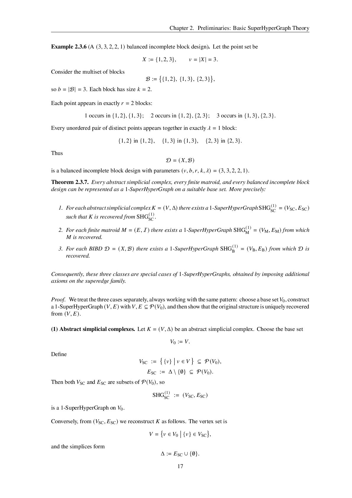
Chapter 2. Preliminaries: Basic SuperHyperGraph Theory Example 2.3.6 (A (3,
3, 2, 2, 1) balanced incomplete block design). Let the point set be 𝑋 := {1, 2, 3}, 𝑣 = |𝑋| = 3. Consider the multiset of blocks B := {1, 2}, {1, 3}, {2, 3} , so 𝑏 = |B| = 3. Each block has size 𝑘 = 2. Each point appears in exactly 𝑟 = 2 blocks: 1 occurs in {1, 2}, {1, 3}; 2 occurs in {1, 2}, {2, 3}; 3 occurs in {1, 3}, {2, 3}. Every unordered pair of distinct points appears together in exactly 𝜆 = 1 block: {1, 2} in {1, 2}, {1, 3} in {1, 3}, {2, 3} in {2, 3}. Thus D = (𝑋, B) is a balanced incomplete block design with parameters (𝑣, 𝑏, 𝑟, 𝑘, 𝜆) = (3, 3, 2, 2, 1). Theorem 2.3.7. Every abstract simplicial complex, every finite matroid, and every balanced incomplete block design can be represented as a 1-SuperHyperGraph on a suitable base set. More precisely: 1. For each abstract simplicialcomplex 𝐾 = (𝑉, Δ) there exists a1-SuperHyperGraphSHG(1) SC = (𝑉SC, 𝐸SC ) such that 𝐾 is recovered from SHG(1) SC . 2. For each finite matroid 𝑀 = (𝐸, I) there exists a 1-SuperHyperGraph SHG(1) M = (𝑉M, 𝐸M ) from which 𝑀 is recovered. 3. For each BIBD D = (𝑋, B) there exists a 1-SuperHyperGraph SHG(1) B = (𝑉B, 𝐸B ) from which D is recovered. Consequently, these three classes are special cases of 1-SuperHyperGraphs, obtained by imposing additional axioms on the superedge family. Proof. We treat the three cases separately, always working with the same pattern: choose a base set𝑉0, construct a 1-SuperHyperGraph (𝑉, 𝐸) with𝑉, 𝐸 ⊆ P(𝑉0 ), and then show that the original structure is uniquely recovered from (𝑉, 𝐸). (1) Abstract simplicial complexes. Let 𝐾 = (𝑉, Δ) be an abstract simplicial complex. Choose the base set 𝑉0 := 𝑉. Define 𝑉SC := {𝑣} 𝑣 ∈ 𝑉 ⊆ P(𝑉0 ), 𝐸SC := Δ \ {∅} ⊆ P(𝑉0 ). Then both 𝑉SC and 𝐸SC are subsets of P(𝑉0 ), so SHG(1) SC := (𝑉SC, 𝐸SC ) is a 1-SuperHyperGraph on 𝑉0. Conversely, from (𝑉SC, 𝐸SC ) we reconstruct 𝐾 as follows. The vertex set is 𝑉 = 𝑣 ∈ 𝑉0 {𝑣} ∈ 𝑉SC , and the simplices form Δ := 𝐸SC ∪ {∅}. 17

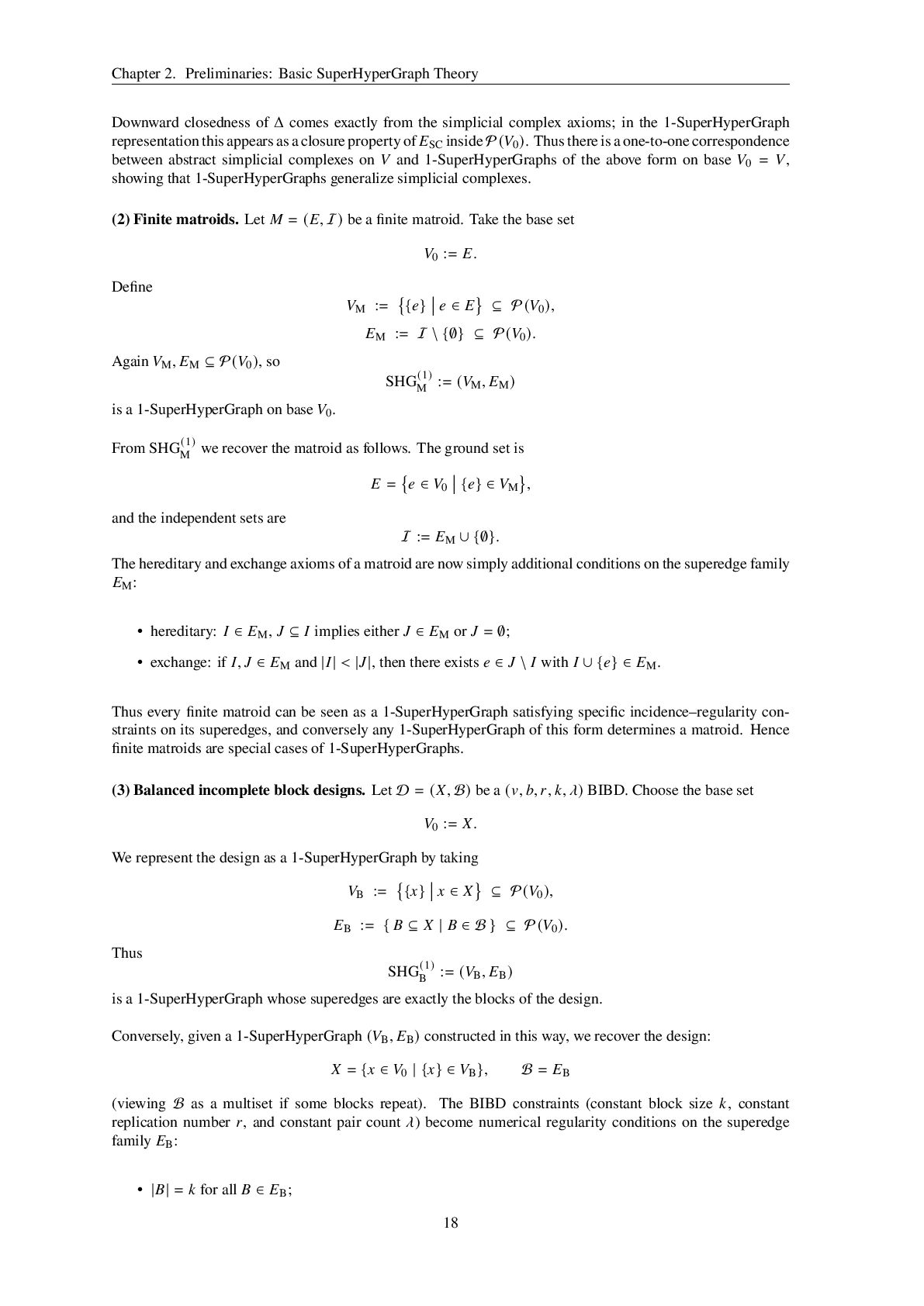
Chapter 2. Preliminaries: Basic SuperHyperGraph Theory Downward closedness of Δ
comes exactly from the simplicial complex axioms; in the 1-SuperHyperGraph representation this appears as a closure property of 𝐸SC inside P(𝑉0 ). Thus there is a one-to-one correspondence between abstract simplicial complexes on 𝑉 and 1-SuperHyperGraphs of the above form on base 𝑉0 = 𝑉, showing that 1-SuperHyperGraphs generalize simplicial complexes. (2) Finite matroids. Let 𝑀 = (𝐸, I) be a finite matroid. Take the base set 𝑉0 := 𝐸. Define 𝑉M := {𝑒} 𝑒 ∈ 𝐸 ⊆ P(𝑉0 ), 𝐸M := I \ {∅} ⊆ P(𝑉0 ). Again 𝑉M, 𝐸M ⊆ P(𝑉0 ), so SHG(1) M := (𝑉M, 𝐸M ) is a 1-SuperHyperGraph on base 𝑉0. From SHG(1) M we recover the matroid as follows. The ground set is 𝐸 = 𝑒 ∈ 𝑉0 {𝑒} ∈ 𝑉M , and the independent sets are I := 𝐸M ∪ {∅}. The hereditary and exchange axioms of a matroid are now simply additional conditions on the superedge family 𝐸M: • hereditary: 𝐼 ∈ 𝐸M, 𝐽 ⊆ 𝐼 implies either 𝐽 ∈ 𝐸M or 𝐽 = ∅; • exchange: if 𝐼, 𝐽 ∈ 𝐸M and |𝐼| < |𝐽|, then there exists 𝑒 ∈ 𝐽 \ 𝐼 with 𝐼 ∪ {𝑒} ∈ 𝐸M. Thus every finite matroid can be seen as a 1-SuperHyperGraph satisfying specific incidence–regularity constraints on its superedges, and conversely any 1-SuperHyperGraph of this form determines a matroid. Hence finite matroids are special cases of 1-SuperHyperGraphs. (3) Balanced incomplete block designs. Let D = (𝑋, B) be a (𝑣, 𝑏, 𝑟, 𝑘, 𝜆) BIBD. Choose the base set 𝑉0 := 𝑋. We represent the design as a 1-SuperHyperGraph by taking 𝑉B := {𝑥} 𝑥 ∈ 𝑋 ⊆ P(𝑉0 ), 𝐸B := { 𝐵 ⊆ 𝑋 | 𝐵 ∈ B } ⊆ P(𝑉0 ). Thus SHG(1) B := (𝑉B, 𝐸B ) is a 1-SuperHyperGraph whose superedges are exactly the blocks of the design. Conversely, given a 1-SuperHyperGraph (𝑉B, 𝐸B ) constructed in this way, we recover the design: 𝑋 = {𝑥 ∈ 𝑉0 | {𝑥} ∈ 𝑉B }, B = 𝐸B (viewing B as a multiset if some blocks repeat). The BIBD constraints (constant block size 𝑘, constant replication number 𝑟, and constant pair count 𝜆) become numerical regularity conditions on the superedge family 𝐸B: • |𝐵| = 𝑘 for all 𝐵 ∈ 𝐸B; 18

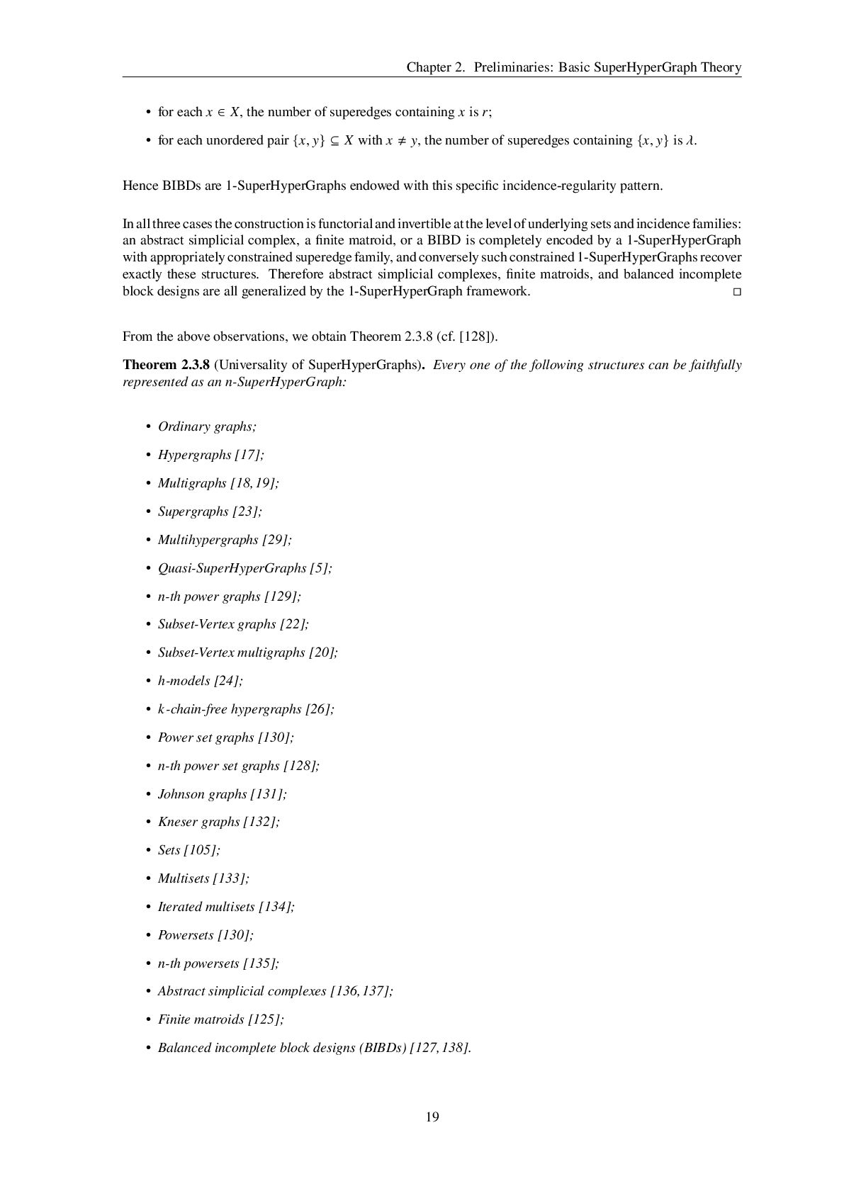
Chapter 2. Preliminaries: Basic SuperHyperGraph Theory • for each 𝑥
∈ 𝑋, the number of superedges containing 𝑥 is 𝑟; • for each unordered pair {𝑥, 𝑦} ⊆ 𝑋 with 𝑥 ≠ 𝑦, the number of superedges containing {𝑥, 𝑦} is 𝜆. Hence BIBDs are 1-SuperHyperGraphs endowed with this specific incidence-regularity pattern. In all three cases the construction is functorial and invertible at the level of underlying sets and incidence families: an abstract simplicial complex, a finite matroid, or a BIBD is completely encoded by a 1-SuperHyperGraph with appropriately constrained superedge family, and conversely such constrained 1-SuperHyperGraphs recover exactly these structures. Therefore abstract simplicial complexes, finite matroids, and balanced incomplete block designs are all generalized by the 1-SuperHyperGraph framework. □ From the above observations, we obtain Theorem 2.3.8 (cf. [128]). Theorem 2.3.8 (Universality of SuperHyperGraphs). Every one of the following structures can be faithfully represented as an 𝑛-SuperHyperGraph: • Ordinary graphs; • Hypergraphs [17]; • Multigraphs [18,19]; • Supergraphs [23]; • Multihypergraphs [29]; • Quasi-SuperHyperGraphs [5]; • 𝑛-th power graphs [129]; • Subset-Vertex graphs [22]; • Subset-Vertex multigraphs [20]; • ℎ-models [24]; • 𝑘-chain-free hypergraphs [26]; • Power set graphs [130]; • 𝑛-th power set graphs [128]; • Johnson graphs [131]; • Kneser graphs [132]; • Sets [105]; • Multisets [133]; • Iterated multisets [134]; • Powersets [130]; • 𝑛-th powersets [135]; • Abstract simplicial complexes [136,137]; • Finite matroids [125]; • Balanced incomplete block designs (BIBDs) [127,138]. 19

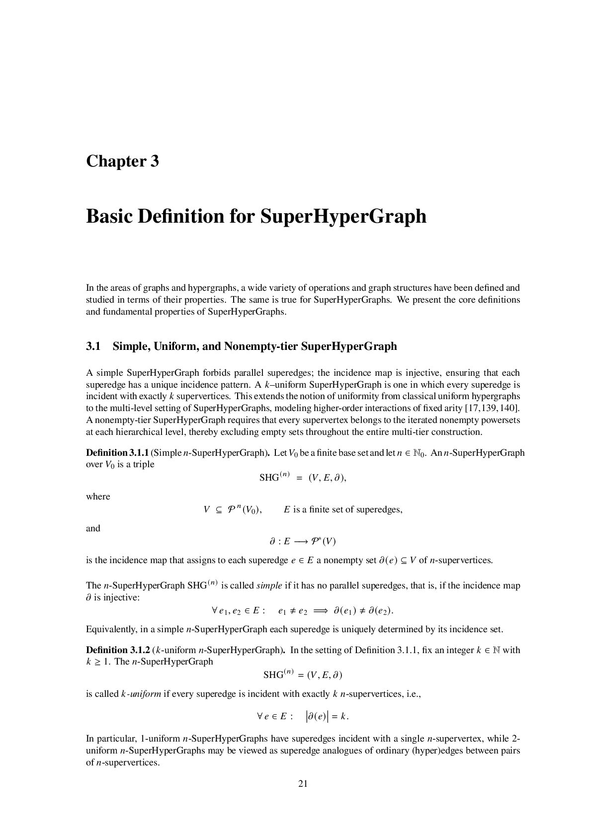
Chapter 2. Preliminaries: Basic SuperHyperGraph Theory 20

Chapter 3 Basic Definition for SuperHyperGraph In the areas of
graphs and hypergraphs, a wide variety of operations and graph structures have been defined and studied in terms of their properties. The same is true for SuperHyperGraphs. We present the core definitions and fundamental properties of SuperHyperGraphs. 3.1 Simple, Uniform, and Nonempty-tier SuperHyperGraph A simple SuperHyperGraph forbids parallel superedges; the incidence map is injective, ensuring that each superedge has a unique incidence pattern. A 𝑘–uniform SuperHyperGraph is one in which every superedge is incident with exactly 𝑘 supervertices. This extends the notion of uniformity from classical uniform hypergraphs to the multi-level setting of SuperHyperGraphs, modeling higher-order interactions of fixed arity [17,139,140]. A nonempty-tier SuperHyperGraph requires that every supervertex belongs to the iterated nonempty powersets at each hierarchical level, thereby excluding empty sets throughout the entire multi-tier construction. Definition 3.1.1(Simple 𝑛-SuperHyperGraph). Let𝑉0 beafinitebasesetandlet 𝑛 ∈ N0. An 𝑛-SuperHyperGraph over 𝑉0 is a triple SHG(𝑛) = (𝑉, 𝐸, 𝜕), where 𝑉 ⊆ P 𝑛(𝑉0 ), 𝐸 is a finite set of superedges, and 𝜕 : 𝐸 −→ P∗(𝑉) is the incidence map that assigns to each superedge 𝑒 ∈ 𝐸 a nonempty set 𝜕(𝑒) ⊆ 𝑉 of 𝑛-supervertices. The 𝑛-SuperHyperGraph SHG(𝑛) is called simple if it has no parallel superedges, that is, if the incidence map 𝜕 is injective: ∀ 𝑒1, 𝑒2 ∈ 𝐸 : 𝑒1 ≠ 𝑒2 =⇒ 𝜕(𝑒1 ) ≠ 𝜕(𝑒2 ). Equivalently, in a simple 𝑛-SuperHyperGraph each superedge is uniquely determined by its incidence set. Definition 3.1.2 (𝑘-uniform 𝑛-SuperHyperGraph). In the setting of Definition 3.1.1, fix an integer 𝑘 ∈ N with 𝑘 ≥ 1. The 𝑛-SuperHyperGraph SHG(𝑛) = (𝑉, 𝐸, 𝜕) is called 𝑘-uniform if every superedge is incident with exactly 𝑘 𝑛-supervertices, i.e., ∀ 𝑒 ∈ 𝐸 : 𝜕(𝑒) = 𝑘. In particular, 1-uniform 𝑛-SuperHyperGraphs have superedges incident with a single 𝑛-supervertex, while 2- uniform 𝑛-SuperHyperGraphs may be viewed as superedge analogues of ordinary (hyper)edges between pairs of 𝑛-supervertices. 21

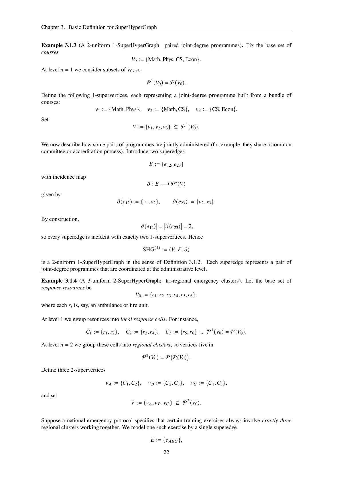
Chapter 3. Basic Definition for SuperHyperGraph Example 3.1.3 (A 2-uniform
1-SuperHyperGraph: paired joint-degree programmes). Fix the base set of courses 𝑉0 := {Math, Phys, CS, Econ}. At level 𝑛 = 1 we consider subsets of 𝑉0, so P1(𝑉0 ) = P(𝑉0 ). Define the following 1-supervertices, each representing a joint-degree programme built from a bundle of courses: 𝑣1 := {Math, Phys}, 𝑣2 := {Math, CS}, 𝑣3 := {CS, Econ}. Set 𝑉 := {𝑣1, 𝑣2, 𝑣3 } ⊆ P1(𝑉0 ). We now describe how some pairs of programmes are jointly administered (for example, they share a common committee or accreditation process). Introduce two superedges 𝐸 := {𝑒12, 𝑒23 } with incidence map 𝜕 : 𝐸 −→ P∗(𝑉) given by 𝜕(𝑒12 ) := {𝑣1, 𝑣2 }, 𝜕(𝑒23 ) := {𝑣2, 𝑣3 }. By construction, 𝜕(𝑒12 ) = 𝜕(𝑒23 ) = 2, so every superedge is incident with exactly two 1-supervertices. Hence SHG(1) := (𝑉, 𝐸, 𝜕) is a 2-uniform 1-SuperHyperGraph in the sense of Definition 3.1.2. Each superedge represents a pair of joint-degree programmes that are coordinated at the administrative level. Example 3.1.4 (A 3-uniform 2-SuperHyperGraph: tri-regional emergency clusters). Let the base set of response resources be 𝑉0 := {𝑟1, 𝑟2, 𝑟3, 𝑟4, 𝑟5, 𝑟6 }, where each 𝑟𝑖 is, say, an ambulance or fire unit. At level 1 we group resources into local response cells. For instance, 𝐶1 := {𝑟1, 𝑟2 }, 𝐶2 := {𝑟3, 𝑟4 }, 𝐶3 := {𝑟5, 𝑟6 } ∈ P1(𝑉0 ) = P(𝑉0 ). At level 𝑛 = 2 we group these cells into regional clusters, so vertices live in P2(𝑉0 ) = P P(𝑉0 ) . Define three 2-supervertices 𝑣𝐴 := {𝐶1, 𝐶2 }, 𝑣𝐵 := {𝐶2, 𝐶3 }, 𝑣𝐶 := {𝐶1, 𝐶3 }, and set 𝑉 := {𝑣𝐴, 𝑣𝐵, 𝑣𝐶 } ⊆ P2(𝑉0 ). Suppose a national emergency protocol specifies that certain training exercises always involve exactly three regional clusters working together. We model one such exercise by a single superedge 𝐸 := {𝑒𝐴𝐵𝐶 }, 22

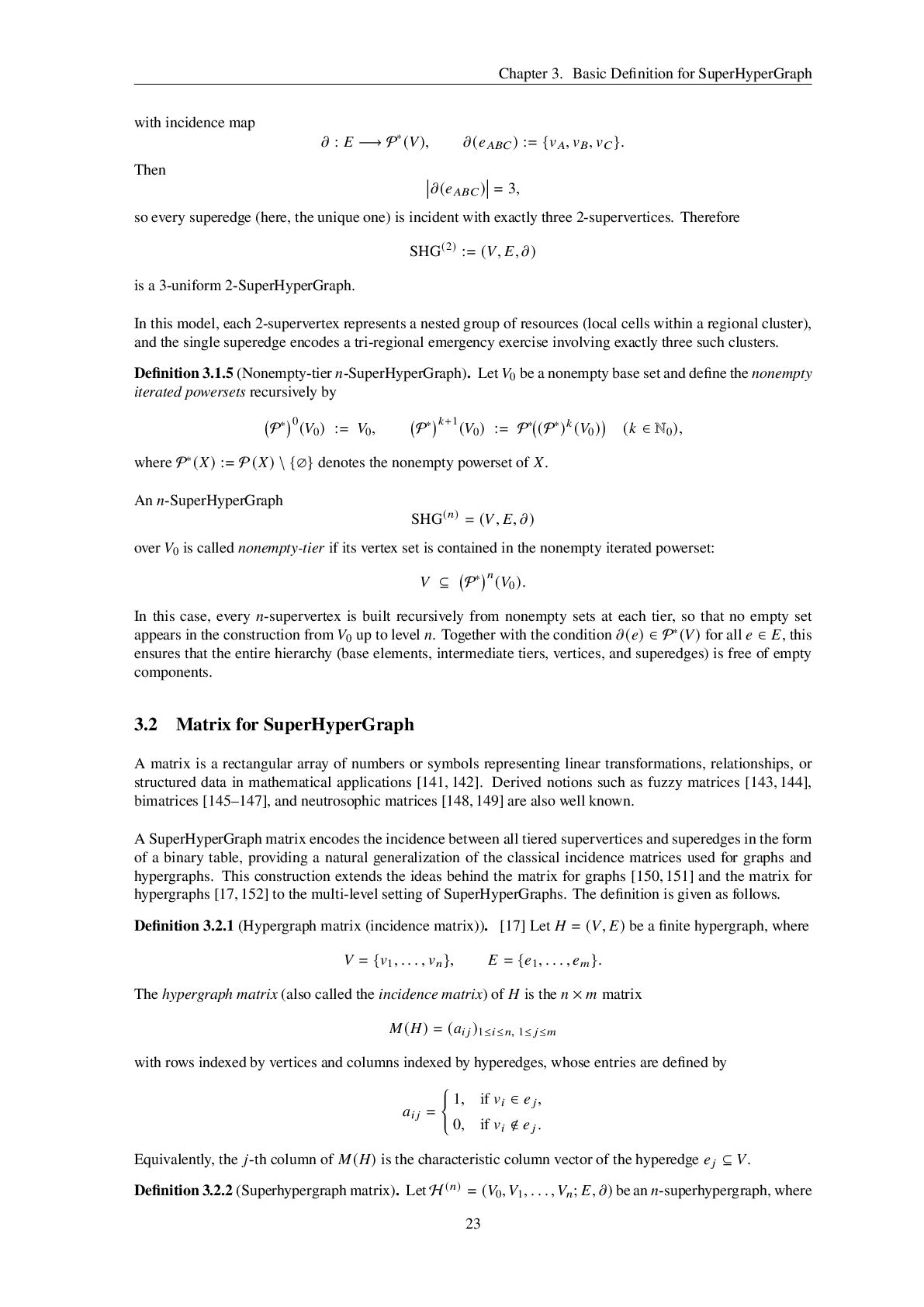
Chapter 3. Basic Definition for SuperHyperGraph with incidence map 𝜕
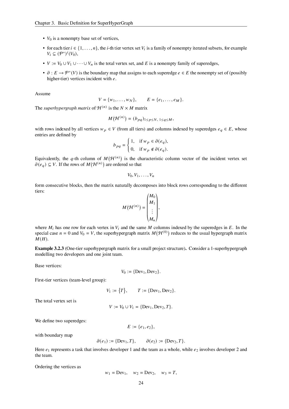
: 𝐸 −→ P∗(𝑉), 𝜕(𝑒𝐴𝐵𝐶 ) := {𝑣𝐴, 𝑣𝐵, 𝑣𝐶 }. Then 𝜕(𝑒𝐴𝐵𝐶 ) = 3, so every superedge (here, the unique one) is incident with exactly three 2-supervertices. Therefore SHG(2) := (𝑉, 𝐸, 𝜕) is a 3-uniform 2-SuperHyperGraph. In this model, each 2-supervertex represents a nested group of resources (local cells within a regional cluster), and the single superedge encodes a tri-regional emergency exercise involving exactly three such clusters. Definition 3.1.5 (Nonempty-tier 𝑛-SuperHyperGraph). Let 𝑉0 be a nonempty base set and define the nonempty iterated powersets recursively by P∗ 0(𝑉0 ) := 𝑉0, P∗ 𝑘+1(𝑉0 ) := P∗ (P∗)𝑘 (𝑉0 ) (𝑘 ∈ N0 ), where P∗(𝑋) := P(𝑋) \ {∅} denotes the nonempty powerset of 𝑋. An 𝑛-SuperHyperGraph SHG(𝑛) = (𝑉, 𝐸, 𝜕) over 𝑉0 is called nonempty-tier if its vertex set is contained in the nonempty iterated powerset: 𝑉 ⊆ P∗ 𝑛(𝑉0 ). In this case, every 𝑛-supervertex is built recursively from nonempty sets at each tier, so that no empty set appears in the construction from 𝑉0 up to level 𝑛. Together with the condition 𝜕(𝑒) ∈ P∗(𝑉) for all 𝑒 ∈ 𝐸, this ensures that the entire hierarchy (base elements, intermediate tiers, vertices, and superedges) is free of empty components. 3.2 Matrix for SuperHyperGraph A matrix is a rectangular array of numbers or symbols representing linear transformations, relationships, or structured data in mathematical applications [141, 142]. Derived notions such as fuzzy matrices [143, 144], bimatrices [145–147], and neutrosophic matrices [148,149] are also well known. A SuperHyperGraph matrix encodes the incidence between all tiered supervertices and superedges in the form of a binary table, providing a natural generalization of the classical incidence matrices used for graphs and hypergraphs. This construction extends the ideas behind the matrix for graphs [150, 151] and the matrix for hypergraphs [17,152] to the multi-level setting of SuperHyperGraphs. The definition is given as follows. Definition 3.2.1 (Hypergraph matrix (incidence matrix)). [17] Let 𝐻 = (𝑉, 𝐸) be a finite hypergraph, where 𝑉 = {𝑣1, . . . , 𝑣𝑛 }, 𝐸 = {𝑒1, . . . , 𝑒𝑚 }. The hypergraph matrix (also called the incidence matrix) of 𝐻 is the 𝑛 × 𝑚 matrix 𝑀(𝐻) = (𝑎𝑖 𝑗 )1≤𝑖≤𝑛, 1≤ 𝑗≤𝑚 with rows indexed by vertices and columns indexed by hyperedges, whose entries are defined by 𝑎𝑖 𝑗 = 1, if 𝑣𝑖 ∈ 𝑒𝑗, 0, if 𝑣𝑖 ∉ 𝑒𝑗 . Equivalently, the 𝑗-th column of 𝑀(𝐻) is the characteristic column vector of the hyperedge 𝑒𝑗 ⊆ 𝑉. Definition 3.2.2 (Superhypergraph matrix). Let H (𝑛) = (𝑉0,𝑉1, . . . ,𝑉𝑛 ; 𝐸, 𝜕) be an 𝑛-superhypergraph, where 23

Chapter 3. Basic Definition for SuperHyperGraph • 𝑉0 is a
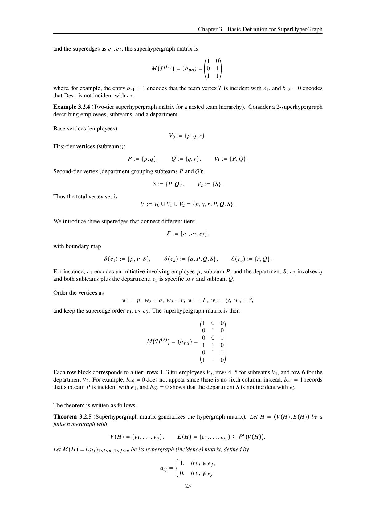
nonempty base set of vertices, • for each tier 𝑖 ∈ {1, . . . , 𝑛}, the 𝑖-th tier vertex set 𝑉𝑖 is a family of nonempty iterated subsets, for example 𝑉𝑖 ⊆ (P∗)𝑖 (𝑉0 ), • 𝑉 := 𝑉0 ∪ 𝑉1 ∪ · · · ∪ 𝑉𝑛 is the total vertex set, and 𝐸 is a nonempty family of superedges, • 𝜕 : 𝐸 → P∗(𝑉) is the boundary map that assigns to each superedge 𝑒 ∈ 𝐸 the nonempty set of (possibly higher-tier) vertices incident with 𝑒. Assume 𝑉 = {𝑤1, . . . , 𝑤𝑁 }, 𝐸 = {𝑒1, . . . , 𝑒𝑀 }. The superhypergraph matrix of H (𝑛) is the 𝑁 × 𝑀 matrix 𝑀 H (𝑛) = (𝑏𝑝𝑞 )1≤ 𝑝≤𝑁, 1≤𝑞≤𝑀, with rows indexed by all vertices 𝑤𝑝 ∈ 𝑉 (from all tiers) and columns indexed by superedges 𝑒𝑞 ∈ 𝐸, whose entries are defined by 𝑏𝑝𝑞 = 1, if 𝑤𝑝 ∈ 𝜕(𝑒𝑞 ), 0, if 𝑤𝑝 ∉ 𝜕(𝑒𝑞 ). Equivalently, the 𝑞-th column of 𝑀 H (𝑛) is the characteristic column vector of the incident vertex set 𝜕(𝑒𝑞 ) ⊆ 𝑉. If the rows of 𝑀 H (𝑛) are ordered so that 𝑉0,𝑉1, . . . ,𝑉𝑛 form consecutive blocks, then the matrix naturally decomposes into block rows corresponding to the different tiers: 𝑀 H (𝑛) = 𝑀0 𝑀1 . . . 𝑀𝑛 , where 𝑀𝑖 has one row for each vertex in 𝑉𝑖 and the same 𝑀 columns indexed by the superedges in 𝐸. In the special case 𝑛 = 0 and 𝑉0 = 𝑉, the superhypergraph matrix 𝑀 H (0) reduces to the usual hypergraph matrix 𝑀(𝐻). Example 3.2.3 (One-tier superhypergraph matrix for a small project structure). Consider a 1-superhypergraph modelling two developers and one joint team. Base vertices: 𝑉0 := {Dev1, Dev2 }. First-tier vertices (team-level group): 𝑉1 := 𝑇 , 𝑇 := {Dev1, Dev2 }. The total vertex set is 𝑉 := 𝑉0 ∪ 𝑉1 = {Dev1, Dev2,𝑇}. We define two superedges: 𝐸 := {𝑒1, 𝑒2 }, with boundary map 𝜕(𝑒1 ) := {Dev1,𝑇}, 𝜕(𝑒2 ) := {Dev2,𝑇}. Here 𝑒1 represents a task that involves developer 1 and the team as a whole, while 𝑒2 involves developer 2 and the team. Ordering the vertices as 𝑤1 = Dev1, 𝑤2 = Dev2, 𝑤3 = 𝑇, 24

Chapter 3. Basic Definition for SuperHyperGraph and the superedges as
𝑒1, 𝑒2, the superhypergraph matrix is 𝑀 H (1) = (𝑏𝑝𝑞 ) = 1 0 0 1 1 1 , where, for example, the entry 𝑏31 = 1 encodes that the team vertex 𝑇 is incident with 𝑒1, and 𝑏12 = 0 encodes that Dev1 is not incident with 𝑒2. Example 3.2.4 (Two-tier superhypergraph matrix for a nested team hierarchy). Consider a 2-superhypergraph describing employees, subteams, and a department. Base vertices (employees): 𝑉0 := {𝑝, 𝑞, 𝑟}. First-tier vertices (subteams): 𝑃 := {𝑝, 𝑞}, 𝑄 := {𝑞, 𝑟}, 𝑉1 := {𝑃, 𝑄}. Second-tier vertex (department grouping subteams 𝑃 and 𝑄): 𝑆 := {𝑃, 𝑄}, 𝑉2 := {𝑆}. Thus the total vertex set is 𝑉 := 𝑉0 ∪ 𝑉1 ∪ 𝑉2 = {𝑝, 𝑞, 𝑟, 𝑃, 𝑄, 𝑆}. We introduce three superedges that connect different tiers: 𝐸 := {𝑒1, 𝑒2, 𝑒3 }, with boundary map 𝜕(𝑒1 ) := {𝑝, 𝑃, 𝑆}, 𝜕(𝑒2 ) := {𝑞, 𝑃, 𝑄, 𝑆}, 𝜕(𝑒3 ) := {𝑟, 𝑄}. For instance, 𝑒1 encodes an initiative involving employee 𝑝, subteam 𝑃, and the department 𝑆; 𝑒2 involves 𝑞 and both subteams plus the department; 𝑒3 is specific to 𝑟 and subteam 𝑄. Order the vertices as 𝑤1 = 𝑝, 𝑤2 = 𝑞, 𝑤3 = 𝑟, 𝑤4 = 𝑃, 𝑤5 = 𝑄, 𝑤6 = 𝑆, and keep the superedge order 𝑒1, 𝑒2, 𝑒3. The superhypergraph matrix is then 𝑀 H (2) = (𝑏𝑝𝑞 ) = 1 0 0 0 1 0 0 0 1 1 1 0 0 1 1 1 1 0 . Each row block corresponds to a tier: rows 1–3 for employees 𝑉0, rows 4–5 for subteams 𝑉1, and row 6 for the department 𝑉2. For example, 𝑏46 = 0 does not appear since there is no sixth column; instead, 𝑏41 = 1 records that subteam 𝑃 is incident with 𝑒1, and 𝑏63 = 0 shows that the department 𝑆 is not incident with 𝑒3. The theorem is written as follows. Theorem 3.2.5 (Superhypergraph matrix generalizes the hypergraph matrix). Let 𝐻 = (𝑉(𝐻), 𝐸(𝐻)) be a finite hypergraph with 𝑉(𝐻) = {𝑣1, . . . , 𝑣𝑛 }, 𝐸(𝐻) = {𝑒1, . . . , 𝑒𝑚 } ⊆ P∗ 𝑉(𝐻) . Let 𝑀(𝐻) = (𝑎𝑖 𝑗 )1≤𝑖≤𝑛, 1≤ 𝑗≤𝑚 be its hypergraph (incidence) matrix, defined by 𝑎𝑖 𝑗 = 1, if 𝑣𝑖 ∈ 𝑒𝑗, 0, if 𝑣𝑖 ∉ 𝑒𝑗 . 25

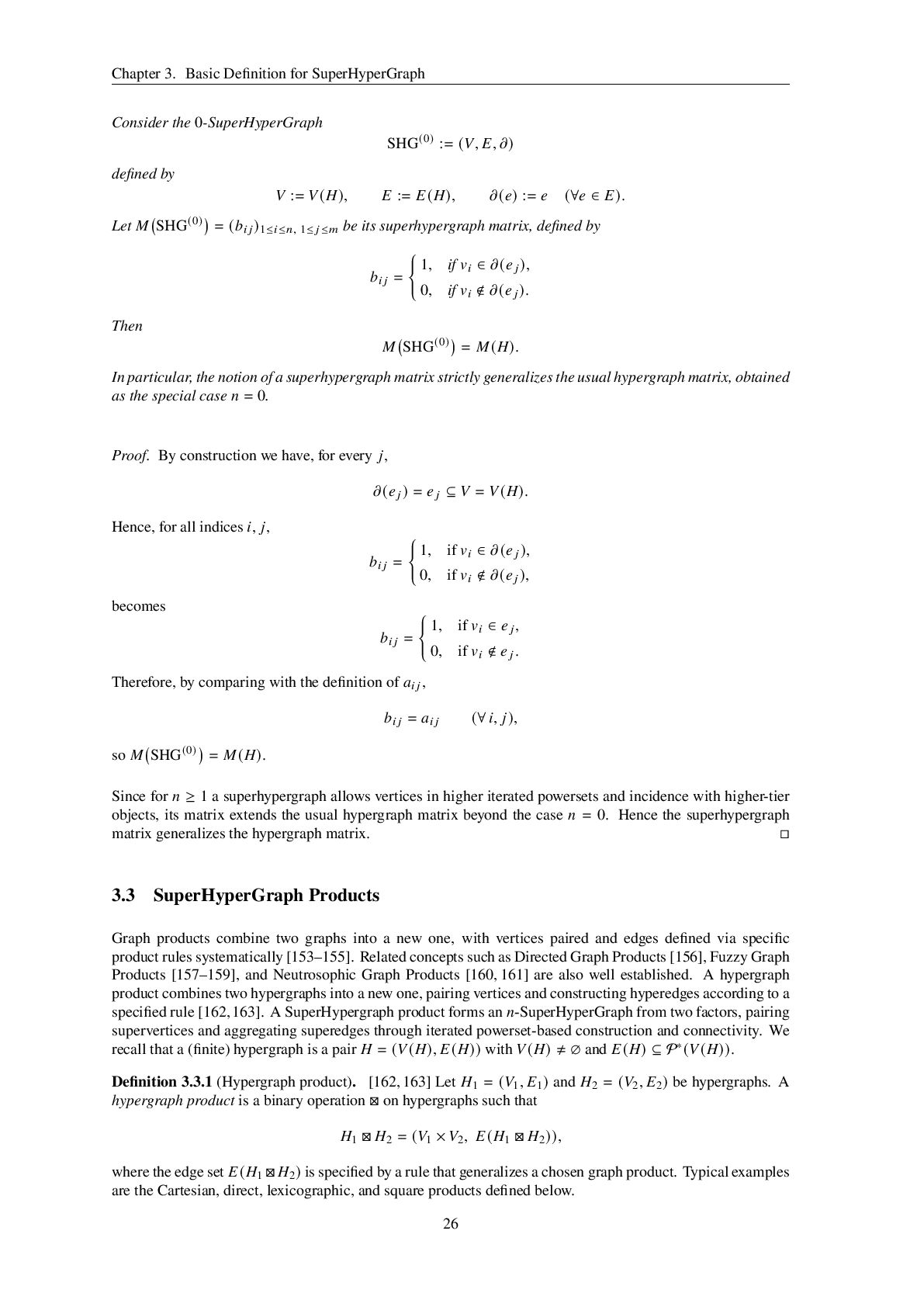
Chapter 3. Basic Definition for SuperHyperGraph Consider the 0-SuperHyperGraph SHG(0)
:= (𝑉, 𝐸, 𝜕) defined by 𝑉 := 𝑉(𝐻), 𝐸 := 𝐸(𝐻), 𝜕(𝑒) := 𝑒 (∀𝑒 ∈ 𝐸). Let 𝑀 SHG(0) = (𝑏𝑖 𝑗 )1≤𝑖≤𝑛, 1≤ 𝑗≤𝑚 be its superhypergraph matrix, defined by 𝑏𝑖 𝑗 = 1, if 𝑣𝑖 ∈ 𝜕(𝑒𝑗 ), 0, if 𝑣𝑖 ∉ 𝜕(𝑒𝑗 ). Then 𝑀 SHG(0) = 𝑀(𝐻). In particular, the notion of a superhypergraph matrix strictly generalizes the usual hypergraph matrix, obtained as the special case 𝑛 = 0. Proof. By construction we have, for every 𝑗, 𝜕(𝑒𝑗 ) = 𝑒𝑗 ⊆ 𝑉 = 𝑉(𝐻). Hence, for all indices 𝑖, 𝑗, 𝑏𝑖 𝑗 = 1, if 𝑣𝑖 ∈ 𝜕(𝑒𝑗 ), 0, if 𝑣𝑖 ∉ 𝜕(𝑒𝑗 ), becomes 𝑏𝑖 𝑗 = 1, if 𝑣𝑖 ∈ 𝑒𝑗, 0, if 𝑣𝑖 ∉ 𝑒𝑗 . Therefore, by comparing with the definition of 𝑎𝑖 𝑗 , 𝑏𝑖 𝑗 = 𝑎𝑖 𝑗 (∀𝑖, 𝑗), so 𝑀 SHG(0) = 𝑀(𝐻). Since for 𝑛 ≥ 1 a superhypergraph allows vertices in higher iterated powersets and incidence with higher-tier objects, its matrix extends the usual hypergraph matrix beyond the case 𝑛 = 0. Hence the superhypergraph matrix generalizes the hypergraph matrix. □ 3.3 SuperHyperGraph Products Graph products combine two graphs into a new one, with vertices paired and edges defined via specific product rules systematically [153–155]. Related concepts such as Directed Graph Products [156], Fuzzy Graph Products [157–159], and Neutrosophic Graph Products [160, 161] are also well established. A hypergraph product combines two hypergraphs into a new one, pairing vertices and constructing hyperedges according to a specified rule [162,163]. A SuperHypergraph product forms an 𝑛-SuperHyperGraph from two factors, pairing supervertices and aggregating superedges through iterated powerset-based construction and connectivity. We recall that a (finite) hypergraph is a pair 𝐻 = (𝑉(𝐻), 𝐸(𝐻)) with 𝑉(𝐻) ≠ ∅ and 𝐸(𝐻) ⊆ P∗(𝑉(𝐻)). Definition 3.3.1 (Hypergraph product). [162,163] Let 𝐻1 = (𝑉1, 𝐸1 ) and 𝐻2 = (𝑉2, 𝐸2 ) be hypergraphs. A hypergraph product is a binary operation ⊠ on hypergraphs such that 𝐻1 ⊠ 𝐻2 = (𝑉1 × 𝑉2, 𝐸(𝐻1 ⊠ 𝐻2 )), where the edge set 𝐸(𝐻1 ⊠ 𝐻2 ) is specified by a rule that generalizes a chosen graph product. Typical examples are the Cartesian, direct, lexicographic, and square products defined below. 26

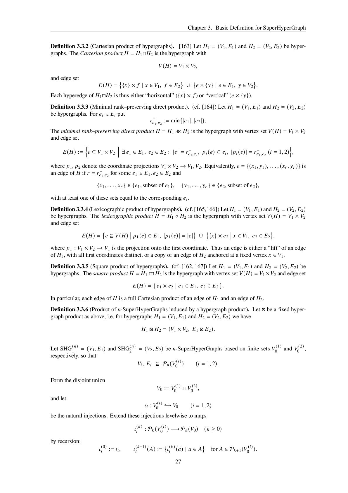
Chapter 3. Basic Definition for SuperHyperGraph Definition 3.3.2 (Cartesian product
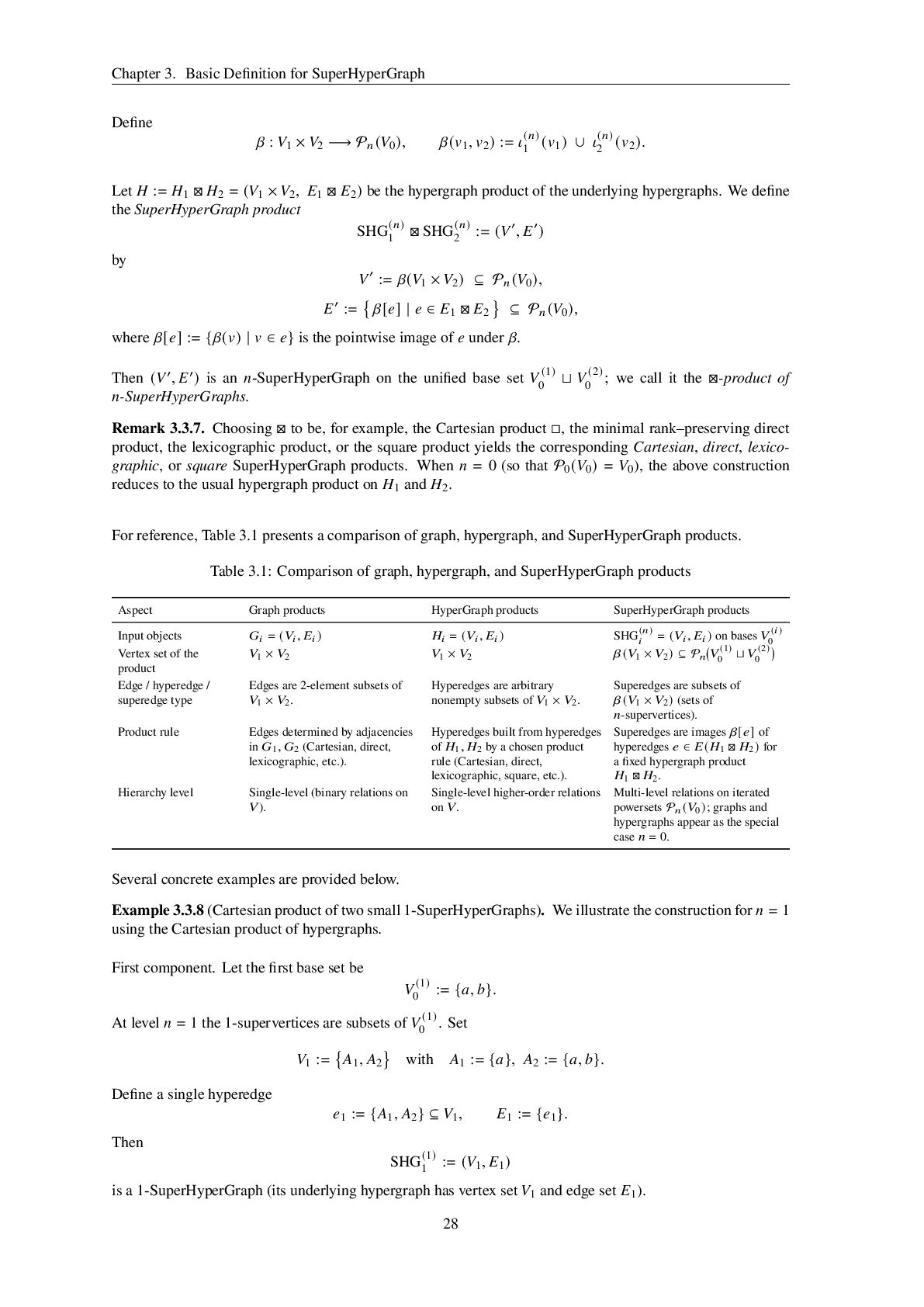
of hypergraphs). [163] Let 𝐻1 = (𝑉1, 𝐸1 ) and 𝐻2 = (𝑉2, 𝐸2 ) be hypergraphs. The Cartesian product 𝐻 = 𝐻1□𝐻2 is the hypergraph with 𝑉(𝐻) = 𝑉1 × 𝑉2, and edge set 𝐸(𝐻) = {𝑥} × 𝑓 | 𝑥 ∈ 𝑉1, 𝑓 ∈ 𝐸2 ∪ 𝑒 × {𝑦} | 𝑒 ∈ 𝐸1, 𝑦 ∈ 𝑉2 . Each hyperedge of 𝐻1□𝐻2 is thus either “horizontal” ({𝑥} × 𝑓 ) or “vertical” (𝑒 × {𝑦}). Definition 3.3.3 (Minimal rank–preserving direct product). (cf. [164]) Let 𝐻1 = (𝑉1, 𝐸1 ) and 𝐻2 = (𝑉2, 𝐸2 ) be hypergraphs. For 𝑒𝑖 ∈ 𝐸𝑖 put 𝑟− 𝑒1,𝑒2 := min{|𝑒1 |, |𝑒2 |}. The minimal rank–preserving direct product 𝐻 = 𝐻1 ⊩ × 𝐻2 is the hypergraph with vertex set 𝑉(𝐻) = 𝑉1 × 𝑉2 and edge set 𝐸(𝐻) := 𝑒 ⊆ 𝑉1 × 𝑉2 ∃ 𝑒1 ∈ 𝐸1, 𝑒2 ∈ 𝐸2 : |𝑒| = 𝑟− 𝑒1,𝑒2 , 𝑝𝑖 (𝑒) ⊆ 𝑒𝑖, |𝑝𝑖 (𝑒)| = 𝑟− 𝑒1,𝑒2 (𝑖 = 1, 2) , where 𝑝1, 𝑝2 denote the coordinate projections 𝑉1 × 𝑉2 → 𝑉1,𝑉2. Equivalently, 𝑒 = {(𝑥1, 𝑦1 ), . . . , (𝑥𝑟 , 𝑦𝑟 )} is an edge of 𝐻 if 𝑟 = 𝑟− 𝑒1,𝑒2 for some 𝑒1 ∈ 𝐸1, 𝑒2 ∈ 𝐸2 and {𝑥1, . . . , 𝑥𝑟 } ∈ {𝑒1, subset of 𝑒1 }, {𝑦1, . . . , 𝑦𝑟 } ∈ {𝑒2, subset of 𝑒2 }, with at least one of these sets equal to the corresponding 𝑒𝑖 . Definition 3.3.4 (Lexicographic product of hypergraphs). (cf. [165,166]) Let 𝐻1 = (𝑉1, 𝐸1 ) and 𝐻2 = (𝑉2, 𝐸2 ) be hypergraphs. The lexicographic product 𝐻 = 𝐻1 ◦ 𝐻2 is the hypergraph with vertex set 𝑉(𝐻) = 𝑉1 × 𝑉2 and edge set 𝐸(𝐻) = 𝑒 ⊆ 𝑉(𝐻) 𝑝1 (𝑒) ∈ 𝐸1, |𝑝1 (𝑒)| = |𝑒| ∪ {𝑥} × 𝑒2 𝑥 ∈ 𝑉1, 𝑒2 ∈ 𝐸2 , where 𝑝1 : 𝑉1 × 𝑉2 → 𝑉1 is the projection onto the first coordinate. Thus an edge is either a “lift” of an edge of 𝐻1, with all first coordinates distinct, or a copy of an edge of 𝐻2 anchored at a fixed vertex 𝑥 ∈ 𝑉1. Definition 3.3.5 (Square product of hypergraphs). (cf. [162, 167]) Let 𝐻1 = (𝑉1, 𝐸1 ) and 𝐻2 = (𝑉2, 𝐸2 ) be hypergraphs. The square product 𝐻 = 𝐻1 □ □ 𝐻2 is the hypergraph with vertex set 𝑉(𝐻) = 𝑉1 ×𝑉2 and edge set 𝐸(𝐻) = { 𝑒1 × 𝑒2 | 𝑒1 ∈ 𝐸1, 𝑒2 ∈ 𝐸2 }. In particular, each edge of 𝐻 is a full Cartesian product of an edge of 𝐻1 and an edge of 𝐻2. Definition 3.3.6 (Product of 𝑛-SuperHyperGraphs induced by a hypergraph product). Let ⊠ be a fixed hypergraph product as above, i.e. for hypergraphs 𝐻1 = (𝑉1, 𝐸1 ) and 𝐻2 = (𝑉2, 𝐸2 ) we have 𝐻1 ⊠ 𝐻2 = (𝑉1 × 𝑉2, 𝐸1 ⊠ 𝐸2 ). Let SHG(𝑛) 1 = (𝑉1, 𝐸1 ) and SHG(𝑛) 2 = (𝑉2, 𝐸2 ) be 𝑛-SuperHyperGraphs based on finite sets 𝑉 (1) 0 and 𝑉 (2) 0 , respectively, so that 𝑉𝑖, 𝐸𝑖 ⊆ P 𝑛 (𝑉 (𝑖) 0 ) (𝑖 = 1, 2). Form the disjoint union 𝑉0 := 𝑉 (1) 0 ⊔ 𝑉 (2) 0 , and let 𝜄𝑖 : 𝑉 (𝑖) 0 ↩→ 𝑉0 (𝑖 = 1, 2) be the natural injections. Extend these injections levelwise to maps 𝜄 (𝑘) 𝑖 : P 𝑘 (𝑉 (𝑖) 0 ) −→ P 𝑘 (𝑉0 ) (𝑘 ≥ 0) by recursion: 𝜄 (0) 𝑖 := 𝜄𝑖, 𝜄 (𝑘+1) 𝑖 (𝐴) := 𝜄 (𝑘) 𝑖 (𝑎) | 𝑎 ∈ 𝐴 for 𝐴 ∈ P 𝑘+1 (𝑉 (𝑖) 0 ). 27

Chapter 3. Basic Definition for SuperHyperGraph Define 𝛽 : 𝑉1
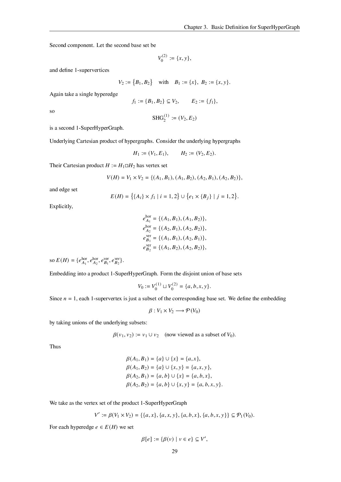
× 𝑉2 −→ P 𝑛 (𝑉0 ), 𝛽(𝑣1, 𝑣2 ) := 𝜄 (𝑛) 1 (𝑣1 ) ∪ 𝜄 (𝑛) 2 (𝑣2 ). Let 𝐻 := 𝐻1 ⊠ 𝐻2 = (𝑉1 × 𝑉2, 𝐸1 ⊠ 𝐸2 ) be the hypergraph product of the underlying hypergraphs. We define the SuperHyperGraph product SHG(𝑛) 1 ⊠ SHG(𝑛) 2 := (𝑉′ , 𝐸′) by 𝑉′ := 𝛽(𝑉1 × 𝑉2 ) ⊆ P 𝑛 (𝑉0 ), 𝐸′ := 𝛽[𝑒] | 𝑒 ∈ 𝐸1 ⊠ 𝐸2 ⊆ P 𝑛 (𝑉0 ), where 𝛽[𝑒] := {𝛽(𝑣) | 𝑣 ∈ 𝑒} is the pointwise image of 𝑒 under 𝛽. Then (𝑉′ , 𝐸′) is an 𝑛-SuperHyperGraph on the unified base set 𝑉 (1) 0 ⊔ 𝑉 (2) 0 ; we call it the ⊠-product of 𝑛-SuperHyperGraphs. Remark 3.3.7. Choosing ⊠ to be, for example, the Cartesian product □, the minimal rank–preserving direct product, the lexicographic product, or the square product yields the corresponding Cartesian, direct, lexicographic, or square SuperHyperGraph products. When 𝑛 = 0 (so that P0 (𝑉0 ) = 𝑉0), the above construction reduces to the usual hypergraph product on 𝐻1 and 𝐻2. For reference, Table 3.1 presents a comparison of graph, hypergraph, and SuperHyperGraph products. Table 3.1: Comparison of graph, hypergraph, and SuperHyperGraph products Aspect Graph products HyperGraph products SuperHyperGraph products Input objects 𝐺𝑖 = (𝑉𝑖 , 𝐸𝑖 ) 𝐻𝑖 = (𝑉𝑖 , 𝐸𝑖 ) SHG(𝑛) 𝑖 = (𝑉𝑖 , 𝐸𝑖 ) on bases 𝑉 (𝑖) 0 Vertex set of the product 𝑉1 × 𝑉2 𝑉1 × 𝑉2 𝛽(𝑉1 × 𝑉2) ⊆ P 𝑛 𝑉 (1) 0 ⊔ 𝑉 (2) 0 Edge / hyperedge / superedge type Edges are 2-element subsets of 𝑉1 × 𝑉2. Hyperedges are arbitrary nonempty subsets of 𝑉1 × 𝑉2. Superedges are subsets of 𝛽(𝑉1 × 𝑉2) (sets of 𝑛-supervertices). Product rule Edges determined by adjacencies in 𝐺1, 𝐺2 (Cartesian, direct, lexicographic, etc.). Hyperedges built from hyperedges of 𝐻1, 𝐻2 by a chosen product rule (Cartesian, direct, lexicographic, square, etc.). Superedges are images 𝛽[𝑒] of hyperedges 𝑒 ∈ 𝐸(𝐻1 ⊠ 𝐻2) for a fixed hypergraph product 𝐻1 ⊠ 𝐻2. Hierarchy level Single-level (binary relations on 𝑉). Single-level higher-order relations on 𝑉. Multi-level relations on iterated powersets P 𝑛 (𝑉0); graphs and hypergraphs appear as the special case 𝑛 = 0. Several concrete examples are provided below. Example 3.3.8 (Cartesian product of two small 1-SuperHyperGraphs). We illustrate the construction for 𝑛 = 1 using the Cartesian product of hypergraphs. First component. Let the first base set be 𝑉 (1) 0 := {𝑎, 𝑏}. At level 𝑛 = 1 the 1-supervertices are subsets of 𝑉 (1) 0 . Set 𝑉1 := 𝐴1, 𝐴2 with 𝐴1 := {𝑎}, 𝐴2 := {𝑎, 𝑏}. Define a single hyperedge 𝑒1 := {𝐴1, 𝐴2 } ⊆ 𝑉1, 𝐸1 := {𝑒1 }. Then SHG(1) 1 := (𝑉1, 𝐸1 ) is a 1-SuperHyperGraph (its underlying hypergraph has vertex set 𝑉1 and edge set 𝐸1). 28

Chapter 3. Basic Definition for SuperHyperGraph Second component. Let the
second base set be 𝑉 (2) 0 := {𝑥, 𝑦}, and define 1-supervertices 𝑉2 := 𝐵1, 𝐵2 with 𝐵1 := {𝑥}, 𝐵2 := {𝑥, 𝑦}. Again take a single hyperedge 𝑓1 := {𝐵1, 𝐵2 } ⊆ 𝑉2, 𝐸2 := { 𝑓1 }, so SHG(1) 2 := (𝑉2, 𝐸2 ) is a second 1-SuperHyperGraph. Underlying Cartesian product of hypergraphs. Consider the underlying hypergraphs 𝐻1 := (𝑉1, 𝐸1 ), 𝐻2 := (𝑉2, 𝐸2 ). Their Cartesian product 𝐻 := 𝐻1□𝐻2 has vertex set 𝑉(𝐻) = 𝑉1 × 𝑉2 = {(𝐴1, 𝐵1 ), (𝐴1, 𝐵2 ), (𝐴2, 𝐵1 ), (𝐴2, 𝐵2 )}, and edge set 𝐸(𝐻) = {𝐴𝑖 } × 𝑓1 | 𝑖 = 1, 2 ∪ 𝑒1 × {𝐵𝑗 } | 𝑗 = 1, 2 . Explicitly, 𝑒hor 𝐴1 = {(𝐴1, 𝐵1 ), (𝐴1, 𝐵2 )}, 𝑒hor 𝐴2 = {(𝐴2, 𝐵1 ), (𝐴2, 𝐵2 )}, 𝑒ver 𝐵1 = {(𝐴1, 𝐵1 ), (𝐴2, 𝐵1 )}, 𝑒ver 𝐵2 = {(𝐴1, 𝐵2 ), (𝐴2, 𝐵2 )}, so 𝐸(𝐻) = {𝑒hor 𝐴1 , 𝑒hor 𝐴2 , 𝑒ver 𝐵1 , 𝑒ver 𝐵2 }. Embedding into a product 1-SuperHyperGraph. Form the disjoint union of base sets 𝑉0 := 𝑉 (1) 0 ⊔ 𝑉 (2) 0 = {𝑎, 𝑏, 𝑥, 𝑦}. Since 𝑛 = 1, each 1-supervertex is just a subset of the corresponding base set. We define the embedding 𝛽 : 𝑉1 × 𝑉2 −→ P(𝑉0 ) by taking unions of the underlying subsets: 𝛽(𝑣1, 𝑣2 ) := 𝑣1 ∪ 𝑣2 (now viewed as a subset of 𝑉0). Thus 𝛽(𝐴1, 𝐵1 ) = {𝑎} ∪ {𝑥} = {𝑎, 𝑥}, 𝛽(𝐴1, 𝐵2 ) = {𝑎} ∪ {𝑥, 𝑦} = {𝑎, 𝑥, 𝑦}, 𝛽(𝐴2, 𝐵1 ) = {𝑎, 𝑏} ∪ {𝑥} = {𝑎, 𝑏, 𝑥}, 𝛽(𝐴2, 𝐵2 ) = {𝑎, 𝑏} ∪ {𝑥, 𝑦} = {𝑎, 𝑏, 𝑥, 𝑦}. We take as the vertex set of the product 1-SuperHyperGraph 𝑉′ := 𝛽(𝑉1 × 𝑉2 ) = {{𝑎, 𝑥}, {𝑎, 𝑥, 𝑦}, {𝑎, 𝑏, 𝑥}, {𝑎, 𝑏, 𝑥, 𝑦}} ⊆ P1 (𝑉0 ). For each hyperedge 𝑒 ∈ 𝐸(𝐻) we set 𝛽[𝑒] := {𝛽(𝑣) | 𝑣 ∈ 𝑒} ⊆ 𝑉′ , 29

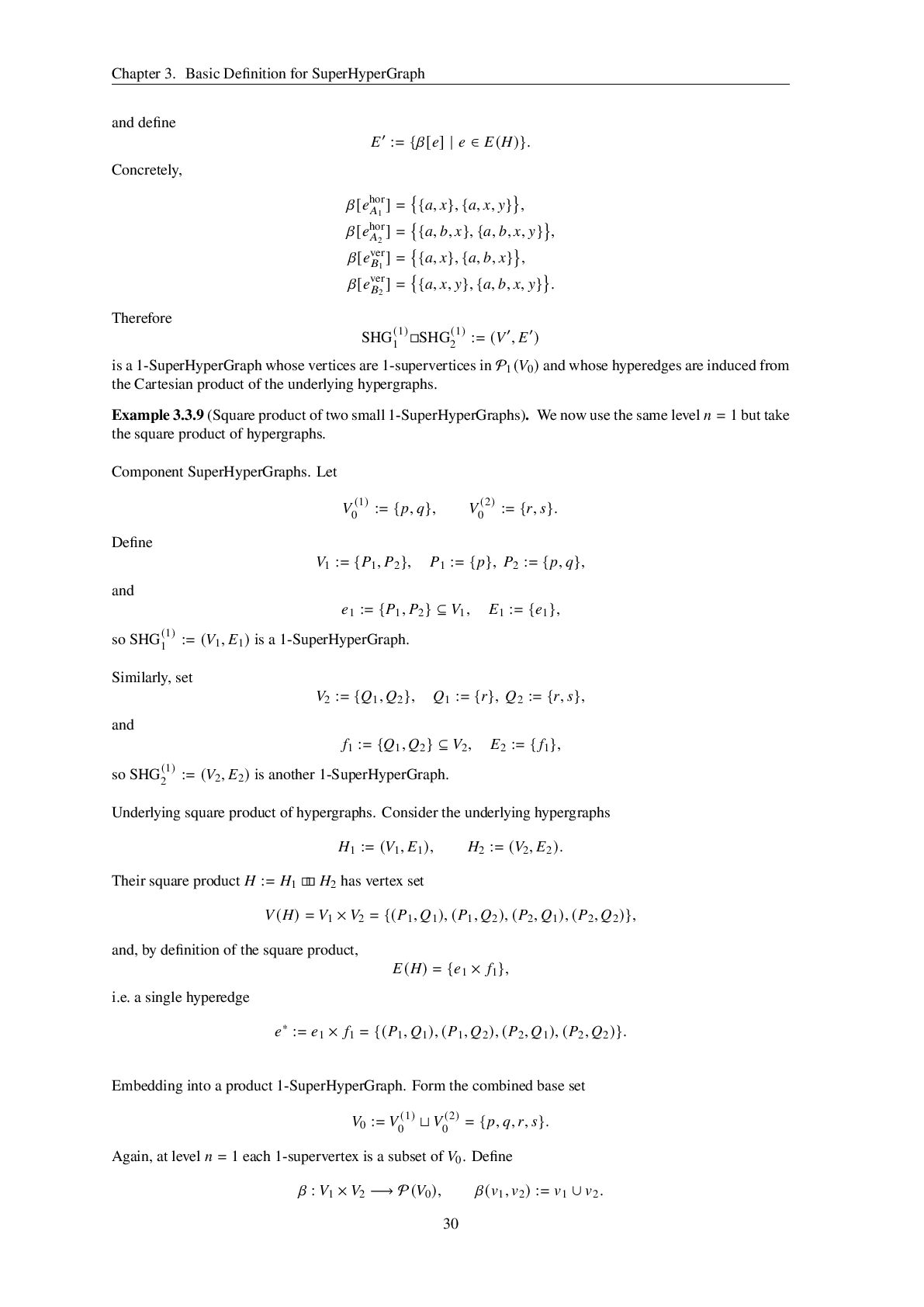
Chapter 3. Basic Definition for SuperHyperGraph and define 𝐸′ :=
{𝛽[𝑒] | 𝑒 ∈ 𝐸(𝐻)}. Concretely, 𝛽[𝑒hor 𝐴1 ] = {𝑎, 𝑥}, {𝑎, 𝑥, 𝑦} , 𝛽[𝑒hor 𝐴2 ] = {𝑎, 𝑏, 𝑥}, {𝑎, 𝑏, 𝑥, 𝑦} , 𝛽[𝑒ver 𝐵1 ] = {𝑎, 𝑥}, {𝑎, 𝑏, 𝑥} , 𝛽[𝑒ver 𝐵2 ] = {𝑎, 𝑥, 𝑦}, {𝑎, 𝑏, 𝑥, 𝑦} . Therefore SHG(1) 1 □SHG(1) 2 := (𝑉′ , 𝐸′) is a 1-SuperHyperGraph whose vertices are 1-supervertices in P1 (𝑉0 ) and whose hyperedges are induced from the Cartesian product of the underlying hypergraphs. Example 3.3.9 (Square product of two small 1-SuperHyperGraphs). We now use the same level 𝑛 = 1 but take the square product of hypergraphs. Component SuperHyperGraphs. Let 𝑉 (1) 0 := {𝑝, 𝑞}, 𝑉 (2) 0 := {𝑟, 𝑠}. Define 𝑉1 := {𝑃1, 𝑃2 }, 𝑃1 := {𝑝}, 𝑃2 := {𝑝, 𝑞}, and 𝑒1 := {𝑃1, 𝑃2 } ⊆ 𝑉1, 𝐸1 := {𝑒1 }, so SHG(1) 1 := (𝑉1, 𝐸1 ) is a 1-SuperHyperGraph. Similarly, set 𝑉2 := {𝑄1, 𝑄2 }, 𝑄1 := {𝑟}, 𝑄2 := {𝑟, 𝑠}, and 𝑓1 := {𝑄1, 𝑄2 } ⊆ 𝑉2, 𝐸2 := { 𝑓1 }, so SHG(1) 2 := (𝑉2, 𝐸2 ) is another 1-SuperHyperGraph. Underlying square product of hypergraphs. Consider the underlying hypergraphs 𝐻1 := (𝑉1, 𝐸1 ), 𝐻2 := (𝑉2, 𝐸2 ). Their square product 𝐻 := 𝐻1 □ □ 𝐻2 has vertex set 𝑉(𝐻) = 𝑉1 × 𝑉2 = {(𝑃1, 𝑄1 ), (𝑃1, 𝑄2 ), (𝑃2, 𝑄1 ), (𝑃2, 𝑄2 )}, and, by definition of the square product, 𝐸(𝐻) = {𝑒1 × 𝑓1 }, i.e. a single hyperedge 𝑒∗ := 𝑒1 × 𝑓1 = {(𝑃1, 𝑄1 ), (𝑃1, 𝑄2 ), (𝑃2, 𝑄1 ), (𝑃2, 𝑄2 )}. Embedding into a product 1-SuperHyperGraph. Form the combined base set 𝑉0 := 𝑉 (1) 0 ⊔ 𝑉 (2) 0 = {𝑝, 𝑞, 𝑟, 𝑠}. Again, at level 𝑛 = 1 each 1-supervertex is a subset of 𝑉0. Define 𝛽 : 𝑉1 × 𝑉2 −→ P(𝑉0 ), 𝛽(𝑣1, 𝑣2 ) := 𝑣1 ∪ 𝑣2. 30

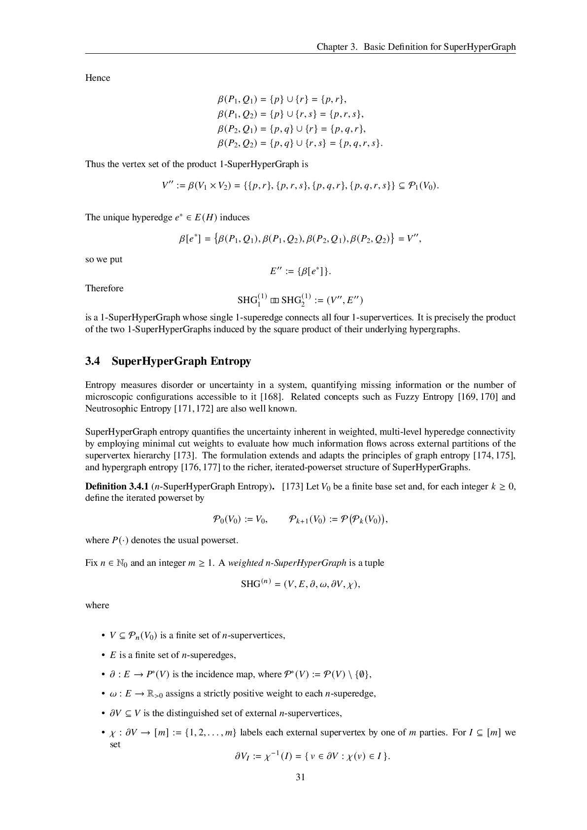
Chapter 3. Basic Definition for SuperHyperGraph Hence 𝛽(𝑃1, 𝑄1 )
= {𝑝} ∪ {𝑟} = {𝑝, 𝑟}, 𝛽(𝑃1, 𝑄2 ) = {𝑝} ∪ {𝑟, 𝑠} = {𝑝, 𝑟, 𝑠}, 𝛽(𝑃2, 𝑄1 ) = {𝑝, 𝑞} ∪ {𝑟} = {𝑝, 𝑞, 𝑟}, 𝛽(𝑃2, 𝑄2 ) = {𝑝, 𝑞} ∪ {𝑟, 𝑠} = {𝑝, 𝑞, 𝑟, 𝑠}. Thus the vertex set of the product 1-SuperHyperGraph is 𝑉′′ := 𝛽(𝑉1 × 𝑉2 ) = {{𝑝, 𝑟}, {𝑝, 𝑟, 𝑠}, {𝑝, 𝑞, 𝑟}, {𝑝, 𝑞, 𝑟, 𝑠}} ⊆ P1 (𝑉0 ). The unique hyperedge 𝑒∗ ∈ 𝐸(𝐻) induces 𝛽[𝑒∗] = 𝛽(𝑃1, 𝑄1 ), 𝛽(𝑃1, 𝑄2 ), 𝛽(𝑃2, 𝑄1 ), 𝛽(𝑃2, 𝑄2 ) = 𝑉′′ , so we put 𝐸′′ := {𝛽[𝑒∗]}. Therefore SHG(1) 1 □ □ SHG(1) 2 := (𝑉′′ , 𝐸′′) is a 1-SuperHyperGraph whose single 1-superedge connects all four 1-supervertices. It is precisely the product of the two 1-SuperHyperGraphs induced by the square product of their underlying hypergraphs. 3.4 SuperHyperGraph Entropy Entropy measures disorder or uncertainty in a system, quantifying missing information or the number of microscopic configurations accessible to it [168]. Related concepts such as Fuzzy Entropy [169, 170] and Neutrosophic Entropy [171,172] are also well known. SuperHyperGraph entropy quantifies the uncertainty inherent in weighted, multi-level hyperedge connectivity by employing minimal cut weights to evaluate how much information flows across external partitions of the supervertex hierarchy [173]. The formulation extends and adapts the principles of graph entropy [174, 175], and hypergraph entropy [176,177] to the richer, iterated-powerset structure of SuperHyperGraphs. Definition 3.4.1 (𝑛-SuperHyperGraph Entropy). [173] Let 𝑉0 be a finite base set and, for each integer 𝑘 ≥ 0, define the iterated powerset by P0 (𝑉0 ) := 𝑉0, P 𝑘+1 (𝑉0 ) := P P 𝑘 (𝑉0 ) , where 𝑃(·) denotes the usual powerset. Fix 𝑛 ∈ N0 and an integer 𝑚 ≥ 1. A weighted 𝑛-SuperHyperGraph is a tuple SHG(𝑛) = (𝑉, 𝐸, 𝜕, 𝜔, 𝜕𝑉, 𝜒), where • 𝑉 ⊆ P 𝑛 (𝑉0 ) is a finite set of 𝑛-supervertices, • 𝐸 is a finite set of 𝑛-superedges, • 𝜕 : 𝐸 → 𝑃∗(𝑉) is the incidence map, where P∗(𝑉) := P(𝑉) \ {∅}, • 𝜔 : 𝐸 → R>0 assigns a strictly positive weight to each 𝑛-superedge, • 𝜕𝑉 ⊆ 𝑉 is the distinguished set of external 𝑛-supervertices, • 𝜒 : 𝜕𝑉 → [𝑚] := {1, 2, . . . , 𝑚} labels each external supervertex by one of 𝑚 parties. For 𝐼 ⊆ [𝑚] we set 𝜕𝑉𝐼 := 𝜒−1(𝐼) = { 𝑣 ∈ 𝜕𝑉 : 𝜒(𝑣) ∈ 𝐼 }. 31

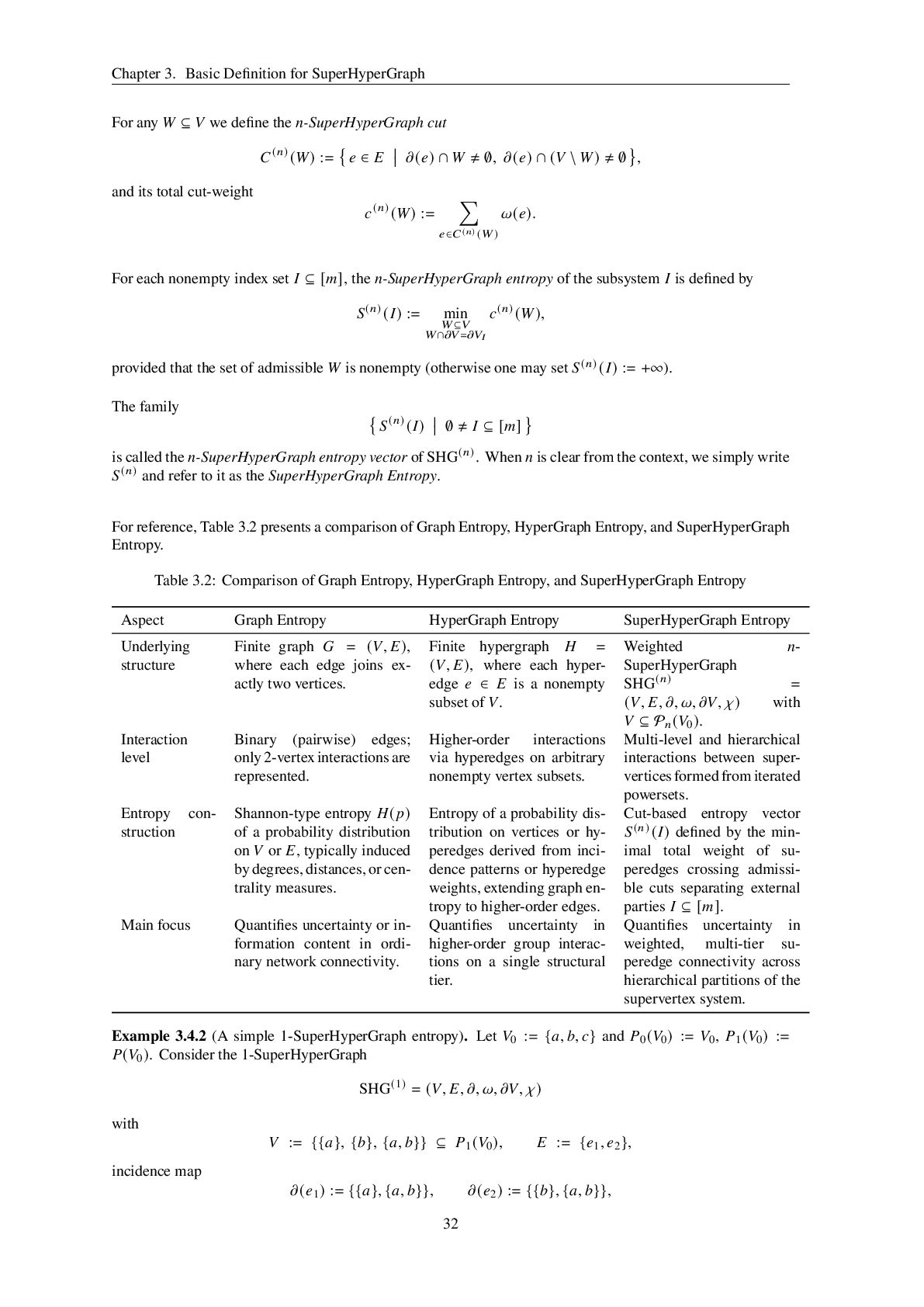
Chapter 3. Basic Definition for SuperHyperGraph For any 𝑊 ⊆
𝑉 we define the 𝑛-SuperHyperGraph cut 𝐶(𝑛) (𝑊) := 𝑒 ∈ 𝐸 𝜕(𝑒) ∩ 𝑊 ≠ ∅, 𝜕(𝑒) ∩ (𝑉 \ 𝑊) ≠ ∅ , and its total cut-weight 𝑐(𝑛) (𝑊) := ∑︁ 𝑒∈𝐶(𝑛) (𝑊) 𝜔(𝑒). For each nonempty index set 𝐼 ⊆ [𝑚], the 𝑛-SuperHyperGraph entropy of the subsystem 𝐼 is defined by 𝑆(𝑛) (𝐼) := min 𝑊⊆𝑉 𝑊∩𝜕𝑉=𝜕𝑉𝐼 𝑐(𝑛) (𝑊), provided that the set of admissible 𝑊 is nonempty (otherwise one may set 𝑆(𝑛) (𝐼) := +∞). The family 𝑆(𝑛) (𝐼) ∅ ≠ 𝐼 ⊆ [𝑚] is called the 𝑛-SuperHyperGraph entropy vector of SHG(𝑛). When 𝑛 is clear from the context, we simply write 𝑆(𝑛) and refer to it as the SuperHyperGraph Entropy. For reference, Table 3.2 presents a comparison of Graph Entropy, HyperGraph Entropy, and SuperHyperGraph Entropy. Table 3.2: Comparison of Graph Entropy, HyperGraph Entropy, and SuperHyperGraph Entropy Aspect Graph Entropy HyperGraph Entropy SuperHyperGraph Entropy Underlying structure Finite graph 𝐺 = (𝑉, 𝐸), where each edge joins exactly two vertices. Finite hypergraph 𝐻 = (𝑉, 𝐸), where each hyperedge 𝑒 ∈ 𝐸 is a nonempty subset of 𝑉. Weighted 𝑛- SuperHyperGraph SHG(𝑛) = (𝑉, 𝐸, 𝜕, 𝜔, 𝜕𝑉, 𝜒) with 𝑉 ⊆ P 𝑛 (𝑉0 ). Interaction level Binary (pairwise) edges; only 2-vertex interactions are represented. Higher-order interactions via hyperedges on arbitrary nonempty vertex subsets. Multi-level and hierarchical interactions between supervertices formed from iterated powersets. Entropy construction Shannon-type entropy 𝐻(𝑝) of a probability distribution on 𝑉 or 𝐸, typically induced by degrees, distances, or centrality measures. Entropy of a probability distribution on vertices or hyperedges derived from incidence patterns or hyperedge weights, extending graph entropy to higher-order edges. Cut-based entropy vector 𝑆(𝑛) (𝐼) defined by the minimal total weight of superedges crossing admissible cuts separating external parties 𝐼 ⊆ [𝑚]. Main focus Quantifies uncertainty or information content in ordinary network connectivity. Quantifies uncertainty in higher-order group interactions on a single structural tier. Quantifies uncertainty in weighted, multi-tier superedge connectivity across hierarchical partitions of the supervertex system. Example 3.4.2 (A simple 1-SuperHyperGraph entropy). Let 𝑉0 := {𝑎, 𝑏, 𝑐} and 𝑃0 (𝑉0 ) := 𝑉0, 𝑃1 (𝑉0 ) := 𝑃(𝑉0 ). Consider the 1-SuperHyperGraph SHG(1) = (𝑉, 𝐸, 𝜕, 𝜔, 𝜕𝑉, 𝜒) with 𝑉 := {{𝑎}, {𝑏}, {𝑎, 𝑏}} ⊆ 𝑃1 (𝑉0 ), 𝐸 := {𝑒1, 𝑒2 }, incidence map 𝜕(𝑒1 ) := {{𝑎}, {𝑎, 𝑏}}, 𝜕(𝑒2 ) := {{𝑏}, {𝑎, 𝑏}}, 32

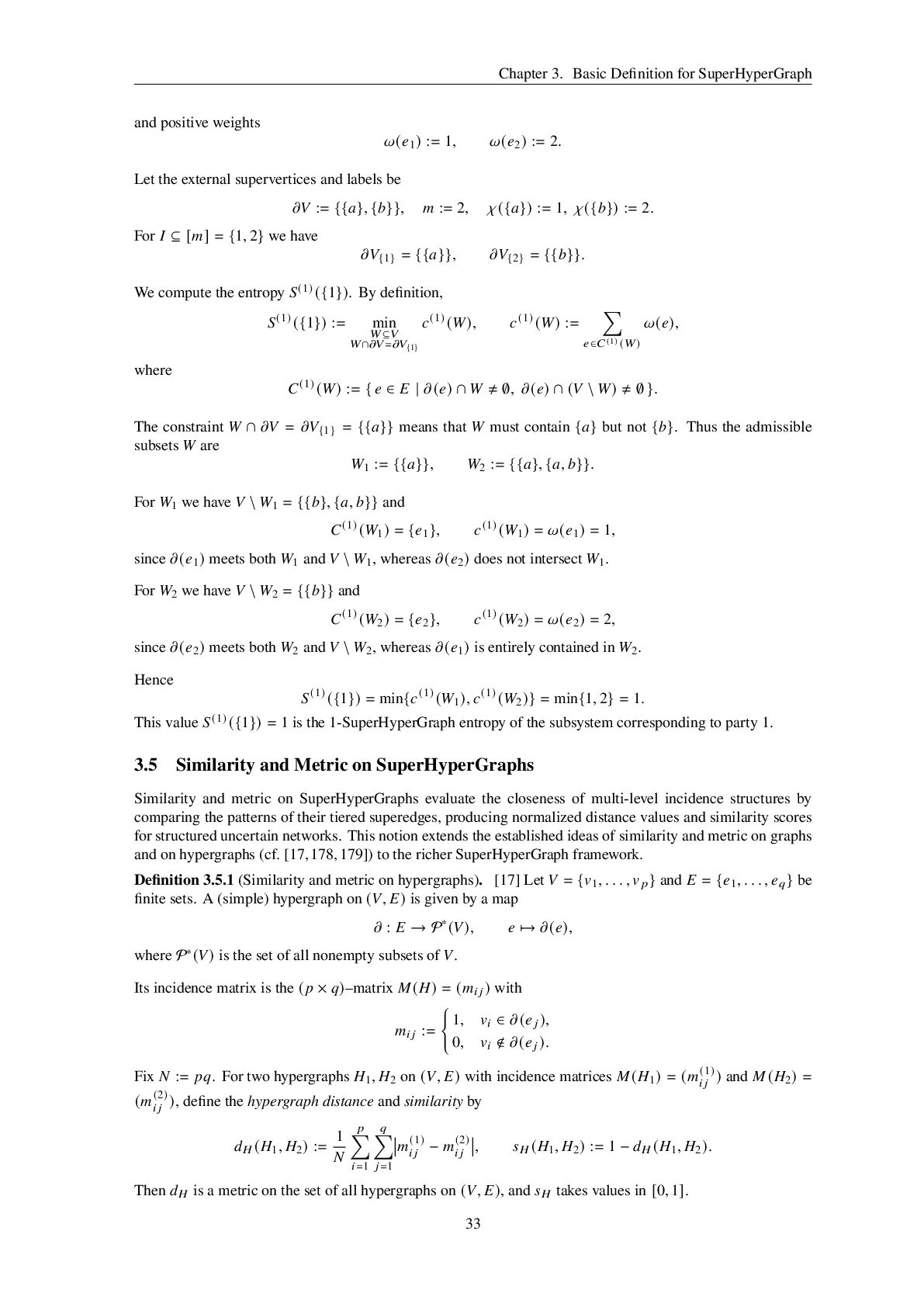
Chapter 3. Basic Definition for SuperHyperGraph and positive weights 𝜔(𝑒1
) := 1, 𝜔(𝑒2 ) := 2. Let the external supervertices and labels be 𝜕𝑉 := {{𝑎}, {𝑏}}, 𝑚 := 2, 𝜒({𝑎}) := 1, 𝜒({𝑏}) := 2. For 𝐼 ⊆ [𝑚] = {1, 2} we have 𝜕𝑉{1} = {{𝑎}}, 𝜕𝑉{2} = {{𝑏}}. We compute the entropy 𝑆(1) ({1}). By definition, 𝑆(1) ({1}) := min 𝑊⊆𝑉 𝑊∩𝜕𝑉=𝜕𝑉{1} 𝑐(1) (𝑊), 𝑐(1) (𝑊) := ∑︁ 𝑒∈𝐶(1) (𝑊) 𝜔(𝑒), where 𝐶(1) (𝑊) := { 𝑒 ∈ 𝐸 | 𝜕(𝑒) ∩ 𝑊 ≠ ∅, 𝜕(𝑒) ∩ (𝑉 \ 𝑊) ≠ ∅ }. The constraint 𝑊 ∩ 𝜕𝑉 = 𝜕𝑉{1} = {{𝑎}} means that 𝑊 must contain {𝑎} but not {𝑏}. Thus the admissible subsets 𝑊 are 𝑊1 := {{𝑎}}, 𝑊2 := {{𝑎}, {𝑎, 𝑏}}. For 𝑊1 we have 𝑉 \ 𝑊1 = {{𝑏}, {𝑎, 𝑏}} and 𝐶(1) (𝑊1 ) = {𝑒1 }, 𝑐(1) (𝑊1 ) = 𝜔(𝑒1 ) = 1, since 𝜕(𝑒1 ) meets both 𝑊1 and 𝑉 \ 𝑊1, whereas 𝜕(𝑒2 ) does not intersect 𝑊1. For 𝑊2 we have 𝑉 \ 𝑊2 = {{𝑏}} and 𝐶(1) (𝑊2 ) = {𝑒2 }, 𝑐(1) (𝑊2 ) = 𝜔(𝑒2 ) = 2, since 𝜕(𝑒2 ) meets both 𝑊2 and 𝑉 \ 𝑊2, whereas 𝜕(𝑒1 ) is entirely contained in 𝑊2. Hence 𝑆(1) ({1}) = min{𝑐(1) (𝑊1 ), 𝑐(1) (𝑊2 )} = min{1, 2} = 1. This value 𝑆(1) ({1}) = 1 is the 1-SuperHyperGraph entropy of the subsystem corresponding to party 1. 3.5 Similarity and Metric on SuperHyperGraphs Similarity and metric on SuperHyperGraphs evaluate the closeness of multi-level incidence structures by comparing the patterns of their tiered superedges, producing normalized distance values and similarity scores for structured uncertain networks. This notion extends the established ideas of similarity and metric on graphs and on hypergraphs (cf. [17,178,179]) to the richer SuperHyperGraph framework. Definition 3.5.1 (Similarity and metric on hypergraphs). [17] Let 𝑉 = {𝑣1, . . . , 𝑣𝑝 } and 𝐸 = {𝑒1, . . . , 𝑒𝑞 } be finite sets. A (simple) hypergraph on (𝑉, 𝐸) is given by a map 𝜕 : 𝐸 → P∗(𝑉), 𝑒 ↦→ 𝜕(𝑒), where P∗(𝑉) is the set of all nonempty subsets of 𝑉. Its incidence matrix is the (𝑝 × 𝑞)–matrix 𝑀(𝐻) = (𝑚𝑖 𝑗 ) with 𝑚𝑖 𝑗 := 1, 𝑣𝑖 ∈ 𝜕(𝑒𝑗 ), 0, 𝑣𝑖 ∉ 𝜕(𝑒𝑗 ). Fix 𝑁 := 𝑝𝑞. For two hypergraphs 𝐻1, 𝐻2 on (𝑉, 𝐸) with incidence matrices 𝑀(𝐻1 ) = (𝑚 (1) 𝑖 𝑗 ) and 𝑀(𝐻2 ) = (𝑚 (2) 𝑖 𝑗 ), define the hypergraph distance and similarity by 𝑑𝐻 (𝐻1, 𝐻2 ) := 1 𝑁 𝑝 ∑︁ 𝑖=1 𝑞 ∑︁ 𝑗=1 𝑚 (1) 𝑖 𝑗 − 𝑚 (2) 𝑖 𝑗 , 𝑠𝐻 (𝐻1, 𝐻2 ) := 1 − 𝑑𝐻 (𝐻1, 𝐻2 ). Then 𝑑𝐻 is a metric on the set of all hypergraphs on (𝑉, 𝐸), and 𝑠𝐻 takes values in [0, 1]. 33

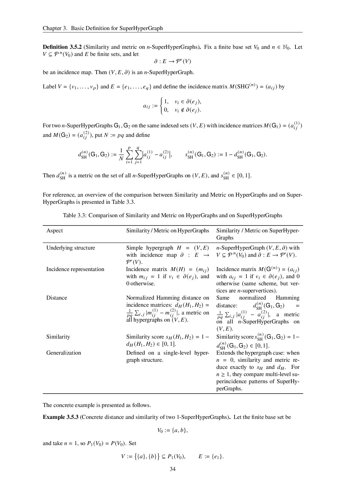
Chapter 3. Basic Definition for SuperHyperGraph Definition 3.5.2 (Similarity and
metric on 𝑛-SuperHyperGraphs). Fix a finite base set 𝑉0 and 𝑛 ∈ N0. Let 𝑉 ⊆ P 𝑛(𝑉0 ) and 𝐸 be finite sets, and let 𝜕 : 𝐸 → P∗(𝑉) be an incidence map. Then (𝑉, 𝐸, 𝜕) is an 𝑛-SuperHyperGraph. Label 𝑉 = {𝑣1, . . . , 𝑣𝑝 } and 𝐸 = {𝑒1, . . . , 𝑒𝑞 } and define the incidence matrix 𝑀(SHG(𝑛)) = (𝑎𝑖 𝑗 ) by 𝑎𝑖 𝑗 := 1, 𝑣𝑖 ∈ 𝜕(𝑒𝑗 ), 0, 𝑣𝑖 ∉ 𝜕(𝑒𝑗 ). For two 𝑛-SuperHyperGraphs G1, G2 on the same indexed sets (𝑉, 𝐸) with incidence matrices 𝑀(G1 ) = (𝑎 (1) 𝑖 𝑗 ) and 𝑀(G2 ) = (𝑎 (2) 𝑖 𝑗 ), put 𝑁 := 𝑝𝑞 and define 𝑑 (𝑛) SH (G1, G2 ) := 1 𝑁 𝑝 ∑︁ 𝑖=1 𝑞 ∑︁ 𝑗=1 𝑎 (1) 𝑖 𝑗 − 𝑎 (2) 𝑖 𝑗 , 𝑠 (𝑛) SH (G1, G2 ) := 1 − 𝑑 (𝑛) SH (G1, G2 ). Then 𝑑 (𝑛) SH is a metric on the set of all 𝑛-SuperHyperGraphs on (𝑉, 𝐸), and 𝑠 (𝑛) SH ∈ [0, 1]. For reference, an overview of the comparison between Similarity and Metric on HyperGraphs and on Super- HyperGraphs is presented in Table 3.3. Table 3.3: Comparison of Similarity and Metric on HyperGraphs and on SuperHyperGraphs Aspect Similarity / Metric on HyperGraphs Similarity / Metric on SuperHyper- Graphs Underlying structure Simple hypergraph 𝐻 = (𝑉, 𝐸) with incidence map 𝜕 : 𝐸 → P∗(𝑉). 𝑛-SuperHyperGraph (𝑉, 𝐸, 𝜕) with 𝑉 ⊆ P 𝑛(𝑉0 ) and 𝜕 : 𝐸 → P∗(𝑉). Incidence representation Incidence matrix 𝑀(𝐻) = (𝑚𝑖 𝑗 ) with 𝑚𝑖 𝑗 = 1 if 𝑣𝑖 ∈ 𝜕(𝑒𝑗 ), and 0 otherwise. Incidence matrix 𝑀(G(𝑛)) = (𝑎𝑖 𝑗 ) with 𝑎𝑖 𝑗 = 1 if 𝑣𝑖 ∈ 𝜕(𝑒𝑗 ), and 0 otherwise (same scheme, but vertices are 𝑛-supervertices). Distance Normalized Hamming distance on incidence matrices: 𝑑𝐻 (𝐻1, 𝐻2 ) = 1 𝑝𝑞 𝑖, 𝑗 |𝑚 (1) 𝑖 𝑗 − 𝑚 (2) 𝑖 𝑗 |, a metric on all hypergraphs on (𝑉, 𝐸). Same normalized Hamming distance: 𝑑 (𝑛) SH (G1, G2 ) = 1 𝑝𝑞 𝑖, 𝑗 |𝑎 (1) 𝑖 𝑗 − 𝑎 (2) 𝑖 𝑗 |, a metric on all 𝑛-SuperHyperGraphs on (𝑉, 𝐸). Similarity Similarity score 𝑠𝐻 (𝐻1, 𝐻2 ) = 1 − 𝑑𝐻 (𝐻1, 𝐻2 ) ∈ [0, 1]. Similarity score 𝑠 (𝑛) SH (G1, G2 ) = 1− 𝑑 (𝑛) SH (G1, G2 ) ∈ [0, 1]. Generalization Defined on a single-level hypergraph structure. Extends the hypergraph case: when 𝑛 = 0, similarity and metric reduce exactly to 𝑠𝐻 and 𝑑𝐻 . For 𝑛 ≥ 1, they compare multi-level superincidence patterns of SuperHy- perGraphs. The concrete example is presented as follows. Example 3.5.3 (Concrete distance and similarity of two 1-SuperHyperGraphs). Let the finite base set be 𝑉0 := {𝑎, 𝑏}, and take 𝑛 = 1, so 𝑃1 (𝑉0 ) = 𝑃(𝑉0 ). Set 𝑉 := {𝑎}, {𝑏} ⊆ 𝑃1 (𝑉0 ), 𝐸 := {𝑒1 }. 34

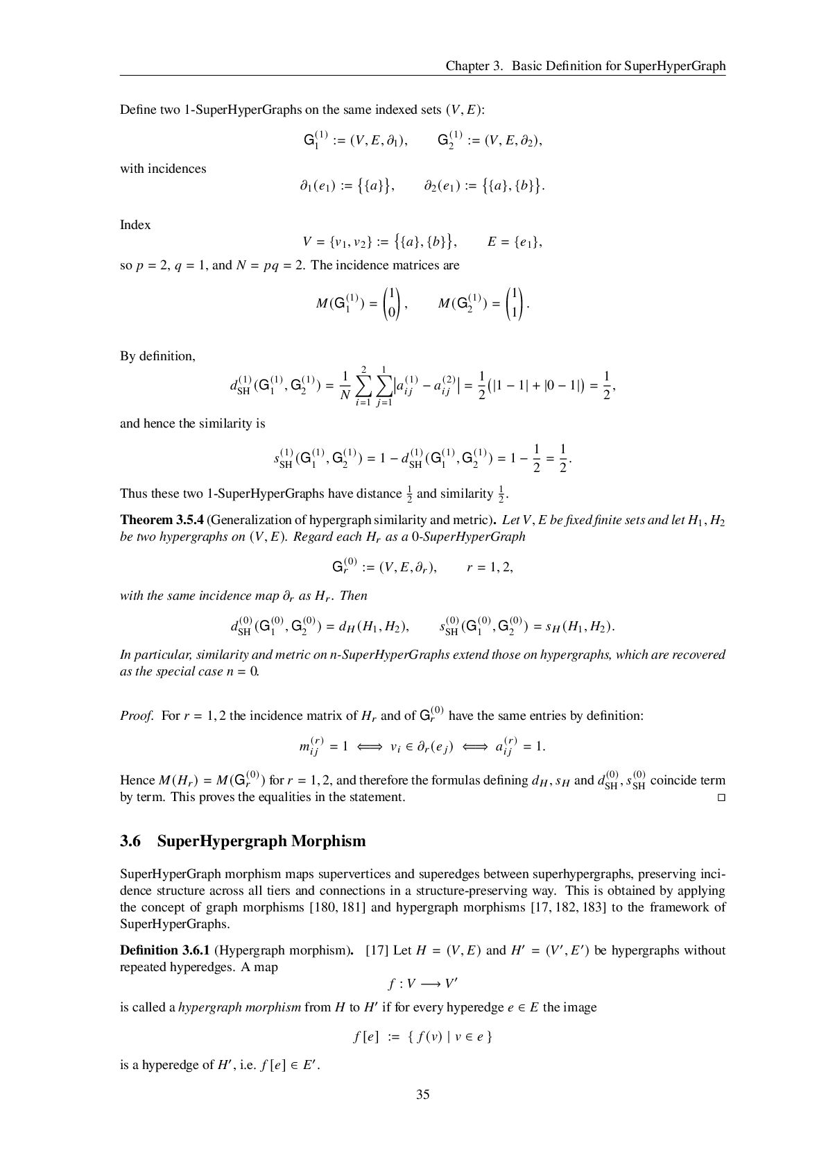
Chapter 3. Basic Definition for SuperHyperGraph Define two 1-SuperHyperGraphs on
the same indexed sets (𝑉, 𝐸): G(1) 1 := (𝑉, 𝐸, 𝜕1 ), G(1) 2 := (𝑉, 𝐸, 𝜕2 ), with incidences 𝜕1 (𝑒1 ) := {𝑎} , 𝜕2 (𝑒1 ) := {𝑎}, {𝑏} . Index 𝑉 = {𝑣1, 𝑣2 } := {𝑎}, {𝑏} , 𝐸 = {𝑒1 }, so 𝑝 = 2, 𝑞 = 1, and 𝑁 = 𝑝𝑞 = 2. The incidence matrices are 𝑀(G(1) 1 ) = 1 0 , 𝑀(G(1) 2 ) = 1 1 . By definition, 𝑑 (1) SH (G(1) 1 , G(1) 2 ) = 1 𝑁 2 ∑︁ 𝑖=1 1 ∑︁ 𝑗=1 𝑎 (1) 𝑖 𝑗 − 𝑎 (2) 𝑖 𝑗 = 1 2 |1 − 1| + |0 − 1| = 1 2, and hence the similarity is 𝑠 (1) SH (G(1) 1 , G(1) 2 ) = 1 − 𝑑 (1) SH (G(1) 1 , G(1) 2 ) = 1 − 1 2 = 1 2. Thus these two 1-SuperHyperGraphs have distance 1 2 and similarity 1 2 . Theorem 3.5.4 (Generalization of hypergraph similarity and metric). Let 𝑉, 𝐸 be fixed finite sets and let 𝐻1, 𝐻2 be two hypergraphs on (𝑉, 𝐸). Regard each 𝐻𝑟 as a 0-SuperHyperGraph G(0) 𝑟 := (𝑉, 𝐸, 𝜕𝑟 ), 𝑟 = 1, 2, with the same incidence map 𝜕𝑟 as 𝐻𝑟 . Then 𝑑 (0) SH (G(0) 1 , G(0) 2 ) = 𝑑𝐻 (𝐻1, 𝐻2 ), 𝑠 (0) SH (G(0) 1 , G(0) 2 ) = 𝑠𝐻 (𝐻1, 𝐻2 ). In particular, similarity and metric on 𝑛-SuperHyperGraphs extend those on hypergraphs, which are recovered as the special case 𝑛 = 0. Proof. For 𝑟 = 1, 2 the incidence matrix of 𝐻𝑟 and of G(0) 𝑟 have the same entries by definition: 𝑚 (𝑟) 𝑖 𝑗 = 1 ⇐⇒ 𝑣𝑖 ∈ 𝜕𝑟 (𝑒𝑗 ) ⇐⇒ 𝑎 (𝑟) 𝑖 𝑗 = 1. Hence 𝑀(𝐻𝑟 ) = 𝑀(G(0) 𝑟 ) for 𝑟 = 1, 2, and therefore the formulas defining 𝑑𝐻, 𝑠𝐻 and 𝑑 (0) SH , 𝑠 (0) SH coincide term by term. This proves the equalities in the statement. □ 3.6 SuperHypergraph Morphism SuperHyperGraph morphism maps supervertices and superedges between superhypergraphs, preserving incidence structure across all tiers and connections in a structure-preserving way. This is obtained by applying the concept of graph morphisms [180, 181] and hypergraph morphisms [17, 182, 183] to the framework of SuperHyperGraphs. Definition 3.6.1 (Hypergraph morphism). [17] Let 𝐻 = (𝑉, 𝐸) and 𝐻′ = (𝑉′ , 𝐸′) be hypergraphs without repeated hyperedges. A map 𝑓 : 𝑉 −→ 𝑉′ is called a hypergraph morphism from 𝐻 to 𝐻′ if for every hyperedge 𝑒 ∈ 𝐸 the image 𝑓 [𝑒] := { 𝑓 (𝑣) | 𝑣 ∈ 𝑒 } is a hyperedge of 𝐻′, i.e. 𝑓 [𝑒] ∈ 𝐸′. 35

Chapter 3. Basic Definition for SuperHyperGraph Definition 3.6.2 (SuperHypergraph morphism).
Let H1 = (𝑉1, 𝐸1, 𝜕1 ) and H2 = (𝑉2, 𝐸2, 𝜕2 ) be SuperHyper- Graphs, where 𝑉𝑖 is the (possibly tiered) supervertex set, 𝐸𝑖 is the set of superedges, and 𝜕𝑖 : 𝐸𝑖 −→ P∗(𝑉𝑖 ) is the incidence map assigning to each superedge a nonempty set of supervertices, with P∗(𝑉𝑖 ) := P(𝑉𝑖 ) \ {∅}. A SuperHyperGraph morphism 𝐹 : H1 −→ H2 is a pair 𝐹 = ( 𝑓 , 𝑔) consisting of 𝑓 : 𝑉1 −→ 𝑉2, 𝑔 : 𝐸1 −→ 𝐸2, such that the following compatibility condition holds for every 𝑒 ∈ 𝐸1: 𝜕2 𝑔(𝑒) = 𝑓# 𝜕1 (𝑒) , where 𝑓# : P(𝑉1 ) −→ P(𝑉2 ), 𝑓# (𝑋) := { 𝑓 (𝑣) | 𝑣 ∈ 𝑋 }, is the direct image map on subsets. Table 3.4 presents a comparison of Hypergraph morphisms and SuperHyperGraph morphisms. Table 3.4: Comparison of Hypergraph morphisms and SuperHyperGraph morphisms Aspect Hypergraph morphism SuperHyperGraph morphism Underlying objects Hypergraphs 𝐻 = (𝑉, 𝐸) and 𝐻′ = (𝑉′ , 𝐸′) without repeated hyperedges. SuperHyperGraphs H1 = (𝑉1, 𝐸1, 𝜕1 ) and H2 = (𝑉2, 𝐸2, 𝜕2 ), where vertices and edges may be tiered. Maps A single vertex map 𝑓 : 𝑉 → 𝑉′. A pair of maps 𝐹 = ( 𝑓 , 𝑔) with 𝑓 : 𝑉1 → 𝑉2 (on supervertices) and 𝑔 : 𝐸1 → 𝐸2 (on superedges). Incidence preservation For every 𝑒 ∈ 𝐸, the image 𝑓 [𝑒] = { 𝑓 (𝑣) | 𝑣 ∈ 𝑒} is required to be a hyperedge of 𝐻′, i.e. 𝑓 [𝑒] ∈ 𝐸′. For every 𝑒 ∈ 𝐸1, the incidence condition 𝜕2 𝑔(𝑒) = 𝑓# 𝜕1 (𝑒) must hold, where 𝑓# (𝑋) = { 𝑓 (𝑣) | 𝑣 ∈ 𝑋}. Level of structure Preserves membership of vertices in hyperedges at a single level. Preserves membership of supervertices in superedges across possibly multi-level superstructures via a compatible pair ( 𝑓 , 𝑔). Reduction Fundamental notion in classical hypergraph theory. Extends the hypergraph case: when supervertices/edges collapse to ordinary vertices/edges, the notion reduces to a hypergraph morphism. Example 3.6.3 (A simple SuperHyperGraph morphism). Let H1 = (𝑉1, 𝐸1, 𝜕1 ) and H2 = (𝑉2, 𝐸2, 𝜕2 ) be SuperHyperGraphs defined by 𝑉1 := {𝑣1, 𝑣2, 𝑣3 }, 𝐸1 := {𝑒1 }, 𝜕1 (𝑒1 ) := {𝑣1, 𝑣2 }, 𝑉2 := {𝑤1, 𝑤2 }, 𝐸2 := { 𝑓1 }, 𝜕2 ( 𝑓1 ) := {𝑤1, 𝑤2 }. Define maps 𝑓 : 𝑉1 → 𝑉2, 𝑓 (𝑣1 ) := 𝑤1, 𝑓 (𝑣2 ) := 𝑤2, 𝑓 (𝑣3 ) := 𝑤2, 𝑔 : 𝐸1 → 𝐸2, 𝑔(𝑒1 ) := 𝑓1. 36

Chapter 3. Basic Definition for SuperHyperGraph The direct image of
the incident set of 𝑒1 is 𝑓# 𝜕1 (𝑒1 ) = 𝑓# ({𝑣1, 𝑣2 }) = { 𝑓 (𝑣1 ), 𝑓 (𝑣2 )} = {𝑤1, 𝑤2 }. Hence 𝜕2 𝑔(𝑒1 ) = 𝜕2 ( 𝑓1 ) = {𝑤1, 𝑤2 } = 𝑓# 𝜕1 (𝑒1 ) , so the pair 𝐹 = ( 𝑓 , 𝑔) is a SuperHyperGraph morphism 𝐹 : H1 −→ H2. Theorem 3.6.4 (SuperHyperGraph morphisms generalize hypergraph morphisms). Let 𝐻 = (𝑉, 𝐸) and 𝐻′ = (𝑉′ , 𝐸′) be hypergraphs without repeated hyperedges, and regard them as SuperHyperGraphs via H = (𝑉, 𝐸, 𝜕), H′ = (𝑉′ , 𝐸′ , 𝜕′), where 𝜕(𝑒) = 𝑒 ⊆ 𝑉, 𝜕′(𝑒′) = 𝑒′ ⊆ 𝑉′ (𝑒 ∈ 𝐸, 𝑒′ ∈ 𝐸′). Then a map 𝑓 : 𝑉 → 𝑉′ is a hypergraph morphism 𝐻 → 𝐻′ if and only if there exists a map 𝑔 : 𝐸 → 𝐸′ such that ( 𝑓 , 𝑔) is a SuperHyperGraph morphism H → H′ in the sense of Definition 3.6.2. Proof. (⇒) Suppose 𝑓 : 𝑉 → 𝑉′ is a hypergraph morphism. For each 𝑒 ∈ 𝐸 the image 𝑓 [𝑒] = { 𝑓 (𝑣) | 𝑣 ∈ 𝑒} is a hyperedge of 𝐻′, so 𝑓 [𝑒] ∈ 𝐸′. Define 𝑔 : 𝐸 → 𝐸′ by 𝑔(𝑒) := 𝑓 [𝑒] ∈ 𝐸′ . Then, for every 𝑒 ∈ 𝐸, 𝜕′ 𝑔(𝑒) = 𝑔(𝑒) = 𝑓 [𝑒] = 𝑓# 𝜕(𝑒) , because 𝜕(𝑒) = 𝑒 and 𝜕′(𝑔(𝑒)) = 𝑔(𝑒) by construction. Hence ( 𝑓 , 𝑔) satisfies the compatibility condition and is a SuperHyperGraph morphism. (⇐) Conversely, assume there exists 𝑔 : 𝐸 → 𝐸′ such that ( 𝑓 , 𝑔) is a SuperHyperGraph morphism. For each 𝑒 ∈ 𝐸 we then have 𝜕′ 𝑔(𝑒) = 𝑓# 𝜕(𝑒) . Using 𝜕(𝑒) = 𝑒 and 𝜕′(𝑔(𝑒)) = 𝑔(𝑒), this becomes 𝑔(𝑒) = 𝑓# (𝑒) = { 𝑓 (𝑣) | 𝑣 ∈ 𝑒}. Thus 𝑓 [𝑒] = 𝑔(𝑒) ∈ 𝐸′, so 𝑓 sends every hyperedge of 𝐻 to a hyperedge of 𝐻′. Therefore 𝑓 is a hypergraph morphism. Consequently, hypergraph morphisms are precisely those vertex maps that admit a completion to a SuperHy- perGraph morphism between the associated SuperHyperGraphs, so the notion of SuperHyperGraph morphism is a genuine generalization of hypergraph morphism. □ 3.7 SuperHyperGraph Partitioning Graph partitioning divides a graph’s vertices into disjoint blocks, minimizing the number (or weight) of edges crossing between different blocks [184]. Related concepts such as Fuzzy Graph Partitioning [185, 186] and Directed Graph Partitioning [187–189] are also well known. Graph partitioning is essential for scalable computation, reducing communication costs, enabling parallelism, improving clustering quality, and accelerating large-scale optimization and learning. Hypergraph partitioning splits vertices into blocks, minimizing cut hyperedges while balancing block sizes, better capturing multiway relationships than standard graph partitioning [190–192]. SuperHyperGraph partitioning divides supervertices and superedges into balanced groups, minimizing cut weight while respecting hierarchical multi-level connectivity constraints and structure [193]. 37

Chapter 3. Basic Definition for SuperHyperGraph Definition 3.7.1 (𝑘-way 𝑛-SuperHyperGraph
partition). [193] Let 𝐻(𝑛) = (𝑉, 𝐸) be an 𝑛-SuperHyperGraph, and let 𝑘 ∈ N, 𝑘 ≥ 2. A 𝑘-way partition of 𝑉 is a family of subsets V := {𝑉1, . . . ,𝑉𝑘 } such that 𝑉𝑖 ⊆ 𝑉, 𝑉𝑖 ∩ 𝑉𝑗 = ∅ (𝑖 ≠ 𝑗), 𝑘 𝑖=1 𝑉𝑖 = 𝑉. Fix a balance parameter 𝑐 ≥ 1. The partition V is called 𝑐-balanced if 1 𝑐 |𝑉| 𝑘 ≤ |𝑉𝑖 | ≤ 𝑐 |𝑉| 𝑘 for all 𝑖 = 1, . . . , 𝑘. For a given partition V and a superedge 𝑒 ∈ 𝐸, define the number of parts spanned by 𝑒 as spanV (𝑒) := { 𝑖 ∈ {1, . . . , 𝑘} | 𝑒 ∩ 𝑉𝑖 ≠ ∅ } . The superedge-cut cost of V is 𝑓cut (V) := ∑︁ 𝑒∈𝐸 spanV (𝑒) − 1 . The 𝑘-way 𝑛-SuperHyperGraph partitioning problem is: given 𝐻(𝑛) = (𝑉, 𝐸), 𝑘, and 𝑐 ≥ 1, find a 𝑐-balanced 𝑘-way partition V = {𝑉1, . . . ,𝑉𝑘 } of 𝑉 that minimizes 𝑓cut (V) (or another chosen objective such as the sum of external degrees). Table 3.5 presents a Comparison of Graph, HyperGraph, and SuperHyperGraph Partitioning. Table 3.5: Comparison of Graph, HyperGraph, and SuperHyperGraph Partitioning Aspect Graph Partitioning HyperGraph Partitioning SuperHyperGraph Parti- tioning Underlying structure Graph 𝐺 = (𝑉, 𝐸) with edges joining two vertices. HyperGraph 𝐻 = (𝑉, 𝐸) with hyperedges 𝑒 ⊆ 𝑉. 𝑛-SuperHyperGraph 𝐻(𝑛) = (𝑉, 𝐸) with supervertices and superedges on iterated powersets. Partition object Vertex set 𝑉 split into disjoint blocks. Vertex set 𝑉 split into disjoint blocks. Supervertex set𝑉 split into disjoint blocks. Cut notion Number or total weight of edges crossing between blocks. Number or total weight of hyperedges incident to more than one block. Superedge-cut cost 𝑓cut (V) = ∑︁ 𝑒∈𝐸 (spanV (𝑒) − 1), measuring how many blocks each superedge spans. Balance constraint Block sizes approximately equal (e.g., bounded ratio to |𝑉|/𝑘). Block sizes approximately equal under a chosen balance parameter. 𝑐-balanced: 1 𝑐 |𝑉| 𝑘 ≤ |𝑉𝑖 | ≤ 𝑐 |𝑉| 𝑘 for all parts 𝑉𝑖 . Goal Minimize edges crossing between blocks while maintaining balance. Minimize cut hyperedges (and possibly their weights) while maintaining balance; better captures multiway relationships. Minimize superedge-cut cost while respecting hierarchical, multi-level connectivity and structural constraints. Hereafter, we present a concrete example. 38

Chapter 3. Basic Definition for SuperHyperGraph Example 3.7.2 (2-way partition
of a small 2-SuperHyperGraph). We give a concrete 2-SuperHyperGraph and an explicit optimal 2-way partition with respect to the cut objective. Base level (individuals). Let 𝑉0 := {𝑎, 𝑏, 𝑐, 𝑑} represent four individual employees. Level 1 (teams). Consider the following nonempty subsets of 𝑉0: 𝑇1 := {𝑎, 𝑏}, 𝑇2 := {𝑏, 𝑐}, 𝑇3 := {𝑐, 𝑑}. Level 2 (departments as sets of teams). Define three departments 𝐷1 := {𝑇1,𝑇2 }, 𝐷2 := {𝑇2,𝑇3 }, 𝐷3 := {𝑇1,𝑇3 }. Each 𝐷𝑖 is a nonempty subset of {𝑇1,𝑇2,𝑇3 }, so 𝐷𝑖 ∈ 𝑃 𝑃(𝑉0 ) = 𝑃2 (𝑉0 ). We set the 2-supervertex set and 2-superedge set as 𝑉 := {𝐷1, 𝐷2, 𝐷3 }, 𝐸 := 𝑒1 := {𝐷1, 𝐷2 }, 𝑒2 := {𝐷2, 𝐷3 } . Then 𝐻(2) = (𝑉, 𝐸) is a finite 2-SuperHyperGraph. We now partition 𝑉 into 𝑘 = 2 parts. Let 𝑉1 := {𝐷1, 𝐷2 }, 𝑉2 := {𝐷3 }. Clearly 𝑉1 ∩ 𝑉2 = ∅ and 𝑉1 ∪ 𝑉2 = 𝑉. Balance check. Here |𝑉| = 3 and 𝑘 = 2, so the ideal size is |𝑉|/𝑘 = 3/2. Choose 𝑐 = 2. Then 1 𝑐 |𝑉| 𝑘 = 1 2 · 3 2 = 3 4, 𝑐 |𝑉| 𝑘 = 2 · 3 2 = 3. We have |𝑉1 | = 2 and |𝑉2 | = 1, so 3 4 ≤ 1 ≤ 3, 3 4 ≤ 2 ≤ 3, hence the partition is 2-balanced. Cut cost. We compute spanV (𝑒) for each superedge 𝑒 ∈ 𝐸, where V = {𝑉1,𝑉2 }. For 𝑒1 = {𝐷1, 𝐷2 } we have 𝑒1 ⊆ 𝑉1, so spanV (𝑒1 ) = 1, spanV (𝑒1 ) − 1 = 0. For 𝑒2 = {𝐷2, 𝐷3 } we have 𝐷2 ∈ 𝑉1 and 𝐷3 ∈ 𝑉2, hence spanV (𝑒2 ) = 2, spanV (𝑒2 ) − 1 = 1. Therefore the total cut cost is 𝑓cut (V) = spanV (𝑒1 ) − 1 + spanV (𝑒2 ) − 1 = 0 + 1 = 1. If we instead consider the alternative partition 𝑉′ 1 := {𝐷1, 𝐷3 }, 𝑉′ 2 := {𝐷2 }, then both superedges span both parts: spanV′ (𝑒1 ) = 2, spanV′ (𝑒2 ) = 2, so 𝑓cut (V′) = (2 − 1) + (2 − 1) = 2. Hence the original partition V = {𝑉1,𝑉2 } is strictly better with respect to the cut objective 𝑓cut. This example shows explicitly how a small 2-SuperHyperGraph can be partitioned into two balanced parts while minimizing the number of superedges that cross between parts. 39

Chapter 3. Basic Definition for SuperHyperGraph 3.8 SuperHyperGraph Coloring Graph
coloring assigns colors to vertices so adjacent vertices differ, modeling resource allocation, scheduling conflicts, or frequency assignment constraints [194–197]. Related concepts such as Fuzzy Graph Coloring [198, 199], Directed Graph Coloring [200–202], Edge Coloring [203,204], Total coloring [205,206], Face coloring [207, 208], and Neutrosophic Graph Coloring [194, 209] are also well known. HyperGraph coloring assigns colors to vertices so no hyperedge is monochromatic, extending classical coloring to multiway interactions and constraints [210–213]. SuperHyperGraph coloring assigns colors to supervertices across iterated powerset levels, preventing monochromatic superedges and capturing hierarchical multi-level conflict structures. Definition 3.8.1 (Hypergraph coloring). [214,215] Let 𝐻 = (𝑉(𝐻), 𝐸(𝐻)) be a finite hypergraph with ∅ ≠ 𝑉(𝐻), ∅ ≠ 𝐸(𝐻) ⊆ P∗ 𝑉(𝐻) , where P∗(𝑋) := P(𝑋) \ {∅}. Let 𝑐 ∈ N with 𝑐 ≥ 1, and let C := {1, 2, . . . , 𝑐} be a set of 𝑐 colors. A 𝑐-coloring of 𝐻 is a function 𝜑 : 𝑉(𝐻) −→ C. Such a coloring 𝜑 is called proper if no hyperedge is monochromatic, that is, ∀ 𝑒 ∈ 𝐸(𝐻) : {𝜑(𝑣) | 𝑣 ∈ 𝑒} ≠ {𝑖} for every 𝑖 ∈ C. Equivalently, every 𝑒 ∈ 𝐸(𝐻) contains at least two vertices with distinct colors. The chromatic number of 𝐻 is 𝜒(𝐻) := min 𝑐 ∈ N | 𝐻 admits a proper 𝑐-coloring . Definition 3.8.2 (SuperHyperGraph coloring). Let SHG(𝑛) = (𝑉𝑛, 𝐸𝑛 ) be an 𝑛-SuperHyperGraph as above. Fix 𝑐 ∈ N with 𝑐 ≥ 1 and a color set C := {1, 2, . . . , 𝑐}. A 𝑐-coloring of the 𝑛-SuperHyperGraph SHG(𝑛) is a function 𝜓 : 𝑉𝑛 −→ C. Such a coloring 𝜓 is called proper if no 𝑛-superedge is monochromatic, that is, ∀ 𝑒 ∈ 𝐸𝑛 : {𝜓(𝑣) | 𝑣 ∈ 𝑒} ≠ {𝑖} for every 𝑖 ∈ C. The SuperHyperGraph chromatic number of SHG(𝑛) is 𝜒 SHG(𝑛) := min 𝑐 ∈ N | SHG(𝑛) admits a proper 𝑐-coloring . Table 3.6 presents an overview of the comparison among Graph Coloring, HyperGraph Coloring, and Super- HyperGraph Coloring. Hereafter, we present a concrete example. 40

Chapter 3. Basic Definition for SuperHyperGraph Table 3.6: Comparison of
Graph Coloring, HyperGraph Coloring, and SuperHyperGraph Coloring Aspect Graph Coloring HyperGraph Coloring SuperHyperGraph Color- ing Underlying structure Graph 𝐺 = (𝑉, 𝐸) with edges joining pairs of vertices. HyperGraph 𝐻 = (𝑉, 𝐸) with hyperedges 𝑒 ⊆ 𝑉. 𝑛-SuperHyperGraph SHG(𝑛) = (𝑉𝑛, 𝐸𝑛 ) on iterated powersets. Coloring object Vertices 𝑉 are colored. Vertices 𝑉 are colored. Supervertices 𝑉𝑛 (collections on higher levels) are colored. Proper-coloring constraint Adjacent vertices must receive different colors; no edge is monochromatic. No hyperedge is monochromatic; every hyperedge contains at least two distinct colors. No 𝑛-superedge is monochromatic; every superedge contains at least two distinct colors at the supervertex level. Chromatic parameter Chromatic number 𝜒(𝐺): minimum number of colors in a proper coloring. Chromatic number 𝜒(𝐻): minimum number of colors in a proper hypergraph coloring. SuperHyperGraph chromatic number 𝜒(SHG(𝑛)): minimum number of colors in a proper 𝑛-SuperHyperGraph coloring. Level of conflict modeled Pairwise conflicts between individual vertices. Multiway conflicts within vertex subsets (hyperedges). Hierarchical multi-level conflicts between supervertices and their superedges. Example 3.8.3 (A 2-colorable SuperHyperGraph). Let 𝑉0 := {𝑣1, 𝑣2, 𝑣3 }, 𝐸0 := {𝑒1, 𝑒2 } with hyperedges 𝑒1 := {𝑣1, 𝑣2 }, 𝑒2 := {𝑣2, 𝑣3 }. Then SHG(0) := (𝑉0, 𝐸0 ) is a 0-SuperHyperGraph. Take 𝑐 = 2 and the color set C := {1, 2}. Define a coloring 𝜓 : 𝑉0 → C by 𝜓(𝑣1 ) := 1, 𝜓(𝑣2 ) := 2, 𝜓(𝑣3 ) := 1. For each 𝑒 ∈ 𝐸0 we have {𝜓(𝑣) | 𝑣 ∈ 𝑒1 } = {𝜓(𝑣1 ), 𝜓(𝑣2 )} = {1, 2}, {𝜓(𝑣) | 𝑣 ∈ 𝑒2 } = {𝜓(𝑣2 ), 𝜓(𝑣3 )} = {1, 2}, so no edge is monochromatic and 𝜓 is a proper 2-coloring. If we tried 𝑐 = 1 and colored all vertices with a single color, then each edge would be monochromatic, so no proper 1-coloring exists. Therefore 𝜒 SHG(0) = 2. Example 3.8.4 (A 3-chromatic 1-SuperHyperGraph). Let the base set be 𝑉0 := {𝑎, 𝑏, 𝑐}. Form three 1-supervertices 𝐴 := {𝑎, 𝑏}, 𝐵 := {𝑏, 𝑐}, 𝐶 := {𝑎, 𝑐}, 41

Chapter 3. Basic Definition for SuperHyperGraph and set 𝑉1 :=
{𝐴, 𝐵, 𝐶}. Define 1-superedges 𝑒1 := {𝐴, 𝐵}, 𝑒2 := {𝐵, 𝐶}, 𝑒3 := {𝐴, 𝐶}, and let 𝐸1 := {𝑒1, 𝑒2, 𝑒3 }. Then SHG(1) := (𝑉1, 𝐸1 ) is a 1-SuperHyperGraph whose underlying structure on the tier-1 vertices 𝐴, 𝐵, 𝐶 is the complete graph 𝐾3. Take 𝑐 = 3 with color set C := {1, 2, 3}, and define 𝜓 : 𝑉1 → C by 𝜓(𝐴) := 1, 𝜓(𝐵) := 2, 𝜓(𝐶) := 3. Then {𝜓(𝑣) | 𝑣 ∈ 𝑒1 } = {𝜓(𝐴), 𝜓(𝐵)} = {1, 2}, {𝜓(𝑣) | 𝑣 ∈ 𝑒2 } = {𝜓(𝐵), 𝜓(𝐶)} = {2, 3}, {𝜓(𝑣) | 𝑣 ∈ 𝑒3 } = {𝜓(𝐴), 𝜓(𝐶)} = {1, 3}, so no 1-superedge is monochromatic and 𝜓 is a proper 3-coloring. On the other hand, any 2-coloring of 𝐴, 𝐵, 𝐶 must assign the same color to some pair, say 𝜓(𝐴) = 𝜓(𝐵). Since {𝐴, 𝐵} is a 1-superedge, this edge would then be monochromatic, contradicting properness. Hence no proper 2-coloring exists and 𝜒 SHG(1) = 3. Theorem 3.8.5 (SuperHyperGraph coloring generalizes hypergraph coloring). Every hypergraph coloring problem is a special case of SuperHyperGraph coloring at level 𝑛 = 0. More precisely, for every finite hypergraph 𝐻 = (𝑉(𝐻), 𝐸(𝐻)) there exists a level-0 SuperHyperGraph SHG(0) = (𝑉0, 𝐸0 ) such that: 1. 𝑉0 = 𝑉(𝐻) and 𝐸0 = 𝐸(𝐻); 2. for every integer 𝑐 ≥ 1, the proper 𝑐-colorings of 𝐻 are exactly the proper 𝑐-colorings of SHG(0) (via the same vertex-coloring functions); 3. in particular, 𝜒 𝐻 = 𝜒 SHG(0) . Proof. Let 𝐻 = (𝑉(𝐻), 𝐸(𝐻)) be a finite hypergraph. Set 𝑉0 := 𝑉(𝐻), 𝐸0 := 𝐸(𝐻). Recall that by definition P0 (𝑉0 ) = 𝑉0, P∗(𝑉0 ) = P(𝑉0 ) \ {∅}. Since 𝐸(𝐻) ⊆ P∗ 𝑉(𝐻) = P∗(𝑉0 ), the pair SHG(0) := (𝑉0, 𝐸0 ) satisfies ∅ ≠ 𝑉0 ⊆ P0 (𝑉0 ), ∅ ≠ 𝐸0 ⊆ P∗(𝑉0 ), so it is a level-0 SuperHyperGraph on the base set 𝑉0. Fix 𝑐 ∈ N, 𝑐 ≥ 1, and let C = {1, . . . , 𝑐} be the set of colors. 42

Chapter 3. Basic Definition for SuperHyperGraph (1) Suppose first that
𝜑 : 𝑉(𝐻) → C is a proper hypergraph 𝑐-coloring of 𝐻. Define 𝜓 : 𝑉0 −→ C, 𝜓(𝑣) := 𝜑(𝑣) (𝑣 ∈ 𝑉0 ). Since 𝑉0 = 𝑉(𝐻) and 𝐸0 = 𝐸(𝐻), for every edge 𝑒 ∈ 𝐸0 we have {𝜓(𝑣) | 𝑣 ∈ 𝑒} = {𝜑(𝑣) | 𝑣 ∈ 𝑒}. Because 𝜑 is proper on 𝐻, no 𝑒 ∈ 𝐸(𝐻) = 𝐸0 is monochromatic under 𝜑, hence no 𝑒 ∈ 𝐸0 is monochromatic under 𝜓. Thus 𝜓 is a proper 𝑐-coloring of the level-0 SuperHyperGraph SHG(0). (2) Conversely, suppose that 𝜓 : 𝑉0 → C is a proper 𝑐-coloring of SHG(0). Define 𝜑 : 𝑉(𝐻) −→ C, 𝜑(𝑣) := 𝜓(𝑣) (𝑣 ∈ 𝑉(𝐻) = 𝑉0 ). For every hyperedge 𝑒 ∈ 𝐸(𝐻) = 𝐸0 we again have {𝜑(𝑣) | 𝑣 ∈ 𝑒} = {𝜓(𝑣) | 𝑣 ∈ 𝑒}. Since 𝜓 is proper on SHG(0), no 𝑒 ∈ 𝐸0 is monochromatic under 𝜓, hence no 𝑒 ∈ 𝐸(𝐻) is monochromatic under 𝜑. Therefore 𝜑 is a proper 𝑐-coloring of the original hypergraph 𝐻. The constructions in (1) and (2) are inverses of each other (they are both the identity map on the underlying set 𝑉(𝐻) = 𝑉0). Thus, for every 𝑐 ≥ 1, there is a natural bijection proper 𝑐-colorings of 𝐻 proper 𝑐-colorings of SHG(0) . Taking the minimum 𝑐 for which these sets are nonempty on each side, we obtain 𝜒(𝐻) = 𝜒 SHG(0) . Hence hypergraph coloring is realized exactly as the special case 𝑛 = 0 of SuperHyperGraph coloring, which proves that SuperHyperGraph coloring is a proper generalization of hypergraph coloring. □ 3.9 SuperHyperGraph Domination Graph domination investigates subsets of vertices such that every vertex either belongs to the subset or is adjacent to at least one vertex in it, with a primary focus on minimizing the size of such subsets in graphs [216–218]. Related notions of domination and its variants have also been extensively studied in the settings of fuzzy graphs and neutrosophic graphs (e.g., [219–222]). In addition, several well-known variants of domination exist, including secure domination [223, 224], paired domination [225, 226], double domination [227, 228], roman domination [229–231], connected domination [232–234], star domination [235–237], and total domination [238]. Hypergraph domination extends graph domination by requiring that each vertex outside a dominating set shares at least one hyperedge with a dominating vertex, thereby modeling influence coverage in more complex multiway interaction systems [239–242]. SuperHyperGraph domination further generalizes hypergraph domination to multi-tier supervertices, by requiring that every supervertex is connected, via at least one superedge, to some dominating supervertex while respecting the hierarchical structure across the superhypergraph levels. Definition 3.9.1 (Domination in a hypergraph). (cf. [239–241, 243]) Let 𝐻 = (𝑉, 𝐸) be a finite hypergraph with nonempty vertex set 𝑉 and hyperedge family 𝐸 ⊆ P∗(𝑉) := P(𝑉) \ {∅}. A subset 𝐷 ⊆ 𝑉 is called a dominating set of 𝐻 if for every vertex 𝑣 ∈ 𝑉 \ 𝐷 there exists an edge 𝑒 ∈ 𝐸 such that 𝑣 ∈ 𝑒 and 𝑒 ∩ 𝐷 ≠ ∅. Equivalently, every vertex outside 𝐷 is contained in some edge that also contains at least one vertex of 𝐷. The domination number of 𝐻 is 𝛾(𝐻) := min{ |𝐷| | 𝐷 ⊆ 𝑉 is a dominating set of 𝐻 }. 43

Chapter 3. Basic Definition for SuperHyperGraph Example 3.9.2 (Domination in
a small hypergraph). Consider the hypergraph 𝐻 = (𝑉, 𝐸) with vertex set 𝑉 := {1, 2, 3, 4} and hyperedge family 𝐸 := 𝑒1, 𝑒2, 𝑒3 := {1, 2}, {2, 3}, {3, 4} . Define 𝐷 := {2, 3} ⊆ 𝑉. We check that 𝐷 is a dominating set of 𝐻. For each vertex 𝑣 ∈ 𝑉 \ 𝐷 = {1, 4}: • 𝑣 = 1: we have 1 ∈ 𝑒1 = {1, 2} and 𝑒1 ∩ 𝐷 = {2} ≠ ∅. • 𝑣 = 4: we have 4 ∈ 𝑒3 = {3, 4} and 𝑒3 ∩ 𝐷 = {3} ≠ ∅. Thus every vertex outside 𝐷 lies in some hyperedge that also contains a vertex from 𝐷, so 𝐷 is dominating. No singleton {1}, {2}, {3}, or {4} is dominating: • {1} fails to dominate 4, • {2} fails to dominate 4, • {3} fails to dominate 1, • {4} fails to dominate 1. Hence no dominating set of size 1 exists, and the domination number is 𝛾(𝐻) = 2. Definition 3.9.3(Domination in an 𝑛-SuperHyperGraph). (cf. [112]) Let SHG(𝑛) = (𝑉, 𝐸) be an 𝑛-SuperHyperGraph on a finite base set 𝑉0. A subset 𝐷 ⊆ 𝑉 is called a dominating set of SHG(𝑛) if for every 𝑛-supervertex 𝑣 ∈ 𝑉 \ 𝐷 there exists an 𝑛-superedge 𝑒 ∈ 𝐸 such that 𝑣 ∈ 𝑒 and 𝑒 ∩ 𝐷 ≠ ∅. Equivalently, every 𝑛-supervertex outside 𝐷 lies in some 𝑛-superedge that also contains at least one 𝑛- supervertex from 𝐷. The domination number of SHG(𝑛) is 𝛾 SHG(𝑛) := min{ |𝐷| | 𝐷 ⊆ 𝑉 is a dominating set of SHG(𝑛) }. Table 3.7 provides an overview of the comparison between graph, hypergraph, and superhypergraph domination. Hereafter, we present a concrete example. 44

Chapter 3. Basic Definition for SuperHyperGraph Table 3.7: Comparison of
graph, hypergraph, and superhypergraph domination Framework Underlying structure Domination condition Graph domination Vertices joined by ordinary edges; adjacency is pairwise between vertices. A set 𝐷 ⊆ 𝑉 such that every 𝑣 ∈ 𝑉 \ 𝐷 is adjacent to at least one vertex in 𝐷. HyperGraph domination Vertices joined by hyperedges; each hyperedge is a nonempty subset of 𝑉. A set 𝐷 ⊆ 𝑉 such that for every 𝑣 ∈ 𝑉 \ 𝐷 there exists a hyperedge 𝑒 with 𝑣 ∈ 𝑒 and 𝑒 ∩ 𝐷 ≠ ∅. SuperHyperGraph domination 𝑛-supervertices 𝑉 ⊆ P𝑛(𝑉0 ) joined by 𝑛-superedges (images of the incidence map). A set 𝐷 ⊆ 𝑉 such that for every 𝑣 ∈ 𝑉\𝐷 there exists an 𝑛-superedge 𝑒 with 𝑣 ∈ 𝑒 and 𝑒 ∩ 𝐷 ≠ ∅, respecting the hierarchical supervertex structure. Example 3.9.4 (Domination in a 1-SuperHyperGraph). Let the base set be 𝑉0 := {𝑎, 𝑏, 𝑐}. Form three 1-supervertices 𝐴 := {𝑎, 𝑏}, 𝐵 := {𝑏, 𝑐}, 𝐶 := {𝑎, 𝑐}, and set 𝑉 := {𝐴, 𝐵, 𝐶}. Define two 1-superedges 𝑒1 := {𝐴, 𝐵}, 𝑒2 := {𝐵, 𝐶}, and let 𝐸 := {𝑒1, 𝑒2 }. Then SHG(1) := (𝑉, 𝐸) is a 1-SuperHyperGraph. Consider the subset 𝐷 := {𝐵} ⊆ 𝑉. We verify that 𝐷 is a dominating set of SHG(1). For each 1-supervertex 𝑣 ∈ 𝑉 \ 𝐷 = {𝐴, 𝐶}: • 𝑣 = 𝐴: we have 𝐴 ∈ 𝑒1 = {𝐴, 𝐵} and 𝑒1 ∩ 𝐷 = {𝐵} ≠ ∅. • 𝑣 = 𝐶: we have 𝐶 ∈ 𝑒2 = {𝐵, 𝐶} and 𝑒2 ∩ 𝐷 = {𝐵} ≠ ∅. Thus every 1-supervertex outside 𝐷 belongs to some 1-superedge that also contains an element of 𝐷, so 𝐷 is dominating. No dominating set of size 0 exists, so 𝐷 is a minimum dominating set and the domination number is 𝛾 SHG(1) = 1. Theorem 3.9.5 (SuperHyperGraph domination generalizes hypergraph domination). Every finite hypergraph can be viewed as a 0-SuperHyperGraph in such a way that dominating sets (and hence the domination number) coincide. In particular, hypergraph domination is a special case of 𝑛-SuperHyperGraph domination (for 𝑛 = 0). 45

Chapter 3. Basic Definition for SuperHyperGraph Proof. Let 𝐻 =
(𝑉, 𝐸) be an arbitrary finite hypergraph with ∅ ≠ 𝑉 and ∅ ≠ 𝐸 ⊆ P∗(𝑉). Take the base set𝑉0 := 𝑉 and consider the 0-fold iterated powerset P0(𝑉0 ) = 𝑉0. Define the 0-SuperHyperGraph SHG(0) 𝐻 := (𝑉 (0) , 𝐸(0)) by 𝑉 (0) := 𝑉, 𝐸(0) := 𝐸. Since 𝐸(0) ⊆ P∗(𝑉 (0)) and 𝑉 (0) ⊆ P0(𝑉0 ), this is a valid 0-SuperHyperGraph on the base set 𝑉0 in the sense of the previous definition. We now compare dominating sets. Let 𝐷 ⊆ 𝑉. (i) Suppose 𝐷 is a dominating set of 𝐻. By definition of hypergraph domination, for every vertex 𝑣 ∈ 𝑉 \ 𝐷 there exists an edge 𝑒 ∈ 𝐸 such that 𝑣 ∈ 𝑒 and 𝑒 ∩ 𝐷 ≠ ∅. But 𝐸(0) = 𝐸 and 𝑉 (0) = 𝑉, so the same condition reads: for every 𝑣 ∈ 𝑉 (0) \ 𝐷 there exists 𝑒 ∈ 𝐸(0) with 𝑣 ∈ 𝑒 and 𝑒 ∩ 𝐷 ≠ ∅. This is exactly the condition that 𝐷 is a dominating set of SHG(0) 𝐻 . (ii) Conversely, suppose 𝐷 ⊆ 𝑉 (0) = 𝑉 is a dominating set of SHG(0) 𝐻 . By definition of 0-SuperHyperGraph domination, for every 𝑣 ∈ 𝑉 (0) \ 𝐷 there exists 𝑒 ∈ 𝐸(0) such that 𝑣 ∈ 𝑒 and 𝑒 ∩ 𝐷 ≠ ∅. Since 𝐸(0) = 𝐸, this is exactly the condition that 𝐷 is a dominating set of the original hypergraph 𝐻. Thus { 𝐷 ⊆ 𝑉 | 𝐷 dominates 𝐻 } = { 𝐷 ⊆ 𝑉 (0) | 𝐷 dominates SHG(0) 𝐻 }. Taking minima of the cardinalities of dominating sets on both sides, we obtain 𝛾(𝐻) = 𝛾 SHG(0) 𝐻 . Therefore every hypergraph domination problem can be regarded as a special case of 𝑛-SuperHyperGraph domination (with 𝑛 = 0), and SuperHyperGraph domination strictly generalizes hypergraph domination. □ 3.10 Sombor index of SuperHypergraphs Sombor index of a graph sums, over edges, the square root of squared endpoint degrees, capturing degree-based structural complexity information [244–246]. These concepts have been further extended and studied in various settings, including chemical graphs [247, 248], fuzzy graphs [249, 250], and neutrosophic graphs [251, 252]. Moreover, related concepts such as the modified Sombor index [253–255], the Zagreb index [256–258], the Hyper-Zagreb Index [259,260], the ABC index [261,262], and the GA index [263,264] are also well known. Sombor index of a hypergraph generalizes this by summing square-rooted degree squares over each hyperedge’s incident vertices within complex interactions [265]. Sombor index of a superhypergraph extends further, aggregating degree-squared contributions over multi-tier superedges, reflecting hierarchical connectivity across nested structural levels. Definition 3.10.1 (Sombor index of a hypergraph). [265] Let 𝐻 = (𝑉, 𝐸) be a finite hypergraph, where 𝑉 is a nonempty finite vertex set and 𝐸 ⊆ P∗(𝑉) is a finite family of nonempty subsets of 𝑉 (the hyperedges). For each vertex 𝑣 ∈ 𝑉, the degree of 𝑣 in 𝐻 is 𝑑𝐻 (𝑣) := { 𝑒 ∈ 𝐸 | 𝑣 ∈ 𝑒 } . 46

Chapter 3. Basic Definition for SuperHyperGraph The Sombor index of
the hypergraph 𝐻 is defined by 𝑆𝑂(𝐻) := ∑︁ 𝑒∈𝐸 √︄ ∑︁ 𝑣∈𝑒 𝑑𝐻 (𝑣)2 . When 𝐻 is 2-uniform (i.e., every hyperedge has size 2), this reduces to the classical Sombor index of a simple graph. Example 3.10.2 (Sombor index of a small hypergraph). Consider the hypergraph 𝐻 = (𝑉, 𝐸), where the vertex set and hyperedge family are 𝑉 := {𝑥, 𝑦, 𝑧}, 𝐸 := {𝑒1, 𝑒2, 𝑒3 }, with 𝑒1 := {𝑥, 𝑦}, 𝑒2 := {𝑦, 𝑧}, 𝑒3 := {𝑥, 𝑦, 𝑧}. This is a non–2-uniform hypergraph (since |𝑒3 | = 3). Step 1: Vertex degrees. For each 𝑣 ∈ 𝑉, the degree 𝑑𝐻 (𝑣) := |{𝑒 ∈ 𝐸 | 𝑣 ∈ 𝑒}| is: 𝑑𝐻 (𝑥) = 2 (appears in 𝑒1, 𝑒3), 𝑑𝐻 (𝑦) = 3 (appears in 𝑒1, 𝑒2, 𝑒3), 𝑑𝐻 (𝑧) = 2 (appears in 𝑒2, 𝑒3). Step 2: Sombor index. By definition, 𝑆𝑂(𝐻) := ∑︁ 𝑒∈𝐸 √︄ ∑︁ 𝑣∈𝑒 𝑑𝐻 (𝑣)2 . We compute the contribution of each hyperedge. For 𝑒1 = {𝑥, 𝑦}: ∑︁ 𝑣∈𝑒1 𝑑𝐻 (𝑣)2 = 𝑑𝐻 (𝑥)2 + 𝑑𝐻 (𝑦)2 = 22 + 32 = 4 + 9 = 13, so the contribution of 𝑒1 is √ 13. For 𝑒2 = {𝑦, 𝑧}: ∑︁ 𝑣∈𝑒2 𝑑𝐻 (𝑣)2 = 𝑑𝐻 (𝑦)2 + 𝑑𝐻 (𝑧)2 = 32 + 22 = 9 + 4 = 13, so the contribution of 𝑒2 is also √ 13. For 𝑒3 = {𝑥, 𝑦, 𝑧}: ∑︁ 𝑣∈𝑒3 𝑑𝐻 (𝑣)2 = 𝑑𝐻 (𝑥)2 + 𝑑𝐻 (𝑦)2 + 𝑑𝐻 (𝑧)2 = 22 + 32 + 22 = 4 + 9 + 4 = 17, so the contribution of 𝑒3 is √ 17. Therefore, the Sombor index of 𝐻 is 𝑆𝑂(𝐻) = √ 13 + √ 13 + √ 17 = 2 √ 13 + √ 17. In this example, the presence of a 3-vertex hyperedge 𝑒3 shows how the Sombor index naturally extends beyond the graph (2-uniform) case. 47

Chapter 3. Basic Definition for SuperHyperGraph Definition 3.10.3 (Degree in
an 𝑛-SuperHyperGraph). Let SHG(𝑛) = (𝑉, 𝐸, 𝜕) be a level-𝑛 SuperHyperGraph. For each 𝑣 ∈ 𝑉, the degree of 𝑣 in SHG(𝑛) is 𝑑SHG(𝑛) (𝑣) := { 𝑒 ∈ 𝐸 | 𝑣 ∈ 𝜕(𝑒) } . Definition 3.10.4 (Sombor index of an 𝑛-SuperHyperGraph). Let SHG(𝑛) = (𝑉, 𝐸, 𝜕) be a level-𝑛 SuperHy- perGraph. The Sombor index of SHG(𝑛) is defined by 𝑆𝑂 SHG(𝑛) := ∑︁ 𝑒∈𝐸 √︄ ∑︁ 𝑣∈𝜕(𝑒) 𝑑SHG(𝑛) (𝑣)2 . Remark 3.10.5. If we view a hypergraph 𝐻 = (𝑉, 𝐸) in incidence form by taking 𝜕(𝑒) = 𝑒 for all 𝑒 ∈ 𝐸, then the above formula coincides with the Sombor index of a hypergraph. Table 3.8 provides an overview of the comparison of the Sombor index for graphs, hypergraphs, and superhypergraphs. Table 3.8: Comparison of Sombor index for graphs, hypergraphs, and superhypergraphs Framework Underlying structure Sombor index Graph Simple graph 𝐺 = (𝑉, 𝐸) with pairwise edges between vertices. 𝑆𝑂(𝐺) = ∑︁ 𝑢𝑣∈𝐸 √︁ 𝑑𝐺 (𝑢)2 + 𝑑𝐺 (𝑣)2. Hypergraph Hypergraph 𝐻 = (𝑉, 𝐸) where each hyperedge 𝑒 ∈ 𝐸 is a nonempty subset of 𝑉. 𝑆𝑂(𝐻) = ∑︁ 𝑒∈𝐸 √︄∑︁ 𝑣∈𝑒 𝑑𝐻 (𝑣)2. SuperHypergraph Level-𝑛 SuperHyperGraph SHG(𝑛) = (𝑉, 𝐸, 𝜕) with 𝑛-supervertices and 𝑛- superedges. 𝑆𝑂 SHG(𝑛) = ∑︁ 𝑒∈𝐸 √︄ ∑︁ 𝑣∈𝜕(𝑒) 𝑑SHG(𝑛) (𝑣)2. Example 3.10.6 (Sombor index of a 1-SuperHyperGraph with two tiers). We now consider a simple 1- SuperHyperGraph that mixes base vertices and 1-supervertices. Step 1: Vertex sets and supervertices. Let the base set be 𝑉0 := {𝑎, 𝑏, 𝑐}. Form two first-tier (super)vertices 𝑃 := {𝑎, 𝑏}, 𝑄 := {𝑏, 𝑐}, and set 𝑉1 := {𝑃, 𝑄}. The total vertex set is 𝑉 := 𝑉0 ∪ 𝑉1 = {𝑎, 𝑏, 𝑐, 𝑃, 𝑄}. Step 2: Superedges and boundary map. Define three superedges 𝐸 := {𝑒1, 𝑒2, 𝑒3 }, with boundary map 𝜕 : 𝐸 → P∗(𝑉) given by 𝜕(𝑒1 ) := {𝑎, 𝑃}, 𝜕(𝑒2 ) := {𝑏, 𝑃, 𝑄}, 𝜕(𝑒3 ) := {𝑐, 𝑄}. Thus SHG(1) := (𝑉, 𝐸, 𝜕) is a level-1 SuperHyperGraph: 𝑎, 𝑏, 𝑐 are base vertices, 𝑃, 𝑄 are 1-supervertices, and each superedge connects a small subset of these across tiers. 48

Chapter 3. Basic Definition for SuperHyperGraph Step 3: Vertex degrees
in SHG(1). For 𝑣 ∈ 𝑉, the degree 𝑑SHG(1) (𝑣) := {𝑒 ∈ 𝐸 | 𝑣 ∈ 𝜕(𝑒)} is: 𝑑SHG(1) (𝑎) = 1 (only in 𝜕(𝑒1 )), 𝑑SHG(1) (𝑏) = 1 (only in 𝜕(𝑒2 )), 𝑑SHG(1) (𝑐) = 1 (only in 𝜕(𝑒3 )), 𝑑SHG(1) (𝑃) = 2 (in 𝜕(𝑒1 ) and 𝜕(𝑒2 )), 𝑑SHG(1) (𝑄) = 2 (in 𝜕(𝑒2 ) and 𝜕(𝑒3 )). Step 4: Sombor index of the 1-SuperHyperGraph. By definition, 𝑆𝑂 SHG(1) := ∑︁ 𝑒∈𝐸 √︄ ∑︁ 𝑣∈𝜕(𝑒) 𝑑SHG(1) (𝑣)2 . We compute each term. For 𝑒1 with 𝜕(𝑒1 ) = {𝑎, 𝑃}: ∑︁ 𝑣∈𝜕(𝑒1 ) 𝑑SHG(1) (𝑣)2 = 𝑑SHG(1) (𝑎)2 + 𝑑SHG(1) (𝑃)2 = 12 + 22 = 1 + 4 = 5, so the contribution of 𝑒1 is √ 5. For 𝑒2 with 𝜕(𝑒2 ) = {𝑏, 𝑃, 𝑄}: ∑︁ 𝑣∈𝜕(𝑒2 ) 𝑑SHG(1) (𝑣)2 = 𝑑SHG(1) (𝑏)2 + 𝑑SHG(1) (𝑃)2 + 𝑑SHG(1) (𝑄)2 = 12 + 22 + 22 = 1 + 4 + 4 = 9, so the contribution of 𝑒2 is √ 9 = 3. For 𝑒3 with 𝜕(𝑒3 ) = {𝑐, 𝑄}: ∑︁ 𝑣∈𝜕(𝑒3 ) 𝑑SHG(1) (𝑣)2 = 𝑑SHG(1) (𝑐)2 + 𝑑SHG(1) (𝑄)2 = 12 + 22 = 1 + 4 = 5, so the contribution of 𝑒3 is √ 5. Therefore, the Sombor index of the 1-SuperHyperGraph is 𝑆𝑂 SHG(1) = √ 5 + 3 + √ 5 = 2 √ 5 + 3. In this example, the Sombor index incorporates both base vertices (𝑎, 𝑏, 𝑐) and higher-tier supervertices (𝑃, 𝑄), reflecting how hierarchical incidences in a SuperHyperGraph contribute jointly to the overall index. 49

Chapter 3. Basic Definition for SuperHyperGraph Theorem 3.10.7 (SuperHyperGraph Sombor
index generalises the hypergraph Sombor index). Let 𝐻 = (𝑉, 𝐸) be a finite hypergraph. Define the associated level-0 SuperHyperGraph SHG(0) 𝐻 := (𝑉, 𝐸, 𝜕𝐻 ), 𝜕𝐻 (𝑒) := 𝑒 (𝑒 ∈ 𝐸). Then 𝑆𝑂 SHG(0) 𝐻 = 𝑆𝑂(𝐻). In particular, the Sombor index of an 𝑛-SuperHyperGraph is a strict extension of the Sombor index of a hypergraph (the case 𝑛 = 0). Proof. By construction, 𝑉 is the vertex set of both 𝐻 and SHG(0) 𝐻 , and 𝐸 is the edge/superedge set in both structures. For every vertex 𝑣 ∈ 𝑉 we have 𝑑SHG(0) 𝐻 (𝑣) = { 𝑒 ∈ 𝐸 | 𝑣 ∈ 𝜕𝐻 (𝑒) } = { 𝑒 ∈ 𝐸 | 𝑣 ∈ 𝑒 } = 𝑑𝐻 (𝑣). Thus the degree of each vertex is identical in 𝐻 and in SHG(0) 𝐻 . Next, for every edge 𝑒 ∈ 𝐸 we have 𝜕𝐻 (𝑒) = 𝑒, so the inner sum in the SuperHyperGraph Sombor index is ∑︁ 𝑣∈𝜕𝐻 (𝑒) 𝑑SHG(0) 𝐻 (𝑣)2 = ∑︁ 𝑣∈𝑒 𝑑𝐻 (𝑣)2 . Therefore 𝑆𝑂 SHG(0) 𝐻 = ∑︁ 𝑒∈𝐸 √︄ ∑︁ 𝑣∈𝜕𝐻 (𝑒) 𝑑SHG(0) 𝐻 (𝑣)2 = ∑︁ 𝑒∈𝐸 √︄ ∑︁ 𝑣∈𝑒 𝑑𝐻 (𝑣)2 = 𝑆𝑂(𝐻). Hence the Sombor index of an 𝑛-SuperHyperGraph extends the Sombor index of a hypergraph, and the latter is recovered exactly when we restrict to level 𝑛 = 0 with 𝜕(𝑒) = 𝑒. □ 3.11 SuperHyperGraph Labeling Graph labeling assigns labels to a graph’s vertices and/or edges so that specified constraints hold, typically driven by adjacency, incidence, or distances [266–268]. As related concepts in graph labeling, graceful labeling [269,270], magic labeling [271,272], harmonious labeling [273,274], and lucky labeling [275,276] are well known. Graph labeling has also been studied within the frameworks of fuzzy graphs, neutrosophic graphs, and related generalized graph models (e.g., [277–280]). Hypergraph labeling assigns labels to vertices and/or hyperedges so that incidence-based or overlap-based constraints are satisfied across the hypergraph structure [281–283]. SuperHyperGraph labeling assigns labels to 𝑛-supervertices and/or n-superedges so that constraints respect the super-incidence structure induced at level 𝑛 [284]. SuperHyperGraph multilabeling assigns several label components to each supervertex and/or superedge, requiring these components to satisfy coupled constraints and remain consistent [284]. Definition 3.11.1 (Graph Labeling). [266–268] Let 𝐺 = (𝑉, 𝐸) be a finite graph and let 𝐿𝑉 and 𝐿𝐸 be nonempty label alphabets. A (possibly partial) graph labeling on 𝐺 consists of maps ℓ𝑉 : 𝑉 → 𝐿𝑉 and/or ℓ𝐸 : 𝐸 → 𝐿𝐸, where either map may be omitted if not used. A labeling schema is a predicate Φ(𝐺; ℓ𝑉 , ℓ𝐸 ) built from adjacency/incidence in 𝐺, the graph distance dist𝐺 on 𝑉, and fixed relations/operations on the alphabets (e.g. =, ≠, order, arithmetic, etc.). We call (ℓ𝑉 , ℓ𝐸 ) valid (for Φ) if Φ(𝐺; ℓ𝑉 , ℓ𝐸 ) holds. Example 3.11.2 (An 𝐿(2, 1) vertex-labeling on the path 𝑃5). Let 𝑃5 have vertices 𝑣1, 𝑣2, 𝑣3, 𝑣4, 𝑣5 and edges 𝑣𝑖𝑣𝑖+1 for 𝑖 = 1, 2, 3, 4. Let 𝐿𝑉 = Z and define a vertex labeling ℓ𝑉 : 𝑉(𝑃5 ) → Z by ℓ𝑉 (𝑣1 ) = 0, ℓ𝑉 (𝑣2 ) = 2, ℓ𝑉 (𝑣3 ) = 4, ℓ𝑉 (𝑣4 ) = 1, ℓ𝑉 (𝑣5 ) = 3. 50

Chapter 3. Basic Definition for SuperHyperGraph Let Φ encode the
𝐿(2, 1) constraints: dist𝑃5 (𝑢, 𝑣) = 1 ⇒ |ℓ𝑉 (𝑢) − ℓ𝑉 (𝑣)| ≥ 2, dist𝑃5 (𝑢, 𝑣) = 2 ⇒ |ℓ𝑉 (𝑢) − ℓ𝑉 (𝑣)| ≥ 1. Verification (distance 1): |0 − 2| = 2, |2 − 4| = 2, |4 − 1| = 3, |1 − 3| = 2. Verification (distance 2): |0 − 4| = 4, |2 − 1| = 1, |4 − 3| = 1. Hence Φ(𝑃5; ℓ𝑉 , ∅) holds, so ℓ𝑉 is a valid 𝐿(2, 1) graph labeling. Definition 3.11.3 (HyperGraph Labeling). [281–283] Let 𝐻 = (𝑉, 𝐸) be a finite hypergraph with 𝐸 ⊆ P(𝑉) \ {∅}, and let 𝐿𝑉 , 𝐿𝐸 be nonempty alphabets. A (possibly partial) hypergraph labeling consists of maps ℓ𝑉 : 𝑉 → 𝐿𝑉 and/or ℓ𝐸 : 𝐸 → 𝐿𝐸 . Write 𝐺(𝐻) for the primal (2-section) graph of 𝐻 on vertex set 𝑉, where {𝑢, 𝑣} is an edge of 𝐺(𝐻) iff 𝑢 ≠ 𝑣 and ∃𝑒 ∈ 𝐸 with {𝑢, 𝑣} ⊆ 𝑒. Let dist𝐻 denote the usual graph distance in 𝐺(𝐻). A labeling schema is a predicate Φ(𝐻; ℓ𝑉 , ℓ𝐸 ) built from the incidence relation 𝑣 ∈ 𝑒, the distance dist𝐻 on 𝑉, and fixed relations/operations on the alphabets. We call (ℓ𝑉 , ℓ𝐸 ) valid if Φ(𝐻; ℓ𝑉 , ℓ𝐸 ) holds. Example 3.11.4 (Strong hyperedge coloring as a hypergraph labeling). Let𝑉 = {1, 2, 3, 4} and let 𝐸 = {𝑒1, 𝑒2 } with 𝑒1 = {1, 2, 3}, 𝑒2 = {3, 4}. Take 𝐿𝑉 = {𝑟, 𝑔, 𝑏} (colors) and define ℓ𝑉 by ℓ𝑉 (1) = 𝑟, ℓ𝑉 (2) = 𝑔, ℓ𝑉 (3) = 𝑏, ℓ𝑉 (4) = 𝑟. Let Φ require strong hyperedge coloring: for every hyperedge 𝑒 ∈ 𝐸, the set {ℓ𝑉 (𝑣) : 𝑣 ∈ 𝑒} is pairwise distinct. Then for 𝑒1 we have {𝑟, 𝑔, 𝑏} (all distinct), and for 𝑒2 we have {𝑏, 𝑟} (distinct). Hence Φ(𝐻; ℓ𝑉 , ∅) holds, so ℓ𝑉 is a valid hypergraph labeling. Definition 3.11.5 (SuperHyperGraph Labeling). [284] Fix 𝑛 ∈ N0 and a finite base set 𝑉0. Write P0(𝑉0 ) = 𝑉0 and P𝑘+1(𝑉0 ) = P(P𝑘 (𝑉0 )). An 𝑛-SuperHyperGraph is a pair SHG(𝑛) = (𝑉, 𝐸) where 𝑉 ⊆ P𝑛(𝑉0 ), ∅ ≠ 𝐸 ⊆ P(𝑉) \ {∅}. Its primal (2-section) graph is 𝐺(SHG(𝑛)) = (𝑉, 𝐸′) where {𝑋,𝑌} ∈ 𝐸′ iff 𝑋 ≠ 𝑌 and ∃𝐹 ∈ 𝐸 with {𝑋,𝑌} ⊆ 𝐹. Let distSHG be the graph distance in 𝐺(SHG(𝑛)). Let 𝐿𝑉 , 𝐿𝐸 be nonempty alphabets. A (possibly partial) SuperHyperGraph labeling consists of maps ℓ𝑉 : 𝑉 → 𝐿𝑉 and/or ℓ𝐸 : 𝐸 → 𝐿𝐸 . A labeling schema is a predicate Φ(SHG(𝑛); ℓ𝑉 , ℓ𝐸 ) built from: the incidence relation 𝑋 ∈ 𝐹 (supervertex– superedge), the distance distSHG on 𝑉, and the set-membership relations available inside P𝑘 (𝑉0 ) for 0 ≤ 𝑘 ≤ 𝑛 (e.g. 𝑥 ∈ 𝑋 when 𝑋 ∈ P(𝑉0 )). We call (ℓ𝑉 , ℓ𝐸 ) valid if Φ(SHG(𝑛); ℓ𝑉 , ℓ𝐸 ) holds. Example 3.11.6 (An 𝐿(2, 1) vertex-labeling on a level-𝑛 = 1 SuperHyperGraph). Let 𝑉0 = {𝑎, 𝑏, 𝑐, 𝑑} and 𝑛 = 1. Define supervertices (elements of P(𝑉0 )): 𝐴 = {𝑎, 𝑏}, 𝐵 = {𝑏, 𝑐}, 𝐶 = {𝑐, 𝑑}, 𝐷 = {𝑎, 𝑑}, and let 𝑉 = {𝐴, 𝐵, 𝐶, 𝐷}. Define superedges (nonempty subsets of 𝑉): 𝐹1 = {𝐴, 𝐵, 𝐶}, 𝐹2 = {𝐴, 𝐷}, and set SHG(1) = (𝑉, 𝐸) with 𝐸 = {𝐹1, 𝐹2 }. Take 𝐿𝑉 = Z and define ℓ𝑉 : 𝑉 → Z by ℓ𝑉 (𝐴) = 0, ℓ𝑉 (𝐵) = 2, ℓ𝑉 (𝐶) = 4, ℓ𝑉 (𝐷) = 3. 51

Chapter 3. Basic Definition for SuperHyperGraph Let Φ encode 𝐿(2,
1) constraints using distSHG: distSHG (𝑋,𝑌) = 1 ⇒ |ℓ𝑉 (𝑋) − ℓ𝑉 (𝑌)| ≥ 2, distSHG (𝑋,𝑌) = 2 ⇒ |ℓ𝑉 (𝑋) − ℓ𝑉 (𝑌)| ≥ 1. In the primal graph, 𝐴 is adjacent to 𝐵, 𝐶, 𝐷 and 𝐵 is adjacent to 𝐶 (via 𝐹1), so |0 − 2| = 2, |0 − 4| = 4, |0 − 3| = 3, |2 − 4| = 2 for all distance-1 pairs, and distSHG (𝐷, 𝐵) = 2, |3 − 2| = 1; distSHG (𝐷, 𝐶) = 2, |3 − 4| = 1. Hence Φ(SHG(1); ℓ𝑉 , ∅) holds, so ℓ𝑉 is a valid SuperHyperGraph labeling. Definition 3.11.7 (SuperHyperGraph MultiLabeling). [284] Let SHG(𝑛) = (𝑉, 𝐸) be an 𝑛-SuperHyperGraph over a base set 𝑉0. Define the flattening (base support) maps ♭𝑛 : P𝑛(𝑉0 ) → P(𝑉0 ) recursively by ♭0 (𝑥) = 𝑥 (𝑥 ∈ 𝑉0 ), ♭𝑘+1 (𝑋) = 𝑌 ∈𝑋 ♭𝑘 (𝑌) (𝑋 ∈ P𝑘+1(𝑉0 )). Thus ♭𝑛 (𝑋) ⊆ 𝑉0 is the set of base elements that occur inside the 𝑛-level object 𝑋. Fix nonnegative integers 𝑝, 𝑞 and choose nonempty alphabets 𝐿 (1) 𝑉 , . . . , 𝐿 ( 𝑝) 𝑉 , 𝐿 (1) 𝐸 , . . . , 𝐿 (𝑞) 𝐸 . A SuperHyperGraph MultiLabeling on SHG(𝑛) consists of coordinate maps ℓ (𝑎) 𝑉 : 𝑉 → 𝐿 (𝑎) 𝑉 (1 ≤ 𝑎 ≤ 𝑝), ℓ (𝑏) 𝐸 : 𝐸 → 𝐿 (𝑏) 𝐸 (1 ≤ 𝑏 ≤ 𝑞), equivalently ℓ𝑉 : 𝑉 → 𝑝 𝑎=1 𝐿 (𝑎) 𝑉 and ℓ𝐸 : 𝐸 → 𝑞 𝑏=1 𝐿 (𝑏) 𝐸 . A multilabeling schema is a predicate Φ(SHG(𝑛); ℓ𝑉 , ℓ𝐸 ) built from the incidence relation 𝑋 ∈ 𝐹, the primal distance distSHG on 𝑉, the membership relations inside P𝑘 (𝑉0 ) (0 ≤ 𝑘 ≤ 𝑛), and the flattening operator ♭𝑛 (plus fixed relations/operations on the alphabets). We call (ℓ𝑉 , ℓ𝐸 ) valid if Φ(SHG(𝑛); ℓ𝑉 , ℓ𝐸 ) holds. Example 3.11.8 (A distance-aware (𝑝, 𝑞) = (2, 1) multilabel on a level-𝑛 = 1 SuperHyperGraph). Let 𝑉0 = {𝑎, 𝑏, 𝑐, 𝑑} and 𝑛 = 1. Define supervertices 𝑋1 = {𝑎, 𝑏}, 𝑋2 = {𝑏, 𝑐}, 𝑋3 = {𝑐, 𝑑}, set 𝑉 = {𝑋1, 𝑋2, 𝑋3 }, and define superedges 𝐹1 = {𝑋1, 𝑋2 }, 𝐹2 = {𝑋2, 𝑋3 }, so SHG(1) = (𝑉, 𝐸) with 𝐸 = {𝐹1, 𝐹2 }. In the primal graph we have distSHG (𝑋1, 𝑋2 ) = 1, distSHG (𝑋2, 𝑋3 ) = 1, and distSHG (𝑋1, 𝑋3 ) = 2. Take alphabets 𝐿 (1) 𝑉 = Z, 𝐿 (2) 𝑉 = N, and 𝐿 (1) 𝐸 = N. Define the coordinate maps by ℓ (1) 𝑉 (𝑋1 ) = 0, ℓ (1) 𝑉 (𝑋2 ) = 2, ℓ (1) 𝑉 (𝑋3 ) = 4, ℓ (2) 𝑉 (𝑋1 ) = 2, ℓ (2) 𝑉 (𝑋2 ) = 2, ℓ (2) 𝑉 (𝑋3 ) = 2, ℓ (1) 𝐸 (𝐹1 ) = 1, ℓ (1) 𝐸 (𝐹2 ) = 1. Let Φ require the following three constraints: (L2,1) distSHG (𝑋,𝑌) = 1 ⇒ |ℓ (1) 𝑉 (𝑋) − ℓ (1) 𝑉 (𝑌)| ≥ 2, distSHG (𝑋,𝑌) = 2 ⇒ |ℓ (1) 𝑉 (𝑋) − ℓ (1) 𝑉 (𝑌)| ≥ 1; (Sup) ℓ (2) 𝑉 (𝑋) = |♭1 (𝑋)| for all 𝑋 ∈ 𝑉; (Int) ℓ (1) 𝐸 (𝐹) = 𝑋∈𝐹 ♭1 (𝑋) for all 𝐹 ∈ 𝐸. Verification: |ℓ (1) 𝑉 (𝑋1 ) − ℓ (1) 𝑉 (𝑋2 )| = |0 − 2| = 2, |ℓ (1) 𝑉 (𝑋2 ) − ℓ (1) 𝑉 (𝑋3 )| = |2 − 4| = 2, |0 − 4| = 4 (dist = 2), and ♭1 (𝑋1 ) = {𝑎, 𝑏}, ♭1 (𝑋2 ) = {𝑏, 𝑐}, ♭1 (𝑋3 ) = {𝑐, 𝑑}, so |♭1 (𝑋𝑖 )| = 2 for all 𝑖, and |♭1 (𝑋1 ) ∩ ♭1 (𝑋2 )| = |{𝑏}| = 1 = ℓ (1) 𝐸 (𝐹1 ), |♭1 (𝑋2 ) ∩ ♭1 (𝑋3 )| = |{𝑐}| = 1 = ℓ (1) 𝐸 (𝐹2 ). Hence Φ(SHG(1); ℓ𝑉 , ℓ𝐸 ) holds, so (ℓ𝑉 , ℓ𝐸 ) is a valid SuperHyperGraph MultiLabeling. 52

Chapter 3. Basic Definition for SuperHyperGraph 3.12 SuperHyperGraph Grammar A
graph grammar rewrites labeled rank-two edges by replacement graphs, gluing two ordered attachment vertices, generating terminal graphs [285, 286]. Related concepts such as fuzzy graph grammars [287–289], digraph grammars [290,291], attributed graph grammars [292,293], and molecular graph grammars [294,295] are also known. A hypergraph grammar rewrites labeled hyperedges of arity r(A) by replacement hypergraphs, identifying ordered attachment tuples, generating terminals [296–298]. A superhypergraph grammar rewrites labeled superhyperedges by ranked n-superhypergraphs with port orderings, gluing external vertices, producing terminal superhypergraphs. Definition 3.12.1 (Ranked hypergraphs in ordered attachment form). Let Σ be a set of edge labels equipped with an arity map 𝑟 : Σ → N≥1. A ranked Σ-hypergraph is a tuple 𝐻 = (𝑉, 𝐸, lab, att) where 𝑉 is a finite vertex set, 𝐸 is a finite edge set, lab : 𝐸 → Σ, and att(𝑒) = (𝑣1, . . . , 𝑣𝑟 (lab(𝑒))) ∈ 𝑉 𝑟 (lab(𝑒)) is the ordered attachment tuple of 𝑒. Definition 3.12.2 (Graph grammar (rank-2 hyperedge replacement)). Let Σ = 𝑁 ∪ 𝑇 be a disjoint union of nonterminals 𝑁 and terminals 𝑇, with arity map 𝑟 : Σ → N≥1 satisfying 𝑟(𝑎) = 2 for all 𝑎 ∈ Σ. A graph grammar (hyperedge-replacement, rank 2) is a tuple G 𝐺 = (𝑁,𝑇, 𝑆, 𝑃) where 𝑆 ∈ 𝑁 and each production is 𝐴 ⇒ 𝑅 with 𝐴 ∈ 𝑁 and 𝑅 a ranked Σ-hypergraph together with an ordered list of external vertices ext(𝑅) = (𝑢1, 𝑢2 ) ∈ 𝑉(𝑅)2 . A derivation starts from the single-edge handle of 𝑆 and repeatedly replaces a nonterminal edge labeled 𝐴 by a fresh copy of 𝑅, identifying the two attachment vertices of the replaced edge with 𝑢1, 𝑢2, and deleting the replaced edge. The language 𝐿(G 𝐺 ) is the set of terminal graphs obtained. Definition 3.12.3 (Hypergraph grammar (hyperedge replacement)). Let Σ = 𝑁 ∪ 𝑇 be a disjoint union, with arity map 𝑟 : Σ → N≥1. A hypergraph grammar (hyperedge-replacement) is a tuple G 𝐻 = (𝑁,𝑇, 𝑆, 𝑃) where 𝑆 ∈ 𝑁 and each production is 𝐴 ⇒ 𝑅 with 𝐴 ∈ 𝑁 and 𝑅 a ranked Σ-hypergraph equipped with an ordered list of external vertices ext(𝑅) = (𝑢1, . . . , 𝑢𝑟 (𝐴)) ∈ 𝑉(𝑅) 𝑟 (𝐴) . A derivation starts from the single-edge handle of 𝑆 and repeatedly replaces a nonterminal edge 𝑒 labeled 𝐴 (with attachment tuple (𝑥1, . . . , 𝑥𝑟 (𝐴))) by a fresh copy of 𝑅, identifying 𝑢𝑖 with 𝑥𝑖 for all 𝑖, and deleting 𝑒. The language 𝐿(G 𝐻 ) is the set of terminal hypergraphs obtained. Definition 3.12.4 (Ranked 𝑛-superhypergraphs with ports). Fix 𝑛 ∈ N0, a base set 𝑉0, a label set Σ and an arity map 𝑟 : Σ → N≥1. A ranked 𝑛-superhypergraph is a tuple S = (𝑉, 𝐸, lab, 𝜕, port) such that (𝑉, 𝐸, 𝜕) is an 𝑛-SuperHyperGraph over 𝑉0, lab : 𝐸 → Σ, and for each 𝑒 ∈ 𝐸 we have a bijection (a port-ordering) port 𝑒 : [𝑟(lab(𝑒))] − − → 𝜕(𝑒). Equivalently, each edge has an ordered attachment tuple att(𝑒) = (port 𝑒 (1), . . . , port 𝑒 (𝑟(lab(𝑒)))). Example 3.12.5 (A hypergraph grammar generating all finite loose paths (rank 2)). Let Σ = 𝑁 ∪ 𝑇 where 𝑁 = {𝐴} and 𝑇 = {𝑡}, and let the arity map be 𝑟(𝐴) = 2, 𝑟(𝑡) = 2. 53

Chapter 3. Basic Definition for SuperHyperGraph We define a hyperedge-replacement
hypergraph grammar G 𝐻 = (𝑁,𝑇, 𝑆, 𝑃) with 𝑆 := 𝐴. Intuitively, terminals 𝑡 will form a loose path of 2-edges (i.e., an ordinary path graph seen as a 2-uniform hypergraph). A derivation starts from the handle consisting of one nonterminal edge labeled 𝐴. Define two productions (both of rank 2): (1) Stop (produce one terminal edge). 𝐴 ⇒ 𝑅stop, where 𝑅stop is the ranked hypergraph with vertex set 𝑉(𝑅stop ) = {𝑢1, 𝑢2 }, edge set 𝐸(𝑅stop ) = {𝑒}, label lab(𝑒) = 𝑡, attachment att(𝑒) = (𝑢1, 𝑢2 ), and externals ext(𝑅stop ) = (𝑢1, 𝑢2 ). (2) Extend (add one terminal edge and keep one nonterminal for further growth). 𝐴 ⇒ 𝑅ext, where 𝑅ext has vertex set 𝑉(𝑅ext ) = {𝑢1, 𝑢2, 𝑤}, edge set 𝐸(𝑅ext ) = {𝑒1, 𝑒2 }, labels lab(𝑒1 ) = 𝑡, lab(𝑒2 ) = 𝐴, attachments att(𝑒1 ) = (𝑢1, 𝑤), att(𝑒2 ) = (𝑤, 𝑢2 ), and externals ext(𝑅ext ) = (𝑢1, 𝑢2 ). Then 𝐿(G 𝐻 ) is exactly the set of finite loose paths: each derivation applies 𝑅ext some number of times and finally applies 𝑅stop, yielding a terminal 2-uniform hypergraph whose hyperedges form a path. Definition 3.12.6 (𝑛-SuperHyperGraph grammar (superhyperedge replacement)). Let 𝑛 ∈ N0, let Σ = 𝑁 ∪ 𝑇 be a disjoint union with arity map 𝑟, and fix a base set 𝑉0. An 𝑛-superhypergraph grammar is a tuple G(𝑛) 𝑆 = (𝑁,𝑇, 𝑆, 𝑃;𝑉0 ) where 𝑆 ∈ 𝑁 and each production is 𝐴 ⇒ 𝑅 with 𝐴 ∈ 𝑁 and 𝑅 = (𝑉𝑅, 𝐸𝑅, lab𝑅, 𝜕𝑅, port𝑅) a ranked 𝑛-superhypergraph together with an ordered list of external vertices ext(𝑅) = (𝑢1, . . . , 𝑢𝑟 (𝐴)) ∈ 𝑉 𝑟 (𝐴) 𝑅 . A derivation starts from the single-edge handle of 𝑆 (as a ranked 𝑛-superhypergraph) and repeatedly: choose a nonterminal edge 𝑒 labeled 𝐴 with ordered attachment tuple (𝑥1, . . . , 𝑥𝑟 (𝐴)), take a fresh copy of 𝑅, identify 𝑢𝑖 with 𝑥𝑖 for all 𝑖 ∈ [𝑟(𝐴)], and delete 𝑒. The language 𝐿(G(𝑛) 𝑆 ) is the set of terminal 𝑛-superhypergraphs obtained. 54

Chapter 3. Basic Definition for SuperHyperGraph Example 3.12.7 (A 2-SuperHyperGraph
grammar generating a chain of supervertices (rank 2)). Fix a base set 𝑉0 := {𝑎, 𝑏, 𝑐}, 𝑛 = 2. Define the level-2 supervertex set (each element is a subset of P(𝑉0 ), hence lies in P2(𝑉0 )) 𝑝𝑎 := {𝑎}, 𝑝𝑏 := {𝑏}, 𝑝𝑐 := {𝑐}, 𝑣𝐿 := {𝑝𝑎 }, 𝑣𝑀 := {𝑝𝑏 }, 𝑣𝑅 := {𝑝𝑐 }, 𝑉 := {𝑣𝐿, 𝑣𝑀, 𝑣𝑅 } ⊆ P2(𝑉0 ). Let Σ = 𝑁 ∪ 𝑇 with 𝑁 = {𝐴}, 𝑇 = {𝑡}, and arities 𝑟(𝐴) = 2, 𝑟(𝑡) = 2. We define a 2-superhypergraph grammar G(2) 𝑆 = (𝑁,𝑇, 𝑆, 𝑃;𝑉0 ) with 𝑆 := 𝐴. We specify two productions 𝐴 ⇒ 𝑅stop and 𝐴 ⇒ 𝑅ext. In both, the external list has length 2 and the port maps impose an order on each (super)edge incidence set. (1) Stop. Let 𝑅stop = (𝑉𝑅, 𝐸𝑅, lab𝑅, 𝜕𝑅, port𝑅) where 𝑉𝑅 = {𝑣𝐿, 𝑣𝑅 }, 𝐸𝑅 = {𝑒}, lab𝑅 (𝑒) = 𝑡, 𝜕𝑅 (𝑒) = {𝑣𝐿, 𝑣𝑅 }, port𝑅 𝑒 (1) = 𝑣𝐿, port𝑅 𝑒 (2) = 𝑣𝑅, and ext(𝑅stop ) = (𝑣𝐿, 𝑣𝑅 ). Thus 𝑅stop produces one terminal superedge connecting the two external supervertices. (2) Extend. Let 𝑅ext = (𝑉𝑅, 𝐸𝑅, lab𝑅, 𝜕𝑅, port𝑅) where 𝑉𝑅 = {𝑣𝐿, 𝑣𝑀, 𝑣𝑅 }, 𝐸𝑅 = {𝑒1, 𝑒2 }, lab𝑅 (𝑒1 ) = 𝑡, lab𝑅 (𝑒2 ) = 𝐴, 𝜕𝑅 (𝑒1 ) = {𝑣𝐿, 𝑣𝑀 }, 𝜕𝑅 (𝑒2 ) = {𝑣𝑀, 𝑣𝑅 }, port𝑅 𝑒1 (1) = 𝑣𝐿, port𝑅 𝑒1 (2) = 𝑣𝑀, port𝑅 𝑒2 (1) = 𝑣𝑀, port𝑅 𝑒2 (2) = 𝑣𝑅, and ext(𝑅ext ) = (𝑣𝐿, 𝑣𝑅 ). Starting from the single-edge handle of 𝑆 = 𝐴, repeated application of 𝑅ext inserts a new intermediate supervertex (a fresh copy of 𝑣𝑀 ) and a terminal superedge to its left, while keeping a nonterminal superedge to the right. A final application of 𝑅stop terminates the derivation. Hence 𝐿(G(2) 𝑆 ) consists of terminal 2-superhypergraphs whose terminal superedges labeled 𝑡 form a (super)edge-chain between the two original external supervertices. Theorem 3.12.8 (𝑛-superhypergraph grammars generalize hypergraph grammars). Let G 𝐻 = (𝑁,𝑇, 𝑆, 𝑃) be a hypergraph grammar over (Σ, 𝑟). (i) For 𝑛 = 0, there exists a 0-superhypergraph grammar G(0) 𝑆 such that (up to the notational identification of hypergraphs with 0-SuperHyperGraphs) 𝐿(G(0) 𝑆 ) = 𝐿(G 𝐻 ). (ii) More generally, for any 𝑛 ∈ N0 there exists an 𝑛-superhypergraph grammar G(𝑛) 𝑆 and an embedding 𝜄𝑛 from terminal hypergraphs to terminal 𝑛-superhypergraphs such that 𝐿(G(𝑛) 𝑆 ) = 𝜄𝑛 𝐿(G 𝐻 ) . 55

Chapter 3. Basic Definition for SuperHyperGraph Proof. (i) View every
ranked Σ-hypergraph 𝐻 = (𝑉, 𝐸, lab, att) as a ranked 0-superhypergraph S(𝐻) = (𝑉, 𝐸, lab, 𝜕, port) over base set 𝑉0 := 𝑉, defined by 𝜕(𝑒) := {𝑣1, . . . , 𝑣𝑟 (lab(𝑒)) } if att(𝑒) = (𝑣1, . . . , 𝑣𝑟 (lab(𝑒))), and port 𝑒 (𝑖) := 𝑣𝑖 for each 𝑖. This is well-defined because 𝑉 ⊆ P0(𝑉0 ) = 𝑉0 and 𝜕(𝑒) ∈ P∗(𝑉). Now define G(0) 𝑆 to have the same 𝑁,𝑇, 𝑆, 𝑃, but interpret every right-hand side 𝑅 of a rule 𝐴 ⇒ 𝑅 as S(𝑅) and keep the same external list. A single replacement step in G 𝐻 replaces an edge with attachment tuple (𝑥1, . . . , 𝑥𝑟 (𝐴)) by gluing the external vertices (𝑢1, . . . , 𝑢𝑟 (𝐴)) of 𝑅 onto that tuple. Because S(·) preserves the ordered attachment tuple via the port maps, the same gluing and deletion operation is exactly a replacement step in G(0) 𝑆 . Hence derivations correspond step-by-step, and terminal objects coincide (up to the identification above), so 𝐿(G(0) 𝑆 ) = 𝐿(G 𝐻 ). (ii) Fix 𝑛 ∈ N0 and define the 𝑛-fold singleton nesting map 𝑠𝑛 : 𝑉0 → P𝑛(𝑉0 ) by 𝑠0 (𝑣) := 𝑣, 𝑠𝑘+1 (𝑣) := {𝑠𝑘 (𝑣)} (𝑘 ≥ 0). Given a ranked Σ-hypergraph 𝐻 = (𝑉, 𝐸, lab, att), define 𝜄𝑛 (𝐻) := 𝑉′ , 𝐸, lab, 𝜕′ , port′ where 𝑉′ := {𝑠𝑛 (𝑣) : 𝑣 ∈ 𝑉} ⊆ P𝑛(𝑉0 ) (choose 𝑉0 to contain all vertex names used), and for each edge 𝑒 with att(𝑒) = (𝑣1, . . . , 𝑣𝑟 (lab(𝑒))) set 𝜕′(𝑒) := {𝑠𝑛 (𝑣1 ), . . . , 𝑠𝑛 (𝑣𝑟 (lab(𝑒)))}, port′ 𝑒 (𝑖) := 𝑠𝑛 (𝑣𝑖 ). Thus 𝜄𝑛 (𝐻) is a ranked 𝑛-superhypergraph and preserves attachment order. Construct G(𝑛) 𝑆 from G 𝐻 by applying 𝜄𝑛 to every right-hand side 𝑅 of a production 𝐴 ⇒ 𝑅, and by applying 𝑠𝑛 to the external vertex list: if ext(𝑅) = (𝑢1, . . . , 𝑢𝑟 (𝐴)), set ext(𝜄𝑛 (𝑅)) = (𝑠𝑛 (𝑢1 ), . . . , 𝑠𝑛 (𝑢𝑟 (𝐴))). Now check one-step rewriting: replacing a nonterminal edge 𝑒 in a sentential form identifies its attachment vertices (𝑥1, . . . , 𝑥𝑟 (𝐴)) with the external vertices of the chosen rule. Since 𝜄𝑛 maps each attachment vertex 𝑥𝑖 to 𝑠𝑛 (𝑥𝑖 ) and each external vertex 𝑢𝑖 to 𝑠𝑛 (𝑢𝑖 ), the identifications commute with 𝜄𝑛 : 𝑠𝑛 (𝑢𝑖 ) identified with 𝑠𝑛 (𝑥𝑖 ) ⇐⇒ 𝑢𝑖 identified with 𝑥𝑖. Therefore, applying a rule in G 𝐻 and then embedding by 𝜄𝑛 yields the same result as first embedding the sentential form and then applying the corresponding rule in G(𝑛) 𝑆 . By induction on the length of derivations, terminal derivations correspond, and terminal languages satisfy 𝐿(G(𝑛) 𝑆 ) = 𝜄𝑛 (𝐿(G 𝐻 )). □ 56

Chapter 4 Some Particular SuperHyperGraphs In graph theory and hypergraph
theory, many graph classes have been studied extensively. Here, a graph class is a family of graphs defined by shared properties or constraints, typically closed under specified operations, which enables systematic analysis and the design of algorithms [299]. Studying graph classes reveals structural patterns, yields efficient algorithms for restricted inputs, clarifies complexity boundaries, and enables transfer- able theorems across graphs sharing forbidden substructures. In this chapter, we present the description and formulation of several particular types of SuperHyperGraphs. 4.1 Directed SuperHyperGraph As discussed above, graphs are widely applied across numerous domains. However, when modeling concepts that inherently involve directional information, the use of directed graphs becomes essential [300,301]. Several extensions of directed graphs are known, including fuzzy directed graphs [302], intuitionistic fuzzy directed graphs [303], rough directed graphs [304], soft directed graphs [305, 306], and neutrosophic directed graphs [307–309]. These structures have been further extended to directed hypergraphs [310–312] and directed superhypergraphs [73,313,314], which have attracted growing research interest. Definition 4.1.1 (Directed Hypergraph). (cf. [315,316]) A directed hypergraph is a pair 𝐻 = (𝑉, 𝐸), where • 𝑉 is a finite set of vertices. • 𝐸 is a finite set of hyperarcs, each hyperarc 𝑒 ∈ 𝐸 being an ordered pair 𝑒 = 𝑇(𝑒), 𝐻(𝑒) ∈ P(𝑉) × P(𝑉), with 𝑇(𝑒) ⊆ 𝑉, 𝑇(𝑒) ≠ ∅, 𝐻(𝑒) ⊆ 𝑉, 𝐻(𝑒) ≠ ∅. Intuitively, each 𝑒 = (𝑇(𝑒), 𝐻(𝑒)) carries “flow” from all vertices in 𝑇(𝑒) (the tail) to all vertices in 𝐻(𝑒) (the head). Example 4.1.2 (A simple directed hypergraph: project dependency flow). Consider the finite vertex set 𝑉 := {Spec, Design, Implement, Test}, representing the phases of a software project: Specification, Design, Implementation, and Testing. Define the set of hyperarcs 𝐸 by 𝐸 := {𝑒1, 𝑒2 }, 57

Chapter 4. Some Particular SuperHyperGraphs where 𝑒1 := 𝑇(𝑒1 ),
𝐻(𝑒1 ) := {Spec}, {Design, Implement} , 𝑒2 := 𝑇(𝑒2 ), 𝐻(𝑒2 ) := {Design, Implement}, {Test} . Then 𝐻 := (𝑉, 𝐸) is a directed hypergraph in the sense of Definition 4.1.1. The hyperarc 𝑒1 models that once the specification is completed, both Design and Implementation can start, while 𝑒2 models that Testing starts only after both Design and Implementation are available. Definition 4.1.3 (Directed 𝑛-SuperHyperGraph). (cf. [2,73]) Let 𝑆 be a nonempty base set and let 𝑛 ≥ 0 be an integer. Define iterated powersets by P0(𝑆) = 𝑆, P𝑘+1(𝑆) = P P𝑘 (𝑆) (𝑘 ≥ 0). A directed 𝑛-SuperHyperGraph is a pair DSHG(𝑛) = (𝑉, 𝐸), where 𝑉 ⊆ P𝑛(𝑆), 𝐸 ⊆ P𝑛(𝑆) × P𝑛(𝑆), and each directed 𝑛-superedge 𝑒 ∈ 𝐸 is an ordered pair 𝑒 = Tail(𝑒), Head(𝑒) , Tail(𝑒), Head(𝑒) ⊆ P𝑛(𝑆), typically both nonempty. Such an 𝑒 carries “flow” from the entire set Tail(𝑒) of 𝑛-supervertices into Head(𝑒). Example 4.1.4 (A simple directed 1-SuperHyperGraph: information flow between groups). Let the base set of individuals be 𝑆 := {𝑢1, 𝑢2, 𝑢3, 𝑢4 }, so that P0(𝑆) = 𝑆, P1(𝑆) = P(𝑆). We construct a directed 1-SuperHyperGraph, where each vertex is a group of individuals. Define the set of 1-supervertices 𝑉 := 𝐴 := {𝑢1, 𝑢2 }, 𝐵 := {𝑢2, 𝑢3, 𝑢4 }, 𝐶 := {𝑢3 } ⊆ P1(𝑆), and the set of directed 1-superedges 𝐸 := {𝑒1, 𝑒2 } ⊆ P1(𝑆) × P1(𝑆), where 𝑒1 := Tail(𝑒1 ), Head(𝑒1 ) := {𝐴}, {𝐵} , 𝑒2 := Tail(𝑒2 ), Head(𝑒2 ) := {𝐵}, {𝐶} . Then DSHG(1) := (𝑉, 𝐸) is a directed 1-SuperHyperGraph in the sense of Definition 4.1.3 with 𝑛 = 1. Here, 𝑒1 represents information flowing from the group {𝑢1, 𝑢2 } to the larger group {𝑢2, 𝑢3, 𝑢4 }, and 𝑒2 represents subsequent forwarding from {𝑢2, 𝑢3, 𝑢4 } to the single individual {𝑢3 }. For reference, Table 4.1 provides information comparing directed graphs, directed hypergraphs, and directed 𝑛-SuperHyperGraphs. 58

Chapter 4. Some Particular SuperHyperGraphs Table 4.1: Comparison of directed
graphs, directed hypergraphs, and directed 𝑛-SuperHyperGraphs Framework Vertices Directed edge / arc structure Directed graph Finite vertex set 𝑉. Arc set 𝐴 ⊆ 𝑉 ×𝑉; each arc (𝑢, 𝑣) carries direction from 𝑢 (tail) to 𝑣 (head). Directed hypergraph Finite vertex set 𝑉. Hyperarc set 𝐸, each 𝑒 ∈ 𝐸 is an ordered pair (𝑇(𝑒), 𝐻(𝑒)) with nonempty 𝑇(𝑒), 𝐻(𝑒) ⊆ 𝑉; direction flows from all 𝑇(𝑒) to all 𝐻(𝑒). Directed 𝑛- SuperHyperGraph 𝑛-supervertex set 𝑉 ⊆ P𝑛(𝑆) over a base set 𝑆. Directed 𝑛-superedge set 𝐸 ⊆ P𝑛(𝑆)× P𝑛(𝑆); each 𝑒 = (Tail(𝑒), Head(𝑒)) carries flow from a family of 𝑛- supervertices to another, across hierarchical levels. 4.2 Bidirected SuperHyperGraph One of the well-known extended notions of a directed graph is the bidirected graph. A bidirected graph assigns to each vertex–edge incidence a sign indicating whether the edge is locally directed toward or away from that vertex [317–320]. A bidirected hypergraph assigns such signs to vertex–hyperedge incidences, requiring that the signed values on each hyperedge sum to zero [321]. A bidirected superhypergraph assigns signs to supervertex–superedge incidences, again imposing that each superedge has total signed sum zero [5,321]. Definition 4.2.1 (Bidirected Graph). [317] A bidirected graph (also called a bigraph) is a pair 𝐵 = (𝐺, 𝜏), where 𝐺 = (𝑉, 𝐸) is a simple undirected graph (no loops and no parallel edges), and 𝜏 : 𝑉 × 𝐸 → {−1, 0, 1} is a bidirection function such that for every vertex–edge pair (𝑣, 𝑒): 1. 𝜏(𝑣, 𝑒) = 1 means that the edge 𝑒 is locally directed towards 𝑣; 2. 𝜏(𝑣, 𝑒) = −1 means that the edge 𝑒 is locally directed away from 𝑣; 3. 𝜏(𝑣, 𝑒) = 0 means that 𝑣 is not incident to 𝑒. The graph 𝐺 is called the underlying graph of 𝐵. Example 4.2.2 (A concrete bidirected graph). Let 𝑉 = {𝑎, 𝑏, 𝑐}, 𝐸 = {𝑒1, 𝑒2 }, 𝑒1 = {𝑎, 𝑏}, 𝑒2 = {𝑏, 𝑐}. Define 𝜏 : 𝑉 × 𝐸 → {−1, 0, 1} by the table 𝜏(𝑣, 𝑒) 𝑒1 𝑒2 𝑣 = 𝑎 1 0 𝑣 = 𝑏 1 −1 𝑣 = 𝑐 0 1 Interpretation: • On 𝑒1 = {𝑎, 𝑏} we have 𝜏(𝑎, 𝑒1 ) = 1 and 𝜏(𝑏, 𝑒1 ) = 1, so 𝑒1 is “towards” both 𝑎 and 𝑏. • On 𝑒2 = {𝑏, 𝑐} we have 𝜏(𝑏, 𝑒2 ) = −1 (away from 𝑏) and 𝜏(𝑐, 𝑒2 ) = 1 (towards 𝑐). All other pairs (𝑣, 𝑒) have 𝜏(𝑣, 𝑒) = 0 exactly when 𝑣 ∉ 𝑒. 59

Chapter 4. Some Particular SuperHyperGraphs Definition 4.2.3 (Bidirected Hypergraph). [321]
A bidirected hypergraph is a triple 𝐻 = (𝑉, 𝐸, 𝜏), where 𝑉 is a nonempty set of vertices, 𝐸 is a family of nonempty subsets of 𝑉 (hyperedges), and 𝜏 : 𝑉 × 𝐸 → {−1, 0, 1} is a bidirection function satisfying: 𝜏(𝑣, 𝑒) = 0 ⇐⇒ 𝑣 ∉ 𝑒, and, additionally, for each hyperedge 𝑒 ∈ 𝐸 we impose the balancing condition ∑︁ 𝑣∈𝑒 𝜏(𝑣, 𝑒) = 0. Example 4.2.4 (A concrete bidirected hypergraph). Let 𝑉 = {1, 2, 3, 4}, 𝐸 = {𝑒, 𝑓 }, 𝑒 = {1, 2, 3, 4}, 𝑓 = {2, 3}. Define 𝜏 : 𝑉 × 𝐸 → {−1, 0, 1} by 𝜏(1, 𝑒) = 1, 𝜏(2, 𝑒) = −1, 𝜏(3, 𝑒) = 1, 𝜏(4, 𝑒) = −1, and 𝜏(2, 𝑓 ) = 1, 𝜏(3, 𝑓 ) = −1, and 𝜏(𝑣, 𝑒′) = 0 whenever 𝑣 ∉ 𝑒′. Verification of the balancing condition: ∑︁ 𝑣∈𝑒 𝜏(𝑣, 𝑒) = 1 + (−1) + 1 + (−1) = 0, ∑︁ 𝑣∈ 𝑓 𝜏(𝑣, 𝑓 ) = 1 + (−1) = 0. Definition 4.2.5 (Bidirected Superhypergraph). [321] A bidirected superhypergraph is a quadruple H = (𝑉, 𝑆, 𝐸, 𝜏), where: 1. 𝑉 is a nonempty set of (base) vertices; 2. 𝑆 is a set of nonempty subsets of 𝑉, called supervertices; 3. 𝐸 is a family of superedges, where each 𝑒 ∈ 𝐸 is a nonempty subset of 𝑆; 4. 𝜏 : 𝑆 × 𝐸 → {−1, 0, 1} is a bidirection function such that 𝜏(𝑠, 𝑒) = 0 ⇐⇒ 𝑠 ∉ 𝑒, and for each superedge 𝑒 ∈ 𝐸 we impose the balancing condition ∑︁ 𝑠∈𝑒 𝜏(𝑠, 𝑒) = 0. Example 4.2.6 (A concrete bidirected superhypergraph). Let the base vertex set be 𝑉 = {𝑎, 𝑏, 𝑐, 𝑑}. Define supervertices (nonempty subsets of 𝑉) by 𝑠1 = {𝑎, 𝑏}, 𝑠2 = {𝑏, 𝑐}, 𝑠3 = {𝑑}, 𝑠4 = {𝑎, 𝑑}, 𝑆 = {𝑠1, 𝑠2, 𝑠3, 𝑠4 }. Define superedges by 𝐸 = {𝐸1, 𝐸2 }, 𝐸1 = {𝑠1, 𝑠2, 𝑠3, 𝑠4 }, 𝐸2 = {𝑠1, 𝑠3 }. 60

Chapter 4. Some Particular SuperHyperGraphs Framework Objects Incidence/sign rule (bidirection)
Bidirected graph 𝐵 = (𝐺, 𝜏), 𝐺 = (𝑉, 𝐸) 𝜏 : 𝑉 × 𝐸 → {−1, 0, 1}; 𝜏(𝑣, 𝑒) = 0 ⇔ 𝑣 ∉ 𝑒. 𝜏(𝑣, 𝑒) = 1 (towards 𝑣), −1 (away from 𝑣). Bidirected hypergraph 𝐻 = (𝑉, 𝐸, 𝜏) 𝐸 ⊆ P(𝑉) \ {∅}; 𝜏 : 𝑉 × 𝐸 → {−1, 0, 1}, 𝜏(𝑣, 𝑒) = 0 ⇔ 𝑣 ∉ 𝑒, and balance on each hyperedge: 𝑣∈𝑒 𝜏(𝑣, 𝑒) = 0. Bidirected SuperHyper- Graph H = (𝑉, 𝑆, 𝐸, 𝜏) 𝑆 ⊆ P(𝑉) \ {∅} (supervertices), 𝐸 ⊆ P(𝑆) \ {∅} (superedges); 𝜏 : 𝑆 × 𝐸 → {−1, 0, 1}, 𝜏(𝑠, 𝑒) = 0 ⇔ 𝑠 ∉ 𝑒, and balance on each superedge: 𝑠∈𝑒 𝜏(𝑠, 𝑒) = 0. Table 4.2: Concise overview of bidirected graphs, bidirected hypergraphs, and bidirected SuperHyperGraphs. Define 𝜏 : 𝑆 × 𝐸 → {−1, 0, 1} by 𝜏(𝑠1, 𝐸1 ) = 1, 𝜏(𝑠2, 𝐸1 ) = −1, 𝜏(𝑠3, 𝐸1 ) = 1, 𝜏(𝑠4, 𝐸1 ) = −1, 𝜏(𝑠1, 𝐸2 ) = 1, 𝜏(𝑠3, 𝐸2 ) = −1, and 𝜏(𝑠, 𝑒) = 0 whenever 𝑠 ∉ 𝑒. Verification of the balancing condition: ∑︁ 𝑠∈𝐸1 𝜏(𝑠, 𝐸1 ) = 1 + (−1) + 1 + (−1) = 0, ∑︁ 𝑠∈𝐸2 𝜏(𝑠, 𝐸2 ) = 1 + (−1) = 0. For reference, an overview of bidirected graphs, bidirected hypergraphs, and bidirected SuperHyperGraphs is presented in Table 4.2. 4.3 Multidirected SuperHyperGraph Multidirected graph is a directed graph that permits multiple parallel directed edges between the same ordered pair of vertices, so edge multiplicity represents repeated or layered interactions [322, 323]. Multidirected hypergraph is a directed hypergraph in which each hyperedge has a tail set and a head set (or head vertex), and multiple identical directed hyperedges are allowed [314]. Multidirected SuperHyperGraph is a multidirected hypergraph whose vertices are level- n supervertices (iterated-powerset objects), with directed superhyperedges between supervertex sets and possible multiplicities [314]. Definition 4.3.1 (Multidirected Graph). [322,323] A multidirected graph is a 5-tuple 𝐺 = (𝑉, 𝐸, 𝑠, 𝑡, 𝑚), where 𝑉 is a finite set of vertices, 𝐸 is a finite set of directed edges (allowing repetitions), 𝑠 : 𝐸 → 𝑉 assigns the source of each edge, 𝑡 : 𝐸 → 𝑉 assigns the target of each edge, and 𝑚 : 𝑉 × 𝑉 → N0 is a multiplicity function such that 𝑚(𝑢, 𝑣) counts how many edges are directed from 𝑢 to 𝑣. Example 4.3.2 (Parallel Data Channels). Let 𝑉 = {𝐴, 𝐵, 𝐶} (three servers). Take directed edges 𝐸 = { 𝑓 (1) 𝐴𝐵 , 𝑓 (2) 𝐴𝐵 , 𝑓𝐵𝐶, 𝑓 (1) 𝐶 𝐴 , 𝑓 (2) 𝐶 𝐴 , 𝑓 (3) 𝐶 𝐴 }, with 𝑠 𝑓 (𝑖) 𝐴𝐵 = 𝐴, 𝑡 𝑓 (𝑖) 𝐴𝐵 = 𝐵 (𝑖 = 1, 2), 𝑠( 𝑓𝐵𝐶 ) = 𝐵, 𝑡( 𝑓𝐵𝐶 ) = 𝐶, 𝑠 𝑓 ( 𝑗) 𝐶 𝐴 = 𝐶, 𝑡 𝑓 ( 𝑗) 𝐶 𝐴 = 𝐴 ( 𝑗 = 1, 2, 3). Define 𝑚(𝐴, 𝐵) = 2, 𝑚(𝐵, 𝐶) = 1, 𝑚(𝐶, 𝐴) = 3, and 𝑚(𝑢, 𝑣) = 0 otherwise. Then 𝐺 = (𝑉, 𝐸, 𝑠, 𝑡, 𝑚) models the directed channels together with their parallel counts. 61

Chapter 4. Some Particular SuperHyperGraphs Type Edge object Keyword-style description
Undirected graph 𝐸 ⊆ {{𝑢, 𝑣} : 𝑢, 𝑣 ∈ 𝑉} No orientation; adjacency is symmetric. Directed graph (digraph) 𝐴 ⊆ 𝑉 × 𝑉 Arcs (𝑢, 𝑣); orientation from tail 𝑢 to head 𝑣. Bidirected graph 𝐺 = (𝑉, 𝐸) with incidence signs 𝜏 : 𝑉 × 𝐸 → {−1, 0, 1} Local direction at each incidence (𝑣, 𝑒); each edge has two signed ends. Multidirected graph Parallel arcs allowed (multiplicity 𝑚(𝑢, 𝑣) ∈ N0) Multiple directed edges between the same ordered pair; models repeated/layered flow. Table 4.3: Concise overview of undirected, directed, bidirected, and multidirected graphs. For reference, Table 4.3 presents an overview of undirected, directed, bidirected, and multidirected graphs. Definition 4.3.3 (Multidirected Hypergraph). [314] A multidirected hypergraph is a triple 𝐻 = (𝑉, 𝐸, 𝑚), where 𝑉 is a finite vertex set, 𝐸 is a finite set of directed hyperedges, and 𝑚 : 𝐸 → N assigns a positive integer multiplicity to each hyperedge. Each hyperedge 𝑒 ∈ 𝐸 is an ordered pair 𝑒 = 𝑇(𝑒), ℎ(𝑒) , where 𝑇(𝑒) ⊆ 𝑉 is a nonempty tail (a set of sources) and ℎ(𝑒) ∈ 𝑉 is a head (a single target). The value 𝑚(𝑒) records how many parallel instances of 𝑒 occur. Example 4.3.4 (Collaborative Report Workflow). Let 𝑉 = {Hiroko, Shinya, Masahiro, Tae}. Define two hyperedges (collaborations sending drafts to a manager) 𝑒1 = {Hiroko, Shinya}, Tae , 𝑒2 = {Shinya, Masahiro}, Tae , and set 𝑚(𝑒1 ) = 2 (two distinct monthly drafts) and 𝑚(𝑒2 ) = 3 (three distinct weekly drafts). Then 𝐻 = (𝑉, {𝑒1, 𝑒2 }, 𝑚) encodes directed group-to-individual submissions with multiplicities. Definition 4.3.5 (Multidirected 𝑛-SuperHyperGraph (Multidirected Superhypergraph)). [314] Fix an integer 𝑛 ≥ 1 and a finite base set 𝑉0. Define iterated powersets by P0(𝑉0 ) := 𝑉0 and P𝑘+1(𝑉0 ) := P(P𝑘 (𝑉0 )). A multidirected 𝑛-SuperHyperGraph is a triple 𝑆𝐻 = (𝑉, 𝐸, 𝑚), where 𝑉 ⊆ P𝑛(𝑉0 ) is a set of 𝑛-supervertices, and 𝐸 ⊆ P(𝑉) × P(𝑉) is a set of directed 𝑛-superhyperedges. Each 𝑒 ∈ 𝐸 is an ordered pair 𝑒 = 𝑇(𝑒), 𝐻(𝑒) with nonempty tail 𝑇(𝑒) ⊆ 𝑉 and nonempty head 𝐻(𝑒) ⊆ 𝑉. Finally, 𝑚 : 𝐸 → N assigns a positive integer multiplicity to each directed 𝑛-superhyperedge. Example 4.3.6 (Committees and Councils). Let𝑉0 = {Hiroko, Shinya, Tae, Masahiro}. Form three committees in P1(𝑉0 ): 𝐶1 = {Hiroko, Shinya}, 𝐶2 = {Shinya, Tae}, 𝐶3 = {Tae, Masahiro}. Create two councils (2-supervertices) in P2(𝑉0 ): 𝑣𝐼 = {𝐶1, 𝐶2 }, 𝑣𝐼𝐼 = {𝐶2, 𝐶3 }, 𝑉 = {𝑣𝐼, 𝑣𝐼𝐼 } ⊆ P2(𝑉0 ). Define directed 2-superhyperedges 𝑒1 = {𝑣𝐼 }, {𝑣𝐼𝐼 } , 𝑒2 = {𝑣𝐼, 𝑣𝐼𝐼 }, {𝑣𝐼 } , with multiplicities 𝑚(𝑒1 ) = 5 and 𝑚(𝑒2 ) = 2. Then 𝑆𝐻 = (𝑉, {𝑒1, 𝑒2 }, 𝑚) captures hierarchical groupings (as supervertices) and repeated directed exchanges (as multiplicities). For reference, anoverviewof multidirectedgraphs, multidirectedhypergraphs, andmultidirected 𝑛-SuperHyperGraphs is presented in Table 4.4. 62

Chapter 4. Some Particular SuperHyperGraphs Framework Vertices (Multi)directed edge structure
Multidirected Graph Vertex set 𝑉 Directed edges with multiplicity; parallel arcs allowed between the same ordered pair (𝑢, 𝑣) ∈ 𝑉 ×𝑉 (e.g. via a multiplicity map 𝑚(𝑢, 𝑣) ∈ N0). Multidirected Hyper- Graph Vertex set 𝑉 Directed hyperedges with multiplicity; each hyperarc has a tail and head (e.g. 𝑒 = (𝑇(𝑒), 𝐻(𝑒)) with nonempty 𝑇(𝑒), 𝐻(𝑒) ⊆ 𝑉), and identical hyperarcs may occur multiple times. Multidirected 𝑛- SuperHyperGraph 𝑛-supervertex set 𝑉 ⊆ P𝑛(𝑉0 ) over a base set 𝑉0 Directed 𝑛-superhyperedges with multiplicity; each 𝑒 = (𝑇(𝑒), 𝐻(𝑒)) has nonempty 𝑇(𝑒), 𝐻(𝑒) ⊆ 𝑉 (families of 𝑛-supervertices), and parallel copies are recorded by 𝑚(𝑒) ∈ N. Table 4.4: Concise overview of multidirected graphs, multidirected hypergraphs, and multidirected 𝑛- SuperHyperGraphs. 4.4 Mixed SuperHyperGraph A mixed graph is a graph on a single vertex set that allows both undirected edges and directed arcs simultaneously [324,325]. As related concepts, fuzzy mixed graphs [326–328] and neutrosophic mixed graphs [329] are also well known. A mixed hypergraph is a hypergraph that permits both undirected hyperedges and directed hyperedges (with tails and heads) in one model [314]. A mixed superhypergraph is a superhypergraph whose supervertices are nested-set objects and whose superedges may be undirected or directed [5]. Definition 4.4.1 (Mixed Graph). [324,325] A mixed graph is a pair 𝐺 = (𝑉, 𝐸 ∪ 𝐴), where 𝑉 ≠ ∅ is a set of vertices, 𝐸 ⊆ {{𝑢, 𝑣} : 𝑢, 𝑣 ∈ 𝑉, 𝑢 ≠ 𝑣} is a set of undirected edges, and 𝐴 ⊆ {(𝑢, 𝑣) ∈ 𝑉 × 𝑉 : 𝑢 ≠ 𝑣} is a set of directed edges (arcs). Thus, a mixed graph may contain both undirected and directed adjacencies. Definition 4.4.2 (Mixed HyperGraph). [5] A mixed hypergraph is a pair 𝐻 = (𝑉, 𝐸 ∪ 𝐴), where 𝑉 ≠ ∅ is a set of vertices, 𝐸 is a set of undirected hyperedges with 𝐸 ⊆ {𝑒 ⊆ 𝑉 : 𝑒 ≠ ∅, |𝑒| ≥ 2}, and 𝐴 is a set of directed hyperedges (dyperedges) of the form 𝐴 ⊆ {(𝑍, 𝑧) : 𝑍 ⊆ 𝑉 \ {𝑧}, 𝑍 ≠ ∅, 𝑧 ∈ 𝑉}. Here (𝑍, 𝑧) represents a directed relation from the tail set 𝑍 to the head vertex 𝑧. Definition 4.4.3 (Mixed SuperHyperGraph). [5] A mixed superhypergraph (or mixed SuperHyperGraph) is a quadruple H = (𝑉, 𝑆, 𝐸, 𝐴), where: 1. 𝑉 ≠ ∅ is a set of (base) vertices, 2. 𝑆 ⊆ P(𝑉) \ {∅} is a set of supervertices (each 𝑠 ∈ 𝑆 is a nonempty subset of 𝑉), 3. 𝐸 ⊆ P(𝑆) \ {∅} is a set of undirected superedges (each 𝑒 ∈ 𝐸 is a nonempty subset of 𝑆), 4. 𝐴 ⊆ {(𝑍, 𝑧) : 𝑍 ⊆ 𝑆 \ {𝑧}, 𝑍 ≠ ∅, 𝑧 ∈ 𝑆} is a set of directed superedges (or super-dyperedges), so (𝑍, 𝑧) represents a directed relation from the tail supervertex-set 𝑍 to the head supervertex 𝑧. 63

Chapter 4. Some Particular SuperHyperGraphs Example 4.4.4 (A small mixed
SuperHyperGraph). Let the base vertex set be 𝑉 := {1, 2, 3, 4}. Define the supervertex set 𝑆 := {𝑠1, 𝑠2, 𝑠3 } ⊆ P(𝑉) \ {∅}, 𝑠1 := {1, 2}, 𝑠2 := {2, 3}, 𝑠3 := {4}. Define one undirected superedge 𝐸 := {𝑒1 } ⊆ P(𝑆) \ {∅}, 𝑒1 := {𝑠1, 𝑠2 }. Define two directed superedges (super-dyperedges) 𝐴 := {(𝑍1, 𝑧1 ), (𝑍2, 𝑧2 )}, where (𝑍1, 𝑧1 ) := ({𝑠1 }, 𝑠3 ), (𝑍2, 𝑧2 ) := ({𝑠2, 𝑠3 }, 𝑠1 ). Then H = (𝑉, 𝑆, 𝐸, 𝐴) is a mixed SuperHyperGraph in the sense of Definition (Mixed SuperHyperGraph): it contains an undirected superedge 𝑒1 connecting 𝑠1 and 𝑠2, and directed superedges {𝑠1 } → 𝑠3 and {𝑠2, 𝑠3 } → 𝑠1. 4.5 Multi-SuperHyperGraph A Multi-Superhypergraph is a loopless 𝑛-SuperHyperGraph allowing parallel superedges, modeling multiset- style higher-order connections among repeated or weighted supervertex groups [5]. A Multi-SuperHyperGraph is an extension of both MultiGraphs [330,331] and MultiHyperGraphs [332,333]. Also, related concepts such as Fuzzy MultiGraphs [331, 334], Directed Multigraphs [19, 335–338], Soft multigraphs [339, 340], and Neutrosophic MultiGraphs [341,342] are known. Definition 4.5.1 (Undirected multigraph). [330,331] Let 𝑉 be a nonempty set of vertices. Write [𝑉]2 := {𝑢, 𝑣} ⊆ 𝑉 | 𝑢 ≠ 𝑣 , [𝑉]≤2 := [𝑉]2 ∪ {𝑣} | 𝑣 ∈ 𝑉 . An (undirected) multigraph is a triple 𝐺 = (𝑉, 𝐸, 𝜕), where 𝐸 is a finite set of edges and 𝜕 : 𝐸 −→ [𝑉]≤2 is the endpoint map. For 𝑒 ∈ 𝐸, the set 𝜕(𝑒) is the (unordered) set of endpoints of 𝑒. • 𝑒 is a loop if |𝜕(𝑒)| = 1. • Distinct edges 𝑒1 ≠ 𝑒2 are parallel if 𝜕(𝑒1 ) = 𝜕(𝑒2 ). • For 𝐹 ∈ [𝑉]≤2, the multiplicity of 𝐹 is 𝑚𝐺 (𝐹) := { 𝑒 ∈ 𝐸 | 𝜕(𝑒) = 𝐹 } . Equivalently, a multigraph is specified by a function 𝜇𝐺 : [𝑉]≤2 → N with finite support, where 𝜇𝐺 (𝐹) = 𝑚𝐺 (𝐹). Definition 4.5.2 (Loopless multigraph). A multigraph 𝐺 = (𝑉, 𝐸, 𝜕) is loopless if |𝜕(𝑒)| = 2 for every 𝑒 ∈ 𝐸 (equivalently, 𝜇𝐺 ({𝑣}) = 0 for all 𝑣 ∈ 𝑉). 64

Chapter 4. Some Particular SuperHyperGraphs Definition 4.5.3 (Multihypergraph). [332,333] Let
𝑉 be a nonempty set. Put P∗(𝑉) := P(𝑉) \ {∅}. A multihypergraph is a triple 𝐻 = (𝑉, 𝐸, 𝜕), where 𝐸 is a finite set of hyperedges and 𝜕 : 𝐸 −→ P∗(𝑉) is the boundary map. For 𝑒 ∈ 𝐸, the set 𝜕(𝑒) is the vertex-set incident with 𝑒. • 𝑒 is a loop hyperedge if |𝜕(𝑒)| = 1. • Distinct hyperedges 𝑒1 ≠ 𝑒2 are parallel if 𝜕(𝑒1 ) = 𝜕(𝑒2 ). • For 𝐹 ∈ P∗(𝑉), the multiplicity of 𝐹 is 𝑚𝐻 (𝐹) := { 𝑒 ∈ 𝐸 | 𝜕(𝑒) = 𝐹 } . Equivalently, a multihypergraph is specified by a function 𝜇𝐻 : P∗(𝑉) → N with finite support, where 𝜇𝐻 (𝐹) = 𝑚𝐻 (𝐹). Definition 4.5.4 (Loopless multihypergraph). A multihypergraph 𝐻 = (𝑉, 𝐸, 𝜕) is loopless if |𝜕(𝑒)| ≥ 2 for every 𝑒 ∈ 𝐸 (equivalently, 𝜇𝐻 ({𝑣}) = 0 for all 𝑣 ∈ 𝑉). Definition 4.5.5(Loops, parallel superedges, and multiplicity). Let SHG(𝑛) = (𝑉, 𝐸, 𝜕) be an 𝑛-SuperHyperGraph. • A superedge 𝑒 ∈ 𝐸 is called a loop superedge if 𝜕(𝑒) = 1. • Two distinct superedges 𝑒1, 𝑒2 ∈ 𝐸 are called parallel if 𝜕(𝑒1 ) = 𝜕(𝑒2 ). • For 𝐹 ∈ P∗(𝑉), the multiplicity of the incidence pattern 𝐹 is 𝑚(𝐹) := { 𝑒 ∈ 𝐸 | 𝜕(𝑒) = 𝐹 } . Thus the family of superedges can be viewed as a finite multiset {𝜕(𝑒) | 𝑒 ∈ 𝐸} of nonempty subsets of 𝑉 together with the multiplicity function 𝑚. Definition 4.5.6 (Multi 𝑛-SuperHyperGraph). [5] An 𝑛-SuperHyperGraph SHG(𝑛) = (𝑉, 𝐸, 𝜕) is called a Multi 𝑛-SuperHyperGraph if • it is loopless, i.e. 𝜕(𝑒) ≥ 2 for every 𝑒 ∈ 𝐸; • parallel superedges are allowed, i.e. the incidence map 𝜕 is not required to be injective, so some 𝐹 ∈ P∗(𝑉) may satisfy 𝑚(𝐹) ≥ 2. Equivalently, a Multi 𝑛-SuperHyperGraph is an 𝑛-SuperHyperGraph whose edge family is an arbitrary finite multiset of nonempty subsets of 𝑉 of size at least 2. For 𝑛 = 0 this reduces to the usual notion of a loopless multihypergraph. Example 4.5.7 (A simple Multi 1-SuperHyperGraph with parallel superedges). We construct a loopless 1-SuperHyperGraph with parallel superedges, modeling repeated collaborations between the same employee– team pair. Step 1: Vertex tiers. Let the base (tier 0) vertex set be 𝑉0 := {𝑝, 𝑞}, 65

Chapter 4. Some Particular SuperHyperGraphs where 𝑝 and 𝑞 represent
two employees. Define a tier 1 vertex 𝑇 := {𝑝, 𝑞}, representing a team that consists of both employees 𝑝 and 𝑞. Set 𝑉1 := {𝑇}. The total vertex set of the 1-SuperHyperGraph is 𝑉 := 𝑉0 ∪ 𝑉1 = {𝑝, 𝑞,𝑇}. Step 2: Superedges and boundary map. We introduce three superedges 𝐸 := {𝑒1, 𝑒2, 𝑒3 } and define the boundary map 𝜕 : 𝐸 → P∗(𝑉) by 𝜕(𝑒1 ) := {𝑝,𝑇}, 𝜕(𝑒2 ) := {𝑝,𝑇}, 𝜕(𝑒3 ) := {𝑞,𝑇}. Intuitively: • 𝑒1 and 𝑒2 encode two different projects where employee 𝑝 works with team 𝑇; • 𝑒3 encodes a project where employee 𝑞 works with the same team 𝑇. Thus SHG(1) := (𝑉, 𝐸, 𝜕) is a level-1 SuperHyperGraph whose vertices come from two tiers (𝑝, 𝑞 at tier 0 and 𝑇 at tier 1), and whose superedges connect these across tiers. Step 3: Loopless property. A loop superedge is defined by the condition 𝜕(𝑒) = 1. Here we have 𝜕(𝑒1 ) = {𝑝,𝑇}, 𝜕(𝑒2 ) = {𝑝,𝑇}, 𝜕(𝑒3 ) = {𝑞,𝑇}, so |𝜕(𝑒1 )| = |𝜕(𝑒2 )| = |𝜕(𝑒3 )| = 2 ≥ 2. Hence there are no loop superedges, and SHG(1) is loopless. Step 4: Parallel superedges and multiplicity. By definition, two distinct superedges 𝑒1, 𝑒2 ∈ 𝐸 are parallel if 𝜕(𝑒1 ) = 𝜕(𝑒2 ). In this example, 𝜕(𝑒1 ) = {𝑝,𝑇} and 𝜕(𝑒2 ) = {𝑝,𝑇}, so 𝑒1 and 𝑒2 are parallel superedges. For the incidence pattern 𝐹 := {𝑝,𝑇} ∈ P∗(𝑉), its multiplicity is 𝑚(𝐹) := { 𝑒 ∈ 𝐸 | 𝜕(𝑒) = 𝐹 } = {𝑒1, 𝑒2 } = 2. For the other incidence pattern {𝑞,𝑇}, we have 𝑚({𝑞,𝑇}) = 1, 66

Chapter 4. Some Particular SuperHyperGraphs corresponding to the single superedge
𝑒3. Therefore, the edge family of SHG(1) can be viewed as the finite multiset {𝜕(𝑒) | 𝑒 ∈ 𝐸} = {𝑝,𝑇}, {𝑝,𝑇}, {𝑞,𝑇} , with multiplicities 𝑚({𝑝,𝑇}) = 2 and 𝑚({𝑞,𝑇}) = 1. Conclusion. The structure SHG(1) = (𝑉, 𝐸, 𝜕) is loopless (every superedge is incident with at least two vertices) and has parallel superedges (𝑒1 and 𝑒2 share the same incidence pattern). Hence it is a Multi 1-SuperHyperGraph in the sense of the definition: its superedge family is an arbitrary finite multiset of nonempty subsets of 𝑉 of size at least 2. 4.6 Semi-SuperHyperGraph Semigraphs generalize graphs by using ordered vertex tuples as edges, permitting varying edge sizes and controlled pairwise intersections among them [42, 343, 344]. Semihypergraphs extend semigraph tuples to hyperedges, using ordered vertex sequences of arbitrary length, with restricted intersections and reversal equivalence criteria [43,345]. A Semi-Superhypergraph is an n-SuperHyperGraph without parallel superedges, permitting loops, thus representing unique incidence patterns with possible self-connected supervertices [5]. Definition 4.6.1 (SemiGraph (Semigraph)). [42, 343, 344] Let 𝑉 be a nonempty set, and let 𝐸 be a set of ordered tuples of distinct vertices from 𝑉, each of length at least 2. A semigraph is a pair 𝐺 = (𝑉, 𝐸) satisfying: (1) Intersection condition: any two edges in 𝐸 have at most one vertex in common. (2) Reversal equivalence: for edges 𝐸1 = (𝑢1, . . . , 𝑢𝑚 ) and 𝐸2 = (𝑣1, . . . , 𝑣𝑛 ), we consider 𝐸1 = 𝐸2 iff 𝑚 = 𝑛 and either 𝑢𝑖 = 𝑣𝑖 for all 𝑖, or 𝑢𝑖 = 𝑣𝑛−𝑖+1 for all 𝑖. Definition 4.6.2 (SemiHyperGraph (Semihypergraph)). [43] A semihypergraph is a pair 𝐻𝑠 = (𝑉, 𝐸ℎ ) where 𝑉 is a finite nonempty set of vertices and 𝐸ℎ is a set of ordered tuples of distinct vertices from 𝑉, each of length at least 2, such that: (1) Intersection condition: any two hyperedges in 𝐸ℎ have at most one vertex in common. (2) Reversal equivalence: for hyperedges 𝐸ℎ 𝑚 = (𝑢1, . . . , 𝑢𝑚 ) and 𝐸ℎ 𝑛 = (𝑣1, . . . , 𝑣𝑛 ), we consider 𝐸ℎ 𝑚 = 𝐸ℎ 𝑛 iff 𝑚 = 𝑛 and either 𝑢𝑖 = 𝑣𝑖 for all 𝑖, or 𝑢𝑖 = 𝑣𝑛−𝑖+1 for all 𝑖. Example 4.6.3 (A simple SemiHyperGraph (Semihypergraph)). Let 𝑉 := {1, 2, 3, 4, 5, 6}. Define a family of ordered hyperedges (tuples of distinct vertices, each of length ≥ 2) by 𝐸ℎ := 𝑒1 := (1, 2, 3), 𝑒2 := (3, 4), 𝑒3 := (5, 6) . Then 𝐻𝑠 = (𝑉, 𝐸ℎ ) is a semihypergraph: (1) Intersection condition. We have 𝑒1 ∩ 𝑒2 = {3}, 𝑒1 ∩ 𝑒3 = ∅, 𝑒2 ∩ 𝑒3 = ∅, so any two hyperedges share at most one vertex. (2) Reversal equivalence. For instance, the tuple (1, 2, 3) represents the same hyperedge as its reversal (3, 2, 1), while it is different from (1, 3, 2) because that is neither identical to (1, 2, 3) nor its reversal. 67

Chapter 4. Some Particular SuperHyperGraphs Thus 𝐻𝑠 = (𝑉, 𝐸ℎ
) is a concrete example of a SemiHyperGraph. Definition 4.6.4 (Semi 𝑛-SuperHyperGraph). [5] An 𝑛-SuperHyperGraph SHG(𝑛) = (𝑉, 𝐸, 𝜕) is called a Semi 𝑛-SuperHyperGraph if • parallel superedges are forbidden, i.e. 𝜕 is injective: 𝜕(𝑒1 ) = 𝜕(𝑒2 ) =⇒ 𝑒1 = 𝑒2 for all 𝑒1, 𝑒2 ∈ 𝐸; • loop superedges are allowed, i.e. we permit superedges 𝑒 ∈ 𝐸 with 𝜕(𝑒) = 1. Thus a Semi 𝑛-SuperHyperGraph is an 𝑛-SuperHyperGraph with no parallel superedges but with possible loops. For 𝑛 = 0 this is the natural analogue of a loop-allowing simple hypergraph (no parallel hyperedges). Example 4.6.5 (A simple Semi 1-SuperHyperGraph). Let the base set of elements be 𝑆 := {𝑎, 𝑏, 𝑐}. Then P0(𝑆) = 𝑆, P1(𝑆) = P(𝑆). Define two 1-supervertices 𝐴 := {𝑎, 𝑏}, 𝐵 := {𝑏, 𝑐}, and set 𝑉 := {𝐴, 𝐵} ⊆ P1(𝑆). Next, take a set of superedges 𝐸 := {𝑒1, 𝑒2 }, and define the incidence map 𝜕 : 𝐸 −→ P∗(𝑉) by 𝜕(𝑒1 ) := {𝐴, 𝐵}, 𝜕(𝑒2 ) := {𝐴}. Then SHG(1) := (𝑉, 𝐸, 𝜕) is a 1-SuperHyperGraph. We now check the Semi 1-SuperHyperGraph conditions: • There are no parallel superedges, because 𝜕(𝑒1 ) = {𝐴, 𝐵} ≠ {𝐴} = 𝜕(𝑒2 ), so 𝜕 is injective on 𝐸. • A loop superedge is present: 𝑒2 satisfies 𝜕(𝑒2 ) = |{𝐴}| = 1, so 𝑒2 is a loop at the supervertex 𝐴. Therefore, SHG(1) is a Semi 1-SuperHyperGraph: it has no parallel superedges, but it does allow a loop on the supervertex 𝐴. Table 4.5 presents an overview of SemiGraphs, SemiHyperGraphs, and Semi n-SuperHyperGraphs. 68

Chapter 4. Some Particular SuperHyperGraphs Model Carrier objects Edge /
hyperedge / superedge rule (informal) SemiGraph Vertices 𝑉 Edges are ordered tuples (𝑢1, . . . , 𝑢𝑚 ) of distinct vertices (𝑚 ≥ 2); any two edges intersect in at most one vertex; tuple reversal is identified. SemiHyperGraph Vertices 𝑉 Hyperedges are ordered tuples (𝑢1, . . . , 𝑢𝑚 ) of distinct vertices (𝑚 ≥ 2); any two hyperedges intersect in at most one vertex; tuple reversal is identified. Semi 𝑛- SuperHyperGraph 𝑛-supervertices 𝑉 (𝑛) ⊆ P𝑛 (𝑉0 ) Superedges are subsets of 𝑉 (𝑛) (incidence patterns); no parallel superedges (incidence map injective); loop superedges 𝜕(𝑒) = 1 are allowed. Table 4.5: Overview of SemiGraphs, SemiHyperGraphs, and Semi 𝑛-SuperHyperGraphs 4.7 Pseudo-SuperHyperGraph A pseudograph is a graph allowing loops and parallel edges, modeling repeated connections and self-interactions between vertices simultaneously, explicitly, often [346, 347]. Related concepts such as fuzzy pseudographs are also known [348–350]. A pseudo-hypergraph permits repeated hyperedges and loops, allowing identical vertex-subsets as distinct hyperedges for multiplicity in models of complex systems [351, 352]. A Pseudo- Superhypergraph is the most general n-SuperHyperGraph, allowing both loops and parallel superedges, capturing arbitrary nonempty incidence configurations [5]. Definition 4.7.1 (Pseudo 𝑛-SuperHyperGraph). [5] An 𝑛-SuperHyperGraph SHG(𝑛) = (𝑉, 𝐸, 𝜕) is called a Pseudo 𝑛-SuperHyperGraph if both loop superedges and parallel superedges are allowed. Equivalently, we impose only the basic conditions ∅ ≠ 𝜕(𝑒) ⊆ 𝑉 for all 𝑒 ∈ 𝐸, and place no restrictions onthe cardinalities 𝜕(𝑒) or on the injectivity of 𝜕. Hence a Pseudo 𝑛-SuperHyperGraph is the most general (nonempty-incidence) form of 𝑛-SuperHyperGraph; Multi and Semi 𝑛-SuperHyperGraphs appear as special cases obtained by forbidding loops or parallel superedges, respectively. For 𝑛 = 0 this coincides with the usual notion of a pseudohypergraph (loops and multiple hyperedges allowed). Example 4.7.2 (A simple Pseudo 1-SuperHyperGraph). Let the base set be 𝑆 := {𝑥, 𝑦}. Then P0(𝑆) = 𝑆, P1(𝑆) = P(𝑆). Define two 1-supervertices 𝐴 := {𝑥}, 𝐵 := {𝑥, 𝑦}, and set 𝑉 := {𝐴, 𝐵} ⊆ P1(𝑆). Next, take a set of superedges 𝐸 := {𝑒1, 𝑒2, 𝑒3 }, and define the incidence map 𝜕 : 𝐸 −→ P∗(𝑉) by 𝜕(𝑒1 ) := {𝐴, 𝐵}, 𝜕(𝑒2 ) := {𝐴, 𝐵}, 𝜕(𝑒3 ) := {𝐵}. 69

Chapter 4. Some Particular SuperHyperGraphs Then SHG(1) := (𝑉, 𝐸,
𝜕) is a 1-SuperHyperGraph. It is a Pseudo 1-SuperHyperGraph because: • 𝑒1 and 𝑒2 are parallel superedges, since 𝜕(𝑒1 ) = 𝜕(𝑒2 ) = {𝐴, 𝐵}. • 𝑒3 is a loop superedge at the supervertex 𝐵, since 𝜕(𝑒3 ) = |{𝐵}| = 1. • No further restrictions are imposed on 𝜕, apart from ∅ ≠ 𝜕(𝑒) ⊆ 𝑉 for all 𝑒 ∈ 𝐸. Thus (𝑉, 𝐸, 𝜕) provides a concrete example of a Pseudo 1-SuperHyperGraph. 4.8 Directed Multi-SuperHyperGraph A directed multigraph is a directed graph that permits parallel directed edges between the same ordered pair of vertices, thereby recording multiplicities of repeated interactions [353–355]. A directed multihypergraph is a directed hypergraph that permits parallel directed hyperedges (hyperarcs) from a tail set of vertices to a head set of vertices, so that one can model repeated higher-order directed relations. A directed multi-superhypergraph is a tiered directed multihypergraph whose vertex universe may include supervertices built via iterated powersets, and it permits parallel directed superhyperedges from a nonempty tail supervertex-set to a nonempty head supervertex-set. Definition 4.8.1 (Directed multigraph). (cf. [353–355]) A directed multigraph is a tuple 𝐺 = (𝑉, 𝐴, 𝑠, 𝑡), where 𝑉 ≠ ∅ is a set of vertices, 𝐴 is a (finite or infinite) set of arc identifiers, and 𝑠, 𝑡 : 𝐴 → 𝑉 are the source and target maps. An element 𝑎 ∈ 𝐴 represents the directed arc 𝑠(𝑎) → 𝑡(𝑎). Two distinct arcs 𝑎1 ≠ 𝑎2 are parallel if (𝑠(𝑎1 ), 𝑡(𝑎1 )) = (𝑠(𝑎2 ), 𝑡(𝑎2 )). An arc 𝑎 is a loop if 𝑠(𝑎) = 𝑡(𝑎). If 𝐴 is finite, then 𝐺 is called a finite directed multigraph. Remark 4.8.2 (Multiplicity-function presentation). Equivalently, a directed multigraph can be given by a multiplicity function 𝜇 : 𝑉 × 𝑉 → N (with N = {0, 1, 2, . . . }), where 𝜇(𝑢, 𝑣) is the number of parallel arcs from 𝑢 to 𝑣. This is equivalent to (𝑉, 𝐴, 𝑠, 𝑡) whenever (𝑢,𝑣)∈𝑉×𝑉 𝜇(𝑢, 𝑣) < ∞ (finite support). Definition 4.8.3 (Directed multihypergraph). A directed multihypergraph is a directed hypergraph 𝐻 = (𝑉, 𝐸, 𝜕− , 𝜕+) in which parallel hyperarcs are allowed, i.e. (𝜕− , 𝜕+) is not required to be injective. Thus, distinct 𝑒1 ≠ 𝑒2 may satisfy 𝜕− (𝑒1 ), 𝜕+(𝑒1 ) = 𝜕− (𝑒2 ), 𝜕+(𝑒2 ) , and this equality encodes multiplicity. A hyperarc 𝑒 is a loop-hyperarc if 𝜕− (𝑒) = 𝜕+(𝑒) (in particular, a vertex-loop occurs when 𝜕− (𝑒) = 𝜕+(𝑒) = {𝑣} for some 𝑣 ∈ 𝑉). If 𝐸 is finite, then 𝐻 is called a finite directed multihypergraph. Remark 4.8.4 (Multiplicity-function presentation and reduction). Equivalently, a directed multihypergraph can be represented by a multiplicity function 𝜇 : P∗(𝑉) × P∗(𝑉) → N, where 𝜇(𝑇, 𝐻) counts how many directed hyperarcs have tail 𝑇 and head 𝐻, typically assuming finite support for a finite structure. A directed multigraph is recovered as the special case where every tail and head is a singleton: 𝜕− (𝑒) = {𝑢}, 𝜕+(𝑒) = {𝑣} ⇐⇒ 𝑒 is an arc 𝑢 → 𝑣 (with possible multiplicity). 70

Chapter 4. Some Particular SuperHyperGraphs Definition 4.8.5 (𝑛-tier supervertex universe).
Fix an integer 𝑛 ≥ 0 and a nonempty base set 𝑉0. For each 𝑘 ∈ {1, . . . , 𝑛} choose a set 𝑉𝑘 ⊆ P𝑘 (𝑉0 ), whose elements are called level-𝑘 supervertices. Define the total (tiered) supervertex universe by 𝑉 (𝑛) := 𝑛 𝑘=0 𝑉𝑘. Definition 4.8.6 (Directed Multi 𝑛-SuperHyperGraph). Fix 𝑛 ≥ 0 and a tiered supervertex universe 𝑉 (𝑛) = 𝑛 𝑘=0 𝑉𝑘 as above. A directed multi 𝑛-superhypergraph is a tuple DMSHG(𝑛) := 𝑉0, (𝑉𝑘 )𝑛 𝑘=1, 𝐸, 𝜕− , 𝜕+ , where 𝐸 is a set of directed superedge identifiers and 𝜕− , 𝜕+ : 𝐸 −→ P∗ 𝑉 (𝑛) are the tail and head incidence maps. For each 𝑒 ∈ 𝐸, the ordered pair 𝑒 : 𝜕− (𝑒) −→ 𝜕+(𝑒) is a directed superedge from the (nonempty) tail set to the (nonempty) head set. Two distinct directed superedges 𝑒1 ≠ 𝑒2 are called parallel if 𝜕− (𝑒1 ) = 𝜕− (𝑒2 ) and 𝜕+(𝑒1 ) = 𝜕+(𝑒2 ). Definition 4.8.7(Multiplicity of a directed incidence pattern). Let DMSHG(𝑛) be a directed multi 𝑛-superhypergraph. For (𝑇, 𝐻) ∈ P∗(𝑉 (𝑛)) × P∗(𝑉 (𝑛)) define its multiplicity by 𝑚(𝑇, 𝐻) := { 𝑒 ∈ 𝐸 | 𝜕− (𝑒) = 𝑇, 𝜕+(𝑒) = 𝐻 } . Thus the directed superedge family may be viewed as a finite or infinite multiset of ordered pairs (𝑇, 𝐻) with 𝑇, 𝐻 ≠ ∅. Remark 4.8.8 (Loop edges and the loopless variant). A directed superedge 𝑒 may satisfy 𝜕− (𝑒) = 𝜕+(𝑒); this is a (set-)loop. If one wishes to forbid such loops, one may additionally require 𝜕− (𝑒) ≠ 𝜕+(𝑒) for all 𝑒 ∈ 𝐸; the present definition does not impose this. Example 4.8.9 (A concrete directed multi 1-superhypergraph with parallel directed superedges). We model a small workflow in which two analysts repeatedly submit reports to the same review committee, and the committee forwards the approved material to an archive. Step 1: Tiered supervertex universe. Let the base (tier 0) vertex set be 𝑉0 := {𝑎, 𝑏, 𝑐}, where 𝑎, 𝑏 are two analysts and 𝑐 is an archivist. Define tier 1 supervertices (subsets of 𝑉0): 𝑅 := {𝑎, 𝑏}, 𝐶 := {𝑎, 𝑏, 𝑐}. Set 𝑉1 := {𝑅, 𝐶} ⊆ P(𝑉0 ), 𝑉 (1) := 𝑉0 ∪ 𝑉1 = {𝑎, 𝑏, 𝑐, 𝑅, 𝐶}. Step 2: Directed superedge identifiers. Let 𝐸 := {𝑒1, 𝑒2, 𝑒3 }. 71

Chapter 4. Some Particular SuperHyperGraphs Intuitively, 𝑒1 and 𝑒2 represent
two distinct submissions of the same type (hence parallel), while 𝑒3 represents forwarding to the archive. Step 3: Tail/head incidence maps. Define 𝜕− , 𝜕+ : 𝐸 → P∗ 𝑉 (1) by 𝜕− (𝑒1 ) = {𝑎, 𝑅}, 𝜕+(𝑒1 ) = {𝐶}, 𝜕− (𝑒2 ) = {𝑎, 𝑅}, 𝜕+(𝑒2 ) = {𝐶}, 𝜕− (𝑒3 ) = {𝐶}, 𝜕+(𝑒3 ) = {𝑐}. Hence each 𝑒 ∈ 𝐸 is a directed superedge 𝑒 : 𝜕− (𝑒) −→ 𝜕+(𝑒), with nonempty tail and head sets. Step 4: Parallelism and multiplicities. Since 𝜕− (𝑒1 ) = 𝜕− (𝑒2 ) = {𝑎, 𝑅} and 𝜕+(𝑒1 ) = 𝜕+(𝑒2 ) = {𝐶}, the directed superedges 𝑒1 and 𝑒2 are parallel. Let (𝑇, 𝐻) := {𝑎, 𝑅}, {𝐶} . Then the multiplicity of this directed incidence pattern is 𝑚(𝑇, 𝐻) = { 𝑒 ∈ 𝐸 | 𝜕− (𝑒) = {𝑎, 𝑅}, 𝜕+(𝑒) = {𝐶} } = {𝑒1, 𝑒2 } = 2. Also, for (𝑇′ , 𝐻′) := {𝐶}, {𝑐} , we have 𝑚(𝑇′ , 𝐻′) = 1. Conclusion. The structure DMSHG(1) := 𝑉0, (𝑉1 ), 𝐸, 𝜕− , 𝜕+ is a directed multi 1-superhypergraph. It is genuinely “multi” because the same directed incidence pattern {𝑎, 𝑅} → {𝐶} occurs with multiplicity 2 (via 𝑒1 and 𝑒2), and it is “superhyper” because it uses tier-1 supervertices 𝑅, 𝐶 ∈ P(𝑉0 ). Theorem 4.8.10 (Directed multihypergraphs are exactly the 𝑛 = 0 case). Let 𝑛 = 0 and let 𝑉0 be a nonempty set. Then a directed multi 0-superhypergraph DMSHG(0) = 𝑉0, 𝐸, 𝜕− , 𝜕+ is precisely a directed multihypergraph on 𝑉0 in the standard sense: 𝜕− , 𝜕+ : 𝐸 → P∗(𝑉0 ). Conversely, everydirectedmultihypergraph 𝐻 = (𝑉, 𝐸, 𝜕− , 𝜕+) iscanonicallyadirectedmulti0-superhypergraph by taking 𝑉0 := 𝑉 and 𝑉 (0) = 𝑉0. Proof. When 𝑛 = 0 we have 𝑉 (0) = 𝑉0 and there are no higher tiers. By Definition, a directed multi 0- superhypergraph consists of a vertex set 𝑉0, a set 𝐸 of hyperarc identifiers, and maps 𝜕− , 𝜕+ : 𝐸 → P∗(𝑉0 ). This is exactly the usual definition of a directed multihypergraph: each 𝑒 ∈ 𝐸 is a directed hyperarc from tail set 𝜕− (𝑒) to head set 𝜕+(𝑒), and multiplicity is encoded by allowing distinct identifiers 𝑒1 ≠ 𝑒2 with the same ordered pair (𝜕− (𝑒), 𝜕+(𝑒)). Conversely, given a directed multihypergraph 𝐻 = (𝑉, 𝐸, 𝜕− , 𝜕+), set 𝑉0 := 𝑉 and observe that 𝑉 (0) = 𝑉0. Then 𝐻 matches the data of a directed multi 0-superhypergraph without any modification. □ 72

Chapter 4. Some Particular SuperHyperGraphs Theorem 4.8.11 (Directed superhypergraphs are
obtained by forbidding parallel edges). Let DMSHG(𝑛) = 𝑉0, (𝑉𝑘 )𝑛 𝑘=1, 𝐸, 𝜕− , 𝜕+ be a directed multi 𝑛-superhypergraph. Assume that the pair map (𝜕− , 𝜕+) : 𝐸 −→ P∗(𝑉 (𝑛)) × P∗(𝑉 (𝑛)), 𝑒 ↦−→ 𝜕− (𝑒), 𝜕+(𝑒) , is injective (equivalently, there are no parallel directed superedges). Define E := 𝜕− (𝑒), 𝜕+(𝑒) | 𝑒 ∈ 𝐸 ⊆ P∗(𝑉 (𝑛)) × P∗(𝑉 (𝑛)). Then DSHG(𝑛) := 𝑉0, (𝑉𝑘 )𝑛 𝑘=1, E, 𝜋− , 𝜋+ is a directed 𝑛-superhypergraph, and DMSHG(𝑛) and DSHG(𝑛) carry the same directed incidence information (each 𝑒 ∈ 𝐸 corresponds to exactly one element of E). Proof. By construction, E is a set of ordered pairs of nonempty subsets of 𝑉 (𝑛), so E ⊆ P∗(𝑉 (𝑛)) × P∗(𝑉 (𝑛)). Hence DSHG(𝑛) satisfies Definition of a directed 𝑛-superhypergraph. Injectivity of (𝜕− , 𝜕+) implies that the assignment Φ : 𝐸 −→ E, Φ(𝑒) := 𝜕− (𝑒), 𝜕+(𝑒) , is a bijection onto its image E. Moreover, for every 𝑒 ∈ 𝐸 we have 𝜋− Φ(𝑒) = 𝜋− 𝜕− (𝑒), 𝜕+(𝑒) = 𝜕− (𝑒), 𝜋+ Φ(𝑒) = 𝜕+(𝑒). Thus the directed incidence of 𝑒 in DMSHG(𝑛) is exactly the directed incidence of Φ(𝑒) in DSHG(𝑛). There- fore, forbidding parallel edges (injectivity) converts the multiset-of-edges presentation into a set-of-patterns presentation, i.e. a directed superhypergraph. □ 4.9 Signed SuperHyperGraph A Signed SuperHyperGraph assigns positive or negative incidence signs to multi-level superedges connecting nested supervertices, thereby extending the structural ideas of classical signed hypergraphs [356]. The concept of a Signed SuperHyperGraph applies and generalizes the principles of both Signed Graphs [357–359] and Signed HyperGraphs [360,361]. In addition, related concepts such as signed fuzzy graphs [362–365], weighted signed graphs [366,367], and signed neutrosophic graphs [368,369] are also well known. Definition 4.9.1 (Signed HyperGraph). [360, 361] Let 𝐻 = (𝑉, 𝐸) be a finite hypergraph, where 𝑉 is a nonempty set of vertices and 𝐸 ⊆ P(𝑉) \ {∅} is a finite family of nonempty hyperedges. A signed hypergraph on 𝐻 is a triple 𝐻± = (𝑉, 𝐸, 𝜑), where 𝜑 : 𝑉 × 𝐸 → {−1, 0, +1} is called the incidence sign function and satisfies 𝜑(𝑣, 𝑒) =            +1, if 𝑣 ∈ 𝑒 and the incidence of 𝑣 in 𝑒 is declared positive, −1, if 𝑣 ∈ 𝑒 and the incidence of 𝑣 in 𝑒 is declared negative, 0, if 𝑣 ∉ 𝑒. For a vertex–hyperedge pair (𝑣, 𝑒), we say that the incidence is positive if 𝜑(𝑣, 𝑒) = +1 and negative if 𝜑(𝑣, 𝑒) = −1. The underlying hypergraph of 𝐻± is the pair (𝑉, 𝐸). When every hyperedge 𝑒 ∈ 𝐸 has cardinality 2, this notion reduces to the usual concept of a signed graph. 73

Chapter 4. Some Particular SuperHyperGraphs Example 4.9.2 (A simple signed
hypergraph). Let the vertex set and hyperedge family be 𝑉 := {𝑎, 𝑏, 𝑐}, 𝐸 := {𝑒1, 𝑒2 }, with hyperedges 𝑒1 := {𝑎, 𝑏}, 𝑒2 := {𝑏, 𝑐}. Define the incidence sign function 𝜑 : 𝑉 × 𝐸 → {−1, 0, +1} by 𝜑(𝑣, 𝑒) =            +1, if (𝑣, 𝑒) ∈ {(𝑎, 𝑒1 ), (𝑏, 𝑒2 )}, −1, if (𝑣, 𝑒) ∈ {(𝑏, 𝑒1 ), (𝑐, 𝑒2 )}, 0, otherwise. Equivalently, the values of 𝜑 on incidences with 𝑣 ∈ 𝑒 are 𝜑(𝑎, 𝑒1 ) = +1, 𝜑(𝑏, 𝑒1 ) = −1, 𝜑(𝑏, 𝑒2 ) = +1, 𝜑(𝑐, 𝑒2 ) = −1, and 𝜑(𝑣, 𝑒) = 0 whenever 𝑣 ∉ 𝑒. Then 𝐻± = (𝑉, 𝐸, 𝜑) is a signed hypergraph: each hyperedge connects its incident vertices with specified positive or negative incidences. Definition 4.9.3 (Signed 𝑛-SuperHyperGraph). [356] Let 𝑉0 be a finite base set, and for each integer 𝑘 ≥ 0 define the iterated powersets P0 (𝑉0 ) := 𝑉0, P𝑘+1 (𝑉0 ) := P P𝑘 (𝑉0 ) , where P(𝑋) denotes the usual powerset of a set 𝑋. Fix 𝑛 ∈ N0. A signed 𝑛-SuperHyperGraph is a triple SWSuHyG(𝑛) = (𝑉, 𝐸, 𝜑), where • 𝑉 ⊆ P𝑛 (𝑉0 ) is a finite set of 𝑛-supervertices; • 𝐸 ⊆ P𝑛+1 (𝑉0 ) is a finite family of 𝑛-superedges, and each 𝑒 ∈ 𝐸 is a nonempty subset of 𝑉 (so 𝐸 ⊆ P(𝑉) \ {∅} and, in particular, 𝐸 ⊆ P𝑛+1 (𝑉0 )); • 𝜑 : 𝑉 × 𝐸 → {−1, 0, +1} is the incidence sign function, defined by 𝜑(𝑣, 𝑒) =            +1, if 𝑣 ∈ 𝑒 and the incidence of 𝑣 in 𝑒 is positive, −1, if 𝑣 ∈ 𝑒 and the incidence of 𝑣 in 𝑒 is negative, 0, if 𝑣 ∉ 𝑒. We call an incidence (𝑣, 𝑒) positive if 𝜑(𝑣, 𝑒) = +1 and negative if 𝜑(𝑣, 𝑒) = −1. When 𝑛 = 1, interpreting the elements of 𝑉 as vertices and the elements of 𝐸 as hyperedges recovers a signed hypergraph in the above sense; if in addition every superedge 𝑒 ∈ 𝐸 has exactly two supervertices, we obtain a signed graph. Example 4.9.4 (A simple signed 1-SuperHyperGraph). Let the finite base set be 𝑉0 := {1, 2}. Then P0 (𝑉0 ) = 𝑉0, P1 (𝑉0 ) = P(𝑉0 ) = {∅, {1}, {2}, {1, 2}}, and P2 (𝑉0 ) = P P1 (𝑉0 ) . Choose the set of 1-supervertices 𝑉 := 𝑤1, 𝑤2 := {1}, {1, 2} ⊆ P1 (𝑉0 ), 74

Chapter 4. Some Particular SuperHyperGraphs and define a single 1-superedge
𝑒 := {𝑤1, 𝑤2 }, 𝐸 := {𝑒}. Since 𝑒 is a nonempty subset of 𝑉 and 𝑉 ⊆ P1 (𝑉0 ), we have 𝑒 ∈ P(𝑉) \ {∅} and also 𝑒 ∈ P2 (𝑉0 ), so the pair (𝑉, 𝐸) fits the structure of a 1-SuperHyperGraph. Define the incidence sign function 𝜑 : 𝑉 × 𝐸 → {−1, 0, +1} by 𝜑(𝑣, 𝑒) =            +1, if 𝑣 = 𝑤1, −1, if 𝑣 = 𝑤2, 0, if 𝑣 ∉ 𝑒. Thus 𝑤1 is positively incident with 𝑒, 𝑤2 is negatively incident with 𝑒, and there are no other incidences. The triple SWSuHyG(1) := (𝑉, 𝐸, 𝜑) is a signed 1-SuperHyperGraph in the sense of the definition: 𝑉 is a finite subset of P1 (𝑉0 ), 𝐸 is a finite family of 1-superedges (each a nonempty subset of 𝑉 and hence an element of P2 (𝑉0 )), and 𝜑 assigns ±1 or 0 to each vertex–superedge pair according to membership. For reference, Table 4.6 provides an overview of the comparison between signed graphs, signed hypergraphs, and signed 𝑛-SuperHyperGraphs. Table 4.6: Comparison of signed graphs, signed hypergraphs, and signed 𝑛-SuperHyperGraphs Framework Underlying structure Incidence / sign assignment Signed graph Simple graph 𝐺 = (𝑉, 𝐸) with edges 𝑢𝑣 ∈ 𝐸 between vertex pairs. Edge-sign function 𝜎 : 𝐸 → {−1, +1}, or equivalently signs on incidences (𝑣, 𝑢𝑣) indicating positive or negative edges. Signed hypergraph Hypergraph 𝐻 = (𝑉, 𝐸) with hyperedges 𝑒 ∈ 𝐸 ⊆ P∗(𝑉). Incidence sign function 𝜑 : 𝑉 × 𝐸 → {−1, 0, +1}, with 𝜑(𝑣, 𝑒) = 0 if 𝑣 ∉ 𝑒 and ±1 marking positive/negative incidences. Signed 𝑛- SuperHyperGraph 𝑛-SuperHyperGraph (𝑉, 𝐸) with 𝑉 ⊆ P𝑛 (𝑉0 ) and 𝐸 ⊆ P∗(𝑉) of 𝑛- superedges. Incidence sign function 𝜑 : 𝑉 × 𝐸 → {−1, 0, +1} on supervertex–superedge pairs, encoding positive/negative multi-level incidences across nested structures. 4.10 Weighted SuperHyperGraph A weighted graph assigns numerical weights to edges or vertices, representing costs, capacities, distances, or strengths for optimization and analysis [370, 371]. Related notions are also known, such as HyperWeighted Graphs [372], Weighted Directed Graphs [325, 373, 374], Weighted Neutrosophic Graphs [375, 376], and Weighted Fuzzy Graphs [377–379]. A weighted hypergraph is a hypergraph whose vertices or hyperedges carry real-valued weights modeling capacities, costs, or strengths in applications [380–382]. A weighted SuperHypergraph is an n-level SuperHyperGraph assigning numerical weights to supervertices or superedges, encoding hierarchical importance or reliability scores [356] Definition 4.10.1 (Weighted hypergraph). [380–382] Let 𝑉 be a nonempty finite set and let 𝐸 ⊆ P(𝑉) \ {∅} be a finite family of nonempty subsets of 𝑉. The pair 𝐻 := (𝑉, 𝐸) 75

Chapter 4. Some Particular SuperHyperGraphs is called a hypergraph, and
the elements of 𝐸 are its hyperedges. A weighted hypergraph is a triple W-HG := (𝑉, 𝐸, 𝑤), where 𝐻 = (𝑉, 𝐸) is a hypergraph and 𝑤 : 𝐸 −→ R>0 is a weight function that assigns to each hyperedge 𝑒 ∈ 𝐸 a strictly positive real weight 𝑤(𝑒) (for example, cost, capacity, strength of interaction, or frequency of co-occurrence). The underlying unweighted hypergraph is recovered by forgetting the function 𝑤. Example 4.10.2 (Weighted hypergraph: project collaboration intensity). Consider a small research lab with four researchers 𝑉 := {𝑟1, 𝑟2, 𝑟3, 𝑟4 }. We model collaborative projects as hyperedges on 𝑉: 𝐸 := 𝑒1, 𝑒2, 𝑒3 , 𝑒1 := {𝑟1, 𝑟2 }, 𝑒2 := {𝑟2, 𝑟3, 𝑟4 }, 𝑒3 := {𝑟1, 𝑟3 }. Then 𝐻 := (𝑉, 𝐸) is a hypergraph in the sense of the above definition. Suppose that each hyperedge 𝑒 ∈ 𝐸 represents a multi-person project, and we assign a positive weight 𝑤(𝑒) equal to the number of joint publications produced by the researchers in that project: 𝑤 : 𝐸 → R>0, 𝑤(𝑒1 ) := 3, 𝑤(𝑒2 ) := 5, 𝑤(𝑒3 ) := 1. The triple W-HG := (𝑉, 𝐸, 𝑤) is then a weighted hypergraph. The hyperedge 𝑒2 has the largest weight, indicating that the collaboration among {𝑟2, 𝑟3, 𝑟4 } is the most productive (in terms of joint publications), while 𝑒3 is the weakest collaboration in this lab. Definition 4.10.3 (Weighted SuperHyperGraph of depth 𝑛). [356] Let 𝑉0 be a nonempty finite base set and let 𝑛 ∈ N0. Let SHG(𝑛) := (𝑉, 𝐸) be an 𝑛-SuperHyperGraph on 𝑉0, so that 𝑉 ⊆ P𝑛 (𝑉0 ), 𝐸 ⊆ P𝑛+1 (𝑉0 ). A weighted SuperHyperGraph of depth 𝑛 on SHG(𝑛) is a triple W-SHG(𝑛) := (𝑉, 𝐸, 𝑤), where 𝑤 : 𝐸 −→ R>0 is a weight function that assigns to each 𝑛-superedge 𝑒 ∈ 𝐸 a strictly positive real weight 𝑤(𝑒). The value 𝑤(𝑒) may encode, for example, the intensity, capacity, cost, reliability, or frequency of the higher–order, hierarchical interaction represented by 𝑒. In particular, when 𝑛 = 0 and 𝑉0 = 𝑉, the conditions 𝑉 ⊆ P0 (𝑉0 ) = 𝑉0, 𝐸 ⊆ P1 (𝑉0 ) = P(𝑉0 ) show that any weighted hypergraph (𝑉, 𝐸, 𝑤) can be regarded as a weighted SuperHyperGraph of depth 0. Thus weighted SuperHyperGraphs strictly generalize weighted hypergraphs by allowing vertices and edges to inhabit iterated powerset layers of arbitrary depth. 76

Chapter 4. Some Particular SuperHyperGraphs Example 4.10.4 (Weighted SuperHyperGraph of
depth 1: multi-team task forces). Let the finite base set of employees be 𝑉0 := {𝑎, 𝑏, 𝑐, 𝑑}. We work at depth 𝑛 = 1, so P1 (𝑉0 ) = P(𝑉0 ), P2 (𝑉0 ) = P P(𝑉0 ) . Choose three teams (subsets of employees) and treat them as 1-supervertices: 𝑇1 := {𝑎, 𝑏}, 𝑇2 := {𝑏, 𝑐}, 𝑇3 := {𝑐, 𝑑}, and set 𝑉 := {𝑇1,𝑇2,𝑇3 } ⊆ P1 (𝑉0 ). Now define two task-force groupings of these teams as 1-superedges: 𝑒𝐴 := {𝑇1,𝑇2 }, 𝑒𝐵 := {𝑇2,𝑇3 }, so that 𝐸 := {𝑒𝐴, 𝑒𝐵 } ⊆ P2 (𝑉0 ) = P P(𝑉0 ) . Each superedge is a nonempty set of 1-supervertices, hence (𝑉, 𝐸) is a 1-SuperHyperGraph on the base set 𝑉0. Assume that each task force runs with a certain monthly budget (in arbitrary monetary units). We encode these budgets as a positive weight function 𝑤 : 𝐸 → R>0, 𝑤(𝑒𝐴 ) := 10, 𝑤(𝑒𝐵 ) := 6. Thus 𝑒𝐴 (linking teams 𝑇1 and 𝑇2) has a higher weight and represents a larger, more expensive task force, while 𝑒𝐵 (linking 𝑇2 and 𝑇3) is a smaller one. The triple W-SHG(1) := (𝑉, 𝐸, 𝑤) is a weighted SuperHyperGraph of depth 1. Vertices are teams (subsets of employees), superedges are task forces (groupings of teams), and weights quantify the intensity or cost of each multi-team collaboration in this hierarchical setting. Table 4.7 provides an overview of the comparison of weighted graphs, weighted hypergraphs, and weighted SuperHyperGraphs. Table 4.7: Comparison of weighted graphs, weighted hypergraphs, and weighted SuperHyperGraphs Framework Underlying structure Weight assignment Weighted graph Simple graph 𝐺 = (𝑉, 𝐸) with pairwise edges 𝑢𝑣 ∈ 𝐸. A weight function 𝑤 : 𝐸 → R>0 (and optionally on 𝑉) assigning a positive real weight to each edge. Weighted hypergraph Hypergraph 𝐻 = (𝑉, 𝐸) with hyperedges 𝑒 ∈ 𝐸 ⊆ P∗(𝑉). A weight function 𝑤 : 𝐸 → R>0 assigning a positive real weight to each hyperedge (e.g. cost, capacity, interaction strength). Weighted 𝑛- SuperHyperGraph 𝑛-SuperHyperGraph SHG(𝑛) = (𝑉, 𝐸) with 𝑉 ⊆ P𝑛 (𝑉0 ) and 𝐸 ⊆ P𝑛+1 (𝑉0 ). A weight function 𝑤 : 𝐸 → R>0 assigning a positive real weight to each 𝑛- superedge, encoding hierarchical importance or reliability. 77

Chapter 4. Some Particular SuperHyperGraphs 4.11 SuperHyperTree and SuperHypertree Decomposition
A SuperHyperTree is an acyclic 𝑛-SuperHyperGraph whose superedges form a join-tree and satisfy the required connectedness conditions for every supervertex in the structure [116,383,384]. A SuperHyperTree generalizes the classical notion of a HyperTree [385–387]. A tree decomposition represents a graph by a tree of vertex-bags so every edge is inside some bag and bags intersect consistently [388,389]. Tree decomposition is important because many hard graph problems become tractable on bounded treewidth, enabling dynamic programming, efficient algorithms, and structural insights in theory and practice. A SuperHypertree decomposition represents an 𝑛-SuperHyperGraph by means of a tree whose bags and guards guarantee both vertex and edge connectivity throughout the decomposition [383,384,390,391]. SuperHypertree decompositions are closely related to tree-decompositions [389,392] and Hypertree-decompositions [386,387]. Definition 4.11.1 (n-SuperHyperTree). [116] Let 𝑉0 be a finite nonempty base set and let 𝑛 ∈ N0. An 𝑛-SuperHyperGraph is a pair 𝐻(𝑛) = (𝑉, 𝐸) where • 𝑉 ⊆ 𝑃𝑛 (𝑉0 ) is a finite set of 𝑛-supervertices, and • 𝐸 is a finite family of nonempty subsets of 𝑉, whose elements are called 𝑛-superedges. We say that 𝐻(𝑛) is an 𝑛-SuperHyperTree if there exists a tree 𝐽 = (𝐸, 𝐹) whose vertex set is 𝐸 (called a join superhypertree of 𝐻(𝑛)) such that, for every supervertex 𝑣 ∈ 𝑉, the set 𝐽𝑣 := { 𝑒 ∈ 𝐸 | 𝑣 ∈ 𝑒 } ⊆ 𝑉(𝐽) is nonempty and induces a connected subtree of 𝐽. In this case, the 𝑛-SuperHyperGraph 𝐻(𝑛) is called acyclic (or join-tree acyclic) and 𝐽 is a join superhypertree of 𝐻(𝑛). Example 4.11.2 (A simple 2-SuperHyperTree). Let the finite base set be 𝑉0 := {𝑎, 𝑏, 𝑐}. Define 𝑃0 (𝑉0 ) := 𝑉0, 𝑃1 (𝑉0 ) := 𝑃(𝑉0 ), 𝑃2 (𝑉0 ) := 𝑃 𝑃(𝑉0 ) , and consider the following 2-supervertices (each is a nonempty subset of 𝑃1 (𝑉0 )): 𝑣1 := {{𝑎}, {𝑎, 𝑏}}, 𝑣2 := {{𝑏}, {𝑏, 𝑐}}, 𝑣3 := {{𝑐}, {𝑎, 𝑐}}, 𝑣4 := {{𝑎, 𝑏, 𝑐}}. Put 𝑉 := {𝑣1, 𝑣2, 𝑣3, 𝑣4 } ⊆ 𝑃2 (𝑉0 ), and define three 2-superedges 𝑒1 := {𝑣1, 𝑣2 }, 𝑒2 := {𝑣2, 𝑣3 }, 𝑒3 := {𝑣3, 𝑣4 }, so that 𝐸 := {𝑒1, 𝑒2, 𝑒3 }. Then 𝐻(2) := (𝑉, 𝐸) is a 2-SuperHyperGraph in the sense of the above definition. Consider the graph 𝐽 := (𝐸, 𝐹), 78

Chapter 4. Some Particular SuperHyperGraphs where the vertex set is
𝐸 = {𝑒1, 𝑒2, 𝑒3 } and the edge set is 𝐹 := {𝑒1, 𝑒2 }, {𝑒2, 𝑒3 } . Thus 𝐽 is a path 𝑒1 − 𝑒2 − 𝑒3, hence a tree. For each 2-supervertex 𝑣 ∈ 𝑉 we have: 𝐽𝑣1 = {𝑒1 }, 𝐽𝑣2 = {𝑒1, 𝑒2 }, 𝐽𝑣3 = {𝑒2, 𝑒3 }, 𝐽𝑣4 = {𝑒3 }. Each 𝐽𝑣𝑖 is nonempty and induces a connected subtree of 𝐽 (a single vertex or a path of length one). Hence 𝐻(2) is a 2-SuperHyperTree, and 𝐽 is a join superhypertree of 𝐻(2). We describe below how to present the definitions of hypertree decompositions and superhypertree decompositions. Moreover, several concepts related to tree-width are known in the literature, including branchwidth [393,394], linear-width [395], path-distance-width [396], clique-width [397,398], and sim-width [399]. Intuitively speaking, without fear of misunderstanding, these can be regarded as graph parameters that measure how close a given graph is to the desired structure. These are often referred to as graph width parameters, and relationships among different graph width parameters, as well as comparisons with other graph parameters, are frequently studied. Definition 4.11.3 (Tree decomposition and treewidth). [400,401] Let 𝐺 = (𝑉, 𝐸) be a finite undirected graph. A tree decomposition of 𝐺 is a pair (𝑇, 𝜒) where 𝑇 = (𝑁, 𝐹) is a tree and 𝜒 is a mapping assigning to each node 𝑝 ∈ 𝑁 a set (called a bag) 𝜒(𝑝) ⊆ 𝑉, such that the following conditions hold: 1. Vertex coverage. For every vertex 𝑣 ∈ 𝑉 there exists a node 𝑝 ∈ 𝑁 with 𝑣 ∈ 𝜒(𝑝). 2. Edge coverage. For every edge {𝑢, 𝑣} ∈ 𝐸 there exists a node 𝑝 ∈ 𝑁 with {𝑢, 𝑣} ⊆ 𝜒(𝑝). 3. Running intersection (connectedness). For every vertex 𝑣 ∈ 𝑉, the set of nodes 𝑁𝑣 := { 𝑝 ∈ 𝑁 | 𝑣 ∈ 𝜒(𝑝) } induces a connected subtree of 𝑇. The width of (𝑇, 𝜒) is width(𝑇, 𝜒) := max 𝑝∈𝑁 |𝜒(𝑝)| − 1 . The treewidth of 𝐺 is tw(𝐺) := min{width(𝑇, 𝜒) | (𝑇, 𝜒) is a tree decomposition of 𝐺}. Definition 4.11.4 (Hypertree decomposition (HyperTree-Decomposition)). [386, 387, 402] Let 𝐻 = (𝑉, 𝐸) be a finite hypergraph, where 𝑉 = var(𝐻) is the set of variables (vertices) and 𝐸 = edges(𝐻) is the set of hyperedges. A hypertree decomposition of 𝐻 is a triple 𝐻𝐷 = ⟨𝑇, 𝜒, 𝜆⟩, where 𝑇 is a rooted tree, and 𝜒 and 𝜆 are labeling functions such that, for every node 𝑝 ∈ 𝑉(𝑇), 𝜒(𝑝) ⊆ 𝑉 and 𝜆(𝑝) ⊆ 𝐸. For any F ⊆ 𝐸, write var(F ) := ℎ∈F ℎ ⊆ 𝑉. For any node 𝑝 ∈ 𝑉(𝑇), let 𝑇𝑝 denote the subtree of 𝑇 rooted at 𝑝, and set 𝜒(𝑇𝑝 ) := 𝑞∈𝑉 (𝑇𝑝 ) 𝜒(𝑞). The triple ⟨𝑇, 𝜒, 𝜆⟩ is a hypertree decomposition of 𝐻 if it satisfies all of the following conditions: 79

Chapter 4. Some Particular SuperHyperGraphs (1) (Edge coverage) For each
hyperedge ℎ ∈ 𝐸, there exists a node 𝑝 ∈ 𝑉(𝑇) such that ℎ ⊆ 𝜒(𝑝). (2) (Connectedness of variables) For each variable 𝑌 ∈ 𝑉, the set { 𝑝 ∈ 𝑉(𝑇) | 𝑌 ∈ 𝜒(𝑝) } induces a connected subtree of 𝑇. (3) (Local covering by guards) For each node 𝑝 ∈ 𝑉(𝑇), 𝜒(𝑝) ⊆ var(𝜆(𝑝)). (4) (Special condition / descendant separation) For each node 𝑝 ∈ 𝑉(𝑇), var(𝜆(𝑝)) ∩ 𝜒(𝑇𝑝 ) ⊆ 𝜒(𝑝). The width of 𝐻𝐷 is width(𝐻𝐷) := max 𝑝∈𝑉 (𝑇) |𝜆(𝑝)|. Definition 4.11.5 (SuperHypertree decomposition of an 𝑛-SuperHyperGraph). Let 𝐻(𝑛) = (𝑉, 𝐸) be a finite 𝑛-SuperHyperGraph. A SuperHypertree decomposition of 𝐻(𝑛) is a triple (𝑇, B, C), where • 𝑇 = (𝑉𝑇 , 𝐸𝑇 ) is a finite tree, • B = { 𝐵𝑡 ⊆ 𝑉 | 𝑡 ∈ 𝑉𝑇 } is a family of bags, • C = { 𝐶𝑡 ⊆ 𝐸 | 𝑡 ∈ 𝑉𝑇 } is a family of guards, such that the following conditions hold. (1) Vertex coverage. Every supervertex appears in at least one bag: 𝑉 = 𝑡∈𝑉𝑇 𝐵𝑡 . (2) Superedge coverage. For every superedge 𝑒 ∈ 𝐸 there exists 𝑡 ∈ 𝑉𝑇 with 𝑒 ⊆ 𝐵𝑡 . (3) Vertex connectedness. For every supervertex 𝑣 ∈ 𝑉, the set 𝑇𝑣 := { 𝑡 ∈ 𝑉𝑇 | 𝑣 ∈ 𝐵𝑡 } is nonempty and induces a connected subtree of 𝑇. (4) Guard covering. For each 𝑡 ∈ 𝑉𝑇 , the union of the superedges in 𝐶𝑡 covers the bag 𝐵𝑡 , that is 𝐵𝑡 ⊆ 𝑒∈𝐶𝑡 𝑒. (5) Guard connectedness and consistency. For every superedge 𝑒 ∈ 𝐸, the set 𝑇𝑒 := { 𝑡 ∈ 𝑉𝑇 | 𝑒 ∈ 𝐶𝑡 } is nonempty and induces a connected subtree of 𝑇, and whenever 𝑒 ⊆ 𝐵𝑡 holds for some 𝑡 ∈ 𝑉𝑇 , we also have 𝑒 ∈ 𝐶𝑡 . 80

Chapter 4. Some Particular SuperHyperGraphs In this situation we say
that (𝑇, B, C) is a SuperHypertree decomposition of the 𝑛-SuperHyperGraph 𝐻(𝑛). Example 4.11.6 (A SuperHypertree decomposition of a 2-SuperHyperGraph). We continue with the 2- SuperHyperGraph 𝐻(2) = (𝑉, 𝐸) from the previous example, where 𝑉 = {𝑣1, 𝑣2, 𝑣3, 𝑣4 } and 𝐸 = {𝑒1, 𝑒2, 𝑒3 } with 𝑒1 = {𝑣1, 𝑣2 }, 𝑒2 = {𝑣2, 𝑣3 }, 𝑒3 = {𝑣3, 𝑣4 }. Define a tree 𝑇 = (𝑉𝑇 , 𝐸𝑇 ) by 𝑉𝑇 := {𝑡1, 𝑡2, 𝑡3 }, 𝐸𝑇 := {𝑡1, 𝑡2 }, {𝑡2, 𝑡3 } , so 𝑇 is again a path 𝑡1 − 𝑡2 − 𝑡3. Define the family of bags B = {𝐵𝑡1 , 𝐵𝑡2 , 𝐵𝑡3 } by 𝐵𝑡1 := 𝑒1 = {𝑣1, 𝑣2 }, 𝐵𝑡2 := 𝑒2 = {𝑣2, 𝑣3 }, 𝐵𝑡3 := 𝑒3 = {𝑣3, 𝑣4 }, and the family of guards C = {𝐶𝑡1 , 𝐶𝑡2 , 𝐶𝑡3 } by 𝐶𝑡1 := {𝑒1 }, 𝐶𝑡2 := {𝑒2 }, 𝐶𝑡3 := {𝑒3 }. We now verify the conditions of a SuperHypertree decomposition: • Vertex coverage: 𝑡∈𝑉𝑇 𝐵𝑡 = 𝐵𝑡1 ∪ 𝐵𝑡2 ∪ 𝐵𝑡3 = {𝑣1, 𝑣2, 𝑣3, 𝑣4 } = 𝑉. • Superedge coverage: For each 𝑒𝑖 ∈ 𝐸 we have 𝑒𝑖 = 𝐵𝑡𝑖 , hence 𝑒𝑖 ⊆ 𝐵𝑡𝑖 . • Vertex connectedness: For each 𝑣 ∈ 𝑉, 𝑇𝑣1 = {𝑡1 }, 𝑇𝑣2 = {𝑡1, 𝑡2 }, 𝑇𝑣3 = {𝑡2, 𝑡3 }, 𝑇𝑣4 = {𝑡3 }, each inducing a connected subtree of 𝑇. • Guard covering: For each 𝑡𝑖 , 𝑒∈𝐶𝑡𝑖 𝑒 = 𝑒𝑖 = 𝐵𝑡𝑖 , so 𝐵𝑡𝑖 ⊆ 𝑒∈𝐶𝑡𝑖 𝑒 holds. • Guard connectedness and consistency: For each superedge 𝑒𝑖 ∈ 𝐸, 𝑇𝑒𝑖 := {𝑡 ∈ 𝑉𝑇 | 𝑒𝑖 ∈ 𝐶𝑡 } = {𝑡𝑖 }, which is nonempty and connected. Moreover, whenever 𝑒𝑖 ⊆ 𝐵𝑡 , we have 𝑡 = 𝑡𝑖 and thus 𝑒𝑖 ∈ 𝐶𝑡𝑖 by definition. Therefore, (𝑇, B, C) is a SuperHypertree decomposition of the 2-SuperHyperGraph 𝐻(2). Table 4.8 presents a concise overview of tree, hypertree, and superhypertree decompositions. 81

Chapter 4. Some Particular SuperHyperGraphs Decomposition Input object Structure and
labels Key constraints (informal) Typical width Tree decomposition [400,401] Graph 𝐺 = (𝑉, 𝐸) Tree 𝑇 with bags 𝜒( 𝑝) ⊆ 𝑉 for 𝑝 ∈ 𝑉 (𝑇) (i) 𝑝 𝜒( 𝑝) = 𝑉; (ii) ∀{𝑢, 𝑣} ∈ 𝐸 ∃𝑝 : {𝑢, 𝑣} ⊆ 𝜒( 𝑝); (iii) { 𝑝 | 𝑣 ∈ 𝜒( 𝑝)} is connected in 𝑇 max𝑝 |𝜒( 𝑝) |− 1 Hypertree decomposition [386,387,402] Hypergraph 𝐻 = (𝑉, 𝐸) Rooted tree 𝑇 with bags 𝜒( 𝑝) ⊆ 𝑉 and guards 𝜆( 𝑝) ⊆ 𝐸 (i) ∀ℎ ∈ 𝐸 ∃𝑝 : ℎ ⊆ 𝜒( 𝑝); (ii) { 𝑝 | 𝑣 ∈ 𝜒( 𝑝)} is connected; (iii) 𝜒( 𝑝) ⊆ var(𝜆( 𝑝)); (iv) var(𝜆( 𝑝)) ∩ 𝜒(𝑇𝑝 ) ⊆ 𝜒( 𝑝) max𝑝 |𝜆( 𝑝) | SuperHypertree decomposition [383,384,391] 𝑛-SuperHyperGraph 𝐻(𝑛) = (𝑉, 𝐸) Tree 𝑇 with bags 𝐵𝑡 ⊆ 𝑉 and guards 𝐶𝑡 ⊆ 𝐸 (i) 𝑡 𝐵𝑡 = 𝑉; (ii) ∀𝑒 ∈ 𝐸 ∃𝑡 : 𝑒 ⊆ 𝐵𝑡 ; (iii) {𝑡 | 𝑣 ∈ 𝐵𝑡 } is connected; (iv) 𝐵𝑡 ⊆ 𝑒∈𝐶𝑡 𝑒; (v) {𝑡 | 𝑒 ∈ 𝐶𝑡 } connected and (𝑒 ⊆ 𝐵𝑡 ⇒ 𝑒 ∈ 𝐶𝑡 ) max𝑡 |𝐶𝑡 | Table 4.8: Concise overview of tree, hypertree, and superhypertree decompositions. 4.12 Complete 𝑛-SuperHyperGraph A complete graph is a simple undirected graph in which every pair of distinct vertices is joined by exactly one edge [403–405]. As concepts related to complete graphs, notions such as complete digraphs [406, 407], bicomplete graphs [408], complete fuzzy graphs [409,410], complete multipartite graph [411,412], complete bipartite graph [413, 414], random complete graph [415], probe complete graphs [416, 417], and complete neutrosophic graphs [418,419] are well known. Complete graphs serve as fundamental extremal objects: they often bound chromatic number [420], clique number [421], and density, underpin Ramsey theory, minors, and worst-case algorithmic complexity analyses. A complete hypergraph is a hypergraph whose hyperedges consist of all nonempty vertex subsets, so every possible multiway connection appears [422–424]. A complete 𝑛-SuperHyperGraph is an 𝑛-SuperHyperGraph where every nonempty subset of 𝑛-supervertices forms an 𝑛-superedge, realizing all hierarchical relations. Definition 4.12.1 (Complete hypergraph). [422–424] Let 𝑉 be a finite vertex set with |𝑉| = 𝑛. (1) The complete 𝑘-uniform hypergraph on 𝑉 is the hypergraph 𝐾 (𝑘) 𝑛 := (𝑉, 𝐸), 𝐸 := 𝑉 𝑘 := { 𝑒 ⊆ 𝑉 | |𝑒| = 𝑘 }. (2) The (non-uniform) complete hypergraph on 𝑉 is the hypergraph 𝐾𝑛 := (𝑉, 𝐸), 𝐸 := 𝑛 𝑘=2 𝑉 𝑘 . Definition 4.12.2 (Complete 𝑛-SuperHyperGraph). Let 𝑉0 be a nonempty finite base set and let 𝑛 ∈ N0. Recall that the iterated powersets are defined by P0 (𝑉0 ) := 𝑉0, P𝑘+1 (𝑉0 ) := P P𝑘 (𝑉0 ) (𝑘 ≥ 0), where P(𝑋) denotes the powerset of a set 𝑋. A level-𝑛 SuperHyperGraph on 𝑉0 is a pair SHG(𝑛) = (𝑉𝑛, 𝐸), where ∅ ≠ 𝑉𝑛 ⊆ P𝑛 (𝑉0 ) and ∅ ≠ 𝐸 ⊆ P(𝑉𝑛 ) \ {∅}. The elements of 𝑉𝑛 are called 𝑛-supervertices and the elements of 𝐸 are called 𝑛-superedges. The level-𝑛 SuperHyperGraph SHG(𝑛) = (𝑉𝑛, 𝐸) is called a complete 𝑛-SuperHyperGraph if 𝐸 = P(𝑉𝑛 ) \ {∅}, that is, every nonempty subset of 𝑉𝑛 occurs as an 𝑛-superedge. 82

Chapter 4. Some Particular SuperHyperGraphs Equivalently, SHG(𝑛) is complete if
and only if for every nonempty family 𝐹 ⊆ 𝑉𝑛 there exists a unique 𝑒 ∈ 𝐸 with 𝑒 = 𝐹. For 1 ≤ 𝑘 ≤ |𝑉𝑛 |, a complete 𝑛-SuperHyperGraph is called 𝑘-uniform if all its 𝑛-superedges have cardinality 𝑘; in this case 𝐸 = { 𝐹 ⊆ 𝑉𝑛 | |𝐹| = 𝑘 }. When 𝑛 = 0, this definition reduces to the usual notions of complete hypergraph and complete 𝑘-uniform hypergraph on the vertex set 𝑉0. Example 4.12.3 (A complete 1-SuperHyperGraph on three supervertices). Let the finite base set be 𝑉0 := {𝑎, 𝑏, 𝑐}. Then P0 (𝑉0 ) = 𝑉0, P1 (𝑉0 ) = P(𝑉0 ). Choose three 1-supervertices 𝑣1 := {𝑎}, 𝑣2 := {𝑏}, 𝑣3 := {𝑎, 𝑏}, and set 𝑉1 := {𝑣1, 𝑣2, 𝑣3 } ⊆ P1 (𝑉0 ). We now define the family of 1-superedges by taking all nonempty subsets of 𝑉1: 𝐸 := P(𝑉1 ) \ {∅} = {𝑣1 }, {𝑣2 }, {𝑣3 }, {𝑣1, 𝑣2 }, {𝑣1, 𝑣3 }, {𝑣2, 𝑣3 }, {𝑣1, 𝑣2, 𝑣3 } . Then SHG(1) := (𝑉1, 𝐸) is a level-1 SuperHyperGraph on the base set 𝑉0. Moreover, by construction we have 𝐸 = P(𝑉1 ) \ {∅}, so every nonempty subset of 𝑉1 appears as a 1-superedge. Hence SHG(1) is a complete 1-SuperHyperGraph in the sense of the above definition. 4.13 co-SuperHyperGraph A co-graph is a graph obtained from 𝐾1 by repeatedly applying disjoint union and complementation; equivalently, it is 𝑃4-free [425–427]. A co-hypergraph is a pair (𝑋, A) where 𝑋 is a nonempty vertex set and A ⊆ P∗(𝑋) is a family of nonempty subsets of 𝑋 (co-edges), typically with |𝐴| ≥ 2 for all 𝐴 ∈ A [428–430]. A co-𝑛-superhypergraph is a tuple (𝑉, A1, . . . , A 𝑛 ) with A1 ⊆ P∗(𝑉) and A 𝑖 ⊆ A 𝑖−1 2 for every 2 ≤ 𝑖 ≤ 𝑛, so level-𝑖 co-links connect pairs of level-(𝑖 − 1) objects. Definition 4.13.1 (Graph complement). Let 𝐺 = (𝑉, 𝐸) be a finite simple undirected graph. Its complement is 𝐺 = (𝑉, 𝐸), where 𝐸 := {𝑢, 𝑣} ⊆ 𝑉 | 𝑢 ≠ 𝑣, {𝑢, 𝑣} ∉ 𝐸 . Definition 4.13.2 (Co-graph (cograph)). A (finite simple) graph 𝐺 is a co-graph (also called a cograph) if it belongs to the smallest class C of graphs satisfying: 1. 𝐾1 ∈ C. 2. If 𝐺, 𝐻 ∈ C, then their disjoint union 𝐺∪𝐻 ∈ C. 3. If 𝐺 ∈ C, then 𝐺 ∈ C. 83

Chapter 4. Some Particular SuperHyperGraphs Equivalently, 𝐺 is a cograph
if and only if 𝐺 has no induced path on four vertices (𝑃4-free). Example 4.13.3 (A co-graph (cograph)). Let 𝑉 = {1, 2, 3, 4}. Start from four isolated vertices 𝐾1 and take the disjoint union 𝐺0 := 𝐾1 ∪ 𝐾1 ∪ 𝐾1 ∪ 𝐾1, so 𝐸(𝐺0 ) = ∅. Now take the complement: 𝐺 := 𝐺0 = 𝐾4. Since 𝐺 is obtained from 𝐾1 using disjoint union and complement, 𝐺 is a co-graph. (Equivalently, 𝐾4 contains no induced 𝑃4.) Definition 4.13.4 (Co-hypergraph (co-edge hypergraph)). Let 𝑋 be a finite nonempty set and let P∗(𝑋) := P(𝑋) \ {∅}. A co-hypergraph is a pair 𝐻 = (𝑋, A), where A ⊆ P∗(𝑋) is a family of nonempty subsets of 𝑋 (typically one assumes |𝐴| ≥ 2 for all 𝐴 ∈ A). The members of A are called co-edges. Example 4.13.5 (A co-graph (cograph)). Let 𝑉 = {1, 2, 3, 4}. Start from four isolated vertices 𝐾1 and take the disjoint union 𝐺0 := 𝐾1 ∪ 𝐾1 ∪ 𝐾1 ∪ 𝐾1, so 𝐸(𝐺0 ) = ∅. Now take the complement: 𝐺 := 𝐺0 = 𝐾4. Since 𝐺 is obtained from 𝐾1 using disjoint union and complement, 𝐺 is a co-graph. (Equivalently, 𝐾4 contains no induced 𝑃4.) Definition 4.13.6 (Co-𝑛-superhypergraph). Fix an integer 𝑛 ≥ 1 and a finite nonempty vertex set 𝑉. A co-𝑛-superhypergraph is a tuple Sco = 𝑉, A1, A2, . . . , A 𝑛 such that A1 ⊆ P∗(𝑉) and A 𝑖 ⊆ A 𝑖−1 2 for every 2 ≤ 𝑖 ≤ 𝑛. Elements of A1 are level-1 co-edges, and elements of A 𝑖 (𝑖 ≥ 2) are level-𝑖 co-superlinks, i.e., unordered links between two distinct level-(𝑖 − 1) objects. Remark 4.13.7 (2-uniform case). If A1 ⊆ 𝑉 2 , then (𝑉, A1 ) can be identified with the simple graph 𝐺 = (𝑉, 𝐸) where 𝐸 = A1. Example 4.13.8 (A co-hypergraph). Let 𝑋 := {𝑎, 𝑏, 𝑐, 𝑑}, A := {𝑎, 𝑏}, {𝑏, 𝑐, 𝑑} ⊆ P∗(𝑋). Then the pair H := (𝑋, A) is a co-hypergraph: its vertices are 𝑋 and its co-edges are the nonempty subsets in A (and each has size at least 2, so there are no loops). Theorem 4.13.9 (Co-𝑛-superhypergraphs generalize co-hypergraphs and co-graphs). Fix 𝑛 ≥ 1. 84

Chapter 4. Some Particular SuperHyperGraphs 1. (Co-hypergraphs embed.) For every
co-hypergraph 𝐻 = (𝑋, A), the tuple Sco(𝐻) := 𝑋, A, ∅, . . . , ∅ is a co-𝑛-superhypergraph. 2. (Co-graphs embed.) For every co-graph (cograph) 𝐺 = (𝑉, 𝐸), the tuple Sco(𝐺) := 𝑉, 𝐸, ∅, . . . , ∅ is a co-𝑛-superhypergraph (with A1 = 𝐸 ⊆ 𝑉 2 ⊆ P∗(𝑉)). Hence the framework of co-𝑛-superhypergraphs contains both co-hypergraphs and co-graphs as special cases. Proof. (1) Let 𝐻 = (𝑋, A) be a co-hypergraph. Set A1 := A and A 𝑖 := ∅ for 2 ≤ 𝑖 ≤ 𝑛. Then A1 ⊆ P∗(𝑋) holds by definition of co-hypergraph. For every 𝑖 ≥ 2, we have A 𝑖 = ∅ ⊆ A 𝑖−1 2 trivially. Therefore 𝑋, A1, . . . , A 𝑛 is a co-𝑛-superhypergraph. (2) Let 𝐺 = (𝑉, 𝐸) be a co-graph (cograph). Since 𝐺 is a simple graph, every edge is a 2-element subset of 𝑉, i.e., 𝐸 ⊆ 𝑉 2 ⊆ P∗(𝑉). Define A1 := 𝐸 and A 𝑖 := ∅ for 2 ≤ 𝑖 ≤ 𝑛. As in (1), the level conditions for a co-𝑛-superhypergraph hold: A1 ⊆ P∗(𝑉) and A 𝑖 = ∅ ⊆ A 𝑖−1 2 for 𝑖 ≥ 2. Hence 𝑉, 𝐸, ∅, . . . , ∅ is a co-𝑛-superhypergraph. This proves both embeddings, so co-𝑛-superhypergraphs generalize co-hypergraphs and co-graphs in the sense of containing them as special cases. □ 4.14 Perfect SuperHyperGraphs A perfect graph is a graph in which every induced subgraph satisfies 𝜒 = 𝜔, i.e., the chromatic number equals the clique number [431–434]. Related notions include superperfect graphs [435], perfect fuzzy graphs [436–438], strongly perfect graphs [431,433], locally perfect graphs [439], and line perfect graphs [440,441]. A perfect hypergraph is a hypergraph whose shadow (2-section) graph is perfect, so every induced subhypergraph’s shadow satisfies 𝜒 = 𝜔. A perfect superhypergraph is a superhypergraph such that all level interaction graphs of every induced substructure are perfect, hence 𝜒 = 𝜔 at every level. Definition 4.14.1 (Perfect graph). [431–434] A (finite, simple) graph 𝐺 = (𝑉, 𝐸) is perfect if for every induced subgraph 𝐻 = 𝐺[𝑈] with 𝑈 ⊆ 𝑉 we have 𝜒(𝐻) = 𝜔(𝐻), where 𝜒(𝐻) is the chromatic number of 𝐻, and 𝜔(𝐻) is the clique number of 𝐻. Definition 4.14.2 (Hypergraph, induced subhypergraph, and shadow graph). A (finite) hypergraph is a pair 𝐻 = (𝑉, E) where 𝑉 is a finite set and ∅ ∉ E ⊆ P(𝑉). For 𝑈 ⊆ 𝑉, the induced subhypergraph is 𝐻[𝑈] := 𝑈, E[𝑈] , E[𝑈] := { 𝑒 ∈ E | 𝑒 ⊆ 𝑈 }. The shadow graph (also called the 2-section) of 𝐻 is the simple graph 𝜕(𝐻) := 𝑉, {𝑢, 𝑣} ⊆ 𝑉 : 𝑢 ≠ 𝑣, ∃𝑒 ∈ E with {𝑢, 𝑣} ⊆ 𝑒 . Definition 4.14.3 (Perfect hypergraph (shadow-perfect)). A hypergraph 𝐻 is perfect if its shadow graph 𝜕(𝐻) is a perfect graph. Equivalently, 𝐻 is perfect if for every 𝑈 ⊆ 𝑉(𝐻), 𝜒 𝜕(𝐻[𝑈]) = 𝜔 𝜕(𝐻[𝑈]) . 85

Chapter 4. Some Particular SuperHyperGraphs Example 4.14.4 (A perfect hypergraph
(shadow-perfect)). Let 𝑉 := {1, 2, 3, 4}, E := {1, 2, 3}, {2, 3, 4} ⊆ P∗(𝑉). Define the hypergraph 𝐻 := (𝑉, E). Its shadow graph 𝜕(𝐻) has an edge {𝑢, 𝑣} iff 𝑢 ≠ 𝑣 and {𝑢, 𝑣} ⊆ 𝑒 for some 𝑒 ∈ E. Since {1, 2, 3} induces 𝐾3 on {1, 2, 3} and {2, 3, 4} induces 𝐾3 on {2, 3, 4}, we obtain 𝐸 𝜕(𝐻) = {1, 2}, {1, 3}, {2, 3}, {2, 4}, {3, 4} . Thus 𝜕(𝐻) is exactly the graph 𝐾4 with the single missing edge {1, 4}. We verify the perfectness condition: 𝜔 𝜕(𝐻) = 3 (for example, {1, 2, 3} is a clique), and a proper 3-coloring is 𝑐(2) = 1, 𝑐(3) = 2, 𝑐(1) = 3, 𝑐(4) = 3, so 𝜒 𝜕(𝐻) ≤ 3. Because 𝜒 ≥ 𝜔 holds for every graph, we get 𝜒 𝜕(𝐻) = 𝜔 𝜕(𝐻) = 3. Moreover, for every 𝑈 ⊆ 𝑉, the induced subgraph 𝜕(𝐻)[𝑈] is either a clique or a subgraph of this 𝐾4-minus- one-edge, hence again satisfies 𝜒 = 𝜔 (one checks directly for |𝑈| ≤ 4). Therefore 𝐻 is a perfect hypergraph in the shadow-perfect sense. Definition 4.14.5 (𝑛-SuperHyperGraph via iterated super-links). Fix an integer 𝑛 ≥ 1 and a finite base vertex set 𝑉. An 𝑛-SuperHyperGraph is a tuple S = 𝑉, E1, E2, . . . , E 𝑛 such that E1 ⊆ P∗(𝑉) and E 𝑖 ⊆ E 𝑖−1 2 for every 2 ≤ 𝑖 ≤ 𝑛, where P∗(𝑋) := P(𝑋) \ {∅} and 𝑋 2 := {{𝑎, 𝑏} ⊆ 𝑋 : 𝑎 ≠ 𝑏}. Elements of E1 are hyperedges, and elements of E 𝑖 (𝑖 ≥ 2) are level-𝑖 super-links (unordered links between two distinct level-(𝑖 − 1) objects). For 𝑛 = 1, S is exactly a hypergraph (𝑉, E1 ). Definition 4.14.6 (Induced sub-𝑛-SuperHyperGraph). Let S = (𝑉, E1, . . . , E 𝑛 ) be an 𝑛-SuperHyperGraph and let 𝑈 ⊆ 𝑉. Define recursively: E1 [𝑈] := { 𝑒 ∈ E1 : 𝑒 ⊆ 𝑈 }, E 𝑖 [𝑈] := { 𝜆 ∈ E 𝑖 : 𝜆 ⊆ E 𝑖−1 [𝑈] } (2 ≤ 𝑖 ≤ 𝑛). Then S[𝑈] := 𝑈, E1 [𝑈], . . . , E 𝑛 [𝑈] is called the induced sub-𝑛-SuperHyperGraph on 𝑈. Definition 4.14.7 (Level interaction graphs of an 𝑛-SuperHyperGraph). Let S = (𝑉, E1, . . . , E 𝑛 ) be an 𝑛- SuperHyperGraph. (0) The level-0 interaction graph is the shadow graph of (𝑉, E1 ): 𝐺0 (S) := 𝜕 (𝑉, E1 ) . (i) For each 1 ≤ 𝑖 ≤ 𝑛 − 1, the level-𝑖 interaction graph is the simple graph 𝐺𝑖 (S) := E 𝑖, 𝐸link 𝑖 , 𝐸link 𝑖 := {𝐴, 𝐵} ⊆ E 𝑖 : {𝐴, 𝐵} ∈ E 𝑖+1 . 86

Chapter 4. Some Particular SuperHyperGraphs Definition 4.14.8 (Perfect 𝑛-SuperHyperGraph). An
𝑛-SuperHyperGraph S is perfect if for every subset𝑈 ⊆ 𝑉 and every 𝑖 ∈ {0, 1, . . . , 𝑛 − 1}, 𝜒 𝐺𝑖 (S[𝑈]) = 𝜔 𝐺𝑖 (S[𝑈]) . Example 4.14.9 (A perfect 2-SuperHyperGraph). Let 𝑉 := {1, 2, 3, 4}. Define level-1 hyperedges E1 := {𝑒1, 𝑒2 }, 𝑒1 := {1, 2, 3}, 𝑒2 := {2, 3, 4}. Define level-2 super-links by E2 := {𝑒1, 𝑒2 } ⊆ E1 2 . Then S := (𝑉, E1, E2 ) is a 2-SuperHyperGraph. We check perfectness of S under your definition. Level 0 interaction graph. By definition, 𝐺0 (S) = 𝜕 (𝑉, E1 ) = 𝜕(𝐻), where 𝐻 = (𝑉, E1 ) is exactly the hypergraph from the previous example. Hence 𝜒 𝐺0 (S[𝑈]) = 𝜔 𝐺0 (S[𝑈]) for all 𝑈 ⊆ 𝑉. Level 1 interaction graph. Here the vertex set is E1 = {𝑒1, 𝑒2 } and 𝐸link 1 = {𝐴, 𝐵} ⊆ E1 : {𝐴, 𝐵} ∈ E2 = {𝑒1, 𝑒2 } . Thus 𝐺1 (S) 𝐾2, so 𝜒 𝐺1 (S) = 2, 𝜔 𝐺1 (S) = 2. For an induced sub-2-SuperHyperGraph S[𝑈], either: • E1 [𝑈] = ∅ or {𝑒1 } or {𝑒2 }, in which case 𝐺1 (S[𝑈]) has at most one vertex, hence 𝜒 = 𝜔 = 0 or 1; or • E1 [𝑈] = {𝑒1, 𝑒2 }, which forces 𝑈 = 𝑉, and we are back to 𝐾2 with 𝜒 = 𝜔 = 2. Therefore, 𝜒 𝐺1 (S[𝑈]) = 𝜔 𝐺1 (S[𝑈]) for all 𝑈 ⊆ 𝑉. We have verified that for every 𝑈 ⊆ 𝑉 and each 𝑖 ∈ {0, 1}, 𝜒 𝐺𝑖 (S[𝑈]) = 𝜔 𝐺𝑖 (S[𝑈]) . Hence S is a perfect 2-SuperHyperGraph. Lemma 4.14.10 (Induced compatibility of level graphs). Let S be an 𝑛-SuperHyperGraph and 𝑈 ⊆ 𝑉. Then, for each 𝑖 ∈ {0, 1, . . . , 𝑛 − 1}, the graph 𝐺𝑖 (S[𝑈]) is an induced subgraph of 𝐺𝑖 (S). 87

Chapter 4. Some Particular SuperHyperGraphs Proof. For 𝑖 = 0,
by definition 𝐺0 (S[𝑈]) = 𝜕 (𝑈, E1 [𝑈]) , so its vertex set is 𝑈 and its edges are exactly those pairs {𝑢, 𝑣} ⊆ 𝑈 that lie in some 𝑒 ∈ E1 with 𝑒 ⊆ 𝑈. This is precisely the induced subgraph of 𝜕((𝑉, E1 )) on 𝑈, i.e. 𝐺0 (S)[𝑈]. For 1 ≤ 𝑖 ≤ 𝑛 − 1, the vertex set of 𝐺𝑖 (S[𝑈]) is E 𝑖 [𝑈] ⊆ E 𝑖 . Moreover, {𝐴, 𝐵} ∈ 𝐸link 𝑖 (S[𝑈]) ⇐⇒ {𝐴, 𝐵} ∈ E 𝑖+1 [𝑈] ⇐⇒ {𝐴, 𝐵} ∈ E 𝑖+1, with 𝐴, 𝐵 ∈ E 𝑖 [𝑈]. Hence adjacency in 𝐺𝑖 (S[𝑈]) is exactly adjacency in 𝐺𝑖 (S) restricted to E 𝑖 [𝑈], i.e. 𝐺𝑖 (S[𝑈]) is an induced subgraph of 𝐺𝑖 (S). □ Theorem 4.14.11 (Perfect superhypergraphs generalize perfect hypergraphs and perfect graphs). Fix 𝑛 ≥ 1. 1. (Hypergraph case) Let 𝐻 = (𝑉, E) be a hypergraph. Define an 𝑛-SuperHyperGraph S 𝐻 := 𝑉, E1, E2, . . . , E 𝑛 by E1 := E, E2 = · · · = E 𝑛 := ∅. Then 𝐻 is a perfect hypergraph if and only if S 𝐻 is a perfect 𝑛-SuperHyperGraph. 2. (Graph case) Let 𝐺 = (𝑉, 𝐸) be a (finite, simple) graph and define the 2-uniform hypergraph 𝐻𝐺 := (𝑉, E), E := {{𝑢, 𝑣} : {𝑢, 𝑣} ∈ 𝐸}. Form S 𝐻𝐺 as in (1). Then 𝐺 is a perfect graph if and only if S 𝐻𝐺 is a perfect 𝑛-SuperHyperGraph. Proof. (1) By construction, S 𝐻 has no super-links at levels ≥ 2. Hence for every 𝑈 ⊆ 𝑉 we have 𝐺0 (S 𝐻 [𝑈]) = 𝜕 𝐻[𝑈] , and for each 1 ≤ 𝑖 ≤ 𝑛 − 1 the level graph 𝐺𝑖 (S 𝐻 [𝑈]) has vertex set E 𝑖 [𝑈] = ∅, hence is an empty graph and satisfies 𝜒 = 𝜔 = 0. Therefore, the definition of perfect 𝑛-SuperHyperGraph for S 𝐻 reduces to ∀𝑈 ⊆ 𝑉 : 𝜒 𝜕(𝐻[𝑈]) = 𝜔 𝜕(𝐻[𝑈]) , which is exactly the definition of a perfect hypergraph (shadow-perfect). Thus 𝐻 is perfect if and only if S 𝐻 is perfect. (2) For the 2-uniform hypergraph 𝐻𝐺 , its shadow graph satisfies 𝜕(𝐻𝐺 ) = 𝐺, because a pair {𝑢, 𝑣} is an edge of 𝜕(𝐻𝐺 ) exactly when {𝑢, 𝑣} is contained in some hyperedge of 𝐻𝐺 , and the hyperedges of 𝐻𝐺 are precisely the edges of 𝐺. More generally, for every 𝑈 ⊆ 𝑉, 𝜕 𝐻𝐺 [𝑈] = 𝐺[𝑈]. Applying (1) to 𝐻𝐺 yields that S 𝐻𝐺 is perfect if and only if ∀𝑈 ⊆ 𝑉 : 𝜒 𝐺[𝑈] = 𝜔 𝐺[𝑈] , which is exactly the definition that 𝐺 is perfect. □ 88

Chapter 4. Some Particular SuperHyperGraphs 4.15 Line SuperHyperGraphs Line graph
represents each edge of an original graph as a vertex, connecting vertices whenever corresponding edges share an endpoint [442–444]. Related notions include the fuzzy line graph [443,445], the neutrosophic line graph [446, 447], the weighted line graph [448, 449], and the plithogenic line graph [444]. Also, active research has been conducted on related topics such as total graphs [450,451], line digraphs [452,453], pancyclic line graphs [454], quasi-line graphs [455,456], and iterated line graphs [457,458]. Line hypergraph uses each hyperedge as a vertex, adding hyperedges that connect hyperedges sharing at least one common original vertex [459, 460]. Line SuperHypergraph takes each n-superedge as vertex, forming superedges from stars: sets of superedges incident to same n-supervertex within structure [461]. Definition 4.15.1 (Line hypergraph). [459,460] Let 𝐻 = (𝑉, 𝐸) be a finite hypergraph. For each 𝑣 ∈ 𝑉, define the star Star𝐻 (𝑣) := { 𝑒 ∈ 𝐸 | 𝑣 ∈ 𝑒 } ⊆ 𝐸. The line hypergraph of 𝐻 is the hypergraph 𝐿(𝐻) := 𝐸, { Star𝐻 (𝑣) | 𝑣 ∈ 𝑉, Star𝐻 (𝑣) ≠ ∅ } . Thus, vertices of 𝐿(𝐻) are the hyperedges of 𝐻, and each 𝑣 ∈ 𝑉 contributes a hyperedge of 𝐿(𝐻) collecting all hyperedges of 𝐻 incident with 𝑣. Definition 4.15.2 (Multi-valued line hypergraph (Tyshkevich–Zverovich)). Let 𝐻 = (𝑉, 𝐸) be a hypergraph without isolated vertices, and list 𝑉 = {𝑣1, . . . , 𝑣𝑛 }. Let deg(𝑣) denote the number of hyperedges containing 𝑣. Define integer vectors 1𝐻 := deg(𝑣1 ), . . . , deg(𝑣𝑛 ) , 0𝐻 := 0𝑣1 , . . . , 0𝑣𝑛 , where 0𝑣𝑖 := 0, deg(𝑣𝑖 ) = 1, 2, deg(𝑣𝑖 ) ≥ 2. Let 𝐷𝐻 := { 𝐷 = (𝑑𝑣𝑖 )𝑛 𝑖=1 | 0𝐻 ≤ 𝐷 ≤ 1𝐻 componentwise }. For 𝑣 ∈ 𝑉, write 𝐸(𝑣) := Star𝐻 (𝑣) = {𝑒 ∈ 𝐸 | 𝑣 ∈ 𝑒}. For 𝐷 ∈ 𝐷𝐻 and 𝑣 ∈ 𝑉, let 𝐹𝑣 be the clique of rank 𝑑𝑣 on the vertex set 𝐸(𝑣), i.e., 𝐹𝑣 := 𝐸(𝑣), { 𝑆 ⊆ 𝐸(𝑣) | |𝑆| = 𝑑𝑣 } . Define 𝐿𝐷 (𝐻) := 𝑣∈𝑉 𝐹𝑣. The (multi-valued) line hypergraph of 𝐻 is the set L(𝐻) := { 𝐿𝐷 (𝐻) | 𝐷 ∈ 𝐷𝐻 }. Definition 4.15.3 ((Recall) Iterated powerset and level-𝑛 SuperHyperGraph). Let 𝑉0 be a nonempty finite base set. Define the iterated powersets P0 (𝑉0 ) := 𝑉0, P𝑘+1 (𝑉0 ) := P P𝑘 (𝑉0 ) (𝑘 ≥ 0), where P(𝑋) denotes the usual powerset of a set 𝑋. Fix 𝑛 ∈ N0. A level-𝑛 SuperHyperGraph is a pair 𝐻(𝑛) = (𝑉𝑛, 𝐸), where 𝑉𝑛 ⊆ P𝑛 (𝑉0 ) is a finite set of 𝑛-supervertices, and ∅ ≠ 𝐸 ⊆ P(𝑉𝑛 ) \ {∅} is a finite family of nonempty subsets of 𝑉𝑛 , whose elements are called 𝑛-superedges. For 𝑣 ∈ 𝑉𝑛 , the star of 𝑣 in 𝐻(𝑛) is Star 𝐻(𝑛) (𝑣) := { 𝐹 ∈ 𝐸 : 𝑣 ∈ 𝐹 } ⊆ 𝐸. 89

Chapter 4. Some Particular SuperHyperGraphs Definition 4.15.4 (Line SuperHyperGraph). [461]
Let 𝐻(𝑛) = (𝑉𝑛, 𝐸) be a level-𝑛 SuperHyperGraph on the finite base set 𝑉0. The line SuperHyperGraph of 𝐻(𝑛) is the pair 𝐿(𝑛) 𝐻(𝑛) := 𝑉′ 𝑛+1, 𝐸′ 𝑛+1 , defined as follows: • the vertex set is the set of superedges of 𝐻(𝑛), 𝑉′ 𝑛+1 := 𝐸; • the superedge family is the collection of all nonempty stars, 𝐸′ 𝑛+1 := Star 𝐻(𝑛) (𝑣) ⊆ 𝐸 𝑣 ∈ 𝑉𝑛, Star 𝐻(𝑛) (𝑣) ≠ ∅ . Since 𝑉𝑛 ⊆ P𝑛 (𝑉0 ), we have 𝑉′ 𝑛+1 = 𝐸 ⊆ P(𝑉𝑛 ) ⊆ P P𝑛 (𝑉0 ) = P𝑛+1 (𝑉0 ), and each element of 𝐸′ 𝑛+1 is a nonempty subset of 𝑉′ 𝑛+1 . Hence 𝐿(𝑛) 𝐻(𝑛) is a level-(𝑛+1) SuperHyperGraph. Intuitively, 𝐿(𝑛) 𝐻(𝑛) has one vertex for each 𝑛-superedge of 𝐻(𝑛), and for every 𝑛-supervertex 𝑣 ∈ 𝑉𝑛 it adds a (super)hyperedge collecting all superedges that contain 𝑣. Example 4.15.5 (A simple line SuperHyperGraph). Let 𝑉0 := {1, 2, 3} and take 𝑛 = 0. Then P0 (𝑉0 ) = 𝑉0, and we consider the level-0 SuperHyperGraph 𝐻(0) = (𝑉0, 𝐸), where 𝑉0 = {1, 2, 3}, 𝐸 = 𝑒1, 𝑒2 = {1, 2}, {2, 3} . Thus 𝑒1 = {1, 2} and 𝑒2 = {2, 3} are the 0-superedges. For each vertex 𝑣 ∈ 𝑉0 the star in 𝐻(0) is Star 𝐻(0) (1) = {𝑒1 }, Star 𝐻(0) (2) = {𝑒1, 𝑒2 }, Star 𝐻(0) (3) = {𝑒2 }. The line SuperHyperGraph of 𝐻(0) is 𝐿(0) 𝐻(0) = 𝑉′ 1, 𝐸′ 1 , where the vertex set is the set of superedges of 𝐻(0), 𝑉′ 1 := 𝐸 = {𝑒1, 𝑒2 }, and the superedge family is the collection of all nonempty stars, 𝐸′ 1 := {𝑒1 }, {𝑒1, 𝑒2 }, {𝑒2 } . Since 𝑉′ 1 ⊆ P1 (𝑉0 ) = P(𝑉0 ) and each element of 𝐸′ 1 is a nonempty subset of 𝑉′ 1 , this shows that 𝐿(0) 𝐻(0) is a level-1 SuperHyperGraph obtained as the line SuperHyperGraph of 𝐻(0). Definition 4.15.6 (Multi-valued line SuperHyperGraph). Let 𝑉0 be a finite nonempty base set, let 𝑛 ∈ N0, and let 𝐻(𝑛) = (𝑉𝑛, 𝐸) be a level-𝑛 SuperHyperGraph on𝑉0, where𝑉𝑛 ⊆ P𝑛 (𝑉0 ) is the finite set of 𝑛-supervertices and 𝐸 ⊆ P(𝑉𝑛 )\{∅} is the finite family of nonempty 𝑛-superedges. For each 𝑣 ∈ 𝑉𝑛 , define its star and degree by 𝐸(𝑣) := Star 𝐻(𝑛) (𝑣) := { 𝐹 ∈ 𝐸 | 𝑣 ∈ 𝐹 } ⊆ 𝐸, deg(𝑣) := |𝐸(𝑣)|. 90

Chapter 4. Some Particular SuperHyperGraphs Assume that 𝐻(𝑛) has no
isolated 𝑛-supervertices, i.e. deg(𝑣) ≥ 1 for all 𝑣 ∈ 𝑉𝑛 . Fix an enumeration 𝑉𝑛 = {𝑣1, . . . , 𝑣𝑚 } and define integer vectors 1 𝐻(𝑛) := deg(𝑣1 ), . . . , deg(𝑣𝑚 ) , 0 𝐻(𝑛) := 0𝑣1 , . . . , 0𝑣𝑚 , where 0𝑣𝑖 := 0, deg(𝑣𝑖 ) = 1, 2, deg(𝑣𝑖 ) ≥ 2. Let 𝐷𝐻(𝑛) := 𝐷 = (𝑑𝑣𝑖 )𝑚 𝑖=1 0 𝐻(𝑛) ≤ 𝐷 ≤ 1 𝐻(𝑛) componentwise . For a finite set 𝑋 and an integer 𝑟 ≥ 0, define the rank-𝑟 clique hypergraph on 𝑋 by Clique 𝑟 (𝑋) :=        𝑋, { 𝑆 ⊆ 𝑋 | |𝑆| = 𝑟 } , 𝑟 ≥ 1, 𝑋, ∅ , 𝑟 = 0. For 𝐷 ∈ 𝐷𝐻(𝑛) and 𝑣 ∈ 𝑉𝑛 , set 𝐹𝑣,𝐷 := Clique 𝑑𝑣 𝐸(𝑣) , and define the 𝐷-line SuperHyperGraph of 𝐻(𝑛) as 𝐿 (𝑛) 𝐷 𝐻(𝑛) := 𝐸, 𝐸𝐷 , 𝐸𝐷 := 𝑣∈𝑉𝑛 𝐸 𝐹𝑣,𝐷 . Finally, the multi-valued line SuperHyperGraph of 𝐻(𝑛) is the family L(𝑛) 𝐻(𝑛) := 𝐿 (𝑛) 𝐷 𝐻(𝑛) 𝐷 ∈ 𝐷𝐻(𝑛) . Example 4.15.7 (A concrete multi-valued line SuperHyperGraph). Let the finite base set be 𝑉0 := {𝑎, 𝑏}, and take 𝑛 = 1, so P1 (𝑉0 ) = P(𝑉0 ) = {∅, {𝑎}, {𝑏}, {𝑎, 𝑏}}. Choose the following 1-supervertices (nonempty subsets of 𝑉0): 𝑣1 := {𝑎}, 𝑣2 := {𝑏}, 𝑣3 := {𝑎, 𝑏}. Thus 𝑉1 := {𝑣1, 𝑣2, 𝑣3 } ⊆ P1 (𝑉0 ). Define a level-1 SuperHyperGraph 𝐻(1) = (𝑉1, 𝐸) with three nonempty 1-superedges 𝑒1 := {𝑣1, 𝑣3 }, 𝑒2 := {𝑣2, 𝑣3 }, 𝑒3 := {𝑣1, 𝑣2 }, and hence 𝐸 := {𝑒1, 𝑒2, 𝑒3 } ⊆ P(𝑉1 ) \ {∅}. Every supervertex has positive degree, so 𝐻(1) has no isolated 1-supervertices. Step 1: stars and degrees. Compute the stars: 𝐸(𝑣1 ) = {𝑒1, 𝑒3 }, 𝐸(𝑣2 ) = {𝑒2, 𝑒3 }, 𝐸(𝑣3 ) = {𝑒1, 𝑒2 }, so deg(𝑣1 ) = deg(𝑣2 ) = deg(𝑣3 ) = 2. Step 2: admissible vectors 𝐷. Enumerate 𝑉1 = {𝑣1, 𝑣2, 𝑣3 }. Then 1 𝐻(1) = (2, 2, 2), 0 𝐻(1) = (2, 2, 2) 91

Chapter 4. Some Particular SuperHyperGraphs because each degree is ≥
2 and hence each 0𝑣𝑖 = 2. Therefore the admissible set is a singleton: 𝐷𝐻(1) = {(2, 2, 2)}. Let 𝐷 = (2, 2, 2). Step 3: build the 𝐷-line SuperHyperGraph. For each 𝑣𝑖 , since 𝑑𝑣𝑖 = 2 and |𝐸(𝑣𝑖 )| = 2, the rank-2 clique hypergraph Clique2 (𝐸(𝑣𝑖 )) contributes exactly one hyperedge, namely 𝐸(𝑣𝑖 ) itself: 𝐸 𝐹𝑣1,𝐷 = {𝑒1, 𝑒3 } , 𝐸 𝐹𝑣2,𝐷 = {𝑒2, 𝑒3 } , 𝐸 𝐹𝑣3,𝐷 = {𝑒1, 𝑒2 } . Hence 𝐸𝐷 = 𝑣∈𝑉1 𝐸 𝐹𝑣,𝐷 = {𝑒1, 𝑒3 }, {𝑒2, 𝑒3 }, {𝑒1, 𝑒2 } . Thus the (unique) 𝐷-line SuperHyperGraph is 𝐿 (1) 𝐷 𝐻(1) = 𝐸, 𝐸𝐷 , where the vertex set is 𝐸 = {𝑒1, 𝑒2, 𝑒3 } and the hyperedge family is 𝐸𝐷 = {{𝑒1, 𝑒3 }, {𝑒2, 𝑒3 }, {𝑒1, 𝑒2 }}. Step 4: the multi-valued line SuperHyperGraph. Since 𝐷𝐻(1) = {𝐷}, the multi-valued line SuperHyper- Graph is the singleton family L(1) 𝐻(1) = 𝐿 (1) 𝐷 𝐻(1) . Vertices of 𝐿 (1) 𝐷 (𝐻(1)) correspond to the original 1-superedges 𝑒1, 𝑒2, 𝑒3. Each original supervertex 𝑣𝑖 produces a hyperedge on {𝑒 ∈ 𝐸 | 𝑣𝑖 ∈ 𝑒}, i.e. on its star. Lemma 4.15.8. For every 𝐷 ∈ 𝐷𝐻(𝑛) , the object 𝐿 (𝑛) 𝐷 𝐻(𝑛) = 𝐸, 𝐸𝐷 is a level-(𝑛 + 1) SuperHyperGraph on the same base set 𝑉0. Proof. Since 𝐸 ⊆ P(𝑉𝑛 ) and 𝑉𝑛 ⊆ P𝑛 (𝑉0 ), we have 𝐸 ⊆ P(𝑉𝑛 ) ⊆ P P𝑛 (𝑉0 ) = P𝑛+1 (𝑉0 ), so the vertex set 𝐸 of 𝐿 (𝑛) 𝐷 (𝐻(𝑛)) is a finite subset of P𝑛+1 (𝑉0 ). Moreover, each hyperedge in 𝐸𝐷 is a subset of 𝐸 (because 𝐸(𝐹𝑣,𝐷 ) ⊆ P(𝐸(𝑣)) ⊆ P(𝐸)), and by construction every hyperedge in 𝐸(𝐹𝑣,𝐷 ) has cardinality 𝑑𝑣 when 𝑑𝑣 ≥ 1, hence is nonempty. Therefore 𝐸𝐷 ⊆ P(𝐸) \ {∅} is a finite family of nonempty subsets of 𝐸. This is exactly the definition of a level-(𝑛 + 1) SuperHyperGraph. □ Theorem 4.15.9 (Generalization properties). Let 𝐻(𝑛) = (𝑉𝑛, 𝐸) be a level-𝑛 SuperHyperGraph without isolated 𝑛-supervertices, and let L(𝑛) (𝐻(𝑛)) be its multi-valued line SuperHyperGraph as in Definition 4.15.6. (i) (Generalizes the multi-valued line hypergraph.) If 𝑛 = 0, then 𝐻(0) = (𝑉0, 𝐸) is an ordinary hypergraph (with no isolated vertices), and the family L(0) (𝐻(0)) coincides with the Tyshkevich–Zverovich multi- valued line hypergraph construction L(𝐻). (ii) (Generalizes the line SuperHyperGraph.) Let 𝐷max ∈ 𝐷𝐻(𝑛) be defined by 𝑑max 𝑣 = deg(𝑣) for every 𝑣 ∈ 𝑉𝑛 (i.e. 𝐷max = 1 𝐻(𝑛) ). Then 𝐿 (𝑛) 𝐷max 𝐻(𝑛) = 𝐿(𝑛) 𝐻(𝑛) , where 𝐿(𝑛) (𝐻(𝑛)) is the (single-valued) line SuperHyperGraph defined via stars. 92

Chapter 4. Some Particular SuperHyperGraphs Proof. (i) Assume 𝑛 =
0. Then P0 (𝑉0 ) = 𝑉0 and 𝑉0 is precisely the vertex set of the hypergraph 𝐻(0) = (𝑉0, 𝐸). For each 𝑣 ∈ 𝑉0, the star 𝐸(𝑣) = { ℎ ∈ 𝐸 | 𝑣 ∈ ℎ } is exactly the usual star used in the definition of the (multi-valued) line hypergraph. The degree deg(𝑣) = |𝐸(𝑣)| also matches the usual hypergraph degree. Hence the vectors 0 𝐻(0) , 1 𝐻(0) and the admissible set 𝐷𝐻(0) agree with those in the Tyshkevich–Zverovich construction. For each 𝐷 ∈ 𝐷𝐻(0) , the hyperedges contributed by 𝑣 are precisely the 𝑑𝑣 -subsets of 𝐸(𝑣) when 𝑑𝑣 ≥ 1 (and none when 𝑑𝑣 = 0), i.e. the rank-𝑑𝑣 clique on 𝐸(𝑣). Therefore the resulting hypergraph on vertex set 𝐸 is exactly 𝐿𝐷 (𝐻), and so L(0) (𝐻(0)) = { 𝐿 (0) 𝐷 (𝐻(0)) | 𝐷 ∈ 𝐷𝐻(0) } = { 𝐿𝐷 (𝐻) | 𝐷 ∈ 𝐷𝐻 } = L(𝐻). (ii) Fix 𝑛 ≥ 0 and let 𝐷max = 1 𝐻(𝑛) , so that 𝑑max 𝑣 = deg(𝑣) = |𝐸(𝑣)|. For any 𝑣 ∈ 𝑉𝑛 , the rank-deg(𝑣) clique on 𝐸(𝑣) has exactly one hyperedge, namely 𝐸(𝑣) itself: indeed, { 𝑆 ⊆ 𝐸(𝑣) | |𝑆| = deg(𝑣) } = { 𝐸(𝑣) }. Thus 𝐸 𝐹𝑣,𝐷max = { 𝐸(𝑣) } = { Star 𝐻(𝑛) (𝑣) }. Taking the union over all 𝑣 ∈ 𝑉𝑛 , we obtain 𝐸𝐷max = 𝑣∈𝑉𝑛 𝐸 𝐹𝑣,𝐷max = 𝑣∈𝑉𝑛 { Star 𝐻(𝑛) (𝑣) } = { Star 𝐻(𝑛) (𝑣) | 𝑣 ∈ 𝑉𝑛 }, where duplicates (if any) are ignored because we are working with a set of hyperedges. Therefore 𝐿 (𝑛) 𝐷max 𝐻(𝑛) = 𝐸, { Star 𝐻(𝑛) (𝑣) | 𝑣 ∈ 𝑉𝑛 } = 𝐿(𝑛) 𝐻(𝑛) , which is exactly the star-based line SuperHyperGraph. □ 4.16 Total Superhypergraph Total graph of 𝐺 has vertices 𝑉(𝐺) ∪ 𝐸(𝐺); adjacency means adjacent vertices, adjacent edges, or incidence between vertex and edge [450, 462, 463]. Total hypergraph 𝑇(𝐻) uses 𝑉 ⊎ 𝐸 as vertices; hyperedges encode original edges, vertex-stars, and vertex–incident edge sets [461]. Total 𝑛-superhypergraph of 𝐻(𝑛) uses 𝜄(𝑉𝑛 ) ⊎ 𝐸𝑛 ; superedges encode incidences, stars, and lifted original superedges together [461]. Definition 4.16.1 (Total HyperGraph). [461] Let 𝐻 = (𝑉, 𝐸) be a finite hypergraph, i.e., 𝑉 ≠ ∅ and 𝐸 ⊆ P(𝑉) \ {∅}. Define the (typed) disjoint union 𝑈 := 𝑉 ⊎ 𝐸, with canonical injections 𝜄𝑉 : 𝑉 → 𝑈 and 𝜄𝐸 : 𝐸 → 𝑈. For each 𝑣 ∈ 𝑉, define the star (incidence family) Star𝐻 (𝑣) := { 𝑒 ∈ 𝐸 : 𝑣 ∈ 𝑒 } ⊆ 𝐸. Define three families of hyperedges on 𝑈 by 𝐴 := {𝜄𝑉 (𝑥) : 𝑥 ∈ 𝑒} : 𝑒 ∈ 𝐸 , 𝐵 := {𝜄𝐸 ( 𝑓 ) : 𝑓 ∈ Star𝐻 (𝑣)} : 𝑣 ∈ 𝑉, | Star𝐻 (𝑣)| ≥ 2 , 𝐶 := {𝜄𝑉 (𝑣)} ∪ {𝜄𝐸 ( 𝑓 ) : 𝑓 ∈ Star𝐻 (𝑣)} : 𝑣 ∈ 𝑉 . The total hypergraph of 𝐻 is the hypergraph 𝑇(𝐻) := (𝑈, 𝐴 ∪ 𝐵 ∪ 𝐶). A concrete example is given below. 93

Chapter 4. Some Particular SuperHyperGraphs Example 4.16.2 (A concrete total
hypergraph). Let 𝑉 = {1, 2, 3}, 𝐸 = {𝑒1, 𝑒2 }, 𝑒1 = {1, 2}, 𝑒2 = {2, 3}. Then 𝐻 = (𝑉, 𝐸) is a finite hypergraph. The stars are Star𝐻 (1) = {𝑒1 }, Star𝐻 (2) = {𝑒1, 𝑒2 }, Star𝐻 (3) = {𝑒2 }. Form the typed disjoint union 𝑈 := 𝑉 ⊎ 𝐸 = {1, 2, 3, 𝑒1, 𝑒2 }, where elements from 𝑉 and 𝐸 are regarded as different types. The three hyperedge families in Definition 4.16.1 are: 𝐴 = {𝜄𝑉 (1), 𝜄𝑉 (2)}, {𝜄𝑉 (2), 𝜄𝑉 (3)} , 𝐵 = {𝜄𝐸 (𝑒1 ), 𝜄𝐸 (𝑒2 )} (only 𝑣 = 2 has | Star𝐻 (𝑣)| ≥ 2), 𝐶 = {𝜄𝑉 (1), 𝜄𝐸 (𝑒1 )}, {𝜄𝑉 (2), 𝜄𝐸 (𝑒1 ), 𝜄𝐸 (𝑒2 )}, {𝜄𝑉 (3), 𝜄𝐸 (𝑒2 )} . Hence the total hypergraph is 𝑇(𝐻) = (𝑈, 𝐴 ∪ 𝐵 ∪ 𝐶). Definition 4.16.3 (Total 𝑛-SuperHyperGraph (Total SuperHyperGraph)). [461] Fix a finite base set 𝑉0 and 𝑛 ∈ N0. Let 𝐻(𝑛) = (𝑉𝑛, 𝐸𝑛 ) be a level-𝑛 SuperHyperGraph over 𝑉0, meaning that 𝑉𝑛 ⊆ P 𝑛(𝑉0 ) is finite and 𝐸𝑛 ⊆ P(𝑉𝑛 ) \ {∅} is finite. Set 𝑈𝑛+1 := 𝜄(𝑉𝑛 ) ⊎ 𝐸𝑛, where 𝜄 : 𝑉𝑛 → P(𝑉𝑛 ) is the singleton embedding 𝜄(𝑣) = {𝑣}, and ⊎ indicates a typed disjoint union. For each 𝑣 ∈ 𝑉𝑛 , define the star Star 𝐻(𝑛) (𝑣) := { 𝐸 ∈ 𝐸𝑛 : 𝑣 ∈ 𝐸 } ⊆ 𝐸𝑛. Define three families of (super)hyperedges on 𝑈𝑛+1 by 𝐴 := {𝜄(𝑢) : 𝑢 ∈ 𝐸} : 𝐸 ∈ 𝐸𝑛 , 𝐵 := Star 𝐻(𝑛) (𝑣) : 𝑣 ∈ 𝑉𝑛, | Star 𝐻(𝑛) (𝑣)| ≥ 2 , 𝐶 := {𝜄(𝑣)} ∪ Star 𝐻(𝑛) (𝑣) : 𝑣 ∈ 𝑉𝑛 . The total 𝑛-superhypergraph (or total superhypergraph) of 𝐻(𝑛) is 𝑇 𝐻(𝑛) := 𝑈𝑛+1, 𝐴 ∪ 𝐵 ∪ 𝐶 . A concrete example is given below. Example 4.16.4 (A concrete total 𝑛-superhypergraph (take 𝑛 = 1)). Let the base set be 𝑉0 = {𝑎, 𝑏, 𝑐}, and take 𝑛 = 1, so P1(𝑉0 ) = P(𝑉0 ). Define the level-1 superhypergraph 𝐻(1) = (𝑉1, 𝐸1 ) by 𝑉1 = {𝑎}, {𝑏}, {𝑐} ⊆ P(𝑉0 ), 𝐸1 = {𝐸∗ , 𝐸†}, 𝐸∗ = {𝑎}, {𝑏} , 𝐸† = {𝑏}, {𝑐} . For each 𝑣 ∈ 𝑉1, its star is Star 𝐻(1) ({𝑎}) = {𝐸∗}, Star 𝐻(1) ({𝑏}) = {𝐸∗ , 𝐸†}, Star 𝐻(1) ({𝑐}) = {𝐸†}. 94

Chapter 4. Some Particular SuperHyperGraphs The singleton embedding is 𝜄(𝑣)
= {𝑣}, so 𝜄(𝑉1 ) = {{𝑎}}, {{𝑏}}, {{𝑐}} . Define the typed disjoint union 𝑈2 := 𝜄(𝑉1 ) ⊎ 𝐸1 = {{𝑎}}, {{𝑏}}, {{𝑐}}, 𝐸∗ , 𝐸† . Now compute the three families in Definition 4.16.3: 𝐴 = {𝜄({𝑎}), 𝜄({𝑏})}, {𝜄({𝑏}), 𝜄({𝑐})} = {{{𝑎}}, {{𝑏}}}, {{{𝑏}}, {{𝑐}}} , 𝐵 = Star 𝐻(1) ({𝑏}) = {𝐸∗ , 𝐸†} , 𝐶 = {𝜄({𝑎})} ∪ Star 𝐻(1) ({𝑎}), {𝜄({𝑏})} ∪ Star 𝐻(1) ({𝑏}), {𝜄({𝑐})} ∪ Star 𝐻(1) ({𝑐}) = {{{𝑎}}, 𝐸∗}, {{{𝑏}}, 𝐸∗ , 𝐸†}, {{{𝑐}}, 𝐸†} . Therefore the total 1-superhypergraph is 𝑇 𝐻(1) = (𝑈2, 𝐴 ∪ 𝐵 ∪ 𝐶). 4.17 Interval SuperHypergraphs An interval graph represents each vertex as a real line interval, adding edges whenever the corresponding intervals intersect in order [464, 465]. Related concepts include proper interval graphs [466, 467], interval bigraphs [468, 469], co-interval graphs [470, 471], and fuzzy interval graphs [472, 473], among others. An interval hypergraph assigns each hyperedge to a contiguous block of ordered vertices, so every hyperedge equals one underlying interval [474,475]. An interval SuperHypergraph organizes level supervertices over an ordered base set, requiring each superedge’s flattened support to form one interval. Definition 4.17.1 (Interval hypergraph). (cf. [17, 474, 475]) Let 𝑉 be a nonempty finite set equipped with a total order ≤. For 𝑥, 𝑦 ∈ 𝑉 with 𝑥 ≤ 𝑦, define the (closed) interval [𝑥, 𝑦]≤ := { 𝑧 ∈ 𝑉 | 𝑥 ≤ 𝑧 ≤ 𝑦 }. A hypergraph 𝐻 = (𝑉, 𝐸) (without loops) is called an interval hypergraph if there exists a total order ≤ on 𝑉 such that for every hyperedge 𝑒 ∈ 𝐸 there are vertices 𝑥, 𝑦 ∈ 𝑉 with 𝑥 ≤ 𝑦 and 𝑒 = [𝑥, 𝑦]≤ . A concrete example is given below. Example 4.17.2 (Interval hypergraph). Let 𝑉 := {1, 2, 3, 4} equipped with the natural total order 1 < 2 < 3 < 4. For 𝑥, 𝑦 ∈ 𝑉 with 𝑥 ≤ 𝑦, the interval is [𝑥, 𝑦]≤ := { 𝑧 ∈ 𝑉 | 𝑥 ≤ 𝑧 ≤ 𝑦 }. Define the hyperedges 𝑒1 := [1, 3]≤ = {1, 2, 3}, 𝑒2 := [2, 4]≤ = {2, 3, 4}, and let 𝐸 := {𝑒1, 𝑒2 }. Then 𝐻 := (𝑉, 𝐸) is a hypergraph in which every hyperedge is exactly an interval of (𝑉, ≤). Hence 𝐻 is an interval hypergraph. 95

Chapter 4. Some Particular SuperHyperGraphs Definition 4.17.3 ((Recall) Iterated powerset
and flattening). Let 𝑉0 be a finite base set. For each integer 𝑘 ≥ 0 define the iterated powerset by 𝑃0 (𝑉0 ) := 𝑉0, 𝑃𝑘+1 (𝑉0 ) := 𝑃 𝑃𝑘 (𝑉0 ) , where 𝑃(·) denotes the usual powerset. Assume 𝑉0 is equipped with a total order ≤. For each 𝑘 ≥ 0 define the flattening map flat𝑘 : 𝑃𝑘 (𝑉0 ) −→ 𝑃(𝑉0 ) recursively by flat0 (𝑥) := {𝑥} (𝑥 ∈ 𝑉0 ), and, for 𝑘 ≥ 0, flat𝑘+1 (𝑋) := 𝑌 ∈𝑋 flat𝑘 (𝑌) for 𝑋 ∈ 𝑃𝑘+1 (𝑉0 ) = 𝑃 𝑃𝑘 (𝑉0 ) . Definition 4.17.4 (Interval 𝑛-SuperHyperGraph). Let𝑉0 be a finite set with a total order ≤, and let 𝐻(𝑛) = (𝑉, 𝐸) be an 𝑛-SuperHyperGraph with 𝑉 ⊆ 𝑃𝑛 (𝑉0 ) and 𝐸 ⊆ 𝑃∗(𝑉). For 𝑥, 𝑦 ∈ 𝑉0 with 𝑥 ≤ 𝑦, write [𝑥, 𝑦]≤ := { 𝑧 ∈ 𝑉0 | 𝑥 ≤ 𝑧 ≤ 𝑦 }. We say that 𝐻(𝑛) is an interval 𝑛-SuperHyperGraph if there exists a total order ≤ on 𝑉0 such that for every superedge 𝑒 ∈ 𝐸 there are vertices 𝑥, 𝑦 ∈ 𝑉0 with 𝑥 ≤ 𝑦 and supp(𝑒) = [𝑥, 𝑦]≤ . A concrete example is given below. Example 4.17.5 (Interval 2-SuperHyperGraph). Let 𝑉0 := {1, 2, 3, 4} equipped with the natural order 1 < 2 < 3 < 4. Recall that P0 (𝑉0 ) = 𝑉0, P1 (𝑉0 ) = P(𝑉0 ), P2 (𝑉0 ) = P P(𝑉0 ) . Consider the following 2-supervertices: 𝑣1 := {1, 2}, {2, 3} , 𝑣2 := {2, 3}, {3, 4} , so that 𝑣1, 𝑣2 ∈ P2 (𝑉0 ). Put 𝑉 := {𝑣1, 𝑣2 } ⊆ P2 (𝑉0 ), and define a single 2-superedge 𝑒 := {𝑣1, 𝑣2 }, 𝐸 := {𝑒} ⊆ P∗(𝑉). Then 𝐻(2) := (𝑉, 𝐸) is a 2-SuperHyperGraph. Let flat2 : P2 (𝑉0 ) → P(𝑉0 ) be the flattening map (from the recalled definition), so that for a 2-element 𝑌 ∈ P2 (𝑉0 ), flat2 (𝑌) = 𝑋∈𝑌 𝑋. By definition of the support of a superedge, supp(𝑒) = flat2 𝑣∈𝑒 𝑣 = flat2 𝑣1 ∪ 𝑣2 . 96

Chapter 4. Some Particular SuperHyperGraphs Since 𝑣1 ∪ 𝑣2 =
{{1, 2}, {2, 3}, {3, 4}}, we obtain supp(𝑒) = {1, 2} ∪ {2, 3} ∪ {3, 4} = {1, 2, 3, 4} = [1, 4]≤ . Thus supp(𝑒) is exactly an interval of (𝑉0, ≤), so 𝐻(2) is an interval 2-SuperHyperGraph (with respect to the total order 1 < 2 < 3 < 4). The overview of the comparison of interval graphs, interval hypergraphs, and interval n-SuperHyperGraphs is presented in Table 4.9. Table 4.9: Comparison of interval graphs, interval hypergraphs, and interval 𝑛-SuperHyperGraphs Framework Underlying objects Interval condition Interval graph Simple graph𝐺 = (𝑉, 𝐸); each vertex 𝑣 ∈ 𝑉 is represented by an interval 𝐼𝑣 on the real line. There is an edge 𝑢𝑣 ∈ 𝐸 if and only if 𝐼𝑢 ∩ 𝐼𝑣 ≠ ∅, i.e. edges arise exactly from intersecting intervals. Interval hypergraph Hypergraph 𝐻 = (𝑉, 𝐸) with a total order ≤ on 𝑉; hyperedges 𝑒 ∈ 𝐸 ⊆ P∗(𝑉). For each 𝑒 ∈ 𝐸 there exist 𝑥, 𝑦 ∈ 𝑉 with 𝑥 ≤ 𝑦 such that 𝑒 = [𝑥, 𝑦]≤ = {𝑧 ∈ 𝑉 | 𝑥 ≤ 𝑧 ≤ 𝑦}. Interval 𝑛- SuperHyperGraph 𝑛-SuperHyperGraph 𝐻(𝑛) = (𝑉, 𝐸) with𝑉 ⊆ 𝑃𝑛 (𝑉0 ) over an ordered base set (𝑉0, ≤). For each superedge 𝑒 ∈ 𝐸 there exist 𝑥, 𝑦 ∈ 𝑉0 with 𝑥 ≤ 𝑦 such that the flattened support supp(𝑒) equals the interval [𝑥, 𝑦]≤. Theorem 4.17.6 (Interval 𝑛-SuperHyperGraphs generalize interval hypergraphs). Let 𝑉0 be a finite set with a total order ≤. Consider the following two structures on 𝑉0: 1. A hypergraph 𝐻 = (𝑉0, 𝐸). 2. A 0-SuperHyperGraph 𝐻(0) = (𝑉, 𝐸) with 𝑉 := 𝑉0, 𝐸 := 𝐸. Then 𝐻 is an interval hypergraph (in the sense of the above definition) if and only if 𝐻(0) is an interval 0-SuperHyperGraph. Hence, interval 𝑛-SuperHyperGraphs (for general 𝑛) extend the notion of interval hypergraphs, which are exactly the case 𝑛 = 0. Proof. First note that for 𝑛 = 0 we have 𝑃0 (𝑉0 ) = 𝑉0 and, by definition of the flattening map, flat0 (𝑥) = {𝑥} for all 𝑥 ∈ 𝑉0. Thus, for a 0-supervertex 𝑣 ∈ 𝑉 = 𝑉0, supp(𝑣) = flat0 (𝑣) = {𝑣}, and for a superedge 𝑒 ∈ 𝐸 ⊆ 𝑃∗(𝑉0 ) we obtain supp(𝑒) = 𝑣∈𝑒 supp(𝑣) = 𝑣∈𝑒 {𝑣} = 𝑒. (⇒) Assume 𝐻 = (𝑉0, 𝐸) is an interval hypergraph. Then there exists a total order ≤ on 𝑉0 such that for each 𝑒 ∈ 𝐸 there are 𝑥, 𝑦 ∈ 𝑉0 with 𝑥 ≤ 𝑦 and 𝑒 = [𝑥, 𝑦]≤ . Define 𝐻(0) = (𝑉, 𝐸) with 𝑉 := 𝑉0 as above. For every 𝑒 ∈ 𝐸 we have seen that supp(𝑒) = 𝑒, so supp(𝑒) = 𝑒 = [𝑥, 𝑦]≤ . 97

Chapter 4. Some Particular SuperHyperGraphs Hence 𝐻(0) is an interval
0-SuperHyperGraph with respect to the same order ≤. (⇐) Conversely, suppose 𝐻(0) = (𝑉, 𝐸) with 𝑉 = 𝑉0 is an interval 0-SuperHyperGraph. Then there exists a total order ≤ on 𝑉0 such that for every 𝑒 ∈ 𝐸 there are 𝑥, 𝑦 ∈ 𝑉0 with 𝑥 ≤ 𝑦 and supp(𝑒) = [𝑥, 𝑦]≤ . But for 𝑛 = 0 we have supp(𝑒) = 𝑒, so 𝑒 = [𝑥, 𝑦]≤ for all 𝑒 ∈ 𝐸. Therefore 𝐻 = (𝑉0, 𝐸) is an interval hypergraph in the usual sense. This proves the equivalence, and shows that when 𝑛 = 0, interval 𝑛-SuperHyperGraphs coincide exactly with interval hypergraphs, so the former constitute a genuine generalization of the latter. □ 4.18 Unimodular SuperHypergraphs A unimodular function is a function whose values have absolute value one, typically complex-valued, e.g., | 𝑓 (𝑥)| = 1 everywhere. A unimodular graph has a totally unimodular incidence matrix, so related linear programs have integral optimal solutions (cf. [476,477]). An unimodular hypergraph has a totally unimodular incidence matrix, so all subdeterminants are restricted to minus one, zero, or one [17,478–480]. Unimodular 𝑛- SuperHyperGraphs have totally unimodular incidence matrices, ensuring integer solutions in associated linear programming and combinatorial optimization problems and algorithms. Definition 4.18.1 (Totally unimodular matrix). Let 𝐴 be a real matrix. We say that 𝐴 is totally unimodular if every square submatrix of 𝐴 has determinant in {−1, 0, 1}. Example 4.18.2 (Totally unimodular matrix). Consider the 3 × 3 identity matrix 𝐴 = 1 0 0 0 1 0 0 0 1 . Every square submatrix of 𝐴 is either a smaller identity matrix (or one of its permutations) or a matrix containing a zero row or zero column. Hence every such determinant is 1, 0, or −1. Therefore 𝐴 is a totally unimodular matrix. Definition 4.18.3 (Unimodular hypergraph). [17] Let 𝐻 = (𝑉, 𝐸) be a (finite) hypergraph, where 𝑉 = {𝑣1, . . . , 𝑣𝑛 } and 𝐸 = {𝑒1, . . . , 𝑒𝑚 }, and let 𝐴(𝐻) = (𝑎𝑖 𝑗 ) be its incidence matrix defined by 𝑎𝑖 𝑗 := 1, if 𝑣𝑖 ∈ 𝑒𝑗, 0, otherwise. The hypergraph 𝐻 is called unimodular if its incidence matrix 𝐴(𝐻) is totally unimodular. A concrete example is given below. Example 4.18.4 (Unimodular hypergraph). Let 𝑉 := {𝑣1, 𝑣2 }, 𝐸 := {𝑒1, 𝑒2 }, with hyperedges 𝑒1 := {𝑣1 }, 𝑒2 := {𝑣2 }. The incidence matrix 𝐴(𝐻) of the hypergraph 𝐻 = (𝑉, 𝐸) is 𝐴(𝐻) = 1 0 0 1 . This is the 2 × 2 identity matrix, which is totally unimodular (since all its square subdeterminants are 0 or 1). Hence 𝐻 is a unimodular hypergraph. 98

Chapter 4. Some Particular SuperHyperGraphs Definition 4.18.5 (𝑛-SuperHyperGraph incidence matrix).
Let 𝑉0 be a finite base set and 𝑛 ∈ N0. An 𝑛-SuperHyperGraph is a triple H (𝑛) = (𝑉, 𝐸, 𝜕), where • 𝑉 ⊆ 𝑃𝑛 (𝑉0 ) is a finite set of 𝑛-supervertices, • 𝐸 is a finite set of 𝑛-superedges, • 𝜕 : 𝐸 → P∗(𝑉) is the incidence map, with P∗(𝑉) := P(𝑉) \ {∅}. Enumerate 𝑉 = {𝑤1, . . . , 𝑤𝑁 } and 𝐸 = { 𝑓1, . . . , 𝑓𝑀 }. The incidence matrix of H (𝑛) is the 𝑁 × 𝑀 matrix 𝐴(H (𝑛)) = (𝑏𝑖 𝑗 ) defined by 𝑏𝑖 𝑗 := 1, if 𝑤𝑖 ∈ 𝜕( 𝑓𝑗 ), 0, otherwise. A concrete example is given below. Example 4.18.6 (1-SuperHyperGraph incidence matrix). Let the base set be 𝑉0 := {𝑎, 𝑏, 𝑐}, so that the first powerset is P1 (𝑉0 ) = P(𝑉0 ). Define the set of 1-supervertices 𝑉 := 𝑤1, 𝑤2 := {𝑎, 𝑏}, {𝑏, 𝑐} ⊆ P1 (𝑉0 ), and the set of 1-superedges 𝐸 := { 𝑓1, 𝑓2 }, with incidence map 𝜕 : 𝐸 → P∗(𝑉) given by 𝜕( 𝑓1 ) := {𝑤1, 𝑤2 }, 𝜕( 𝑓2 ) := {𝑤2 }. Enumerating𝑉 = {𝑤1, 𝑤2 } and 𝐸 = { 𝑓1, 𝑓2 }, the incidence matrix 𝐴(H (1)) = (𝑏𝑖 𝑗 ) of the 1-SuperHyperGraph H (1) = (𝑉, 𝐸, 𝜕) is 𝐴(H (1)) = 𝑏11 𝑏12 𝑏21 𝑏22 = 1 0 1 1 , because 𝑤1 ∈ 𝜕( 𝑓1 ), 𝑤1 ∉ 𝜕( 𝑓2 ), and 𝑤2 ∈ 𝜕( 𝑓1 ) ∩ 𝜕( 𝑓2 ). Definition 4.18.7 (Unimodular 𝑛-SuperHyperGraph). Let H (𝑛) = (𝑉, 𝐸, 𝜕) be an 𝑛-SuperHyperGraph with incidence matrix 𝐴(H (𝑛)) as above. We say that H (𝑛) is unimodular if 𝐴(H (𝑛)) is totally unimodular. Example 4.18.8 (Unimodular 1-SuperHyperGraph). Let the base set be 𝑉0 := {𝑎, 𝑏}, so that P1 (𝑉0 ) = P(𝑉0 ). Define the 1-supervertex set 𝑉 := 𝑤1, 𝑤2 := {𝑎}, {𝑏} ⊆ P1 (𝑉0 ), and the 1-superedge set 𝐸 := { 𝑓1, 𝑓2 }, with incidence map 𝜕( 𝑓1 ) := {𝑤1 }, 𝜕( 𝑓2 ) := {𝑤2 }. Enumerating𝑉 = {𝑤1, 𝑤2 } and 𝐸 = { 𝑓1, 𝑓2 }, the incidence matrix of the 1-SuperHyperGraph H (1) = (𝑉, 𝐸, 𝜕) is 𝐴(H (1)) = 1 0 0 1 . This is the 2 × 2 identity matrix, hence it is totally unimodular. Therefore H (1) is a unimodular 1- SuperHyperGraph. 99

Chapter 4. Some Particular SuperHyperGraphs Feature Unimodular hypergraph 𝐻 =
(𝑉, 𝐸) [17] Unimodular 𝑛-SuperHyperGraph H (𝑛) = (𝑉, 𝐸, 𝜕) Underlying universe A finite vertex set 𝑉 A finite base set 𝑉0 and iterated powerset level 𝑉 ⊆ 𝑃𝑛 (𝑉0 ) Vertices Ordinary vertices 𝑣 ∈ 𝑉 𝑛-supervertices 𝑤 ∈ 𝑉 ⊆ 𝑃𝑛 (𝑉0 ) Edges / superedges Hyperedges 𝑒 ∈ 𝐸 with 𝑒 ⊆ 𝑉 𝑛-superedges 𝑓 ∈ 𝐸 with incidence map 𝜕( 𝑓 ) ∈ P(𝑉) \ {∅} Incidence matrix 𝐴(𝐻) = (𝑎𝑖 𝑗 ), 𝑎𝑖 𝑗 = 1 ⇔ 𝑣𝑖 ∈ 𝑒𝑗 𝐴(H (𝑛) ) = (𝑏𝑖 𝑗 ), 𝑏𝑖 𝑗 = 1 ⇔ 𝑤𝑖 ∈ 𝜕( 𝑓𝑗 ) Unimodularity condition 𝐻 is unimodular iff 𝐴(𝐻) is totally unimodular H (𝑛) is unimodular iff 𝐴(H (𝑛) ) is totally unimodular Meaning of total unimodularity Every square subdeterminant of 𝐴(𝐻) lies in {−1, 0, 1} Every square subdeterminant of 𝐴(H (𝑛) ) lies in {−1, 0, 1} Reduction / generalization Base notion (level 0) Extends unimodular hypergraphs: 𝑛 = 0 (with 𝜕(𝑒) = 𝑒) recovers 𝐴(H (0) ) = 𝐴(𝐻) Typical implication (informal) LP relaxations associated with incidence constraints often have integral optima Same integrality benefit, now for higher-level (supervertex/superedge) incidence constraints Table 4.10: Concise comparison of unimodular hypergraphs and unimodular 𝑛-SuperHyperGraphs. Theorem 4.18.9 (Unimodular 𝑛-SuperHyperGraphs generalize unimodular hypergraphs). Let 𝐻 = (𝑉, 𝐸) be a finite hypergraph with incidence matrix 𝐴(𝐻). Regard 𝐻 as a 0-SuperHyperGraph H (0) := (𝑉, 𝐸, 𝜕), where 𝜕(𝑒) = 𝑒 for each 𝑒 ∈ 𝐸. Then 𝐻 is a unimodular hypergraph ⇐⇒ H (0) is a unimodular 0-SuperHyperGraph. In particular, the notion of unimodularity for 𝑛-SuperHyperGraphs extends the usual notion of unimodular hypergraphs. Proof. By construction, the incidence matrix 𝐴(H (0)) of the 0-SuperHyperGraph H (0) coincides with the incidence matrix 𝐴(𝐻) of the hypergraph 𝐻, entry by entry: for all 𝑖, 𝑗, 𝐴(H (0)) 𝑖 𝑗 = 1 ⇐⇒ 𝑣𝑖 ∈ 𝜕(𝑒𝑗 ) = 𝑒𝑗 ⇐⇒ 𝐴(𝐻) 𝑖 𝑗 = 1, and similarly for 0. Therefore 𝐴(𝐻) is totally unimodular if and only if 𝐴(H (0)) is totally unimodular. By the definitions of unimodular hypergraph and unimodular 𝑛-SuperHyperGraph, this is equivalent to the desired statement. □ A comparison of unimodular hypergraphs and unimodular 𝑛-SuperHyperGraphs is presented in Table 4.10. 4.19 Probabilistic Superhypergraphs A probabilistic graph assigns probabilities to vertices or edges, representing uncertain existence or interactions and enabling stochastic inference and analysis [481–483]. Moreover, as a related concept to probabilistic graphs, the probabilistic directed graph [484, 485] is well known. A probabilistic hypergraph models hyperedges with vertex-level connection probabilities, capturing uncertain multiway interactions, weights, and affinity- based structure in complex networks [76,486–488]. A probabilistic superhypergraph extends hypergraphs to hierarchical supervertices, assigning probabilities to multi-level superedges, modeling uncertain interactions across nested structures robustly [489]. The relevant definitions and related notions are presented below. Definition 4.19.1 (Probabilistic Hypergraph). [76, 486–488] Let 𝑉 be a finite, nonempty set and let P(𝑉) denote its powerset. A probabilistic hypergraph is a triplet 𝐻 = (𝑉, 𝐸, 𝐴), where 100

Chapter 4. Some Particular SuperHyperGraphs • 𝐸 ⊆ P(𝑉) \
{∅} is a finite family of nonempty hyperedges; • 𝐴 : 𝑉 × 𝑉 → [0, 1] is an affinity (or probability) function, where 𝐴(𝑢, 𝑣) encodes the probability or similarity of a connection between 𝑢 and 𝑣. For each hyperedge 𝑒 ∈ 𝐸 we choose a centroid vertex 𝑐(𝑒) ∈ 𝑒 according to a specified optimality criterion, for example 𝑐(𝑒) := arg max 𝑤∈𝑒 ∑︁ 𝑢∈𝑒 𝐴(𝑤, 𝑢). The incidence matrix of 𝐻 is the |𝑉| × |𝐸| matrix H : 𝑉 × 𝐸 −→ [0, 1] defined by H(𝑣, 𝑒) := 𝐴 𝑐(𝑒), 𝑣 , if 𝑣 ∈ 𝑒, 0, if 𝑣 ∉ 𝑒. The weight of a hyperedge 𝑒 ∈ 𝐸 is 𝑤(𝑒) := ∑︁ 𝑣∈𝑒 𝐴 𝑐(𝑒), 𝑣 , the degree of a vertex 𝑣 ∈ 𝑉 is 𝑑(𝑣) := ∑︁ 𝑒∈𝐸 𝑤(𝑒) H(𝑣, 𝑒), and the degree of a hyperedge 𝑒 ∈ 𝐸 is 𝛿(𝑒) := ∑︁ 𝑣∈𝑒 H(𝑣, 𝑒). Example 4.19.2 (A small probabilistic hypergraph). Let the finite vertex set be 𝑉 := {𝑎, 𝑏, 𝑐}, and define the family of hyperedges by 𝐸 := {𝑒1, 𝑒2 }, 𝑒1 := {𝑎, 𝑏}, 𝑒2 := {𝑏, 𝑐}. Thus 𝐸 ⊆ P(𝑉) \ {∅}. Define the affinity (probability) function 𝐴 : 𝑉 × 𝑉 −→ [0, 1] by the table 𝐴(𝑢, 𝑣) 𝑢,𝑣∈𝑉 = 𝑎 𝑏 𝑐 𝑎 1.0 0.8 0.2 𝑏 0.5 1.0 0.9 𝑐 0.4 0.3 1.0 . For each hyperedge 𝑒 ∈ 𝐸 we choose a centroid 𝑐(𝑒) := arg max 𝑤∈𝑒 ∑︁ 𝑢∈𝑒 𝐴(𝑤, 𝑢). For 𝑒1 = {𝑎, 𝑏} we compute ∑︁ 𝑢∈𝑒1 𝐴(𝑎, 𝑢) = 𝐴(𝑎, 𝑎) + 𝐴(𝑎, 𝑏) = 1.0 + 0.8 = 1.8, 101

Chapter 4. Some Particular SuperHyperGraphs ∑︁ 𝑢∈𝑒1 𝐴(𝑏, 𝑢) =
𝐴(𝑏, 𝑎) + 𝐴(𝑏, 𝑏) = 0.5 + 1.0 = 1.5, so 𝑐(𝑒1 ) = 𝑎. For 𝑒2 = {𝑏, 𝑐} we compute ∑︁ 𝑢∈𝑒2 𝐴(𝑏, 𝑢) = 𝐴(𝑏, 𝑏) + 𝐴(𝑏, 𝑐) = 1.0 + 0.9 = 1.9, ∑︁ 𝑢∈𝑒2 𝐴(𝑐, 𝑢) = 𝐴(𝑐, 𝑏) + 𝐴(𝑐, 𝑐) = 0.3 + 1.0 = 1.3, hence 𝑐(𝑒2 ) = 𝑏. The incidence matrix H : 𝑉 × 𝐸 → [0, 1] is H(𝑣, 𝑒) := 𝐴 𝑐(𝑒), 𝑣 , if 𝑣 ∈ 𝑒, 0, if 𝑣 ∉ 𝑒, so explicitly H = 𝑒1 𝑒2 𝑎 𝐴(𝑐(𝑒1 ), 𝑎) 0 𝑏 𝐴(𝑐(𝑒1 ), 𝑏) 𝐴(𝑐(𝑒2 ), 𝑏) 𝑐 0 𝐴(𝑐(𝑒2 ), 𝑐) = 1.0 0 0.8 1.0 0 0.9 . The hyperedge weights are 𝑤(𝑒1 ) = ∑︁ 𝑣∈𝑒1 𝐴 𝑐(𝑒1 ), 𝑣 = 𝐴(𝑎, 𝑎) + 𝐴(𝑎, 𝑏) = 1.0 + 0.8 = 1.8, 𝑤(𝑒2 ) = ∑︁ 𝑣∈𝑒2 𝐴 𝑐(𝑒2 ), 𝑣 = 𝐴(𝑏, 𝑏) + 𝐴(𝑏, 𝑐) = 1.0 + 0.9 = 1.9. The degrees of vertices (in the sense of the definition) are 𝑑(𝑎) = 𝑤(𝑒1 ) H(𝑎, 𝑒1 ) = 1.8 · 1.0 = 1.8, 𝑑(𝑏) = 𝑤(𝑒1 ) H(𝑏, 𝑒1 ) + 𝑤(𝑒2 ) H(𝑏, 𝑒2 ) = 1.8 · 0.8 + 1.9 · 1.0 = 1.44 + 1.9 = 3.34, 𝑑(𝑐) = 𝑤(𝑒2 ) H(𝑐, 𝑒2 ) = 1.9 · 0.9 = 1.71. Thus 𝐻 = (𝑉, 𝐸, 𝐴) is a concrete probabilistic hypergraph in the sense of the definition. Definition 4.19.3 (Probabilistic 𝑛-SuperHyperGraph). [489] Let 𝑉0 be a finite, nonempty base set. For each integer 𝑘 ≥ 0, define the iterated powersets P0 (𝑉0 ) := 𝑉0, P𝑘+1 (𝑉0 ) := P P𝑘 (𝑉0 ) , where P(𝑋) denotes the powerset of a set 𝑋. Fix a level 𝑛 ∈ N0. A probabilistic 𝑛-SuperHyperGraph over 𝑉0 is a triplet 𝐺 = (𝑉, 𝐸, 𝐴), where • 𝑉 ⊆ P𝑛 (𝑉0 ) is a finite set of 𝑛-supervertices; • 𝐸 ⊆ P(𝑉) \ {∅} is a finite family of nonempty 𝑛-superedges, each 𝑒 ∈ 𝐸 being a nonempty subset of 𝑉; • 𝐴 : 𝑉 × 𝑉 → [0, 1] is an affinity (or probability) function on pairs of 𝑛-supervertices, where 𝐴(𝑢, 𝑣) encodes the probability or similarity of an interaction between 𝑢 and 𝑣. 102

Chapter 4. Some Particular SuperHyperGraphs For each 𝑛-superedge 𝑒 ∈
𝐸 we choose a centroid 𝑛-supervertex 𝑐(𝑒) ∈ 𝑒 according to 𝑐(𝑒) := arg max 𝑤∈𝑒 ∑︁ 𝑢∈𝑒 𝐴(𝑤, 𝑢). The incidence matrix of 𝐺 is the |𝑉| × |𝐸| matrix H : 𝑉 × 𝐸 −→ [0, 1] defined by H(𝑣, 𝑒) := 𝐴 𝑐(𝑒), 𝑣 , if 𝑣 ∈ 𝑒, 0, if 𝑣 ∉ 𝑒. The weight of an 𝑛-superedge 𝑒 ∈ 𝐸 is 𝑤(𝑒) := ∑︁ 𝑣∈𝑒 𝐴 𝑐(𝑒), 𝑣 , the degree of an 𝑛-supervertex 𝑣 ∈ 𝑉 is 𝑑(𝑣) := ∑︁ 𝑒∈𝐸 𝑤(𝑒) H(𝑣, 𝑒), and the degree of an 𝑛-superedge 𝑒 ∈ 𝐸 is 𝛿(𝑒) := ∑︁ 𝑣∈𝑒 H(𝑣, 𝑒). When 𝑛 = 0, this definition reduces to that of a probabilistic hypergraph with vertex set 𝑉0. Example 4.19.4 (A probabilistic 2-SuperHyperGraph). Let the finite base set be 𝑉0 := {𝑥1, 𝑥2, 𝑥3 }. Then P1 (𝑉0 ) = P(𝑉0 ), P2 (𝑉0 ) = P P(𝑉0 ) . Define two 2-supervertices 𝑣1 := {𝑥1, 𝑥2 } , 𝑣2 := {𝑥2, 𝑥3 } . Since {𝑥1, 𝑥2 }, {𝑥2, 𝑥3 } ∈ P1 (𝑉0 ), both 𝑣1 and 𝑣2 are subsets of P1 (𝑉0 ), hence 𝑣1, 𝑣2 ∈ P P1 (𝑉0 ) = P2 (𝑉0 ). Set the 2-supervertex set 𝑉 := {𝑣1, 𝑣2 } ⊆ P2 (𝑉0 ). Introduce a single 2-superedge 𝑒1 := {𝑣1, 𝑣2 }, 𝐸 := {𝑒1 } ⊆ P(𝑉) \ {∅}. Define the affinity function 𝐴 : 𝑉 × 𝑉 −→ [0, 1] by 𝐴(𝑢, 𝑣) 𝑢,𝑣∈𝑉 = 𝑣1 𝑣2 𝑣1 1.0 0.6 𝑣2 0.3 1.0 . 103

Chapter 4. Some Particular SuperHyperGraphs For the unique 2-superedge 𝑒1
= {𝑣1, 𝑣2 } we choose the centroid 𝑐(𝑒1 ) := arg max 𝑤∈𝑒1 ∑︁ 𝑢∈𝑒1 𝐴(𝑤, 𝑢). We compute ∑︁ 𝑢∈𝑒1 𝐴(𝑣1, 𝑢) = 𝐴(𝑣1, 𝑣1 ) + 𝐴(𝑣1, 𝑣2 ) = 1.0 + 0.6 = 1.6, ∑︁ 𝑢∈𝑒1 𝐴(𝑣2, 𝑢) = 𝐴(𝑣2, 𝑣1 ) + 𝐴(𝑣2, 𝑣2 ) = 0.3 + 1.0 = 1.3, so 𝑐(𝑒1 ) = 𝑣1. The incidence matrix H : 𝑉 × 𝐸 → [0, 1] is given by H(𝑣, 𝑒) := 𝐴 𝑐(𝑒), 𝑣 , if 𝑣 ∈ 𝑒, 0, if 𝑣 ∉ 𝑒, hence H = 𝑒1 𝑣1 𝐴(𝑐(𝑒1 ), 𝑣1 ) 𝑣2 𝐴(𝑐(𝑒1 ), 𝑣2 ) = 1.0 0.6 . The weight of the 2-superedge 𝑒1 is 𝑤(𝑒1 ) = ∑︁ 𝑣∈𝑒1 𝐴 𝑐(𝑒1 ), 𝑣 = 𝐴(𝑣1, 𝑣1 ) + 𝐴(𝑣1, 𝑣2 ) = 1.0 + 0.6 = 1.6. The degrees of the 2-supervertices are 𝑑(𝑣1 ) = 𝑤(𝑒1 ) H(𝑣1, 𝑒1 ) = 1.6 · 1.0 = 1.6, 𝑑(𝑣2 ) = 𝑤(𝑒1 ) H(𝑣2, 𝑒1 ) = 1.6 · 0.6 = 0.96. Thus 𝐺 := (𝑉, 𝐸, 𝐴) is a concrete probabilistic 2-SuperHyperGraph over the base set 𝑉0, in the sense of the given definition. We include in Table 4.11 a comparison of probabilistic graphs, probabilistic hypergraphs, and probabilistic n-SuperHyperGraphs. 4.20 Balanced SuperHypergraphs A balanced 𝑛-SuperHyperGraph is one whose incidence matrix contains no odd-order square submatrix in which every row and column has exactly two entries equal to 1. This condition guarantees even-cycle parity and ensures structural stability across its multi-level superedge connections. A balanced 𝑛-SuperHyperGraph is an applied generalization of the classical notions of balanced graphs and balanced hypergraphs (cf. [17,490–492]). Related concepts are also known, such as balanced fuzzy graphs [493, 494], balanced intuitinistic fuzzy graphs [495, 496], balanced directed graphs [497, 498], balanced picture fuzzy graphs [499], and balanced neutrosophic graphs [500]. The relevant definitions and related notions are presented below. Definition 4.20.1 (Balanced {0, 1}–matrix). [17] A {0, 1}–matrix 𝐴 is called balanced if it does not contain, as a square submatrix, any odd–order matrix 𝐵 such that every row and every column of 𝐵 has exactly two entries equal to 1. Equivalently, for every square submatrix 𝐵 of 𝐴 with exactly two 1’s in each row and each column, the order of 𝐵 must be even. 104

Chapter 4. Some Particular SuperHyperGraphs Table 4.11: Comparison of probabilistic
graphs, probabilistic hypergraphs, and probabilistic 𝑛- SuperHyperGraphs Framework Underlying structure Probabilistic / affinity modeling Probabilistic graph Simple graph 𝐺 = (𝑉, 𝐸) (or potential edges on 𝑉 × 𝑉). A probability or affinity function 𝑃 : 𝑉 ×𝑉 → [0, 1] assigns to each vertex pair the likelihood or strength of an edge. Probabilistic hypergraph Hypergraph 𝐻 = (𝑉, 𝐸) with hyperedges 𝑒 ∈ 𝐸 ⊆ P∗(𝑉). An affinity function 𝐴 : 𝑉 × 𝑉 → [0, 1] encodes pairwise probabilities inside hyperedges; centroids, incidence matrix, and hyperedge weights are derived from 𝐴. Probabilistic 𝑛- SuperHyperGraph 𝑛-SuperHyperGraph 𝐺 = (𝑉, 𝐸) with 𝑉 ⊆ P𝑛 (𝑉0 ) and 𝐸 ⊆ P∗(𝑉). An affinity function 𝐴 : 𝑉 × 𝑉 → [0, 1] on 𝑛-supervertices induces probabilistic incidence, superedge weights, and degrees across hierarchical, multi-level interactions. Example 4.20.2 (Balanced {0, 1}–matrix). Consider the 3 × 3 matrix 𝐴 = 1 0 0 0 1 0 0 0 1 . Any square submatrix of 𝐴 is either a (smaller) identity matrix or a matrix with at most one entry equal to 1 in each row or column. In particular, no odd–order square submatrix of 𝐴 has exactly two entries equal to 1 in every row and every column. Hence 𝐴 is a balanced {0, 1}–matrix. Definition 4.20.3 (Balanced hypergraph). [17] Let 𝐻 = (𝑉, 𝐸) be a finite hypergraph and let 𝐴(𝐻) denote its incidence matrix (as defined previously). The hypergraph 𝐻 is called balanced if the matrix 𝐴(𝐻) is balanced in the sense above. Example 4.20.4 (Balanced hypergraph). Let 𝑉 := {𝑣1, 𝑣2, 𝑣3 }, 𝐸 := {𝑒1, 𝑒2 }, with hyperedges 𝑒1 := {𝑣1, 𝑣2 }, 𝑒2 := {𝑣2, 𝑣3 }. The incidence matrix of the hypergraph 𝐻 = (𝑉, 𝐸) is 𝐴(𝐻) = 1 0 1 1 0 1 . Every 1 × 1 or 2 × 2 square submatrix of 𝐴(𝐻) has at most two entries equal to 1 in total, so none of them has exactly two 1’s in each row and each column. Therefore 𝐴(𝐻) does not contain any odd–order square submatrix with two 1’s in every row and column. Thus 𝐴(𝐻) is balanced, and the hypergraph 𝐻 is a balanced hypergraph. Definition 4.20.5 (Balanced 𝑛-SuperHyperGraph). Let H (𝑛) = (𝑉, 𝐸, 𝜕) be an 𝑛-SuperHyperGraph with incidence matrix 𝐴(H (𝑛)) (as defined previously). We say that H (𝑛) is a balanced 𝑛-SuperHyperGraph if 𝐴(H (𝑛)) is a balanced {0, 1}–matrix. Example 4.20.6 (Balanced 1-SuperHyperGraph). Let the base set be 𝑉0 := {𝑎, 𝑏}, so that P1 (𝑉0 ) = P(𝑉0 ). Define the set of 1–supervertices 𝑉 := 𝑤1, 𝑤2 := {𝑎}, {𝑏} ⊆ P1 (𝑉0 ), 105

Chapter 4. Some Particular SuperHyperGraphs Feature Balanced hypergraph 𝐻 =
(𝑉, 𝐸) [17, 490– 492] Balanced 𝑛-SuperHyperGraph H (𝑛) = (𝑉, 𝐸, 𝜕) Underlying universe Finite vertex set 𝑉 Finite base set 𝑉0 and level-𝑛 supervertex set 𝑉 ⊆ 𝑃𝑛 (𝑉0 ) Vertices Ordinary vertices 𝑣 ∈ 𝑉 𝑛-supervertices 𝑤 ∈ 𝑉 ⊆ 𝑃𝑛 (𝑉0 ) Edges / superedges Hyperedges 𝑒 ∈ 𝐸 ⊆ P(𝑉) \ {∅} 𝑛-superedges 𝑓 ∈ 𝐸 with incidence map 𝜕( 𝑓 ) ∈ P(𝑉) \ {∅} Incidence matrix 𝐴(𝐻) = (𝑎𝑖 𝑗 ), 𝑎𝑖 𝑗 = 1 ⇔ 𝑣𝑖 ∈ 𝑒𝑗 𝐴(H (𝑛) ) = (𝑏𝑖 𝑗 ), 𝑏𝑖 𝑗 = 1 ⇔ 𝑤𝑖 ∈ 𝜕( 𝑓𝑗 ) Balancedness criterion (matrix form) 𝐴(𝐻) has no odd-order square submatrix with exactly two 1’s in each row and column 𝐴(H (𝑛) ) has no odd-order square submatrix with exactly two 1’s in each row and column Combinatorial intuition (informal) Excludes “odd cycles” in the incidence structure encoded by 𝐴(𝐻) Enforces the same even-parity restriction across multi-level incidences of supervertices and superedges Reduction / generalization Base notion (level 0) Extends balanced hypergraphs: for 𝑛 = 0 with 𝜕(𝑒) = 𝑒, one has 𝐴(H (0) ) = 𝐴(𝐻) Table 4.12: Concise comparison of balanced hypergraphs and balanced 𝑛-SuperHyperGraphs. and the set of 1–superedges 𝐸 := { 𝑓1, 𝑓2 }, with incidence map 𝜕( 𝑓1 ) := {𝑤1 }, 𝜕( 𝑓2 ) := {𝑤2 }. Enumerating 𝑉 = {𝑤1, 𝑤2 } and 𝐸 = { 𝑓1, 𝑓2 }, the incidence matrix of the 1–SuperHyperGraph H (1) = (𝑉, 𝐸, 𝜕) is 𝐴 H (1) = 1 0 0 1 . This is the 2 × 2 identity matrix. As in the first example, no odd–order square submatrix of 𝐴 H (1) has two 1’s in every row and every column. Hence 𝐴 H (1) is a balanced {0, 1}–matrix, and H (1) is a balanced 1–SuperHyperGraph. Theorem 4.20.7 (Balanced 𝑛-SuperHyperGraphs generalize balanced hypergraphs). Let 𝐻 = (𝑉, 𝐸) be a finite hypergraph. Regard 𝐻 as a 0-SuperHyperGraph H (0) := (𝑉, 𝐸, 𝜕), where 𝜕(𝑒) = 𝑒 for all 𝑒 ∈ 𝐸. Then 𝐻 is a balanced hypergraph ⇐⇒ H (0) is a balanced 0-SuperHyperGraph. In particular, the notion of a balanced 𝑛-SuperHyperGraph extends the classical notion of a balanced hypergraph, which is recovered by taking 𝑛 = 0. Proof. By construction, the incidence matrix of the 0-SuperHyperGraph H (0) coincides with the incidence matrix of 𝐻: 𝐴(H (0)) = 𝐴(𝐻), entrywise. Therefore 𝐴(𝐻) is balanced if and only if 𝐴(H (0)) is balanced. By the definitions above, this is equivalent to 𝐻 being a balanced hypergraph and H (0) being a balanced 0-SuperHyperGraph, respectively. □ A comparison of balanced hypergraphs and balanced 𝑛-SuperHyperGraphs is presented in Table 4.12. 4.21 Spatial Superhypergraphs Spatial hypergraph assigns each vertex a distinct point in Euclidean space, modeling multiway relationships constrained by geometric or geographic structure [501–504]. Spatial SuperHypergraph embeds base elements in space, while higher-level supervertices and superedges capture hierarchical, multi-scale relationships across locations and regions [504]. The relevant definitions and related notions are presented below. 106

Chapter 4. Some Particular SuperHyperGraphs Definition 4.21.1 (Spatial hypergraph). [504]
Let 𝑑 ∈ N and let 𝑉 be a finite, nonempty set. A hypergraph on 𝑉 is a pair 𝐻 := (𝑉, 𝐸), 𝐸 ⊆ P∗(𝑉) := P(𝑉) \ {∅}, whose elements 𝑒 ∈ 𝐸 are called hyperedges. A 𝑑-dimensional spatial hypergraph is a triple SpHG := (𝑉, 𝐸, 𝜆), where • (𝑉, 𝐸) is a hypergraph as above; • 𝜆 : 𝑉 → R𝑑 is an embedding map that assigns to each vertex 𝑣 ∈ 𝑉 a point 𝜆(𝑣) in Euclidean space, and is injective (no two vertices share the same location). The pair (𝑉, 𝐸) captures the combinatorial structure, while 𝜆 endows the hypergraph with a fixed spatial geometry. Example 4.21.2 (Spatial hypergraph: wireless sensors in the plane). Let 𝑑 = 2 and consider three wireless sensors located in the plane. Set the vertex set 𝑉 := {𝑠1, 𝑠2, 𝑠3 }. Define the hyperedge family 𝐸 := 𝑒1, 𝑒2 , 𝑒1 := {𝑠1, 𝑠2 }, 𝑒2 := {𝑠2, 𝑠3 }, so that 𝐻 := (𝑉, 𝐸) is a hypergraph in the above sense. We now fix the physical positions of the sensors in R2 by an injective embedding map 𝜆 : 𝑉 −→ R2 , given by 𝜆(𝑠1 ) := (0, 0), 𝜆(𝑠2 ) := (1, 0), 𝜆(𝑠3 ) := (1, 1). The triple SpHG := (𝑉, 𝐸, 𝜆) is a 2-dimensional spatial hypergraph. The combinatorial structure of group communication is encoded by 𝐸, while the map 𝜆 records the spatial locations of the sensors. Definition 4.21.3 (Spatial 𝑛-SuperHyperGraph). [504] Let 𝑑 ∈ N, let 𝑉0 be a finite base set, and let SHG(𝑛) = (𝑉, 𝐸) be an 𝑛-SuperHyperGraph on 𝑉0, that is 𝑉, 𝐸 ⊆ P 𝑛(𝑉0 ). A 𝑑-dimensional spatial 𝑛-SuperHyperGraph is a quadruple SpSHG(𝑛) := (𝑉0,𝑉, 𝐸, 𝜆), where • (𝑉, 𝐸) is an 𝑛-SuperHyperGraph on 𝑉0; • 𝜆 : 𝑉0 → R𝑑 is an injective embedding map that assigns to each base element 𝑥 ∈ 𝑉0 a fixed position 𝜆(𝑥) in Euclidean space. 107

Chapter 4. Some Particular SuperHyperGraphs Thus the combinatorial hierarchy is
encoded by (𝑉, 𝐸) ⊆ P 𝑛(𝑉0 ), while the map 𝜆 equips all 𝑛-supervertices and 𝑛-superedges (via their elements in 𝑉0) with a concrete spatial realization. For 𝑛 = 1 and 𝑉 = {𝑣} : 𝑣 ∈ 𝑉0 , the structure SpSHG(1) reduces to a spatial hypergraph (𝑉0, 𝐸, 𝜆) in the sense of the previous definition. Example 4.21.4 (Spatial 2-SuperHyperGraph: grouped facilities on a map). Let 𝑑 = 2 and let the finite base set of facilities be 𝑉0 := {𝐴, 𝐵, 𝐶}. We interpret these as three physical sites in the plane and fix their coordinates by an injective embedding map 𝜆 : 𝑉0 −→ R2 , for example 𝜆(𝐴) := (0, 0), 𝜆(𝐵) := (2, 0), 𝜆(𝐶) := (2, 2). Recall that P0 (𝑉0 ) = 𝑉0, P1 (𝑉0 ) = P(𝑉0 ), P2 (𝑉0 ) = P P(𝑉0 ) . Define two 2-supervertices by 𝑣1 := {𝐴, 𝐵} , 𝑣2 := {𝐵, 𝐶} , so 𝑣1, 𝑣2 ∈ P2 (𝑉0 ). Set 𝑉 := {𝑣1, 𝑣2 } ⊆ P2 (𝑉0 ), and define a single 2-superedge 𝑒 := {𝑣1, 𝑣2 }, 𝐸 := {𝑒} ⊆ P(𝑉) \ {∅}. Then SHG(2) := (𝑉, 𝐸) is a 2-SuperHyperGraph on the base set 𝑉0. The quadruple SpSHG(2) := (𝑉0,𝑉, 𝐸, 𝜆) is a 2-dimensional spatial 2-SuperHyperGraph. Here: • 𝑉0 are individual facilities with concrete positions 𝜆(𝐴), 𝜆(𝐵), 𝜆(𝐶) in the plane; • each 2-supervertex (such as 𝑣1) is a small cluster of facility groups (e.g. a service bundle {𝐴, 𝐵}); • the 2-superedge 𝑒 links the clusters 𝑣1 and 𝑣2, representing a higher-level relation (for example, a regional planning zone that coordinates the two bundles). Thus (𝑉, 𝐸) encodes the hierarchical combinatorial structure, while 𝜆 provides a spatial realization at the base level 𝑉0. 108

Chapter 4. Some Particular SuperHyperGraphs 4.22 Planar SuperHypergraphs A planar
graph is a finite graph drawable on the plane without edge crossings, using nonintersecting straight or curved edges [505–507]. As concepts related to planar graphs, notions such as quasi-planar graphs [508–510], planar digraphs [511, 512], co-planar graphs [513, 514], fuzzy planar graphs [515, 516], biplanar graphs [517, 518], and neutrosophic planar graphs [342, 519–521] are well known. Planar graphs are often not structurally complex, and because their edges do not cross, they offer high visual clarity for human interpretation. For this reason, the notion of planarity has been widely applied in many research papers. A planar hypergraph is a finite hypergraph whose incidence graph admits a planar embedding without edge crossings in the plane [17, 522]. A planar SuperHyperGraph is a finite SuperHyperGraph whose incidence graph can be embedded in the plane without any edge crossings. The relevant definitions and related notions are presented below. Definition 4.22.1 (Incidence graph of a hypergraph). Let 𝐻 = (𝑉, 𝐸) be a finite hypergraph with incidence map 𝜕 : 𝐸 → P∗(𝑉). The incidence graph of 𝐻 is the bipartite graph 𝐵(𝐻) := (𝑉 ∪ 𝐸, 𝐹), where 𝐹 := {𝑣, 𝑒} ⊆ 𝑉 ∪ 𝐸 | 𝑒 ∈ 𝐸, 𝑣 ∈ 𝜕(𝑒) . Example 4.22.2 (Incidence graph of a hypergraph). Let 𝑉 := {𝑣1, 𝑣2, 𝑣3 }, 𝐸 := {𝑒1, 𝑒2 }, with hyperedges 𝑒1 := {𝑣1, 𝑣2 }, 𝑒2 := {𝑣2, 𝑣3 }. Define the hypergraph 𝐻 = (𝑉, 𝐸) with the natural incidence map 𝜕 : 𝐸 → P∗(𝑉) given by 𝜕(𝑒𝑖 ) = 𝑒𝑖 . The incidence graph 𝐵(𝐻) = (𝑉 ∪ 𝐸, 𝐹) has vertex set 𝑉 ∪ 𝐸 = {𝑣1, 𝑣2, 𝑣3, 𝑒1, 𝑒2 }, and edge set 𝐹 = {𝑣1, 𝑒1 }, {𝑣2, 𝑒1 }, {𝑣2, 𝑒2 }, {𝑣3, 𝑒2 } , since each pair {𝑣, 𝑒} is an edge of 𝐵(𝐻) exactly when 𝑣 ∈ 𝜕(𝑒). Definition 4.22.3 (Planar hypergraph). [17, 522] A hypergraph 𝐻 = (𝑉, 𝐸) is called planar if its incidence graph 𝐵(𝐻) is a planar graph, i.e. it admits a drawing in the plane with no edge crossings. Example 4.22.4 (Planar hypergraph). Consider again the hypergraph 𝐻 = (𝑉, 𝐸) from the previous example, with 𝑉 = {𝑣1, 𝑣2, 𝑣3 }, 𝐸 = {𝑒1, 𝑒2 }, 𝑒1 = {𝑣1, 𝑣2 }, 𝑒2 = {𝑣2, 𝑣3 }. Its incidence graph 𝐵(𝐻) is the bipartitegraph withvertex set {𝑣1, 𝑣2, 𝑣3, 𝑒1, 𝑒2 } and edges {𝑣1, 𝑒1 }, {𝑣2, 𝑒1 }, {𝑣2, 𝑒2 }, {𝑣3, 𝑒2 }. This graph can be drawn in the plane without edge crossings, for instance by placing 𝑣1, 𝑣2, 𝑣3 on a horizontal line and 𝑒1, 𝑒2 above them and drawing straight-line edges. Hence 𝐵(𝐻) is planar and therefore 𝐻 is a planar hypergraph. Definition 4.22.5(Incidence graph of an 𝑛-SuperHyperGraph). LetH(𝑛) = (𝑉, 𝐸, 𝜕) be an 𝑛-SuperHyperGraph, where 𝜕 : 𝐸 → P∗(𝑉) is the incidence map (as defined earlier in the text). The incidence graph of H(𝑛) is the bipartite graph 𝐵 H(𝑛) := (𝑉 ∪ 𝐸, 𝐹(𝑛)), where 𝐹(𝑛) := {𝑣, 𝑒} ⊆ 𝑉 ∪ 𝐸 | 𝑒 ∈ 𝐸, 𝑣 ∈ 𝜕(𝑒) . 109

Chapter 4. Some Particular SuperHyperGraphs Example 4.22.6 (Incidence graph of
a 1-SuperHyperGraph). Let the base set be 𝑉0 := {𝑎, 𝑏}, and consider 𝑉 := 𝑤1, 𝑤2 := {𝑎}, {𝑏} ⊆ P1 (𝑉0 ), as the set of 1-supervertices. Let 𝐸 := { 𝑓1 } with incidence map 𝜕( 𝑓1 ) := {𝑤1, 𝑤2 }. Then H(1) = (𝑉, 𝐸, 𝜕) is a 1-SuperHyperGraph. Its incidence graph 𝐵 H(1) = (𝑉 ∪ 𝐸, 𝐹(1)) has vertex set 𝑉 ∪ 𝐸 = {𝑤1, 𝑤2, 𝑓1 } and edge set 𝐹(1) = {𝑤1, 𝑓1 }, {𝑤2, 𝑓1 } , because 𝑤𝑖 ∈ 𝜕( 𝑓1 ) for 𝑖 = 1, 2. Thus 𝐵 H(1) is a small star-shaped bipartite graph. Definition 4.22.7 (Planar 𝑛-SuperHyperGraph). An 𝑛-SuperHyperGraph H(𝑛) = (𝑉, 𝐸, 𝜕) is called planar if its incidence graph 𝐵 H(𝑛) is a planar graph. Example 4.22.8 (Planar 1-SuperHyperGraph). Consider the 1-SuperHyperGraph H(1) = (𝑉, 𝐸, 𝜕) from the previous example, with 𝑉 = {𝑤1, 𝑤2 }, 𝐸 = { 𝑓1 }, 𝜕( 𝑓1 ) = {𝑤1, 𝑤2 }. Its incidence graph 𝐵 H(1) has vertices {𝑤1, 𝑤2, 𝑓1 } and edges {𝑤1, 𝑓1 } and {𝑤2, 𝑓1 }, which is a path of length 2. Such a graph is clearly planar (it can be drawn as two line segments meeting at 𝑓1 without crossings). Hence H(1) is a planar 1-SuperHyperGraph. Theorem 4.22.9 (Planar 𝑛-SuperHyperGraphs generalize planar hypergraphs). Let 𝐻 = (𝑉, 𝐸) be a finite hypergraph. Regard 𝐻 as a 0-SuperHyperGraph H(0) := (𝑉, 𝐸, 𝜕), with the same incidence map 𝜕. Then 𝐻 is planar ⇐⇒ H(0) is a planar 0-SuperHyperGraph. Consequently, the notion of a planar 𝑛-SuperHyperGraph is a genuine extension of the classical notion of a planar hypergraph, which is recovered when 𝑛 = 0. Proof. By construction, the incidence graph of 𝐻 and that of H(0) coincide: 𝐵(𝐻) = 𝐵 H(0) as graphs, since both have vertex set 𝑉 ∪ 𝐸 and edges {𝑣, 𝑒} precisely when 𝑣 ∈ 𝜕(𝑒). Therefore 𝐵(𝐻) is planar if and only if 𝐵 H(0) is planar. By the preceding definitions, this is equivalent to 𝐻 being a planar hypergraph and H(0) being a planar 0-SuperHyperGraph, respectively. □ A concise comparison of planar graphs, planar hypergraphs, and planar n-SuperHyperGraphs is presented in Table 4.13. 110

Chapter 4. Some Particular SuperHyperGraphs Feature Planar graph 𝐺 =
(𝑉, 𝐸) [505–507] Planar hypergraph 𝐻 = (𝑉, 𝐸) [17,522] Planar 𝑛-SuperHyperGr (𝑉, 𝐸, 𝜕) Underlying objects Vertices and edges (2-uniform incidence) Vertices and hyperedges (𝑘-ary incidence) 𝑛-supervertices (𝑉 ⊆ 𝑃𝑛 superedges with incidenc Planarity criterion 𝐺 admits a plane drawing with no edge crossings Incidence graph 𝐵(𝐻) is planar Incidence graph 𝐵(H(𝑛) ) Incidence graph Not needed (can be used via subdivi- sion) Bipartite graph on 𝑉 ∪ 𝐸 with edges {𝑣, 𝑒} iff 𝑣 ∈ 𝑒 Bipartite graph on 𝑉 ∪ 𝐸 {𝑣, 𝑒} iff 𝑣 ∈ 𝜕(𝑒) What “embeds in the plane” The graph itself The bipartite incidence graph The bipartite incidence g Reduction / generalization Special case of hypergraph (2-uniform) Recovered from SuperHyperGraphs at level 𝑛 = 0 Generalizes planar hype 𝑛 = 0, 𝐵(H(0) ) = 𝐵(𝐻) Table 4.13: Concise comparison of planar graphs, planar hypergraphs, and planar 𝑛-SuperHyperGraphs. 4.23 Outerplanar SuperHypergraph An outerplanar graph is a planar graph that admits an embedding in which every vertex lies on the boundary of the outer face [523,524]. Outerplanar graphs generalize the class of planar graphs, and several related variants have been studied, including fuzzy outerplanar graphs [525–529], neutrosophic outerplanar graphs [520], and outerplanar directed graphs [530–532]. Outerplanar graphs form a tractable planar subclass with strong structural characterizations, enabling efficient algorithms, clear embeddings, and useful bounds for width parameters and graph drawing applications (cf. [533, 534]). The relevant definitions and related notions are presented below. An outerplanar hypergraph is defined as a hypergraph whose incidence bipartite graph is outerplanar, so that all vertices can be placed on the outer face in some planar embedding [535, 536]. An outerplanar superhypergraph is a superhypergraph whose extended incidence graph—obtained by adding auxiliary links between hyperedges—admits an outerplanar embedding. In other words, the enriched incidence structure must remain outerplanar when drawn in the plane. Definition 4.23.1 (Outerplanar graph). [523,524] A (finite, simple) graph 𝐺 = (𝑉, 𝐸) is outerplanar if there exists a plane embedding of 𝐺 in which every vertex of 𝐺 lies on the boundary of the unbounded (outer) face. Definition 4.23.2 (Incidence (bipartite) representation of a hypergraph). Let 𝐻 = (𝑉, E) be a (finite) hypergraph, where ∅ ∉ E ⊆ P(𝑉). Its incidence graph (or bipartite representation) is the bipartite graph 𝐵(𝐻) := 𝑉 ∪ E, 𝐹 , 𝐹 := {𝑣, 𝑒} : 𝑣 ∈ 𝑉, 𝑒 ∈ E, 𝑣 ∈ 𝑒 . Definition 4.23.3 (Outerplanar hypergraph). [535,536] A hypergraph 𝐻 is outerplanar if its incidence graph 𝐵(𝐻) is an outerplanar graph. Example 4.23.4 (An outerplanar hypergraph (via the incidence graph)). Let 𝑉 := {𝑣1, 𝑣2, 𝑣3, 𝑣4 }, E := {𝑒1, 𝑒2 }, where 𝑒1 := {𝑣1, 𝑣2, 𝑣3 }, 𝑒2 := {𝑣3, 𝑣4 }. Define the hypergraph 𝐻 := (𝑉, E). Its incidence graph is 𝐵(𝐻) = 𝑉∪E, 𝐹 , 𝐹 = {𝑣1, 𝑒1 }, {𝑣2, 𝑒1 }, {𝑣3, 𝑒1 }, {𝑣3, 𝑒2 }, {𝑣4, 𝑒2 } . Observe that 𝐵(𝐻) is a tree (it has no cycles). Since every tree is outerplanar (one can embed it in the plane with all vertices on the boundary of the outer face), it follows that 𝐵(𝐻) is outerplanar. Hence 𝐻 is an outerplanar hypergraph in the sense of Definition (Outerplanar hypergraph). Definition 4.23.5 (Shadow of a hypergraph). Let 𝐻 = (𝑉, E) be a hypergraph. Its shadow (or 2-section) is the graph 𝜕(𝐻) := 𝑉, {{𝑢, 𝑣} : 𝑢 ≠ 𝑣, ∃𝑒 ∈ E with {𝑢, 𝑣} ⊆ 𝑒} . 111

Chapter 4. Some Particular SuperHyperGraphs Definition 4.23.6 (Outerplanar 3-uniform hypergraph
(Zykov-type)). Let 𝐻 = (𝑉, E) be 3-uniform (i.e., |𝑒| = 3 for all 𝑒 ∈ E). We say that 𝐻 is outerplanar if 𝜕(𝐻) has an outerplanar embedding such that, for every hyperedge 𝑒 = {𝑎, 𝑏, 𝑐} ∈ E, the vertices 𝑎, 𝑏, 𝑐 bound an interior triangular face of that embedding. Definition 4.23.7 (𝑛-SuperHyperGraph via iterated super-links). Fix an integer 𝑛 ≥ 1. An 𝑛-superhypergraph is a tuple S = 𝑉, E1, E2, . . . , E 𝑛 such that E1 ⊆ P∗(𝑉) and E 𝑖 ⊆ E 𝑖−1 2 for every 2 ≤ 𝑖 ≤ 𝑛, where P∗(𝑋) := P(𝑋) \ {∅}. Elements of E1 are (hyper)edges, and elements of E 𝑖 (𝑖 ≥ 2) are called level-𝑖 super-links (links between level-(𝑖 − 1) objects). For 𝑛 = 1 this is exactly a hypergraph (𝑉, E1 ). For 𝑛 = 2 this is exactly a superhypergraph (𝑉, E1, Λ) with Λ = E2 ⊆ E1 2 . Definition 4.23.8 (Extended bipartite representation of an 𝑛-superhypergraph). Let S = (𝑉, E1, . . . , E 𝑛 ) be an 𝑛-superhypergraph. Its extended bipartite representation is the (simple) graph 𝐵 (𝑛) ext (S) := 𝑉ext, 𝐹ext , where the vertex set is the tagged (disjoint) union 𝑉ext := 𝑉 ∪ E1 ∪ E2 ∪ · · · ∪ E 𝑛, and the edge set is the union 𝐹ext := 𝐹1 ∪ 𝐹2 ∪ · · · ∪ 𝐹𝑛, with 𝐹1 := {𝑣, 𝑒} : 𝑣 ∈ 𝑉, 𝑒 ∈ E1, 𝑣 ∈ 𝑒 , and for every 2 ≤ 𝑖 ≤ 𝑛, 𝐹𝑖 := {𝑥, 𝜆} : 𝜆 ∈ E 𝑖, 𝑥 ∈ E 𝑖−1, 𝑥 ∈ 𝜆 . Definition 4.23.9 (Outerplanar 𝑛-SuperHyperGraph). An 𝑛-superhypergraph S is outerplanar if 𝐵 (𝑛) ext (S) is an outerplanar graph. Example 4.23.10 (An outerplanar 2-superhypergraph (outerplanar 𝑛-superhypergraph with 𝑛 = 2)). Let 𝑉 := {1, 2, 3}, E1 := {𝑒12, 𝑒23 }, where 𝑒12 := {1, 2}, 𝑒23 := {2, 3}. Define the level-2 super-links by E2 := {𝜆}, 𝜆 := {𝑒12, 𝑒23 } ∈ E1 2 . Then S := (𝑉, E1, E2 ) is a 2-superhypergraph. Its extended bipartite representation 𝐵 (2) ext (S) = (𝑉ext, 𝐹ext ) has 𝑉ext = 𝑉 ∪ E1 ∪ E2 = {1, 2, 3}∪{𝑒12, 𝑒23 }∪{𝜆}, and 𝐹ext = 𝐹1 ∪ 𝐹2, 112

Chapter 4. Some Particular SuperHyperGraphs where 𝐹1 = {1, 𝑒12
}, {2, 𝑒12 }, {2, 𝑒23 }, {3, 𝑒23 } , 𝐹2 = {𝑒12, 𝜆}, {𝑒23, 𝜆} . In 𝐵 (2) ext (S) the vertices 2, 𝑒12, 𝜆, 𝑒23 form a 4-cycle 2 − 𝑒12 − 𝜆 − 𝑒23 − 2, and the remaining vertices 1 and 3 are leaves attached to 𝑒12 and 𝑒23, respectively. This graph admits an outerplanar embedding by placing the 4-cycle on the boundary of the outer face and attaching the leaves 1 and 3 outside the cycle. Therefore 𝐵 (2) ext (S) is outerplanar, and S is an outerplanar 2-superhypergraph (i.e., an outerplanar 𝑛-superhypergraph with 𝑛 = 2). Proposition 4.23.11 (Outerplanar 𝑛-superhypergraphs generalize outerplanar hypergraphs). Let 𝐻 = (𝑉, E) be a hypergraph. Define the associated 𝑛-superhypergraph S(𝑛) 𝐻 := 𝑉, E1, E2, . . . , E 𝑛 by E1 := E and E 𝑖 := ∅ (2 ≤ 𝑖 ≤ 𝑛). If 𝐻 is outerplanar (i.e., its incidence graph 𝐵(𝐻) is outerplanar), thenS(𝑛) 𝐻 is an outerplanar 𝑛-superhypergraph. Proof. Let 𝐻 = (𝑉, E) and S(𝑛) 𝐻 = (𝑉, E1, . . . , E 𝑛 ) be as defined, so E1 = E and E2 = · · · = E 𝑛 = ∅. By the definition of 𝐵 (𝑛) ext (S), we have 𝑉ext = 𝑉 ∪ E1 ∪ E2 ∪ · · · ∪ E 𝑛 = ∅ = 𝑉 ∪ E. For the edge set, 𝐹ext = 𝐹1 ∪ 𝐹2 ∪ · · · ∪ 𝐹𝑛. Because E 𝑖 = ∅ for every 𝑖 ≥ 2, it follows from 𝐹𝑖 = {𝑥, 𝜆} : 𝜆 ∈ E 𝑖, 𝑥 ∈ E 𝑖−1, 𝑥 ∈ 𝜆 that 𝐹𝑖 = ∅ for all 𝑖 ≥ 2. Hence 𝐹ext = 𝐹1. But 𝐹1 is exactly the incidence edge set of the usual incidence graph 𝐵(𝐻): 𝐹1 = {𝑣, 𝑒} : 𝑣 ∈ 𝑉, 𝑒 ∈ E, 𝑣 ∈ 𝑒 . Therefore, 𝐵 (𝑛) ext (S(𝑛) 𝐻 ) = 𝑉∪E, 𝐹1 = 𝐵(𝐻). If 𝐻 is outerplanar, then 𝐵(𝐻) is outerplanar by definition, hence 𝐵 (𝑛) ext (S(𝑛) 𝐻 ) is outerplanar, and consequently S(𝑛) 𝐻 is an outerplanar 𝑛-superhypergraph. □ 4.24 Multimodal Superhypergraphs A Multimodal 𝑛-SuperHyperGraph represents one vertex set with multiple labeled superedge layers, each encoding a distinct interaction modality type assignment [537]. Multimodal Superhypergraphs are known to generalize both multimodal graphs [538–540] and multimodal hypergraphs [541–543]. Moreover, as a related concept, fuzzy multimodal graphs [544,545] are also well known. The relevant definitions and related notions are presented below. 113

Chapter 4. Some Particular SuperHyperGraphs Definition 4.24.1 (Multimodal Hypergraph). [541–543]
Let 𝑉 be a finite set of vertices and let 𝑀 ∈ N be the number of modalities. For each modality 𝑚 ∈ {1, 2, . . . , 𝑀}, let 𝐺𝑚 = (𝑉, 𝐸𝑚, 𝑊𝑚 ) be a (weighted) hypergraph on the common vertex set 𝑉, where: 1. 𝐸𝑚 is a set of hyperedges, and each hyperedge 𝑒 ∈ 𝐸𝑚 is a nonempty subset of 𝑉 (typically |𝑒| ≥ 2); 2. 𝑊𝑚 : 𝐸𝑚 → R>0 assigns a positive weight to each hyperedge 𝑒 ∈ 𝐸𝑚 . Let {𝛼𝑚 }𝑀 𝑚=1 be combination weights satisfying 𝛼𝑚 ≥ 0 (𝑚 = 1, . . . , 𝑀), 𝑀 ∑︁ 𝑚=1 𝛼𝑚 = 1. A multimodal hypergraph is the tuple 𝐺 := 𝑉, {𝐸𝑚 }𝑀 𝑚=1, {𝑊𝑚 }𝑀 𝑚=1, {𝛼𝑚 }𝑀 𝑚=1 , which integrates the modality-specific hypergraphs by weighting each 𝐺𝑚 by 𝛼𝑚 . Remark 4.24.2 (Optional combined Laplacian). In applications where each 𝐺𝑚 induces a Laplacian matrix 𝐿𝑚 , one often forms a unified operator by the convex combination 𝐿 := 𝑀 ∑︁ 𝑚=1 𝛼𝑚 𝐿𝑚. Example 4.24.3 (Real-life multimodal hypergraph: smart-city multimodal commuting analytics). Let a city analyze commuter groups using multiple data modalities to plan signal timing and public-transport capacity. Vertex set. Let 𝑉 := {𝑣1, . . . , 𝑣𝑁 } be a finite set of commuters (or anonymized commuter IDs). Modalities. Fix 𝑀 = 3 modalities: 𝑚 = 1 : mobile-phone GPS traces, 𝑚 = 2 : transit smart-card taps, 𝑚 = 3 : road-sensor / traffic-counter detections. For each modality 𝑚 ∈ {1, 2, 3}, define a weighted hypergraph 𝐺𝑚 = (𝑉, 𝐸𝑚, 𝑊𝑚 ), where each hyperedge groups commuters who jointly exhibit a commuting pattern under that modality. Hyperedges and weights (concrete meaning). 1. GPS modality 𝑚 = 1. For each weekday time window (e.g., 7:00–9:00) and corridor 𝐶 (a sequence of road segments), let 𝑒 (1) 𝐶 := { 𝑣𝑖 ∈ 𝑉 : 𝑣𝑖 traverses corridor 𝐶 in the window } ∈ 𝐸1. A typical weight is 𝑊1 𝑒 (1) 𝐶 := 1 𝜀 + Var 𝑇 (1) 𝐶 , where 𝑇 (1) 𝐶 is the set of observed travel-times of members of 𝑒 (1) 𝐶 and 𝜀 > 0 is small; thus more consistent group travel implies larger weight. 114

Chapter 4. Some Particular SuperHyperGraphs 2. Transit modality 𝑚 =
2. For a transit line ℓ and time window 𝜏, let 𝑒 (2) ℓ,𝜏 := { 𝑣𝑖 ∈ 𝑉 : 𝑣𝑖 taps-in on line ℓ during 𝜏 } ∈ 𝐸2, and define 𝑊2 𝑒 (2) ℓ,𝜏 := #(co-occurring tap sequences within Δ minutes) |𝑒 (2) ℓ,𝜏 | , so groups with frequent co-occurrence receive higher weight. 3. Road-sensor modality 𝑚 = 3. For an intersection cluster 𝐼 and time window 𝜏, let 𝑒 (3) 𝐼,𝜏 := { 𝑣𝑖 ∈ 𝑉 : 𝑣𝑖 is detected near 𝐼 during 𝜏 } ∈ 𝐸3, and set 𝑊3 𝑒 (3) 𝐼,𝜏 := average detected flow intensity in (𝐼, 𝜏), so heavily loaded junction-period groups are emphasized. Integration weights. Choose convex combination weights, for example, (𝛼1, 𝛼2, 𝛼3 ) = (0.4, 0.4, 0.2), 𝛼𝑚 ≥ 0, 3 ∑︁ 𝑚=1 𝛼𝑚 = 1, reflecting that GPS and smart-card data are equally trusted, while sensors are noisier. Multimodal hypergraph. The resulting real-life multimodal hypergraph is 𝐺 = 𝑉, {𝐸𝑚 }3 𝑚=1, {𝑊𝑚 }3 𝑚=1, {𝛼𝑚 }3 𝑚=1 , which jointly encodes group commuting relations across GPS, transit, and sensor modalities, and supports downstream tasks such as multimodal clustering of commuting communities or identifying critical multimodal bottlenecks. Definition 4.24.4 (Multimodal 𝑛-SuperHyperGraph). [537] Let SHG(𝑛) = (𝑉, 𝐸) be an 𝑛-SuperHyperGraph and let 𝑀 be a nonempty finite set of modes (or modalities). A Multimodal 𝑛-SuperHyperGraph on SHG(𝑛) is a triple MM-SHG(𝑛) := (𝑉, 𝐸, 𝜆), where 𝜆 : 𝐸 → 𝑀 assigns to each 𝑛-superedge a mode label. For 𝑚 ∈ 𝑀 we set 𝐸𝑚 := { 𝑒 ∈ 𝐸 | 𝜆(𝑒) = 𝑚 }, so that {𝐸𝑚 } 𝑚∈𝑀 is the family of modal layers of MM-SHG(𝑛) on the common 𝑛-supervertex set 𝑉. Example 4.24.5 (Multimodal 1-SuperHyperGraph: road vs. rail connections). Let the finite base set of atomic districts be 𝑉0 := {North, Center, South}. Then P 1(𝑉0 ) = P(𝑉0 ) is the collection of all subsets of districts. Define two 1-supervertices 𝑣1 := {North, Center}, 𝑣2 := {Center, South}, so that 𝑣1, 𝑣2 ∈ P 1(𝑉0 ) and 𝑉 := {𝑣1, 𝑣2 } ⊆ P 1(𝑉0 ). 115

Chapter 4. Some Particular SuperHyperGraphs Consider the 1-SuperHyperGraph SHG(1) :=
(𝑉, 𝐸), where the 1-superedge family is 𝐸 := {𝑒road, 𝑒rail }, 𝑒road := {𝑣1, 𝑣2 }, 𝑒rail := {𝑣1, 𝑣2 }. Both superedges connect the same pair of 1-supervertices but will be distinguished by their mode. Let the set of modes be 𝑀 := {road, rail}, and define 𝜆 : 𝐸 −→ 𝑀, 𝜆(𝑒road ) := road, 𝜆(𝑒rail ) := rail. For each 𝑚 ∈ 𝑀 we obtain the modal layers 𝐸road = {𝑒road }, 𝐸rail = {𝑒rail }. Thus MM-SHG(1) := (𝑉, 𝐸, 𝜆) is a Multimodal 1-SuperHyperGraph. The 1-supervertices represent district pairs (regional clusters), while 𝑒road and 𝑒rail encode the same structural connection realized through two distinct modalities: a road corridor and a rail line. 4.25 Lattice Superhypergraphs A lattice is a partially ordered set where any two elements have a unique join (supremum) and meet (infimum) [546, 547]. A Lattice 𝑛-SuperHyperGraph assigns each supervertex and superedge a lattice-valued label, enforcing edge values beneath incident-vertex meets in the lattice [537]. Lattice SuperHyperGraphs are known to generalize lattice hypergraphs [548,549]. The relevant definitions and related notions are presented below. Definition 4.25.1 (Lattice 𝑛-SuperHyperGraph). [537] Let SHG(𝑛) = (𝑉, 𝐸) be an 𝑛-SuperHyperGraph and let (𝐿, ≤) be a complete lattice with meet ∧. A Lattice 𝑛-SuperHyperGraph on SHG(𝑛) with value lattice 𝐿 is a quintuple Lat-SHG(𝑛) := (𝑉, 𝐸, 𝐿, 𝜎, 𝜇), where • 𝜎 : 𝑉 → 𝐿 assigns to each 𝑛-supervertex 𝑣 ∈ 𝑉 a lattice value 𝜎(𝑣), • 𝜇 : 𝐸 → 𝐿 assigns to each 𝑛-superedge 𝑒 ∈ 𝐸 a lattice value 𝜇(𝑒), subject to the lattice admissibility constraint 𝜇(𝑒) ≤ 𝑣∈𝑒 𝜎(𝑣) for every 𝑒 ∈ 𝐸, where the meet 𝑣∈𝑒 𝜎(𝑣) is taken in the lattice (𝐿, ≤). Example 4.25.2 (Lattice 2-SuperHyperGraph: discrete risk levels in a hierarchical grid). Let the base set of components be 𝑉0 := {SubstationA, SubstationB, SubstationC}. The first iterated powerset is P1 (𝑉0 ) := P(𝑉0 ), whose elements are ordinary subsets of substations. 116

Chapter 4. Some Particular SuperHyperGraphs Define the following first-level region
subsets (elements of P1 (𝑉0 )): 𝑅𝐴𝐵 := {SubstationA, SubstationB}, 𝑅𝐵𝐶 := {SubstationB, SubstationC}, 𝑅all := {SubstationA, SubstationB, SubstationC}. The second iterated powerset is P2 (𝑉0 ) := P P1 (𝑉0 ) , whose elements are sets of such regions. Define two 2-supervertices 𝑣1 := {𝑅𝐴𝐵, 𝑅all }, 𝑣2 := {𝑅𝐵𝐶, 𝑅all }, so that 𝑣1, 𝑣2 ∈ P2 (𝑉0 ). Set 𝑉 := {𝑣1, 𝑣2 } ⊆ P2 (𝑉0 ). Introduce a single 2-superedge 𝑒grid := {𝑣1, 𝑣2 }, 𝐸 := {𝑒grid } ⊆ P(𝑉) \ {∅}. Then SHG(2) := (𝑉, 𝐸) is a level-2 SuperHyperGraph over the base set 𝑉0. Let (𝐿, ≤) be the finite chain 𝐿 := {0, 1, 2}, 0 ≤ 1 ≤ 2, with meet ∧ given by the minimum in this order, interpreted as “low”, “medium”, and “high” risk levels. Define the lattice-valued vertex and edge labels 𝜎 : 𝑉 → 𝐿, 𝜎(𝑣1 ) := 2, 𝜎(𝑣2 ) := 1, 𝜇 : 𝐸 → 𝐿, 𝜇(𝑒grid ) := 1. For the unique 2-superedge 𝑒grid we check the lattice admissibility constraint 𝜇(𝑒grid ) ≤ 𝑣∈𝑒grid 𝜎(𝑣). Indeed, 𝑣∈𝑒grid 𝜎(𝑣) = 𝜎(𝑣1 ) ∧ 𝜎(𝑣2 ) = 2 ∧ 1 = 1, and 𝜇(𝑒grid ) = 1 ≤ 1 holds. Thus Lat-SHG(2) := (𝑉, 𝐸, 𝐿, 𝜎, 𝜇) is a Lattice 2-SuperHyperGraph. Each 2-supervertex represents a hierarchical cluster of substations (a set of regional groupings), and the 2-superedge 𝑒grid encodes a joint operational constraint whose lattice-valued risk does not exceed the meet of the incident superclusters’ risk levels. 117

Chapter 4. Some Particular SuperHyperGraphs 4.26 Hyperbolic Superhypergraphs A Hyperbolic
𝑛-SuperHyperGraph equips its vertex set with a Gromov-hyperbolic graph metric compatible with superedge-induced geodesic paths respecting SuperHyperGraph connectivity [537]. Hyperbolic SuperHy- pergraphs generalize both hyperbolic graphs [550–552] and hyperbolic hypergraphs [38,553,554], extending their geometric behavior to iterated-powerset hierarchies and multi-level relational structures. The relevant definitions and related notions are presented below. Definition 4.26.1 (Hyperbolic 𝑛-SuperHyperGraph). [537] Let SHG(𝑛) = (𝑉, 𝐸) be an 𝑛-SuperHyperGraph. A function 𝑑 : 𝑉 × 𝑉 −→ [0, ∞) is called a graph metric on 𝑉 (for SHG(𝑛)) if (𝑉, 𝑑) is a metric space and any two vertices of 𝑉 can be joined by a finite 𝑑–geodesic path whose successive vertices are contained in a common 𝑛-superedge of 𝐸. The pair Hyp-SHG(𝑛) := SHG(𝑛) , 𝑑 is called a Hyperbolic 𝑛-SuperHyperGraph if there exists 𝛿 ≥ 0 such that the metric space (𝑉, 𝑑) is 𝛿–hyperbolic in the sense of Gromov (i.e. every geodesic triangle in (𝑉, 𝑑) is 𝛿–thin). Example 4.26.2 (Hyperbolic 2-SuperHyperGraph: tree-shaped hierarchy of router clusters). Let the base set of routers be 𝑉0 := {𝑟1, 𝑟2, 𝑟3, 𝑟4 }. The first iterated powerset P1 (𝑉0 ) := P(𝑉0 ) contains all subsets of routers. Define the following first-level link groups: 𝐺12 := {𝑟1, 𝑟2 }, 𝐺23 := {𝑟2, 𝑟3 }, 𝐺34 := {𝑟3, 𝑟4 }, all elements of P1 (𝑉0 ). The second iterated powerset P2 (𝑉0 ) := P P1 (𝑉0 ) consists of sets of such link groups. Define three 2-supervertices 𝑣1 := {𝐺12, 𝐺23 }, 𝑣2 := {𝐺23, 𝐺34 }, 𝑣3 := {𝐺34 }, so that 𝑣1, 𝑣2, 𝑣3 ∈ P2 (𝑉0 ). Set 𝑉 := {𝑣1, 𝑣2, 𝑣3 } ⊆ P2 (𝑉0 ). Define the 2-superedges 𝑒12 := {𝑣1, 𝑣2 }, 𝑒23 := {𝑣2, 𝑣3 }, and put 𝐸 := {𝑒12, 𝑒23 } ⊆ P(𝑉) \ {∅}. Then SHG(2) := (𝑉, 𝐸) is a level-2 SuperHyperGraph whose 2-superedges connect router clusters in a path-like (tree) fashion. Define 𝑑 : 𝑉 × 𝑉 → [0, ∞) to be the usual graph distance on the underlying simple graph with vertex set 𝑉 and edges {𝑣1, 𝑣2 }, {𝑣2, 𝑣3 }. Explicitly, 𝑑(𝑣1, 𝑣2 ) = 𝑑(𝑣2, 𝑣3 ) = 1, 𝑑(𝑣1, 𝑣3 ) = 2, 𝑑(𝑣𝑖, 𝑣𝑖 ) = 0 for 𝑖 = 1, 2, 3. Then (𝑉, 𝑑) is a tree metric, hence 0-hyperbolic in the sense of Gromov: every geodesic triangle in (𝑉, 𝑑) is 0-thin. Moreover, any 𝑑–geodesic path between two 2-supervertices has successive vertices contained in a common 2-superedge of 𝐸 (for example, the path 𝑣1–𝑣2–𝑣3 uses 𝑒12 and 𝑒23). Therefore Hyp-SHG(2) := SHG(2) , 𝑑 is a Hyperbolic 2-SuperHyperGraph. It models a hierarchical backbone where 2-supervertices are clusters of router-link groups and the tree-shaped connectivity induces a Gromov-hyperbolic graph metric on the space of such clusters. 118

Chapter 4. Some Particular SuperHyperGraphs 4.27 Directed Acyclic Superhypergraphs (dash)
A directed acyclic graph is a directed graph containing no directed cycles, admitting a topological ordering respecting all edges globally [555–557]. Directed acyclic graphs model causal, temporal, and dependency structures; they enable topological ordering, efficient scheduling and compilation, and underpin Bayesian networks, workflows, and version-control build systems (cf. [558–560]). A directed acyclic hypergraph is a directed hypergraph whose hyperedges create no directed cycles, allowing hierarchical topological ordering constraints overall [561, 562]. A directed acyclic SuperHypergraph is a directed n-SuperHyperGraph without directed superhyperedge cycles, supporting level-wise topological ordering across all nested structures [563]. The relevant definitions and related notions are presented below. Definition 4.27.1 (Directed cycle in a directed 𝑛-SuperHyperGraph). [563] Let DSH𝑛 = (𝑉, 𝐸) be a directed 𝑛-SuperHyperGraph. A directed cycle in DSH𝑛 is a sequence of distinct 𝑛-supervertices 𝑣1, 𝑣2, . . . , 𝑣𝑘 ∈ 𝑉 (𝑘 ≥ 2), together with directed 𝑛-superhyperedges 𝑒1, 𝑒2, . . . , 𝑒𝑘 ∈ 𝐸 such that for each 𝑖 = 1, . . . , 𝑘 we have 𝑣𝑖 ∈ 𝑇(𝑒𝑖 ) and 𝑣𝑖+1 ∈ 𝐻(𝑒𝑖 ), where the indices are taken cyclically, i.e. 𝑣𝑘+1 := 𝑣1. Example 4.27.2 (Directed cycle in a directed 𝑛-SuperHyperGraph). Let 𝑉 := {𝑣1, 𝑣2, 𝑣3 } be a set of three distinct 𝑛-supervertices. Define three directed 𝑛-superhyperedges 𝐸 := {𝑒1, 𝑒2, 𝑒3 } with tail and head sets 𝑇(𝑒1 ) := {𝑣1 }, 𝐻(𝑒1 ) := {𝑣2 }, 𝑇(𝑒2 ) := {𝑣2 }, 𝐻(𝑒2 ) := {𝑣3 }, 𝑇(𝑒3 ) := {𝑣3 }, 𝐻(𝑒3 ) := {𝑣1 }. Then DSH𝑛 := (𝑉, 𝐸) is a directed 𝑛-SuperHyperGraph. Consider the sequence of distinct 𝑛-supervertices 𝑣1, 𝑣2, 𝑣3 together with the sequence of directed 𝑛-superhyperedges 𝑒1, 𝑒2, 𝑒3. We have 𝑣1 ∈ 𝑇(𝑒1 ), 𝑣2 ∈ 𝐻(𝑒1 ), 𝑣2 ∈ 𝑇(𝑒2 ), 𝑣3 ∈ 𝐻(𝑒2 ), 𝑣3 ∈ 𝑇(𝑒3 ), 𝑣1 ∈ 𝐻(𝑒3 ), and by convention 𝑣3+1 := 𝑣1. Hence 𝑣1, 𝑣2, 𝑣3 with 𝑒1, 𝑒2, 𝑒3 form a directed cycle in DSH𝑛 in the sense of Definition 4.27.1. 119

Chapter 4. Some Particular SuperHyperGraphs Definition 4.27.3 (Directed Acyclic SuperHyperGraph
(DASH)). A directed 𝑛-SuperHyperGraph DSH𝑛 = (𝑉, 𝐸) is called a Directed Acyclic SuperHyperGraph (abbreviated DASH) if it contains no directed cycle in the sense of Definition 4.27.1; that is, there is no sequence of distinct 𝑛-supervertices 𝑣1, . . . , 𝑣𝑘 and directed 𝑛-superhyperedges 𝑒1, . . . , 𝑒𝑘 ∈ 𝐸 with 𝑘 ≥ 2 such that 𝑣𝑖 ∈ 𝑇(𝑒𝑖 ), 𝑣𝑖+1 ∈ 𝐻(𝑒𝑖 ) (𝑖 = 1, . . . , 𝑘), 𝑣𝑘+1 := 𝑣1. Equivalently, a directed 𝑛-SuperHyperGraph is a DASH if and only if its supervertices can be arranged in a topological order compatible with all directed 𝑛-superhyperedges. Example 4.27.4 (A simple DASH (Directed Acyclic SuperHyperGraph)). Let 𝑉 := {𝑢1, 𝑢2, 𝑢3 } be a set of three distinct 𝑛-supervertices. Define two directed 𝑛-superhyperedges 𝐸 := { 𝑓1, 𝑓2 } with tails and heads 𝑇( 𝑓1 ) := {𝑢1 }, 𝐻( 𝑓1 ) := {𝑢2 }, 𝑇( 𝑓2 ) := {𝑢2 }, 𝐻( 𝑓2 ) := {𝑢3 }. Then DSH𝑛 := (𝑉, 𝐸) is a directed 𝑛-SuperHyperGraph. In this structure, every directed 𝑛-superhyperedge points “forward” from 𝑢1 to 𝑢2 and from 𝑢2 to 𝑢3. There is no sequence of distinct 𝑛-supervertices 𝑣1, . . . , 𝑣𝑘 with 𝑘 ≥ 2 and directed 𝑛-superhyperedges 𝑒1, . . . , 𝑒𝑘 ∈ 𝐸 such that 𝑣𝑖 ∈ 𝑇(𝑒𝑖 ), 𝑣𝑖+1 ∈ 𝐻(𝑒𝑖 ) (𝑖 = 1, . . . , 𝑘), 𝑣𝑘+1 := 𝑣1, because there is no way to return from 𝑢3 back to 𝑢1 or 𝑢2. Thus no directed cycle exists. Equivalently, the ordering 𝑢1 ≺ 𝑢2 ≺ 𝑢3 is a topological order of the supervertices compatible with all directed 𝑛-superhyperedges, so DSH𝑛 is a Directed Acyclic SuperHyperGraph (DASH) in the sense of Definition 4.27.3. 4.28 Meta-SuperHyperGraph A Meta-Graph is a graph whose vertices are graphs, and whose edges represent specified relations between those graphs [48, 564–566]. Meta-Graph research is important because it models relations between whole graphs, enabling higher-level reasoning, transfer, compression, and learning across multiple networks, domains, and scales. A Meta-HyperGraph is a hypergraph whose vertices are hypergraphs, and whose hyperedges group several hypergraphs whenever a chosen higher-level relation holds [567]. A Meta-SuperHyperGraph is a hypergraph whose vertices are n-SuperHyperGraphs, and whose hyperedges connect multiple such structures according to a prescribed multi-way relation [567]. The relevant definitions and related notions are presented below. Definition 4.28.1 (MetaGraph (graph of graphs)). [567] Fix a nonempty universe G of finite graphs and a nonempty family of binary relations R ⊆ P(G × G). A MetaGraph over (G, R) is a directed labelled multigraph 𝑀 = (𝑉, 𝐸, 𝑠, 𝑡, 𝜆) such that 𝑉 ⊆ G, 𝑠, 𝑡 : 𝐸 → 𝑉, and 𝜆 : 𝐸 → R, satisfying the incidence constraint ∀𝑒 ∈ 𝐸 : ( 𝑠(𝑒), 𝑡(𝑒) ) ∈ 𝜆(𝑒). Vertices are graphs (meta-vertices), and each meta-edge 𝑒 is justified by the relation-label 𝜆(𝑒). 120

Chapter 4. Some Particular SuperHyperGraphs Example 4.28.2 (MetaGraph: cross-citing departments).
Let G be the class of finite directed acyclic citation graphs (vertices = papers, arcs = citations). Consider the three graphs: 𝐺CS : 𝑉 = {𝑐1, 𝑐2, 𝑐3 }, 𝐸 = {𝑐2 → 𝑐1, 𝑐3 → 𝑐2 }, 𝐺Bio : 𝑉 = {𝑏1, 𝑏2 }, 𝐸 = {𝑏2 → 𝑏1 }, 𝐺Math : 𝑉 = {𝑚1, 𝑚2 }, 𝐸 = {𝑚2 → 𝑚1 }. Let the observed cross-department citations be 𝑋 = {𝑐3 → 𝑏1, 𝑐1 → 𝑚1, 𝑏2 → 𝑐2, 𝑚2 → 𝑐1 }. For a threshold 𝜏 ∈ N, define a relation 𝑅𝜏 on G by: 𝑐(𝐺, 𝐻) := {(𝑝, 𝑞) ∈ 𝑉(𝐺) × 𝑉(𝐻) : 𝑝 → 𝑞 ∈ 𝑋} , (𝐺, 𝐻) ∈ 𝑅𝜏 ⇐⇒ 𝑐(𝐺, 𝐻) ≥ 𝜏. With 𝜏 = 1, we have 𝑐(𝐺CS, 𝐺Bio ) = 1, 𝑐(𝐺CS, 𝐺Math ) = 1, 𝑐(𝐺Bio, 𝐺CS ) = 1, 𝑐(𝐺Math, 𝐺CS ) = 1, and all other cross-counts are 0. Hence the MetaGraph over (G, {𝑅1 }) can be taken as 𝑉 = {𝐺CS, 𝐺Bio, 𝐺Math }, 𝐸 = {𝑒1, 𝑒2, 𝑒3, 𝑒4 }, 𝜆(𝑒𝑖 ) = 𝑅1 (𝑖 = 1, 2, 3, 4), with sources/targets 𝑠(𝑒1 ) = 𝐺CS, 𝑡(𝑒1 ) = 𝐺Bio, 𝑠(𝑒2 ) = 𝐺CS, 𝑡(𝑒2 ) = 𝐺Math, 𝑠(𝑒3 ) = 𝐺Bio, 𝑡(𝑒3 ) = 𝐺CS, 𝑠(𝑒4 ) = 𝐺Math, 𝑡(𝑒4 ) = 𝐺CS. Each incidence condition (𝑠(𝑒𝑖 ), 𝑡(𝑒𝑖 )) ∈ 𝑅1 holds by the computed counts. Definition 4.28.3 (MetaHyperGraph (HyperGraph of HyperGraphs)). [567] Let 𝑈 be a nonempty universe of objects and let R ⊆ P Pfin (𝑈) × Pfin (𝑈) be a nonempty family of admissible set-relations. A MetaHyperGraph over (𝑈, R) is a labelled directed hypergraph 𝑀 = (𝑉, 𝐸,𝑇, 𝐻𝑑, 𝜆) with 𝑉 ⊆ 𝑈, tail/head maps 𝑇, 𝐻𝑑 : 𝐸 → Pfin (𝑉), and label map 𝜆 : 𝐸 → R, such that ∀𝑒 ∈ 𝐸 : 𝑇(𝑒), 𝐻𝑑(𝑒) ∈ 𝜆(𝑒). If 𝑈 is chosen as the class of finite hypergraphs, then 𝑀 is literally a “hypergraph whose vertices are hypergraphs.” Example 4.28.4 (MetaHyperGraph: hospital departments sharing patients). Let each meta-vertex be a finite (undirected) hypergraph whose vertices are patient IDs and whose hyperedges are procedure sessions. Consider three departmental hypergraphs: 𝐻Rad : 𝑉 = {𝑝1, 𝑝2, 𝑝3 }, 𝐸 = {𝑝1, 𝑝2 }, {𝑝2, 𝑝3 } , 𝐻Card : 𝑉 = {𝑝2, 𝑝4 }, 𝐸 = {𝑝2 }, {𝑝2, 𝑝4 } , 𝐻Onc : 𝑉 = {𝑝1, 𝑝2, 𝑝5 }, 𝐸 = {𝑝1, 𝑝2 }, {𝑝2, 𝑝5 } . Define a set-relation 𝑅share on finite families of departmental hypergraphs by: (𝑆,𝑇) ∈ 𝑅share ⇐⇒ ∃𝑥 (patient ID) such that ∀𝐻 ∈ 𝑆 ∪ 𝑇, ∃𝑒 ∈ 𝐸(𝐻) with 𝑥 ∈ 𝑒. Form a MetaHyperGraph 𝑀 = (𝑉, 𝐸,𝑇, 𝐻𝑑, 𝜆) over ({𝐻Rad, 𝐻Card, 𝐻Onc }, {𝑅share }) by 𝑉 = {𝐻Rad, 𝐻Card, 𝐻Onc }, 𝐸 = {𝑒1 }, 𝑇(𝑒1 ) = {𝐻Rad, 𝐻Card }, 𝐻𝑑(𝑒1 ) = {𝐻Onc }, 𝜆(𝑒1 ) = 𝑅share. Incidence check: choose 𝑥 = 𝑝2. Then 𝑝2 ∈ {𝑝1, 𝑝2 } ∈ 𝐸(𝐻Rad ), 𝑝2 ∈ {𝑝2 } ∈ 𝐸(𝐻Card ), 𝑝2 ∈ {𝑝1, 𝑝2 } ∈ 𝐸(𝐻Onc ), so 𝑇(𝑒1 ), 𝐻𝑑(𝑒1 ) ∈ 𝑅share = 𝜆(𝑒1 ). 121

Chapter 4. Some Particular SuperHyperGraphs Definition 4.28.5 (MetaSuperHyperGraph (SuperHyperGraph of
SuperHyperGraphs)). [567] Fix 𝑛 ∈ N0 and let S 𝑛 denote the class of all finite directed 𝑛-SuperHyperGraphs (over arbitrary base sets). Let R ⊆ P Pfin (S 𝑛 ) × Pfin (S 𝑛 ) be a nonempty family of admissible set-relations on 𝑛-SuperHyperGraphs. A MetaSuperHyperGraph over (S 𝑛, R) is a labelled directed hypergraph 𝑀 = (𝑉, 𝐸,𝑇, 𝐻𝑑, 𝜆) such that 𝑉 ⊆ S 𝑛 , 𝑇, 𝐻𝑑 : 𝐸 → Pfin (𝑉), 𝜆 : 𝐸 → R, and ∀𝑒 ∈ 𝐸 : 𝑇(𝑒), 𝐻𝑑(𝑒) ∈ 𝜆(𝑒). Example 4.28.6 (MetaSuperHyperGraph: multi-department clinical cohorts (depth 𝑛 = 1)). Let the patient-ID universe be Ω = {𝑢1, 𝑢2, 𝑢3, 𝑢4, 𝑢5 } and consider depth-1 SuperHyperGraphs (so their vertices are subsets of Ω). Define three 1-SuperHyperGraphs: Department A (oncology): 𝐻𝐴 = (𝑉𝐴, 𝐸𝐴,𝑇𝐴, 𝐻𝑑𝐴 ), 𝑉𝐴 = {𝑢1, 𝑢2 }, {𝑢2, 𝑢3 } , 𝐸𝐴 = {𝑒𝐴 }, 𝑇𝐴 (𝑒𝐴 ) = {𝑢1, 𝑢2 } , 𝐻𝑑𝐴 (𝑒𝐴 ) = {𝑢2, 𝑢3 } . Department B (radiology): 𝐻𝐵 = (𝑉𝐵, 𝐸𝐵,𝑇𝐵, 𝐻𝑑𝐵 ), 𝑉𝐵 = {𝑢2, 𝑢4 } , 𝐸𝐵 = ∅. Department C (cardiology): 𝐻𝐶 = (𝑉𝐶, 𝐸𝐶,𝑇𝐶, 𝐻𝑑𝐶 ), 𝑉𝐶 = {𝑢1, 𝑢2, 𝑢5 } , 𝐸𝐶 = ∅. Define a set-relation 𝑅share𝑉 on finite families of 1-SuperHyperGraphs by (𝑆,𝑇) ∈ 𝑅share𝑉 ⇐⇒ ∃𝑥 ∈ Ω such that ∀𝐻 ∈ 𝑆 ∪ 𝑇, ∃𝐴𝐻 ∈ 𝑉(𝐻) with 𝑥 ∈ 𝐴𝐻 . Now form a MetaSuperHyperGraph 𝑀 = (𝑉, 𝐸,𝑇, 𝐻𝑑, 𝜆) over ({𝐻𝐴, 𝐻𝐵, 𝐻𝐶 }, {𝑅share𝑉 }) by 𝑉 = {𝐻𝐴, 𝐻𝐵, 𝐻𝐶 }, 𝐸 = {𝑒★}, 𝑇(𝑒★) = {𝐻𝐴, 𝐻𝐵 }, 𝐻𝑑(𝑒★) = {𝐻𝐶 }, 𝜆(𝑒★) = 𝑅share𝑉 . Incidence check: pick 𝑥 = 𝑢2. Then 𝑢2 ∈ {𝑢1, 𝑢2 } ∈ 𝑉𝐴, 𝑢2 ∈ {𝑢2, 𝑢4 } ∈ 𝑉𝐵, 𝑢2 ∈ {𝑢1, 𝑢2, 𝑢5 } ∈ 𝑉𝐶, so 𝑇(𝑒★), 𝐻𝑑(𝑒★) ∈ 𝑅share𝑉 = 𝜆(𝑒★). An overview of Meta-Graph, Meta-HyperGraph, and Meta-SuperHyperGraph is presented in Table 4.14. 4.29 Regular SuperHyperGraph A regular graph has each vertex incident to exactly 𝑘 edges, so all vertices share the same degree [444,568]. Related concepts include regular fuzzy graphs [569, 570], irregular graphs [571–573], regular intuitionistic fuzzy graphs [574, 575], strongly regular graphs [576, 577], edge-regular graphs [578–580], regular neutrosophic graphs [581–583], as well as biregular [584,585] and triregular graphs [586]. Regular graph research is important because uniform degrees yield clean theory, sharp extremal bounds, efficient algorithms, and realistic models for symmetric networks, designs, codes, and expanders. The relevant definitions and related notions are presented below. A regular hypergraph has each vertex contained in exactly 𝑟 hyperedges, so every vertex has the same hyperedge- degree [587–589]. A regular SuperHyperGraph has each supervertex incident with exactly 𝑟 superedges via 𝜕, so all supervertices have identical degree. 122

Chapter 4. Some Particular SuperHyperGraphs Object Meta-vertices Meta-edges / hyperedges
(relation layer) Meta-Graph Graphs Edges encode a chosen binary relation between graphs (e.g., “shares a motif”, “cites”, “is similar”). Meta-HyperGraph HyperGraphs Hyperedges group multiple hypergraphs when a multi-way relation holds (e.g., “share a common vertex-set pattern”). Meta- SuperHyperGraph 𝑛-SuperHyperGraphs Hyperedges connect several 𝑛- SuperHyperGraphs according to a prescribed multi-way relation on super-level objects. Table 4.14: Concise overview of Meta-Graph, Meta-HyperGraph, and Meta-SuperHyperGraph. Definition 4.29.1 (Regular graph). [590] Let 𝐺 = (𝑉(𝐺), 𝐸(𝐺)) be a finite undirected loopless graph, where 𝐸(𝐺) ⊆ {𝑢, 𝑣} | 𝑢, 𝑣 ∈ 𝑉(𝐺), 𝑢 ≠ 𝑣 . For 𝑣 ∈ 𝑉(𝐺), the (vertex) degree of 𝑣 is deg 𝐺 (𝑣) := { 𝑒 ∈ 𝐸(𝐺) | 𝑣 ∈ 𝑒 } . For an integer 𝑘 ∈ N0, the graph 𝐺 is called 𝑘-regular if deg 𝐺 (𝑣) = 𝑘 (∀ 𝑣 ∈ 𝑉(𝐺)). Definition 4.29.2 (Regular hypergraph). [587–589] Let 𝐻 = (𝑉(𝐻), 𝐸(𝐻)) be a finite hypergraph, where 𝑉(𝐻) ≠ ∅, 𝐸(𝐻) ⊆ P∗ 𝑉(𝐻) := P 𝑉(𝐻) \ {∅}. For 𝑣 ∈ 𝑉(𝐻), the (vertex) degree of 𝑣 is deg 𝐻 (𝑣) := { 𝑒 ∈ 𝐸(𝐻) | 𝑣 ∈ 𝑒 } . For an integer 𝑟 ∈ N0, the hypergraph 𝐻 is called 𝑟-regular if deg 𝐻 (𝑣) = 𝑟 (∀ 𝑣 ∈ 𝑉(𝐻)). Example 4.29.3 (A 2-regular hypergraph). Let 𝑉(𝐻) := {1, 2, 3}, 𝐸(𝐻) := 𝑒12, 𝑒23, 𝑒31 , where 𝑒12 := {1, 2}, 𝑒23 := {2, 3}, 𝑒31 := {3, 1}. For each vertex 𝑣 ∈ 𝑉(𝐻), deg 𝐻 (𝑣) = { 𝑒 ∈ 𝐸(𝐻) | 𝑣 ∈ 𝑒 } . Hence deg 𝐻 (1) = |{𝑒12, 𝑒31 }| = 2, deg 𝐻 (2) = |{𝑒12, 𝑒23 }| = 2, deg 𝐻 (3) = |{𝑒23, 𝑒31 }| = 2. Therefore 𝐻 is 2-regular. Definition 4.29.4(Regular 𝑛-SuperHyperGraph). Let 𝑛 ∈ N0 and let SHG(𝑛) = (𝑉, 𝐸, 𝜕) be an 𝑛-SuperHyperGraph, where 𝑉 ⊆ P 𝑛(𝑉0 ) is finite, 𝐸 is finite, and 𝜕 : 𝐸 → P∗(𝑉) is the incidence map. For a supervertex 𝑣 ∈ 𝑉, define its (vertex) degree by degSHG (𝑣) := { 𝑒 ∈ 𝐸 | 𝑣 ∈ 𝜕(𝑒) } . For an integer 𝑟 ∈ N0, the 𝑛-SuperHyperGraph SHG(𝑛) is called 𝑟-regular if degSHG (𝑣) = 𝑟 (∀ 𝑣 ∈ 𝑉). 123

Chapter 4. Some Particular SuperHyperGraphs Example 4.29.5 (A 2-regular 2-SuperHyperGraph).
Fix the base set 𝑉0 := {𝑎, 𝑏, 𝑐}. Define 2-supervertices (note 𝑉 ⊆ P 2(𝑉0 ) = P(P(𝑉0 ))) by 𝑉 := {𝑣𝑎, 𝑣𝑏, 𝑣𝑐 }, 𝑣𝑎 := {{𝑎}}, 𝑣𝑏 := {{𝑏}}, 𝑣𝑐 := {{𝑐}}. Let 𝐸 := {𝑒𝑎𝑏, 𝑒𝑏𝑐, 𝑒𝑐𝑎 }, 𝑒𝑎𝑏 := {𝑣𝑎, 𝑣𝑏 }, 𝑒𝑏𝑐 := {𝑣𝑏, 𝑣𝑐 }, 𝑒𝑐𝑎 := {𝑣𝑐, 𝑣𝑎 }, and define the incidence map 𝜕 : 𝐸 → P∗(𝑉), 𝜕(𝑒) := 𝑒 (𝑒 ∈ 𝐸). For each supervertex 𝑣 ∈ 𝑉, define degSHG (𝑣) = { 𝑒 ∈ 𝐸 | 𝑣 ∈ 𝜕(𝑒) } . Then degSHG (𝑣𝑎 ) = |{𝑒𝑎𝑏, 𝑒𝑐𝑎 }| = 2, degSHG (𝑣𝑏 ) = |{𝑒𝑎𝑏, 𝑒𝑏𝑐 }| = 2, degSHG (𝑣𝑐 ) = |{𝑒𝑏𝑐, 𝑒𝑐𝑎 }| = 2. Therefore SHG(2) = (𝑉, 𝐸, 𝜕) is a 2-regular 2-SuperHyperGraph. Theorem 4.29.6 (Regular SuperHyperGraphs generalize regular hypergraphs). For every finite 𝑟-regular hypergraph 𝐻 = (𝑉(𝐻), 𝐸(𝐻)), there exists a finite 𝑟-regular 0-SuperHyperGraph SHG(0) = (𝑉, 𝐸, 𝜕) whose incidence structure is identical to that of 𝐻 (hence 𝐻 is recovered from SHG(0) by forgetting the superscript 0). Equivalently, the class of 𝑟-regular hypergraphs embeds into the class of 𝑟-regular SuperHyperGraphs (already at level 𝑛 = 0). Proof. Let 𝐻 = (𝑉(𝐻), 𝐸(𝐻)) be a finite 𝑟-regular hypergraph. Thus 𝐸(𝐻) ⊆ P∗(𝑉(𝐻)) and deg 𝐻 (𝑣) = 𝑟 (∀ 𝑣 ∈ 𝑉(𝐻)), where deg 𝐻 (𝑣) = { 𝑒 ∈ 𝐸(𝐻) | 𝑣 ∈ 𝑒 } . We construct a 0-SuperHyperGraph SHG(0) that preserves degrees. Step 1: Choose base set and level. Set 𝑉0 := 𝑉(𝐻), 𝑛 := 0. Then P 0(𝑉0 ) = 𝑉0. Step 2: Define supervertices. Let 𝑉 := 𝑉0 = 𝑉(𝐻). Hence 𝑉 ⊆ P 0(𝑉0 ) holds. Step 3: Define superedges and incidence map. Let 𝐸 := 𝐸(𝐻), 𝜕 : 𝐸 → P∗(𝑉) by 𝜕(𝑒) := 𝑒 (∀ 𝑒 ∈ 𝐸). This is well-defined because each 𝑒 ∈ 𝐸(𝐻) is a nonempty subset of 𝑉(𝐻) = 𝑉, so 𝜕(𝑒) = 𝑒 ∈ P∗(𝑉). Therefore SHG(0) := (𝑉, 𝐸, 𝜕) 124

Chapter 4. Some Particular SuperHyperGraphs is a valid 0-SuperHyperGraph. Step
4: Verify preservation of regularity (degree equality). Fix any 𝑣 ∈ 𝑉 = 𝑉(𝐻). By definition of degSHG and 𝜕(𝑒) = 𝑒, degSHG (𝑣) = { 𝑒 ∈ 𝐸 | 𝑣 ∈ 𝜕(𝑒) } = { 𝑒 ∈ 𝐸(𝐻) | 𝑣 ∈ 𝑒 } = deg 𝐻 (𝑣). Since 𝐻 is 𝑟-regular, deg 𝐻 (𝑣) = 𝑟 for all 𝑣 ∈ 𝑉(𝐻), hence degSHG (𝑣) = 𝑟 (∀ 𝑣 ∈ 𝑉). Thus SHG(0) is 𝑟-regular. Finally, the incidence relation in 𝐻 is “𝑣 ∈ 𝑒”, while in SHG(0) it is “𝑣 ∈ 𝜕(𝑒)”; but 𝜕(𝑒) = 𝑒, so these coincide. Hence 𝐻 is recovered exactly from SHG(0), and regular hypergraphs are included as special cases of regular SuperHyperGraphs (level 0). □ 4.30 Intersection SuperHyperGraph Intersection graph represents sets as vertices and connects two vertices exactly when the corresponding sets share at least one element [591–595]. As related concepts to intersection graphs, Fuzzy Intersection Graphs [596, 597], Neutrosophic Intersection Graphs [598], and Intersection Directed Graphs [599–601] are also known. In addition, Appendix A provides an overview of Multi-Intersection Graphs. Intersection graph research is important because it models overlap constraints in geometry and systems, enabling structural theorems, recognition algorithms, complexity insights, and applications in scheduling and VLSI (cf. [602,603]). Intersection hypergraph represents sets as vertices and assigns each hyperedge from a witness set 𝐵, collecting all vertices whose sets intersect 𝐵 [604–606]. Intersection superhypergraph represents sets as supervertices and uses a superhyperedge for any subfamily with nonempty common intersection, capturing higher-order overlaps. The relevant definitions and related notions are presented below. Definition 4.30.1 (Intersection graph). [607] Let 𝑋 be a set and let S = {𝑆1, . . . , 𝑆𝑚 } ⊆ P(𝑋) \ {∅}. The intersection graph of S is the (simple, undirected) graph IG(S) = (𝑉, 𝐸), 𝑉 := {1, . . . , 𝑚}, {𝑖, 𝑗} ∈ 𝐸 ⇐⇒ 𝑖 ≠ 𝑗 and 𝑆𝑖 ∩ 𝑆𝑗 ≠ ∅. Equivalently, one may take 𝑉 := S and join 𝑆𝑖, 𝑆𝑗 iff 𝑆𝑖 ∩ 𝑆𝑗 ≠ ∅. Definition 4.30.2 (Intersection hypergraph (with respect to a second family)). [608] Let 𝑋 be a set and let A = {𝐴1, . . . , 𝐴𝑚 } ⊆ P(𝑋) \ {∅}, B = {𝐵1, . . . , 𝐵𝑟 } ⊆ P(𝑋) \ {∅}. The intersection hypergraph of A with respect to B is the hypergraph IH(A | B) = (𝑉, E), 𝑉 := {1, . . . , 𝑚}, E := {𝑒1, . . . , 𝑒𝑟 }, where, for each 𝑗 ∈ {1, . . . , 𝑟}, 𝑒𝑗 := { 𝑖 ∈ 𝑉 : 𝐴𝑖 ∩ 𝐵𝑗 ≠ ∅ }. If one wants a simple hypergraph, discard hyperedges of size ≤ 1 and remove duplicates. Example 4.30.3 (Intersection hypergraph IH(A | B)). Let 𝑋 := {1, 2, 3, 4} and A = {𝐴1, 𝐴2, 𝐴3 } ⊆ P(𝑋) \ {∅}, 𝐴1 = {1, 2}, 𝐴2 = {2, 3}, 𝐴3 = {4}, B = {𝐵1, 𝐵2, 𝐵3 } ⊆ P(𝑋) \ {∅}, 𝐵1 = {2}, 𝐵2 = {3, 4}, 𝐵3 = {1, 4}. Then 𝑉 = {1, 2, 3} and the hyperedges are 𝑒1 = { 𝑖 ∈ 𝑉 : 𝐴𝑖 ∩ 𝐵1 ≠ ∅ } = {1, 2}, 𝑒2 = { 𝑖 ∈ 𝑉 : 𝐴𝑖 ∩ 𝐵2 ≠ ∅ } = {2, 3}, 𝑒3 = { 𝑖 ∈ 𝑉 : 𝐴𝑖 ∩ 𝐵3 ≠ ∅ } = {1, 3}. Hence IH(A | B) = ({1, 2, 3}, { {1, 2}, {2, 3}, {1, 3} }). In particular, each 𝑒𝑗 collects exactly those 𝐴𝑖 that intersect the witness set 𝐵𝑗 . 125

Chapter 4. Some Particular SuperHyperGraphs Definition 4.30.4 (Intersection 𝑛-superhypergraph (common-intersection
superhyperedges)). Fix an integer 𝑛 ≥ 1. Let 𝑋 be a set and let S = {𝑆1, . . . , 𝑆𝑚 } ⊆ P(𝑋) \ {∅}. Define the ground set 𝑉𝑋 := 𝑚 𝑖=1 𝑆𝑖, and define the supervertex family (level-1 vertices) by V := {𝑆1, . . . , 𝑆𝑚 } ⊆ P(𝑉𝑋 ) \ {∅}. For each 𝑇 ⊆ V with |𝑇| ≥ 2, define the associated level-𝑛 superhyperedge by 𝑒 (𝑛) 𝑇 := 𝑇 (𝑛−1) ∈ P𝑛(V), where the lifting · (𝑛−1) is defined recursively by 𝐴 (0) := 𝐴, 𝐴 (𝑡+1) := 𝑎 (𝑡) : 𝑎 ∈ 𝐴 (𝑡 ≥ 0), and, for an individual element 𝑎, we set 𝑎 (0) := 𝑎 and 𝑎 (𝑡+1) := {𝑎 (𝑡) }. The intersection 𝑛-superhypergraph of S is the set-based 𝑛-superhypergraph ISH(𝑛) (S) := 𝑉𝑋, V, SE(𝑛) , whose level-𝑛 superhyperedge family SE(𝑛) ⊆ P𝑛(V) is SE(𝑛) := 𝑒 (𝑛) 𝑇 𝑇 ⊆ V, |𝑇| ≥ 2, 𝑈∈𝑇 𝑈 ≠ ∅ . Thus a level-𝑛 superhyperedge is (the (𝑛−1)-fold lift of) a subfamily of S having a nonempty common intersection. Example 4.30.5 (Intersection 𝑛-superhypergraph ISH(𝑛) (S)). Let 𝑋 := {1, 2, 3, 4} and S = {𝑆1, 𝑆2, 𝑆3, 𝑆4 } ⊆ P(𝑋) \ {∅}, 𝑆1 = {1, 2}, 𝑆2 = {2, 3}, 𝑆3 = {2, 4}, 𝑆4 = {3, 4}. Then 𝑉𝑋 = 4 𝑖=1 𝑆𝑖 = 𝑋 and V = {𝑆1, 𝑆2, 𝑆3, 𝑆4 }. A subset 𝑇 ⊆ V with |𝑇| ≥ 2 yields a level-𝑛 superhyperedge 𝑒 (𝑛) 𝑇 = 𝑇 (𝑛−1) ∈ P𝑛(V) if and only if 𝑈∈𝑇 𝑈 ≠ ∅. Pairwise intersections: 𝑆1 ∩ 𝑆2 = {2} ≠ ∅, 𝑆1 ∩ 𝑆3 = {2} ≠ ∅, 𝑆1 ∩ 𝑆4 = ∅, 𝑆2 ∩ 𝑆3 = {2} ≠ ∅, 𝑆2 ∩ 𝑆4 = {3} ≠ ∅, 𝑆3 ∩ 𝑆4 = {4} ≠ ∅. Hence the level-𝑛 superhyperedges coming from 2-subfamilies are exactly 𝑒 (𝑛) {𝑆1,𝑆2 }, 𝑒 (𝑛) {𝑆1,𝑆3 }, 𝑒 (𝑛) {𝑆2,𝑆3 }, 𝑒 (𝑛) {𝑆2,𝑆4 }, 𝑒 (𝑛) {𝑆3,𝑆4 } . A genuine higher-order overlap occurs for the triple: 𝑆1 ∩ 𝑆2 ∩ 𝑆3 = {2} ≠ ∅, so the corresponding level-𝑛 superhyperedge 𝑒 (𝑛) {𝑆1,𝑆2,𝑆3 } = {𝑆1, 𝑆2, 𝑆3 } (𝑛−1) belongs to SE(𝑛). 126

Chapter 4. Some Particular SuperHyperGraphs But 𝑆1 ∩ 𝑆2 ∩
𝑆4 = ∅, 𝑆1 ∩ 𝑆3 ∩ 𝑆4 = ∅, 𝑆2 ∩ 𝑆3 ∩ 𝑆4 = ∅, and also 𝑆1 ∩ 𝑆2 ∩ 𝑆3 ∩ 𝑆4 = ∅. Therefore, in this example, SE(𝑛) = 𝑒 (𝑛) {𝑆1,𝑆2 }, 𝑒 (𝑛) {𝑆1,𝑆3 }, 𝑒 (𝑛) {𝑆2,𝑆3 }, 𝑒 (𝑛) {𝑆2,𝑆4 }, 𝑒 (𝑛) {𝑆3,𝑆4 }, 𝑒 (𝑛) {𝑆1,𝑆2,𝑆3 } . This shows that ISH(𝑛) (S) records not only pairwise intersections, but also common intersections of larger subfamilies, lifted to level 𝑛. 4.31 Bipartite SuperHyperGraph A bipartite graph is a graph whose vertices split into two disjoint parts, and every edge has endpoints in different parts only [609–611]. As related concepts, bipartite fuzzy graphs [612], bipartite neutrosophic graphs [613, 614], tripartite graphs [615–617], nearly bipartite graphs [618], bipartable graphs [619], and bipartite directed graphs [620, 621] are well known. In addition, as graph classes formed by bipartite + an additional property, several families are known, including bipartite tolerance graphs [622,623], circular convex bipartite graphs [624, 625], chordal bipartite graphs [626, 627], and bipartite permutation graphs [628, 629]. Bipartite graphs admit efficient matchings and colorings, model two-type relations naturally, and avoid odd cycles, simplifying many algorithms. A bipartite hypergraph is a hypergraph with a vertex partition 𝐴 ⊔ 𝐵 such that each hyperedge intersects both parts, 𝑒∩ 𝐴 ≠ ∅ and 𝑒∩𝐵 ≠ ∅ [630–632]. A bipartite superhypergraph is a superhypergraph with a supervertex partition V1 ⊔ V2 such that every superhyperedge meets both parts nontrivially. The relevant definitions and related notions are presented below. Definition 4.31.1 (Bipartite Graph). [609–611] A graph is a pair 𝐺 = (𝑉, 𝐸) where 𝑉 is a (finite) set and 𝐸 ⊆ {𝑢, 𝑣} ⊆ 𝑉 : 𝑢 ≠ 𝑣 . The graph 𝐺 is bipartite if there exist disjoint sets 𝑉1,𝑉2 ⊆ 𝑉 such that 𝑉 = 𝑉1 ⊔ 𝑉2 and ∀ {𝑢, 𝑣} ∈ 𝐸 : 𝑢 ∈ 𝑉1 & 𝑣 ∈ 𝑉2 or 𝑢 ∈ 𝑉2 & 𝑣 ∈ 𝑉1 . Equivalently, no edge has both endpoints in the same part. Definition 4.31.2 (Bipartite Hypergraph). [630–632] A hypergraph is a pair 𝐻 = (𝑉, E) where 𝑉 is a (finite) set and E ⊆ P(𝑉) \ {∅} is a family of nonempty subsets of 𝑉 (hyperedges). The hypergraph 𝐻 is bipartite if there exist disjoint sets 𝐴, 𝐵 ⊆ 𝑉 such that 𝑉 = 𝐴 ⊔ 𝐵 and ∀ 𝑒 ∈ E : 𝑒 ∩ 𝐴 ≠ ∅ and 𝑒 ∩ 𝐵 ≠ ∅. (In particular, no hyperedge is contained entirely in one part.) Example 4.31.3 (Bipartite hypergraph). Let 𝑉 := {𝑎, 𝑏, 𝑐, 𝑑, 𝑒}, 𝐴 := {𝑎, 𝑏}, 𝐵 := {𝑐, 𝑑, 𝑒}, 𝑉 = 𝐴 ⊔ 𝐵. Define the hyperedge family E := {𝑒1, 𝑒2, 𝑒3 }, 𝑒1 := {𝑎, 𝑐}, 𝑒2 := {𝑏, 𝑑, 𝑒}, 𝑒3 := {𝑎, 𝑏, 𝑐, 𝑑}. Then each hyperedge meets both parts: 𝑒1 ∩ 𝐴 = {𝑎} ≠ ∅, 𝑒1 ∩ 𝐵 = {𝑐} ≠ ∅, 𝑒2 ∩ 𝐴 = {𝑏} ≠ ∅, 𝑒2 ∩ 𝐵 = {𝑑, 𝑒} ≠ ∅, 𝑒3 ∩ 𝐴 = {𝑎, 𝑏} ≠ ∅, 𝑒3 ∩ 𝐵 = {𝑐, 𝑑} ≠ ∅. Hence 𝐻 := (𝑉, E) is a bipartite hypergraph with bipartition (𝐴, 𝐵). 127

Chapter 4. Some Particular SuperHyperGraphs Definition 4.31.4 (Bipartite 𝑛-superhypergraph). Fix
an integer 𝑛 ≥ 1. An 𝑛-superhypergraph is a pair SHG(𝑛) = (V, F (𝑛)) where V is a nonempty set (of supervertices) and F (𝑛) ⊆ P 𝑛(V) \ {∅} is a family of level-𝑛 superhyperedges. We say that SHG(𝑛) is bipartite if there exist disjoint sets V1, V2 ⊆ V such that V = V1 ⊔ V2 and ∀ 𝐹 ∈ F (𝑛) : Flat(𝐹) ∩ V1 ≠ ∅ and Flat(𝐹) ∩ V2 ≠ ∅, where Flat(𝐹) ⊆ V denotes the vertex-level flattening of 𝐹, defined recursively by Flat0 (𝑈) := 𝑈 (𝑈 ⊆ V), Flat𝑡+1 (𝐴) := 𝑥∈𝐴 Flat𝑡 (𝑥), and Flat(𝐹) := Flat𝑛 (𝐹) for 𝐹 ∈ P 𝑛(V). Thus each level-𝑛 superhyperedge, when flattened down to the vertex level, meets both sides of the bipartition. Example 4.31.5 (Bipartite 𝑛-superhypergraph). Fix 𝑛 ≥ 1 and let V := {𝑈1,𝑈2,𝑈3,𝑈4,𝑈5 }, V1 := {𝑈1,𝑈2 }, V2 := {𝑈3,𝑈4,𝑈5 }, V = V1 ⊔ V2. Define three vertex-level supports 𝑇1 := {𝑈1,𝑈3 }, 𝑇2 := {𝑈2,𝑈4,𝑈5 }, 𝑇3 := {𝑈1,𝑈2,𝑈4 }. Lift each 𝑇𝑖 to a level-𝑛 superhyperedge by 𝐹 (𝑛) 𝑖 := 𝑇𝑖 (𝑛−1) ∈ P 𝑛(V), where · (𝑛−1) is the (𝑛−1)-fold singleton-lift: 𝐴 (0) := 𝐴, 𝐴 (𝑡+1) := {𝑎 (𝑡) : 𝑎 ∈ 𝐴} (𝑡 ≥ 0), and for 𝑎 ∈ V we set 𝑎 (0) := 𝑎, 𝑎 (𝑡+1) := {𝑎 (𝑡) }. Put F (𝑛) := {𝐹 (𝑛) 1 , 𝐹 (𝑛) 2 , 𝐹 (𝑛) 3 }, SHG(𝑛) := (V, F (𝑛)). Then Flat(𝐹 (𝑛) 𝑖 ) = 𝑇𝑖 for each 𝑖 by construction, and hence each flattened edge meets both parts: Flat(𝐹 (𝑛) 1 ) ∩ V1 = {𝑈1 } ≠ ∅, Flat(𝐹 (𝑛) 1 ) ∩ V2 = {𝑈3 } ≠ ∅, Flat(𝐹 (𝑛) 2 ) ∩ V1 = {𝑈2 } ≠ ∅, Flat(𝐹 (𝑛) 2 ) ∩ V2 = {𝑈4,𝑈5 } ≠ ∅, Flat(𝐹 (𝑛) 3 ) ∩ V1 = {𝑈1,𝑈2 } ≠ ∅, Flat(𝐹 (𝑛) 3 ) ∩ V2 = {𝑈4 } ≠ ∅. Therefore SHG(𝑛) is a bipartite 𝑛-superhypergraph with bipartition (V1, V2 ). Theorem 4.31.6 (Bipartite 𝑛-superhypergraphs generalize bipartite hypergraphs). Fix 𝑛 ≥ 1. For every bipartite hypergraph 𝐻 = (𝑉, E) there exists a bipartite 𝑛-superhypergraph 𝐻(𝑛) = V, F (𝑛) such that 𝐻 is obtained from 𝐻(𝑛) by identifying each supervertex with a singleton {𝑣} and flattening each level-𝑛 superhyperedge to a hyperedge of 𝑉. In particular, the class of bipartite 𝑛-superhypergraphs contains all bipartite hypergraphs as special cases. 128

Chapter 4. Some Particular SuperHyperGraphs Proof. Let 𝐻 = (𝑉,
E) be a bipartite hypergraph. Fix a bipartition 𝑉 = 𝐴 ⊔ 𝐵 such that ∀ 𝑒 ∈ E : 𝑒 ∩ 𝐴 ≠ ∅ and 𝑒 ∩ 𝐵 ≠ ∅. Define the supervertex set by singleton embedding: V := {𝑣} : 𝑣 ∈ 𝑉 . Define the vertex-level encoding map 𝑓 : V → 𝑉 by 𝑓 ({𝑣}) = 𝑣. For each hyperedge 𝑒 ∈ E define its lifted level-𝑛 superhyperedge by 𝑇𝑒 := {𝑣} : 𝑣 ∈ 𝑒 ⊆ V, 𝑒(𝑛) := 𝑇𝑒 (𝑛−1) ∈ P 𝑛(V), and set F (𝑛) := 𝑒(𝑛) : 𝑒 ∈ E . Then 𝐻(𝑛) := (V, F (𝑛)) is an 𝑛-superhypergraph. Now define the induced bipartition of supervertices: V 𝐴 := {𝑎} : 𝑎 ∈ 𝐴 , V 𝐵 := {𝑏} : 𝑏 ∈ 𝐵 . Clearly V = V 𝐴 ⊔ V 𝐵 . Take any 𝑒(𝑛) ∈ F (𝑛), so 𝑒(𝑛) = 𝑇𝑒 (𝑛−1) for some 𝑒 ∈ E. By construction of the lift and the recursive flattening, Flat(𝑒(𝑛)) = 𝑇𝑒 = {𝑣} : 𝑣 ∈ 𝑒 . Hence Flat(𝑒(𝑛)) ∩ V 𝐴 = {𝑎} : 𝑎 ∈ 𝑒 ∩ 𝐴 ≠ ∅ because 𝑒 ∩ 𝐴 ≠ ∅, and similarly Flat(𝑒(𝑛)) ∩ V 𝐵 = {𝑏} : 𝑏 ∈ 𝑒 ∩ 𝐵 ≠ ∅ because 𝑒 ∩ 𝐵 ≠ ∅. Therefore every level-𝑛 superhyperedge meets both sides after flattening, so 𝐻(𝑛) is bipartite. Finally, identify each supervertex {𝑣} ∈ V with 𝑣 ∈ 𝑉 via 𝑓 . For any 𝑒 ∈ E we have 𝑓 [Flat(𝑒(𝑛))] = 𝑓 [𝑇𝑒 ] = { 𝑓 ({𝑣}) : 𝑣 ∈ 𝑒 } = 𝑒. Thus flattening 𝐻(𝑛) and then applying 𝑓 recovers exactly the hypergraph 𝐻. This proves the claimed generalization. □ 4.32 Threshold SuperHyperGraph A threshold graph assigns a nonnegative weight to each vertex and fixes a threshold 𝜏; two vertices are adjacent exactly when their weights sum to at least 𝜏. Related concepts such as fuzzy threshold graphs [633,634], mock threshold graphs [635], neutrosophic threshold graphs [636, 637], bithreshold graphs [638], quasi-threshold graphs [639–641], and threshold directed graphs [642] are also known. Threshold graphs have simple structure, admit linear-time recognition, and enable fast solutions for many NP-hard problems on general graphs. A threshold hypergraph assigns nonnegative weights to vertices and fixes a threshold 𝜏; a nonempty vertex subset 𝑋 is a hyperedge exactly when 𝑣∈𝑋 𝑤(𝑣) ≥ 𝜏 [643–645]. A threshold superhypergraph assigns nonnegative weights to supervertices and fixes a threshold 𝜏; a nonempty family 𝑋 of supervertices is a superhyperedge exactly when 𝑣∈𝑋 𝑤(𝑣) ≥ 𝜏. The relevant definitions and related notions are presented below. Definition 4.32.1 (Threshold graph). [646] A (simple) graph 𝐺 = (𝑉, 𝐸) is a threshold graph if there exist a weight function 𝑤 : 𝑉 → R≥0 and a threshold 𝜏 ∈ R≥0 such that, for all distinct 𝑢, 𝑣 ∈ 𝑉, {𝑢, 𝑣} ∈ 𝐸 ⇐⇒ 𝑤(𝑢) + 𝑤(𝑣) ≥ 𝜏. 129

Chapter 4. Some Particular SuperHyperGraphs Definition 4.32.2 (Threshold hypergraph). A
hypergraph 𝐻 = (𝑉, 𝐸) with 𝐸 ⊆ P(𝑉) \ {∅} is a threshold hypergraph if there exist a weight function 𝑤 : 𝑉 → R≥0 and a threshold 𝜏 ∈ R≥0 such that, for every nonempty subset 𝑋 ⊆ 𝑉, 𝑋 ∈ 𝐸 ⇐⇒ ∑︁ 𝑣∈𝑋 𝑤(𝑣) ≥ 𝜏. Example 4.32.3 (A threshold hypergraph). Let 𝑉 := {𝑎, 𝑏, 𝑐}, 𝑤(𝑎) = 2, 𝑤(𝑏) = 1, 𝑤(𝑐) = 1, 𝜏 := 3. Define a hypergraph 𝐻 = (𝑉, 𝐸) by 𝐸 := 𝑋 ⊆ 𝑉 \ {∅} ∑︁ 𝑣∈𝑋 𝑤(𝑣) ≥ 𝜏 . Then the nonempty subsets 𝑋 ⊆ 𝑉 satisfying the threshold condition are exactly {𝑎, 𝑏} (𝑤 = 3), {𝑎, 𝑐} (𝑤 = 3), {𝑎, 𝑏, 𝑐} (𝑤 = 4), while {𝑎} has weight 2 < 3, {𝑏} has weight 1 < 3, {𝑐} has weight 1 < 3, and {𝑏, 𝑐} has weight 2 < 3. Hence 𝐸 = {𝑎, 𝑏}, {𝑎, 𝑐}, {𝑎, 𝑏, 𝑐} , and 𝐻 is a threshold hypergraph witnessed by (𝑤, 𝜏). Definition 4.32.4 (Threshold 𝑛-SuperHyperGraph (threshold superhypergraph)). Let 𝑉0 be a finite base set and define iterated powersets by P0(𝑉0 ) := 𝑉0, P𝑘+1(𝑉0 ) := P P𝑘 (𝑉0 ) (𝑘 ≥ 0). Fix an integer 𝑛 ≥ 1. An 𝑛-SuperHyperGraph is a pair 𝑆(𝑛) = (𝑉𝑛, 𝐸𝑛 ) such that 𝑉𝑛 ⊆ P𝑛(𝑉0 ), 𝐸𝑛 ⊆ P(𝑉𝑛 ) \ {∅}. It is called a threshold 𝑛-SuperHyperGraph if there exist a weight function 𝑤 : 𝑉𝑛 → R≥0 and a threshold 𝜏 ∈ R≥0 such that, for every nonempty 𝑋 ⊆ 𝑉𝑛 , 𝑋 ∈ 𝐸𝑛 ⇐⇒ ∑︁ 𝑣∈𝑋 𝑤(𝑣) ≥ 𝜏. (When 𝑛 = 1, this is exactly a threshold hypergraph on vertex set 𝑉1.) Example 4.32.5 (A threshold 2-SuperHyperGraph). Let the base set be 𝑉0 := {1, 2, 3}, so P2(𝑉0 ) = P(P(𝑉0 )). Define three 2-supervertices (elements of P2(𝑉0 )) by 𝑠1 := {1} , 𝑠2 := {2} , 𝑠3 := {1, 2} , and set 𝑉2 := {𝑠1, 𝑠2, 𝑠3 } ⊆ P2(𝑉0 ). Assign weights and a threshold by 𝑤(𝑠1 ) = 2, 𝑤(𝑠2 ) = 1, 𝑤(𝑠3 ) = 2, 𝜏 := 3. Define 𝐸2 := 𝑋 ⊆ 𝑉2 \ {∅} ∑︁ 𝑠∈𝑋 𝑤(𝑠) ≥ 𝜏 . Then 𝑤({𝑠1, 𝑠2 }) = 3, 𝑤({𝑠1, 𝑠3 }) = 4, 𝑤({𝑠2, 𝑠3 }) = 3, 𝑤({𝑠1, 𝑠2, 𝑠3 }) = 5, so these four subsets are superhyperedges, while the singletons have weights 2, 1, 2 < 3 and are not superhyperedges. Therefore 𝐸2 = {𝑠1, 𝑠2 }, {𝑠1, 𝑠3 }, {𝑠2, 𝑠3 }, {𝑠1, 𝑠2, 𝑠3 } , and 𝑆(2) = (𝑉2, 𝐸2 ) is a threshold 2-SuperHyperGraph witnessed by (𝑤, 𝜏). 130

Chapter 4. Some Particular SuperHyperGraphs 4.33 Fractional SuperHyperGraph A fractional
graph is an equivalence class of finite graphs under fractional (doubly stochastic) relabelings that transform adjacency consistently (cf. [647–649]). A fractional hypergraph is an equivalence class of finite hypergraphs under fractional vertex and hyperedge matchings that transform incidence consistently (cf. [650, 651]). A fractional SuperHyperGraph is an equivalence class of finite n-SuperHyperGraphs under fractional supervertex and superedge matchings that transform superincidence consistently. The relevant definitions and related notions are presented below. Definition 4.33.1 (Doubly stochastic matrix). Let 𝑛 ∈ N. A matrix 𝑆 ∈ R𝑛×𝑛 is called doubly stochastic if 𝑆𝑖 𝑗 ≥ 0 (1 ≤ 𝑖, 𝑗 ≤ 𝑛), 𝑆1 = 1, 𝑆T1 = 1, where 1 is the all-ones column vector in R𝑛. Definition 4.33.2 (Fractional graph (fractional-isomorphism viewpoint)). (cf. [647–649]) Let 𝐺 and 𝐻 be finite directed or undirected graphs on the same number 𝑛 of vertices, and let 𝐴𝐺, 𝐴𝐻 ∈ R𝑛×𝑛 be their adjacency matrices. We say that 𝐺 and 𝐻 are fractionally isomorphic (and write 𝐺 𝑓 𝐻) if there exists a doubly stochastic matrix 𝑆 ∈ R𝑛×𝑛 such that 𝐴𝐺𝑆 = 𝑆𝐴𝐻 . A fractional graph can be regarded as an equivalence class [𝐺] 𝑓 := { 𝐻 | 𝐻 𝑓 𝐺 } under the relation 𝑓 . Definition 4.33.3 ((Recall) Incidence matrix of a hypergraph). Let 𝐺 = (𝑉, 𝐸) be a finite hypergraph with 𝑉 = {𝑣1, . . . , 𝑣𝑛 } and 𝐸 = {𝑒1, . . . , 𝑒𝑚 }. Its vertex–hyperedge incidence matrix is the matrix 𝑀𝐺 ∈ {0, 1}𝑛×𝑚 defined by (𝑀𝐺 ) 𝑖 𝑗 := 1, 𝑣𝑖 ∈ 𝑒𝑗, 0, 𝑣𝑖 ∉ 𝑒𝑗 . Definition 4.33.4 (Fractional hypergraph (fractional-isomorphism viewpoint)). Let 𝐺 and 𝐻 be finite hypergraphs. Write 𝑀𝐺 ∈ {0, 1}𝑛×𝑚 and 𝑀𝐻 ∈ {0, 1}𝑛×𝑚 for their incidence matrices (after fixing vertex and hyperedge orderings). We say that 𝐺 and 𝐻 are fractionally isomorphic (and write 𝐺 ≡ 𝐻) if either (i) 𝐺 and 𝐻 have the same number of vertices and no hyperedges; or (ii) there exist doubly stochastic matrices 𝑆1 ∈ R𝑛×𝑛 and 𝑆2 ∈ R𝑚×𝑚 such that 𝑆1𝑀𝐺 = 𝑀𝐻 𝑆T 2 and 𝑀𝐺𝑆2 = 𝑆T 1 𝑀𝐻 . A fractional hypergraph can be regarded as an equivalence class [𝐺]≡ := { 𝐻 | 𝐻 ≡ 𝐺 } under the relation ≡. Example 4.33.5 (A concrete fractional hypergraph). Let 𝐺 = (𝑉, 𝐸) and 𝐻 = (𝑉, 𝐹) be 3-uniform hypergraphs on the same vertex set 𝑉 = {1, 2, 3, 4, 5, 6}. Define 𝐸 = {𝑒1, 𝑒2, 𝑒3, 𝑒4 }, 𝑒1 = {1, 2, 3}, 𝑒2 = {1, 4, 5}, 𝑒3 = {2, 4, 6}, 𝑒4 = {3, 5, 6}, and 𝐹 = { 𝑓1, 𝑓2, 𝑓3, 𝑓4 }, 𝑓1 = {1, 2, 3}, 𝑓2 = {1, 2, 4}, 𝑓3 = {3, 5, 6}, 𝑓4 = {4, 5, 6}. 131

Chapter 4. Some Particular SuperHyperGraphs With vertex order (1, 2,
3, 4, 5, 6) and edge orders (𝑒1, 𝑒2, 𝑒3, 𝑒4 ), ( 𝑓1, 𝑓2, 𝑓3, 𝑓4 ), the incidence matrices are 𝑀𝐺 = 1 1 0 0 1 0 1 0 1 0 0 1 0 1 1 0 0 1 0 1 0 0 1 1 , 𝑀𝐻 = 1 1 0 0 1 1 0 0 1 0 1 0 0 1 0 1 0 0 1 1 0 0 1 1 . Both are (𝑟, 𝑠)-biregular with 𝑟 = 2 (each vertex is in exactly two hyperedges) and 𝑠 = 3 (each hyperedge has size three), i.e. 𝑀𝐺 14 = 216, 1T 6 𝑀𝐺 = 31T 4 , 𝑀𝐻 14 = 216, 1T 6 𝑀𝐻 = 31T 4 . Let 𝐽𝑘 denote the 𝑘 × 𝑘 all-ones matrix and set the doubly stochastic matrices 𝑆1 := 1 6𝐽6, 𝑆2 := 1 4𝐽4. Then, using 𝐽6 = 161T 6 and 𝐽4 = 141T 4 , 𝑆1𝑀𝐺 = 1 6𝐽6𝑀𝐺 = 1 6 16 1T 6 𝑀𝐺 = 1 6 16 (31T 4 ) = 1 2𝐽6×4, and 𝑀𝐻 𝑆T 2 = 𝑀𝐻 1 4𝐽4 = 1 4 𝑀𝐻 14 1T 4 = 1 4 (216 )1T 4 = 1 2𝐽6×4. Similarly, 𝑀𝐺𝑆2 = 1 4 𝑀𝐺 14 1T 4 = 1 2𝐽6×4 and 𝑆T 1 𝑀𝐻 = 1 6 16 1T 6 𝑀𝐻 = 1 2𝐽6×4. Hence 𝑆1𝑀𝐺 = 𝑀𝐻 𝑆T 2 and 𝑀𝐺𝑆2 = 𝑆T 1 𝑀𝐻 , so 𝐺 ≡ 𝐻. Therefore the fractional hypergraph [𝐺]≡ is a concrete example, and it contains 𝐻. Definition 4.33.6 ((Recall) Incidence matrix of an 𝑛-SuperHyperGraph). Let H (𝑛) = (𝑉 (𝑛) , 𝐸(𝑛)) be finite with 𝑉 (𝑛) = {𝑣1, . . . , 𝑣𝑝 }, 𝐸(𝑛) = {𝑒1, . . . , 𝑒𝑞 }. Its incidence matrix is 𝑀H(𝑛) ∈ {0, 1}𝑝×𝑞 defined by 𝑀H(𝑛) 𝑖 𝑗 := 1, 𝑣𝑖 ∈ 𝑒𝑗, 0, 𝑣𝑖 ∉ 𝑒𝑗 . Definition 4.33.7 (Fractional isomorphism of 𝑛-SuperHyperGraphs). Let H (𝑛) = (𝑉 (𝑛) , 𝐸(𝑛)) and K(𝑛) = (𝑊(𝑛) , 𝐹(𝑛)) be finite 𝑛-SuperHyperGraphs with |𝑉 (𝑛) | = |𝑊(𝑛) | = 𝑝, |𝐸(𝑛) | = |𝐹(𝑛) | = 𝑞, and incidence matrices 𝑀H(𝑛) , 𝑀K(𝑛) ∈ {0, 1}𝑝×𝑞 after fixing orderings of supervertices and superedges. We say that H (𝑛) and K(𝑛) are fractionally isomorphic (written H (𝑛) ≡ 𝑛 K(𝑛)) if there exist doubly stochastic matrices 𝑆𝑉 ∈ R𝑝×𝑝, 𝑆𝐸 ∈ R𝑞×𝑞 such that 𝑆𝑉 𝑀H(𝑛) = 𝑀K(𝑛) 𝑆T 𝐸 and 𝑀H(𝑛) 𝑆𝐸 = 𝑆T 𝑉 𝑀K(𝑛) . Definition 4.33.8 (Fractional 𝑛-SuperHyperGraph). A Fractional 𝑛-SuperHyperGraph is an equivalence class [H (𝑛)]≡ 𝑛 := { K(𝑛) | K(𝑛) ≡ 𝑛 H (𝑛) } under the relation ≡ 𝑛 of Definition 4.33.7. When 𝑛 is understood, we also call it a Fractional SuperHyperGraph. 132

Chapter 4. Some Particular SuperHyperGraphs Example 4.33.9 (A concrete fractional
SuperHyperGraph (level 𝑛 = 1)). Let the base set be 𝑉0 = {𝑎, 𝑏, 𝑐, 𝑑, 𝑒, 𝑓 }, and define six 1-supervertices (nonempty subsets of 𝑉0) by 𝑠1 = {𝑎, 𝑏}, 𝑠2 = {𝑏, 𝑐}, 𝑠3 = {𝑐, 𝑑}, 𝑠4 = {𝑑, 𝑒}, 𝑠5 = {𝑒, 𝑓 }, 𝑠6 = { 𝑓 , 𝑎}. Consider two 1-SuperHyperGraphs H (1) = (𝑉 (1) , 𝐸(1)), K(1) = (𝑉 (1) , 𝐹(1)), 𝑉 (1) = {𝑠1, 𝑠2, 𝑠3, 𝑠4, 𝑠5, 𝑠6 }, with 1-superedges 𝐸(1) = {𝐸1, 𝐸2, 𝐸3, 𝐸4 }, 𝐸1 = {𝑠1, 𝑠2, 𝑠3 }, 𝐸2 = {𝑠1, 𝑠4, 𝑠5 }, 𝐸3 = {𝑠2, 𝑠4, 𝑠6 }, 𝐸4 = {𝑠3, 𝑠5, 𝑠6 }, and 𝐹(1) = {𝐹1, 𝐹2, 𝐹3, 𝐹4 }, 𝐹1 = {𝑠1, 𝑠2, 𝑠3 }, 𝐹2 = {𝑠1, 𝑠2, 𝑠4 }, 𝐹3 = {𝑠3, 𝑠5, 𝑠6 }, 𝐹4 = {𝑠4, 𝑠5, 𝑠6 }. Using the supervertex order (𝑠1, . . . , 𝑠6 ) and the superedge orders (𝐸1, . . . , 𝐸4 ) and (𝐹1, . . . , 𝐹4 ), their incidence matrices are exactly the matrices 𝑀𝐺 and 𝑀𝐻 from the previous example. In particular, each supervertex is incident with exactly two superedges and each superedge contains exactly three supervertices. Let 𝑆𝑉 := 1 6𝐽6, 𝑆𝐸 := 1 4𝐽4, which are doubly stochastic. The same calculation yields 𝑆𝑉 𝑀H(1) = 𝑀K(1) 𝑆T 𝐸 and 𝑀H(1) 𝑆𝐸 = 𝑆T 𝑉 𝑀K(1) . Hence H (1) ≡1 K(1), so [H (1)]≡1 is a concrete Fractional 1-SuperHyperGraph (Fractional SuperHyperGraph), and it contains K(1). Theorem 4.33.10 (SuperHyperGraph representation and generalization of fractional hypergraphs). (i) Every Fractional 𝑛-SuperHyperGraph [H (𝑛)]≡ 𝑛 has an underlying 𝑛-SuperHyperGraph representative H (𝑛) in the sense that H (𝑛) ∈ [H (𝑛)]≡ 𝑛 . In particular, the notion is built from (and represented by) 𝑛-SuperHyperGraphs. (ii) For 𝑛 = 0, the notion of Fractional 0-SuperHyperGraph coincides with the notion of Fractional Hyper- Graph (defined via doubly stochastic matrices acting on the usual vertex–hyperedge incidence matrix). Concretely, if 𝐻 = (𝑉, 𝐸) is a hypergraph, then viewing it as a 0-SuperHyperGraph H (0) := (𝑉, 𝐸) yields [𝐻]≡ = [H (0)]≡0 . Proof. (i) By Definition 4.33.8, a Fractional 𝑛-SuperHyperGraph is, by construction, an equivalence class of 𝑛-SuperHyperGraphs under ≡ 𝑛 . Since ≡ 𝑛 is an equivalence relation, it is reflexive; hence H (𝑛) ≡ 𝑛 H (𝑛) . Taking 𝑆𝑉 = 𝐼𝑝 and 𝑆𝐸 = 𝐼𝑞 (both are doubly stochastic), we have 𝑆𝑉 𝑀H(𝑛) = 𝐼𝑝 𝑀H(𝑛) = 𝑀H(𝑛) , 𝑀H(𝑛) 𝑆T 𝐸 = 𝑀H(𝑛) 𝐼𝑞 = 𝑀H(𝑛) , and similarly 𝑀H(𝑛) 𝑆𝐸 = 𝑀H(𝑛) 𝐼𝑞 = 𝑀H(𝑛) , 𝑆T 𝑉 𝑀H(𝑛) = 𝐼𝑝 𝑀H(𝑛) = 𝑀H(𝑛) . Thus the defining equalities of Definition 4.33.7 hold, so H (𝑛) ∈ [H (𝑛)]≡ 𝑛 . 133

Chapter 4. Some Particular SuperHyperGraphs (ii) Let 𝑛 = 0.
Then P0 (𝑉0 ) = 𝑉0, so an 0-SuperHyperGraph H (0) = (𝑉 (0) , 𝐸(0)) is exactly a (finite) hypergraph on vertex set 𝑉 (0) with hyperedges 𝐸(0) ⊆ P(𝑉 (0)) \ {∅}. Moreover, the incidence matrix in Definition 4.33.6 is the usual vertex–hyperedge incidence matrix of a hypergraph. Now take two hypergraphs 𝐻 = (𝑉, 𝐸) and 𝐻′ = (𝑉′ , 𝐸′) with |𝑉| = |𝑉′| = 𝑝 and |𝐸| = |𝐸′| = 𝑞. Identify them with 0-SuperHyperGraphs H (0) := (𝑉, 𝐸), K(0) := (𝑉′ , 𝐸′). Let 𝑀𝐻 and 𝑀𝐻′ denote their usual incidence matrices. Under this identification, 𝑀H(0) = 𝑀𝐻, 𝑀K(0) = 𝑀𝐻′ . Therefore, the existence of doubly stochastic matrices 𝑆𝑉 ∈ R𝑝×𝑝 and 𝑆𝐸 ∈ R𝑞×𝑞 satisfying the fractional-hypergraph equalities 𝑆𝑉 𝑀𝐻 = 𝑀𝐻′ 𝑆T 𝐸 and 𝑀𝐻 𝑆𝐸 = 𝑆T 𝑉 𝑀𝐻′ is equivalent (by literal substitution of 𝑀H(0) and 𝑀K(0) ) to the equalities 𝑆𝑉 𝑀H(0) = 𝑀K(0) 𝑆T 𝐸 and 𝑀H(0) 𝑆𝐸 = 𝑆T 𝑉 𝑀K(0) , i.e. to H (0) ≡0 K(0) from Definition 4.33.7. Hence the equivalence classes defined by the two notions coincide: the class of all 𝐻′ fractionally isomorphic to 𝐻 is exactly the class of all K(0) fractionally isomorphic to H (0). This proves [𝐻]≡ = [H (0)]≡0 . □ 4.34 Cycle SuperHyperGraph A cycle graph is a simple graph where vertices form one closed loop, each vertex adjacent to exactly two vertices [652–654]. Several related concepts are also known, such as fuzzy cycle graphs [655,656], directed cycle graphs [657], and neutrosophic cycle graphs [658]. A cycle hypergraph is a hypergraph admitting a Berge cycle: alternating distinct vertices and hyperedges, each hyperedge containing consecutive vertices [659–661]. A cycle superhypergraph is an n-superhypergraph whose underlying hypergraph contains a Berge cycle, via supervertices and incidence-defined superhyperedges. The relevant definitions and related notions are presented below. Definition 4.34.1 (Cycle graph). (cf. [652–654]) Let ℓ ∈ N with ℓ ≥ 3. The cycle graph of length ℓ is the graph 𝐶ℓ := (𝑉ℓ, 𝐸ℓ ), where 𝑉ℓ := {𝑣1, . . . , 𝑣ℓ }, 𝐸ℓ := {𝑣𝑖, 𝑣𝑖+1 } | 𝑖 = 1, . . . , ℓ − 1 ∪ {𝑣ℓ, 𝑣1 } . (Here indices are taken modulo ℓ in the obvious way, i.e., 𝑣ℓ+1 := 𝑣1.) Definition 4.34.2 (Berge cycle and cycle hypergraph). Let 𝐻 = (𝑉(𝐻), 𝐸(𝐻)) be a finite hypergraph, i.e., 𝑉(𝐻) ≠ ∅ and 𝐸(𝐻) ⊆ P∗(𝑉(𝐻)). A Berge cycle of length ℓ ≥ 3 in 𝐻 is an alternating sequence (𝑣1, 𝑒1, 𝑣2, 𝑒2, . . . , 𝑣ℓ, 𝑒ℓ, 𝑣1 ) such that 𝑣1, . . . , 𝑣ℓ ∈ 𝑉(𝐻) are pairwise distinct, 𝑒1, . . . , 𝑒ℓ ∈ 𝐸(𝐻) are pairwise distinct, and for every 𝑖 ∈ {1, . . . , ℓ}, {𝑣𝑖, 𝑣𝑖+1 } ⊆ 𝑒𝑖, where 𝑣ℓ+1 := 𝑣1. A hypergraph 𝐻 is called a cycle hypergraph of length ℓ (in the Berge sense) if 𝐻 has a Berge cycle (𝑣1, 𝑒1, . . . , 𝑣ℓ, 𝑒ℓ, 𝑣1 ) of length ℓ and moreover 𝑉(𝐻) = {𝑣1, . . . , 𝑣ℓ }, 𝐸(𝐻) = {𝑒1, . . . , 𝑒ℓ }. 134

Chapter 4. Some Particular SuperHyperGraphs Definition 4.34.3 (Underlying hypergraph of
an 𝑛-SuperHyperGraph). Let SHG(𝑛) = (𝑉, 𝐸, 𝜕) be an 𝑛- SuperHyperGraph (with incidence map 𝜕 : 𝐸 → P∗(𝑉)). Its underlying hypergraph is 𝑈 SHG(𝑛) := 𝑉, {𝜕(𝑒) | 𝑒 ∈ 𝐸} , which is a hypergraph on vertex set 𝑉 because 𝜕(𝑒) ∈ P∗(𝑉) for all 𝑒 ∈ 𝐸. Definition 4.34.4 (Cycle 𝑛-SuperHyperGraph). An 𝑛-SuperHyperGraph SHG(𝑛) = (𝑉, 𝐸, 𝜕) is called a cycle 𝑛-SuperHyperGraph of length ℓ (Berge type) if its underlying hypergraph 𝑈(SHG(𝑛)) is a cycle hypergraph of length ℓ in the sense of Definition 4.34.2. Equivalently, there exist pairwise distinct supervertices 𝑢1, . . . , 𝑢ℓ ∈ 𝑉 and pairwise distinct edges 𝑓1, . . . , 𝑓ℓ ∈ 𝐸 such that 𝑉 = {𝑢1, . . . , 𝑢ℓ }, {𝜕( 𝑓1 ), . . . , 𝜕( 𝑓ℓ )} = {𝐹1, . . . , 𝐹ℓ }, and for each 𝑖, {𝑢𝑖, 𝑢𝑖+1 } ⊆ 𝜕( 𝑓𝑖 ), with 𝑢ℓ+1 := 𝑢1. Lemma 4.34.5 (Iterated singleton embedding). Let 𝑉0 be a set and let 𝑛 ∈ N0. Define a map 𝜄𝑛 : 𝑉0 → P 𝑛(𝑉0 ) by 𝜄0 (𝑥) := 𝑥, 𝜄𝑘+1 (𝑥) := {𝜄𝑘 (𝑥)} (𝑘 ≥ 0). Then: (i) For every 𝑥 ∈ 𝑉0, one has 𝜄𝑛 (𝑥) ∈ P 𝑛(𝑉0 ). (ii) The map 𝜄𝑛 is injective. Proof. (i) We prove by induction on 𝑛. If 𝑛 = 0, then 𝜄0 (𝑥) = 𝑥 ∈ 𝑉0 = P 0(𝑉0 ). Assume 𝜄𝑛 (𝑥) ∈ P 𝑛(𝑉0 ). Then 𝜄𝑛+1 (𝑥) = {𝜄𝑛 (𝑥)} ⊆ P 𝑛(𝑉0 ), hence 𝜄𝑛+1 (𝑥) ∈ P P 𝑛(𝑉0 ) = P 𝑛+1(𝑉0 ). (ii) We prove by induction on 𝑛. If 𝑛 = 0, then 𝜄0 = id𝑉0 is injective. Assume 𝜄𝑛 is injective. If 𝜄𝑛+1 (𝑥) = 𝜄𝑛+1 (𝑦), then {𝜄𝑛 (𝑥)} = {𝜄𝑛 (𝑦)} =⇒ 𝜄𝑛 (𝑥) = 𝜄𝑛 (𝑦) =⇒ 𝑥 = 𝑦, using injectivity of 𝜄𝑛 . Thus 𝜄𝑛+1 is injective. □ Theorem 4.34.6 (Cycle 𝑛-SuperHyperGraphs generalize cycle hypergraphs). Let 𝐻 = (𝑉(𝐻), 𝐸(𝐻)) be a cycle hypergraph of length ℓ in the sense of Definition 4.34.2. Then for every 𝑛 ∈ N0 there exists a cycle 𝑛-SuperHyperGraph CSHG(𝑛) whose underlying hypergraph is isomorphic to 𝐻. In particular, when 𝑛 = 0 one recovers 𝐻 exactly (as a 0-level cycle SuperHyperGraph). Proof. Let 𝐻 = (𝑉(𝐻), 𝐸(𝐻)) be a cycle hypergraph of length ℓ. By Definition 4.34.2, there exist pairwise distinct vertices 𝑣1, . . . , 𝑣ℓ and pairwise distinct hyperedges 𝑒1, . . . , 𝑒ℓ such that 𝑉(𝐻) = {𝑣1, . . . , 𝑣ℓ }, 𝐸(𝐻) = {𝑒1, . . . , 𝑒ℓ }, {𝑣𝑖, 𝑣𝑖+1 } ⊆ 𝑒𝑖 (1 ≤ 𝑖 ≤ ℓ), where 𝑣ℓ+1 := 𝑣1. Step 1 (Base set and embedded supervertices). Set the base set 𝑉0 := 𝑉(𝐻) and define 𝜄𝑛 : 𝑉0 → P 𝑛(𝑉0 ) as in Lemma 4.34.5. Define 𝑉 (𝑛) := 𝜄𝑛 𝑉(𝐻) = {𝜄𝑛 (𝑣) | 𝑣 ∈ 𝑉(𝐻)}. By Lemma 4.34.5(i), 𝑉 (𝑛) ⊆ P 𝑛(𝑉0 ). Step 2 (Lifted superedges). For each hyperedge 𝑒 ∈ 𝐸(𝐻) define its lift 𝑒(𝑛) := {𝜄𝑛 (𝑣) | 𝑣 ∈ 𝑒}. 135

Chapter 4. Some Particular SuperHyperGraphs Since 𝑒 ≠ ∅ and
𝜄𝑛 is a function, we have 𝑒(𝑛) ≠ ∅. Also 𝑒(𝑛) ⊆ 𝑉 (𝑛), hence 𝑒(𝑛) ∈ P∗(𝑉 (𝑛)). Set 𝐸(𝑛) := {𝑒(𝑛) | 𝑒 ∈ 𝐸(𝐻)} ⊆ P∗(𝑉 (𝑛)). Define the incidence map 𝜕(𝑛) : 𝐸(𝑛) → P∗(𝑉 (𝑛)) by 𝜕(𝑛) ( 𝑓 ) := 𝑓 (∀ 𝑓 ∈ 𝐸(𝑛)), i.e., 𝜕(𝑛) is the identity on the (lifted) edge-set. Thus CSHG(𝑛) := 𝑉 (𝑛) , 𝐸(𝑛) , 𝜕(𝑛) is an 𝑛-SuperHyperGraph over 𝑉0 (it satisfies 𝑉 (𝑛) ⊆ P 𝑛(𝑉0 ) and 𝜕(𝑛) ( 𝑓 ) ∈ P∗(𝑉 (𝑛)) for all 𝑓 ∈ 𝐸(𝑛)). Step 3 (Cycle property at level 𝑛). Define 𝑢𝑖 := 𝜄𝑛 (𝑣𝑖 ) ∈ 𝑉 (𝑛) and 𝑓𝑖 := 𝑒 (𝑛) 𝑖 ∈ 𝐸(𝑛). Then for each 𝑖, {𝑢𝑖, 𝑢𝑖+1 } = {𝜄𝑛 (𝑣𝑖 ), 𝜄𝑛 (𝑣𝑖+1 )} ⊆ {𝜄𝑛 (𝑣) | 𝑣 ∈ 𝑒𝑖 } = 𝑒 (𝑛) 𝑖 = 𝜕(𝑛) ( 𝑓𝑖 ), because {𝑣𝑖, 𝑣𝑖+1 } ⊆ 𝑒𝑖 in 𝐻. The vertices 𝑢1, . . . , 𝑢ℓ are pairwise distinct by Lemma 4.34.5(ii). Also the lifted edges 𝑓1, . . . , 𝑓ℓ are pairwise distinct: if 𝑒 (𝑛) 𝑖 = 𝑒 (𝑛) 𝑗 , then for every 𝑣 ∈ 𝑒𝑖 we have 𝜄𝑛 (𝑣) ∈ 𝑒 (𝑛) 𝑗 , so 𝜄𝑛 (𝑣) = 𝜄𝑛 (𝑤) for some 𝑤 ∈ 𝑒𝑗 ; injectivity of 𝜄𝑛 yields 𝑣 = 𝑤, hence 𝑒𝑖 ⊆ 𝑒𝑗 , and similarly 𝑒𝑗 ⊆ 𝑒𝑖 , so 𝑒𝑖 = 𝑒𝑗 . Therefore 𝑈(CSHG(𝑛)) = (𝑉 (𝑛) , 𝐸(𝑛)) is a cycle hypergraph of length ℓ, so CSHG(𝑛) is a cycle 𝑛-SuperHyperGraph by Definition 4.34.4. Step 4 (Isomorphism back to the original cycle hypergraph). The map 𝜄𝑛 : 𝑉(𝐻) → 𝑉 (𝑛) is a bijection onto its image by injectivity, and by construction it sends each hyperedge 𝑒 ∈ 𝐸(𝐻) to the lifted hyperedge 𝑒(𝑛) ∈ 𝐸(𝑛). Hence 𝐻 is isomorphic to the underlying hypergraph 𝑈(CSHG(𝑛)). Finally, if 𝑛 = 0, then 𝜄0 = id 𝑉 (𝐻), so 𝑉 (0) = 𝑉(𝐻), 𝐸(0) = {𝑒(0) | 𝑒 ∈ 𝐸(𝐻)} = {𝑒 | 𝑒 ∈ 𝐸(𝐻)} = 𝐸(𝐻), and 𝜕(0) is the identity. Thus CSHG(0) reproduces 𝐻 exactly. □ 4.35 Friendship SuperHyperGraphs A friendship graph is a graph where every vertex pair has exactly one common neighbor, forcing triangle−based “friend” structure [662]. A friendship r−hypergraph is r-uniform: each r-set has a unique external vertex completing all (𝑟 − 1)-subsets into edges [663–665]. A friendship r−superhypergraph is an (𝑟 + 1)-uniform block system whose r-subset flattening is friendship, with unique block containment. The relevant definitions and related notions are presented below. Definition 4.35.1 (Friendship graph). [662,666] A (finite, simple) graph 𝐺 = (𝑉, 𝐸) is a friendship graph if for every two distinct vertices 𝑢, 𝑣 ∈ 𝑉 there exists a unique vertex 𝑤 ∈ 𝑉 \ {𝑢, 𝑣} such that {𝑢, 𝑤} ∈ 𝐸 and {𝑣, 𝑤} ∈ 𝐸. Equivalently, every pair of vertices has a unique common neighbour. Definition 4.35.2 (Friendship 𝑟-hypergraph). Fix an integer 𝑟 ≥ 2. An 𝑟-uniform hypergraph is a pair 𝐻 = (𝑉, 𝐸) where 𝑉 is a finite set and 𝐸 ⊆ 𝑉 𝑟 . We call 𝐻 a friendship 𝑟-hypergraph if for every 𝑅 ∈ 𝑉 𝑟 there exists a unique vertex 𝑥 ∈ 𝑉 \ 𝑅 such that 𝐴 ∪ {𝑥} ∈ 𝐸 for every 𝐴 ∈ 𝑅 𝑟 − 1 . Such an 𝑥 is called the friend of 𝑅. Remark 4.35.3. For 𝑟 = 2, a friendship 2-hypergraph is exactly a friendship graph. For 𝑟 = 3, the condition reads: for every triple {𝑥, 𝑦, 𝑧} there is a unique 𝑤 such that {𝑥, 𝑦, 𝑤}, {𝑥, 𝑧, 𝑤}, {𝑦, 𝑧, 𝑤} are hyperedges. 136

Chapter 4. Some Particular SuperHyperGraphs Definition 4.35.4 (𝐾 𝑟+1 𝑟
on 𝑟+1 vertices). Let 𝑞 ⊆ 𝑉 with |𝑞| = 𝑟 + 1. We say 𝐻[𝑞] is a copy of 𝐾 𝑟+1 𝑟 if 𝑞 𝑟 ⊆ 𝐸, i.e., every 𝑟-subset of 𝑞 is a hyperedge. Definition 4.35.5 (Friendship 𝑟-superhypergraph and flattening). Fix 𝑟 ≥ 2. A (uniform) 𝑟-superhypergraph is a pair S = (𝑉, Q) with Q ⊆ 𝑉 𝑟 + 1 , whose elements are called superhyperedges (or blocks). Its flattening is the 𝑟-uniform hypergraph Flat(S) := (𝑉, 𝐸Flat ), 𝐸Flat := 𝑞∈Q 𝑞 𝑟 . We call S a friendship 𝑟-superhypergraph if Flat(S) is a friendship 𝑟-hypergraph and, moreover, every hyperedge 𝑒 ∈ 𝐸Flat is contained in a unique block 𝑞 ∈ Q. Lemma 4.35.6 (Canonical (𝑟+1)-block containing a given hyperedge). Let 𝐻 = (𝑉, 𝐸) be a friendship 𝑟-hypergraph and let 𝑒 ∈ 𝐸. Let 𝑥 be the unique friend of the 𝑟-set 𝑒. Set 𝑞(𝑒) := 𝑒 ∪ {𝑥}, so |𝑞(𝑒)| = 𝑟 + 1. Then: 𝑞(𝑒) 𝑟 ⊆ 𝐸, i.e., 𝐻[𝑞(𝑒)] is a copy of 𝐾 𝑟+1 𝑟 . Moreover, 𝑞(𝑒) is the unique (𝑟+1)-subset 𝑞 ⊇ 𝑒 with 𝑞 𝑟 ⊆ 𝐸. Proof. Write 𝑒 = {𝑣1, . . . , 𝑣𝑟 } and let 𝑥 be the unique friend of 𝑒. By the friendship property applied to 𝑅 = 𝑒, for every (𝑟 − 1)-subset 𝐴 ∈ 𝑒 𝑟−1 we have 𝐴 ∪ {𝑥} ∈ 𝐸. But the 𝑟-subsets of 𝑞(𝑒) = 𝑒 ∪ {𝑥} are exactly: 𝑒 and (𝑒 \ {𝑣𝑖 }) ∪ {𝑥} (𝑖 = 1, . . . , 𝑟). The set 𝑒 is a hyperedge by assumption, and each (𝑒 \ {𝑣𝑖 }) ∪ {𝑥} is a hyperedge by the friendship property, hence 𝑞(𝑒) 𝑟 ⊆ 𝐸. For uniqueness, suppose 𝑞 ⊇ 𝑒 with |𝑞| = 𝑟 + 1 and 𝑞 𝑟 ⊆ 𝐸. Then 𝑞 = 𝑒 ∪ {𝑦} for some 𝑦 ∉ 𝑒. Since every (𝑟 − 1)-subset 𝐴 ⊂ 𝑒 satisfies 𝐴 ∪ {𝑦} ∈ 𝐸, the vertex 𝑦 is a friend of 𝑒. By uniqueness of the friend of 𝑒, we get 𝑦 = 𝑥, hence 𝑞 = 𝑞(𝑒). □ Theorem 4.35.7 (Friendship superhypergraphs generalise friendship hypergraphs). Let 𝐻 = (𝑉, 𝐸) be a friendship 𝑟-hypergraph. Define Q(𝐻) := { 𝑞(𝑒) : 𝑒 ∈ 𝐸 } ⊆ 𝑉 𝑟 + 1 , S(𝐻) := (𝑉, Q(𝐻)). Then S(𝐻) is a friendship 𝑟-superhypergraph and Flat S(𝐻) = 𝐻. In particular, every friendship 𝑟-hypergraph is (canonically) obtained as the flattening of a friendship 𝑟- superhypergraph. Proof. By the lemma, for each 𝑒 ∈ 𝐸 we have 𝑞(𝑒) 𝑟 ⊆ 𝐸; thus, for every 𝑞 ∈ Q(𝐻), 𝑞 𝑟 ⊆ 𝐸. Let 𝐸Flat := 𝑞∈Q(𝐻) 𝑞 𝑟 be the edge set of Flat(S(𝐻)). 137

Chapter 4. Some Particular SuperHyperGraphs First, 𝐸 ⊆ 𝐸Flat: take
any 𝑒 ∈ 𝐸; then 𝑒 ⊆ 𝑞(𝑒) ∈ Q(𝐻), hence 𝑒 ∈ 𝑞(𝑒) 𝑟 ⊆ 𝐸Flat. Second, 𝐸Flat ⊆ 𝐸: take any 𝑓 ∈ 𝐸Flat; then 𝑓 ∈ 𝑞 𝑟 for some 𝑞 ∈ Q(𝐻), and we already know 𝑞 𝑟 ⊆ 𝐸, hence 𝑓 ∈ 𝐸. Therefore 𝐸Flat = 𝐸, so Flat(S(𝐻)) = (𝑉, 𝐸) = 𝐻. Finally, the lemma also shows that each 𝑒 ∈ 𝐸 is contained in exactly one block 𝑞(𝑒) ∈ Q(𝐻), so S(𝐻) satisfies the defining uniqueness condition of a friendship 𝑟-superhypergraph. □ 4.36 Wheel SuperHyperGraph A wheel graph has one hub vertex joined to all cycle vertices, plus the cycle edges connecting consecutive rim vertices [667–669]. Related notions such as fuzzy wheel graphs [670–673], Double-Wheel graphs [674–676], and their variants are also known. A wheel hypergraph has rim hyperedges on consecutive rim vertices and spoke hyperedges containing the hub with consecutive rim vertices (cf. [677]). A wheel 𝑛-superhypergraph replaces each vertex by an (𝑛−1)-fold singleton lift and lifts each wheel hyperedge accordingly. The relevant definitions and related notions are presented below. Definition 4.36.1 (Wheel graph). [667–669] Let 𝑁 ≥ 4. Put 𝑉0 := {ℎ} ∪ {𝑣1, 𝑣2, . . . , 𝑣𝑁 −1 }. The wheel graph 𝑊𝑁 is the simple graph (𝑉0, 𝐸) with 𝐸 := {𝑣𝑖, 𝑣𝑖+1 } : 1 ≤ 𝑖 ≤ 𝑁 − 1 ∪ {ℎ, 𝑣𝑖 } : 1 ≤ 𝑖 ≤ 𝑁 − 1 , where indices on rim vertices are taken modulo 𝑁 − 1 (so 𝑣𝑁 := 𝑣1). Definition 4.36.2 (Wheel 𝑟-uniform hypergraph). Let 𝑟 ≥ 2 and 𝑁 ≥ 𝑟 + 1. With the same vertex set 𝑉0 := {ℎ} ∪ {𝑣1, . . . , 𝑣𝑁 −1 }, define the wheel 𝑟-uniform hypergraph 𝑊 (𝑟) 𝑁 = (𝑉0, E(𝑟) 𝑁 ) by E(𝑟) 𝑁 := {𝑅𝑖, 𝑆𝑖 : 1 ≤ 𝑖 ≤ 𝑁 − 1}, where, using indices modulo 𝑁 − 1 (so 𝑣𝑁 −1+𝑗 := 𝑣 𝑗 ), 𝑅𝑖 := {𝑣𝑖, 𝑣𝑖+1, . . . , 𝑣𝑖+𝑟−1 }, 𝑆𝑖 := {ℎ, 𝑣𝑖, 𝑣𝑖+1, . . . , 𝑣𝑖+𝑟−2 }. Thus every hyperedge has size 𝑟, and 𝑅𝑖 are rim hyperedges while 𝑆𝑖 are spoke hyperedges. Definition 4.36.3 (Singleton lifting). Fix 𝑉0 and an integer 𝑡 ≥ 0. For each 𝑥 ∈ 𝑉0 define recursively 𝑥(0) := 𝑥, 𝑥(𝑡+1) := 𝑥(𝑡) . Then 𝑥(𝑡) ∈ P𝑡 (𝑉0 ) for every 𝑡 ≥ 0. Definition 4.36.4 (Wheel (𝑛, 𝑟)-superhypergraph). Let 𝑟 ≥ 2, 𝑁 ≥ 𝑟 + 1, and 𝑛 ≥ 1. Let 𝑊 (𝑟) 𝑁 = (𝑉0, E(𝑟) 𝑁 ) be the wheel 𝑟-uniform hypergraph. Define the (𝑛 − 1)-level lifted vertex family V(𝑛−1) 𝑁 := 𝑥(𝑛−1) : 𝑥 ∈ 𝑉0 ⊆ P 𝑛−1(𝑉0 ). For each hyperedge 𝑒 ∈ E(𝑟) 𝑁 define its 𝑛-lift by 𝑒(𝑛) := 𝑥(𝑛−1) : 𝑥 ∈ 𝑒 ⊆ V(𝑛−1) 𝑁 . Set E(𝑛) 𝑁,𝑟 := 𝑒(𝑛) : 𝑒 ∈ E(𝑟) 𝑁 . The wheel (𝑛, 𝑟)-superhypergraph is W (𝑛) 𝑁,𝑟 := 𝑉0, E(𝑛) 𝑁,𝑟 . 138

Chapter 4. Some Particular SuperHyperGraphs Example 4.36.5 (A concrete wheel
(𝑛, 𝑟)-superhypergraph). Take 𝑛 = 2, 𝑟 = 3, 𝑁 = 5. Let the base vertex set be 𝑉0 = {ℎ, 1, 2, 3, 4}, where ℎ is the hub and 1, 2, 3, 4 are the rim vertices (with indices taken modulo 4). Define the wheel 3-uniform hypergraph 𝑊 (3) 5 = (𝑉0, E(3) 5 ) by specifying its hyperedge family as the union of rim-triangles and spoke-triangles: E(3) 5 := {𝑖, 𝑖 + 1, 𝑖 + 2} : 𝑖 ∈ {1, 2, 3, 4} ∪ {ℎ, 𝑖, 𝑖 + 1} : 𝑖 ∈ {1, 2, 3, 4} , where arithmetic on {1, 2, 3, 4} is modulo 4 (so 4 + 1 = 1, etc.). Concretely, E(3) 5 = {{1, 2, 3}, {2, 3, 4}, {3, 4, 1}, {4, 1, 2}} ∪ {{ℎ, 1, 2}, {ℎ, 2, 3}, {ℎ, 3, 4}, {ℎ, 4, 1}}. Since 𝑛 = 2, the (𝑛 − 1)-level lifted vertex family is the collection of singletons: V(1) 5 = 𝑥(1) : 𝑥 ∈ 𝑉0 = {ℎ}, {1}, {2}, {3}, {4} ⊆ P(𝑉0 ). For each 𝑒 ∈ E(3) 5 its 2-lift is 𝑒(2) = 𝑥(1) : 𝑥 ∈ 𝑒 = {𝑥} : 𝑥 ∈ 𝑒 ⊆ V(1) 5 . Hence the lifted hyperedge family is E(2) 5,3 = 𝑒(2) : 𝑒 ∈ E(3) 5 , for instance {1, 2, 3} (2) = {{1}, {2}, {3}}, {ℎ, 3, 4} (2) = {{ℎ}, {3}, {4}}. Therefore the wheel (2, 3)-superhypergraph on 𝑁 = 5 vertices is W (2) 5,3 = 𝑉0, E(2) 5,3 , whose superhyperedges are exactly the 2-lifts of the eight 3-hyperedges listed above. Theorem 4.36.6 (Well-definedness: W (𝑛) 𝑁,𝑟 is an 𝑛-SuperHyperGraph). For 𝑟 ≥ 2, 𝑁 ≥ 𝑟 + 1, and 𝑛 ≥ 1, the pair W (𝑛) 𝑁,𝑟 = (𝑉0, E(𝑛) 𝑁,𝑟 ) is an 𝑛-superhypergraph on 𝑉0. Proof. By construction, V(𝑛−1) 𝑁 ⊆ P 𝑛−1(𝑉0 ). Take any 𝑒(𝑛) ∈ E(𝑛) 𝑁,𝑟 . Then 𝑒(𝑛) = {𝑥(𝑛−1) : 𝑥 ∈ 𝑒} for some 𝑒 ∈ E(𝑟) 𝑁 . Since 𝑒 ≠ ∅, the set 𝑒(𝑛) is nonempty. Also, by definition, every element of 𝑒(𝑛) lies in P 𝑛−1(𝑉0 ). Hence 𝑒(𝑛) ∈ P∗ P 𝑛−1(𝑉0 ) . Therefore E(𝑛) 𝑁,𝑟 ⊆ P∗ P 𝑛−1(𝑉0 ) , so W (𝑛) 𝑁,𝑟 is an 𝑛-superhypergraph on 𝑉0. □ 139

Chapter 4. Some Particular SuperHyperGraphs 4.37 Submodular SuperHypergraph A submodular
graph assigns each edge a submodular cut function, producing a global cut cost via weighted summation always consistently [678–680]. A submodular hypergraph equips every hyperedge with a submodular splitting penalty, so cut evaluations aggregate weighted within-hyperedge variations for subsets [681]. A submodular superhypergraph uses supervertices from iterated powersets and superedges with submodular cut functions, extending hypergraphs hierarchically across abstraction levels. The relevant definitions and related notions are presented below. Definition 4.37.1 (Submodular set function). [682–684] Let 𝑈 be a finite set. A function 𝑓 : 2𝑈 → R is submodular if for all 𝐴, 𝐵 ⊆ 𝑈, 𝑓 (𝐴) + 𝑓 (𝐵) ≥ 𝑓 (𝐴 ∩ 𝐵) + 𝑓 (𝐴 ∪ 𝐵). Definition 4.37.2 (Submodular cut function on a hyperedge). Let ℎ be a finite set. A function 𝛿ℎ : 2ℎ → [0, 1] is called a submodular cut function if (i) 𝛿ℎ is submodular (as a set function on 2ℎ), and (ii) 𝛿ℎ (∅) = 𝛿ℎ (ℎ) = 0. Definition 4.37.3 (Submodular graph). [678–680] A submodular graph is a tuple 𝐺 = (𝑉, 𝐸, 𝑤, {𝛿𝑒 } 𝑒∈𝐸 ) such that 𝐸 ⊆ 𝑉 2 , 𝑤 : 𝐸 → R>0, and for every edge 𝑒 = {𝑢, 𝑣} ∈ 𝐸, the function 𝛿𝑒 : 2𝑒 → [0, 1] is a submodular cut function. For any 𝑆 ⊆ 𝑉, the induced cut-cost is 𝛿𝐺 (𝑆) := ∑︁ 𝑒∈𝐸 𝑤(𝑒) 𝛿𝑒 (𝑆 ∩ 𝑒). (Example: the standard undirected edge-cut is 𝛿{𝑢,𝑣} (𝑆) = |1𝑆 (𝑢) − 1𝑆 (𝑣)|.) Example 4.37.4 (A concrete submodular graph). Let 𝑉 = {1, 2, 3}, 𝐸 = {1, 2}, {2, 3} . Assign positive weights 𝑤({1, 2}) = 2, 𝑤({2, 3}) = 1. For each edge 𝑒 = {𝑢, 𝑣} define the (normalized) cut function 𝛿𝑒 (𝑇) := 0, 𝑇 = ∅ or 𝑇 = 𝑒, 1, 𝑇 = {𝑢} or 𝑇 = {𝑣}, (𝑇 ⊆ 𝑒). This 𝛿𝑒 is submodular on the ground set 𝑒 (it is the usual edge-cut on {𝑢, 𝑣}). Hence, for any 𝑆 ⊆ 𝑉, 𝛿𝐺 (𝑆) = 2 𝛿{1,2} (𝑆 ∩ {1, 2}) + 1 𝛿{2,3} (𝑆 ∩ {2, 3}). For example, if 𝑆 = {1} then 𝑆 ∩ {1, 2} = {1} ⇒ 𝛿{1,2} = 1, 𝑆 ∩ {2, 3} = ∅ ⇒ 𝛿{2,3} = 0, so 𝛿𝐺 ({1}) = 2 · 1 + 1 · 0 = 2. Definition 4.37.5 (Submodular hypergraph). A submodular hypergraph is a tuple 𝐻 = (𝑉, 𝐸, 𝑤, {𝛿ℎ } ℎ∈𝐸 ) such that 𝐸 ⊆ 2𝑉 \ {∅}, 𝑤 : 𝐸 → R>0, and for every hyperedge ℎ ∈ 𝐸, the function 𝛿ℎ : 2ℎ → [0, 1] is a submodular cut function. For any 𝑆 ⊆ 𝑉, define 𝛿𝐻 (𝑆) := ∑︁ ℎ∈𝐸 𝑤(ℎ) 𝛿ℎ (𝑆 ∩ ℎ). (Example: the standard hypergraph cut function is 𝛿cut ℎ (𝑇) = min{1, |𝑇|, |ℎ \ 𝑇|} for 𝑇 ⊆ ℎ.) 140

Chapter 4. Some Particular SuperHyperGraphs Example 4.37.6 (A concrete submodular
hypergraph). Let 𝑉 = {𝑎, 𝑏, 𝑐, 𝑑}, 𝐸 = {ℎ1, ℎ2 }, ℎ1 = {𝑎, 𝑏, 𝑐}, ℎ2 = {𝑏, 𝑐, 𝑑}. Assign weights 𝑤(ℎ1 ) = 3, 𝑤(ℎ2 ) = 1. Define for each hyperedge ℎ the standard (normalized) hypergraph cut function 𝛿ℎ (𝑇) := min{1, |𝑇|, |ℎ \ 𝑇|}, (𝑇 ⊆ ℎ). It is submodular on 2ℎ. Thus, for any 𝑆 ⊆ 𝑉, 𝛿𝐻 (𝑆) = 3 𝛿ℎ1 (𝑆 ∩ ℎ1 ) + 1 𝛿ℎ2 (𝑆 ∩ ℎ2 ). For example, take 𝑆 = {𝑎, 𝑑}. Then 𝑆 ∩ ℎ1 = {𝑎} ⇒ 𝛿ℎ1 (𝑆 ∩ ℎ1 ) = min{1, 1, 2} = 1, 𝑆 ∩ ℎ2 = {𝑑} ⇒ 𝛿ℎ2 (𝑆 ∩ ℎ2 ) = min{1, 1, 2} = 1, so 𝛿𝐻 ({𝑎, 𝑑}) = 3 · 1 + 1 · 1 = 4. Definition 4.37.7 (Submodular 𝑛-SuperHyperGraph). Fix a finite base set 𝑉0 and an integer 𝑛 ≥ 0. A (vertex-)level 𝑛-SuperHyperGraph is a pair H = (V, E) where V ⊆ P𝑛(𝑉0 ) \ {∅} (supervertices), E ⊆ 2V \ {∅} (superedges). A submodular 𝑛-SuperHyperGraph is a tuple H = (V, E, 𝑤, {𝛿𝑒 } 𝑒∈E) with 𝑤 : E → R>0 and, for each superedge 𝑒 ∈ E, a submodular cut function 𝛿𝑒 : 2𝑒 → [0, 1]. For any S ⊆ V, define the cut-cost 𝛿H (S) := ∑︁ 𝑒∈E 𝑤(𝑒) 𝛿𝑒 (S ∩ 𝑒). If 𝑛 = 0 and we identify each base vertex 𝑣 ∈ 𝑉0 with the singleton {𝑣} ∈ P(𝑉0 ), then V ⊆ 𝑉0 and this definition reduces to a submodular hypergraph; furthermore, if all edges have size 2, it reduces to a submodular graph. Example 4.37.8 (A concrete submodular 𝑛-SuperHyperGraph (take 𝑛 = 1)). Let the base set be 𝑉0 = {1, 2, 3}, 𝑛 = 1. Define the supervertex family (nonempty subsets of 𝑉0) V := {1}, {2}, {3}, {1, 2} ⊆ P1(𝑉0 ) \ {∅}. Define two superedges (each is a nonempty subset of V): 𝑒1 := {1}, {2}, {1, 2} , 𝑒2 := {2}, {3} , E := {𝑒1, 𝑒2 }. Assign weights 𝑤(𝑒1 ) = 2, 𝑤(𝑒2 ) = 5. Define submodular cut functions as follows. 141

Chapter 4. Some Particular SuperHyperGraphs (1) For 𝑒2 (a 2-element
ground set), use the standard edge-cut: 𝛿𝑒2 (𝑇) := 0, 𝑇 = ∅ or 𝑇 = 𝑒2, 1, otherwise, (𝑇 ⊆ 𝑒2 ). (2) For 𝑒1 (a 3-element ground set), use the normalized cardinality cut 𝛿𝑒1 (𝑇) := min{1, |𝑇|, |𝑒1 \ 𝑇|}, (𝑇 ⊆ 𝑒1 ). This is submodular on 2𝑒1 . Therefore, for any S ⊆ V, 𝛿H (S) = 2 𝛿𝑒1 (S ∩ 𝑒1 ) + 5 𝛿𝑒2 (S ∩ 𝑒2 ). Example evaluation: let S = {1}, {3} ⊆ V. Then S ∩ 𝑒1 = {1} ⇒ 𝛿𝑒1 (S ∩ 𝑒1 ) = min{1, 1, 2} = 1, S ∩ 𝑒2 = {3} ⇒ 𝛿𝑒2 (S ∩ 𝑒2 ) = 1, so 𝛿H (S) = 2 · 1 + 5 · 1 = 7. 4.38 Multipartite SuperHypergraph A multipartite graph partitions vertices into 𝑘 disjoint parts, and every edge connects two vertices from different parts only [685–688]. Multipartite graphs model multi-group interactions, forbid within-group edges, simplify constraints, and enable efficient colorings, matchings, and partition-based optimizations. A multipartite hypergraph partitions vertices into 𝑘 disjoint parts, and each hyperedge contains at most one vertex from each part [689–692]. A multipartite superhypergraph partitions 𝑛-supervertices into 𝑘 disjoint classes, and each superhyperedge selects one supervertex from each class. The relevant definitions and related notions are presented below. Definition 4.38.1 (𝑘-partite graph; multipartite graph). [693–695] Let 𝑘 ≥ 2. A (simple) graph is a pair 𝐺 = (𝑉, 𝐸) where 𝑉 is a set of vertices and 𝐸 ⊆ 𝑉 2 is a set of (2-element) edges. We say that 𝐺 is 𝑘-partite if there exist pairwise disjoint sets 𝑉1, . . . ,𝑉𝑘 such that 𝑉 = 𝑉1 ∪ · · · ∪𝑉𝑘 and for every edge {𝑢, 𝑣} ∈ 𝐸 there exist indices 𝑖 ≠ 𝑗 with 𝑢 ∈ 𝑉𝑖 and 𝑣 ∈ 𝑉𝑗 . If 𝐺 is 𝑘-partite for some 𝑘 ≥ 2, then 𝐺 is called multipartite. Definition 4.38.2 (𝑘-uniform multipartite hypergraph). Let 𝑘 ≥ 2. A 𝑘-uniform multipartite hypergraph is a hypergraph 𝐻 = (𝑉, E) for which there exist pairwise disjoint vertex classes 𝑉1, . . . ,𝑉𝑘 such that 𝑉 = 𝑉1 ∪ · · · ∪𝑉𝑘, and the hyperedge family E can be represented as a set of 𝑘-tuples E ⊆ 𝑉1 × · · · × 𝑉𝑘, where each hyperedge 𝑒 = (𝑣1, . . . , 𝑣𝑘 ) ∈ E corresponds to the 𝑘-element subset {𝑣1, . . . , 𝑣𝑘 } ⊆ 𝑉, equivalently satisfying |{𝑣1, . . . , 𝑣𝑘 } ∩ 𝑉𝑖 | = 1 for all 𝑖 = 1, . . . , 𝑘. 142

Chapter 4. Some Particular SuperHyperGraphs Example 4.38.3 (A 3-uniform multipartite
hypergraph). Let 𝑘 = 3 and let the vertex classes be 𝑉1 := {𝑎1, 𝑎2 }, 𝑉2 := {𝑏1, 𝑏2 }, 𝑉3 := {𝑐1, 𝑐2 }, 𝑉 := 𝑉1 ∪𝑉2 ∪𝑉3. Define the hyperedge family by the set of 3-tuples E ⊆ 𝑉1 × 𝑉2 × 𝑉3, E := {(𝑎1, 𝑏1, 𝑐1 ), (𝑎2, 𝑏1, 𝑐2 ), (𝑎2, 𝑏2, 𝑐1 )}. Equivalently, the three hyperedges (as 3-element subsets of 𝑉) are {𝑎1, 𝑏1, 𝑐1 }, {𝑎2, 𝑏1, 𝑐2 }, {𝑎2, 𝑏2, 𝑐1 }. Each hyperedge meets every class 𝑉𝑖 in exactly one vertex, so 𝐻 = (𝑉, E) is 3-uniform multipartite. Definition 4.38.4 (𝑘-uniform multipartite 𝑛-superhypergraph). Let 𝑛 ≥ 1 and 𝑘 ≥ 2. Let 𝑉0,1, . . . ,𝑉0,𝑘 be pairwise disjoint nonempty base sets, and define the 𝑘 vertex classes by 𝑉𝑖 := P 𝑛−1(𝑉0,𝑖 ) (𝑖 = 1, . . . , 𝑘). A 𝑘-uniform multipartite 𝑛-superhypergraph is a hypergraph 𝐻 = (𝑉, E) such that 𝑉 = 𝑉1 ∪ · · · ∪𝑉𝑘, E ⊆ 𝑉1 × · · · × 𝑉𝑘, and each hyperedge 𝑒 = (𝑣1, . . . , 𝑣𝑘 ) ∈ E selects exactly one (super)vertex 𝑣𝑖 ∈ 𝑉𝑖 from each class. In particular, when 𝑛 = 1 we have 𝑉𝑖 = P0(𝑉0,𝑖 ) = 𝑉0,𝑖 , so the above definition reduces to the usual 𝑘-uniform multipartite hypergraph on the base vertex classes. Example 4.38.5 (A 3-uniform multipartite 𝑛-superhypergraph (take 𝑛 = 2)). Let 𝑛 = 2 and 𝑘 = 3. Take pairwise disjoint base sets 𝑉0,1 := {1, 2}, 𝑉0,2 := {3, 4}, 𝑉0,3 := {5, 6}. Then 𝑉𝑖 = P 𝑛−1(𝑉0,𝑖 ) = P(𝑉0,𝑖 ) (𝑖 = 1, 2, 3), so explicitly 𝑉1 = {1}, {2}, {1, 2} , 𝑉2 = {3}, {4}, {3, 4} , 𝑉3 = {5}, {6}, {5, 6} , and 𝑉 := 𝑉1 ∪𝑉2 ∪𝑉3. Define the hyperedge family by a set of triples E ⊆ 𝑉1 × 𝑉2 × 𝑉3, E := ({1, 2}, {3}, {5}), ({2}, {3, 4}, {6}) . Equivalently, the hyperedges (as 3-element subsets of 𝑉) are {1, 2}, {3}, {5} , {2}, {3, 4}, {6} . Each hyperedge chooses exactly one supervertex from each class 𝑉1,𝑉2,𝑉3, hence 𝐻 = (𝑉, E) is a 3-uniform multipartite 2-superhypergraph in the stated sense. 4.39 Annotated HyperGraph and SuperHyperGraph Annotated HyperGraph is a hypergraph equipped with additional labels or metadata on vertices, hyperedges, or incidences to represent roles, attributes, or contextual information beyond connectivity (cf. [696, 697]). Annotated SuperHyperGraph is a higher-order hypergraph built via iterated powerset-based objects, where vertices and superhyperedges also carry annotations describing hierarchical roles, attributes, and context [698]. The relevant definitions and related notions are presented below. 143

Chapter 4. Some Particular SuperHyperGraphs Definition 4.39.1 (Annotated HyperGraph). [696,
697] Let 𝑉 be a finite set (vertices). Let 𝐸 be a finite hyperedge multiset such that every 𝑒 ∈ 𝐸 is a nonempty subset of 𝑉 (parallel hyperedges are allowed). Let 𝑋 be a finite set (role labels). An Annotated HyperGraph is a quadruple 𝐻 = (𝑉, 𝐸, 𝑋, 𝜑), where the role-labeling function is 𝜑 : {(𝑣, 𝑒) ∈ 𝑉 × 𝐸 | 𝑣 ∈ 𝑒} −→ 𝑋. For each incidence (𝑣, 𝑒) with 𝑣 ∈ 𝑒, the value 𝜑(𝑣, 𝑒) ∈ 𝑋 specifies the role of 𝑣 inside the hyperedge 𝑒. Example 4.39.2 (Annotated HyperGraph: Project-Team Roles). Let 𝑉 = {Alice, Bob, Carol, Dave}, 𝑋 = {Manager, Developer, Tester}. Let the hyperedge multiset be 𝐸 = {𝑃1, 𝑃2 } with 𝑃1 = {Alice, Bob, Carol}, 𝑃2 = {Bob, Carol, Dave}. Define 𝜑 on incidences by 𝜑(Alice, 𝑃1 ) = Manager, 𝜑(Bob, 𝑃1 ) = Developer, 𝜑(Carol, 𝑃1 ) = Tester, 𝜑(Bob, 𝑃2 ) = Manager, 𝜑(Carol, 𝑃2 ) = Developer, 𝜑(Dave, 𝑃2 ) = Tester. Then 𝐻 = (𝑉, 𝐸, 𝑋, 𝜑) is an annotated hypergraph in which each member has an explicit role in each project- hyperedge. Definition 4.39.3 (Annotated 𝑛-SuperHyperGraph). [698] Let 𝑆 be a nonempty base set and let 𝑛 ≥ 0 be an integer. Define iterated powersets recursively by P0(𝑆) = 𝑆, P𝑘+1(𝑆) = P P𝑘 (𝑆) (𝑘 ≥ 0). An Annotated 𝑛-SuperHyperGraph is a quadruple 𝐻 = (𝑉, 𝐸, 𝑋, 𝜑), where: (1) 𝑉 ⊆ P𝑛(𝑆) is a finite set of 𝑛-supervertices; (2) 𝐸 is a finite 𝑛-superedge multiset with 𝐸 ⊆ P(𝑉), and each 𝑒 ∈ 𝐸 is a nonempty subset of 𝑉 (parallel superedges are allowed); (3) 𝑋 is a finite set of role labels; (4) 𝜑 is the role-labeling function 𝜑 : {(𝑣, 𝑒) ∈ 𝑉 × 𝐸 | 𝑣 ∈ 𝑒} −→ 𝑋. Thus 𝜑(𝑣, 𝑒) = 𝑥 means that the 𝑛-supervertex 𝑣 plays role 𝑥 in the 𝑛-superedge 𝑒. Example 4.39.4 (Annotated 2-SuperHyperGraph: Cross-Department Projects). Let the base set of employees be 𝑆 = {Alice, Bob, Carol, Dave, Eve, Frank}. Choose first-level teams (elements of P1(𝑆) = P(𝑆)): 𝑇1 = {Alice, Bob}, 𝑇2 = {Carol, Dave}, 𝑇3 = {Eve, Frank}. Define second-level departments (elements of P2(𝑆) = P(P(𝑆))): 𝐷1 = {𝑇1,𝑇2 }, 𝐷2 = {𝑇2,𝑇3 }. 144

Chapter 4. Some Particular SuperHyperGraphs Let the set of 2-supervertices
be 𝑉 = {𝐷1, 𝐷2 } ⊆ P2(𝑆) and let 𝑋 = {Coordinator, Contributor}. Define two cross-department projects (superedges) by 𝑒𝐴 = {𝐷1, 𝐷2 }, 𝑒𝐵 = {𝐷2 }, 𝐸 = {𝑒𝐴, 𝑒𝐵 } ⊆ P(𝑉). Define the role-labeling function 𝜑 on incidences by 𝜑(𝐷1, 𝑒𝐴 ) = Coordinator, 𝜑(𝐷2, 𝑒𝐴 ) = Contributor, 𝜑(𝐷2, 𝑒𝐵 ) = Coordinator. Then 𝐻 = (𝑉, 𝐸, 𝑋, 𝜑) is an annotated 2-superhypergraph, where each department plays an explicit role in each cross-department project. 4.40 Chordal 𝑛-SuperHyperGraph A chordal graph is a graph in which every cycle of length at least four contains a chord, equivalently, it has no induced cycles of length at least four [699–701]. In addition, for chordal graphs, related concepts such as fuzzy chordal graphs [702–704] , strongly chordal graphs [705, 706], proper chordal graphs [707], co- chordal graphs [708,709], dually chordal graphs [710,711], locally chordal graphs [712], and directed chordal graphs [713] are also known. Chordal graphs admit perfect elimination orderings and clique trees, enabling efficient algorithms for coloring, maximum clique, and many NP-hard problems on general graphs. A chordal hypergraph is a hypergraph whose two-section (primal) graph is chordal, meaning that whenever two vertices lie in some common hyperedge, they are adjacent in a chordal graph [714, 715]. A chordal superhypergraph is an 𝑛-SuperHyperGraph whose two-section graph on supervertices is chordal, so the induced- cycle obstruction is excluded at the supervertex level. The relevant definitions and related notions are presented below. Definition 4.40.1 (Chordal graph). [699–701] Let 𝐺 = (𝑉, 𝐸) be a finite simple undirected graph. A chord of a cycle 𝐶 = 𝑣1𝑣2 · · · 𝑣𝑘𝑣1 (𝑘 ≥ 4) is an edge {𝑣𝑖, 𝑣 𝑗 } ∈ 𝐸 with |𝑖 − 𝑗| 1 (mod 𝑘). The graph 𝐺 is chordal if every cycle of length at least 4 has a chord. Equivalently, 𝐺 has no induced cycle of length ≥ 4. Definition 4.40.2 (Two-section (shadow) graph of a hypergraph). Let 𝐻 = (𝑉, E) be a finite hypergraph, i.e. ∅ ≠ 𝑉 and E ⊆ P(𝑉) \ {∅}. The two-section graph (or shadow graph) of 𝐻 is the graph Γ(𝐻) = (𝑉, 𝐸2 ), {𝑢, 𝑣} ∈ 𝐸2 ⇐⇒ 𝑢 ≠ 𝑣 and ∃ 𝑒 ∈ E with {𝑢, 𝑣} ⊆ 𝑒. Definition 4.40.3 (Chordal hypergraph). A finite hypergraph 𝐻 is chordal if its two-section graph Γ(𝐻) is chordal in the sense of Definition 4.40.1. Example 4.40.4 (A chordal hypergraph). Let 𝑉 := {1, 2, 3, 4} and E := {1, 2, 3}, {1, 3, 4} . Define the hypergraph 𝐻 := (𝑉, E). Its two-section graph Γ(𝐻) has vertex set 𝑉 and edges joining any two vertices that appear together in a hyperedge. Hence 𝐸 Γ(𝐻) = {1, 2}, {2, 3}, {1, 3}, {1, 4}, {3, 4} . Equivalently, Γ(𝐻) is obtained from the 4-cycle (2, 1, 4, 3, 2) by adding the chord {1, 3}. Therefore every cycle of length at least 4 in Γ(𝐻) has a chord, so Γ(𝐻) is chordal. By Definition 4.40.3, the hypergraph 𝐻 is chordal. Definition 4.40.5 (Two-section graph of an 𝑛-SuperHyperGraph). Let 𝑛 ∈ N0 and let SHG(𝑛) = (𝑉, 𝐸, 𝜕) be a finite 𝑛-SuperHyperGraph (with incidence map 𝜕 : 𝐸 → P∗(𝑉)). Its two-section graph is Γ SHG(𝑛) = (𝑉, 𝐸2 ), {𝑈, 𝑊} ∈ 𝐸2 ⇐⇒ 𝑈 ≠ 𝑊 and ∃ 𝑒 ∈ 𝐸 with {𝑈, 𝑊} ⊆ 𝜕(𝑒). 145

Chapter 4. Some Particular SuperHyperGraphs Example 4.40.6 (Two-section graph of
a 1-SuperHyperGraph). Let the base set be 𝑉0 := {1, 2, 3, 4} and define the 1-level supervertex set 𝑉 := {1}, {2}, {3}, {4} ⊆ P(𝑉0 ) \ {∅}. Let the edge-identifier set be 𝐸 := {𝑎, 𝑏} and define the incidence map 𝜕 : 𝐸 → P∗(𝑉) by 𝜕(𝑎) := {1}, {2}, {3} , 𝜕(𝑏) := {1}, {3}, {4} . Then SHG(1) := (𝑉, 𝐸, 𝜕) is a finite 1-SuperHyperGraph. By Definition 4.40.5, its two-section graph Γ(SHG(1)) = (𝑉, 𝐸2 ) satisfies {𝑈, 𝑊} ∈ 𝐸2 ⇐⇒ 𝑈 ≠ 𝑊 and ∃𝑒 ∈ {𝑎, 𝑏} with {𝑈, 𝑊} ⊆ 𝜕(𝑒). Thus the edges are exactly the pairs of supervertices that co-occur in some incidence set: 𝐸2 = {{1}, {2}}, {{2}, {3}}, {{1}, {3}}, {{1}, {4}}, {{3}, {4}} . So Γ(SHG(1)) is the graph on {{1}, {2}, {3}, {4}} whose adjacency is induced by the two incidence triples 𝜕(𝑎) and 𝜕(𝑏). Definition 4.40.7 (Chordal 𝑛-SuperHyperGraph). An 𝑛-SuperHyperGraph SHG(𝑛) is chordal if Γ SHG(𝑛) is chordal as a graph (Definitions 4.40.5 and 4.40.1). Example 4.40.8 (A chordal 1-SuperHyperGraph). Consider the same 1-SuperHyperGraph SHG(1) = (𝑉, 𝐸, 𝜕) as in Example 4.40.6. We claim that SHG(1) is chordal in the sense of Definition 4.40.7. Indeed, Example 4.40.6 computed Γ(SHG(1)) explicitly and showed that it is the graph on four vertices obtained from the 4-cycle ({2}, {1}, {4}, {3}, {2}) by adding the chord {{1}, {3}}. Hence Γ(SHG(1)) is chordal as a graph. Therefore, by Definition 4.40.7, SHG(1) is a chordal 1-SuperHyperGraph. Theorem 4.40.9 (Chordal 𝑛-SuperHyperGraphs generalize chordal hypergraphs). Let 𝐻 = (𝑉, E) be a finite hypergraph. Define the associated 0-SuperHyperGraph SHG(0) (𝐻) := (𝑉, 𝐸, 𝜕) by taking 𝐸 := E and 𝜕(𝑒) := 𝑒 for all 𝑒 ∈ 𝐸. Then 𝐻 is chordal (Definition 4.40.3) ⇐⇒ SHG(0) (𝐻) is chordal (Definition 4.40.7). Consequently, the notion of chordal 𝑛-SuperHyperGraph extends (contains) the notion of chordal hypergraph as the special case 𝑛 = 0. Proof. Let 𝐻 = (𝑉, E) be given and form SHG(0) (𝐻) = (𝑉, 𝐸, 𝜕) with 𝐸 = E and 𝜕(𝑒) = 𝑒 for all 𝑒 ∈ 𝐸. By Definition 4.40.2, {𝑢, 𝑣} ∈ 𝐸 Γ(𝐻) ⇐⇒ 𝑢 ≠ 𝑣 and ∃ 𝑒 ∈ E with {𝑢, 𝑣} ⊆ 𝑒. Since 𝐸 = E and 𝜕(𝑒) = 𝑒, Definition 4.40.5 gives {𝑢, 𝑣} ∈ 𝐸 Γ SHG(0) (𝐻) ⇐⇒ 𝑢 ≠ 𝑣 and∃ 𝑒 ∈ 𝐸 with {𝑢, 𝑣} ⊆ 𝜕(𝑒) ⇐⇒ 𝑢 ≠ 𝑣 and∃ 𝑒 ∈ E with {𝑢, 𝑣} ⊆ 𝑒. Hence the edge sets coincide: Γ(𝐻) = Γ SHG(0) (𝐻) . Therefore Γ(𝐻) is chordal if and only if Γ(SHG(0) (𝐻)) is chordal, i.e., 𝐻 is chordal (Definition 4.40.3) if and only if SHG(0) (𝐻) is chordal (Definition 4.40.7). □ 146

Chapter 4. Some Particular SuperHyperGraphs 4.41 Kneser SuperHypergraph A Kneser
graph connects two 𝑘-subsets of [𝑛] by an edge exactly when the subsets are disjoint [132,716,717]. Related concepts such as the Bipartite Kneser graph [718, 719] and the generalized Kneser graph [720, 721] are also known. A Kneser hypergraph uses 𝑘-subsets of [𝑛] as vertices, and forms r-uniform hyperedges from r pairwise disjoint vertices [722,723]. A Kneser superhypergraph uses 𝑘-subsets as vertices, takes blocks of 𝑟 +1 pairwise disjoint vertices, and flattens blocks into 𝑟-hyperedges. The relevant definitions and related notions are presented below. Notation 4.41.1. For 𝑛 ∈ N write [𝑛] := {1, 2, . . . , 𝑛}. For a finite set 𝑋 and integer 𝑘 ≥ 0, write 𝑋 𝑘 := {𝐴 ⊆ 𝑋 : |𝐴| = 𝑘}. A family F of sets is pairwise disjoint if 𝐴 ∩ 𝐵 = ∅ for all distinct 𝐴, 𝐵 ∈ F . Definition 4.41.2 (Kneser graph KG(𝑛, 𝑘)). [132, 716, 717] Let 𝑛, 𝑘 be integers with 𝑛 ≥ 2𝑘. The Kneser graph KG(𝑛, 𝑘) is the simple graph with 𝑉 KG(𝑛, 𝑘) := [𝑛] 𝑘 , 𝐸 KG(𝑛, 𝑘) := {𝐴, 𝐵} : 𝐴, 𝐵 ∈ [𝑛] 𝑘 , 𝐴 ∩ 𝐵 = ∅ . Equivalently, two 𝑘-subsets are adjacent iff they are disjoint. Definition 4.41.3 (Kneser 𝑟-uniform hypergraph KG(𝑟) (𝑛, 𝑘)). Fix integers 𝑟 ≥ 2 and 𝑛, 𝑘 with 𝑛 ≥ 𝑟𝑘. The Kneser 𝑟-uniform hypergraph (also called the Kneser 𝑟-graph) KG(𝑟) (𝑛, 𝑘) is the 𝑟-uniform hypergraph with vertex set 𝑉 KG(𝑟) (𝑛, 𝑘) := [𝑛] 𝑘 , and hyperedge set 𝐸 KG(𝑟) (𝑛, 𝑘) := 𝑒 ∈ [𝑛] 𝑘 𝑟 : 𝑒 is a pairwise disjoint family of 𝑘-subsets . Thus 𝑒 = {𝐴1, . . . , 𝐴𝑟 } is a hyperedge iff 𝐴𝑖 ∩ 𝐴𝑗 = ∅ for all 𝑖 ≠ 𝑗. Remark 4.41.4. For 𝑟 = 2, the hypergraph KG(2) (𝑛, 𝑘) is exactly the graph KG(𝑛, 𝑘). Definition 4.41.5 (Uniform (𝑟+1)-block 𝑛-superhypergraph and flattening). Fix integers 𝑟 ≥ 2 and 𝑛 ≥ 1. A uniform (𝑟+1)-block 𝑛-superhypergraph is a pair S = (𝑉, Q(𝑛)) such that, with the (𝑛 − 1)-level lifted vertex family V(𝑛−1) := {𝑥( 𝑛−1) : 𝑥 ∈ 𝑉} ⊆ P𝑛−1(𝑉), the block family satisfies Q(𝑛) ⊆ V(𝑛−1) 𝑟 + 1 . Its flattening is the 𝑟-uniform hypergraph on the lifted vertex set Flat(S) := V(𝑛−1) , 𝐸 (𝑛) Flat , 𝐸 (𝑛) Flat := 𝑞∈Q(𝑛) 𝑞 𝑟 . Definition 4.41.6 (Kneser (𝑟+1)-block 𝑛-superhypergraph). Fix integers 𝑟 ≥ 2, 𝑛 ≥ 1, 𝑁 ≥ 1, and 𝑘 ≥ 1 with 𝑁 ≥ (𝑟 + 1)𝑘 147

Chapter 4. Some Particular SuperHyperGraphs (so that (𝑟 + 1)
pairwise disjoint 𝑘-subsets of [𝑁] exist). Let the base set be 𝑉 := 𝑉𝑁,𝑘 = [𝑁] 𝑘 . Define the lifted vertex family at level (𝑛 − 1) by V(𝑛−1) 𝑁,𝑘 := {𝐴( 𝑛−1) : 𝐴 ∈ [𝑁] 𝑘 } ⊆ P𝑛−1(𝑉). For every pairwise disjoint family 𝑞0 = {𝐴0, 𝐴1, . . . , 𝐴𝑟 } ∈ 𝑉 𝑟 + 1 , define its 𝑛-level block (a subset of P𝑛−1(𝑉)) by 𝑞0 (𝑛) := {𝐴0 ( 𝑛−1) , 𝐴1 ( 𝑛−1) , . . . , 𝐴𝑟 ( 𝑛−1) } ∈ V(𝑛−1) 𝑁,𝑘 𝑟 + 1 . Define the block family Q(𝑛) 𝑁,𝑘,𝑟 := 𝑞0 (𝑛) 𝑞0 ∈ 𝑉 𝑟 + 1 and 𝑞0 is pairwise disjoint . The Kneser (𝑟+1)-block 𝑛-superhypergraph is KG (𝑛) 𝑁,𝑘,𝑟 := 𝑉, Q(𝑛) 𝑁,𝑘,𝑟 . Theorem 4.41.7 (Well-definedness as an 𝑛-superhypergraph). For all parameters as in Definition 4.41.6, the structure KG (𝑛) 𝑁,𝑘,𝑟 is a well-defined uniform (𝑟+1)-block 𝑛-superhypergraph in the sense of Definition 4.41.5. Proof. Let 𝑉 = [𝑁 ] 𝑘 . Step 1 (lifted vertices lie in P𝑛−1(𝑉)). For each 𝐴 ∈ 𝑉 we have 𝐴( 𝑛−1) ∈ P𝑛−1(𝑉). Hence V(𝑛−1) 𝑁,𝑘 = {𝐴( 𝑛−1) : 𝐴 ∈ 𝑉} ⊆ P𝑛−1(𝑉). Step 2 (each block has size 𝑟 + 1 and lies in V(𝑛−1) 𝑁,𝑘 𝑟+1 ). Take any pairwise disjoint family 𝑞0 = {𝐴0, . . . , 𝐴𝑟 } ∈ 𝑉 𝑟+1 . Then 𝐴𝑖 ( 𝑛−1) ∈ V(𝑛−1) 𝑁,𝑘 for each 𝑖, so 𝑞0 (𝑛) = {𝐴0 ( 𝑛−1) , . . . , 𝐴𝑟 ( 𝑛−1) } ⊆ V(𝑛−1) 𝑁,𝑘 . Also |𝑞0 | = 𝑟 + 1 implies |𝑞0 (𝑛) | = 𝑟 + 1, hence 𝑞0 (𝑛) ∈ V(𝑛−1) 𝑁,𝑘 𝑟 + 1 . By Step 2, every element of Q(𝑛) 𝑁,𝑘,𝑟 is an (𝑟 + 1)-subset of V(𝑛−1) 𝑁,𝑘 . Therefore Q(𝑛) 𝑁,𝑘,𝑟 ⊆ V(𝑛−1) 𝑁,𝑘 𝑟 + 1 , so KG (𝑛) 𝑁,𝑘,𝑟 = (𝑉, Q(𝑛) 𝑁,𝑘,𝑟 ) is a uniform (𝑟 + 1)-block 𝑛-superhypergraph as required. □ 148

Chapter 4. Some Particular SuperHyperGraphs Theorem 4.41.8 (Flattening and projection
recover the Kneser hypergraph). Let KG (𝑛) 𝑁,𝑘,𝑟 be as in Defini- tion 4.41.6, and form its flattening Flat KG (𝑛) 𝑁,𝑘,𝑟 = V(𝑛−1) 𝑁,𝑘 , 𝐸 (𝑛) Flat . Define the projection map Proj : V(𝑛−1) 𝑁,𝑘 → 𝑉𝑁,𝑘, Proj 𝐴( 𝑛−1) := 𝐴. Let the projected 𝑟-uniform hypergraph be Proj∗ Flat KG (𝑛) 𝑁,𝑘,𝑟 := 𝑉𝑁,𝑘, {Proj[𝑒] : 𝑒 ∈ 𝐸 (𝑛) Flat } , Proj[𝑒] := {Proj(𝑈) : 𝑈 ∈ 𝑒}. Then Proj∗ Flat KG (𝑛) 𝑁,𝑘,𝑟 = KG(𝑟) (𝑁, 𝑘). In particular, KG (𝑛) 𝑁,𝑘,𝑟 determines the classical Kneser 𝑟-uniform hypergraph via flattening and projection. Proof. Let 𝑉 := 𝑉𝑁,𝑘 = [𝑁 ] 𝑘 and V(𝑛−1) := V(𝑛−1) 𝑁,𝑘 . Write 𝐸(𝑟) := 𝐸 KG(𝑟) (𝑁, 𝑘) = 𝑒 ∈ 𝑉 𝑟 : the 𝑘-sets in 𝑒 are pairwise disjoint , and 𝐸 (𝑛) Flat = 𝑞∈Q(𝑛) 𝑁,𝑘,𝑟 𝑞 𝑟 . We prove the two inclusions {Proj[𝑒] : 𝑒 ∈ 𝐸 (𝑛) Flat } ⊆ 𝐸(𝑟) and 𝐸(𝑟) ⊆ {Proj[𝑒] : 𝑒 ∈ 𝐸 (𝑛) Flat }. Step 1 (first inclusion). Take any 𝑒 ∈ 𝐸 (𝑛) Flat . Then 𝑒 ∈ 𝑞 𝑟 for some block 𝑞 ∈ Q(𝑛) 𝑁,𝑘,𝑟 . By definition of Q(𝑛) 𝑁,𝑘,𝑟 , there exists a pairwise disjoint family 𝑞0 = {𝐴0, . . . , 𝐴𝑟 } ∈ 𝑉 𝑟 + 1 such that 𝑞 = 𝑞0 (𝑛) = {𝐴0 ( 𝑛−1) , . . . , 𝐴𝑟 ( 𝑛−1) }. Since 𝑒 ⊆ 𝑞, we may write 𝑒 = {𝐴𝑖1 ( 𝑛−1) , . . . , 𝐴𝑖𝑟 ( 𝑛−1) } for distinct indices 𝑖1, . . . , 𝑖𝑟 . Applying Proj(𝐴( 𝑛−1)) = 𝐴 yields Proj[𝑒] = {𝐴𝑖1 , . . . , 𝐴𝑖𝑟 }. Because the 𝐴𝑗 are pairwise disjoint, the subfamily {𝐴𝑖1 , . . . , 𝐴𝑖𝑟 } is also pairwise disjoint. Hence Proj[𝑒] ∈ 𝐸(𝑟). This proves {Proj[𝑒] : 𝑒 ∈ 𝐸 (𝑛) Flat } ⊆ 𝐸(𝑟) . Step 2 (second inclusion). Let 𝑓 = {𝐴1, . . . , 𝐴𝑟 } ∈ 𝐸(𝑟). Then 𝐴1, . . . , 𝐴𝑟 are pairwise disjoint 𝑘-subsets of [𝑁]. Therefore 𝑟 𝑖=1 𝐴𝑖 = 𝑟 ∑︁ 𝑖=1 |𝐴𝑖 | = 𝑟𝑘. Since 𝑁 ≥ (𝑟 + 1)𝑘, we have |[𝑁] \ 𝑟 𝑖=1 𝐴𝑖 | = 𝑁 − 𝑟𝑘 ≥ 𝑘, 149

Chapter 4. Some Particular SuperHyperGraphs so we can choose a
𝑘-subset 𝐵 ∈ [𝑁] \ 𝑟 𝑖=1 𝐴𝑖 𝑘 . Then 𝐵 is disjoint from each 𝐴𝑖 , so 𝑞0 := {𝐴1, . . . , 𝐴𝑟 , 𝐵} ∈ 𝑉 𝑟 + 1 is a pairwise disjoint family. Hence its lift 𝑞 := 𝑞0 (𝑛) = {𝐴1 ( 𝑛−1) , . . . , 𝐴𝑟 ( 𝑛−1) , 𝐵( 𝑛−1) } lies in Q(𝑛) 𝑁,𝑘,𝑟 . Now set 𝑒 := {𝐴1 ( 𝑛−1) , . . . , 𝐴𝑟 ( 𝑛−1) } ∈ 𝑞 𝑟 ⊆ 𝐸 (𝑛) Flat. Applying Proj gives Proj[𝑒] = {𝐴1, . . . , 𝐴𝑟 } = 𝑓 . Thus 𝑓 ∈ {Proj[𝑒] : 𝑒 ∈ 𝐸 (𝑛) Flat }, proving 𝐸(𝑟) ⊆ {Proj[𝑒] : 𝑒 ∈ 𝐸 (𝑛) Flat }. Steps 1–2 give equality of the 𝑟-edge families after projection, and the vertex set is𝑉𝑁,𝑘 on both sides. Therefore Proj∗ Flat KG (𝑛) 𝑁,𝑘,𝑟 = KG(𝑟) (𝑁, 𝑘). □ 4.42 Tur´ an SuperHyperGraph A Tur´ an graph 𝑇(𝑛, 𝑘) is the complete balanced 𝑘-partite graph on 𝑛 vertices, maximizing edges among all 𝐾𝑘+1-free graphs [724–726]. A Tur´ an 𝑟-hypergraph 𝑇𝑟 (𝑛, 𝑘) is the complete 𝑘-partite 𝑟-uniform hypergraph on 𝑛 vertices, maximizing hyperedges under forbidding 𝐾 (𝑟) 𝑘+1 . A Tur´ an 𝑟-superhypergraph is a block system whose 𝑟-flattening equals the Tur´ an 𝑟-hypergraph, encoding hierarchical constraints via superhyperedges. The relevant definitions and related notions are presented below. Definition 4.42.1 (Balanced 𝑘-partition). Let 𝑉 be a finite set with |𝑉| = 𝑛 and let 𝑘 ≥ 2. A family V = {𝑉1, . . . ,𝑉𝑘 } is a balanced 𝑘-partition of 𝑉 if 𝑉 = 𝑘 𝑖=1 𝑉𝑖 and ||𝑉𝑖 | − |𝑉𝑗 || ≤ 1 for all 𝑖, 𝑗. Definition 4.42.2 (Tur´ an graph). [724–726] Let 𝑛 ≥ 1 and 𝑘 ≥ 2. Fix a balanced 𝑘-partition V = {𝑉1, . . . ,𝑉𝑘 } of a vertex set 𝑉 with |𝑉| = 𝑛. The Tur´ an graph 𝑇2 (𝑛, 𝑘) is the complete 𝑘-partite simple graph on 𝑉: 𝐸 𝑇2 (𝑛, 𝑘) := {𝑢, 𝑣} ⊆ 𝑉 : 𝑢 ∈ 𝑉𝑖, 𝑣 ∈ 𝑉𝑗, 𝑖 ≠ 𝑗 . Definition 4.42.3 (Tur´ an 𝑟-hypergraph). Let 𝑛 ≥ 1, 𝑘 ≥ 2, and 𝑟 ≥ 2. Fix a balanced 𝑘-partition V = {𝑉1, . . . ,𝑉𝑘 } of 𝑉 with |𝑉| = 𝑛. The Tur´ an 𝑟-hypergraph 𝑇𝑟 (𝑛, 𝑘) is the 𝑟-uniform hypergraph (𝑉, 𝐸) where 𝐸 𝑇𝑟 (𝑛, 𝑘) := 𝑒 ∈ 𝑉 𝑟 : |𝑒 ∩ 𝑉𝑖 | ≤ 1 for every 𝑖 ∈ {1, . . . , 𝑘} . (Equivalently, the hyperedges are exactly the 𝑟-sets that choose vertices from 𝑟 distinct parts.) Definition 4.42.4 (Balanced 𝑘-partition). Let 𝑉0 be a finite set with |𝑉0 | = 𝑁 ≥ 1 and let 𝑘 ≥ 2. A family V = {𝑈1, . . . ,𝑈𝑘 } is called a balanced 𝑘-partition of 𝑉0 if 𝑉0 = 𝑘 𝑖=1 𝑈𝑖 and |𝑈𝑖 | − |𝑈𝑗 | ≤ 1 for all 𝑖, 𝑗. 150

Chapter 4. Some Particular SuperHyperGraphs Definition 4.42.5 (Iterated singleton embedding).
Let 𝑛 ∈ N0 and let 𝑉0 be a set. Define 𝜄𝑛 : 𝑉0 → P 𝑛(𝑉0 ) recursively by 𝜄0 (𝑥) := 𝑥, 𝜄𝑡+1 (𝑥) := {𝜄𝑡 (𝑥)} (𝑡 ≥ 0). For a subset 𝑆 ⊆ 𝑉0 we write 𝜄𝑛 (𝑆) := {𝜄𝑛 (𝑥) | 𝑥 ∈ 𝑆} ⊆ P 𝑛(𝑉0 ). Definition 4.42.6 (Tur´ an 𝑟-superhypergraph as an 𝑛-SuperHyperGraph). Let 𝑁 ≥ 1, 𝑘 ≥ 2, 𝑟 ≥ 2, and 𝑛 ∈ N0. Fix a balanced 𝑘-partition V = {𝑈1, . . . ,𝑈𝑘 } of a base set 𝑉0 with |𝑉0 | = 𝑁. Define the 𝑛-supervertex set 𝑉 (𝑛) := 𝜄𝑛 (𝑉0 ) ⊆ P 𝑛(𝑉0 ), 𝑉 (𝑛) 𝑖 := 𝜄𝑛 (𝑈𝑖 ) (1 ≤ 𝑖 ≤ 𝑘). Define the block family Q by Q :=              𝜄𝑛 (𝑆) ∈ 𝑉(𝑛) 𝑟 : 𝑆 ∈ 𝑉0 𝑟 , |𝑆 ∩ 𝑈𝑖 | ≤ 1 for all 𝑖 , if 𝑘 = 𝑟, 𝜄𝑛 (𝑆) ∈ 𝑉(𝑛) 𝑟+1 : 𝑆 ∈ 𝑉0 𝑟+1 , |𝑆 ∩ 𝑈𝑖 | ≤ 1 for all 𝑖 , if 𝑘 ≥ 𝑟 + 1, ∅, if 𝑘 < 𝑟. Now define the Tur´ an 𝑟-superhypergraph of level 𝑛 by the triple T (𝑛) 𝑟 (𝑁, 𝑘, 𝑟) := 𝑉 (𝑛) , 𝐸(𝑛) , 𝜕 , where 𝐸(𝑛) := Q ⊆ P(𝑉 (𝑛)) and the incidence map is 𝜕 : 𝐸(𝑛) → P∗(𝑉 (𝑛)), 𝜕(𝑞) := 𝑞 for all 𝑞 ∈ 𝐸(𝑛) . Theorem 4.42.7 (Well-definedness: T (𝑛) 𝑟 (𝑁, 𝑘, 𝑟) is an 𝑛-SuperHyperGraph). The structure T (𝑛) 𝑟 (𝑁, 𝑘, 𝑟) in Definition 4.42.6 is an 𝑛-SuperHyperGraph over the base set 𝑉0. Proof. We verify the three required conditions. Step 1: 𝑉 (𝑛) ⊆ P 𝑛(𝑉0 ). By definition, each element of 𝑉 (𝑛) has the form 𝜄𝑛 (𝑥) for some 𝑥 ∈ 𝑉0. The map 𝜄𝑛 was defined so that 𝜄𝑛 (𝑥) ∈ P 𝑛(𝑉0 ) for every 𝑥 ∈ 𝑉0. Hence 𝑉 (𝑛) = 𝜄𝑛 (𝑉0 ) ⊆ P 𝑛(𝑉0 ). Step 2: 𝐸(𝑛) ⊆ P(𝑉 (𝑛)). By construction, every block in Q is of the form 𝜄𝑛 (𝑆) for some 𝑆 ⊆ 𝑉0, so 𝜄𝑛 (𝑆) ⊆ 𝜄𝑛 (𝑉0 ) = 𝑉 (𝑛). Therefore each 𝑞 ∈ Q is a subset of 𝑉 (𝑛), and hence 𝐸(𝑛) = Q ⊆ P(𝑉 (𝑛)). Step 3: 𝜕 : 𝐸(𝑛) → P∗(𝑉 (𝑛)) is well-defined. If 𝑞 ∈ 𝐸(𝑛), then 𝑞 ≠ ∅ because 𝑞 = 𝜄𝑛 (𝑆) with |𝑆| = 𝑟 or |𝑆| = 𝑟 + 1. Also 𝑞 ⊆ 𝑉 (𝑛) by Step 2. Thus 𝑞 ∈ P∗(𝑉 (𝑛)), and since 𝜕(𝑞) = 𝑞 we obtain 𝜕(𝑞) ∈ P∗(𝑉 (𝑛)) for all 𝑞 ∈ 𝐸(𝑛) . This proves that T (𝑛) 𝑟 (𝑁, 𝑘, 𝑟) = (𝑉 (𝑛) , 𝐸(𝑛) , 𝜕) satisfies the definition of an 𝑛-SuperHyperGraph over 𝑉0. □ 151

Chapter 4. Some Particular SuperHyperGraphs Definition 4.42.8 (Flattening to an
𝑟-uniform hypergraph). Let T (𝑛) 𝑟 (𝑁, 𝑘, 𝑟) = (𝑉 (𝑛) , 𝐸(𝑛) , 𝜕) be as in Definition 4.42.6. Define the projection 𝜋 : 𝑉 (𝑛) → 𝑉0 by 𝜋(𝜄𝑛 (𝑥)) := 𝑥 (𝑥 ∈ 𝑉0 ), and for 𝑋 ⊆ 𝑉 (𝑛) define 𝜋(𝑋) := {𝜋(𝑣) | 𝑣 ∈ 𝑋} ⊆ 𝑉0. The 𝑟-flattening of T (𝑛) 𝑟 (𝑁, 𝑘, 𝑟) is the 𝑟-uniform hypergraph Flat T (𝑛) 𝑟 (𝑁, 𝑘, 𝑟) := (𝑉0, 𝐸Flat ), 𝐸Flat := 𝑞∈𝐸(𝑛) 𝜋(𝜕(𝑞)) 𝑟 . Theorem 4.42.9 (Tur´ an superhypergraphs generalize Tur´ an hypergraphs via flattening). Let 𝑁 ≥ 1, 𝑘 ≥ 2, 𝑟 ≥ 2, and 𝑛 ∈ N0. With the same balanced 𝑘-partition V of 𝑉0, Flat T (𝑛) 𝑟 (𝑁, 𝑘, 𝑟) = 𝑇𝑟 (𝑁, 𝑘, 𝑟). Proof. Let V = {𝑈1, . . . ,𝑈𝑘 } be fixed. Write 𝐸𝑇 for the edge set and 𝐸Flat for the edge set in Definition 4.42.8. Case 1: 𝑘 < 𝑟. Then no 𝑟-subset can meet each part in at most one vertex because there are fewer than 𝑟 parts, so 𝐸𝑇 = ∅. Also Definition 4.42.6 gives 𝐸(𝑛) = ∅, hence 𝐸Flat = ∅. Thus 𝐸Flat = 𝐸𝑇 . Case 2: 𝑘 = 𝑟. Here each block 𝑞 ∈ 𝐸(𝑛) has size 𝑟 and equals 𝜄𝑛 (𝑆) for a unique 𝑆 ∈ 𝑉0 𝑟 satisfying |𝑆 ∩ 𝑈𝑖 | ≤ 1 for all 𝑖. Moreover 𝜋(𝑞) = 𝑆, and 𝜕(𝑞) = 𝑞, hence 𝜋(𝜕(𝑞)) 𝑟 = 𝜋(𝑞) 𝑟 = 𝑆 𝑟 = {𝑆}. Therefore 𝐸Flat = 𝑞∈𝐸(𝑛) 𝜋(𝜕(𝑞)) 𝑟 = 𝑆∈𝐸𝑇 {𝑆} = 𝐸𝑇 . Case 3: 𝑘 ≥ 𝑟 + 1. In this case each block 𝑞 ∈ 𝐸(𝑛) has size 𝑟 + 1 and equals 𝜄𝑛 (𝑆) for some 𝑆 ∈ 𝑉0 𝑟+1 with |𝑆 ∩ 𝑈𝑖 | ≤ 1 for all 𝑖. We prove the two inclusions 𝐸Flat ⊆ 𝐸𝑇 and 𝐸𝑇 ⊆ 𝐸Flat. 𝐸Flat ⊆ 𝐸𝑇 . Take any 𝑒 ∈ 𝐸Flat. Then 𝑒 ∈ 𝜋(𝜕(𝑞)) 𝑟 for some 𝑞 ∈ 𝐸(𝑛). Since 𝜕(𝑞) = 𝑞 and 𝑞 = 𝜄𝑛 (𝑆) for some 𝑆 meeting each 𝑈𝑖 in at most one vertex, we have 𝜋(𝑞) = 𝑆 and hence 𝑒 ⊆ 𝑆 with |𝑒| = 𝑟. Because 𝑆 meets each part 𝑈𝑖 in at most one vertex, every subset 𝑒 ⊆ 𝑆 also satisfies |𝑒 ∩ 𝑈𝑖 | ≤ 1 for all 𝑖, so 𝑒 ∈ 𝐸𝑇 . This proves 𝐸Flat ⊆ 𝐸𝑇 . 𝐸𝑇 ⊆ 𝐸Flat. Take any 𝑒 ∈ 𝐸𝑇 . Then 𝑒 ∈ 𝑉0 𝑟 and |𝑒 ∩ 𝑈𝑖 | ≤ 1 for all 𝑖, so 𝑒 uses vertices from exactly 𝑟 distinct parts. Since 𝑘 ≥ 𝑟 + 1, there exists an index 𝑗 ∈ {1, . . . , 𝑘} such that 𝑒 ∩ 𝑈𝑗 = ∅. Choose any vertex 𝑥 ∈ 𝑈𝑗 and set 𝑆 := 𝑒 ∪ {𝑥}. Then |𝑆| = 𝑟 + 1 and still |𝑆 ∩ 𝑈𝑖 | ≤ 1 for all 𝑖, hence 𝑞 := 𝜄𝑛 (𝑆) ∈ 𝐸(𝑛). Moreover 𝜋(𝜕(𝑞)) = 𝜋(𝑞) = 𝑆, so 𝑒 ∈ 𝑆 𝑟 = 𝜋(𝜕(𝑞)) 𝑟 ⊆ 𝐸Flat. Thus 𝐸𝑇 ⊆ 𝐸Flat. Combining the two inclusions yields 𝐸Flat = 𝐸𝑇 , i.e. Flat(T (𝑛) 𝑟 (𝑁, 𝑘, 𝑟)) = 𝑇𝑟 (𝑁, 𝑘, 𝑟). □ 152

Chapter 4. Some Particular SuperHyperGraphs 4.43 Book SuperHyperGraph Book graph
is a graph of 𝑝 triangles sharing one common edge, with 𝑝 additional vertices each adjacent to both endpoints [727, 728]. Book hypergraph is a 3-uniform hypergraph whose hyperedges are {𝑠0, 𝑠1, 𝑤𝑖 }, so all pages share the spine {𝑠0, 𝑠1 } (cf. [729]). Book superhypergraph is an 𝑛-superhypergraph whose superhyperedges are lifted triples {ˆ 𝑠0, ˆ 𝑠1, ˆ 𝑤𝑖 }, flattening to the book hypergraph. The relevant definitions and related notions are presented below. Definition 4.43.1 (Triangular book graph). Let 𝑝 ∈ Z≥1. The 𝑝-page triangular book graph (briefly, the book graph) is the simple graph 𝐵𝑝 := (𝑉(𝐵𝑝 ), 𝐸(𝐵𝑝 )) defined by 𝑉(𝐵𝑝 ) := {𝑠0, 𝑠1 } ∪ {𝑤1, . . . , 𝑤𝑝 }, and 𝐸(𝐵𝑝 ) := {𝑠0, 𝑠1 } ∪ {𝑠0, 𝑤𝑖 }, {𝑠1, 𝑤𝑖 } : 1 ≤ 𝑖 ≤ 𝑝 . Equivalently, 𝐵𝑝 𝐾1,1,𝑝 , and for each 𝑖 the triple {𝑠0, 𝑠1, 𝑤𝑖 } induces a triangle, with all 𝑝 triangles sharing the common edge {𝑠0, 𝑠1 } (the spine). Definition 4.43.2 (Shadow (2-section) graph of a hypergraph). Let 𝐻 = (𝑉, 𝐸) be a hypergraph, where 𝐸 is a family of nonempty subsets of 𝑉. The shadow graph (or 2-section) of 𝐻 is the graph 𝜕(𝐻) := (𝑉, 𝐸𝜕 ) where 𝐸𝜕 := {𝑥, 𝑦} ⊆ 𝑉 : 𝑥 ≠ 𝑦 and ∃𝑒 ∈ 𝐸 with {𝑥, 𝑦} ⊆ 𝑒 . Definition 4.43.3 (Book hypergraph). Let 𝑝 ∈ Z≥1. The 𝑝-page book hypergraph is the 3-uniform hypergraph B 𝑝 := (𝑉(B 𝑝 ), 𝐸(B 𝑝 )) defined by 𝑉(B 𝑝 ) := {𝑠0, 𝑠1 } ∪ {𝑤1, . . . , 𝑤𝑝 }, 𝐸(B 𝑝 ) := {𝑠0, 𝑠1, 𝑤𝑖 } : 1 ≤ 𝑖 ≤ 𝑝 . Each hyperedge {𝑠0, 𝑠1, 𝑤𝑖 } is called a page and the pair {𝑠0, 𝑠1 } is the spine. Theorem 4.43.4 (Book hypergraph is a hypergraph). For every 𝑝 ≥ 1, B 𝑝 is a hypergraph. Proof. By definition, 𝑉(B 𝑝 ) is a nonempty set. For each 𝑖 ∈ {1, . . . , 𝑝}, the set 𝑒𝑖 := {𝑠0, 𝑠1, 𝑤𝑖 } satisfies 𝑒𝑖 ⊆ 𝑉(B 𝑝 ), 𝑒𝑖 ≠ ∅. Hence 𝐸(B 𝑝 ) = {𝑒𝑖 : 1 ≤ 𝑖 ≤ 𝑝} is a family of nonempty subsets of 𝑉(B 𝑝 ), so B 𝑝 = (𝑉(B 𝑝 ), 𝐸(B 𝑝 )) is a hypergraph. □ Theorem 4.43.5 (Book hypergraph generalizes the book graph). For every 𝑝 ≥ 1, the shadow graph of the book hypergraph equals the book graph: 𝜕(B 𝑝 ) = 𝐵𝑝. Proof. Let 𝑉 := 𝑉(B 𝑝 ) = 𝑉(𝐵𝑝 ) = {𝑠0, 𝑠1 } ∪ {𝑤1, . . . , 𝑤𝑝 }. First, we prove 𝐸(𝐵𝑝 ) ⊆ 𝐸𝜕 , where 𝐸𝜕 := 𝐸(𝜕(B 𝑝 )). Take an arbitrary edge of 𝐵𝑝 . (i) If the edge is {𝑠0, 𝑠1 }, then for any 𝑖 we have {𝑠0, 𝑠1 } ⊆ {𝑠0, 𝑠1, 𝑤𝑖 } ∈ 𝐸(B 𝑝 ), so {𝑠0, 𝑠1 } ∈ 𝐸𝜕 . (ii) If the edge is {𝑠0, 𝑤𝑖 } for some 𝑖, then {𝑠0, 𝑤𝑖 } ⊆ {𝑠0, 𝑠1, 𝑤𝑖 } ∈ 𝐸(B 𝑝 ), so {𝑠0, 𝑤𝑖 } ∈ 𝐸𝜕 . (iii) If the edge is {𝑠1, 𝑤𝑖 } for some 𝑖, similarly {𝑠1, 𝑤𝑖 } ⊆ {𝑠0, 𝑠1, 𝑤𝑖 } ∈ 𝐸(B 𝑝 ), hence {𝑠1, 𝑤𝑖 } ∈ 𝐸𝜕 . Thus every edge of 𝐵𝑝 is an edge of 𝜕(B 𝑝 ), so 𝐸(𝐵𝑝 ) ⊆ 𝐸𝜕 . 153

Chapter 4. Some Particular SuperHyperGraphs Second, we prove 𝐸𝜕 ⊆
𝐸(𝐵𝑝 ). Let {𝑥, 𝑦} ∈ 𝐸𝜕 . Then there exists 𝑖 with {𝑥, 𝑦} ⊆ {𝑠0, 𝑠1, 𝑤𝑖 }. Hence {𝑥, 𝑦} is one of the three pairs {𝑠0, 𝑠1 }, {𝑠0, 𝑤𝑖 }, {𝑠1, 𝑤𝑖 }, all of which belong to 𝐸(𝐵𝑝 ) by definition. Therefore 𝐸𝜕 ⊆ 𝐸(𝐵𝑝 ). Combining both inclusions yields 𝐸𝜕 = 𝐸(𝐵𝑝 ), and the vertex sets coincide, so 𝜕(B 𝑝 ) = 𝐵𝑝 . □ Definition 4.43.6 (Singleton embeddings and vertex lifting). For each 𝑘 ≥ 0, define the singleton embedding 𝜄𝑘 : P𝑘 (𝑉) → P𝑘+1(𝑉), 𝜄𝑘 (𝑥) := {𝑥}. For 𝑛 ≥ 1 and 𝑣 ∈ 𝑉, define the (𝑛 − 1)-lift of 𝑣 by 𝑣(𝑛−1) := (𝜄𝑛−2 ◦ · · · ◦ 𝜄0 )(𝑣) ∈ P𝑛−1(𝑉), with the convention 𝑣(0) = 𝑣 when 𝑛 = 1. Definition 4.43.7 (Book 𝑛-superhypergraph). Fix 𝑝 ≥ 1 and 𝑛 ≥ 1. Let 𝑉 := {𝑠0, 𝑠1 } ∪ {𝑤1, . . . , 𝑤𝑝 }. The 𝑝-page book 𝑛-superhypergraph is B (𝑛) 𝑝 := (𝑉, E(𝑛) 𝑝 ) where E(𝑛) 𝑝 := 𝑒 (𝑛) 𝑖 : 1 ≤ 𝑖 ≤ 𝑝 , 𝑒 (𝑛) 𝑖 := 𝑠0 (𝑛−1) , 𝑠1 (𝑛−1) , 𝑤𝑖 (𝑛−1) . Thus each 𝑒 (𝑛) 𝑖 is a 3-element subset of P𝑛−1(𝑉), hence an element of P𝑛(𝑉). Example 4.43.8 (A concrete 2-page book 2-superhypergraph). Let 𝑝 = 2 and 𝑛 = 2. Set 𝑉 := {𝑠0, 𝑠1, 𝑤1, 𝑤2 }. Recall that for 𝑛 = 2 we have (𝑛 − 1) = 1, so 𝑥(1) = {𝑥} ∈ P(𝑉) (𝑥 ∈ 𝑉). Hence the 2-page book 2-superhypergraph B (2) 2 = (𝑉, E(2) 2 ) has superhyperedge family E(2) 2 = {𝑒 (2) 1 , 𝑒 (2) 2 }, where, explicitly, 𝑒 (2) 1 = {𝑠0 }, {𝑠1 }, {𝑤1 } ∈ P2(𝑉), 𝑒 (2) 2 = {𝑠0 }, {𝑠1 }, {𝑤2 } ∈ P2(𝑉). Thus B (2) 2 consists of two “pages” (the two superhyperedges) sharing the common spine {{𝑠0 }, {𝑠1 }}, and differing by the third supervertex {𝑤1 } versus {𝑤2 }. Theorem 4.43.9 (Book 𝑛-superhypergraph is an 𝑛-SuperHyperGraph). For every 𝑝 ≥ 1 and 𝑛 ≥ 1, B (𝑛) 𝑝 is an 𝑛-SuperHyperGraph. Proof. Let 𝑉 = {𝑠0, 𝑠1 } ∪ {𝑤1, . . . , 𝑤𝑝 }. For each 𝑖, we have 𝑠0 (𝑛−1) , 𝑠1 (𝑛−1) , 𝑤𝑖 (𝑛−1) ∈ P𝑛−1(𝑉), so 𝑒 (𝑛) 𝑖 = {𝑠0 (𝑛−1) , 𝑠1 (𝑛−1) , 𝑤𝑖 (𝑛−1) } ⊆ P𝑛−1(𝑉), 𝑒 (𝑛) 𝑖 ≠ ∅. Hence 𝑒 (𝑛) 𝑖 ∈ P(P𝑛−1(𝑉)) = P𝑛(𝑉) and 𝑒 (𝑛) 𝑖 ≠ ∅. Therefore E(𝑛) 𝑝 ⊆ P𝑛(𝑉) \ {∅}, so B (𝑛) 𝑝 = (𝑉, E(𝑛) 𝑝 ) is an 𝑛-SuperHyperGraph by definition. □ 154

Chapter 4. Some Particular SuperHyperGraphs Definition 4.43.10 (Flattening on lifted
vertices). Let 𝑛 ≥ 1 and let 𝑉 be fixed. Define the flattening map on lifted vertices by ♭𝑛−1 : {𝑣(𝑛−1) : 𝑣 ∈ 𝑉} → 𝑉, ♭𝑛−1 𝑣(𝑛−1) := 𝑣. Extend it to 𝑒 ⊆ {𝑣(𝑛−1) : 𝑣 ∈ 𝑉} by ♭𝑛 (𝑒) := {♭𝑛−1 (𝑥) : 𝑥 ∈ 𝑒} ⊆ 𝑉. Theorem 4.43.11 (Book 𝑛-superhypergraph generalizes the book graph). For every 𝑝 ≥ 1 and 𝑛 ≥ 1, if we flatten B (𝑛) 𝑝 level-by-level, we recover the book hypergraph, and hence the book graph: 𝑉, {♭𝑛 (𝑒) : 𝑒 ∈ E(𝑛) 𝑝 } = B 𝑝, and thus 𝜕 𝑉, {♭𝑛 (𝑒) : 𝑒 ∈ E(𝑛) 𝑝 } = 𝐵𝑝. Proof. Fix 𝑖 ∈ {1, . . . , 𝑝}. By definition, 𝑒 (𝑛) 𝑖 = {𝑠0 (𝑛−1) , 𝑠1 (𝑛−1) , 𝑤𝑖 (𝑛−1) }. Applying ♭𝑛 gives ♭𝑛 𝑒 (𝑛) 𝑖 = {♭𝑛−1 (𝑠0 (𝑛−1)), ♭𝑛−1 (𝑠1 (𝑛−1)), ♭𝑛−1 (𝑤𝑖 (𝑛−1))} = {𝑠0, 𝑠1, 𝑤𝑖 }. Therefore {♭𝑛 (𝑒) : 𝑒 ∈ E(𝑛) 𝑝 } = {𝑠0, 𝑠1, 𝑤𝑖 } : 1 ≤ 𝑖 ≤ 𝑝 = 𝐸(B 𝑝 ). Hence the flattened hypergraph equals B 𝑝 . By the previous theorem “Book hypergraph generalizes the book graph”, we already proved 𝜕(B 𝑝 ) = 𝐵𝑝 . Substituting B 𝑝 by the flattened hypergraph yields the desired identity. □ 4.44 Pancake SuperHyperGraph The pancake graph is a Cayley graph [730] on 𝔖 𝑛 where edges connect permutations differing by one prefix reversal [731,732]. The pancake hypergraph is the 2-uniform hypergraph on 𝔖 𝑛 whose hyperedges are exactly prefix-reversal pairs of permutations. The pancake 𝑛-SuperHyperGraph is a level-𝑛 superhypergraph lifting 𝔖 𝑛 to 𝑛-supervertices, whose flattening recovers pancake hyperedges. The relevant definitions and related notions are presented below. Definition 4.44.1 (Prefix reversal on 𝔖 𝑛 ). Fix an integer 𝑛 ≥ 2. For each 𝑘 ∈ {2, 3, . . . , 𝑛} and each permutation 𝜋 ∈ 𝔖 𝑛 , define 𝜌𝑘 (𝜋) ∈ 𝔖 𝑛 by 𝜌𝑘 (𝜋)(𝑖) := 𝜋(𝑘 + 1 − 𝑖), 1 ≤ 𝑖 ≤ 𝑘, 𝜋(𝑖), 𝑘 < 𝑖 ≤ 𝑛. Equivalently, in one-line notation 𝜋 = (𝜋1 𝜋2 · · · 𝜋𝑛 ), 𝜌𝑘 (𝜋) = (𝜋𝑘 𝜋𝑘−1 · · · 𝜋1 𝜋𝑘+1 · · · 𝜋𝑛 ). Definition 4.44.2 (Pancake graph). [731,732] For 𝑛 ≥ 2, the pancake graph 𝑃𝑛 is the graph 𝑃𝑛 = (𝔖 𝑛, 𝐸(𝑃𝑛 )), 𝐸(𝑃𝑛 ) := {𝜋, 𝜌𝑘 (𝜋)} 𝜋 ∈ 𝔖 𝑛, 2 ≤ 𝑘 ≤ 𝑛 . Definition 4.44.3 (Pancake hypergraph). For 𝑛 ≥ 2, the pancake hypergraph H 𝑛 is the 2-uniform hypergraph H 𝑛 = (𝔖 𝑛, 𝐸(H 𝑛 )), 𝐸(H 𝑛 ) := 𝐸(𝑃𝑛 ). (Thus every hyperedge has size 2, and H 𝑛 encodes exactly the same adjacencies as 𝑃𝑛 .) 155

Chapter 4. Some Particular SuperHyperGraphs Example 4.44.4 (A concrete pancake
hypergraph on 𝔖3). A hypergraph is a pair 𝐻 = (𝑉, 𝐸) where 𝑉 is a finite set and 𝐸 ⊆ P(𝑉) \ {∅}. Let 𝑉 := 𝔖3, written in one-line notation: 𝔖3 = {[123], [132], [213], [231], [312], [321]}. For 𝑘 ∈ {2, 3}, define the prefix-reversal map 𝜌𝑘 : 𝔖3 → 𝔖3 by 𝜌2 ([𝑎 𝑏 𝑐]) := [𝑏 𝑎 𝑐], 𝜌3 ([𝑎 𝑏 𝑐]) := [𝑐 𝑏 𝑎]. Define the pancake hypergraph (which is 2-uniform) by H3 := 𝔖3, 𝐸(H3 ) , 𝐸(H3 ) := {𝜋, 𝜌𝑘 (𝜋)} 𝜋 ∈ 𝔖3, 𝑘 ∈ {2, 3} . Computing explicitly, the distinct hyperedges are 𝐸(H3 ) = {[123], [213]}, {[123], [321]}, {[132], [231]}, {[132], [312]}, {[213], [312]}, {[231], [321]} . Thus H3 is a concrete pancake hypergraph. Definition 4.44.5 (Iterated singleton lift). Let 𝑋 be a set and 𝑥 ∈ 𝑋. Define 𝑥(𝑡) recursively by 𝑥(0) := 𝑥, 𝑥(𝑡+1) := {𝑥(𝑡) } (𝑡 ∈ N0 ). Lemma 4.44.6. Let 𝑋 be a set and 𝑥 ∈ 𝑋. Then for every 𝑡 ∈ N0, 𝑥(𝑡) ∈ P 𝑡 (𝑋), where P 0(𝑋) := 𝑋 and P 𝑡+1(𝑋) := P(P 𝑡 (𝑋)). Proof. We prove the claim by induction on 𝑡. Base case 𝑡 = 0. By definition, 𝑥(0) = 𝑥 ∈ 𝑋 = P 0(𝑋). Inductive step. Assume 𝑥(𝑡) ∈ P 𝑡 (𝑋) for some 𝑡 ≥ 0. Then {𝑥(𝑡) } ⊆ P 𝑡 (𝑋), hence 𝑥(𝑡+1) = {𝑥(𝑡) } ∈ P P 𝑡 (𝑋) = P 𝑡+1(𝑋). This completes the induction. □ Definition 4.44.7 (Pancake 𝑛-superhypergraph). Fix an integer 𝑛 ≥ 2 and let the base set be 𝑉0 := 𝔖 𝑛. Define the set of 𝑛-supervertices by 𝑉 (𝑛) := 𝜋(𝑛) 𝜋 ∈ 𝔖 𝑛 ⊆ P 𝑛(𝑉0 ). Define the set of (super)edge identifiers by 𝐸(𝑛) := 𝔖 𝑛 × {2, 3, . . . , 𝑛}. Define the incidence map 𝜕(𝑛) : 𝐸(𝑛) → P∗(𝑉 (𝑛)) by 𝜕(𝑛) (𝜋, 𝑘) := 𝜋(𝑛) , 𝜌𝑘 (𝜋) (𝑛) . The triple S(𝑛) pan := 𝑉 (𝑛) , 𝐸(𝑛) , 𝜕(𝑛) is called the pancake 𝑛-superhypergraph. 156

Chapter 4. Some Particular SuperHyperGraphs Example 4.44.8 (A concrete pancake
2-superhypergraph over 𝔖3). A level-2 superhypergraph over 𝑉0 is a triple S = (𝑉, 𝐸, 𝜕) such that 𝑉 ⊆ P2(𝑉0 ), 𝐸 is a finite set, 𝜕 : 𝐸 → P(𝑉) \ {∅}. Let the base set be 𝑉0 := 𝔖3. Define iterated singleton-lifts for 𝑥 ∈ 𝑉0 by 𝑥(0) := 𝑥, 𝑥(1) := {𝑥} ∈ P(𝑉0 ), 𝑥(2) := {{𝑥}} ∈ P2(𝑉0 ). Define the set of level-2 supervertices by 𝑉 := {𝜋(2) | 𝜋 ∈ 𝔖3 } ⊆ P2(𝔖3 ). Let the edge-identifier set be 𝐸 := 𝔖3 × {2, 3}. Using the same prefix reversals 𝜌2, 𝜌3 as in the previous example, define the incidence map 𝜕(𝜋, 𝑘) := {𝜋(2) , 𝜌𝑘 (𝜋) (2) } ∈ P(𝑉) \ {∅}. Then S(2) 3 := (𝑉, 𝐸, 𝜕) is a concrete pancake 2-superhypergraph over 𝔖3. For instance, 𝜕([123], 2) = {[123] (2) , [213] (2) } = {{[123]}}, {{[213]}} , and 𝜕([123], 3) = {[123] (2) , [321] (2) } = {{[123]}}, {{[321]}} . Theorem 4.44.9 (The pancake 𝑛-superhypergraph is an 𝑛-SuperHyperGraph). For every integer 𝑛 ≥ 2, the structure S(𝑛) pan = 𝑉 (𝑛) , 𝐸(𝑛) , 𝜕(𝑛) is a well-defined level-𝑛 SuperHyperGraph over the base set 𝑉0 = 𝔖 𝑛 . Proof. We verify the defining requirements explicitly. Step 1 (𝑉 (𝑛) ⊆ P 𝑛(𝑉0 )). Take any 𝑣 ∈ 𝑉 (𝑛). Then 𝑣 = 𝜋(𝑛) for some 𝜋 ∈ 𝔖 𝑛 = 𝑉0. By Lemma 4.44.6 with 𝑋 = 𝑉0 and 𝑡 = 𝑛, 𝜋(𝑛) ∈ P 𝑛(𝑉0 ). Hence 𝑉 (𝑛) ⊆ P 𝑛(𝑉0 ). Step 2 (the incidence map lands in P∗(𝑉 (𝑛))). Take any (𝜋, 𝑘) ∈ 𝐸(𝑛) = 𝔖 𝑛 × {2, . . . , 𝑛}. Then 𝜋 ∈ 𝔖 𝑛 and, by Definition 4.44.1, 𝜌𝑘 (𝜋) ∈ 𝔖 𝑛 . Therefore 𝜋(𝑛) ∈ 𝑉 (𝑛) and 𝜌𝑘 (𝜋) (𝑛) ∈ 𝑉 (𝑛), so 𝜕(𝑛) (𝜋, 𝑘) = 𝜋(𝑛) , 𝜌𝑘 (𝜋) (𝑛) ⊆ 𝑉 (𝑛) . Moreover, 𝜕(𝑛) (𝜋, 𝑘) contains (at least) the element 𝜋(𝑛), hence it is nonempty: 𝜕(𝑛) (𝜋, 𝑘) ≠ ∅. Thus 𝜕(𝑛) (𝜋, 𝑘) ∈ P∗(𝑉 (𝑛)). Step 3 (conclusion). Steps 1–2 show that S(𝑛) pan satisfies the requirements of a level-𝑛 SuperHyperGraph over 𝑉0 = 𝔖 𝑛 . □ 157

Chapter 4. Some Particular SuperHyperGraphs Definition 4.44.10 (Flattening map and
flattening). Define 𝑓𝑛 : 𝑉 (𝑛) → 𝔖 𝑛 by 𝑓𝑛 𝜋(𝑛) := 𝜋. Define the flattening of S(𝑛) pan to be the hypergraph Flat S(𝑛) pan := 𝔖 𝑛, 𝐸Flat , 𝐸Flat := 𝑓𝑛 [𝜕(𝑛) (𝑒)] 𝑒 ∈ 𝐸(𝑛) , where 𝑓𝑛 [𝜕(𝑛) (𝑒)] := { 𝑓𝑛 (𝑥) | 𝑥 ∈ 𝜕(𝑛) (𝑒) }. Theorem 4.44.11 (Flattening recovers the pancake hypergraph (and hence the pancake graph)). For every 𝑛 ≥ 2, Flat S(𝑛) pan = H 𝑛. Consequently, viewing each 2-element hyperedge of Flat(S(𝑛) pan ) as a graph edge yields exactly 𝑃𝑛 . Proof. Let 𝑒 = (𝜋, 𝑘) ∈ 𝐸(𝑛) = 𝔖 𝑛 × {2, . . . , 𝑛} be arbitrary. By Definition 4.44.7, 𝜕(𝑛) (𝑒) = 𝜕(𝑛) (𝜋, 𝑘) = 𝜋(𝑛) , 𝜌𝑘 (𝜋) (𝑛) . Apply 𝑓𝑛 (𝜎(𝑛)) = 𝜎 to obtain 𝑓𝑛 [𝜕(𝑛) (𝜋, 𝑘)] = 𝑓𝑛 (𝜋(𝑛)), 𝑓𝑛 (𝜌𝑘 (𝜋) (𝑛) ) = {𝜋, 𝜌𝑘 (𝜋)}. Therefore 𝐸Flat = {𝜋, 𝜌𝑘 (𝜋)} 𝜋 ∈ 𝔖 𝑛, 2 ≤ 𝑘 ≤ 𝑛 = 𝐸(H 𝑛 ) by Definition 4.44.3. Since the vertex sets are both 𝔖 𝑛 , we have Flat(S(𝑛) pan ) = H 𝑛 . Finally, H 𝑛 is 2-uniform, so interpreting each hyperedge {𝜋, 𝜌𝑘 (𝜋)} as an edge produces precisely the pancake graph 𝑃𝑛 from Definition 4.44.2. □ 4.45 Connected 𝑛-SuperHyperGraph A connected graph has a path between every two vertices, so the whole vertex set forms one component [733]. Related notions include Fuzzy Connected Graphs [734], Biconnected Graphs [735], and MultiConnected Graphs [736]. A connected hypergraph has a Berge path between any two vertices, alternating vertices and hyperedges containing consecutive vertices [737,738]. A connected 𝑛-superhypergraph has a super-Berge path between any two supervertices, alternating supervertices and superedges via incidence. The relevant definitions and related notions are presented below. Definition 4.45.1 (Connected graph). [733] Let 𝐺 = (𝑉, 𝐸) be a finite undirected graph. A (vertex-)path in 𝐺 from 𝑢 to 𝑣 is a sequence of vertices 𝑢 = 𝑣0, 𝑣1, . . . , 𝑣ℓ = 𝑣 such that {𝑣𝑖−1, 𝑣𝑖 } ∈ 𝐸 for every 𝑖 = 1, . . . , ℓ. The graph 𝐺 is called connected if for every two vertices 𝑢, 𝑣 ∈ 𝑉 there exists a path in 𝐺 from 𝑢 to 𝑣. Definition 4.45.2 (Connected hypergraph (Berge connectivity)). [737, 738] Let 𝐻 = (𝑉, 𝐸) be a finite hypergraph, i.e., 𝑉 ≠ ∅, 𝐸 ⊆ P(𝑉) \ {∅}. A Berge path in 𝐻 from 𝑢 to 𝑣 is an alternating sequence 𝑢 = 𝑣0, 𝑒1, 𝑣1, 𝑒2, . . . , 𝑒ℓ, 𝑣ℓ = 𝑣 such that for each 𝑖 = 1, . . . , ℓ one has 𝑣𝑖−1 ∈ 𝑒𝑖 and 𝑣𝑖 ∈ 𝑒𝑖. The hypergraph 𝐻 is called connected if for every two vertices 𝑢, 𝑣 ∈ 𝑉 there exists a Berge path from 𝑢 to 𝑣. 158

Chapter 4. Some Particular SuperHyperGraphs Definition 4.45.3 ((Recall) Incidence graph
(of a hypergraph)). Let 𝐻 = (𝑉, 𝐸) be a hypergraph. The incidence graph (or Levi graph) of 𝐻 is the bipartite graph 𝐼(𝐻) := 𝑉 ∪ 𝐸, 𝐹 , 𝐹 := {𝑥, 𝑒} | 𝑥 ∈ 𝑉, 𝑒 ∈ 𝐸, 𝑥 ∈ 𝑒 . Equivalently, 𝐻 is connected (in the Berge sense) if and only if 𝐼(𝐻) is connected. Definition 4.45.4 (Connected 𝑛-SuperHyperGraph). Fix a finite base set 𝑉0 and an integer 𝑛 ∈ N0. An 𝑛-SuperHyperGraph is a triple S = 𝑉, 𝐸, 𝜕 where 𝑉 ⊆ P 𝑛(𝑉0 ) is a finite set of 𝑛-supervertices, 𝐸 is a finite set of superedge identifiers, and 𝜕 : 𝐸 → P(𝑉) \ {∅} is an incidence map. A super-Berge path in S from 𝑢 to 𝑣 (where 𝑢, 𝑣 ∈ 𝑉) is an alternating sequence 𝑢 = 𝑣0, 𝑒1, 𝑣1, 𝑒2, . . . , 𝑒ℓ, 𝑣ℓ = 𝑣 such that for every 𝑖 = 1, . . . , ℓ one has 𝑣𝑖−1 ∈ 𝜕(𝑒𝑖 ) and 𝑣𝑖 ∈ 𝜕(𝑒𝑖 ). The 𝑛-SuperHyperGraph S is called connected if for every two supervertices 𝑢, 𝑣 ∈ 𝑉 there exists a super-Berge path from 𝑢 to 𝑣. Example 4.45.5 (A connected 𝑛-SuperHyperGraph). Fix an integer 𝑛 ≥ 1 and take the base set 𝑉0 := {𝑎, 𝑏, 𝑐}. Define the 𝑛-supervertex set by 𝑛-lifting singletons: 𝑉 := {𝑎} (𝑛) , {𝑏} (𝑛) , {𝑐} (𝑛) ⊆ P 𝑛(𝑉0 ), 𝑋(0) := 𝑋, 𝑋(𝑡+1) := {𝑋(𝑡) }. Let the superedge-identifier set be 𝐸 := {𝑒𝑎𝑏, 𝑒𝑏𝑐 }, and define the incidence map 𝜕 : 𝐸 → P(𝑉) \ {∅} by 𝜕(𝑒𝑎𝑏 ) := {𝑎} (𝑛) , {𝑏} (𝑛) , 𝜕(𝑒𝑏𝑐 ) := {𝑏} (𝑛) , {𝑐} (𝑛) . Then S := (𝑉, 𝐸, 𝜕) is an 𝑛-SuperHyperGraph, and it is connected. Indeed, for any two supervertices 𝑢, 𝑣 ∈ 𝑉: • if {𝑢, 𝑣} = {{𝑎} (𝑛) , {𝑏} (𝑛) }, then 𝑢, 𝑒𝑎𝑏, 𝑣 is a super-Berge path; • if {𝑢, 𝑣} = {{𝑏} (𝑛) , {𝑐} (𝑛) }, then 𝑢, 𝑒𝑏𝑐, 𝑣 is a super-Berge path; • if {𝑢, 𝑣} = {{𝑎} (𝑛) , {𝑐} (𝑛) }, then {𝑎} (𝑛) , 𝑒𝑎𝑏, {𝑏} (𝑛) , 𝑒𝑏𝑐, {𝑐} (𝑛) is a super-Berge path because {𝑎} (𝑛) , {𝑏} (𝑛) ∈ 𝜕(𝑒𝑎𝑏 ) and {𝑏} (𝑛) , {𝑐} (𝑛) ∈ 𝜕(𝑒𝑏𝑐 ). Hence S is connected. 159

Chapter 4. Some Particular SuperHyperGraphs Definition 4.45.6 ((Recall) Incidence graph
(of an 𝑛-SuperHyperGraph)). Let S = (𝑉, 𝐸, 𝜕) be an 𝑛- SuperHyperGraph. Its incidence graph is the bipartite graph 𝐼(S) := 𝑉 ∪ 𝐸, 𝐹 , 𝐹 := {𝑥, 𝑒} | 𝑥 ∈ 𝑉, 𝑒 ∈ 𝐸, 𝑥 ∈ 𝜕(𝑒) . Equivalently, S is connected (in the super-Berge sense) if and only if 𝐼(S) is connected. Theorem 4.45.7 (Connected 𝑛-SuperHyperGraph generalizes connected hypergraph). Let 𝐻 = (𝑉, 𝐸𝐻 ) be a (finite) hypergraph, i.e., 𝑉 ≠ ∅ and 𝐸𝐻 ⊆ P(𝑉) \ {∅}. Define the associated 0-SuperHyperGraph S 𝐻 := (𝑉, 𝐸𝐻, 𝜕𝐻 ), 𝜕𝐻 (𝑒) := 𝑒 (𝑒 ∈ 𝐸𝐻 ). Then 𝐻 is connected (in the Berge sense) if and only if S 𝐻 is connected (in the super-Berge sense of Definition 3.? (Connected 𝑛-SuperHyperGraph) with 𝑛 = 0). Consequently, the notion of a connected 𝑛- SuperHyperGraph is a genuine extension of Berge-connectedness of hypergraphs (obtained by setting 𝑛 = 0 and 𝜕 = id). Proof. Since 𝑛 = 0, the 0-supervertex set is just the vertex set: 𝑉 ⊆ P 0(𝑉) = 𝑉, so the supervertices of S 𝐻 are exactly the vertices of 𝐻. Fix 𝑢, 𝑣 ∈ 𝑉. A Berge path in 𝐻 from 𝑢 to 𝑣 is an alternating sequence 𝑢 = 𝑣0, 𝑒1, 𝑣1, 𝑒2, . . . , 𝑒ℓ, 𝑣ℓ = 𝑣 such that for each 𝑖 = 1, . . . , ℓ one has 𝑣𝑖−1 ∈ 𝑒𝑖 and 𝑣𝑖 ∈ 𝑒𝑖 . In S 𝐻 , a super-Berge path from 𝑢 to 𝑣 is an alternating sequence with the same form, but the membership conditions are written using the incidence map: 𝑣𝑖−1 ∈ 𝜕𝐻 (𝑒𝑖 ) and 𝑣𝑖 ∈ 𝜕𝐻 (𝑒𝑖 ). By definition of 𝜕𝐻 (𝑒) = 𝑒, these conditions are identical to 𝑣𝑖−1 ∈ 𝑒𝑖 and 𝑣𝑖 ∈ 𝑒𝑖 . Hence, for every pair 𝑢, 𝑣 ∈ 𝑉, there exists a Berge path from 𝑢 to 𝑣 in 𝐻 if and only if there exists a super-Berge path from 𝑢 to 𝑣 in S 𝐻 . Therefore 𝐻 is connected if and only if S 𝐻 is connected. □ Theorem 4.45.8 (Incidence graph generalizes the hypergraph incidence (Levi) graph). Let 𝐻 = (𝑉, 𝐸𝐻 ) be a hypergraph and let S 𝐻 = (𝑉, 𝐸𝐻, 𝜕𝐻 ) be the associated 0-SuperHyperGraph defined in Theorem 4.45.7 with 𝜕𝐻 (𝑒) = 𝑒. Then the incidence graph of S 𝐻 coincides with the incidence graph (Levi graph) of 𝐻: 𝐼(S 𝐻 ) = 𝐼(𝐻) as bipartite graphs on the vertex set 𝑉 ∪ 𝐸𝐻 . In particular, the construction 𝐼(S) for 𝑛-SuperHyperGraphs extends the classical incidence graph 𝐼(𝐻) of hypergraphs (obtained by setting 𝑛 = 0 and 𝜕 = id). Proof. By definition, the incidence graph of the hypergraph 𝐻 is 𝐼(𝐻) = 𝑉 ∪ 𝐸𝐻, 𝐹𝐻 , 𝐹𝐻 := {𝑥, 𝑒} | 𝑥 ∈ 𝑉, 𝑒 ∈ 𝐸𝐻, 𝑥 ∈ 𝑒 . On the other hand, the incidence graph of the 0-SuperHyperGraph S 𝐻 is 𝐼(S 𝐻 ) = 𝑉 ∪ 𝐸𝐻, 𝐹S , 𝐹S := {𝑥, 𝑒} | 𝑥 ∈ 𝑉, 𝑒 ∈ 𝐸𝐻, 𝑥 ∈ 𝜕𝐻 (𝑒) . Since 𝜕𝐻 (𝑒) = 𝑒 for all 𝑒 ∈ 𝐸𝐻 , we have 𝑥 ∈ 𝜕𝐻 (𝑒) if and only if 𝑥 ∈ 𝑒. Therefore 𝐹S = 𝐹𝐻 , and the two bipartite graphs are identical: 𝐼(S 𝐻 ) = 𝐼(𝐻). □ 160

Chapter 5 Uncertain SuperHyperGraph In this chapter, we investigate the
notion of Uncertain SuperHyperGraphs. Here, an Uncertain Set refers to any uncertainty-handling framework such as Fuzzy Sets, Intuitionistic Fuzzy Sets, Neutrosophic Sets, and Plithogenic Sets. Moreover, within graph theory, numerous extended concepts related to these notions have been proposed. For additional details, the reader may consult [739,740] as needed. Each of graph models—fuzzy and neutrosophic—can be lifted to the hypergraph setting, giving rise to fuzzy hypergraphs [62, 741] and neutrosophic hypergraphs [742, 743]. These ideas can be pushed further into “recursive nested” architectures, producing fuzzy superhypergraphs and neutrosophic superhypergraphs (see, e.g., [2, 744]). By capturing increasingly intricate and uncertain network structures, these generalized frameworks play a vital role not only in graph theory but also across computational science, informatics, network theory, decision science, engineering, and applied mathematics [7,63,112,745]. Table 5.1, 5.2, and 5.3 presents an overview of uncertain hypergraph and superhypergraph models. Model Description Membership relations Classical Graph A pair (𝑉, 𝐸) where 𝐸 is a set of unordered vertex pairs, representing crisp binary adjacency. Edge indicator 𝜒𝐸 : 𝑉 × 𝑉 → {0, 1} ⊂ [0, 1]; recovered as the {0, 1}–valued restriction of all uncertain models. Fuzzy Graph [61] Each vertex and edge has a fuzzy degree of presence in [0, 1], modeling gradual adjacency. 𝜇𝑉 : 𝑉 → [0, 1], 𝜇𝐸 : 𝐸 → [0, 1]; classical graph when 𝜇𝑉 , 𝜇𝐸 ∈ {0, 1}. Intuitionistic Fuzzy Graph Vertices and edges have membership and non-membership with hesitation, encoding partial belief in adjacency. (𝜇, 𝜈) : 𝑉∪𝐸 → [0, 1]2 with 𝜇+𝜈 ≤ 1; fuzzy graph when 𝜈 = 1 − 𝜇. Neutrosophic Graph Vertices and edges carry truth, indeterminacy, and falsity degrees, handling incomplete and inconsistent link information. (𝑇, 𝐼, 𝐹) : 𝑉 ∪ 𝐸 → [0, 1]3; intuitionistic fuzzy graph when 𝑇 = 𝜇, 𝐹 = 𝜈, 𝐼 = 1 − 𝜇 − 𝜈. Plithogenic Graph Membership of vertices and edges depends on attribute values and their contradiction, unifying all above graph models. 𝑝𝑑𝑓 : (𝑉 ∪ 𝐸) × 𝑃𝑣 → [0, 1]𝑠, 𝑝𝐶𝐹 : 𝑃𝑣 × 𝑃𝑣 → [0, 1]𝑡 ; suitable choices give classical, fuzzy, intuitionistic, neutrosophic. Table 5.1: Classical and uncertain Graph models with membership relations 5.1 Fuzzy 𝑛-SuperHyperGraphs We first address the notion of Fuzzy 𝑛-SuperHyperGraphs. A fuzzy 𝑛-SuperHyperGraph is a higher-level network representation in which supervertices and superedges carry membership values for modeling complex interactions. 161

Chapter 5. Uncertain SuperHyperGraph Model Description Membership relations Classical Hypergraph
A pair (𝑉, 𝐸) where each hyperedge is a nonempty subset of 𝑉, encoding arbitrary multiway relations. Incidence map 𝜒 : 𝐸 → {0, 1} ⊂ [0, 1]; crisp limit of all uncertain hypergraph models. Fuzzy Hypergraph Each vertex and hyperedge is assigned a fuzzy degree in [0, 1], representing uncertain multiway connections. 𝜇𝑉 : 𝑉 → [0, 1], 𝜇𝐸 : 𝐸 → [0, 1]; classical hypergraph when all values lie in {0, 1}. Intuitionistic Fuzzy Hypergraph Vertices and hyperedges have membership and non-membership with hesitation, for higher-arity relations. (𝜇, 𝜈) : 𝑉 ∪ 𝐸 → [0, 1]2 , 𝜇+𝜈 ≤ 1; fuzzy hypergraph when 𝜈 = 1 − 𝜇. Neutrosophic Hypergraph Vertices and hyperedges carry truth, indeterminacy, and falsity degrees for multiway uncertain information. (𝑇, 𝐼, 𝐹) : 𝑉 ∪ 𝐸 → [0, 1]3; intuitionistic fuzzy hypergraph when (𝑇, 𝐹, 𝐼) = (𝜇, 𝜈, 1 − 𝜇 − 𝜈). Plithogenic Hypergraph Hyperedges and vertices use attribute-based membership and contradiction to model multi- criteria hyper-relations. 𝑝𝑑𝑓 : (𝑉 ∪ 𝐸) × 𝑃𝑣 → [0, 1]𝑠, 𝑝𝐶𝐹 : 𝑃𝑣 × 𝑃𝑣 → [0, 1]𝑡 ; all previous hypergraph models obtained as special cases. Table 5.2: Classical and uncertain Hypergraph models with membership relations 5.1.1 Fuzzy Graph and Fuzzy HyperGraph A fuzzy set assigns to each element a membership degree in [0, 1] [746, 747]. Fuzzy sets play a major role in diverse domains such as control theory [748], decision-making [749], graph theory [61], topology [750], signal processing [751], and engineering. Fuzzy graphs and fuzzy hypergraphs extend this notion by assigning membership degrees to vertices and to (hyper)edges [61, 409, 752]. These structures have been extensively studied, particularly for applications in decision–making and other uncertainty–driven tasks. Definition 5.1.1 (Fuzzy Set). [746] Let 𝑋 be a nonempty universe of discourse. A fuzzy set 𝐴 on 𝑋 is specified by a membership function 𝜇𝐴 : 𝑋 −→ [0, 1], where 𝜇𝐴 (𝑥) represents the degree to which 𝑥 ∈ 𝑋 belongs to 𝐴. Equivalently, one may write 𝐴 = { (𝑥, 𝜇𝐴 (𝑥)) | 𝑥 ∈ 𝑋 }. A classical (crisp) subset 𝐶 ⊆ 𝑋 is recovered by restricting 𝜇𝐴 to {0, 1}. Definition 5.1.2 (Fuzzy graph). [61] A fuzzy graph is a triple 𝐺 = (𝑉, 𝜎, 𝜇) where𝑉 is a finite nonempty vertex set, 𝜎 : 𝑉 → [0, 1] assigns vertex-membership degrees, and 𝜇 : 𝑉 × 𝑉 → [0, 1] assigns edge-membership degrees subject to 𝜇(𝑢, 𝑣) ≤ min{𝜎(𝑢), 𝜎(𝑣)} (∀𝑢, 𝑣 ∈ 𝑉). We write 𝑢𝑣 for {𝑢, 𝑣} and abbreviate 𝜇(𝑢𝑣) := 𝜇(𝑢, 𝑣). The (crisp) underlying graph of 𝐺 has vertex set 𝑉 and edge set 𝐸∗ := { 𝑢𝑣 : 𝜇(𝑢𝑣) > 0 }. Example 5.1.3 (Fuzzy graph: trust network on three people). Consider a small social network of three people 𝑉 := {𝑢1, 𝑢2, 𝑢3 }, where 𝜎(𝑢𝑖 ) encodes how strongly each person belongs to the “core” of the group, and 𝜇(𝑢𝑖, 𝑢𝑗 ) encodes the strength of the mutual trust between 𝑢𝑖 and 𝑢𝑗 . Define the vertex-membership function 𝜎 : 𝑉 → [0, 1] by 𝜎(𝑢1 ) = 1.0, 𝜎(𝑢2 ) = 0.8, 𝜎(𝑢3 ) = 0.6. Define the edge-membership function 𝜇 : 𝑉 × 𝑉 → [0, 1] (symmetric) by 𝜇(𝑢1, 𝑢2 ) = 0.8, 𝜇(𝑢2, 𝑢3 ) = 0.5, 𝜇(𝑢1, 𝑢3 ) = 0.4, 162

Chapter 5. Uncertain SuperHyperGraph Model Description Membership relations Classical 𝑛-SuperHyperGraph
Vertices and superedges lie in iterated powersets of a base set, representing hierarchical multi- level relations. Crisp incidence 𝜒 : 𝑉𝑛 ∪ 𝐸 → {0, 1} ⊂ [0, 1]; obtained from uncertain models by enforcing {0, 1} values. Fuzzy 𝑛-SuperHyperGraph Each 𝑛-supervertex and 𝑛- superedge has a fuzzy membership in [0, 1] across hierarchy levels. 𝜇𝑉 : 𝑉𝑛 → [0, 1], 𝜇𝐸 : 𝐸 → [0, 1]; classical case when 𝜇𝑉 , 𝜇𝐸 ∈ {0, 1}. Intuitionistic Fuzzy 𝑛-SuperHyperGraph Membership and non- membership (with hesitation) are assigned to 𝑛-supervertices and 𝑛-superedges. (𝜇, 𝜈) : 𝑉𝑛 ∪ 𝐸 → [0, 1]2 , 𝜇 + 𝜈 ≤ 1; fuzzy 𝑛-SuperHyperGraph when 𝜈 = 1 − 𝜇. Neutrosophic 𝑛-SuperHyperGraph Each 𝑛-supervertex and 𝑛- superedge has truth, indeterminacy, and falsity degrees. (𝑇, 𝐼, 𝐹) : 𝑉𝑛 ∪ 𝐸 → [0, 1]3; intuitionistic fuzzy 𝑛- SuperHyperGraph when (𝑇, 𝐹, 𝐼) = (𝜇, 𝜈, 1 − 𝜇 − 𝜈). Plithogenic 𝑛-SuperHyperGraph Supervertices and superedges use attribute-based membership vectors and contradiction degrees, at all levels. 𝑝𝑑𝑓 : (𝑉𝑛 ∪ 𝐸) × 𝑃𝑣 → [0, 1]𝑠, 𝑝𝐶𝐹 : 𝑃𝑣 × 𝑃𝑣 → [0, 1]𝑡 ; specializes to all previous 𝑛- SuperHyperGraph models. Table 5.3: Classical and uncertain 𝑛-SuperHyperGraph models with membership relations and 𝜇(𝑢𝑖, 𝑢𝑖 ) = 0 and 𝜇(𝑢𝑖, 𝑢𝑗 ) = 0 for any unordered pair not listed above. Then for every pair 𝑢𝑖, 𝑢𝑗 ∈ 𝑉 we have 𝜇(𝑢𝑖, 𝑢𝑗 ) ≤ min{𝜎(𝑢𝑖 ), 𝜎(𝑢𝑗 )}, for example 𝜇(𝑢2, 𝑢3 ) = 0.5 ≤ min{𝜎(𝑢2 ), 𝜎(𝑢3 )} = min{0.8, 0.6} = 0.6. Thus 𝐺 = (𝑉, 𝜎, 𝜇) is a fuzzy graph. The underlying crisp graph has edges 𝑢1𝑢2, 𝑢2𝑢3, 𝑢1𝑢3, forming a triangle whose edges are equipped with fuzzy trust strengths. As examples of extensions of fuzzy graphs, concepts such as those listed in Table 5.4 are well known. The definition of a Fuzzy HyperGraph is presented below. Definition 5.1.4 (Fuzzy hypergraph). (cf. [62, 773]) Let 𝐻∗ = (𝑉, 𝐸, 𝜕) be a crisp hypergraph. A fuzzy hypergraph on 𝐻∗ is a sextuple H = 𝑉, 𝐸, 𝜕; 𝜎, 𝜇, 𝜂 , with maps 𝜎 : 𝑉 → [0, 1], 𝜇 : 𝐸 → [0, 1], 𝜂 : 𝑉 × 𝐸 → [0, 1], such that for all 𝑣 ∈ 𝑉 and 𝑒 ∈ 𝐸, (support) 𝑣 ∈ 𝜕(𝑒) ⇐⇒ 𝜂(𝑣, 𝑒) > 0, (5.1) (incidence bound) 𝜂(𝑣, 𝑒) ≤ min{𝜎(𝑣), 𝜇(𝑒)}, (5.2) (edge–vertex bound) 𝜇(𝑒) ≤ min 𝑢∈𝜕(𝑒) 𝜎(𝑢). (5.3) Here 𝜎 is the vertex-membership map, 𝜇 the edge-membership map, and 𝜂 the incidence-membership map. The underlying crisp hypergraph is (𝑉, 𝐸, 𝜕), recoverable via (5.1). 163

Chapter 5. Uncertain SuperHyperGraph Table 5.4: Overview of some extensions
of fuzzy graphs Type of graph Brief description Hesitant Fuzzy Graph [753,754] Vertices and edges carry hesitant fuzzy sets with several possible membership degrees. Picture Fuzzy Graph [755,755,756] Vertices and edges have picture fuzzy labels (positive, neutral, negative, refusal). Bipolar Fuzzy Graph [757,758] Each vertex and edge has both positive and negative membership degrees. Spherical Fuzzy Graph [749,759] Membership, non-membership, and hesitancy degrees satisfy a spherical constraint. Complex Fuzzy Graph [760–762] Membership degrees are complex numbers encoding magnitude and phase-like information. Interval-Valued Fuzzy Graph [763–765] Vertices and edges are assigned intervals of membership degrees instead of single values. 𝑚-Polar Fuzzy Graph [443,766] Each vertex and edge has an 𝑚-tuple of membership degrees capturing multiple polar attitudes. Fuzzy Soft Graph [218,420,767] Combines fuzzy graphs with parameterized soft sets on vertices and edges. Fuzzy Rough Graph [768–770] Uses fuzzy lower and upper approximations on vertices and edges. Linear Diophantine Fuzzy Graph [771,772] Membership is defined via linear Diophantine fuzzy information on integer pairs. Example 5.1.5 (Fuzzy hypergraph: project teams and participation). Let 𝑉 = {𝑣1, 𝑣2, 𝑣3, 𝑣4 } be a set of employees. Suppose there are two project teams: 𝑒1 := {𝑣1, 𝑣2, 𝑣3 }, 𝑒2 := {𝑣2, 𝑣4 }. Define a crisp hypergraph 𝐻∗ = (𝑉, 𝐸, 𝜕), 𝐸 := {𝑒1, 𝑒2 }, 𝜕(𝑒𝑖 ) := 𝑒𝑖. Interpret 𝜎(𝑣) as how fully 𝑣 is assigned to the department, 𝜇(𝑒) as how firmly the project team 𝑒 is established, and 𝜂(𝑣, 𝑒) as the degree of participation of 𝑣 in team 𝑒. Set the vertex-membership function 𝜎 : 𝑉 → [0, 1] as 𝜎(𝑣1 ) = 0.9, 𝜎(𝑣2 ) = 0.8, 𝜎(𝑣3 ) = 0.7, 𝜎(𝑣4 ) = 0.6. Define the edge-membership function 𝜇 : 𝐸 → [0, 1] by 𝜇(𝑒1 ) = 0.7, 𝜇(𝑒2 ) = 0.6. Note that 𝜇(𝑒1 ) = 0.7 = min{𝜎(𝑣1 ), 𝜎(𝑣2 ), 𝜎(𝑣3 )}, 𝜇(𝑒2 ) = 0.6 = min{𝜎(𝑣2 ), 𝜎(𝑣4 )}, so the edge–vertex bound (5.3) is satisfied. Define the incidence-membership map 𝜂 : 𝑉 × 𝐸 → [0, 1] by 𝜂(𝑣1, 𝑒1 ) = 𝜂(𝑣2, 𝑒1 ) = 𝜂(𝑣3, 𝑒1 ) = 0.7, 𝜂(𝑣2, 𝑒2 ) = 𝜂(𝑣4, 𝑒2 ) = 0.6, and set 𝜂(𝑣, 𝑒) = 0 whenever 𝑣 ∉ 𝜕(𝑒). Then for each 𝑣 ∈ 𝑉 and 𝑒 ∈ 𝐸 we have 𝑣 ∈ 𝜕(𝑒) ⇐⇒ 𝜂(𝑣, 𝑒) > 0, 164

Chapter 5. Uncertain SuperHyperGraph and 𝜂(𝑣, 𝑒) ≤ min{𝜎(𝑣), 𝜇(𝑒)},
for instance 𝜂(𝑣2, 𝑒2 ) = 0.6 ≤ min{𝜎(𝑣2 ), 𝜇(𝑒2 )} = min{0.8, 0.6} = 0.6. Thus H := (𝑉, 𝐸, 𝜕; 𝜎, 𝜇, 𝜂) is a fuzzy hypergraph in the sense of Definition 5.1.4, modeling two fuzzy project teams with graded participation of employees. As examples of extensions of fuzzy hypergraphs, concepts such as those listed in Table 5.5 are well known. Table 5.5: Overview of some extensions of fuzzy hypergraphs Type of hypergraph Brief description Hesitant Fuzzy HyperGraph [774] Vertices and hyperedges carry hesitant fuzzy sets with several possible membership degrees. Picture Fuzzy HyperGraph [775] Vertices and hyperedges have picture fuzzy labels (positive, neutral, negative, refusal). Bipolar Fuzzy HyperGraph [776,777] Each vertex and hyperedge has both positive and negative membership degrees. Spherical Fuzzy HyperGraph Membership, non-membership, and hesitancy degrees on vertices and hyperedges satisfy a spherical constraint. Complex Fuzzy HyperGraph [778] Membership degrees on vertices and hyperedges are complex numbers encoding magnitude and phase-like information. Interval-Valued Fuzzy HyperGraph [773,779] Vertices and hyperedges are assigned intervals of membership degrees instead of single values. 𝑚-Polar Fuzzy HyperGraph [780,781] Each vertex and hyperedge has an 𝑚-tuple of membership degrees capturing multiple polar attitudes. Fuzzy Soft HyperGraph [72,782] Combines fuzzy hypergraphs with parameterized soft sets on vertices and hyperedges. Fuzzy Rough HyperGraph Uses fuzzy lower and upper approximations on vertices and hyperedges induced by an indiscernibility or similarity relation. 5.1.2 Fuzzy 𝑛-SuperHyperGraph A fuzzy 𝑛-SuperHyperGraph is a higher-level network representation in which supervertices and superedges carry membership values for modeling complex interactions (cf. [2,783]). Definition 5.1.6 (Fuzzy 𝑛-SuperHyperGraph). (cf. [2]) Let SHG(𝑛) = (𝑉, 𝐸) be an 𝑛-SuperHyperGraph. A fuzzy 𝑛-SuperHyperGraph is a quadruple (𝑉, 𝐸, 𝜎, 𝜇), where 𝜎 : 𝑉 → [0, 1] and 𝜇 : 𝐸 → [0, 1] obey the admissibility constraint 𝜇(𝑒) ≤ min 𝑣∈𝑒 𝜎(𝑣) for every 𝑒 ∈ 𝐸. Example 5.1.7 (Fuzzy 1-SuperHyperGraph: overlapping research groups). Let 𝑉0 = {𝑎, 𝑏, 𝑐} be a set of researchers. Consider the first iterated powerset P1 (𝑉0 ) = P(𝑉0 ) = ∅, {𝑎}, {𝑏}, {𝑐}, {𝑎, 𝑏}, {𝑎, 𝑐}, {𝑏, 𝑐}, {𝑎, 𝑏, 𝑐} . Define two 1-supervertices 𝑣𝐴 := {𝑎, 𝑏}, 𝑣𝐵 := {𝑏, 𝑐}, and set 𝑉 := {𝑣𝐴, 𝑣𝐵 } ⊆ P1 (𝑉0 ). 165

Chapter 5. Uncertain SuperHyperGraph Table 5.6: Compact comparison: fuzzy graph
vs. fuzzy hypergraph vs. fuzzy 𝑛-superhypergraph. Item Fuzzy Graph Fuzzy HyperGraph Fuzzy 𝑛-SuperHyperGraph Underlying carrier Finite vertex set 𝑉 Finite 𝑉 and hyperedge set 𝐸 with incidence 𝜕 : 𝐸 → P(𝑉)\{∅} Base set 𝑉0; supervertices 𝑉 ⊆ P 𝑛 (𝑉0 ); superedges 𝐸 with 𝜕 : 𝐸 → P(𝑉)\{∅} Membership maps 𝜎 : 𝑉 → [0, 1], 𝜇 : 𝑉 ×𝑉 → [0, 1] 𝜎 : 𝑉 → [0, 1], 𝜇 : 𝐸 → [0, 1], 𝜂 : 𝑉 × 𝐸 → [0, 1] 𝜎 : 𝑉 → [0, 1], 𝜇 : 𝐸 → [0, 1] (optional: incidence degree 𝜂 : 𝑉 × 𝐸 → [0, 1]) Admissibility / bounds 𝜇(𝑢, 𝑣) ≤ min{𝜎(𝑢), 𝜎(𝑣)} 𝜂(𝑣, 𝑒) ≤ min{𝜎(𝑣), 𝜇(𝑒)} and 𝜇(𝑒) ≤ min 𝑢∈𝜕(𝑒) 𝜎(𝑢) 𝜇(𝑒) ≤ min 𝑣∈𝜕(𝑒) 𝜎(𝑣) (and if 𝜂 used: 𝜂(𝑣, 𝑒) ≤ min{𝜎(𝑣), 𝜇(𝑒)}) Interaction pattern Pairwise edges (binary) Higher-order hyperedges (sets of vertices) Multi-level groups as vertices (nested sets) and higher-order superedges among groups Typical viewpoint Uncertain strength of pairwise relations Uncertain multiway relations plus graded incidence Uncertain relations between higher-level entities (clusters/teams/modules), possibly across multiple abstraction levels Interpret 𝑣𝐴 as the research group jointly led by 𝑎 and 𝑏, and 𝑣𝐵 as the group jointly led by 𝑏 and 𝑐. Let the 1-superedge set be 𝐸 := {𝑒1 }, 𝑒1 := {𝑣𝐴, 𝑣𝐵 } ⊆ 𝑉, representing a higher-level collaboration project that involves both groups 𝑣𝐴 and 𝑣𝐵 . Define the vertex-membership function 𝜎 : 𝑉 → [0, 1] and superedge-membership function 𝜇 : 𝐸 → [0, 1] by 𝜎(𝑣𝐴 ) = 0.9, 𝜎(𝑣𝐵 ) = 0.7, 𝜇(𝑒1 ) = 0.7. Then 𝜇(𝑒1 ) = 0.7 ≤ min{𝜎(𝑣𝐴 ), 𝜎(𝑣𝐵 )} = min{0.9, 0.7} = 0.7, so the admissibility constraint 𝜇(𝑒) ≤ min 𝑣∈𝑒 𝜎(𝑣) (𝑒 ∈ 𝐸) is satisfied. Therefore (𝑉, 𝐸, 𝜎, 𝜇) is a fuzzy 1-SuperHyperGraph, modeling two overlapping research groups (as supervertices) and their joint collaborative project (as a superedge) with graded membership strengths. For reference, a compact comparison of fuzzy graphs, fuzzy hypergraphs, and fuzzy 𝑛-superhypergraphs is provided in Table 5.6. 5.2 Intuitionistic Fuzzy SuperHyperGraph An intuitionistic fuzzy set assigns each element degrees of membership and nonmembership whose sum is at most one, capturing hesitation [784,785]. An intuitionistic fuzzy graph equips each vertex and edge with membership and nonmembership degrees, modeling uncertain relationships and hesitant connectivity [786, 787]. An intuitionistic fuzzy hypergraph extends intuitionistic fuzzy graphs by assigning such degrees to vertices and hyperedges representing multiway uncertain interactions [788–790]. An intuitionistic fuzzy SuperHyperGraph labels multi-level supervertices and superedges with intuitionistic membership, nonmembership, and hesitation degrees, capturing hierarchical uncertainty precisely (cf. [783,791,792]). 166

Chapter 5. Uncertain SuperHyperGraph Definition 5.2.1 (Intuitionistic Fuzzy Set). [793]
Let 𝑋 be a nonempty universe. An intuitionistic fuzzy set (in the sense of Atanassov) 𝐴 on 𝑋 is given by a pair of functions 𝜇𝐴, 𝜈𝐴 : 𝑋 −→ [0, 1], where for every 𝑥 ∈ 𝑋, 0 ≤ 𝜇𝐴 (𝑥) + 𝜈𝐴 (𝑥) ≤ 1. Here 𝜇𝐴 (𝑥) is the degree of membership of 𝑥 in 𝐴, 𝜈𝐴 (𝑥) is the degree of non–membership, and the hesitation (or indeterminacy) degree is 𝜋𝐴 (𝑥) := 1 − 𝜇𝐴 (𝑥) − 𝜈𝐴 (𝑥) ∈ [0, 1]. We write 𝐴 = { ⟨𝑥, 𝜇𝐴 (𝑥), 𝜈𝐴 (𝑥)⟩ | 𝑥 ∈ 𝑋 }. Definition 5.2.2 (Intuitionistic Fuzzy Hypergraph). (cf. [794–796]) Let 𝑉 be a nonempty finite set of vertices. An intuitionistic fuzzy hyperedge on 𝑉 is an ordered pair 𝐸 = (𝜇𝐸, 𝜈𝐸 ), where 𝜇𝐸, 𝜈𝐸 : 𝑉 −→ [0, 1] such that 0 ≤ 𝜇𝐸 (𝑣) + 𝜈𝐸 (𝑣) ≤ 1, ∀ 𝑣 ∈ 𝑉. Its support is defined by supp(𝐸) = 𝑣 ∈ 𝑉 𝜇𝐸 (𝑣) > 0 or 𝜈𝐸 (𝑣) < 1 . An intuitionistic fuzzy hypergraph is a pair 𝐻 = 𝑉, E , where E = {𝐸1, . . . , 𝐸𝑚 } is a finite family of intuitionistic fuzzy hyperedges on 𝑉 satisfying the covering condition 𝑚 𝑗=1 supp(𝐸𝑗 ) = 𝑉. The elements of 𝑉 are called vertices, and each 𝐸𝑗 ∈ E is called an intuitionistic fuzzy hyperedge. The order of 𝐻 is |𝑉|, and the number of hyperedges is |E|. Definition 5.2.3 (Intuitionistic fuzzy 𝑛-SuperHyperGraph). Let SHG(𝑛) = (𝑉, 𝐸, 𝜕) be an 𝑛-SuperHyperGraph, where 𝜕 : 𝐸 → P∗(𝑉) is the incidence map. An intuitionistic fuzzy 𝑛-SuperHyperGraph on SHG(𝑛) is a tuple H (𝑛) IF = (𝑉, 𝐸, 𝜕, 𝜇𝑉 , 𝜈𝑉 , 𝜇𝐸, 𝜈𝐸 ), where • 𝜇𝑉 , 𝜈𝑉 : 𝑉 → [0, 1] are the vertex membership and vertex nonmembership functions, satisfying the Atanassov condition 0 ≤ 𝜇𝑉 (𝑣) + 𝜈𝑉 (𝑣) ≤ 1 for all 𝑣 ∈ 𝑉. For each 𝑣 ∈ 𝑉 the vertex indeterminacy degree is 𝜋𝑉 (𝑣) := 1 − 𝜇𝑉 (𝑣) − 𝜈𝑉 (𝑣) ∈ [0, 1]. 167

Chapter 5. Uncertain SuperHyperGraph • 𝜇𝐸, 𝜈𝐸 : 𝐸 ×
𝑉 → [0, 1] are the edge–vertex membership and edge–vertex nonmembership functions, such that 𝜇𝐸 (𝑒, 𝑣) = 𝜈𝐸 (𝑒, 𝑣) = 0 whenever 𝑣 ∉ 𝜕(𝑒), and for every 𝑒 ∈ 𝐸 and 𝑣 ∈ 𝜕(𝑒) we have 0 ≤ 𝜇𝐸 (𝑒, 𝑣) + 𝜈𝐸 (𝑒, 𝑣) ≤ 1. The corresponding edge–vertex indeterminacy degree is 𝜋𝐸 (𝑒, 𝑣) := 1 − 𝜇𝐸 (𝑒, 𝑣) − 𝜈𝐸 (𝑒, 𝑣) ∈ [0, 1]. • These functions satisfy the edge–vertex appurtenance constraints 𝜇𝐸 (𝑒, 𝑣) ≤ 𝜇𝑉 (𝑣), 𝜈𝐸 (𝑒, 𝑣) ≤ 𝜈𝑉 (𝑣), for all 𝑒 ∈ 𝐸 and all 𝑣 ∈ 𝜕(𝑒). The structure H (𝑛) IF is called an intuitionistic fuzzy 𝑛-SuperHyperGraph on the underlying 𝑛-SuperHyperGraph SHG(𝑛). Example 5.2.4 (Intuitionistic fuzzy 1-SuperHyperGraph: collaboration between two project teams). We model how two cross–functional project teams in a company are jointly assigned to an “AI–Analytics” initiative, with degrees of suitability, opposition, and hesitation. Step 1: Underlying 1-SuperHyperGraph. Let the base set of employees be 𝑉0 := {Alice, Bob, Carol}. At level 𝑛 = 1 the 1-supervertices are subsets of 𝑉0: P 1(𝑉0 ) = P(𝑉0 ). Define two project teams (subsets of employees) 𝑣1 := {Alice, Bob}, 𝑣2 := {Bob, Carol}, and set 𝑉 := {𝑣1, 𝑣2 } ⊆ P(𝑉0 ). We consider a single 1-superedge 𝑒AI := {𝑣1, 𝑣2 }, 𝐸 := {𝑒AI }, representing the joint “AI–Analytics” project linking the two teams. The incidence map 𝜕 : 𝐸 → P∗(𝑉) is defined by 𝜕(𝑒AI ) := {𝑣1, 𝑣2 }. Thus SHG(1) := (𝑉, 𝐸, 𝜕) is a 1-SuperHyperGraph as in Definition 2.2.3. Step 2: Intuitionistic fuzzy vertex suitability. We now assign to each 1-supervertex 𝑣 ∈ 𝑉 an intuitionistic fuzzy degree of suitability for company–wide strategic projects: 𝜇𝑉 , 𝜈𝑉 : 𝑉 → [0, 1]. Let 𝜇𝑉 (𝑣1 ) := 0.90, 𝜈𝑉 (𝑣1 ) := 0.05, 168

Chapter 5. Uncertain SuperHyperGraph 𝜇𝑉 (𝑣2 ) := 0.70, 𝜈𝑉
(𝑣2 ) := 0.20. For each 𝑣 ∈ 𝑉 we have 0 ≤ 𝜇𝑉 (𝑣) + 𝜈𝑉 (𝑣) ≤ 1, since 𝜇𝑉 (𝑣1 ) + 𝜈𝑉 (𝑣1 ) = 0.90 + 0.05 = 0.95 ≤ 1, 𝜇𝑉 (𝑣2 ) + 𝜈𝑉 (𝑣2 ) = 0.70 + 0.20 = 0.90 ≤ 1. Hence the vertex indeterminacy degrees are 𝜋𝑉 (𝑣1 ) := 1 − 𝜇𝑉 (𝑣1 ) − 𝜈𝑉 (𝑣1 ) = 0.05, 𝜋𝑉 (𝑣2 ) := 1 − 𝜇𝑉 (𝑣2 ) − 𝜈𝑉 (𝑣2 ) = 0.10. Here 𝜇𝑉 (𝑣𝑖 ) expresses how suitable team 𝑣𝑖 is for strategic projects, 𝜈𝑉 (𝑣𝑖 ) how unsuitable it is perceived to be, and 𝜋𝑉 (𝑣𝑖 ) quantifies remaining hesitation. Step 3: Intuitionistic fuzzy edge–vertex incidence for the AI project. We next specify intuitionistic fuzzy appurtenance of each team to the particular joint AI project 𝑒AI: 𝜇𝐸, 𝜈𝐸 : 𝐸 × 𝑉 → [0, 1]. By definition we set 𝜇𝐸 (𝑒AI, 𝑣) = 𝜈𝐸 (𝑒AI, 𝑣) = 0 whenever 𝑣 ∉ 𝜕(𝑒AI ), but here 𝜕(𝑒AI ) = {𝑣1, 𝑣2 } so we only need to define values for (𝑒AI, 𝑣1 ) and (𝑒AI, 𝑣2 ). Choose 𝜇𝐸 (𝑒AI, 𝑣1 ) := 0.80, 𝜈𝐸 (𝑒AI, 𝑣1 ) := 0.03, 𝜇𝐸 (𝑒AI, 𝑣2 ) := 0.60, 𝜈𝐸 (𝑒AI, 𝑣2 ) := 0.10. Then for each incident pair (𝑒AI, 𝑣𝑖 ) we have 0 ≤ 𝜇𝐸 (𝑒AI, 𝑣𝑖 ) + 𝜈𝐸 (𝑒AI, 𝑣𝑖 ) ≤ 1, indeed 𝜇𝐸 (𝑒AI, 𝑣1 ) + 𝜈𝐸 (𝑒AI, 𝑣1 ) = 0.80 + 0.03 = 0.83 ≤ 1, 𝜇𝐸 (𝑒AI, 𝑣2 ) + 𝜈𝐸 (𝑒AI, 𝑣2 ) = 0.60 + 0.10 = 0.70 ≤ 1. The edge–vertex indeterminacy degrees are therefore 𝜋𝐸 (𝑒AI, 𝑣1 ) := 1 − 𝜇𝐸 (𝑒AI, 𝑣1 ) − 𝜈𝐸 (𝑒AI, 𝑣1 ) = 0.17, 𝜋𝐸 (𝑒AI, 𝑣2 ) := 1 − 𝜇𝐸 (𝑒AI, 𝑣2 ) − 𝜈𝐸 (𝑒AI, 𝑣2 ) = 0.30. Finally, the edge–vertex appurtenance constraints hold: 𝜇𝐸 (𝑒AI, 𝑣1 ) = 0.80 ≤ 𝜇𝑉 (𝑣1 ) = 0.90, 𝜈𝐸 (𝑒AI, 𝑣1 ) = 0.03 ≤ 𝜈𝑉 (𝑣1 ) = 0.05, 𝜇𝐸 (𝑒AI, 𝑣2 ) = 0.60 ≤ 𝜇𝑉 (𝑣2 ) = 0.70, 𝜈𝐸 (𝑒AI, 𝑣2 ) = 0.10 ≤ 𝜈𝑉 (𝑣2 ) = 0.20. Real-life interpretation. • 𝑣1 = {Alice, Bob} is a highly suitable AI–engineering team with small opposition and mild hesitation. • 𝑣2 = {Bob, Carol} is reasonably suitable but has larger non–membership and hesitation (e.g. less experience). • The superedge 𝑒AI represents the joint AI–Analytics project; its intuitionistic fuzzy incidence values 𝜇𝐸, 𝜈𝐸, 𝜋𝐸 reflect how strongly each team is actually committed to this specific initiative, constrained by their overall suitability. Thus the tuple H (1) IF := (𝑉, 𝐸, 𝜕, 𝜇𝑉 , 𝜈𝑉 , 𝜇𝐸, 𝜈𝐸 ) is an intuitionistic fuzzy 1-SuperHyperGraph in the sense of Definition 5.2.3, modeling a real-world collaborative project between two teams with graded support, opposition, and uncertainty. 169

Chapter 5. Uncertain SuperHyperGraph 5.3 Neutrosophic SuperHyperGraph A Neutrosophic Set
assigns independent truth, indeterminacy, and falsity degrees to each element, allowing explicit modeling of incomplete, inconsistent information [797–800]. Moreover, as generalizations of the Neutrosophic Set, concepts such as the Quadripartitioned Neutrosophic Set and the Pentapartitioned Neutro- sophic Set are also well known. A Single-valued Neutrosophic 𝑛-Superhypergraph [801] is a concept that generalizes both the Single-valued Neutrosophic graph [802–804] and the Single-valued Neutrosophic hypergraph [805, 806]. It also extends the notion of a Fuzzy 𝑛-Superhypergraph. The formal definition and a representative example are given below(cf. [109]). Definition 5.3.1 (Single–valued Neutrosophic Set). [64,800] Let 𝑋 be a nonempty universe. A single–valued neutrosophic set 𝐴 on 𝑋 is described by a triple of functions 𝑇𝐴, 𝐼𝐴, 𝐹𝐴 : 𝑋 −→ [0, 1], such that for every 𝑥 ∈ 𝑋, 0 ≤ 𝑇𝐴 (𝑥) + 𝐼𝐴 (𝑥) + 𝐹𝐴 (𝑥) ≤ 3. Here𝑇𝐴 (𝑥), 𝐼𝐴 (𝑥), and 𝐹𝐴 (𝑥) denote, respectively, thedegrees oftruth–membership, indeterminacy–membership, and falsity–membership of 𝑥 with respect to 𝐴. We write 𝐴 = { ⟨𝑥,𝑇𝐴 (𝑥), 𝐼𝐴 (𝑥), 𝐹𝐴 (𝑥)⟩ | 𝑥 ∈ 𝑋 }. A fuzzy set is recovered when 𝐼𝐴 (𝑥) = 0 and 𝐹𝐴 (𝑥) = 1 − 𝑇𝐴 (𝑥) for all 𝑥. Definition 5.3.2 (Single-Valued Neutrosophic Graph). [64] Let 𝐺∗ = (𝑉, 𝐸) be a crisp (classical) graph, where 𝑉 is the vertex set and 𝐸 ⊆ 𝑉 × 𝑉 the edge set. A single-valued neutrosophic graph (SVNG) on 𝐺∗ is defined as a pair 𝐺 = (𝐴, 𝐵), where • 𝐴 = {⟨𝑣,𝑇𝐴 (𝑣), 𝐼𝐴 (𝑣), 𝐹𝐴 (𝑣)⟩ : 𝑣 ∈ 𝑉} is the single-valued neutrosophic vertex set, with 𝑇𝐴, 𝐼𝐴, 𝐹𝐴 : 𝑉 → [0, 1], denoting respectively the truth-membership, indeterminacy-membership, and falsity-membership functions of vertices, such that for every 𝑣 ∈ 𝑉, 0 ≤ 𝑇𝐴 (𝑣) + 𝐼𝐴 (𝑣) + 𝐹𝐴 (𝑣) ≤ 3. • 𝐵 = {⟨𝑢𝑣,𝑇𝐵 (𝑢𝑣), 𝐼𝐵 (𝑢𝑣), 𝐹𝐵 (𝑢𝑣)⟩ : 𝑢𝑣 ∈ 𝐸} is the single-valued neutrosophic edge set, with 𝑇𝐵, 𝐼𝐵, 𝐹𝐵 : 𝐸 → [0, 1], satisfying for all 𝑢, 𝑣 ∈ 𝑉 with 𝑢𝑣 ∈ 𝐸: 𝑇𝐵 (𝑢𝑣) ≤ min{𝑇𝐴 (𝑢),𝑇𝐴 (𝑣)}, 𝐼𝐵 (𝑢𝑣) ≤ min{𝐼𝐴 (𝑢), 𝐼𝐴 (𝑣)}, 𝐹𝐵 (𝑢𝑣) ≥ max{𝐹𝐴 (𝑢), 𝐹𝐴 (𝑣)}. If 𝐵 is symmetric, 𝐺 = (𝐴, 𝐵) is called an undirected SVNG; otherwise, it is a directed SVNG. For reference, a compact comparison of a Fuzzy Graph and a Single-Valued Neutrosophic Graph (SVNG) is provided in Table 5.7. As the table illustrates, neutrosophic structures handle ambiguity and uncertainty in a more granular manner, and therefore the study of Neutrosophic Graphs is just as important as that of Fuzzy Graphs. In what follows, we continue the discussion by introducing the definition of a Single-Valued Neutrosophic Hypergraph. 170

Chapter 5. Uncertain SuperHyperGraph Table 5.7: Compact comparison: Fuzzy Graph
vs. Single-Valued Neutrosophic Graph (SVNG). Aspect Fuzzy Graph Single-Valued Neutrosophic Graph (SVNG) [64] Underlying crisp object A crisp graph 𝐺∗ = (𝑉, 𝐸) (finite, undirected in the usual fuzzy-graph setting). A crisp graph 𝐺∗ = (𝑉, 𝐸) (directed or undirected; undirected when the edge set 𝐵 is symmetric). Vertex labeling One membership degree 𝜎 : 𝑉 → [0, 1]. Three membership degrees 𝑇𝐴, 𝐼𝐴, 𝐹𝐴 : 𝑉 → [0, 1] (truth, indeterminacy, falsity) with 0 ≤ 𝑇𝐴 (𝑣) + 𝐼𝐴 (𝑣) + 𝐹𝐴 (𝑣) ≤ 3. Edge labeling One membership degree 𝜇 : 𝑉 × 𝑉 → [0, 1] (often written 𝜇(𝑢𝑣) for 𝑢𝑣 ∈ 𝐸). Three membership degrees 𝑇𝐵, 𝐼𝐵, 𝐹𝐵 : 𝐸 → [0, 1] attached to each 𝑢𝑣 ∈ 𝐸. Admissibility constraints For all 𝑢, 𝑣 ∈ 𝑉, 𝜇(𝑢, 𝑣) ≤ min{𝜎(𝑢), 𝜎(𝑣)}. For all 𝑢𝑣 ∈ 𝐸, 𝑇𝐵 (𝑢𝑣) ≤ min{𝑇𝐴 (𝑢), 𝑇𝐴 (𝑣)}, 𝐼𝐵 (𝑢𝑣) ≤ min{𝐼𝐴 (𝑢), 𝐼𝐴 (𝑣)}, 𝐹𝐵 (𝑢𝑣) ≥ max{𝐹𝐴 (𝑢), 𝐹𝐴 (𝑣)}. Uncertainty representation Uncertainty is encoded by a single grade (degree of membership). Uncertainty is decomposed into three independent grades (truth/indeterminacy/falsity). Special case relation – If one sets 𝐼𝐴 ≡ 0, 𝐹𝐴 ≡ 0 and identifies 𝜎 := 𝑇𝐴 (and similarly 𝜇 := 𝑇𝐵 ), then the SVNG constraints reduce to the fuzzy-graph constraint. Typical use Graded presence/strength of vertices and edges (e.g., similarity, trust, reliability). Modeling truth with explicit indeterminacy and falsity (richer uncertainty in decision models). Definition 5.3.3 (Single-Valued Neutrosophic Hypergraph). [742, 743, 806, 807] Let 𝑉 = {𝑣1, . . . , 𝑣𝑁 } be a finite vertex set, and let {𝐸𝑖 }𝑀 𝑖=1 be a collection of non-empty neutrosophic subsets of 𝑉 such that 𝑉 = 𝑀 𝑖=1 supp(𝐸𝑖 ). Each hyperedge 𝐸𝑖 is specified by three membership functions 𝑇𝐸𝑖 , 𝐼𝐸𝑖 , 𝐹𝐸𝑖 : 𝑉 → [0, 1], assigning to each vertex 𝑣 ∈ 𝑉 its truth, indeterminacy, and falsity degrees, respectively, and satisfying 0 ≤ 𝑇𝐸𝑖 (𝑣) + 𝐼𝐸𝑖 (𝑣) + 𝐹𝐸𝑖 (𝑣) ≤ 3 ∀ 𝑣 ∈ 𝑉. We represent 𝐸𝑖 as the set 𝐸𝑖 = (𝑣, 𝑇𝐸𝑖 (𝑣), 𝐼𝐸𝑖 (𝑣), 𝐹𝐸𝑖 (𝑣)) : 𝑣 ∈ 𝑉 . The pair 𝐻 = (𝑉, {𝐸𝑖 }) is called a single-valued neutrosophic hypergraph. Definition 5.3.4 (Neutrosophic 𝑛-Superhypergraph). (cf. [109,801]) Let 𝑉0 be a finite base set of vertices, and for each integer 𝑘 ≥ 0 define P0(𝑉0 ) = 𝑉0, P𝑘+1(𝑉0 ) = P P𝑘 (𝑉0 ) , where P(·) denotes the usual powerset. An 𝑛-Superhypergraph is a pair SHG(𝑛) = (𝑉, 𝐸), 𝑉 ⊆ P𝑛(𝑉0 ), 𝐸 ⊆ P𝑛(𝑉0 ). A Neutrosophic 𝑛-Superhypergraph is then the tuple 𝑉, 𝐸, 𝑇𝑉 , 𝐼𝑉 , 𝐹𝑉 , 𝑇𝐸, 𝐼𝐸, 𝐹𝐸 , where • 𝑇𝑉 , 𝐼𝑉 , 𝐹𝑉 : 𝑉 → [0, 1] assign to each 𝑛-supervertex 𝑣 ∈ 𝑉 its truth-, indeterminacy-, and falsity- membership degrees, respectively, subject to 0 ≤ 𝑇𝑉 (𝑣) + 𝐼𝑉 (𝑣) + 𝐹𝑉 (𝑣) ≤ 3, ∀𝑣 ∈ 𝑉. 171

Chapter 5. Uncertain SuperHyperGraph • 𝑇𝐸, 𝐼𝐸, 𝐹𝐸 : 𝐸×𝑉
→ [0, 1] assign to each 𝑛-superedge 𝑒 ∈ 𝐸 and vertex 𝑣 ∈ 𝑒 its truth-, indeterminacy-, and falsity-membership degrees, respectively, subject to 0 ≤ 𝑇𝐸 (𝑒, 𝑣) + 𝐼𝐸 (𝑒, 𝑣) + 𝐹𝐸 (𝑒, 𝑣) ≤ 3, ∀𝑒 ∈ 𝐸, ∀𝑣 ∈ 𝑒. These functions satisfy the edge-appurtenance constraints: 𝑇𝐸 (𝑒, 𝑣) ≤ 𝑇𝑉 (𝑣), 𝐼𝐸 (𝑒, 𝑣) ≤ 𝐼𝑉 (𝑣), 𝐹𝐸 (𝑒, 𝑣) ≤ 𝐹𝑉 (𝑣), ∀ 𝑒 ∈ 𝐸, ∀ 𝑣 ∈ 𝑒. Example 5.3.5 (Neutrosophic 2-Superhypergraph: uncertain adoption of program bundles). We model uncertain adoption of multi–course program bundles across two university campuses by a Neutrosophic 2- Superhypergraph. Step 1: Base set and 2-supervertices. Let the base set of atomic courses be 𝑉0 := {Math101, CS101, AI201, DS201}. Then P0(𝑉0 ) = 𝑉0, P1(𝑉0 ) = P(𝑉0 ), P2(𝑉0 ) = P P(𝑉0 ) . Interpret elements of P1(𝑉0 ) as modules (sets of courses). Define three modules 𝑀core := {Math101, CS101}, 𝑀AI := {CS101, AI201}, 𝑀DS := {AI201, DS201}, so 𝑀core, 𝑀AI, 𝑀DS ∈ P1(𝑉0 ). Now form program bundles as subsets of P(𝑉0 ), hence elements of P2(𝑉0 ): 𝑣AI-track := {𝑀core, 𝑀AI, 𝑀DS }, 𝑣DS-track := {𝑀core, 𝑀DS }. Both 𝑣AI-track and 𝑣DS-track are subsets of P(𝑉0 ), so 𝑣AI-track, 𝑣DS-track ∈ P P(𝑉0 ) = P2(𝑉0 ). Set the 2-supervertex set 𝑉 := {𝑣AI-track, 𝑣DS-track } ⊆ P2(𝑉0 ). Step 2: Underlying 2-Superhypergraph edges. We consider two campuses: • Campus A offers only the AI track bundle. • Campus B offers both AI and Data Science (DS) track bundles. Let 𝐸 := {𝑒A, 𝑒B }, where 𝑒A and 𝑒B are edge identifiers for “Campus A offering” and “Campus B offering”, respectively. We take the incidence map 𝜕 : 𝐸 → P∗(𝑉) to be 𝜕(𝑒A ) := {𝑣AI-track }, 𝜕(𝑒B ) := {𝑣AI-track, 𝑣DS-track }. Then SHG(2) := (𝑉, 𝐸, 𝜕) is a 2-Superhypergraph in the sense of Definition 2.2.3. Step 3: Neutrosophic degrees on 2-supervertices. We now equip SHG(2) with Neutrosophic degrees (𝑇𝑉 , 𝐼𝑉 , 𝐹𝑉 ) as in Definition 5.3.4. Interpret: 172

Chapter 5. Uncertain SuperHyperGraph • 𝑇𝑉 (𝑣) = degree that
bundle 𝑣 is truly an institutional “core strategic program”; • 𝐼𝑉 (𝑣) = degree of indeterminacy (ongoing negotiation); • 𝐹𝑉 (𝑣) = degree that 𝑣 is rejected as strategic. Define 𝑇𝑉 (𝑣AI-track ) := 0.90, 𝐼𝑉 (𝑣AI-track ) := 0.05, 𝐹𝑉 (𝑣AI-track ) := 0.05, 𝑇𝑉 (𝑣DS-track ) := 0.70, 𝐼𝑉 (𝑣DS-track ) := 0.20, 𝐹𝑉 (𝑣DS-track ) := 0.10. For each 𝑣 ∈ 𝑉, 0 ≤ 𝑇𝑉 (𝑣) + 𝐼𝑉 (𝑣) + 𝐹𝑉 (𝑣) ≤ 3, indeed 𝑇𝑉 (𝑣AI-track ) + 𝐼𝑉 (𝑣AI-track ) + 𝐹𝑉 (𝑣AI-track ) = 0.90 + 0.05 + 0.05 = 1, 𝑇𝑉 (𝑣DS-track ) + 𝐼𝑉 (𝑣DS-track ) + 𝐹𝑉 (𝑣DS-track ) = 0.70 + 0.20 + 0.10 = 1. Step 4: Neutrosophic edge–vertex degrees. Next we define (𝑇𝐸, 𝐼𝐸, 𝐹𝐸 ) : 𝐸 × 𝑉 → [0, 1]. We set these functions to 0 whenever 𝑣 ∉ 𝜕(𝑒) and specify values only for incident pairs (𝑒, 𝑣). Campus A. Campus A strongly adopts the AI track: 𝑇𝐸 (𝑒A, 𝑣AI-track ) := 0.85, 𝐼𝐸 (𝑒A, 𝑣AI-track ) := 0.04, 𝐹𝐸 (𝑒A, 𝑣AI-track ) := 0.01. Then 𝑇𝐸 (𝑒A, 𝑣AI-track ) + 𝐼𝐸 (𝑒A, 𝑣AI-track ) + 𝐹𝐸 (𝑒A, 𝑣AI-track ) = 0.85 + 0.04 + 0.01 = 0.90 ≤ 3, and the appurtenance constraints hold: 𝑇𝐸 (𝑒A, 𝑣AI-track ) = 0.85 ≤ 𝑇𝑉 (𝑣AI-track ) = 0.90, 𝐼𝐸 (𝑒A, 𝑣AI-track ) = 0.04 ≤ 𝐼𝑉 (𝑣AI-track ) = 0.05, 𝐹𝐸 (𝑒A, 𝑣AI-track ) = 0.01 ≤ 𝐹𝑉 (𝑣AI-track ) = 0.05. For 𝑣DS-track ∉ 𝜕(𝑒A ) we set 𝑇𝐸 (𝑒A, 𝑣DS-track ) = 𝐼𝐸 (𝑒A, 𝑣DS-track ) = 𝐹𝐸 (𝑒A, 𝑣DS-track ) := 0. Campus B. Campus B offers both tracks but with slightly lower certainty for the DS track: 𝑇𝐸 (𝑒B, 𝑣AI-track ) := 0.80, 𝐼𝐸 (𝑒B, 𝑣AI-track ) := 0.05, 𝐹𝐸 (𝑒B, 𝑣AI-track ) := 0.05, 𝑇𝐸 (𝑒B, 𝑣DS-track ) := 0.60, 𝐼𝐸 (𝑒B, 𝑣DS-track ) := 0.15, 𝐹𝐸 (𝑒B, 𝑣DS-track ) := 0.05. Again, for each incident pair (𝑒B, 𝑣), 0 ≤ 𝑇𝐸 (𝑒B, 𝑣) + 𝐼𝐸 (𝑒B, 𝑣) + 𝐹𝐸 (𝑒B, 𝑣) ≤ 3, since 0.80 + 0.05 + 0.05 = 0.90, 0.60 + 0.15 + 0.05 = 0.80. The appurtenance constraints also hold: 𝑇𝐸 (𝑒B, 𝑣AI-track ) = 0.80 ≤ 𝑇𝑉 (𝑣AI-track ) = 0.90, 𝐼𝐸 (𝑒B, 𝑣AI-track ) = 0.05 ≤ 𝐼𝑉 (𝑣AI-track ) = 0.05, 𝐹𝐸 (𝑒B, 𝑣AI-track ) = 0.05 ≤ 𝐹𝑉 (𝑣AI-track ) = 0.05, 𝑇𝐸 (𝑒B, 𝑣DS-track ) = 0.60 ≤ 𝑇𝑉 (𝑣DS-track ) = 0.70, 𝐼𝐸 (𝑒B, 𝑣DS-track ) = 0.15 ≤ 𝐼𝑉 (𝑣DS-track ) = 0.20, 𝐹𝐸 (𝑒B, 𝑣DS-track ) = 0.05 ≤ 𝐹𝑉 (𝑣DS-track ) = 0.10. Interpretation. 173

Chapter 5. Uncertain SuperHyperGraph • Level 0 (𝑉0): individual courses.
• Level 1 (P1(𝑉0 )): course modules (core, AI, DS). • Level 2 (P2(𝑉0 )): program bundles, each a finite family of modules; these are the 2-supervertices 𝑣AI-track and 𝑣DS-track. • Superedges 𝑒A, 𝑒B encode which bundles each campus offers. Their Neutrosophic degrees (𝑇𝐸, 𝐼𝐸, 𝐹𝐸 ) describe, for each campus and bundle, the truth, indeterminacy, and falsity of the claim “this bundle is effectively implemented here”, bounded by the campus–independent degrees (𝑇𝑉 , 𝐼𝑉 , 𝐹𝑉 ) attached to each bundle. Thus 𝑉, 𝐸,𝑇𝑉 , 𝐼𝑉 , 𝐹𝑉 ,𝑇𝐸, 𝐼𝐸, 𝐹𝐸 is a Neutrosophic 2-Superhypergraph, modelling real-world uncertainty about the adoption of multi–course program bundles across two campuses. 5.4 Plithogenic SuperHyperGraph Plithogenic set assigns multi-criteria membership vectors to elements, modulated by contradiction degrees between attribute values and dominance levels interactions globally [808–811]. Plithogenic graph attaches plithogenic sets to vertices and edges, modeling networks where attribute contradictions influence weighted connectivity patterns dynamically significantly [69,740,812]. Plithogenic hypergraph generalizes plithogenic graphs, assigning plithogenic memberships to hyperedges connecting arbitrary vertex subsets under contra- dictory attributes and uncertainties simultaneously [70]. Plithogenic SuperHyperGraph equips multi-level supervertices and superedges with plithogenic attribute degrees, capturing hierarchical contradictions across nested interaction structures faithfully everywhere [2,13,14,16]. Definition 5.4.1 (Plithogenic Set). [808,809] Let 𝑃 be a nonempty universe of discourse, and let 𝑣 be a (fixed) attribute whose possible values form a nonempty set 𝑃𝑣. Fix dimensions 𝑠, 𝑡 ∈ N. A plithogenic set on (𝑃, 𝑣, 𝑃𝑣) is a quintuple 𝑃𝑆 = (𝑃, 𝑣, 𝑃𝑣, 𝑝𝑑𝑓 , 𝑝𝐶𝐹), where • 𝑝𝑑𝑓 : 𝑃 × 𝑃𝑣 −→ [0, 1]𝑠 is the degree of appurtenance function (DAF); for 𝑥 ∈ 𝑃 and 𝑎 ∈ 𝑃𝑣, 𝑝𝑑𝑓 (𝑥, 𝑎) is the (possibly vector–valued) membership degree of 𝑥 corresponding to the attribute value 𝑎; • 𝑝𝐶𝐹 : 𝑃𝑣 × 𝑃𝑣 −→ [0, 1]𝑡 is the degree of contradiction function (DCF), satisfying 𝑝𝐶𝐹(𝑎, 𝑎) = 0, 𝑝𝐶𝐹(𝑎, 𝑏) = 𝑝𝐶𝐹(𝑏, 𝑎) for all 𝑎, 𝑏 ∈ 𝑃𝑣. In plithogenic theory, a (typically fixed) dominant attribute value 𝑎∗ ∈ 𝑃𝑣 is chosen, and set–theoretic operations (such as union and intersection) are defined by combining the appurtenance degrees 𝑝𝑑𝑓 with the contradiction degrees 𝑝𝐶𝐹( · , 𝑎∗) in order to model interaction and opposition between different attribute values. Example 5.4.2 (Plithogenic set: smartphone choice by reliability). Let 𝑃 := {𝑝1, 𝑝2, 𝑝3 } be three smartphone models and let the attribute be 𝑣 = “reliability”. Take 𝑃𝑣 := {High, Medium, Low}, 𝑠 = 𝑡 = 1, and choose the dominant attribute value 𝑎∗ := High. Define the degree of appurtenance function 𝑝𝑑𝑓 : 𝑃 × 𝑃𝑣 → [0, 1] by 𝑝𝑑𝑓 (𝑥, 𝑎) High Medium Low 𝑝1 0.85 0.20 0.05 𝑝2 0.55 0.45 0.10 𝑝3 0.25 0.40 0.70 174

Chapter 5. Uncertain SuperHyperGraph and define the degree of contradiction
function 𝑝𝐶𝐹 : 𝑃𝑣 × 𝑃𝑣 → [0, 1] by 𝑝𝐶𝐹(𝑎, 𝑎) = 0 (𝑎 ∈ 𝑃𝑣), 𝑝𝐶𝐹(High, Medium) = 0.3, 𝑝𝐶𝐹(High, Low) = 0.9, 𝑝𝐶𝐹(Medium, Low) = 0.6, extended to all pairs by symmetry. Then 𝑃𝑆 := (𝑃, 𝑣, 𝑃𝑣, 𝑝𝑑𝑓 , 𝑝𝐶𝐹) is a plithogenic set on (𝑃, 𝑣, 𝑃𝑣): each 𝑝𝑖 has a membership degree for each attribute value, and 𝑝𝐶𝐹(·, ·) quantifies the opposition between attribute values relative to the dominant value High. Definition 5.4.3 (Plithogenic Graph). (cf. [69, 813]) Let 𝐺 = (𝑉, 𝐸) be a crisp graph where 𝑉 is the set of vertices and 𝐸 ⊆ 𝑉 × 𝑉 is the set of edges. A Plithogenic Graph 𝑃𝐺 is defined as: 𝑃𝐺 = (𝑃𝑀, 𝑃𝑁) where: 1. Plithogenic Vertex Set 𝑃𝑀 = (𝑀, 𝑙, 𝑀𝑙, 𝑎𝑑𝑓 , 𝑎𝐶 𝑓 ): • 𝑀 ⊆ 𝑉 is the set of vertices. • 𝑙 is an attribute associated with the vertices. • 𝑀𝑙 is the range of possible attribute values. • 𝑎𝑑𝑓 : 𝑀 × 𝑀𝑙 → [0, 1]𝑠 is the Degree of Appurtenance Function (DAF) for vertices. • 𝑎𝐶 𝑓 : 𝑀𝑙 × 𝑀𝑙 → [0, 1]𝑡 is the Degree of Contradiction Function (DCF) for vertices. 2. Plithogenic Edge Set 𝑃𝑁 = (𝑁, 𝑚, 𝑁𝑚, 𝑏𝑑𝑓 , 𝑏𝐶 𝑓 ): • 𝑁 ⊆ 𝐸 is the set of edges. • 𝑚 is an attribute associated with the edges. • 𝑁𝑚 is the range of possible attribute values. • 𝑏𝑑𝑓 : 𝑁 × 𝑁𝑚 → [0, 1]𝑠 is the Degree of Appurtenance Function (DAF) for edges. • 𝑏𝐶 𝑓 : 𝑁𝑚 × 𝑁𝑚 → [0, 1]𝑡 is the Degree of Contradiction Function (DCF) for edges. The Plithogenic Graph 𝑃𝐺 must satisfy the following conditions: 1. Edge Appurtenance Constraint: For all (𝑥, 𝑎), (𝑦, 𝑏) ∈ 𝑀 × 𝑀𝑙: 𝑏𝑑𝑓 ((𝑥𝑦), (𝑎, 𝑏)) ≤ min{𝑎𝑑𝑓 (𝑥, 𝑎), 𝑎𝑑𝑓 (𝑦, 𝑏)} where 𝑥𝑦 ∈ 𝑁 is an edge between vertices 𝑥 and 𝑦, and (𝑎, 𝑏) ∈ 𝑁𝑚×𝑁𝑚 are the corresponding attribute values. 2. Contradiction Function Constraint: For all (𝑎, 𝑏), (𝑐, 𝑑) ∈ 𝑁𝑚 × 𝑁𝑚: 𝑏𝐶 𝑓 ((𝑎, 𝑏), (𝑐, 𝑑)) ≤ min{𝑎𝐶 𝑓 (𝑎, 𝑐), 𝑎𝐶 𝑓 (𝑏, 𝑑)} 3. Reflexivity and Symmetry of Contradiction Functions: 𝑎𝐶 𝑓 (𝑎, 𝑎) = 0, ∀𝑎 ∈ 𝑀𝑙 𝑎𝐶 𝑓 (𝑎, 𝑏) = 𝑎𝐶 𝑓 (𝑏, 𝑎), ∀𝑎, 𝑏 ∈ 𝑀𝑙 𝑏𝐶 𝑓 (𝑎, 𝑎) = 0, ∀𝑎 ∈ 𝑁𝑚 𝑏𝐶 𝑓 (𝑎, 𝑏) = 𝑏𝐶 𝑓 (𝑏, 𝑎), ∀𝑎, 𝑏 ∈ 𝑁𝑚 175

Chapter 5. Uncertain SuperHyperGraph Example 5.4.4 (Plithogenic set: smartphone choice
by reliability). Let 𝑃 := {𝑝1, 𝑝2, 𝑝3 } be three smartphone models and let the attribute be 𝑣 = “reliability”. Take 𝑃𝑣 := {High, Medium, Low}, 𝑠 = 𝑡 = 1, and choose the dominant attribute value 𝑎∗ := High. Define the degree of appurtenance function 𝑝𝑑𝑓 : 𝑃 × 𝑃𝑣 → [0, 1] by 𝑝𝑑𝑓 (𝑥, 𝑎) High Medium Low 𝑝1 0.85 0.20 0.05 𝑝2 0.55 0.45 0.10 𝑝3 0.25 0.40 0.70 and define the degree of contradiction function 𝑝𝐶𝐹 : 𝑃𝑣 × 𝑃𝑣 → [0, 1] by 𝑝𝐶𝐹(𝑎, 𝑎) = 0 (𝑎 ∈ 𝑃𝑣), 𝑝𝐶𝐹(High, Medium) = 0.3, 𝑝𝐶𝐹(High, Low) = 0.9, 𝑝𝐶𝐹(Medium, Low) = 0.6, extended to all pairs by symmetry. Then 𝑃𝑆 := (𝑃, 𝑣, 𝑃𝑣, 𝑝𝑑𝑓 , 𝑝𝐶𝐹) is a plithogenic set on (𝑃, 𝑣, 𝑃𝑣): each 𝑝𝑖 has a membership degree for each attribute value, and 𝑝𝐶𝐹(·, ·) quantifies the opposition between attribute values relative to the dominant value High. Definition 5.4.5 (Plithogenic Hypergraph). (cf. [70]) Let 𝑉 be a finite set of vertices and 𝐸 ⊆ P(𝑉) a family of hyperedges. A plithogenic vertex system is a tuple 𝑃𝑀 = (𝑉, ℓ, 𝑀ℓ, adf, aCf), where • ℓ is a vertex-attribute, • 𝑀ℓ is the finite set of possible attribute values, • adf : 𝑉 × 𝑀ℓ → [0, 1]𝑠 is the degree-of-appurtenance function, • aCf : 𝑀ℓ × 𝑀ℓ → [0, 1]𝑡 is the degree-of-contradiction function, satisfying aCf(𝑎, 𝑎) = 0 and symmetry. Similarly, a plithogenic hyperedge system is 𝑃𝑁 = (𝐸, 𝑚, 𝑁𝑚, bdf, bCf), with • 𝑚 an edge-attribute, • 𝑁𝑚 its value set, • bdf : 𝐸 × 𝑁𝑚 → [0, 1]𝑠 the edge-appurtenance function, • bCf : 𝑁𝑚 × 𝑁𝑚 → [0, 1]𝑡 the edge-contradiction function, satisfying analogous reflexivity and symmetry. The tuple 𝐻 = (𝑃𝑀, 𝑃𝑁) is called a plithogenic hypergraph if for every 𝑒 = {𝑥, 𝑦, . . . } ∈ 𝐸 and every attribute-value combination (𝑎, 𝑏, . . . ) ∈ 𝑀ℓ × 𝑁𝑚 the following hold: bdf(𝑒, (𝑎, 𝑏, . . . )) ≤ min{adf(𝑥, 𝑎), adf(𝑦, 𝑏), . . . }, bCf(𝛼, 𝛽) ≤ min{aCf(𝛼), aCf(𝛽)}. 176

Chapter 5. Uncertain SuperHyperGraph Example 5.4.6 (Plithogenic hypergraph: project teams
with reliability labels). Let 𝑉 := {𝑎, 𝑏, 𝑐, 𝑑}, 𝐸 := {𝑎, 𝑏, 𝑐}, {𝑏, 𝑑} ⊆ P(𝑉) \ {∅}. Take the vertex-attribute ℓ = “availability” with 𝑀ℓ := {High, Low}, 𝑠 = 𝑡 = 1, and define adf : 𝑉 × 𝑀ℓ → [0, 1] by adf(𝑎, High) = 0.8, adf(𝑎, Low) = 0.2, adf(𝑏, High) = 0.6, adf(𝑏, Low) = 0.4, adf(𝑐, High) = 0.5, adf(𝑐, Low) = 0.5, adf(𝑑, High) = 0.3, adf(𝑑, Low) = 0.7. Let aCf satisfy aCf(𝑢, 𝑢) = 0 and aCf(High, Low) = 0.9 (symmetric). Let the hyperedge-attribute be 𝑚 = “team stability” with 𝑁𝑚 := {Stable, Unstable}. Define bdf : 𝐸 × 𝑁𝑚 → [0, 1] by bdf({𝑎, 𝑏, 𝑐}, Stable) = 0.5, bdf({𝑏, 𝑑}, Unstable) = 0.4, and define bCf with bCf(𝑢, 𝑢) = 0 and bCf(Stable, Unstable) = 0.8 (symmetric). For the hyperedge 𝑒 = {𝑎, 𝑏, 𝑐}, choosing the attribute-values (High, High, High) for (𝑎, 𝑏, 𝑐) gives min{adf(𝑎, High), adf(𝑏, High), adf(𝑐, High)} = min{0.8, 0.6, 0.5} = 0.5, hence bdf(𝑒, Stable) = 0.5 satisfies the plithogenic appurtenance bound. For 𝑒′ = {𝑏, 𝑑}, choosing (Low, Low) yields min{adf(𝑏, Low), adf(𝑑, Low)} = min{0.4, 0.7} = 0.4, hence bdf(𝑒′ , Unstable) = 0.4 is admissible. Thus 𝐻 = (𝑃𝑀, 𝑃𝑁) is a plithogenic hypergraph in the sense of the definition. Definition 5.4.7 (Plithogenic 𝑛-SuperHyperGraph). [2] Let 𝑉0 be a finite base set and let 𝑛 ∈ N0. Consider an 𝑛-SuperHyperGraph over 𝑉0 in the sense of Definition 2.2.3, that is, SHG(𝑛) = (𝑉, 𝐸, 𝜕), where • 𝑉 ⊆ P 𝑛(𝑉0 ) is a finite set of 𝑛-supervertices; • 𝐸 is a finite set of (super)edge identifiers; • 𝜕 : 𝐸 → P∗(𝑉) is the incidence map, so that for each 𝑒 ∈ 𝐸, the set 𝜕(𝑒) ⊆ 𝑉 is the nonempty incidence set of 𝑒. Fix the same dimensions 𝑠, 𝑡 ∈ N as above. A plithogenic vertex system on 𝑉 is a tuple 𝑃𝑀(𝑛) = 𝑉, ℓ, 𝑀ℓ, adf(𝑛) , aCF , where • ℓ is a vertex attribute; • 𝑀ℓ is a nonempty finite set of possible attribute values for vertices; 177

Chapter 5. Uncertain SuperHyperGraph • adf(𝑛) : 𝑉 × 𝑀ℓ
→ [0, 1]𝑠 is the (vertex) degree–of–appurtenance function; for 𝑣 ∈ 𝑉 and 𝑎 ∈ 𝑀ℓ , adf(𝑛) (𝑣, 𝑎) encodes the (possibly vector–valued) membership degree of 𝑣 having attribute value 𝑎; • aCF : 𝑀ℓ × 𝑀ℓ → [0, 1]𝑡 is the (vertex) degree–of–contradiction function, satisfying aCF(𝑎, 𝑎) = 0, aCF(𝑎, 𝑏) = aCF(𝑏, 𝑎) for all 𝑎, 𝑏 ∈ 𝑀ℓ . A plithogenic superedge system on 𝐸 is a tuple 𝑃𝑁(𝑛) = 𝐸, 𝑚, 𝑁𝑚, bdf(𝑛) , bCF , where • 𝑚 is a superedge attribute; • 𝑁𝑚 is a nonempty finite set of possible attribute values for superedges; • bdf(𝑛) : 𝐸 × 𝑁𝑚 → [0, 1]𝑠 is the (superedge) degree–of–appurtenance function; for 𝑒 ∈ 𝐸 and 𝑢 ∈ 𝑁𝑚 , bdf(𝑛) (𝑒, 𝑢) encodes the membership degree of 𝑒 having attribute value 𝑢; • bCF : 𝑁𝑚 × 𝑁𝑚 → [0, 1]𝑡 is the (superedge) degree–of–contradiction function, satisfying bCF(𝑢, 𝑢) = 0, bCF(𝑢, 𝑣) = bCF(𝑣, 𝑢) for all 𝑢, 𝑣 ∈ 𝑁𝑚. For each 𝑛-superedge 𝑒 ∈ 𝐸 we assume a prescribed plithogenic aggregation rule 𝛽𝑒 : 𝑀 𝜕(𝑒) ℓ −→ 𝑁𝑚, which assigns to every family of vertex–attribute values 𝛼 = (𝛼𝑣 ) 𝑣∈𝜕(𝑒) ∈ 𝑀 𝜕(𝑒) ℓ a superedge–attribute value 𝛽𝑒 (𝛼) ∈ 𝑁𝑚. The triple Plith-SHG(𝑛) := SHG(𝑛) , 𝑃𝑀(𝑛) , 𝑃𝑁(𝑛) is called a Plithogenic 𝑛-SuperHyperGraph if, for every 𝑒 ∈ 𝐸 and every family 𝛼 = (𝛼𝑣 ) 𝑣∈𝜕(𝑒) ∈ 𝑀 𝜕(𝑒) ℓ , the following plithogenic appurtenance–compatibility condition holds, componentwise in [0, 1]𝑠: bdf(𝑛) 𝑒, 𝛽𝑒 (𝛼) ≤ min 𝑣∈𝜕(𝑒) adf(𝑛) 𝑣, 𝛼𝑣 . Here the minimum is taken pointwise in R𝑠, that is, for each coordinate 𝑗 ∈ {1, . . . , 𝑠}, bdf(𝑛) 𝑒, 𝛽𝑒 (𝛼) 𝑗 ≤ min 𝑣∈𝜕(𝑒) adf(𝑛) 𝑣, 𝛼𝑣 𝑗 . We call Plith-SHG(𝑛) a Plithogenic 𝑛-SuperHyperGraph. For 𝑛 = 1 and𝑉 ⊆ 𝑉0, 𝐸 corresponding to nonempty subsets of 𝑉0, this construction reduces to a Plithogenic hypergraph, while for 𝑛 = 0 and |𝐸| = 1 it recovers a single plithogenic set on the vertex universe. Example 5.4.8 (Plithogenic 2-SuperHyperGraph: nested teams and repeated joint tasks). Let the base set be 𝑉0 := {1, 2, 3, 4}. Consider two 2-supervertices in P2(𝑉0 ) = P(P(𝑉0 )): 𝑣1 := {1, 2}, {2, 3} , 𝑣2 := {2, 3}, {3, 4} , and let 𝑉 := {𝑣1, 𝑣2 } ⊆ P2(𝑉0 ). 178

Chapter 5. Uncertain SuperHyperGraph Let 𝐸 := {𝑒} be a
singleton superedge set and define the incidence map 𝜕(𝑒) := {𝑣1, 𝑣2 } ∈ P∗(𝑉). Hence SHG(2) = (𝑉, 𝐸, 𝜕) is a 2-SuperHyperGraph. Take 𝑠 = 𝑡 = 1. Let the vertex-attribute be ℓ = “reliability class” with 𝑀ℓ := {High, Low}. Define adf(2) : 𝑉 × 𝑀ℓ → [0, 1] by adf(2) (𝑣1, High) = 0.7, adf(2) (𝑣1, Low) = 0.3, adf(2) (𝑣2, High) = 0.6, adf(2) (𝑣2, Low) = 0.4. Let aCF satisfy aCF(𝑢, 𝑢) = 0 and aCF(High, Low) = 0.8 (symmetric). Let the superedge-attribute be 𝑚 = “task criticality” with 𝑁𝑚 := {Critical, Routine}. Define bdf(2) : 𝐸 × 𝑁𝑚 → [0, 1] by bdf(2) (𝑒, Critical) = 0.6, bdf(2) (𝑒, Routine) = 0.4. Let bCF satisfy bCF(𝑢, 𝑢) = 0 and bCF(Critical, Routine) = 0.5 (symmetric). Define an aggregation rule 𝛽𝑒 : 𝑀𝜕(𝑒) ℓ → 𝑁𝑚 by 𝛽𝑒 (𝛼𝑣1 , 𝛼𝑣2 ) = Critical, if 𝛼𝑣1 = 𝛼𝑣2 = High, Routine, otherwise. Now take 𝛼𝑣1 = 𝛼𝑣2 = High. Then 𝛽𝑒 (𝛼) = Critical, min 𝑣∈𝜕(𝑒) adf(2) (𝑣, 𝛼𝑣 ) = min{0.7, 0.6} = 0.6, so the required compatibility holds: bdf(2) 𝑒, 𝛽𝑒 (𝛼) = bdf(2) (𝑒, Critical) = 0.6 ≤ 0.6. Therefore Plith-SHG(2) = SHG(2) , 𝑃𝑀(2) , 𝑃𝑁(2) with the above data is a concrete Plithogenic 2-SuperHyperGraph. 5.5 Uncertain SuperHyperGraph An Uncertain Set assigns to each element a degree from an uncertainty model, unifying fuzzy, intuitionistic, neutrosophic and plithogenic frameworks [814]. An Uncertain Graph is a graph where vertices or edges carry degrees in an uncertainty model, subsuming fuzzy, intuitionistic, neutrosophic. An Uncertain HyperGraph assigns uncertainty-model degrees to vertices and hyperedges in a hypergraph, modeling complex higher- order connections under incomplete information. An Uncertain SuperHyperGraph equips each supervertex and superedge in an 𝑛-SuperHyperGraph with uncertainty-model degrees, handling hierarchical uncertainty systematically and rigorously. We first recall the notion of an Uncertain Model, which provides the membership–degree domain. Definition 5.5.1 (Uncertain Model). [814] Let 𝑈 denote the class of all uncertain models. Each 𝑀 ∈ 𝑈 is specified by • a nonempty set Dom(𝑀) ⊆ [0, 1]𝑘 of admissible degree tuples for some fixed integer 𝑘 ≥ 1; 179

Chapter 5. Uncertain SuperHyperGraph • model–specific algebraic or geometric constraints
on elements of Dom(𝑀) (for example, 𝜇 + 𝜈 ≤ 1 in the intuitionistic fuzzy case, or 𝑇 + 𝐼 + 𝐹 ≤ 3 in the neutrosophic case). Typical examples include: • Fuzzy model: Dom(𝑀) = [0, 1]; • Intuitionistic fuzzy model: Dom(𝑀) = {(𝜇, 𝜈) ∈ [0, 1]2 | 𝜇 + 𝜈 ≤ 1}; • Neutrosophic model: Dom(𝑀) = {(𝑇, 𝐼, 𝐹) ∈ [0, 1]3 | 0 ≤ 𝑇 + 𝐼 + 𝐹 ≤ 3}; • Plithogenic model, and many other extensions. Definition 5.5.2 (Uncertain Set (U-Set)). [814] Let 𝑋 be a nonempty universe, and let 𝑀 be a fixed uncertain model with degree–domain Dom(𝑀) ⊆ [0, 1]𝑘. An Uncertain Set of type 𝑀 (or U-Set for short) on 𝑋 is a pair U = (𝑋, 𝜇𝑀 ), where 𝜇𝑀 : 𝑋 −→ Dom(𝑀) is called the uncertainty–degree function (or membership map) of U. For 𝑥 ∈ 𝑋, the value 𝜇𝑀 (𝑥) ∈ Dom(𝑀) encodes the degree(s) to which 𝑥 belongs to the uncertain set, according to the model 𝑀. Remark 5.5.3. Special cases: • If 𝑀 is the fuzzy model and Dom(𝑀) = [0, 1], then 𝜇𝑀 : 𝑋 → [0, 1] is a usual fuzzy membership function and U is a fuzzy set. • If 𝑀 is neutrosophic, then 𝜇𝑀 (𝑥) = (𝑇(𝑥), 𝐼(𝑥), 𝐹(𝑥)) gives a neutrosophic set. • Other choices of 𝑀 recover intuitionistic fuzzy sets, picture fuzzy sets, plithogenic sets, and so on. As noted in the remark, various generalizations are possible. For reference, Table 5.8 presents a catalogue of uncertainty-set families (U-Sets) organized by the dimension 𝑘 of the degree-domain Dom(𝑀) ⊆ [0, 1]𝑘 (cf. [739]). The definitions and related concepts of Uncertain Graphs are presented below. Definition 5.5.4 (Uncertain Graph). Let 𝐺 = (𝑉, 𝐸) be a (finite, undirected, loopless) graph and let 𝑀 be an uncertain model with degree–domain Dom(𝑀). An Uncertain Graph of type 𝑀 is a triple G 𝑀 = (𝑉, 𝐸, 𝜇𝑀 ), where 𝜇𝑀 : 𝑉 ∪ 𝐸 −→ Dom(𝑀) assigns to each vertex 𝑣 ∈ 𝑉 and each edge 𝑒 ∈ 𝐸 an uncertainty degree 𝜇𝑀 (𝑣) or 𝜇𝑀 (𝑒) in Dom(𝑀). Optionally, one may impose model–specific consistency conditions between vertex and edge degrees (for instance, 𝜇𝑀 (𝑒) bounded in terms of 𝜇𝑀 (𝑢) and 𝜇𝑀 (𝑣) for 𝑒 = {𝑢, 𝑣} in fuzzy or intuitionistic fuzzy graph models), but these constraints are encoded in the choice of 𝑀 and are not fixed at the level of this general definition. Remark 5.5.5. Again, particular choices of 𝑀 recover well–known graph models: • Fuzzy graph (when 𝑀 is fuzzy and 𝜇𝑀 : 𝑉 ∪ 𝐸 → [0, 1]); • Intuitionistic fuzzy graph, neutrosophic graph, plithogenic graph, etc., for the corresponding models 𝑀. 180

Chapter 5. Uncertain SuperHyperGraph Table 5.8: A catalogue of uncertainty-set
families (U-Sets) by the dimension 𝑘 of the degree-domain Dom(𝑀) ⊆ [0, 1]𝑘 [739]. 𝑘 note Representative U-Set model(s) whose degree-domain is a subset of [0, 1]𝑘 1 Fuzzy Set [62,746]; N-Fuzzy Set [815–817] Shadowed Set [818–820] 2 Intuitionistic Fuzzy Set [784,821]; Vague Set [102,822]; Bipolar Fuzzy Set (two-component description) [823]; Variable Fuzzy Set [824–826]; Paraconsistent Fuzzy Set [827, 828]; Bifuzzy Set [829,830] 3 Single-Valued Neutrosophic Set [800, 831]; Picture Fuzzy Set [832, 833]; Spherical Fuzzy Set [749,834]; Tripolar Fuzzy Set (three-component formalisms) [835–837]; Neutrosophic Vague Set [838,839] 4 Quadripartitioned Neutrosophic Set [840,841]; Double-Valued Neutrosophic Set [842,843]; Dual Hesitant Fuzzy Set [844, 845]; Ambiguous Set [846–848]; Turiyam Neutrosophic Set [849–852] 5 Pentapartitioned Neutrosophic Set [853–855]; Triple-Valued Neutrosophic Set [856–858] 6 Hexapartitioned Neutrosophic Set; Quadruple-Valued Neutrosophic Set [857,859] 7 Heptapartitioned Neutrosophic Set; Quintuple-Valued Neutrosophic Set [857,860,861] 8 Octapartitioned Neutrosophic Set [862] 9 Nonapartitioned Neutrosophic Set [862] 𝑛 (𝑛 ≥ 1) Multi-valued (Fuzzy) Sets [863]; MultiFuzzy Set [864]; 𝑛-Refined Fuzzy Set [865,866] 2𝑛 (𝑛 ≥ 1) 𝑛-Refined Intuitionistic Fuzzy Set [866]; Multi-Intuitionistic Fuzzy Set [864] 3𝑛 (𝑛 ≥ 1) 𝑛-Refined Neutrosophic Set [866]; Multi-Neutrosophic Set [864,867] Reading guide. In the U-Set scheme [814], each model 𝑀 is specified by a degree-domain Dom(𝑀) ⊆ [0, 1]𝑘 and a membership map 𝜇𝑀 : 𝑋 → Dom(𝑀). The table groups representative families by the ambient dimension 𝑘 (i.e., how many numerical components are stored per element). (a) A widely cited viewpoint is that neutrosophic sets provide a unifying umbrella covering several earlier multi-component fuzzy models (and their generalizations); see [868]. (b) Ambiguous sets are commonly presented as subclasses of certain four-component neutrosophic families; see [840,841,848]. (c) Turiyam neutrosophic sets are reported as subclasses of quadripartitioned neutrosophic sets; see [869]. As a reference, Table 5.9 presents a catalogue of uncertainty-graph families (Uncertain Graphs) organised by the dimension 𝑘 of the degree-domain Dom(𝑀) ⊆ [0, 1]𝑘. Definition 5.5.6 (Uncertain HyperGraph). Let 𝐻 = (𝑉, 𝐸) be a hypergraph and let 𝑀 be an uncertain model with degree–domain Dom(𝑀). An Uncertain HyperGraph of type 𝑀 is a triple H 𝑀 = (𝑉, 𝐸, 𝜇𝑀 ), where 𝜇𝑀 : 𝑉 ∪ 𝐸 −→ Dom(𝑀) assigns an uncertainty degree to each vertex 𝑣 ∈ 𝑉 and each hyperedge 𝑒 ∈ 𝐸. As in the graph case, possible relations between vertex and hyperedge degrees (for instance, bounds of 𝜇𝑀 (𝑒) in terms of 𝜇𝑀 (𝑣) for 𝑣 ∈ 𝑒) are governed by the chosen model 𝑀 and its constraints. Remark 5.5.7. For suitable choices of 𝑀, this framework yields fuzzy hypergraphs, intuitionistic fuzzy hypergraphs, neutrosophic hypergraphs, plithogenic hypergraphs, and many further extensions. We present the catalogue of uncertainty-hypergraph families (Uncertain HyperGraphs) by the dimension 𝑘 of the degree- domain Dom(𝑀) ⊆ [0, 1]𝑘 in Table 5.10. Definition 5.5.8 (Uncertain 𝑛-SuperHyperGraph). Let 𝑉0 be a finite base set and let 𝑛 ∈ N0. Assume that an 𝑛-SuperHyperGraph on 𝑉0 is given by SHG(𝑛) = (𝑉𝑛, 𝐸), where ∅ ≠ 𝑉𝑛 ⊆ P 𝑛(𝑉0 ) and ∅ ≠ 𝐸 ⊆ P(𝑉𝑛 ) \ {∅}, so that each 𝑛-superedge 𝑒 ∈ 𝐸 is a nonempty subset of the 𝑛-supervertex set 𝑉𝑛 . Let 𝑀 be a fixed uncertain model with degree–domain Dom(𝑀) ⊆ [0, 1]𝑘. An Uncertain 𝑛-SuperHyperGraph of type 𝑀 is a triple S(𝑛) 𝑀 = (𝑉𝑛, 𝐸, 𝜇𝑀 ), 181

Chapter 5. Uncertain SuperHyperGraph Table 5.9: A catalogue of uncertainty-graph
families (Uncertain Graphs) by the dimension 𝑘 of the degree- domain Dom(𝑀) ⊆ [0, 1]𝑘. 𝑘 Representative uncertainty-graph type(s) G 𝑀 = (𝑉, 𝐸, 𝜇𝑀 ) with 𝜇𝑀 : 𝑉 ∪ 𝐸 → Dom(𝑀) ⊆ [0, 1]𝑘 1 Fuzzy graph; 𝑁-graph; shadowed-graph variants 2 Intuitionistic fuzzy graph [786]; vague graph [870]; bipolar fuzzy graph [758]; intuitionistic evidence graph; variable fuzzy graph; paraconsistent fuzzy graph; bifuzzy graph [871,872] 3 Neutrosophic graph [64](a); hesitant fuzzy graph [873]; tripolar fuzzy graph; three-way fuzzy graph; picture fuzzy graph [499,874]; spherical fuzzy graph [749]; inconsistent intuitionistic fuzzy graph; ternary fuzzy / neutrosophic-fuzzy graph; neutrosophic vague graph 4 Quadripartitioned neutrosophic graph [875, 876]; double-valued neutrosophic graph [842]; dual hesitant fuzzy graph [877]; ambiguous graph(b); local-neutrosophic graph; support-neutrosophic graph; turiyam neutrosophic graph [878](c) 5 Pentapartitioned neutrosophic graph [879]; triple-valued neutrosophic graph 6 Hexapartitioned neutrosophic graph; quadruple-valued neutrosophic graph 7 Heptapartitioned neutrosophic graph [880]; quintuple-valued neutrosophic graph 8 Octapartitioned neutrosophic graph 9 Nonapartitioned neutrosophic graph 𝑛 𝑛-refined fuzzy graph; multi-valued (fuzzy) graphs; multi-fuzzy graphs [881] 2𝑛 𝑛-refined intuitionistic fuzzy graph; multi-intuitionistic fuzzy graphs 3𝑛 𝑛-refined neutrosophic graph; multi-neutrosophic graphs (a) Neutrosophic graph models are often treated as broad frameworks that can specialize to many degree-based graph formalisms under suitable constraints. (b) Ambiguous-graph models are commonly presented as subclasses of certain quadripartitioned and also double-valued neutrosophic graph models. (c) Turiyam neutrosophic graphs are reported as subclasses of certain quadripartitioned neutrosophic graph models. Table 5.10: A catalogue of uncertainty-hypergraph families (Uncertain HyperGraphs) by the dimension 𝑘 of the degree-domain Dom(𝑀) ⊆ [0, 1]𝑘. 𝑘 Representative uncertainty-hypergraph family (type 𝑀 with Dom(𝑀) ⊆ [0, 1]𝑘) 1 Fuzzy HyperGraph [882–884]: 𝜇𝑀 : 𝑉 ∪ 𝐸 → [0, 1]. 2 Intuitionistic-fuzzy HyperGraph [885–887]: 𝜇𝑀 : 𝑉∪𝐸 → [0, 1]2 (e.g., (membership, non-membership)). 3 Neutrosophic HyperGraph [66,67,888,889]: 𝜇𝑀 : 𝑉 ∪ 𝐸 → [0, 1]3 (e.g., (𝑇, 𝐼, 𝐹)). 4 Quadripartitioned Neutrosophic / four-component uncertainty HyperGraph: 𝜇𝑀 : 𝑉 ∪ 𝐸 → [0, 1]4. 5 Pentapartitioned Neutrosophic / five-component uncertainty HyperGraph: 𝜇𝑀 : 𝑉 ∪ 𝐸 → [0, 1]5. 𝑘 𝑘-component uncertainty HyperGraph: 𝜇𝑀 : 𝑉 ∪ 𝐸 → Dom(𝑀) ⊆ [0, 1]𝑘 (model-specific semantics). where 𝜇𝑀 : 𝑉𝑛 ∪ 𝐸 −→ Dom(𝑀) assigns to each 𝑛-supervertex 𝑣 ∈ 𝑉𝑛 and each 𝑛-superedge 𝑒 ∈ 𝐸 an uncertainty degree 𝜇𝑀 (𝑣) or 𝜇𝑀 (𝑒) in Dom(𝑀). Any additional relations between the degrees of 𝑛-superedges and the degrees of the 𝑛-supervertices they contain (for example, model- specific bounds or aggregations) are imposed by the chosen uncertain model 𝑀 and are not fixed at the level of this general definition. For 𝑛 = 0 and 𝑉0 = 𝑉𝑛 , the above notion reduces to an Uncertain HyperGraph of type 𝑀. Remark 5.5.9. Particular choices of the model 𝑀 recover well–known uncertain SuperHyperGraph types: • Fuzzy 𝑛-SuperHyperGraphs (when 𝑀 is fuzzy); • Intuitionistic fuzzy, neutrosophic, and plithogenic 𝑛-SuperHyperGraphs for the corresponding models 𝑀; • More exotic variants (e.g. 𝑞-rung orthopair, picture fuzzy, refined neutrosophic) are obtained by choosing the appropriate degree–domain Dom(𝑀). Regarding the catalogue of uncertainty-superhypergraph families (Uncertain 𝑛-SuperHyperGraphs) by the dimension 𝑘 of the degree-domain Dom(𝑀) ⊆ [0, 1]𝑘, we list them in Table 5.11. 182

Chapter 5. Uncertain SuperHyperGraph Table 5.11: A catalogue of uncertainty-superhypergraph
families (Uncertain 𝑛-SuperHyperGraphs) by the dimension 𝑘 of the degree-domain Dom(𝑀) ⊆ [0, 1]𝑘. 𝑘 Representative uncertainty-superhypergraph family (type 𝑀 with Dom(𝑀) ⊆ [0, 1]𝑘) 1 Fuzzy 𝑛-SuperHyperGraph [783]: 𝜇𝑀 : 𝑉𝑛 ∪ 𝐸 → [0, 1]. 2 Intuitionistic-fuzzy 𝑛-SuperHyperGraph [783]: 𝜇𝑀 : 𝑉𝑛 ∪ 𝐸 → [0, 1]2 (e.g., (membership, non-membership)). 3 Neutrosophic 𝑛-SuperHyperGraph [68,109,801]: 𝜇𝑀 : 𝑉𝑛 ∪ 𝐸 → [0, 1]3 (e.g., (𝑇, 𝐼, 𝐹)). 4 Quadripartitioned / four-component uncertainty 𝑛-SuperHyperGraph: 𝜇𝑀 : 𝑉𝑛 ∪ 𝐸 → [0, 1]4. 𝑘 𝑘-component uncertainty 𝑛-SuperHyperGraph: 𝜇𝑀 : 𝑉𝑛 ∪ 𝐸 → Dom(𝑀) ⊆ [0, 1]𝑘 (model-specific semantics). 5.6 Functorial SuperHyperGraph A Functorial Set is a functor assigning each object a set and pushing elements along structure-preserving morphisms in a category [814]. A Functorial Graph functorially assigns each object a graph and maps graph homomorphisms along morphisms, preserving composition and identities everywhere. A Functorial HyperGraph assigns each object a hypergraph and transports hyperedges via hypergraph homomorphisms induced by morphisms, respecting categorical composition. A Functorial SuperHyperGraph associates each object with a superhypergraph and sends morphisms to homomorphisms preserving supervertices, superedges, and hierarchical structure. Definition 5.6.1 (Functorial Set). [814] Let C be a category and let 𝐹 : C −→ Set be a covariant functor. We call 𝐹 a Functorial Set on C. For each object 𝑋 ∈ Ob(C), the set 𝐹(𝑋) is interpreted as the collection of “𝐹–sets over 𝑋”, and every element 𝑠 ∈ 𝐹(𝑋) is an individual 𝐹–set based at 𝑋. Every morphism 𝑓 : 𝑋 → 𝑌 in C induces a pushforward 𝐹( 𝑓 ) : 𝐹(𝑋) −→ 𝐹(𝑌), 𝑠 ↦−→ 𝐹( 𝑓 )(𝑠), and the usual functoriality conditions 𝐹(id𝑋 ) = id 𝐹(𝑋), 𝐹(𝑔 ◦ 𝑓 ) = 𝐹(𝑔) ◦ 𝐹( 𝑓 ) hold for all composable morphisms 𝑋 𝑓 − → 𝑌 𝑔 − → 𝑍. Definition 5.6.2 (Functorial Graph). Let Graph denote the category whose objects are finite, simple, undirected graphs 𝐺 = (𝑉, 𝐸) with 𝐸 ⊆ {𝑢, 𝑣} | 𝑢, 𝑣 ∈ 𝑉, 𝑢 ≠ 𝑣 , and whose morphisms 𝜑 : 𝐺 → 𝐺′ are graph homomorphisms, i.e. vertex maps 𝜑 : 𝑉 → 𝑉′ such that {𝑢, 𝑣} ∈ 𝐸 =⇒ {𝜑(𝑢), 𝜑(𝑣)} ∈ 𝐸′ . Let C be a category. A Functorial Graph on C is a covariant functor G : C −→ Graph. Equivalently, to each object 𝑋 ∈ Ob(C) it assigns a graph G(𝑋) = (𝑉𝑋, 𝐸𝑋 ), 183

Chapter 5. Uncertain SuperHyperGraph and to each morphism 𝑓 :
𝑋 → 𝑌 in C it assigns a graph homomorphism G( 𝑓 ) : G(𝑋) −→ G(𝑌) such that G(id𝑋 ) = idG(𝑋), G(𝑔 ◦ 𝑓 ) = G(𝑔) ◦ G( 𝑓 ) for all composable 𝑓 , 𝑔 in C. Definition 5.6.3 (Functorial HyperGraph). Let HGraph denote the category whose objects are finite hypergraphs 𝐻 = (𝑉, 𝐸) with 𝐸 ⊆ P(𝑉) \ {∅}, and whose morphisms 𝜓 : 𝐻 → 𝐻′ are hypergraph homomorphisms, i.e. vertex maps 𝜓 : 𝑉 → 𝑉′ satisfying ∀𝑒 ∈ 𝐸 : 𝜓[𝑒] ∈ 𝐸′ , where 𝜓[𝑒] := {𝜓(𝑣) | 𝑣 ∈ 𝑒} is the image of the hyperedge 𝑒. Let C be a category. A Functorial HyperGraph on C is a covariant functor H : C −→ HGraph. Equivalently, for each object 𝑋 ∈ Ob(C) it assigns a hypergraph H(𝑋) = (𝑉𝑋, 𝐸𝑋 ), and for each morphism 𝑓 : 𝑋 → 𝑌 a hypergraph homomorphism H( 𝑓 ) : H(𝑋) −→ H(𝑌), such that H(id𝑋 ) = idH(𝑋), H(𝑔 ◦ 𝑓 ) = H(𝑔) ◦ H( 𝑓 ) for all composable 𝑓 , 𝑔 in C. Definition 5.6.4 (Functorial SuperHyperGraph). Fix an integer 𝑛 ≥ 1. Let SHGraph 𝑛 denote the category whose objects are finite level-𝑛 SuperHyperGraphs. Concretely, an object is a triple SH = (𝑉0,𝑉, 𝐸), where • 𝑉0 is a finite base set; • 𝑉 ⊆ P 𝑛(𝑉0 ) is a nonempty set of 𝑛-supervertices; • 𝐸 ⊆ P(𝑉) \ {∅} is a nonempty family of 𝑛-superedges, each superedge being a nonempty subset of 𝑉. Thus the supervertices live at the 𝑛-th iterated powerset level, while the superedges are ordinary (nonempty) subsets of the supervertex set 𝑉. A morphism Φ : (𝑉0,𝑉, 𝐸) −→ (𝑉′ 0,𝑉′ , 𝐸′) in SHGraph 𝑛 is a superhypergraph homomorphism, i.e. a base map 𝜑0 : 𝑉0 → 𝑉′ 0 such that the induced map on the 𝑛-th iterated powerset 𝜑𝑛 := P 𝑛(𝜑0 ) : P 𝑛(𝑉0 ) −→ P 𝑛(𝑉′ 0 ) satisfies 𝜑𝑛 (𝑉) ⊆ 𝑉′ and 𝜑𝑛 [𝑒] := {𝜑𝑛 (𝑣) | 𝑣 ∈ 𝑒} ∈ 𝐸′ for all 𝑒 ∈ 𝐸. Let C be a category. A Functorial SuperHyperGraph of level 𝑛 on C is a covariant functor SH : C −→ SHGraph 𝑛. 184

Chapter 5. Uncertain SuperHyperGraph For each object 𝑋 ∈ Ob(C),
the value SH(𝑋) = (𝑉𝑋 0 ,𝑉𝑋, 𝐸𝑋 ) is a level-𝑛 SuperHyperGraph, and for each morphism 𝑓 : 𝑋 → 𝑌 in C, the arrow SH( 𝑓 ) : SH(𝑋) −→ SH(𝑌) is a superhypergraph homomorphism in the above sense, satisfying SH(id𝑋 ) = idSH(𝑋), SH(𝑔 ◦ 𝑓 ) = SH(𝑔) ◦ SH( 𝑓 ) for all composable 𝑓 , 𝑔 in C. In particular, when 𝑛 = 0 and 𝑉 = 𝑉0, a Functorial SuperHyperGraph reduces to a Functorial HyperGraph. The overview of Functorial Graphs, Functorial HyperGraphs, and Functorial SuperHyperGraphs is presented in Table 5.12. Table 5.12: A concise overview of Functorial Graphs, Functorial HyperGraphs, and Functorial SuperHyper- Graphs. Concept Object assigned to each 𝑋 ∈ Ob(C) Morphisms / functoriality require- ment Functorial Graph A graph G(𝑋) = (𝑉𝑋, 𝐸𝑋 ) in Graph. Each 𝑓 : 𝑋 → 𝑌 induces a graph homomorphism G( 𝑓 ) : G(𝑋) → G(𝑌), preserving edges. Moreover, G(id𝑋 ) = idG(𝑋) and G(𝑔 ◦ 𝑓 ) = G(𝑔) ◦ G( 𝑓 ). Functorial HyperGraph A hypergraph H(𝑋) = (𝑉𝑋, 𝐸𝑋 ) in HGraph with 𝐸𝑋 ⊆ P(𝑉𝑋 ) \ {∅}. Each 𝑓 : 𝑋 → 𝑌 induces a hypergraph homomorphism H( 𝑓 ) : H(𝑋) → H(𝑌), sending every hyperedge 𝑒 ∈ 𝐸𝑋 to H( 𝑓 )[𝑒] ∈ 𝐸𝑌 . Moreover, H(id𝑋 ) = idH(𝑋) and H(𝑔 ◦ 𝑓 ) = H(𝑔) ◦ H( 𝑓 ). Functorial SuperHyperGraph (level 𝑛) A level-𝑛 SuperHyperGraph SH(𝑋) = (𝑉𝑋 0 ,𝑉𝑋, 𝐸𝑋 ) in SHGraph 𝑛 , with 𝑉𝑋 ⊆ P 𝑛 (𝑉𝑋 0 ) and 𝐸𝑋 ⊆ P(𝑉𝑋 )\{∅}. Each 𝑓 : 𝑋 → 𝑌 induces a superhypergraph homomorphism SH( 𝑓 ) : SH(𝑋) → SH(𝑌) arising from a base map 𝜑0 : 𝑉𝑋 0 → 𝑉𝑌 0 and its lift 𝜑𝑛 = P 𝑛 (𝜑0 ), preserving supervertices and superedges. Moreover, SH(id𝑋 ) = idSH(𝑋) and SH(𝑔 ◦ 𝑓 ) = SH(𝑔) ◦ SH( 𝑓 ). 5.7 Soft SuperHyperGraph A soft set is a parameterized family of subsets representing approximate descriptions of objects under flexible, context-dependent attributes or conditions [890, 891]. A soft graph assigns to each parameter a subgraph, modeling uncertain relationships varying with expert choices, scenarios, or contexts over [420, 841, 892]. Fuzzy Soft Graphs [420, 893], HyperSoft Graph [894, 895], Soft Expert Graph [896], Neutrosophic Soft Graphs [897,898], and other related concepts are also well established in the literature. A soft hypergraph maps parameters to subhypergraphs, capturing uncertain higher-order interactions among vertex groups under varying criteria, preferences, or environments [72,805,899,900]. Fuzzy soft hypergraph [72, 901, 902], Neutrosophic Soft Hypergraphs [805], and other related concepts are also well established in the literature. A soft superhypergraph associates each parameter with a sub-superhypergraph, modeling multilevel uncertain connections between nested structures under requirements or viewpoints [801,903,904]. 185

Chapter 5. Uncertain SuperHyperGraph Definition 5.7.1 (Soft set [890]). Let
𝑈 be a universe of discourse and 𝐸 a set of parameters. Let 𝐴 ⊆ 𝐸 and 𝐹 : 𝐴 −→ P(𝑈) be a mapping that assigns to each parameter 𝑒 ∈ 𝐴 a subset 𝐹(𝑒) ⊆ 𝑈 of objects possessing the property 𝑒. The pair (𝐹, 𝐴) is called a soft set over 𝑈 (with parameter subset 𝐴). Definition 5.7.2 (Soft Graph). [905] Let 𝐺∗ = (𝑉, 𝐸) be a simple graph and 𝐴 a nonempty set of parameters. Let 𝑆 ⊆ 𝐴 be nonempty, and let 𝐹 : 𝑆 → P(𝑉), 𝐾 : 𝑆 → P(𝐸). The triple (𝐹, 𝐾, 𝑆) is called a soft graph over 𝐺∗ if, for every 𝑎 ∈ 𝑆 and every edge 𝑒 = {𝑢, 𝑣} ∈ 𝐾(𝑎), one has 𝑢, 𝑣 ∈ 𝐹(𝑎). Equivalently, for each 𝑎 ∈ 𝑆, the pair 𝐺𝑎 := (𝐹(𝑎), 𝐾(𝑎)) is a (crisp) subgraph of 𝐺∗ and is called the 𝑎-section of the soft graph. Definition 5.7.3 (Soft Hypergraph). [899,900] Let 𝐻 = (𝑉, 𝐸) be a hypergraph with 𝐸 ⊆ PSET(𝑉), and let 𝐶 be a nonempty set of parameters. A soft hypergraph over 𝐻 with parameters 𝐶 is a quadruple 𝐻, 𝐶, 𝐴, 𝐵 , where 𝐴 : 𝐶 −→ PSET(𝑉), 𝐵 : 𝐶 −→ PSET(𝐸), and for each 𝑐 ∈ 𝐶, 𝐵(𝑐) ⊆ { 𝑒 ∈ 𝐸 | 𝑒 ⊆ 𝐴(𝑐)}. The pair 𝐴(𝑐), 𝐵(𝑐) is called the soft subhypergraph of 𝐻 at parameter 𝑐. Definition 5.7.4 (Soft 𝑛-SuperHyperGraph). [904] Let SHG(𝑛) = (𝑉, 𝐸) be an 𝑛-SuperHyperGraph and let 𝐶 be a nonempty set of parameters. A soft 𝑛-SuperHyperGraph (or soft SuperHyperGraph) over SHG(𝑛) with parameter set 𝐶 consists of maps 𝐴 : 𝐶 −→ P(𝑉), 𝐵 : 𝐶 −→ P(𝐸), such that for every parameter 𝑐 ∈ 𝐶 the pair 𝐴(𝑐), 𝐵(𝑐) is a sub-𝑛-SuperHyperGraph of SHG(𝑛); that is, 𝐴(𝑐) ⊆ 𝑉, 𝐵(𝑐) ⊆ { 𝑒 ∈ 𝐸 | 𝑒 ⊆ 𝐴(𝑐) }. For each 𝑐 ∈ 𝐶, the pair 𝐴(𝑐), 𝐵(𝑐) is called the soft slice (or soft sub-𝑛-SuperHyperGraph) of SHG(𝑛) at parameter 𝑐. Example 5.7.5(Soft 2-SuperHyperGraph: public–transport demand scenarios). Consider a small public–transport network. Let the base set of stops be 𝑉0 := {𝑠1, 𝑠2, 𝑠3 }, where 𝑠1 is a residential stop, 𝑠2 a business–district stop, and 𝑠3 a shopping–area stop. On the first level, take the following (crisp) routes as subsets of 𝑉0: 𝑟1 := {𝑠1, 𝑠2 }, 𝑟2 := {𝑠2, 𝑠3 }. These are elements of 𝑃(𝑉0 ). Define two level–2 supervertices by 𝑣𝐴 := {𝑟1, 𝑟2 }, 𝑣𝐵 := {𝑟2 }, 186

Chapter 5. Uncertain SuperHyperGraph so that 𝑉 := {𝑣𝐴, 𝑣𝐵
} ⊆ 𝑃(𝑃(𝑉0 )) = 𝑃2 (𝑉0 ). Interpretation: 𝑣𝐴 represents a daily commuting pattern combining both routes 𝑟1 and 𝑟2, while 𝑣𝐵 represents a shopping–oriented pattern concentrated on 𝑟2. Let 𝑒1 := {𝑣𝐴, 𝑣𝐵 } ⊆ 𝑉, and put 𝐸 := {𝑒1 }. Then SHG(2) := (𝑉, 𝐸) is a 2-SuperHyperGraph: the single superedge 𝑒1 models that these two demand patterns interact (e.g. they share vehicles or drivers). Now let the parameter set be 𝐶 := {weekday, weekend}. Define 𝐴 : 𝐶 → 𝑃(𝑉), 𝐵 : 𝐶 → 𝑃(𝐸) by 𝐴(weekday) := {𝑣𝐴, 𝑣𝐵 }, 𝐵(weekday) := {𝑒1 }, 𝐴(weekend) := {𝑣𝐵 }, 𝐵(weekend) := ∅. For the weekday parameter, the soft slice 𝐴(weekday), 𝐵(weekday) = {𝑣𝐴, 𝑣𝐵 }, {𝑒1 } is a sub–2-SuperHyperGraph of SHG(2) because 𝐴(weekday) ⊆ 𝑉 and 𝑒1 ⊆ 𝐴(weekday). For the weekend parameter, the slice 𝐴(weekend), 𝐵(weekend) = {𝑣𝐵 }, ∅ is also a sub–2-SuperHyperGraph: we keep only the shopping–oriented pattern 𝑣𝐵 and drop the superedge (no strong interaction constraint is enforced in the weekend timetable). Thus (𝐴, 𝐵) defines a soft 2-SuperHyperGraph that models different service configurations for weekday and weekend demand in a small public–transport system. 5.8 Rough SuperHyperGraph A rough set represents a subset using lower and upper approximations induced by an equivalence relation modeling indiscernibility among elements [906, 907]. A rough graph describes a graph whose vertex and edge sets are approximated via equivalence classes, capturing uncertainty in connectivity [74,768,908,909]. Fuzzy Rough Graphs [769,910], Neutrosophic Rough Graphs [911], HyperSoft Rough Graphs [909], and Soft Rough Graphs [74] are also known as related concepts. A rough hypergraph extends rough sets to hypergraphs, approximating vertex and hyperedge families with lower and upper bounds under indiscernibility [167, 912]. A rough superhypergraph applies rough approximations to multilevel supervertices and superedges, using equivalence relations to bound uncertain hierarchical interactions robustly [904]. Definition 5.8.1 (Rough set [913]). Let 𝑈 be a nonempty finite set (universe) and let 𝑅 ⊆ 𝑈 × 𝑈 be an equivalence relation. For any 𝑋 ⊆ 𝑈, the lower and upper 𝑅–approximations of 𝑋 are defined by 𝑅∗(𝑋) := { 𝑥 ∈ 𝑈 | [𝑥] 𝑅 ⊆ 𝑋 }, 𝑅∗(𝑋) := { 𝑥 ∈ 𝑈 | [𝑥] 𝑅 ∩ 𝑋 ≠ ∅ }, where [𝑥] 𝑅 := { 𝑦 ∈ 𝑈 | (𝑥, 𝑦) ∈ 𝑅 } is the 𝑅–equivalence class of 𝑥. The pair 𝑅∗(𝑋), 𝑅∗(𝑋) is called the rough set determined by 𝑋 in the approximation space (𝑈, 𝑅). Definition 5.8.2 (Rough Graph). [768] Let 𝐺 = (𝑉, 𝐸) be a simple graph and let 𝑅𝐸 be an equivalence relation on the edge set 𝐸. For any 𝑋 ⊆ 𝐸, define 𝑅𝐸 (𝑋) = { 𝑒 ∈ 𝐸 : [𝑒] 𝑅𝐸 ⊆ 𝑋}, 𝑅𝐸 (𝑋) = { 𝑒 ∈ 𝐸 : [𝑒] 𝑅𝐸 ∩ 𝑋 ≠ ∅}. The pair 𝐺, 𝐺 , where 𝐺 = (𝑉, 𝑅𝐸 (𝑋)) and 𝐺 = (𝑉, 𝑅𝐸 (𝑋)), is called the rough graph approximation of the subedge-set 𝑋 ⊆ 𝐸. If 𝑋 is not a union of equivalence classes under 𝑅𝐸 , then 𝐺 is said to be a rough graph with respect to 𝑅𝐸 . 187

Chapter 5. Uncertain SuperHyperGraph Definition 5.8.3 (Rough Hypergraph). [167] Let
𝐻 = (𝑉, 𝐸) be a hypergraph, 𝑅𝑉 an equivalence relation on 𝑉, and 𝑅𝐸 an equivalence relation on 𝐸. For any 𝐴 ⊆ 𝑉 and 𝐷 ⊆ 𝐸, define 𝑅𝑉 (𝐴) = { 𝑣 ∈ 𝑉 : [𝑣] 𝑅𝑉 ⊆ 𝐴}, 𝑅𝑉 (𝐴) = { 𝑣 ∈ 𝑉 : [𝑣] 𝑅𝑉 ∩ 𝐴 ≠ ∅}, 𝑅𝐸 (𝐷) = { 𝑒 ∈ 𝐸 : [𝑒] 𝑅𝐸 ⊆ 𝐷}, 𝑅𝐸 (𝐷) = { 𝑒 ∈ 𝐸 : [𝑒] 𝑅𝐸 ∩ 𝐷 ≠ ∅}. The tuple 𝑉, 𝐸, 𝑅𝑉 , 𝑅𝑉 , 𝑅𝐸, 𝑅𝐸 is called a rough hypergraph, capturing uncertainty on both vertices and hyperedges via rough set approximations. Definition 5.8.4 (Rough 𝑛-SuperHyperGraph). [904] Let SHG(𝑛) = (𝑉, 𝐸) be an 𝑛-SuperHyperGraph. Let 𝜑 be an equivalence relation on the 𝑛-supervertex set 𝑉, and let 𝜓 be an equivalence relation on the 𝑛-superedge set 𝐸. For any subset 𝑋 ⊆ 𝑉, the lower and upper 𝜑-approximations of 𝑋 are defined by 𝜑∗(𝑋) := { 𝑣 ∈ 𝑉 | [𝑣] 𝜑 ⊆ 𝑋 }, 𝜑∗(𝑋) := { 𝑣 ∈ 𝑉 | [𝑣] 𝜑 ∩ 𝑋 ≠ ∅ }, where [𝑣] 𝜑 := { 𝑢 ∈ 𝑉 | (𝑢, 𝑣) ∈ 𝜑 } is the 𝜑-equivalence class of 𝑣. Similarly, for any subset 𝐷 ⊆ 𝐸, the lower and upper 𝜓-approximations of 𝐷 are 𝜓∗(𝐷) := { 𝑒 ∈ 𝐸 | [𝑒] 𝜓 ⊆ 𝐷 }, 𝜓∗(𝐷) := { 𝑒 ∈ 𝐸 | [𝑒] 𝜓 ∩ 𝐷 ≠ ∅ }, where [𝑒] 𝜓 := { 𝑓 ∈ 𝐸 | ( 𝑓 , 𝑒) ∈ 𝜓 } is the 𝜓-equivalence class of 𝑒. The sextuple 𝑉, 𝐸, 𝜑∗, 𝜑∗ , 𝜓∗, 𝜓∗ is called a rough 𝑛-SuperHyperGraph (or rough SuperHyperGraph) on SHG(𝑛). It models uncertainty on the 𝑛-supervertices and 𝑛-superedges of SHG(𝑛) via the rough approximations induced by 𝜑 and 𝜓. Example 5.8.5 (Rough 2-SuperHyperGraph: city–logistics service areas). Consider a city–logistics planning problem. Let the base set of delivery addresses be 𝑉0 := {𝑎, 𝑏, 𝑐}, corresponding to three small zones in a city. On the first level, define delivery tours as 𝑡1 := {𝑎, 𝑏}, 𝑡2 := {𝑏, 𝑐}, 𝑡3 := {𝑎, 𝑐} ∈ 𝑃(𝑉0 ). Define level–2 supervertices 𝑣𝐴 := {𝑡1, 𝑡2 }, 𝑣𝐵 := {𝑡2, 𝑡3 }, 𝑣𝐶 := {𝑡1, 𝑡3 }, so that 𝑉 := {𝑣𝐴, 𝑣𝐵, 𝑣𝐶 } ⊆ 𝑃(𝑃(𝑉0 )) = 𝑃2 (𝑉0 ). Interpretation: each 𝑣∗ is a delivery pattern, i.e. a collection of tours serving certain combinations of zones. Let the superedges be 𝑒1 := {𝑣𝐴, 𝑣𝐵 }, 𝑒2 := {𝑣𝐵, 𝑣𝐶 }, and put 𝐸 := {𝑒1, 𝑒2 }. Then SHG(2) := (𝑉, 𝐸) is a 2-SuperHyperGraph: each superedge groups delivery patterns that share vehicles or depots. We now introduce roughness on both vertices and superedges to reflect imprecise information. 188

Chapter 5. Uncertain SuperHyperGraph On 𝑉 define an equivalence relation
𝜑 by the classes [𝑣𝐴 ] 𝜑 := {𝑣𝐴 }, [𝑣𝐵 ] 𝜑 := [𝑣𝐶 ] 𝜑 := {𝑣𝐵, 𝑣𝐶 }. Intuitively, 𝑣𝐴 is a central delivery pattern, while 𝑣𝐵 and 𝑣𝐶 are grouped together as peripheral/mixed patterns: in coarse data, they are indistinguishable. On 𝐸 define an equivalence relation 𝜓 by the single class [𝑒1 ] 𝜓 := [𝑒2 ] 𝜓 := {𝑒1, 𝑒2 }, meaning the two superedges are regarded as one coarse type of evening delivery coordination. Consider the subset 𝑋 := {𝑣𝐵 } ⊆ 𝑉, representing “delivery patterns believed to mainly serve the peripheral zones.” The 𝜑–approximations of 𝑋 are 𝜑∗(𝑋) = { 𝑣 ∈ 𝑉 | [𝑣] 𝜑 ⊆ 𝑋 } = ∅, because none of the equivalence classes is entirely contained in 𝑋, and 𝜑∗(𝑋) = { 𝑣 ∈ 𝑉 | [𝑣] 𝜑 ∩ 𝑋 ≠ ∅ } = {𝑣𝐵, 𝑣𝐶 }. Thus, only the rough upper approximation can capture the intended peripheral behavior: 𝑣𝐶 is forced into 𝜑∗(𝑋) since it shares the same coarse profile as 𝑣𝐵 . Similarly, for the subset of superedges 𝐷 := {𝑒1 } ⊆ 𝐸, representing “clearly observed evening coordination,” we obtain 𝜓∗(𝐷) = ∅, 𝜓∗(𝐷) = {𝑒1, 𝑒2 }, because the only equivalence class {𝑒1, 𝑒2 } is not contained in 𝐷 but intersects 𝐷 nontrivially. The sextuple 𝑉, 𝐸, 𝜑∗, 𝜑∗ , 𝜓∗, 𝜓∗ therefore forms a rough 2-SuperHyperGraph modeling uncertain knowledge about which delivery patterns and coordination links are central versus peripheral in the city–logistics network. 5.9 Fuzzy Directed 𝑛-Superhypergraph A fuzzy directed graph orients edges and assigns each vertex and arc a membership degree expressing directional connection uncertainty levels [914–916]. A fuzzy directed hypergraph generalizes directed graphs, using hyperarcs between vertex sets with fuzzy membership degrees modelling uncertain multiway influence [311, 917, 918]. We define the Fuzzy Directed 𝑛-Superhypergraph as an extension of the classical Fuzzy Directed Hypergraph (cf. [311,917,918]) by incorporating the hierarchical structure of 𝑛-Superhypergraphs (cf. [12]). Definition 5.9.1 (Fuzzy Directed Hypergraph). (cf. [311,917,919,920]) Let 𝑉 be a nonempty set of vertices. A fuzzy directed hypergraph is a quadruple 𝐻 = 𝑉, 𝐸, 𝜎, 𝜇 , where • 𝐸 is a finite set of directed hyperarcs. Each 𝑒 ∈ 𝐸 is an ordered pair 𝑇(𝑒), 𝐻(𝑒) with 𝑇(𝑒) ⊆ 𝑉, 𝑇(𝑒) ≠ ∅, 𝐻(𝑒) ⊆ 𝑉 \ 𝑇(𝑒) called its tail and head, respectively. 189

Chapter 5. Uncertain SuperHyperGraph • 𝜎 : 𝑉 → [0,
1] assigns to each vertex 𝑣 ∈ 𝑉 a membership degree 𝜎(𝑣). • 𝜇 : 𝐸 → [0, 1] assigns to each hyperarc 𝑒 ∈ 𝐸 a membership degree 𝜇(𝑒). These functions satisfy the consistency constraint 𝜇(𝑒) ≤ min 𝑥∈𝑇 (𝑒) ∪ 𝐻 (𝑒) 𝜎(𝑥), ∀ 𝑒 ∈ 𝐸. Definition 5.9.2 (Fuzzy Directed 𝑛-Superhypergraph). Let 𝑆 be a nonempty base set and let 𝑛 ≥ 0 be an integer. Define iterated powersets by P0(𝑆) = 𝑆, P𝑘+1(𝑆) = P P𝑘 (𝑆) (𝑘 ≥ 0). A directed 𝑛-Superhypergraph is a pair DSHG(𝑛) = (𝑉, 𝐸) with 𝑉 ⊆ P𝑛(𝑆), 𝐸 ⊆ P𝑛(𝑆) × P𝑛(𝑆), where each 𝑒 ∈ 𝐸 is of the form Tail(𝑒), Head(𝑒) . A fuzzy directed 𝑛-Superhypergraph is then the quadruple 𝑉, 𝐸, 𝜎, 𝜇 , where • 𝜎 : 𝑉 → [0, 1] assigns to each 𝑛-supervertex 𝑣 a membership degree 𝜎(𝑣). • 𝜇 : 𝐸 → [0, 1] assigns to each directed 𝑛-superedge 𝑒 a membership degree 𝜇(𝑒). These satisfy the edge-appurtenance constraint 𝜇(𝑒) ≤ min 𝑥∈Tail(𝑒) ∪ Head(𝑒) 𝜎(𝑥), ∀ 𝑒 ∈ 𝐸. Example 5.9.3 (Fuzzy directed 1-SuperHyperGraph: emergency alert routing). Consider a small city with three emergency sensor stations 𝑆 := {𝑠1, 𝑠2, 𝑠3 }, for example “downtown” (𝑠1), “riverside” (𝑠2), and “industrial area” (𝑠3). We take 𝑛 = 1, so P1(𝑆) = P(𝑆), and define the set of 1-supervertices by 𝑣1 := {𝑠1, 𝑠2 }, 𝑣2 := {𝑠2, 𝑠3 }, 𝑣3 := {𝑠1, 𝑠3 }, representing overlapping monitoring zones. Then 𝑉 := {𝑣1, 𝑣2, 𝑣3 } ⊆ P1(𝑆). We define two directed 1-superedges: 𝑒1 := {𝑣1 }, {𝑣2, 𝑣3 } , 𝑒2 := {𝑣2 }, {𝑣3 } , where 𝑒1 models a possible alert propagation from the “downtown” zone 𝑣1 to the other zones 𝑣2 and 𝑣3, and 𝑒2 models an alert from 𝑣2 to 𝑣3. Put 𝐸 := {𝑒1, 𝑒2 } ⊆ P1(𝑆) × P1(𝑆). Next, we assign fuzzy membership degrees to supervertices and superedges. Let 𝜎 : 𝑉 → [0, 1], 𝜎(𝑣1 ) = 0.9, 𝜎(𝑣2 ) = 0.7, 𝜎(𝑣3 ) = 0.8, 190

Chapter 5. Uncertain SuperHyperGraph where 𝜎(𝑣𝑖 ) expresses the reliability/health
of the monitoring zone 𝑣𝑖 (e.g., sensor uptime and communication quality). For the directed superedges, define 𝜇 : 𝐸 → [0, 1], 𝜇(𝑒1 ) = 0.7, 𝜇(𝑒2 ) = 0.6. We check the edge–appurtenance constraint 𝜇(𝑒) ≤ min 𝑥∈Tail(𝑒)∪Head(𝑒) 𝜎(𝑥) for all 𝑒 ∈ 𝐸. Indeed, Tail(𝑒1 ) ∪ Head(𝑒1 ) = {𝑣1, 𝑣2, 𝑣3 }, min 𝜎 = min{0.9, 0.7, 0.8} = 0.7 ≥ 𝜇(𝑒1 ), and Tail(𝑒2 ) ∪ Head(𝑒2 ) = {𝑣2, 𝑣3 }, min 𝜎 = min{0.7, 0.8} = 0.7 ≥ 𝜇(𝑒2 ). Thus (𝑉, 𝐸, 𝜎, 𝜇) is a fuzzy directed 1-Superhypergraph in the sense of Definition 5.9.2. Intuitively, the supervertices model overlapping sensor zones in the city, while the directed superedges model possible multi-zone alert propagation patterns. The vertex degrees 𝜎 quantify how reliable each zone is, and the edge degrees 𝜇 quantify the confidence that an emergency alert successfully flows along each multi-zone route. 5.10 Single-valued Neutrosophic Directed 𝑛-Superhypergraph A single-valued neutrosophic directed graph orients edges and assigns each vertex and arc triple degrees of truth, indeterminacy, falsity levels [807,921]. A single-valued neutrosophic directed hypergraph uses oriented hyperarcs between vertex sets with neutrosophic truth, indeterminacy, falsity degrees modeling uncertainty precisely [807]. We define the Single-valued Neutrosophic Directed 𝑛-Superhypergraph as an extension of the classical Single-valued Neutrosophic Directed Hypergraph by incorporating the hierarchical structure of 𝑛-Superhypergraphs [314]. Definition 5.10.1 (Single-valued Neutrosophic Directed Hypergraph). (cf. [921]) A single-valued neutrosophic directed hypergraph on a nonempty set 𝑋 is an ordered pair 𝐺′ = 𝐺, {𝐹𝑗 }𝑛 𝑗=1 , where 𝐺 = { 𝐺 𝑗 }𝑛 𝑗=1, 𝐺 𝑗 = 𝑇(𝐺 𝑗 ), 𝐻(𝐺 𝑗 ) is a family of nontrivial single-valued neutrosophic subsets of 𝑋, with 𝑇(𝐺 𝑗 ) = { 𝑣, 𝛼𝐺 (𝑣), 𝛽𝐺 (𝑣), 𝛾𝐺 (𝑣) | 𝑣 ∈ 𝑋}, 𝐻(𝐺 𝑗 ) = { 𝑣′ , 𝛼𝐺 (𝑣′), 𝛽𝐺 (𝑣′), 𝛾𝐺 (𝑣′) | 𝑣′ ∈ 𝑋}, and each neutrosophic hyperarc is 𝐹𝑗 𝑇(𝐺 𝑗 ), 𝐻(𝐺 𝑗 ) = (𝛼𝐹𝑗 , 𝛽𝐹𝑗 , 𝛾𝐹𝑗 ) satisfying, for all 𝑗, 𝛼𝐹𝑗 ≤ 𝑣∈𝑇 (𝐺𝑗 ), 𝑣′ ∈𝐻 (𝐺𝑗 ) 𝛼𝐺 (𝑣) ∧ 𝛼𝐺 (𝑣′) , 𝛽𝐹𝑗 ≤ 𝑣∈𝑇 (𝐺𝑗 ), 𝑣′ ∈𝐻 (𝐺𝑗 ) 𝛽𝐺 (𝑣) ∧ 𝛽𝐺 (𝑣′) , 𝛾𝐹𝑗 ≤ 𝑣∈𝑇 (𝐺𝑗 ), 𝑣′ ∈𝐻 (𝐺𝑗 ) 𝛾𝐺 (𝑣) ∧ 𝛾𝐺 (𝑣′) , and 𝑋 = 𝑛 𝑗=1 supp(𝐺 𝑗 ). 191

Chapter 5. Uncertain SuperHyperGraph Definition 5.10.2 (Neutrosophic Directed Superhypergraph). Let
𝑆 be a nonempty base set and 𝑛 ≥ 0 an integer. Define P0(𝑆) = 𝑆, P𝑘+1(𝑆) = P(P𝑘 (𝑆)) (𝑘 ≥ 0). A directed 𝑛-Superhypergraph is a pair DSHG(𝑛) = (𝑉, 𝐸) with 𝑉 ⊆ P𝑛(𝑆), 𝐸 ⊆ P𝑛(𝑆) × P𝑛(𝑆), where each 𝑒 ∈ 𝐸 is Tail(𝑒), Head(𝑒) . A single-valued neutrosophic directed 𝑛-Superhypergraph is the septuple 𝑉, 𝐸, 𝑇𝑉 , 𝐼𝑉 , 𝐹𝑉 , 𝑇𝐸, 𝐼𝐸, 𝐹𝐸 , where 𝑇𝑉 , 𝐼𝑉 , 𝐹𝑉 : 𝑉 → [0, 1], 𝑇𝑉 (𝑣) + 𝐼𝑉 (𝑣) + 𝐹𝑉 (𝑣) ≤ 3, ∀𝑣 ∈ 𝑉, 𝑇𝐸, 𝐼𝐸, 𝐹𝐸 : 𝐸 → [0, 1], 𝑇𝐸 (𝑒) ≤ min 𝑥∈Tail(𝑒)∪Head(𝑒) 𝑇𝑉 (𝑥), 𝐼𝐸 (𝑒) ≤ min 𝑥∈Tail(𝑒)∪Head(𝑒) 𝐼𝑉 (𝑥), 𝐹𝐸 (𝑒) ≤ min 𝑥∈Tail(𝑒)∪Head(𝑒) 𝐹𝑉 (𝑥), ∀𝑒 ∈ 𝐸. Example 5.10.3 (Single-valued neutrosophic directed 1-Superhypergraph: parcel delivery network). Let the base set of local depots be 𝑆 := {𝑑1, 𝑑2, 𝑑3 }, where 𝑑1 is an “airport hub”, 𝑑2 a “city depot”, and 𝑑3 a “suburban depot”. Take 𝑛 = 1, so that P1(𝑆) = P(𝑆). Define three 1-supervertices (each representing a delivery zone covered jointly by several depots): 𝑣1 := {𝑑1, 𝑑2 }, 𝑣2 := {𝑑2, 𝑑3 }, 𝑣3 := {𝑑1, 𝑑3 }, and set 𝑉 := {𝑣1, 𝑣2, 𝑣3 } ⊆ P1(𝑆). We introduce two directed 1-superedges: 𝑒1 := {𝑣1 }, {𝑣2 } , 𝑒2 := {𝑣1 }, {𝑣3 } , so that 𝑒1 models a planned flow of parcels from the zone {𝑑1, 𝑑2 } toward {𝑑2, 𝑑3 } (airport → city+suburb), and 𝑒2 models a flow from {𝑑1, 𝑑2 } toward {𝑑1, 𝑑3 } (airport+city → airport+suburb). Put 𝐸 := {𝑒1, 𝑒2 } ⊆ P1(𝑆) × P1(𝑆). We now assign single-valued neutrosophic degrees to supervertices and superedges. For vertices, let 𝑇𝑉 , 𝐼𝑉 , 𝐹𝑉 : 𝑉 → [0, 1] be given by (𝑇𝑉 (𝑣1 ), 𝐼𝑉 (𝑣1 ), 𝐹𝑉 (𝑣1 )) := (0.9, 0.1, 0.0), (𝑇𝑉 (𝑣2 ), 𝐼𝑉 (𝑣2 ), 𝐹𝑉 (𝑣2 )) := (0.8, 0.15, 0.05), (𝑇𝑉 (𝑣3 ), 𝐼𝑉 (𝑣3 ), 𝐹𝑉 (𝑣3 )) := (0.7, 0.2, 0.1). Here 𝑇𝑉 (𝑣) measures how strongly the zone 𝑣 is considered operationally reliable, 𝐼𝑉 (𝑣) measures indeterminacy (e.g. unknown traffic or staffing conditions), and 𝐹𝑉 (𝑣) measures the degree to which the zone is considered unreliable or unavailable. In each case 𝑇𝑉 (𝑣) + 𝐼𝑉 (𝑣) + 𝐹𝑉 (𝑣) ≤ 3 is trivially satisfied since each term lies in [0, 1]. 192

Chapter 5. Uncertain SuperHyperGraph For edges, define 𝑇𝐸, 𝐼𝐸, 𝐹𝐸
: 𝐸 → [0, 1] by (𝑇𝐸 (𝑒1 ), 𝐼𝐸 (𝑒1 ), 𝐹𝐸 (𝑒1 )) := (0.75, 0.08, 0.00), (𝑇𝐸 (𝑒2 ), 𝐼𝐸 (𝑒2 ), 𝐹𝐸 (𝑒2 )) := (0.70, 0.10, 0.05). We verify the constraints from Definition 5.10.2. For 𝑒1 we have Tail(𝑒1 ) ∪ Head(𝑒1 ) = {𝑣1, 𝑣2 }, so min 𝑥∈Tail(𝑒1 )∪Head(𝑒1 ) 𝑇𝑉 (𝑥) = min{0.9, 0.8} = 0.8 ≥ 𝑇𝐸 (𝑒1 ), min 𝑥∈Tail(𝑒1 )∪Head(𝑒1 ) 𝐼𝑉 (𝑥) = min{0.1, 0.15} = 0.1 ≥ 𝐼𝐸 (𝑒1 ), min 𝑥∈Tail(𝑒1 )∪Head(𝑒1 ) 𝐹𝑉 (𝑥) = min{0.0, 0.05} = 0.0 ≥ 𝐹𝐸 (𝑒1 ). Similarly, for 𝑒2 we have Tail(𝑒2 ) ∪ Head(𝑒2 ) = {𝑣1, 𝑣3 }, so min𝑇𝑉 = min{0.9, 0.7} = 0.7 ≥ 𝑇𝐸 (𝑒2 ), min 𝐼𝑉 = min{0.1, 0.2} = 0.1 ≥ 𝐼𝐸 (𝑒2 ), min 𝐹𝑉 = min{0.0, 0.1} = 0.0 ≥ 𝐹𝐸 (𝑒2 ). Thus all neutrosophic edge-constraints are satisfied, and 𝑉, 𝐸, 𝑇𝑉 , 𝐼𝑉 , 𝐹𝑉 , 𝑇𝐸, 𝐼𝐸, 𝐹𝐸 is a single-valued neutrosophic directed 1-Superhypergraph in the sense of Definition 5.10.2. Operationally, this structure models a parcel delivery network where each 1-supervertex is an overlapping group of depots, each directed 1-superedge represents a multi-depot shipping route, and the neutrosophic triples quantify, for both zones and routes, the degrees of reliable operation (truth), uncertainty (indeterminacy), and anticipated failure or disruption (falsity). 5.11 Fuzzy Tolerance SuperHyperGraph A Fuzzy Tolerance Graph assigns fuzzy intervals and tolerances to vertices; edge degrees measure normalized overlap, expressing uncertain pairwise compatibility [833,922–924]. A Fuzzy Tolerance HyperGraph assigns fuzzy intervals and tolerances to vertices; hyperedge degrees measure multiway normalized overlap, expressing uncertain group feasibility [925]. A Fuzzy Tolerance SuperHyperGraph lifts fuzzy tolerance hypergraphs to n-supervertices; superhyperedge degrees measure multiway overlap between hierarchical groups under uncertainty [925]. Definition 5.11.1 (Fuzzy Tolerance Graph). [833,922–924] Let 𝑉 be a finite nonempty set. For each 𝑣 ∈ 𝑉, let 𝐼𝑣 be a fuzzy interval on R (with core 𝑐(𝐼𝑣 ) and support 𝑠(𝐼𝑣 ), both compact real intervals), and let 𝑇𝑣 be a fuzzy tolerance (a fuzzy number) whose core and support have positive lengths. Write ℓ(𝐽) for the (Lebesgue) length of a real interval 𝐽 (and ℓ(∅) = 0). Define the normalization 𝜌(𝑥, 𝑎) := min{1, 𝑥/𝑎}, 𝑎 > 0, 0, 𝑎 = 0. Define vertex-membership by 𝜎(𝑣) := ℎ(𝐼𝑣 ) ∈ [0, 1] (typically ℎ(𝐼𝑣 ) = 1 for normal fuzzy intervals). For distinct 𝑢, 𝑣 ∈ 𝑉, define edge-membership 𝜇(𝑢, 𝑣) := max 𝜌 ℓ(𝑐(𝐼𝑢 )∩𝑐(𝐼𝑣 )), min{ℓ(𝑐(𝑇𝑢 )), ℓ(𝑐(𝑇𝑣 ))} , 𝜌 ℓ(𝑠(𝐼𝑢 )∩𝑠(𝐼𝑣 )), min{ℓ(𝑠(𝑇𝑢 )), ℓ(𝑠(𝑇𝑣 ))} ∈ [0, 1], and set 𝜇(𝑣, 𝑣) := 𝜎(𝑣). Then Ξ = (𝑉, 𝜎, 𝜇) is called a fuzzy tolerance graph. 193

Chapter 5. Uncertain SuperHyperGraph Example 5.11.2 (Fuzzy tolerance graph: uncertain
call coordination). Let 𝑉 = {𝑋,𝑌, 𝑍} be three consultants. Their fuzzy availability intervals and fuzzy tolerances are summarized only by core/support intervals and core/support lengths (hours): 𝑐(𝐼𝑋 ) = [9, 12], 𝑠(𝐼𝑋 ) = [8.5, 12.5], ℓ(𝑐(𝑇𝑋 )) = 1.5, ℓ(𝑠(𝑇𝑋 )) = 3.0; 𝑐(𝐼𝑌 ) = [10, 13], 𝑠(𝐼𝑌 ) = [9.5, 13.5], ℓ(𝑐(𝑇𝑌 )) = 1.0, ℓ(𝑠(𝑇𝑌 )) = 2.0; 𝑐(𝐼𝑍 ) = [12, 14], 𝑠(𝐼𝑍 ) = [10.5, 14.5], ℓ(𝑐(𝑇𝑍 )) = 1.25, ℓ(𝑠(𝑇𝑍 )) = 2.5. Take 𝜎(𝑋) = 𝜎(𝑌) = 𝜎(𝑍) = 1 (normal fuzzy intervals). Compute 𝜇(𝑋,𝑌): ℓ(𝑐(𝐼𝑋 ) ∩ 𝑐(𝐼𝑌 )) = ℓ([10, 12]) = 2, min{ℓ(𝑐(𝑇𝑋 )), ℓ(𝑐(𝑇𝑌 ))} = min{1.5, 1.0} = 1.0, 𝜌(2, 1.0) = min{1, 2/1} = 1. Also ℓ(𝑠(𝐼𝑋 ) ∩ 𝑠(𝐼𝑌 )) = ℓ([9.5, 12.5]) = 3, min{ℓ(𝑠(𝑇𝑋 )), ℓ(𝑠(𝑇𝑌 ))} = min{3.0, 2.0} = 2.0, 𝜌(3, 2.0) = min{1, 3/2} = 1. Hence 𝜇(𝑋,𝑌) = max{1, 1} = 1. Compute 𝜇(𝑋, 𝑍): ℓ(𝑐(𝐼𝑋 ) ∩ 𝑐(𝐼𝑍 )) = ℓ([9, 12] ∩ [12, 14]) = ℓ({12}) = 0, min{1.5, 1.25} = 1.25, 𝜌(0, 1.25) = 0, ℓ(𝑠(𝐼𝑋 )∩𝑠(𝐼𝑍 )) = ℓ([8.5, 12.5]∩[10.5, 14.5]) = ℓ([10.5, 12.5]) = 2, min{3.0, 2.5} = 2.5, 𝜌(2, 2.5) = min{1, 2/2.5} = 0.8. Hence 𝜇(𝑋, 𝑍) = max{0, 0.8} = 0.8. Compute 𝜇(𝑌, 𝑍): ℓ(𝑐(𝐼𝑌 ) ∩ 𝑐(𝐼𝑍 )) = ℓ([10, 13] ∩ [12, 14]) = ℓ([12, 13]) = 1, min{1.0, 1.25} = 1.0, 𝜌(1, 1.0) = 1, ℓ(𝑠(𝐼𝑌 )∩𝑠(𝐼𝑍 )) = ℓ([9.5, 13.5]∩[10.5, 14.5]) = ℓ([10.5, 13.5]) = 3, min{2.0, 2.5} = 2.0, 𝜌(3, 2.0) = 1. Hence 𝜇(𝑌, 𝑍) = 1. Therefore the fuzzy tolerance graph has full-feasibility edges 𝑋𝑌,𝑌𝑍 and partial-feasibility edge 𝑋𝑍 with degree 0.8. Definition 5.11.3 (Fuzzy Tolerance Hypergraph). [925] Let 𝑉 be a finite nonempty vertex set. For each 𝑣 ∈ 𝑉, fix a fuzzy interval 𝐼𝑣 and a fuzzy tolerance 𝑇𝑣 as above. For any nonempty 𝑒 ⊆ 𝑉, define 𝐿𝑐 (𝑒) := ℓ 𝑣∈𝑒 𝑐(𝐼𝑣 ) , 𝐿𝑠 (𝑒) := ℓ 𝑣∈𝑒 𝑠(𝐼𝑣 ) , 𝜏𝑐 (𝑒) := min 𝑣∈𝑒 ℓ(𝑐(𝑇𝑣 )), 𝜏𝑠 (𝑒) := min 𝑣∈𝑒 ℓ(𝑠(𝑇𝑣 )). Let 𝜌 be as in the previous definition, and define the overlap score 𝜑(𝑒) := max{𝜌(𝐿𝑐 (𝑒), 𝜏𝑐 (𝑒)), 𝜌(𝐿𝑠 (𝑒), 𝜏𝑠 (𝑒))} ∈ [0, 1]. Define the (crisp) edge universe 𝐸 := { 𝑒 ⊆ 𝑉 : |𝑒| ≥ 2, 𝜑(𝑒) > 0 }. Define fuzzy memberships 𝜎(𝑣) := min{ℎ(𝐼𝑣 ), ℎ(𝑇𝑣 )} ∈ [0, 1], 𝜇(𝑒) := min 𝜑(𝑒), min 𝑣∈𝑒 𝜎(𝑣) ∈ [0, 1], and the incidence membership 𝜂(𝑣, 𝑒) := 𝜇(𝑒), 𝑣 ∈ 𝑒, 0, 𝑣 ∉ 𝑒. Then 𝐻 = (𝑉, 𝐸; 𝜎, 𝜇, 𝜂) is called a fuzzy tolerance hypergraph. 194

Chapter 5. Uncertain SuperHyperGraph Example 5.11.4 (Fuzzy tolerance hypergraph: joint
specialist consultation). Let 𝑉 = {𝐶, 𝑁, 𝑂} denote Cardiology, Neurology, Orthopedics. Use (hours) 𝑐(𝐼𝐶 ) = [9, 12], 𝑠(𝐼𝐶 ) = [8.5, 12.5], ℓ(𝑐(𝑇𝐶 )) = 1.0, ℓ(𝑠(𝑇𝐶 )) = 1.5, 𝑐(𝐼𝑁 ) = [10, 13], 𝑠(𝐼𝑁 ) = [9.5, 13.5], ℓ(𝑐(𝑇𝑁 )) = 1.2, ℓ(𝑠(𝑇𝑁 )) = 2.0, 𝑐(𝐼𝑂 ) = [11, 14], 𝑠(𝐼𝑂 ) = [10.5, 14.5], ℓ(𝑐(𝑇𝑂 )) = 1.5, ℓ(𝑠(𝑇𝑂 )) = 2.5. Assume heights (ℎ(𝐼𝐶 ), ℎ(𝑇𝐶 )) = (0.95, 0.90), (ℎ(𝐼𝑁 ), ℎ(𝑇𝑁 )) = (0.90, 0.95), (ℎ(𝐼𝑂 ), ℎ(𝑇𝑂 )) = (0.85, 0.80), hence 𝜎(𝐶) = min{0.95, 0.90} = 0.90, 𝜎(𝑁) = min{0.90, 0.95} = 0.90, 𝜎(𝑂) = min{0.85, 0.80} = 0.80. Compute 𝜑({𝐶, 𝑁, 𝑂}): 𝐿𝑐 ({𝐶, 𝑁, 𝑂}) = ℓ([9, 12] ∩ [10, 13] ∩ [11, 14]) = ℓ([11, 12]) = 1, 𝜏𝑐 ({𝐶, 𝑁, 𝑂}) = min{1.0, 1.2, 1.5} = 1.0, 𝜌(𝐿𝑐, 𝜏𝑐 ) = 𝜌(1, 1) = 1. Also 𝐿𝑠 ({𝐶, 𝑁, 𝑂}) = ℓ([8.5, 12.5] ∩ [9.5, 13.5] ∩ [10.5, 14.5]) = ℓ([10.5, 12.5]) = 2, 𝜏𝑠 ({𝐶, 𝑁, 𝑂}) = min{1.5, 2.0, 2.5} = 1.5, 𝜌(𝐿𝑠, 𝜏𝑠 ) = 𝜌(2, 1.5) = min{1, 2/1.5} = 1. Hence 𝜑({𝐶, 𝑁, 𝑂}) = max{1, 1} = 1 and 𝜇({𝐶, 𝑁, 𝑂}) = min{1, min(𝜎(𝐶), 𝜎(𝑁), 𝜎(𝑂))} = min{1, 0.80} = 0.80. Similarly, for the pairs: 𝜇({𝐶, 𝑁}) = min{1, min(0.90, 0.90)} = 0.90, 𝜇({𝐶, 𝑂}) = min{1, min(0.90, 0.80)} = 0.80, 𝜇({𝑁, 𝑂}) = min{1, min(0.90 and 𝜂(𝑣, 𝑒) = 𝜇(𝑒) for 𝑣 ∈ 𝑒 (otherwise 0). This quantifies feasibility of multi-clinic sessions under uncertainty. Definition 5.11.5 (Fuzzy Tolerance SuperHyperGraph). [925] Fix 𝑛 ∈ N0 and a finite base set 𝑉0. Let 𝑉 ⊆ P𝑛(𝑉0 ) be a finite nonempty set of 𝑛-supervertices. For each 𝑣 ∈ 𝑉, choose a fuzzy interval 𝐼𝑣 and a fuzzy tolerance 𝑇𝑣 . For any nonempty 𝑒 ⊆ 𝑉 define 𝐿𝑐 (𝑒) := ℓ 𝑣∈𝑒 𝑐(𝐼𝑣 ) , 𝐿𝑠 (𝑒) := ℓ 𝑣∈𝑒 𝑠(𝐼𝑣 ) , 𝜏𝑐 (𝑒) := min 𝑣∈𝑒 ℓ(𝑐(𝑇𝑣 )), 𝜏𝑠 (𝑒) := min 𝑣∈𝑒 ℓ(𝑠(𝑇𝑣 )), 𝜑(𝑒) := max{𝜌(𝐿𝑐 (𝑒), 𝜏𝑐 (𝑒)), 𝜌(𝐿𝑠 (𝑒), 𝜏𝑠 (𝑒))} ∈ [0, 1], 𝜎(𝑣) := min{ℎ(𝐼𝑣 ), ℎ(𝑇𝑣 )} ∈ [0, 1]. Let the (crisp) superedge universe be 𝐸 := { 𝑒 ⊆ 𝑉 : |𝑒| ≥ 2 }. Define superedge-membership and incidence-membership by 𝜇(𝑒) := min 𝜑(𝑒), min 𝑣∈𝑒 𝜎(𝑣) , 𝜂(𝑣, 𝑒) := 𝜇(𝑒), 𝑣 ∈ 𝑒, 0, 𝑣 ∉ 𝑒. Then 𝑆 (𝑛) 𝐹𝑇 = (𝑉, 𝐸; 𝜎, 𝜇, 𝜂) is called a fuzzy tolerance 𝑛-SuperHyperGraph. Example 5.11.6 (Fuzzy tolerance superhypergraph: workshops among teams (level 𝑛 = 1)). Let 𝑉0 = {𝑎, 𝑏, 𝑐, 𝑑, 𝑒, 𝑓 } be employees and take 𝑛 = 1. Define three team supervertices 𝑇1 = {𝑎, 𝑏, 𝑐}, 𝑇2 = {𝑐, 𝑑}, 𝑇3 = {𝑑, 𝑒, 𝑓 }, 𝑉 = {𝑇1,𝑇2,𝑇3 } ⊆ P(𝑉0 ). Assign fuzzy availability intervals and fuzzy tolerances via cores/supports (hours): 𝑐(𝐼𝑇1 ) = [9, 12], 𝑠(𝐼𝑇1 ) = [8.5, 12.5], ℓ(𝑐(𝑇𝑇1 )) = 1.5, ℓ(𝑠(𝑇𝑇1 )) = 2.5, 195

Chapter 5. Uncertain SuperHyperGraph 𝑐(𝐼𝑇2 ) = [10, 14], 𝑠(𝐼𝑇2
) = [9.5, 14.5], ℓ(𝑐(𝑇𝑇2 )) = 1.0, ℓ(𝑠(𝑇𝑇2 )) = 2.0, 𝑐(𝐼𝑇3 ) = [11, 13], 𝑠(𝐼𝑇3 ) = [10.5, 13.5], ℓ(𝑐(𝑇𝑇3 )) = 1.0, ℓ(𝑠(𝑇𝑇3 )) = 1.5. Heights: (ℎ(𝐼𝑇1 ), ℎ(𝑇𝑇1 )) = (0.95, 0.90), (ℎ(𝐼𝑇2 ), ℎ(𝑇𝑇2 )) = (0.90, 0.90), (ℎ(𝐼𝑇3 ), ℎ(𝑇𝑇3 )) = (0.90, 0.85), so 𝜎(𝑇1 ) = min{0.95, 0.90} = 0.90, 𝜎(𝑇2 ) = min{0.90, 0.90} = 0.90, 𝜎(𝑇3 ) = min{0.90, 0.85} = 0.85. Check the triple overlap score 𝜑({𝑇1,𝑇2,𝑇3 }): 𝐿𝑐 = ℓ([9, 12]∩[10, 14]∩[11, 13]) = ℓ([11, 12]) = 1, 𝜏𝑐 = min{1.5, 1.0, 1.0} = 1.0, 𝜌(𝐿𝑐, 𝜏𝑐 ) = 𝜌(1, 1) = 1, 𝐿𝑠 = ℓ([8.5, 12.5]∩[9.5, 14.5]∩[10.5, 13.5]) = ℓ([10.5, 12.5]) = 2, 𝜏𝑠 = min{2.5, 2.0, 1.5} = 1.5, 𝜌(𝐿𝑠, 𝜏𝑠 ) = 𝜌(2, 1.5) = 1. Hence 𝜑({𝑇1,𝑇2,𝑇3 }) = 1 and thus 𝜇({𝑇1,𝑇2,𝑇3 }) = min{1, min(𝜎(𝑇1 ), 𝜎(𝑇2 ), 𝜎(𝑇3 ))} = min{1, 0.85} = 0.85. For the pairs, the same overlap computation gives 𝜑({𝑇𝑖,𝑇𝑗 }) = 1, so 𝜇({𝑇1,𝑇2 }) = min{1, min(0.90, 0.90)} = 0.90, 𝜇({𝑇1,𝑇3 }) = min{1, min(0.90, 0.85)} = 0.85, 𝜇({𝑇2,𝑇3 }) = min{1, min(0.90, Finally, 𝜂(𝑇𝑖, 𝑒) = 𝜇(𝑒) if 𝑇𝑖 ∈ 𝑒 (else 0). This yields a fuzzy tolerance superhypergraph quantifying feasibility of joint workshops among teams under uncertainty. 5.12 Neutrosophic HyperEdgeWeighted 𝑛-SuperHyperGraph A Neutrosophic HyperEdgeWeighted 𝑛-SuperHyperGraph assigns each 𝑛-superedge a neutrosophic weight (𝑇, 𝐼, 𝐹), capturing uncertain edge strength at level 𝑛 [926,927]. Definition 5.12.1 (Single-valued neutrosophic weight domain). [927] Define the (single-valued) neutrosophic weight domain by N𝑆𝑉 := (𝑇, 𝐼, 𝐹) ∈ [0, 1]3 0 ≤ 𝑇 + 𝐼 + 𝐹 ≤ 3 . Definition 5.12.2 (Neutrosophic HyperEdgeWeighted 𝑛-SuperHyperGraph). [927] Let H (𝑛) = (𝑉, 𝐸) be an 𝑛- SuperHyperGraph over𝑉0. A Neutrosophic HyperEdgeWeighted 𝑛-SuperHyperGraph (briefly, NHEW-𝑛-SHG) is a triple Ω = (𝑉, 𝐸, 𝑊) where 𝑊 is a neutrosophic hyperedge-weight function 𝑊 : 𝐸 −→ N𝑆𝑉 , 𝑒 ↦−→ 𝑊(𝑒) = (𝑇𝑒, 𝐼𝑒, 𝐹𝑒 ). Here 𝑇𝑒 is the truth-component, 𝐼𝑒 the indeterminacy-component, and 𝐹𝑒 the falsity-component of the superhyperedge 𝑒. Example 5.12.3 (A concrete Neutrosophic HyperEdgeWeighted 1-SuperHyperGraph). Let the finite base vertex set be 𝑉0 = {𝑎, 𝑏, 𝑐}, 𝑛 = 1, P1 (𝑉0 ) = P(𝑉0 ). Define the 1-supervertex set (each element is a nonempty subset of 𝑉0) by 𝑉 = 𝑣1, 𝑣2, 𝑣3, 𝑣4 := {𝑎, 𝑏}, {𝑏, 𝑐}, {𝑎}, {𝑐} ⊆ P(𝑉0 ) \ {∅}. Define two 1-superhyperedges (each is a nonempty set of supervertices) by 𝐸 = {𝑒1, 𝑒2 }, 𝑒1 = {𝑣1, 𝑣2, 𝑣4 } = {𝑎, 𝑏}, {𝑏, 𝑐}, {𝑐} , 𝑒2 = {𝑣1, 𝑣3 } = {𝑎, 𝑏}, {𝑎} . Thus H (1) = (𝑉, 𝐸) is a 1-SuperHyperGraph. Now assign neutrosophic hyperedge-weights by a map 𝑊 : 𝐸 → [0, 1]3 , 𝑊(𝑒) = (𝑇𝑒, 𝐼𝑒, 𝐹𝑒 ), 196

Chapter 5. Uncertain SuperHyperGraph for instance 𝑊(𝑒1 ) = (0.85,
0.10, 0.25), 𝑊(𝑒2 ) = (0.40, 0.55, 0.30). Constraint check: 0 ≤ 0.85 + 0.10 + 0.25 = 1.20 ≤ 3, 0 ≤ 0.40 + 0.55 + 0.30 = 1.25 ≤ 3. Hence Ω = (𝑉, 𝐸, 𝑊) is a concrete Neutrosophic HyperEdgeWeighted 1-SuperHyperGraph. Theorem 5.12.4 (Neutrosophic HyperEdgeWeighted 𝑛-SuperHyperGraphs generalize 𝑛-SuperHyperGraphs). Let 𝑛 ≥ 0. For every (finite) 𝑛-SuperHyperGraph H (𝑛) = (𝑉 (𝑛) , 𝐸(𝑛)), there exists a Neutrosophic HyperEdgeWeighted 𝑛-SuperHyperGraph Ω(𝑛) = 𝑉 (𝑛) , 𝐸(𝑛) , 𝑊 whose underlying 𝑛-SuperHyperGraph is exactly H (𝑛). Equivalently, the forgetful map 𝑈 : (𝑉 (𝑛) , 𝐸(𝑛) , 𝑊) ↦−→ (𝑉 (𝑛) , 𝐸(𝑛)) from Neutrosophic HyperEdgeWeighted 𝑛-SuperHyperGraphs to 𝑛-SuperHyperGraphs is surjective on objects. Proof. Fix an arbitrary (finite) 𝑛-SuperHyperGraph H (𝑛) = (𝑉 (𝑛) , 𝐸(𝑛)). Define a hyperedge-weight map 𝑊 : 𝐸(𝑛) → [0, 1]3 by choosing the constant neutrosophic triple 𝑊(𝑒) := (1, 0, 0) for every 𝑒 ∈ 𝐸(𝑛) . This is well-defined because (1, 0, 0) ∈ [0, 1]3, and it satisfies the usual basic feasibility constraint used for neutrosophic weights: 0 ≤ 1 + 0 + 0 = 1 ≤ 3. Now set Ω(𝑛) := 𝑉 (𝑛) , 𝐸(𝑛) , 𝑊 . By construction, Ω(𝑛) has the same 𝑛-supervertex set and the same 𝑛-superedge family as H (𝑛), and 𝑊 assigns a valid neutrosophic weight to each 𝑛-superedge. Hence Ω(𝑛) is a Neutrosophic HyperEdgeWeighted 𝑛-SuperHyperGraph. Finally, forgetting the weights yields 𝑈 Ω(𝑛) = (𝑉 (𝑛) , 𝐸(𝑛)) = H (𝑛) . Therefore every 𝑛-SuperHyperGraph arises as the underlying structureof someNeutrosophic HyperEdgeWeighted 𝑛-SuperHyperGraph, proving the claim. □ Note that, by following the construction of Neutrosophic HyperEdgeWeighted 𝑛-SuperHyperGraphs, one can define a Fuzzy HyperEdgeWeighted 𝑛-SuperHyperGraph in the following manner. Definition 5.12.5 (Fuzzy HyperEdgeWeighted 𝑛-SuperHyperGraph). Let 𝑉0 be a nonempty finite base set and let P0 (𝑉0 ) := 𝑉0, P𝑘+1 (𝑉0 ) := P(P𝑘 (𝑉0 )) (𝑘 ≥ 0). Fix an integer 𝑛 ≥ 0. An 𝑛-SuperHyperGraph is a pair H (𝑛) = (𝑉 (𝑛) , 𝐸(𝑛)), 197

Chapter 5. Uncertain SuperHyperGraph where 𝑉 (𝑛) ⊆ P𝑛 (𝑉0
) is a finite set of 𝑛-supervertices and 𝐸(𝑛) ⊆ P(𝑉 (𝑛)) \ {∅} is a finite family of 𝑛-superedges. A Fuzzy HyperEdgeWeighted 𝑛-SuperHyperGraph is a triple H (𝑛) 𝐹 := 𝑉 (𝑛) , 𝐸(𝑛) , 𝑤𝐹 , where 𝑉 (𝑛) , 𝐸(𝑛) is an 𝑛-SuperHyperGraph and 𝑤𝐹 : 𝐸(𝑛) −→ [0, 1] is a fuzzy hyperedge-weight function. For each 𝑒 ∈ 𝐸(𝑛), the value 𝑤𝐹 (𝑒) is interpreted as the (fuzzy) strength/reliability/capacity of the 𝑛-superedge 𝑒. Theorem 5.12.6 (Neutrosophic HyperEdgeWeighted 𝑛-SuperHyperGraphs generalize fuzzy ones). Every Fuzzy HyperEdgeWeighted 𝑛-SuperHyperGraph is obtained as a special case of a Neutrosophic Hyper- EdgeWeighted 𝑛-SuperHyperGraph. More precisely, there is an embedding Φ : Fuzzy HyperEdgeWeighted 𝑛-SuperHyperGraphs ↩→ Neutrosophic HyperEdgeWeighted 𝑛-SuperHyperGraphs defined by keeping (𝑉 (𝑛) , 𝐸(𝑛)) and mapping fuzzy weights 𝑤𝐹 to neutrosophic weights 𝑤𝑁 via 𝑤𝑁 (𝑒) := 𝑤𝐹 (𝑒), 0, 1 − 𝑤𝐹 (𝑒) (𝑒 ∈ 𝐸(𝑛)). Proof. Let H (𝑛) 𝐹 = (𝑉 (𝑛) , 𝐸(𝑛) , 𝑤𝐹 ) be any Fuzzy HyperEdgeWeighted 𝑛-SuperHyperGraph. Define a map 𝑤𝑁 : 𝐸(𝑛) → [0, 1]3 by 𝑤𝑁 (𝑒) := 𝑇(𝑒), 𝐼(𝑒), 𝐹(𝑒) := 𝑤𝐹 (𝑒), 0, 1 − 𝑤𝐹 (𝑒) (𝑒 ∈ 𝐸(𝑛)). Since 𝑤𝐹 (𝑒) ∈ [0, 1], we have 0 ≤ 𝑤𝐹 (𝑒) ≤ 1, hence 0 ≤ 𝑇(𝑒) = 𝑤𝐹 (𝑒) ≤ 1, 𝐼(𝑒) = 0 ∈ [0, 1], 0 ≤ 𝐹(𝑒) = 1 − 𝑤𝐹 (𝑒) ≤ 1, so indeed 𝑤𝑁 (𝑒) ∈ [0, 1]3 for every 𝑒 ∈ 𝐸(𝑛). Therefore H (𝑛) 𝑁 := 𝑉 (𝑛) , 𝐸(𝑛) , 𝑤𝑁 is a NeutrosophicHyperEdgeWeighted 𝑛-SuperHyperGraph, andithasthesameunderlying 𝑛-SuperHyperGraph (𝑉 (𝑛) , 𝐸(𝑛)) as H (𝑛) 𝐹 . Moreover, the construction is injective on weights: if 𝑤𝐹 and 𝑤′ 𝐹 satisfy 𝑤𝐹 (𝑒), 0, 1 − 𝑤𝐹 (𝑒) = 𝑤′ 𝐹 (𝑒), 0, 1 − 𝑤′ 𝐹 (𝑒) for all 𝑒, then comparing first coordinates gives 𝑤𝐹 (𝑒) = 𝑤′ 𝐹 (𝑒) for all 𝑒, hence 𝑤𝐹 = 𝑤′ 𝐹 . Thus the mapping Φ(H (𝑛) 𝐹 ) = H (𝑛) 𝑁 is an embedding, showing that Neutrosophic HyperEdgeWeighted 𝑛-SuperHyperGraphs generalize Fuzzy HyperEdgeWeighted 𝑛-SuperHyperGraphs. □ 198

Chapter 6 Applications of SuperHyperGraph This chapter presents several applications
of SuperHyperGraphs. Classical Graphs and HyperGraphs are widely used in many fields—such as chemistry, physics, engineering, and informatics—because of their conceptual flexibility and modeling power. SuperHyperGraphs inherit and extend these advantages, and therefore offer promising applications in chemistry, physics, engineering, and other domains where multi-level and multi- structure relationships naturally arise. 6.1 Molecular SuperHyperGraphs A molecular graph represents a molecule by treating atoms as vertices and covalent bonds as labeled edges in a simple graph structure [30,928,929]. A molecular hypergraph extends this idea by allowing hyperedges that connect several atoms at once, thereby capturing functional groups, aromatic rings, delocalized electron systems, and other multi-atom chemical interactions [31, 298, 930, 931]. A molecular SuperHyperGraph further organizes atoms, bonds, fragments, and whole molecular units across iterated powerset layers, offering a hierarchical representation of complex chemical structures, multi-scale motifs, and overlapping functional contexts [32,932]. Related notions include Chemical Graphs [750,933,934], Chemical HyperGraphs [55,56, 935], Chemical SuperHyperGraphs [57,58], Goal-directed molecular graph [936,937], and Chemical Reaction Networks [938–940], which appear in computational chemistry, cheminformatics, and reaction-mechanism modeling. Definition 6.1.1 (Molecular Graph). (cf. [30]) A molecular graph is a labeled simple graph 𝐺 = (𝑉, 𝐸, ℓ𝑉 , ℓ𝐸 ), where • 𝑉 is a finite set of atoms; • 𝐸 ⊆ {𝑢, 𝑣} | 𝑢, 𝑣 ∈ 𝑉, 𝑢 ≠ 𝑣 is the set of covalent bonds; • ℓ𝑉 : 𝑉 → L 𝑉 assigns to each vertex 𝑣 ∈ 𝑉 its atomic label (e.g. element symbol such as C, H, O); • ℓ𝐸 : 𝐸 → L 𝐸 assigns to each edge 𝑒 ∈ 𝐸 its bond label (e.g. single, double, triple). Thus vertices represent atoms, edges represent bonds, and the labeling functions encode atom types and bond types. Definition 6.1.2 (Molecular 𝑛-SuperHyperGraph). [32, 932] Let 𝑉0 be a finite set of bond identifiers of a molecule. Define the iterated powersets by P0 (𝑉0 ) := 𝑉0, P𝑘+1 (𝑉0 ) := P P𝑘 (𝑉0 ) (𝑘 ≥ 0), where P(·) denotes the usual powerset. 199

Chapter 6. Applications of SuperHyperGraph Fix an integer 𝑛 ≥
0. A molecular 𝑛-SuperHyperGraph on the base set 𝑉0 is a quintuple 𝐻(𝑛) = 𝑉𝐻, 𝐸𝐻, 𝜕, ℓ𝐻 𝑉 , ℓ𝐻 𝐸 , where • 𝑉𝐻 ⊆ P𝑛 (𝑉0 ) is a finite set of 𝑛-supervertices (each 𝑣 ∈ 𝑉𝐻 represents a possibly nested collection of bonds up to level 𝑛); • 𝐸𝐻 is a finite set of 𝑛-superedges; • 𝜕 : 𝐸𝐻 → P∗(𝑉𝐻 ) is the incidence map, with P∗(𝑉𝐻 ) := P(𝑉𝐻 ) \ {∅}; for 𝑒 ∈ 𝐸𝐻 , the set 𝜕(𝑒) ⊆ 𝑉𝐻 is the family of 𝑛-supervertices incident with the 𝑛-superedge 𝑒; • ℓ𝐻 𝑉 : 𝑉𝐻 → L 𝑉 assigns to each 𝑛-supervertex 𝑣 a vertex label (for example, a bond-pattern type, functional-group name, or moiety type); • ℓ𝐻 𝐸 : 𝐸𝐻 → L 𝐸 assigns to each 𝑛-superedge 𝑒 an edge label (for example, an atom symbol, a fragment name, or a whole-molecule/functional-unit identifier). The underlying 𝑛-SuperHyperGraph of 𝐻(𝑛) is the triple (𝑉𝐻, 𝐸𝐻, 𝜕). For 𝑛 = 0, the condition 𝑉𝐻 ⊆ P0 (𝑉0 ) = 𝑉0 implies that each vertex corresponds to a single bond identifier, and the structure reduces to a labeled molecular hypergraph on 𝑉0. Example 6.1.3 (Molecular 1-SuperHyperGraph for a benzene core). Let 𝑉0 be the set of bond identifiers of a benzene ring [941], 𝑉0 = {𝑏1, 𝑏2, 𝑏3, 𝑏4, 𝑏5, 𝑏6 }, where each 𝑏𝑖 denotes the C–C bond between 𝐶𝑖 and 𝐶𝑖+1 (with 𝐶7 := 𝐶1). Then P0 (𝑉0 ) := 𝑉0, P1 (𝑉0 ) := P(𝑉0 ). Fix 𝑛 = 1. Define the set of 1-supervertices by 𝑉𝐻 := 𝑣ring, 𝑣ortho, 𝑣meta, 𝑣para ⊆ P1 (𝑉0 ), where 𝑣ring := {𝑏1, 𝑏2, 𝑏3, 𝑏4, 𝑏5, 𝑏6 } (entire aromatic ring), 𝑣ortho := {𝑏1, 𝑏2 } (two adjacent bonds: an ortho-like fragment), 𝑣meta := {𝑏1, 𝑏3 } (two bonds at meta separation), 𝑣para := {𝑏1, 𝑏4 } (two bonds at para separation). Let 𝐸𝐻 := {𝑒benzene } consist of a single 1-superedge, with incidence map 𝜕(𝑒benzene ) := {𝑣ring, 𝑣ortho, 𝑣meta, 𝑣para } ⊆ 𝑉𝐻 . Interpret 𝑒benzene as the “benzene core context” that simultaneously relates the whole aromatic ring and its standard substitution patterns. Choose label sets L 𝑉 := {“ring”, “ortho”, “meta”, “para”}, L 𝐸 := {“benzene core”}, and define ℓ𝐻 𝑉 (𝑣ring ) = “ring”, ℓ𝐻 𝑉 (𝑣ortho ) = “ortho”, ℓ𝐻 𝑉 (𝑣meta ) = “meta”, ℓ𝐻 𝑉 (𝑣para ) = “para”, ℓ𝐻 𝐸 (𝑒benzene ) = “benzene core”. Then 𝐻(1) := 𝑉𝐻, 𝐸𝐻, 𝜕, ℓ𝐻 𝑉 , ℓ𝐻 𝐸 is a molecular 1-SuperHyperGraph: each 1-supervertex is a bond-based fragment (subset of 𝑉0), and the single 1-superedge encodes the benzene core that ties these fragments together. 200

Chapter 6. Applications of SuperHyperGraph Example 6.1.4 (Molecular 2-SuperHyperGraph for
an aspirin-like molecule). Consider an aspirin-like aromatic molecule [942] with a ring, a carboxyl group, and an ester group. Let 𝑉0 be the set of selected bond identifiers 𝑉0 := {𝑏ring,1, 𝑏ring,2, 𝑏ring,3, 𝑏COOH,1, 𝑏COOH,2, 𝑏ester,1, 𝑏ester,2 }, where, for example, 𝑏ring,𝑖 are representative C–C bonds in the aromatic ring, 𝑏COOH,1, 𝑏COOH,2 are bonds in the carboxyl group, and 𝑏ester,1, 𝑏ester,2 are bonds in the ester group. Define P0 (𝑉0 ) := 𝑉0, P1 (𝑉0 ) := P(𝑉0 ), P2 (𝑉0 ) := P P1 (𝑉0 ) . At level 1, consider the following bond-based fragments 𝑋ring := {𝑏ring,1, 𝑏ring,2, 𝑏ring,3 } ∈ P1 (𝑉0 ), 𝑋COOH := {𝑏COOH,1, 𝑏COOH,2 } ∈ P1 (𝑉0 ), 𝑋ester := {𝑏ester,1, 𝑏ester,2 } ∈ P1 (𝑉0 ). Fix 𝑛 = 2. Define the 2-supervertex set 𝑉𝐻 ⊆ P2 (𝑉0 ) by 𝑣local := {𝑋ring, 𝑋COOH } ∈ P2 (𝑉0 ) (aromatic ring + carboxyl fragment), 𝑣global := {𝑋ring, 𝑋COOH, 𝑋ester } ∈ P2 (𝑉0 ) (ring + carboxyl + ester = full aspirin motif), 𝑉𝐻 := {𝑣local, 𝑣global }. Let 𝐸𝐻 := {𝑒local, 𝑒aspirin }, with incidence map 𝜕(𝑒local ) := {𝑣local }, 𝜕(𝑒aspirin ) := {𝑣global }. Here 𝑒local encodes a “salicylic-acid-like” local motif (ring plus carboxyl group), while 𝑒aspirin encodes the full aspirin pharmacophore (ring, carboxyl, and ester). Choose label sets L 𝑉 := {“local fragment”, “aspirin motif”}, L 𝐸 := {“salicylic core”, “aspirin pharmacophore”}, and define ℓ𝐻 𝑉 (𝑣local ) = “local fragment”, ℓ𝐻 𝑉 (𝑣global ) = “aspirin motif”, ℓ𝐻 𝐸 (𝑒local ) = “salicylic core”, ℓ𝐻 𝐸 (𝑒aspirin ) = “aspirin pharmacophore”. Then 𝐻(2) := 𝑉𝐻, 𝐸𝐻, 𝜕, ℓ𝐻 𝑉 , ℓ𝐻 𝐸 is a molecular 2-SuperHyperGraph. Each 2-supervertex is a set of level-1 bond fragments (elements of P1 (𝑉0 )), so elements of 𝑉𝐻 belong to P2 (𝑉0 ), and superedges distinguish different chemically meaningful groupings: a local aromatic–carboxyl core and the full aspirin-like pharmacophore. For reference, an overview of molecular graph, molecular hypergraph, and molecular 𝑛-SuperHyperGraph viewpoints is presented in Table 6.1. 201

Chapter 6. Applications of SuperHyperGraph Table 6.1: Concise overview of
molecular graph, molecular hypergraph, and molecular 𝑛-SuperHyperGraph viewpoints. Aspect Molecular Graph Molecular HyperGraph Molecular 𝑛- SuperHyperGraph Carrier objects Atoms (vertices) Atoms (vertices) 𝑛-supervertices (nested fragments over a base carrier) Relation objects Bonds (edges) Multi-atom interactions (hyperedges) Hierarchical relations among fragments (superhyperedges) What it captures Pairwise connectivity, bond types Functional groups, rings, multi-body constraints Multi-scale motifs, overlapping fragments, context across levels Typical labels/weights Atom type, bond order Hyperedge type (group/ring), interaction strength Fragment type, role, reliability/importance across levels Use cases (keywords) QSAR, cheminformatics, descriptors Hypergraph neural nets, group-level chemistry Multi-level representation, coarse-to-fine reasoning 6.2 Competition SuperHyperGraphs Competition graphs connect two vertices when they share a common out-neighbor in a digraph, modeling competition for the same resource [943–945]. Related concepts such as fuzzy competition graphs [946–948] and neutrosophic competition graphs [878, 949] are also known. A competition hypergraph has vertices of a digraph and hyperedges grouping vertices sharing the same in-neighborhood prey target vertex node [950–952]. A competition Superhypergraph lifts this construction to n-supervertices, forming superhyperedges connecting supervertices whose flattened elements share predator relationships in digraphs [35]. Definition 6.2.1 (Competition hypergraph). [950–952] Let 𝐷 = (𝑉, 𝐴) be a finite directed graph, where 𝑉 is the vertex set and 𝐴 ⊆ 𝑉 × 𝑉 is the arc set. For each vertex 𝑣 ∈ 𝑉, its in–neighborhood is 𝑁− (𝑣) := { 𝑢 ∈ 𝑉 | (𝑢, 𝑣) ∈ 𝐴 }. The competition hypergraph of 𝐷 is the hypergraph CH(𝐷) := (𝑉, 𝐸), where the hyperedge family 𝐸 is defined by 𝐸 := 𝑁− (𝑣) ⊆ 𝑉 𝑣 ∈ 𝑉, |𝑁− (𝑣)| ≥ 2 . Thus each hyperedge of CH(𝐷) groups all vertices that compete for the same target 𝑣 (i.e. all predators of 𝑣), provided there are at least two such vertices. Example 6.2.2 (Competition hypergraph CH(𝐷)). Let 𝐷 = (𝑉, 𝐴) be the directed graph with 𝑉 = {𝑎, 𝑏, 𝑐, 𝑑}, 𝐴 = {(𝑎, 𝑑), (𝑏, 𝑑), (𝑐, 𝑑), (𝑎, 𝑐)}. Compute in-neighborhoods: 𝑁− (𝑎) = ∅, 𝑁− (𝑏) = ∅, 𝑁− (𝑐) = {𝑎}, 𝑁− (𝑑) = {𝑎, 𝑏, 𝑐}. By definition, the hyperedge family of CH(𝐷) is 𝐸 = 𝑁− (𝑣) | 𝑣 ∈ 𝑉, |𝑁− (𝑣)| ≥ 2 = {𝑎, 𝑏, 𝑐} . Hence CH(𝐷) = (𝑉, 𝐸) has the single hyperedge {𝑎, 𝑏, 𝑐}, representing that 𝑎, 𝑏, 𝑐 compete for the same target 𝑑. 202

Chapter 6. Applications of SuperHyperGraph Definition 6.2.3 ((Recall) Iterated powerset
and flattening). Let 𝑉0 be a finite base set. Define the iterated powersets by P0 (𝑉0 ) := 𝑉0, P𝑘+1 (𝑉0 ) := P P𝑘 (𝑉0 ) (𝑘 ≥ 0), where P(·) denotes the usual powerset. For each 𝑘 ≥ 0 define the flattening map flat𝑘 : P𝑘 (𝑉0 ) −→ P(𝑉0 ) recursively by flat0 (𝑥) := {𝑥} (𝑥 ∈ 𝑉0 ), and, for 𝑘 ≥ 0, flat𝑘+1 (𝑋) := 𝑌 ∈𝑋 flat𝑘 (𝑌) for 𝑋 ∈ P𝑘+1 (𝑉0 ) = P P𝑘 (𝑉0 ) . Definition 6.2.4 (Competition 𝑛-SuperHyperGraph). [35] Let 𝐷 = (𝑉0, 𝐴) be a finite directed graph, where 𝑉0 is the base vertex set and 𝐴 ⊆ 𝑉0 × 𝑉0 is the arc set. For a fixed integer 𝑛 ≥ 0, set 𝑉𝑛 := P𝑛 (𝑉0 ), so that each element 𝑆 ∈ 𝑉𝑛 is an 𝑛–supervertex (an 𝑛–fold iterated subset of 𝑉0). For 𝑆 ∈ 𝑉𝑛 , define its 𝑛–level in–neighborhood by 𝑁− 𝑛 (𝑆) := 𝑇 ∈ 𝑉𝑛 ∃ 𝑢 ∈ flat𝑛 (𝑇), ∃ 𝑣 ∈ flat𝑛 (𝑆) with (𝑢, 𝑣) ∈ 𝐴 . The competition 𝑛–SuperHyperGraph of 𝐷 is the pair CompSuHG(𝑛) (𝐷) := 𝑉𝑛, 𝐸 comp 𝑛 , where 𝐸 comp 𝑛 := 𝑁− 𝑛 (𝑆) ⊆ 𝑉𝑛 𝑆 ∈ 𝑉𝑛, |𝑁− 𝑛 (𝑆)| ≥ 2 . Thus each (𝑛–level) competition superhyperedge 𝑁− 𝑛 (𝑆) collects all 𝑛–supervertices𝑇 whose flattened elements contain some predator 𝑢 of some prey 𝑣 in the flattened elements of 𝑆. For 𝑛 = 0 we have 𝑉0 itself and CompSuHG(0) (𝐷) reduces to the classical competition hypergraph CH(𝐷). Example 6.2.5 (Competition 1-SuperHyperGraph CompSuHG(1) (𝐷)). Let the base digraph 𝐷 = (𝑉0, 𝐴) be given by 𝑉0 = {𝑎, 𝑏, 𝑐, 𝑑}, 𝐴 = {(𝑎, 𝑑), (𝑏, 𝑑), (𝑐, 𝑑), (𝑎, 𝑐)}. Fix 𝑛 = 1. Then 𝑉1 = P1 (𝑉0 ) = P(𝑉0 ), and for 𝑇 ∈ 𝑉1 we have flat1 (𝑇) = 𝑇. Choose the 1-supervertex (a subset of 𝑉0) 𝑆 := {𝑐, 𝑑} ∈ 𝑉1. We compute its 1-level in-neighborhood: 𝑁− 1 (𝑆) = 𝑇 ∈ 𝑉1 ∃𝑢 ∈ 𝑇, ∃𝑣 ∈ 𝑆 with (𝑢, 𝑣) ∈ 𝐴 . Since 𝑆 = {𝑐, 𝑑} and 𝐴 contains arcs into 𝑐 from 𝑎 and into 𝑑 from 𝑎, 𝑏, 𝑐, we get {𝑢 ∈ 𝑉0 : ∃𝑣 ∈ 𝑆 with (𝑢, 𝑣) ∈ 𝐴} = {𝑎, 𝑏, 𝑐}. Therefore 𝑇 ∈ 𝑁− 1 (𝑆) holds exactly when 𝑇 contains at least one element of {𝑎, 𝑏, 𝑐}. Equivalently, 𝑁− 1 (𝑆) = { 𝑇 ⊆ 𝑉0 | 𝑇 ∩ {𝑎, 𝑏, 𝑐} ≠ ∅ }. 203

Chapter 6. Applications of SuperHyperGraph In particular, | 𝑁− 1
(𝑆) | = 24 − 21 = 16 − 2 = 14 ≥ 2 (the only subsets of 𝑉0 not in 𝑁− 1 (𝑆) are ∅ and {𝑑}). Hence 𝑁− 1 (𝑆) is a competition 1-superhyperedge, and CompSuHG(1) (𝐷) = (𝑉1, 𝐸 comp 1 ) has (at least) the superhyperedge 𝑁− 1 ({𝑐, 𝑑}) = { 𝑇 ⊆ 𝑉0 | 𝑇 ∩ {𝑎, 𝑏, 𝑐} ≠ ∅ }. This superhyperedge groups all 1-supervertices (subsets) that contain some predator of 𝑐 or 𝑑. As reference information, an overview of competition graphs, competition hypergraphs, and competition 𝑛-SuperHyperGraphs is provided in Table 6.2. Model Objects Competition relation (edge / hyperedge / superhyperedge) Competition graph Digraph 𝐷 = (𝑉, 𝐴) Undirected edge {𝑥, 𝑦} exists iff ∃ 𝑣 ∈ 𝑉 such that (𝑥, 𝑣) ∈ 𝐴 and (𝑦, 𝑣) ∈ 𝐴 (two vertices share a common out-neighbor). Competition hypergraph [950–952] Digraph 𝐷 = (𝑉, 𝐴) Hyperedge is the in-neighborhood 𝑁− (𝑣) = {𝑢 ∈ 𝑉 | (𝑢, 𝑣) ∈ 𝐴} for some 𝑣, included only when |𝑁− (𝑣)| ≥ 2 (all predators competing for the same target 𝑣). Competition 𝑛- SuperHyperGraph [35] Digraph 𝐷 = (𝑉0, 𝐴) and level-𝑛 supervertices 𝑉𝑛 = P𝑛 (𝑉0 ) Superhyperedge is 𝑁− 𝑛 (𝑆) = {𝑇 ∈ 𝑉𝑛 | ∃𝑢 ∈ flat𝑛 (𝑇), ∃𝑣 ∈ flat𝑛 (𝑆) : (𝑢, 𝑣) ∈ 𝐴}, included only when |𝑁− 𝑛 (𝑆)| ≥ 2. Table 6.2: Overview of competition graphs, competition hypergraphs, and competition 𝑛-SuperHyperGraphs. 6.3 Property SuperHyperGraphs Property graphs represent entities as vertices and relationships as edges, both carrying key–value properties for flexible, attributed graph modeling (cf. [953–955]). A Property HyperGraph annotates vertices and hyperedges with attribute values, enabling constraint checking, classification, and reasoning over multiway relational structures [41]. A Property n-SuperHyperGraph extends this labeling to n-supervertices and n-superedges, supporting hierarchical attributes, constraints, and analyses across powerset levels effectively [41]. Definition 6.3.1 (Property HyperGraph). [41] Fix three (possibly infinite) sets Σ (hyperedge–label alphabet), 𝐾 (property keys), 𝑆 (property values), and let ⊥ ∉ 𝑆 be a distinguished symbol. A Property HyperGraph is a quadruple 𝐻 = (𝑉, 𝐸, 𝜆, 𝜇) satisfying: • 𝑉 is a finite (or at most countable) set of vertices. • 𝐸 is a finite family of nonempty subsets of 𝑉, i.e. 𝐸 ⊆ P(𝑉) \ {∅}; the elements of 𝐸 are called hyperedges. • 𝜆 : 𝐸 → Σ assigns a label to each hyperedge. • 𝜇 : (𝑉 ∪ 𝐸) × 𝐾 → 𝑆 ∪ {⊥} is the property map; for 𝑥 ∈ 𝑉 ∪ 𝐸 and 𝑘 ∈ 𝐾 the value 𝜇(𝑥, 𝑘) = 𝑠 ∈ 𝑆 means that 𝑥 has property key 𝑘 with value 𝑠, while 𝜇(𝑥, 𝑘) = ⊥ means that 𝑥 carries no value for key 𝑘. 204

Chapter 6. Applications of SuperHyperGraph For each 𝑥 ∈ 𝑉
∪ 𝐸 we define the keyset and value notation keyset(𝑥) := { 𝑘 ∈ 𝐾 | 𝜇(𝑥, 𝑘) ≠ ⊥ }, val(𝑥, 𝑘) := 𝜇(𝑥, 𝑘) (𝑘 ∈ keyset(𝑥)). Definition 6.3.2 (Property 𝑛-SuperHyperGraph (Property SuperHyperGraph)). [41] Let 𝑉0 be a finite, nonempty base set and define the iterated powersets P0 (𝑉0 ) := 𝑉0, P𝑘+1 (𝑉0 ) := P P𝑘 (𝑉0 ) (𝑘 ≥ 0), where P(·) denotes the usual powerset. Fix an integer 𝑛 ≥ 0. As above, fix sets Σ (superedge–label alphabet), 𝐾 (property keys), 𝑆 (property values), and a distinguished symbol ⊥ ∉ 𝑆. A Property 𝑛-SuperHyperGraph on 𝑉0 (or Property SuperHyperGraph of level 𝑛) is a quadruple 𝐻(𝑛) = 𝑉 (𝑛) , 𝐸(𝑛) , 𝜆, 𝜇 with: • 𝑉 (𝑛) ⊆ P𝑛 (𝑉0 ), whose elements are called 𝑛-supervertices; • 𝐸(𝑛) ⊆ P 𝑉 (𝑛) \ {∅}, whose elements are called 𝑛-superedges; • 𝜆 : 𝐸(𝑛) → Σ is a superedge–labelling map; • 𝜇 : 𝐷(𝑛) × 𝐾 → 𝑆 ∪ {⊥} is a property map, where 𝐷(𝑛) := 𝑛 𝑘=0 P𝑘 (𝑉0 ) ∪ 𝐸(𝑛) . For 𝑥 ∈ 𝐷(𝑛) and 𝑘 ∈ 𝐾, the value 𝜇(𝑥, 𝑘) = 𝑠 ∈ 𝑆 means that 𝑥 carries property key 𝑘 with value 𝑠, while 𝜇(𝑥, 𝑘) = ⊥ means that 𝑥 has no value for key 𝑘. For each 𝑥 ∈ 𝐷(𝑛) we write keyset(𝑥) := { 𝑘 ∈ 𝐾 | 𝜇(𝑥, 𝑘) ≠ ⊥ }, val(𝑥, 𝑘) := 𝜇(𝑥, 𝑘) (𝑘 ∈ keyset(𝑥)). When 𝑛 = 1 and only the level–1 carriers and their superedges are used, 𝐻(1) reduces to a Property HyperGraph; when Σ is a singleton and 𝜇 ≡ ⊥, 𝐻(𝑛) reduces to an ordinary 𝑛-SuperHyperGraph. Example 6.3.3 (Property SuperHyperGraph for a hospital patient-care pathway (real-life)). A hospital patient- care pathway is an ordered sequence of clinical steps, departments, and decisions guiding diagnosis, treatment, monitoring, and discharge for patients (cf. [956]). Let the base set 𝑉0 be a finite set of atomic care-events: 𝑉0 := {Triage, CT, Lab, Consult, Surgery, ICU, Discharge}. Fix level 𝑛 = 1, so P1 (𝑉0 ) = P(𝑉0 ). Define 1-supervertices (departments / care-units as bundles of events): 𝑣ER := {Triage, Lab}, 𝑣Imaging := {CT}, 𝑣OR := {Surgery}, 𝑣Ward := {ICU, Discharge}, 𝑉 (1) := {𝑣ER, 𝑣Imaging, 𝑣OR, 𝑣Ward } ⊆ P1 (𝑉0 ). Define 1-superedges (multiway episodes linking several units): 𝑒workup := {𝑣ER, 𝑣Imaging }, 𝑒operative := {𝑣ER, 𝑣OR, 𝑣Ward }, 205

Chapter 6. Applications of SuperHyperGraph 𝐸(1) := {𝑒workup, 𝑒operative }
⊆ P(𝑉 (1)) \ {∅}. Choose a label alphabet and property keys/values: Σ := {diagnostic, treatment}, 𝐾 := {capacity, risk, priority, SLA}, 𝑆 := R≥0 ∪ {low, medium, high}. Let ⊥ ∉ 𝑆 be the “undefined” symbol. Define the superedge labels 𝜆 : 𝐸(1) → Σ by 𝜆(𝑒workup ) = diagnostic, 𝜆(𝑒operative ) = treatment. Define the property map 𝜇 : (𝐷(1) × 𝐾) → 𝑆 ∪ {⊥} on 𝐷(1) = 𝑉0 ∪ P1 (𝑉0 ) ∪ 𝐸(1) by specifying representative values (all unspecified pairs map to ⊥): 𝜇(𝑣ER, capacity) = 40, 𝜇(𝑣Imaging, capacity) = 12, 𝜇(𝑣OR, capacity) = 6, 𝜇(𝑣Ward, capacity) = 20, 𝜇(𝑒workup, SLA) = 2, 𝜇(𝑒operative, SLA) = 6, 𝜇(𝑒workup, risk) = medium, 𝜇(𝑒operative, risk) = high. Then 𝐻(1) = (𝑉 (1) , 𝐸(1) , 𝜆, 𝜇) is a Property 1-SuperHyperGraph. It models hospital care at two levels: atomic events (𝑉0), grouped units (supervertices in 𝑉 (1)), and multiway episodes (superedges in 𝐸(1)), while 𝜇 attaches operational attributes (capacity, risk, SLA/priority) enabling constraint checks such as val(𝑒operative, risk) = high ⇒ val(𝑣OR, capacity) ≥ 1 and val(𝑒operative, SLA) ≤ 8. 6.4 Knowledge SuperHyperGraphs Knowledge graphs are structured semantic networks representing entities and relationships, enabling integration, reasoning, and querying across heterogeneous data sources [957–960]. Knowledge graphs are being actively studied and applied across a wide range of fields, including chemistry, computer science, and medicine (cf. [961–964]). Fuzzy knowledge graphs [965–967] and directed knowledge graphs [968, 969] are known as related concepts. Moreover, in machine–learning domains, extensive research has also been conducted on knowledge graph embeddings [970–972] and related representation–learning methods. A knowledge hypergraph encodes entities as vertices and relational facts as hyperedges, representing structured, queryable knowledge bases in various domains [37,38,973,974]. A knowledge n-SuperHyperGraph lifts entities to iterated powerset supervertices, linking hierarchical superfacts as superhyperedges across abstraction levels in complex domains [975,976]. Definition 6.4.1 (Knowledge hypergraph). (cf. [977]) Let 𝐸 be a finite set of entities and 𝑅 a finite set of relation symbols. For each 𝑟 ∈ 𝑅 let |𝑟| ∈ N denote its arity (the number of arguments of 𝑟). The set of all (ground) candidate facts over (𝐸, 𝑅) is 𝜏(𝐸, 𝑅) := 𝑟(𝑒1, . . . , 𝑒|𝑟 |) 𝑟 ∈ 𝑅, 𝑒𝑖 ∈ 𝐸 (𝑖 = 1, . . . , |𝑟|) . A world on (𝐸, 𝑅) is a subset 𝜏0 ⊆ 𝜏(𝐸, 𝑅), whose elements are interpreted as true facts. A knowledge hypergraph is a triple 𝐻 = (𝐸, 𝑅, 𝜏0 ), where 𝜏0 ⊆ 𝜏(𝐸, 𝑅) is a world on (𝐸, 𝑅). Each fact 𝑟(𝑒1, . . . , 𝑒|𝑟 |) ∈ 𝜏0 is viewed as a (labelled) hyperedge that simultaneously links the entities 𝑒1, . . . , 𝑒|𝑟 |. The underlying (unlabelled) hypergraph associated with 𝐻 has vertex set 𝐸 and hyperedge set 𝐸𝐻 := {𝑒1, . . . , 𝑒|𝑟 | } 𝑟(𝑒1, . . . , 𝑒|𝑟 |) ∈ 𝜏0 . 206

Chapter 6. Applications of SuperHyperGraph Definition 6.4.2 (Knowledge 𝑛-SuperHyperGraph). [975,976]
Let 𝐸0 be a finite base set of entities and let 𝑅 be a finite set of relation symbols with arity map 𝑟 ↦−→ |𝑟| ∈ N (𝑟 ∈ 𝑅). For 𝑛 ∈ N0 define the iterated powersets of 𝐸0 by P0 (𝐸0 ) := 𝐸0, P𝑘+1 (𝐸0 ) := P P𝑘 (𝐸0 ) (𝑘 ≥ 0), where P(·) denotes the usual powerset. A knowledge 𝑛-SuperHyperGraph (or knowledge SuperHyperGraph of level 𝑛) over (𝐸0, 𝑅) is a triple KH(𝑛) = 𝑉, 𝑅, 𝜏 (𝑛) 0 , where • 𝑉 ⊆ P𝑛 (𝐸0 ) is a finite set of 𝑛-superentities (or 𝑛-supervertices); each 𝑣 ∈ 𝑉 is a nested group of entities obtained by applying the powerset operator 𝑛 times to 𝐸0; • 𝜏 (𝑛) 0 is a set of true 𝑛-superfacts of the form 𝜏 (𝑛) 0 ⊆ 𝑟(𝑣1, . . . , 𝑣|𝑟 |) 𝑟 ∈ 𝑅, 𝑣𝑖 ∈ 𝑉 (𝑖 = 1, . . . , |𝑟|) . Each fact 𝑟(𝑣1, . . . , 𝑣|𝑟 |) ∈ 𝜏 (𝑛) 0 is interpreted as a higher–order, recursively nested relation between the superentities 𝑣1, . . . , 𝑣|𝑟 |. The underlying (unlabelled) level-𝑛 SuperHyperGraph associated with KH(𝑛) has vertex set 𝑉 and hyperedge set 𝐸 (𝑛) 𝐻 := {𝑣1, . . . , 𝑣|𝑟 | } 𝑟(𝑣1, . . . , 𝑣|𝑟 |) ∈ 𝜏 (𝑛) 0 ⊆ P(𝑉). For 𝑛 = 0 and 𝑉 = 𝐸0 this reduces to a (labelled) knowledge hypergraph in the sense of the previous definition. For 𝑛 ≥ 1 the construction yields a hierarchical, multi–level generalization based on the iterated powerset of the base entity set 𝐸0. Example 6.4.3 (Knowledge 1-SuperHyperGraph: Data Science Curriculum). Consider a small curriculum in data science (cf. [978]). Let the base entity set be 𝐸0 = { LinAlg, Calc, Prob, ML, DL }, where • LinAlg = Linear Algebra, • Calc = Calculus, • Prob = Probability, • ML = Machine Learning, • DL = Deep Learning. For 𝑛 = 1 we have P0 (𝐸0 ) = 𝐸0, P1 (𝐸0 ) = P(𝐸0 ). Define the set of 1-superentities (supervertices) by 𝑉 := {LinAlg}, {Calc}, {Prob}, {ML}, {DL}, {LinAlg, Calc, Prob}, {ML, DL} ⊆ P1 (𝐸0 ). 207

Chapter 6. Applications of SuperHyperGraph Thus each 𝑣 ∈ 𝑉
is a set of base courses, viewed as a superentity; for instance: 𝑣found := {LinAlg, Calc, Prob} is a “foundational knowledge cluster”, and 𝑣adv := {ML, DL} is an “advanced modeling cluster”. Let 𝑅 be a set of relation symbols containing a single binary symbol 𝑟prereq ∈ 𝑅, |𝑟prereq | = 2, to be read as “is a prerequisite cluster for”. We now specify the set of true 1-superfacts 𝜏 (1) 0 by 𝜏 (1) 0 := 𝑟prereq {LinAlg, Calc, Prob}, {ML} , 𝑟prereq {ML}, {DL} , 𝑟prereq {LinAlg, Calc, Prob}, {ML, DL} . These facts encode the following higher–order statements: • the foundational cluster {LinAlg, Calc, Prob} is a prerequisite for the course ML; • the course ML is a prerequisite for DL; • the same foundational cluster is also a prerequisite for the advanced cluster {ML, DL} as a whole. The triple KH(1) := 𝑉, 𝑅, 𝜏 (1) 0 is therefore a knowledge 1-SuperHyperGraph over (𝐸0, 𝑅) in the sense of the definition above: vertices are nested groups of courses, and hyperedges (encoded by the facts in 𝜏 (1) 0 ) represent higher–order prerequisite relations between course clusters. The underlying (unlabelled) level-1 SuperHyperGraph 𝐸 (1) 𝐻 has vertex set 𝑉 and hyperedge set 𝐸 (1) 𝐻 = {{LinAlg, Calc, Prob}, {ML}}, {{ML}, {DL}}, {{LinAlg, Calc, Prob}, {ML, DL}} , obtained by forgetting the label 𝑟prereq. This 1-SuperHyperGraph compactly encodes multi-course, multi-level prerequisite structures in the curriculum. 6.5 Quantum Superhypergraph Quantum theory describes physical systems using wavefunctions, operators, and probability amplitudes, explaining superposition, entanglement, measurement outcomes, and quantized energies (cf. [979,980]). Quan- tum graphs model wave or quantum dynamics on metric graph edges using differential operators, spectra, and boundary conditions at vertices [44, 45, 981]. Related concepts, such as quantum directed graphs [982, 983], periodic quantum graphs [984, 985], and infinite quantum graphs [986, 987] are also known. A Quantum HyperGraph assigns qubits to hypergraph vertices and controlled-phase operations to hyperedges, defining an entangled hypergraph state in Hilbert-space [46, 988–990]. A Quantum SuperHyperGraph equips each supervertex of an n-SuperHyperGraph with a qubit, using multi-qubit phase gates to encode entanglement structure [47]. 208

Chapter 6. Applications of SuperHyperGraph Definition 6.5.1 (Quantum Graph). [44,
45, 981] A quantum graph is a metric graph 𝐺 = (𝑉, 𝐸, (𝐿𝑒 ) 𝑒∈𝐸 ) (each edge 𝑒 is identified with an interval [0, 𝐿𝑒 ]) together with a self-adjoint differential operator 𝐻 on the Hilbert space H := 𝑒∈𝐸 𝐿2(0, 𝐿𝑒 ), such that on each edge 𝑒 the operator acts as a one-dimensional Schr¨ odinger operator (𝐻𝜓) 𝑒 (𝑥) = − 𝑑2 𝑑𝑥2 𝜓𝑒 (𝑥) + 𝑉𝑒 (𝑥)𝜓𝑒 (𝑥) (𝑥 ∈ (0, 𝐿𝑒 )), and the edge-components are coupled at vertices by self-adjoint vertex boundary conditions (e.g. continuity at each vertex and a Kirchhoff/𝛿-type condition 𝑒∼𝑣 𝜕𝜈𝜓𝑒 (𝑣) = 𝛼𝑣 𝜓(𝑣)). The spectrum and eigenfunctions of 𝐻 are called the spectrum and eigenstates of the quantum graph. Definition 6.5.2 (Quantum HyperGraph). [46, 988–990] Let 𝐻 = (𝑉, 𝐸) be a finite hypergraph with vertex set 𝑉 = {𝑣1, . . . , 𝑣𝑛 }. Associate to each vertex 𝑣𝑖 ∈ 𝑉 a qubit with Hilbert space H 𝑖 C2, and set H := 𝑛 𝑖=1 H 𝑖. Define the single–qubit state |+⟩ := 1 √ 2 |0⟩ + |1⟩ , |+⟩⊗𝑛 := 𝑛 𝑖=1 |+⟩ 𝑖. For each hyperedge 𝑒 ∈ 𝐸, define the projector 𝑃𝑒 := 𝑛 𝑖=1 𝑀 (𝑒) 𝑖 , 𝑀 (𝑒) 𝑖 := |1⟩⟨1| 𝑖, 𝑣𝑖 ∈ 𝑒, 𝐼𝑖, 𝑣𝑖 ∉ 𝑒, and the associated controlled–phase operator 𝐶𝑍𝑒 := 𝐼H − 2𝑃𝑒, where 𝐼H is the identity on H. Then 𝐶𝑍𝑒 multiplies by −1 exactly those computational basis vectors in which all qubits indexed by vertices of 𝑒 are in state |1⟩. The quantum hypergraph state associated with 𝐻 is |𝐻⟩ := 𝑒∈𝐸 𝐶𝑍𝑒 |+⟩⊗𝑛, where the product may be taken in any fixed order (all 𝐶𝑍𝑒 are diagonal and therefore commute). A Quantum HyperGraph is the pair QH := (𝐻, |𝐻⟩), consisting of the finite hypergraph 𝐻 and its associated quantum hypergraph state |𝐻⟩ ∈ H. Example 6.5.3 (Quantum HyperGraph for a three-qubit phase-entangled state). Consider the finite hypergraph 𝐻 = (𝑉, 𝐸), 𝑉 = {𝑣1, 𝑣2, 𝑣3 }, 𝐸 = {𝑣1, 𝑣2, 𝑣3 } . Thus there is a single hyperedge joining all three vertices. Associate to each vertex 𝑣𝑖 a qubit with Hilbert space H 𝑖 C2, and set H := H1 ⊗ H2 ⊗ H3 C8 . Let |+⟩ := 1 √ 2 |0⟩ + |1⟩ , |+⟩⊗3 := |+⟩1 ⊗ |+⟩2 ⊗ |+⟩3. 209

Chapter 6. Applications of SuperHyperGraph For the unique hyperedge 𝑒
= {𝑣1, 𝑣2, 𝑣3 }, define 𝑃𝑒 := |1⟩⟨1|1 ⊗ |1⟩⟨1|2 ⊗ |1⟩⟨1|3, 𝐶𝑍𝑒 := 𝐼H − 2𝑃𝑒. The quantum hypergraph state associated with 𝐻 is then |𝐻⟩ := 𝐶𝑍𝑒 |+⟩⊗3 . In words, we begin with three independent qubits in the equal superposition state |+⟩⊗3 and apply a three-qubit controlled phase gate that flips the sign of the basis state |111⟩. The pair QH := (𝐻, |𝐻⟩) is a concrete Quantum HyperGraph: the hypergraph 𝐻 encodes the three-body interaction pattern, and |𝐻⟩ is the resulting entangled quantum state. Definition 6.5.4 (Quantum SuperHyperGraph). [47] Let SHG(𝑛) = (𝑉, 𝐸) be an 𝑛-SuperHyperGraph with finite 𝑛-supervertex set 𝑉 = {𝑣1, . . . , 𝑣𝑚 } and 𝑛-superedge set 𝐸. Associate to each 𝑛-supervertex 𝑣 ∈ 𝑉 a qubit with Hilbert space H 𝑣 C2 and define the total Hilbert space H := 𝑣∈𝑉 H 𝑣. Set |+⟩ := 1 √ 2 |0⟩ + |1⟩ , |+⟩⊗𝑚 := 𝑣∈𝑉 |+⟩ 𝑣. For each 𝑛-superedge 𝑒 ∈ 𝐸, define the projector 𝑃𝑒 := 𝑣∈𝑉 𝑀 (𝑒) 𝑣 , 𝑀 (𝑒) 𝑣 := |1⟩⟨1| 𝑣, 𝑣 ∈ 𝑒, 𝐼𝑣, 𝑣 ∉ 𝑒, and the generalized controlled–phase operator 𝐶𝑍𝑒 := 𝐼H − 2𝑃𝑒. Thus𝐶𝑍𝑒 multiplies by −1 exactly those computational basis vectors in which all qubits indexed by supervertices in 𝑒 are in state |1⟩. The quantum 𝑛-SuperHyperGraph state associated with SHG(𝑛) is SHG(𝑛) := 𝑒∈𝐸 𝐶𝑍𝑒 |+⟩⊗𝑚. A Quantum SuperHyperGraph of level 𝑛 is the pair QSH(𝑛) := SHG(𝑛) , SHG(𝑛) , consisting of the 𝑛-SuperHyperGraph SHG(𝑛) and its associated quantum SuperHyperGraph state in H. For 𝑛 = 1 and when 𝑉 is a set of ordinary vertices, this construction reduces to a Quantum HyperGraph. Example 6.5.5 (Quantum SuperHyperGraph for two logical qubits built from four physical qubits). Let the base set of physical qubits be 𝑉0 = {𝑞1, 𝑞2, 𝑞3, 𝑞4 }. We group them into two logical modules 𝑣𝐴 := {𝑞1, 𝑞2 }, 𝑣𝐵 := {𝑞3, 𝑞4 }, and define the level-1 supervertex set 𝑉 := 𝑣𝐴, 𝑣𝐵 ⊆ P1 (𝑉0 ) = P(𝑉0 ). 210

Chapter 6. Applications of SuperHyperGraph Model Underlying object State space
/ dynamics Typical data encoded Quantum Graph [44, 45,981] Metric graph (𝑉, 𝐸, (𝐿𝑒 )) (edges are intervals) Hilbert space 𝑒∈𝐸 𝐿2(0, 𝐿𝑒 ); self- adjoint operator on edges + vertex boundary conditions Spectrum, eigenfunctions, wave/quantum transport on networks Quantum Hyper- Graph [46,988–990] Finite hypergraph (𝑉, 𝐸) (hyperedges are subsets of vertices) |𝑉| qubits; hyperedge- controlled phase gates 𝐶𝑍𝑒 produce a hypergraph state |𝐻⟩ Multi-body entanglement pattern specified by hyperedges Quantum 𝑛- SuperHyperGraph [47] 𝑛-SuperHyperGraph (𝑉, 𝐸) (vertices are 𝑛-level supervertices) One qubit per 𝑛-supervertex; multi-qubit phase gates per 𝑛- superedge yield |SHG(𝑛)⟩ Entanglement among hierarchical/coarse-grained subsystems (supervertices) Table 6.3: Concise overview of Quantum Graphs, Quantum HyperGraphs, and Quantum 𝑛-SuperHyperGraphs. Consider the 1-SuperHyperGraph SHG(1) = (𝑉, 𝐸), 𝐸 := 𝑒 , 𝑒 := {𝑣𝐴, 𝑣𝐵 }, so there is a single superedge 𝑒 connecting the two supervertices 𝑣𝐴 and 𝑣𝐵 . This models a higher-level interaction between the two logical modules {𝑞1, 𝑞2 } and {𝑞3, 𝑞4 }. We now construct a Quantum SuperHyperGraph of level 1 based on SHG(1). Assign to each supervertex 𝑣 ∈ 𝑉 a qubit with Hilbert space H 𝑣 C2 and define H := H 𝑣𝐴 ⊗ H 𝑣𝐵 C4 . Let |+⟩ := 1 √ 2 |0⟩ + |1⟩ , |+⟩⊗2 := |+⟩ 𝑣𝐴 ⊗ |+⟩ 𝑣𝐵 . For the superedge 𝑒 = {𝑣𝐴, 𝑣𝐵 }, define 𝑃𝑒 := |1⟩⟨1| 𝑣𝐴 ⊗ |1⟩⟨1| 𝑣𝐵 , 𝐶𝑍𝑒 := 𝐼H − 2𝑃𝑒, so that 𝐶𝑍𝑒 is a controlled-phase gate acting on the two logical qubits corresponding to the supervertices 𝑣𝐴 and 𝑣𝐵 . The associated Quantum SuperHyperGraph state is SHG(1) := 𝐶𝑍𝑒 |+⟩⊗2 . The pair QSH(1) := SHG(1) , SHG(1) is a concrete Quantum SuperHyperGraph: the level-1 SuperHyperGraph SHG(1) records an interaction between two modules (each module being a subset of physical qubits in 𝑉0), and the quantum state SHG(1) is the entangled state of the corresponding two logical qubits. In this way, Quantum SuperHyperGraphs naturally model entanglement between coarse-grained subsystems rather than only between individual physical qubits. The overview of Quantum Graphs, Quantum HyperGraphs, and Quantum 𝑛-SuperHyperGraphs is presented in Table 6.3. 6.6 SuperHyperGraph Containter A hypergraph container is a selected vertex subset system capturing all independent sets while greatly reducing combinatorial search complexity space(cf. [76,78,991,992]). A SuperHyperGraph container is a family of n- supervertex subsets covering all independent supervertex configurations within hierarchical SuperHyperGraph structures and dynamics [992]. 211

Chapter 6. Applications of SuperHyperGraph Definition 6.6.1 ((Recall) 𝑟-uniform 𝑛-SuperHyperGraph).
Let 𝑉0 be a nonempty finite base set and let P0 (𝑉0 ) := 𝑉0, P𝑘+1 (𝑉0 ) := P P𝑘 (𝑉0 ) (𝑘 ≥ 0), where P(·) denotes the usual powerset. A level-𝑛 SuperHyperGraph on 𝑉0 is a pair SHG(𝑛) := (𝑉, 𝐸), where ∅ ≠ 𝑉 ⊆ P𝑛 (𝑉0 ), ∅ ≠ 𝐸 ⊆ P∗(𝑉) := P(𝑉) \ {∅}. Elements of 𝑉 are called 𝑛-supervertices and elements of 𝐸 are called 𝑛-superedges. For 𝑟 ∈ N, the level-𝑛 SuperHyperGraph SHG(𝑛) is called 𝑟-uniform if 𝐸 ⊆ { 𝑒 ⊆ 𝑉 | |𝑒| = 𝑟 }, that is, every 𝑛-superedge contains exactly 𝑟 𝑛-supervertices. Definition 6.6.2 (Degree, average degree, and degree measure). Let SHG(𝑛) = (𝑉, 𝐸) be an 𝑟-uniform 𝑛-SuperHyperGraph with |𝑉| = 𝑁 and |𝐸| ≥ 1. For 𝑣 ∈ 𝑉, the degree of 𝑣 is 𝑑(𝑣) := { 𝑒 ∈ 𝐸 | 𝑣 ∈ 𝑒 } . The average degree of SHG(𝑛) is 𝑑 := 1 𝑁 ∑︁ 𝑣∈𝑉 𝑑(𝑣). For any subset 𝑆 ⊆ 𝑉, the degree measure of 𝑆 is 𝜇(𝑆) :=          0, 𝑆 = ∅, 1 𝑁𝑑 ∑︁ 𝑣∈𝑆 𝑑(𝑣), 𝑆 ≠ ∅. Note that 0 ≤ 𝜇(𝑆) ≤ 1 for all 𝑆 ⊆ 𝑉. Definition 6.6.3 (Induced sub-𝑛-SuperHyperGraph and edge count). Let SHG(𝑛) = (𝑉, 𝐸) be an 𝑟-uniform 𝑛-SuperHyperGraph. For any 𝑆 ⊆ 𝑉, the induced sub-𝑛-SuperHyperGraph on 𝑆 is SHG(𝑛) [𝑆] := 𝑆, 𝐸[𝑆] , 𝐸[𝑆] := { 𝑒 ∈ 𝐸 | 𝑒 ⊆ 𝑆 }. We write 𝑒(𝑆) := |𝐸[𝑆]| for the number of 𝑛-superedges entirely contained in 𝑆. Definition 6.6.4 (Independent set in an 𝑛-SuperHyperGraph). Let SHG(𝑛) = (𝑉, 𝐸) be an 𝑟-uniform 𝑛- SuperHyperGraph. A set 𝐼 ⊆ 𝑉 is called independent if it spans no 𝑛-superedges, i.e. 𝐸[𝐼] = ∅ ⇐⇒ 𝑒(𝐼) = 0. Definition 6.6.5 (SuperHyperGraph container family). [992] Let SHG(𝑛) = (𝑉, 𝐸) be an 𝑟-uniform 𝑛- SuperHyperGraph with average degree 𝑑 and degree measure 𝜇 as in Definition 6.6.2. A family C ⊆ P(𝑉) is called a container family (or a family of 𝑛-SuperHyperGraph containers) for SHG(𝑛) if the following two conditions hold. • Covering of independent sets. Every independent set 𝐼 ⊆ 𝑉 satisfies ∃ 𝐶 ∈ C such that 𝐼 ⊆ 𝐶. 212

Chapter 6. Applications of SuperHyperGraph • Smallness of containers. There
exist fixed parameters 𝜀 ∈ (0, 1), 𝛼 ∈ (0, 1), such that for every 𝐶 ∈ C one has both 𝜇(𝐶) ≤ 𝛼 and 𝑒(𝐶) ≤ (1 − 𝜀) |𝐸|. In other words, every independent set of the 𝑟-uniform 𝑛-SuperHyperGraph is contained in at least one container 𝐶 ∈ C, and each container is “small” both in degree measure (it occupies at most an 𝛼-fraction of the total degree mass) and in the number of 𝑛-superedges it spans (it contains at most a (1 − 𝜀)-fraction of all 𝑛-superedges). For 𝑛 = 0 and 𝑉 ⊆ 𝑉0 this notion reduces to the usual hypergraph container family on an 𝑟-uniform hypergraph. Example 6.6.6 (SuperHyperGraph container: curriculum track design). We now describe a container family for a 2-SuperHyperGraph modeling university programme tracks built from course modules. Let 𝑉0 be a finite base set of courses and let 𝑃1 (𝑉0 ) := 𝑃(𝑉0 ), 𝑃2 (𝑉0 ) := 𝑃 𝑃(𝑉0 ) be the first and second iterated powersets. Consider three 2-supervertices 𝑣found, 𝑣AI, 𝑣DS ∈ 𝑃2 (𝑉0 ), defined informally as follows. • 𝑣found is a “foundation” track, consisting of a single core module (e.g. mathematics plus introductory programming). • 𝑣AI is an AI-oriented track, containing the foundation module together with AI-related and data-science modules. • 𝑣DS is a data-science track, combining the foundation module with data-science oriented modules. We form the 2-SuperHyperGraph SHG(2) := (𝑉, 𝐸), where 𝑉 := {𝑣found, 𝑣AI, 𝑣DS } ⊆ 𝑃2 (𝑉0 ), and the 2-superedges are 𝑒1 := {𝑣found, 𝑣AI }, 𝑒2 := {𝑣found, 𝑣DS }, 𝑒3 := {𝑣AI, 𝑣DS }, so that 𝐸 := {𝑒1, 𝑒2, 𝑒3 }. This is a 2-uniform 2-SuperHyperGraph, since each 𝑒𝑖 contains exactly two 2-supervertices. Degree, average degree, and degree measure. Each 2-supervertex lies in exactly two 2-superedges, so 𝑑 𝑣found = 𝑑 𝑣AI = 𝑑 𝑣DS = 2. Hence 𝑁 := |𝑉| = 3, ∑︁ 𝑣∈𝑉 𝑑(𝑣) = 2 + 2 + 2 = 6, and the average degree is 𝑑 = 1 𝑁 ∑︁ 𝑣∈𝑉 𝑑(𝑣) = 6 3 = 2. 213

Chapter 6. Applications of SuperHyperGraph Thus 𝑁𝑑 = 3 ·
2 = 6, and for any nonempty 𝑆 ⊆ 𝑉 the degree measure is 𝜇(𝑆) = 1 𝑁𝑑 ∑︁ 𝑣∈𝑆 𝑑(𝑣) = 1 6 ∑︁ 𝑣∈𝑆 𝑑(𝑣). Independent sets. A subset 𝐼 ⊆ 𝑉 is independent if it spans no 2-superedge, i.e. if 𝑒(𝐼) = 0. Since every pair of distinct 2-supervertices forms a 2-superedge (the structure is a “triangle” on 𝑉), any independent set 𝐼 can contain at most one vertex. Therefore the independent sets are exactly 𝐼 ∈ ∅, {𝑣found }, {𝑣AI }, {𝑣DS } . Container family. Define 𝐶found := {𝑣found }, 𝐶AI := {𝑣AI }, 𝐶DS := {𝑣DS }, and set C := {𝐶found, 𝐶AI, 𝐶DS } ⊆ 𝑃(𝑉). We verify that C is a container family for SHG(2) in the sense of Definition 6.6.5. (1) Covering of independent sets. Each nonempty independent set is equal to one of the three singletons above, and the empty set ∅ is contained in every container. Hence for every independent 𝐼 there exists 𝐶 ∈ C with 𝐼 ⊆ 𝐶. (2) Smallness of containers. For each container we have 𝜇 𝐶found = 1 6 𝑑 𝑣found = 1 6 · 2 = 2 6 = 1 3, and similarly 𝜇 𝐶AI = 𝜇 𝐶DS = 1 3. Moreover, each container is a singleton, so it cannot contain a 2-superedge as a subset. Thus 𝑒 𝐶found = 𝑒 𝐶AI = 𝑒 𝐶DS = 0. Since |𝐸| = 3, we choose 𝜀 := 1 2, 𝛼 := 1 2. Then (1 − 𝜀)|𝐸| = 1 − 1 2 · 3 = 3 2, and we have 𝑒(𝐶) = 0 ≤ 3 2 = (1 − 𝜀)|𝐸| for all 𝐶 ∈ C. Furthermore, 𝜇(𝐶) = 1 3 ≤ 1 2 = 𝛼 for all 𝐶 ∈ C. Hence C satisfies the smallness conditions. The 2-supervertices represent hierarchical curriculum patterns: each 𝑣 ∈ 𝑉 is a family of course modules forming a programme track (e.g. foundation, AI-focused, or data-science focused). The 2-superedges encode administrative couplings between tracks (for example, shared committees or accreditation constraints). Inde- pendent sets are collections of tracks that are not jointly constrained, so at most one track can be chosen freely at a time. The three containers {𝑣found }, {𝑣AI }, and {𝑣DS } summarize all independent choices of higher-level programme configurations in this toy model. 214

Chapter 6. Applications of SuperHyperGraph 6.7 SuperHyperGraph-Based Food Web A
food web is an ecological network showing who eats whom among species, capturing energy flow and trophic interactions dynamically [943, 993, 994]. A graph-based food web models species as vertices and predator–prey relations as directed edges in a digraph for network analysis. A SuperHyperGraph-based food web uses n-supervertices from iterated powersets of species, encoding hierarchical, overlapping predator–prey groupings as superedges and contexts [80]. Definition 6.7.1 (SuperHyperGraph-Based Food Web (Food 𝑛-SuperHyperWeb)). [80] Let 𝐺 = (𝑉0, 𝐸0 ) be a Food Web, that is, a finite directed graph whose vertices are species and whose arcs encode predator–prey relations: (𝑢, 𝑣) ∈ 𝐸0 ⇐⇒ species 𝑢 preys upon species 𝑣, with no self-loops and no parallel arcs. For each predator 𝑢 ∈ 𝑉0 define its prey set 𝑃(𝑢) := { 𝑣 ∈ 𝑉0 | (𝑢, 𝑣) ∈ 𝐸0 }. Fix an integer 𝑛 ∈ N0 and let P 𝑛(𝑉0 ) denote the 𝑛-fold iterated powerset of 𝑉0 as in Definition 2.2.1. Set 𝑉𝑛 := P 𝑛(𝑉0 ), and for each 𝑢 ∈ 𝑉0 with 𝑃(𝑢) ≠ ∅ define the 𝑛-superedge 𝑒 (𝑛) 𝑢 := P 𝑛 𝑃(𝑢) ⊆ P 𝑛(𝑉0 ) = 𝑉𝑛. Thus each 𝑒 (𝑛) 𝑢 is a nonempty subset of 𝑉𝑛 , hence 𝑒 (𝑛) 𝑢 ∈ P∗(𝑉𝑛 ), where P∗(𝑉𝑛 ) := P(𝑉𝑛 ) \ {∅}. Define 𝐸𝑛 := 𝑒 (𝑛) 𝑢 𝑢 ∈ 𝑉0, 𝑃(𝑢) ≠ ∅ ⊆ P∗(𝑉𝑛 ). The pair 𝐹(𝑛) := (𝑉𝑛, 𝐸𝑛 ) is called the Food 𝑛-SuperHyperWeb or SuperHyperGraph-Based Food Web of level 𝑛 associated with the Food Web 𝐺. By construction, ∅ ≠ 𝑉𝑛 ⊆ P 𝑛(𝑉0 ), ∅ ≠ 𝐸𝑛 ⊆ P∗(𝑉𝑛 ), so 𝐹(𝑛) is an 𝑛-SuperHyperGraph on the base set 𝑉0 in the sense used throughout this work. Moreover, let flat𝑛 be the full-flattening operator on P 𝑛(𝑉0 ) (as in the definition of the competition 𝑛- SuperHyperGraph). Applying flat𝑛 elementwise to each 𝑛-superedge 𝑒 (𝑛) 𝑢 and taking the union yields exactly the prey set 𝑃(𝑢): 𝑋∈𝑒 (𝑛) 𝑢 flat𝑛 (𝑋) = 𝑃(𝑢). In this sense, the usual Food Hypergraph (with hyperedges 𝑃(𝑢), 𝑢 ∈ 𝑉0) and the original directed Food Web 𝐺 appear as flattened shadows of the SuperHyperGraph-based model 𝐹(𝑛). Example 6.7.2 (Coastal bay ecosystem as a Food 1-SuperHyperWeb). Consider a simplified coastal bay with the following five species: 𝑉0 := {Grass, Shrimp, Herring, Seal, Shark}, where Grass is a primary producer (seagrass or microalgae), Shrimp is a small benthic consumer, Herring is a small pelagic fish, Seal is a marine mammal, and Shark is a top predator. The predator–prey relations in the underlying Food Web 𝐺 = (𝑉0, 𝐸0 ) are: 𝐸0 := {(Shrimp, Grass), (Herring, Shrimp), (Seal, Herring), (Shark, Seal), (Shark, Herring)}. 215

Chapter 6. Applications of SuperHyperGraph For instance, (Shrimp, Grass) ∈
𝐸0 means that shrimp graze on seagrass, and (Shark, Seal) ∈ 𝐸0 means that sharks prey on seals. For each predator 𝑢 ∈ 𝑉0, its prey set 𝑃(𝑢) ⊆ 𝑉0 is 𝑃(Shrimp) = {Grass}, 𝑃(Herring) = {Shrimp}, 𝑃(Seal) = {Herring}, 𝑃(Shark) = {Seal, Herring}, and 𝑃(Grass) = ∅ since Grass is a primary producer. We now construct the Food 1-SuperHyperWeb 𝐹(1) = (𝑉1, 𝐸1 ) associated with this Food Web, using Defini- tion 2.2.1 and the SuperHyperGraph-Based Food Web construction. First, the level-1 vertex set is the powerset 𝑉1 := P 1(𝑉0 ) = P(𝑉0 ), so a 1-supervertex is any subset of species, for example {Grass, Shrimp} or {Seal, Shark}. Intuitively, such a 1-supervertex represents a group of species that we consider jointly (e.g. a group of prey or a combined foraging guild). For each predator 𝑢 ∈ 𝑉0 with nonempty prey set 𝑃(𝑢), the 1-superedge is the powerset of its prey: 𝑒 (1) 𝑢 := P 1(𝑃(𝑢)) = P(𝑃(𝑢)) ⊆ P(𝑉0 ) = 𝑉1. We now compute these 1-superedges explicitly. (1) For Shrimp we have 𝑃(Shrimp) = {Grass}, so 𝑒 (1) Shrimp = P {Grass} = ∅, {Grass} . (2) For Herring we have 𝑃(Herring) = {Shrimp}, hence 𝑒 (1) Herring = P {Shrimp} = ∅, {Shrimp} . (3) For Seal we have 𝑃(Seal) = {Herring}, hence 𝑒 (1) Seal = P {Herring} = ∅, {Herring} . (4) For Shark we have 𝑃(Shark) = {Seal, Herring}, so 𝑒 (1) Shark = P {Seal, Herring} = ∅, {Seal}, {Herring}, {Seal, Herring} . Collecting all nonempty 1-superedges gives the edge set 𝐸1 := 𝑒 (1) Shrimp, 𝑒 (1) Herring, 𝑒 (1) Seal, 𝑒 (1) Shark ⊆ P∗(𝑉1 ), and the Food 1-SuperHyperWeb is 𝐹(1) := (𝑉1, 𝐸1 ). In this coastal-bay interpretation, each 1-supervertex 𝑋 ∈ 𝑉1 is a prey group (a set of species viewed together), while each 1-superedge 𝑒 (1) 𝑢 represents all possible prey-group configurations formed from the predator 𝑢’s prey list. For example, 𝑒 (1) Shark contains: 216

Chapter 6. Applications of SuperHyperGraph • {Seal, Herring}: shark foraging
on both seals and herring together, • {Seal} or {Herring}: shark feeding predominantly on just one prey type, • ∅: a “no-catch” or inactive-foraging configuration. If we denote by flat1 the full-flattening operator on P(𝑉0 ) (so that flat1 (𝑋) = 𝑋 for any 𝑋 ⊆ 𝑉0), then for each predator 𝑢 we can recover its original prey set as 𝑋∈𝑒 (1) 𝑢 flat1 (𝑋) = 𝑋∈P(𝑃(𝑢)) 𝑋 = 𝑃(𝑢). Thus the usual Food Hypergraph (whose hyperedges are the prey sets 𝑃(𝑢)) and the directed Food Web 𝐺 appear as flattened shadows of the richer SuperHyperGraph-based food-web model 𝐹(1), which captures not only “who eats whom” but also how an apex predator such as Shark may dynamically combine or switch among different prey groups in a realistic coastal ecosystem. 6.8 Crystal SuperHyperGraph in material sciences A crystal graph represents atoms as vertices and bonds as edges in a periodic lattice, capturing coordination connectivity for analysis [83, 995, 996]. A crystal SuperHyperGraph organizes atoms and motifs into iterated powerset supervertices and superedges, modeling hierarchical coordination patterns and overlapping environments [85]. Definition 6.8.1 (Crystal 𝑛-SuperHyperGraph). [85] Let 𝐶 be a periodic crystal structure with atom set 𝑉0 = {𝑣1, . . . , 𝑣𝑁 } in a unit cell and lattice Λ. For each integer 𝑘 ≥ 0, define the iterated powerset of 𝑉0 by P0 (𝑉0 ) := 𝑉0, P 𝑘+1 (𝑉0 ) := P P 𝑘 (𝑉0 ) , where P(𝑋) denotes the powerset of 𝑋. Fix 𝑛 ∈ N0. A Crystal 𝑛-SuperHyperGraph is a pair CSHT(𝑛) := 𝑉 (𝑛) , 𝐸(𝑛) , where ∅ ≠ 𝑉 (𝑛) ⊆ P 𝑛 (𝑉0 ) and ∅ ≠ 𝐸(𝑛) ⊆ P(𝑉 (𝑛)) \ {∅}. The elements of 𝑉 (𝑛) are called 𝑛-supervertices, and the elements of 𝐸(𝑛) are called 𝑛-superedges. The incidence relation between 𝑛-supervertices and 𝑛-superedges is given by set membership: (𝑣, 𝑒) is incident ⇐⇒ 𝑣 ∈ 𝑉 (𝑛) , 𝑒 ∈ 𝐸(𝑛) , 𝑣 ∈ 𝑒. Each 𝑛-supervertex 𝑣 ∈ 𝑉 (𝑛) represents a (possibly nested) cluster of atoms or lower-level motifs of the crystal 𝐶 across 𝑛 powerset layers, and each 𝑛-superedge 𝑒 ∈ 𝐸(𝑛) collects a finite nonempty family of such clusters that interact structurally (e.g., overlapping coordination environments). In particular: • for 𝑛 = 0, CSHT(0) reduces to the usual Crystal Graph on the atom set 𝑉0; • for 𝑛 = 1, CSHT(1) recovers the standard Crystal HyperGraph, whose hyperedges encode local coordination motifs in the crystal lattice. Thus every Crystal 𝑛-SuperHyperGraph is an 𝑛-SuperHyperGraph built over the base atom set 𝑉0 of the crystal 𝐶. 217

Chapter 6. Applications of SuperHyperGraph Example 6.8.2 (Crystal 2-SuperHyperGraph for
a perovskite-like unit). Consider a simplified perovskite-type unit cell (cf. [997]) with one 𝐴-site cation, one 𝐵-site cation, and three oxygen atoms. Let the base atom set be 𝑉0 = {𝐴1, 𝐵1, 𝑂1, 𝑂2, 𝑂3 }. The first iterated powerset is P1 (𝑉0 ) = P(𝑉0 ), and the second iterated powerset is P2 (𝑉0 ) = P P(𝑉0 ) . Within P1 (𝑉0 ) we single out two local coordination motifs: 𝑀𝐴 := {𝐴1, 𝑂1, 𝑂2, 𝑂3 } (the 𝐴-centered coordination polyhedron), 𝑀𝐵 := {𝐵1, 𝑂1, 𝑂2, 𝑂3 } (the 𝐵-centered coordination polyhedron). Both 𝑀𝐴 and 𝑀𝐵 are ordinary subsets of 𝑉0 and hence elements of P1 (𝑉0 ). We now pass to the second powerset P2 (𝑉0 ). Define three 2-supervertices by 𝑣1 := {𝑀𝐴 }, 𝑣2 := {𝑀𝐵 }, 𝑣3 := {𝑀𝐴, 𝑀𝐵 }, so that 𝑣1, 𝑣2, 𝑣3 ∈ P2 (𝑉0 ) = P(P(𝑉0 )). Set 𝑉 (2) := {𝑣1, 𝑣2, 𝑣3 } ⊆ P2 (𝑉0 ). We interpret 𝑣1 as the 𝐴-centered motif, 𝑣2 as the 𝐵-centered motif, and 𝑣3 as a “layer” or combined structural unit that simultaneously contains both motifs (for example, an 𝐴𝐵𝑂3 sheet in a layered crystal). Next, define two 2-superedges as 𝑒1 := {𝑣1, 𝑣3 }, 𝑒2 := {𝑣2, 𝑣3 }. Clearly 𝑒1, 𝑒2 ∈ P(𝑉 (2)) \ {∅}, so if we set 𝐸(2) := {𝑒1, 𝑒2 }, then CSHT(2) := 𝑉 (2) , 𝐸(2) is a Crystal 2-SuperHyperGraph in the sense of Definition 6.8.1. The incidence is given by set membership: 𝑣1 ∈ 𝑒1, 𝑣3 ∈ 𝑒1, 𝑣2 ∈ 𝑒2, 𝑣3 ∈ 𝑒2. Chemically, this structure can be read as follows. • The 2-supervertices 𝑣1 and 𝑣2 encode the 𝐴- and 𝐵-centered coordination polyhedra as first-level motifs. • The 2-supervertex 𝑣3 encodes a higher-level structural unit (a local 𝐴𝐵𝑂3 layer) that contains both motifs. • The 2-superedges 𝑒1 and 𝑒2 record that the combined layer 𝑣3 is structurally coupled with each of its component motifs (𝑣1 and 𝑣2), representing, for instance, shared oxygen atoms and cooperative distortions. Thus CSHT(2) provides a simple Crystal 2-SuperHyperGraph which organizes atoms, coordination polyhedra, and their composite layer into two iterated powerset levels. 218

Chapter 6. Applications of SuperHyperGraph 6.9 SuperHyperGraph Neural Networks AI
has recently become a highly prominent concept, exerting a substantial and positive influence on many aspects of human society. Machine learning and neural-network research have attracted significant attention in modern artificial-intelligence studies [998–1003]. A Graph Neural Network learns vector representations of graph nodes or edges by aggregating and transforming information from neighborhood structures [1004, 1005]. Related variants of Graph Neural Networks are also well known, including Fuzzy Graph Neural Networks [1006,1007], Neutrosophic Graph Neural Networks [1005], Molecular Graph Neural Networks [1008–1010], and Directed Graph Neural Networks [1011,1012]. A HyperGraph Neural Network generalizes GNNs by propagating features through hyperedges, capturing higher-order relationships among multiple nodes simultaneously within hypergraphs [4,1013–1018]. A Super- HyperGraph Neural Network extends HGNNs to n-SuperHyperGraphs, learning representations over iterated powerset vertices and hierarchical superedges across multiple levels [12,91,1019–1021]. Definition 6.9.1 (SuperHyperGraph Neural Network (SHGNN)). [91] Let 𝑉0 be a finite base vertex set. Define the iterated powersets by P0 (𝑉0 ) := 𝑉0, P𝑘+1 (𝑉0 ) := P P𝑘 (𝑉0 ) (𝑘 ≥ 0), where P(·) denotes the usual powerset, and P∗(𝑋) := P(𝑋) \ {∅}. An 𝑛-SuperHyperGraph on 𝑉0 is a pair SHG(𝑛) = 𝑉 (𝑛) , 𝐸(𝑛) , with ∅ ≠ 𝑉 (𝑛) ⊆ P𝑛 (𝑉0 ), ∅ ≠ 𝐸(𝑛) ⊆ P∗ 𝑉 (𝑛) , whose elements are called 𝑛-supervertices and 𝑛-superedges, respectively. For each 𝑘 ≥ 0 the flattening map flat𝑘 : P𝑘 (𝑉0 ) −→ P(𝑉0 ) is defined recursively by flat0 (𝑥) := {𝑥} (𝑥 ∈ 𝑉0 ), and, for 𝑘 ≥ 0, flat𝑘+1 (𝑋) := 𝑌 ∈𝑋 flat𝑘 (𝑌) for 𝑋 ∈ P𝑘+1 (𝑉0 ) = P P𝑘 (𝑉0 ) . Given the 𝑛-SuperHyperGraph SHG(𝑛) = (𝑉 (𝑛) , 𝐸(𝑛)), we flatten each 𝑛-supervertex 𝑣 ∈ 𝑉 (𝑛) to a base-level vertex set flat𝑛 (𝑣) ⊆ 𝑉0, and each 𝑛-superedge 𝑒 ∈ 𝐸(𝑛), which is a nonempty subset of 𝑉 (𝑛), to Flat𝑛 (𝑒) := 𝑣∈𝑒 flat𝑛 (𝑣) ⊆ 𝑉0. The expanded hypergraph associated with SHG(𝑛) is 𝐻′ := (𝑉0, 𝐸′), 𝐸′ := Flat𝑛 (𝑒) 𝑒 ∈ 𝐸(𝑛) , Flat𝑛 (𝑒) ≠ ∅ . Example 6.9.2 (SuperHyperGraph Neural Network for curriculum recommendation). A curriculum recommendation suggests personalized courses and learning sequences based on goals, prerequisites, skills gaps, constraints, and predicted learning outcomes (cf. [1022,1023]). Consider a small curriculum with the following undergraduate courses as base vertices: 𝑉0 := {Alg, Lin, DL, DB}, where Alg = Algorithms, Lin = Linear Algebra, DL = Deep Learning, DB = Databases. We form a 1-SuperHyperGraph SHG(1) = (𝑉 (1) , 𝐸(1)) on 𝑉0 as follows. The 1-supervertices are modules, each being a subset of courses: 𝑉 (1) := {𝑣1, 𝑣2, 𝑣3 }, 𝑣1 := {Alg, Lin}, 𝑣2 := {Lin, DB}, 𝑣3 := {Alg, DL, DB}. 219

Chapter 6. Applications of SuperHyperGraph The 1-superedges are study programmes
grouping related modules: 𝐸(1) := {𝑒1, 𝑒2 }, 𝑒1 := {𝑣1, 𝑣3 }, 𝑒2 := {𝑣2 }. Thus 𝑒1 represents an “AI & Systems” programme (mixing Alg, Lin, DL, DB via 𝑣1, 𝑣3), while 𝑒2 is a “Data Systems” programme. To apply a SuperHyperGraph Neural Network, we first flatten the 1-superedges to obtain a hypergraph on the base courses. For 𝑣 ∈ 𝑉 (1) we set flat1 (𝑣) = 𝑣 ⊆ 𝑉0, Flat1 (𝑒) := 𝑣∈𝑒 flat1 (𝑣) ⊆ 𝑉0. Hence Flat1 (𝑒1 ) = 𝑣1 ∪ 𝑣3 = {Alg, Lin, DL, DB}, Flat1 (𝑒2 ) = 𝑣2 = {Lin, DB}. The expanded hypergraph is 𝐻′ = (𝑉0, 𝐸′), 𝐸′ := {Flat1 (𝑒1 ), Flat1 (𝑒2 )}. Let 𝑚 := |𝑉0 | = 4 and 𝑝 := |𝐸′| = 2. We index 𝑉0 = {𝑣 (0) 1 , . . . , 𝑣 (0) 4 } = {Alg, Lin, DL, DB} and 𝐸′ = {𝑒′ 1, 𝑒′ 2 } = {Flat1 (𝑒1 ), Flat1 (𝑒2 )}. The incidence matrix of 𝐻′ is 𝐻′ = 1 0 1 1 1 0 1 1 , where row 𝑖 corresponds to course 𝑣 (0) 𝑖 and column 𝑗 to hyperedge 𝑒′ 𝑗 . Suppose each course has a feature vector in R𝑑 (e.g. difficulty level, pass rate, credit weight, topical category). Collecting them row-wise gives the input feature matrix 𝑋 ∈ R4×𝑑, 𝑋 = 𝑥⊤ Alg 𝑥⊤ Lin 𝑥⊤ DL 𝑥⊤ DB . Choose a positive weight function 𝑤 : 𝐸′ → R>0, e.g. 𝑤(𝑒′ 1 ) = 1.0, 𝑤(𝑒′ 2 ) = 0.8, and construct the degree matrices 𝐷𝑉 , 𝐷𝐸 as in the SHGNN definition. For a learnable hyperedge-weight matrix 𝑊 ∈ R2×2, parameter matrix Θ ∈ R𝑑×𝑐, and activation 𝜎, a single SHGNN layer produces 𝑌 := 𝜎 𝐷 −1/2 𝑉 𝐻′ 𝑊 𝐷−1 𝐸 𝐻′⊤ 𝐷 −1/2 𝑉 𝑋 Θ ∈ R4×𝑐, where the 𝑖-th row of 𝑌 is the learned representation of course 𝑣 (0) 𝑖 informed by all multi-course programmes that contain it. In a practical system, these SHGNN embeddings can be used for tasks such as course recommendation, prerequisite prediction, or early-warning classification of at-risk students, while the 1-SuperHyperGraph explicitly encodes the hierarchical structure (course ⊂ module ⊂ programme) guiding the message passing. 6.10 Semantic SuperHyperGraphs in Psychology A semantic graph represents entities as vertices and labeled edges as typed relations, enabling meaning- aware queries and inference [48,1024,1025]. A semantic hypergraph uses hyperedges linking several entities within one relation instance, capturing multi-entity interactions and contextual constraints [49, 1026, 1027]. A semantic n-SuperHyperGraph organizes entities into iterated powerset levels, with superedges connecting nested semantic groups across abstraction layers [50]. 220

Chapter 6. Applications of SuperHyperGraph Definition 6.10.1 (Semantic 𝑛-SuperHyperGraph). [50]
Let 𝐺 = (𝑉, 𝐸, 𝐿, ℓ, 𝑤) be a Semantic Graph, where 𝑉 is a finite concept set, 𝐸 ⊆ 𝑉 × 𝑉 is the directed edge set, 𝐿 is a finite set of relation labels, ℓ : 𝐸 → 𝐿 assigns each edge its semantic relation type, and 𝑤 : 𝐸 → [0, 1] assigns each edge a relation strength or confidence. Let 𝐻 = (𝑉, 𝐸𝐻, 𝐿𝐻, ℓ𝐻, 𝑤𝐻 ) be the induced Semantic HyperGraph, where 𝐸𝐻 ⊆ P(𝑉) \ {∅} is the family of semantic hyperedges, 𝐿𝐻 = P(𝐿) \ {∅} is the hyperedge–label set, ℓ𝐻 : 𝐸𝐻 → 𝐿𝐻 aggregates edge labels on each hyperedge, and 𝑤𝐻 : 𝐸𝐻 → [0, 1] assigns each hyperedge a weight (e.g. maximal edge weight inside the hyperedge). For an integer 𝑛 ≥ 1, the Semantic 𝑛-SuperHyperGraph (or Semantic SuperHyperGraph of level 𝑛) associated with 𝐺 is the tuple SNHG(𝑛) := 𝑉𝑛, 𝐸𝑛, 𝐿𝑛, ℓ(𝑛) , 𝑤(𝑛) , where • the level-𝑛 supervertex set is 𝑉𝑛 := P 𝑛(𝑉); • the level-𝑛 superedge family is 𝐸𝑛 := P 𝑛−1(𝑒) \ {∅} 𝑒 ∈ 𝐸𝐻 ⊆ P(𝑉𝑛 ) \ {∅}; • the level-𝑛 label set is 𝐿𝑛 := P(𝐿𝐻 ) \ {∅}; • the lifted labeling and weight functions ℓ(𝑛) : 𝐸𝑛 → 𝐿𝑛 , 𝑤(𝑛) : 𝐸𝑛 → [0, 1] are defined by ℓ(𝑛) P 𝑛−1(𝑒) \ {∅} := ℓ𝐻 (𝑒), 𝑤(𝑛) P 𝑛−1(𝑒) \ {∅} := 𝑤𝐻 (𝑒) for all 𝑒 ∈ 𝐸𝐻 . Again 𝑉𝑛 ⊆ P 𝑛(𝑉) and 𝐸𝑛 ⊆ P(𝑉𝑛 ) \ {∅}, so SNHG(𝑛) is an 𝑛-SuperHyperGraph encoding hierarchical, multi-scale semantic relations. Example 6.10.2 (Semantic 2-SuperHyperGraph for a small health–risk ontology). We illustrate a Semantic 2-SuperHyperGraph that organizes health-related concepts and their relations at multiple semantic levels. Step 1: Semantic graph. Let the concept set be 𝑉 := {Smoking, Obesity, Hypertension, HeartDisease}. Let the set of relation labels be 𝐿 := {risk factor for, co morbid with}. We define a directed Semantic Graph 𝐺 = (𝑉, 𝐸, 𝐿, ℓ, 𝑤), where the edge set 𝐸 ⊆ 𝑉 × 𝑉 consists of (Smoking, HeartDisease), (Obesity, HeartDisease), (Hypertension, HeartDisease), (Obesity, Hypertension), 221

Chapter 6. Applications of SuperHyperGraph and the labeling and weight
functions are given by ℓ(Smoking, HeartDisease) = ℓ(Obesity, HeartDisease) = ℓ(Hypertension, HeartDisease) = risk factor for, ℓ(Obesity, Hypertension) = co morbid with, 𝑤(Smoking, HeartDisease) = 0.90, 𝑤(Obesity, HeartDisease) = 0.80, 𝑤(Hypertension, HeartDisease) = 0.85, 𝑤(Obesity, Hypertension) = 0.70. Step 2: Semantic hypergraph. From 𝐺 we build a Semantic HyperGraph 𝐻 = (𝑉, 𝐸𝐻, 𝐿𝐻, ℓ𝐻, 𝑤𝐻 ). Consider the hyperedge 𝑒1 := {Smoking, Obesity, Hypertension, HeartDisease}, representing the joint semantic pattern “cluster of risk factors and outcome”. We set 𝐸𝐻 := {𝑒1 }, 𝐿𝐻 := P(𝐿) \ {∅}, and define ℓ𝐻 (𝑒1 ) := {risk factor for, co morbid with}, 𝑤𝐻 (𝑒1 ) := max{𝑤(𝑒) | 𝑒 ∈ 𝐸, 𝑒 uses only vertices in 𝑒1 } = 0.90. Thus 𝐻 captures, in one hyperedge, the semantic fact that Smoking, Obesity, and Hypertension jointly relate to HeartDisease as correlated risk factors and comorbid conditions. Step 3: Semantic 2-SuperHyperGraph. We now form the associated Semantic 2-SuperHyperGraph SNHG(2) := (𝑉2, 𝐸2, 𝐿2, ℓ(2) , 𝑤(2)) as in the definition of Semantic 𝑛-SuperHyperGraph. First, 𝑉2 := P 2(𝑉) = P(P(𝑉)) is the set of all subsets of P(𝑉). For example, the following are 2-supervertices: 𝑣 (2) 1 := {Smoking, HeartDisease}, {Obesity, HeartDisease} , 𝑣 (2) 2 := {Obesity, Hypertension} , 𝑣 (2) 3 := {Smoking, Obesity, Hypertension, HeartDisease} . Intuitively, 𝑣 (2) 1 groups “two risk-factor relations to HeartDisease”, 𝑣 (2) 2 represents a “co-morbidity relation”, and 𝑣 (2) 3 is the whole hyperedge 𝑒1 seen as a single nested semantic unit. Next, for 𝑛 = 2 the level-2 superedge family is 𝐸2 := P 1(𝑒) \ {∅} 𝑒 ∈ 𝐸𝐻 ⊆ P(𝑉2 ) \ {∅}. Since 𝐸𝐻 = {𝑒1 } with 𝑒1 ⊆ 𝑉, we have P 1(𝑒1 ) \ {∅} = P(𝑒1 ) \ {∅}, so a typical 2-superedge is 𝐸 (2) 1 := {Smoking, HeartDisease}, {Obesity, HeartDisease}, {Hypertension, HeartDisease} , which is an element of 𝑉2 (a subset of P(𝑉)), and thus an element of 𝐸2 when viewed as a member of P(𝑉2 ). This 2-superedge collects all pairwise risk-factor relations to HeartDisease inside the cluster 𝑒1. The label and weight of 𝐸 (2) 1 are inherited from 𝑒1: ℓ(2) (𝐸 (2) 1 ) := ℓ𝐻 (𝑒1 ) = {risk factor for, co morbid with}, 𝑤(2) (𝐸 (2) 1 ) := 𝑤𝐻 (𝑒1 ) = 0.90. Therefore SNHG(2) is a Semantic 2-SuperHyperGraph that encodes not only basic semantic relations between single concepts, but also higher-order patterns of relations (e.g. clusters of risk factors and co-morbidities) as supervertices and superedges at level 2. Such a structure can be used, for instance, in medical decision support or knowledge-based risk analysis, where hierarchical semantic patterns are crucial. 222

Chapter 6. Applications of SuperHyperGraph 6.11 Behavioral SuperHyperGraphs in Social
Sciences A behavioral graph represents discrete behavioral states as vertices and observed transitions as directed edges, supporting Markovian or temporal analysis (cf. [1028, 1029]). A behavioral SuperHyperGraph organizes behavioral states into iterated powerset supervertices and superedges, modeling hierarchical routines, co- occurring behaviors, and multi-level transitions [50]. Definition 6.11.1 (Behavior 𝑛-SuperHyperGraph). [50] Let 𝐺 = (𝑉, 𝐸𝐺, 𝑓 , 𝑝) be a Behavior Graph, where 𝑉 is a finite set of behavioral states, 𝐸𝐺 ⊆ 𝑉 ×𝑉 is the transition set, 𝑓 : 𝐸𝐺 → N is a frequency function, and 𝑝 : 𝐸𝐺 → [0, 1] is a transition–probability function. Let 𝐻 = (𝑉, 𝐸𝐻, 𝐹, 𝑃) be the induced Behavior HyperGraph on 𝑉, where 𝐸𝐻 ⊆ P(𝑉) \ {∅} is the family of hyperedges (co-occurring state sets), 𝐹 : 𝐸𝐻 → N is an aggregate frequency, and 𝑃 : 𝐸𝐻 → [0, 1] is a normalized weight. For an integer 𝑛 ≥ 1, the Behavior 𝑛-SuperHyperGraph (or Behavior SuperHyperGraph of level 𝑛) associated with 𝐺 is the tuple BHG(𝑛) := 𝑉𝑛, 𝐸𝑛, 𝐹(𝑛) , 𝑃(𝑛) , where • the level-𝑛 supervertex set is 𝑉𝑛 := P 𝑛(𝑉), i.e. the 𝑛-fold iterated powerset of 𝑉; • the level-𝑛 superedge family is 𝐸𝑛 := P 𝑛−1(𝑒) \ {∅} 𝑒 ∈ 𝐸𝐻 ⊆ P(𝑉𝑛 ) \ {∅}; • the lifted frequency and weight functions 𝐹(𝑛) : 𝐸𝑛 → N, 𝑃(𝑛) : 𝐸𝑛 → [0, 1] are defined by 𝐹(𝑛) P 𝑛−1(𝑒) \ {∅} := 𝐹(𝑒), 𝑃(𝑛) P 𝑛−1(𝑒) \ {∅} := 𝑃(𝑒) for all 𝑒 ∈ 𝐸𝐻 . By construction 𝑉𝑛 ⊆ P 𝑛(𝑉) and 𝐸𝑛 ⊆ P(𝑉𝑛 ) \ {∅}, so BHG(𝑛) is an 𝑛-SuperHyperGraph in the usual sense. Example 6.11.2 (Behavior 2-SuperHyperGraph for smartphone usage patterns). Smartphone usage patterns describe recurring sequences and co-occurrences of smartphone actions (unlocking, app use, notifications) across time, contexts, and users (cf. [1030,1031]). We describe a simple real-world Behavioral 2-SuperHyperGraph that models daily smartphone usage routines of a user. Step 1: Behavior graph. Let the set of behavioral states be 𝑉 := {Unlock, CheckNews, OpenSNS, WatchVideo, Lock}. We consider the Behavior Graph 𝐺 = (𝑉, 𝐸𝐺, 𝑓 , 𝑝), where the directed transitions are 𝐸𝐺 := {(Unlock, CheckNews), (CheckNews, OpenSNS), (OpenSNS, WatchVideo), (WatchVideo, Lock), (Unlock, OpenSNS), (OpenSNS, Lock)}. 223

Chapter 6. Applications of SuperHyperGraph The frequency function 𝑓 :
𝐸𝐺 → N counts how many times each transition occurs in logged data. For instance, suppose 𝑓 (Unlock, CheckNews) = 60, 𝑓 (CheckNews, OpenSNS) = 50, 𝑓 (OpenSNS, WatchVideo) = 40, 𝑓 (WatchVideo, Lock) = 40, 𝑓 (Unlock, OpenSNS) = 20, 𝑓 (OpenSNS, Lock) = 15. The transition probabilities 𝑝 : 𝐸𝐺 → [0, 1] are obtained by normalizing frequencies outgoing from each state (e.g. by dividing by the sum of frequencies from that source). Step 2: Behavior hypergraph. From 𝐺 we build the Behavior HyperGraph 𝐻 = (𝑉, 𝐸𝐻, 𝐹, 𝑃). Assume empirical logs reveal two frequently co-occurring interaction patterns (“sessions”): 𝑒1 := {Unlock, CheckNews, OpenSNS, Lock}, 𝑒2 := {Unlock, OpenSNS, WatchVideo, Lock}. We set 𝐸𝐻 := {𝑒1, 𝑒2 }. The aggregate frequency 𝐹 : 𝐸𝐻 → N and normalized weight 𝑃 : 𝐸𝐻 → [0, 1] summarize how often each session pattern occurs. For example, 𝐹(𝑒1 ) = 80, 𝐹(𝑒2 ) = 50, 𝑃(𝑒1 ) = 80 80 + 50, 𝑃(𝑒2 ) = 50 80 + 50. Step 3: Behavior 2-SuperHyperGraph. We now form the Behavior 2-SuperHyperGraph BHG(2) := 𝑉2, 𝐸2, 𝐹(2) , 𝑃(2) as in the definition of Behavior 𝑛-SuperHyperGraph. The level-2 supervertex set is the second iterated powerset 𝑉2 := P 2(𝑉) = P P(𝑉) , whose elements are sets of subsets of 𝑉. For instance, the following are 2-supervertices: 𝑣 (2) 1 := {Unlock, CheckNews}, {CheckNews, OpenSNS} , 𝑣 (2) 2 := {OpenSNS, WatchVideo}, {WatchVideo, Lock} . Intuitively, 𝑣 (2) 1 encodes the “news-checking” part of a session, while 𝑣 (2) 2 encodes the “video-watching” part. For 𝑛 = 2, each level-2 superedge is of the form P 1(𝑒) \ {∅} = P(𝑒) \ {∅} ⊆ P(𝑉), 𝑒 ∈ 𝐸𝐻 . For the pattern 𝑒1, the corresponding 2-superedge is 𝐸 (2) 1 := P(𝑒1 ) \ {∅} ∈ 𝑉2, which contains all nonempty subsets of {Unlock, CheckNews, OpenSNS, Lock}. Analogously, 𝐸 (2) 2 := P(𝑒2 ) \ {∅} is the second 2-superedge induced by 𝑒2. Collecting these, we set 𝐸2 := {𝐸 (2) 1 , 𝐸 (2) 2 } ⊆ P(𝑉2 ) \ {∅}. The lifted frequency and weight functions 𝐹(2) : 𝐸2 → N and 𝑃(2) : 𝐸2 → [0, 1] are defined by 𝐹(2) 𝐸 (2) 1 := 𝐹(𝑒1 ) = 80, 𝐹(2) 𝐸 (2) 2 := 𝐹(𝑒2 ) = 50, 𝑃(2) 𝐸 (2) 1 := 𝑃(𝑒1 ), 𝑃(2) 𝐸 (2) 2 := 𝑃(𝑒2 ). In this way, BHG(2) captures not only single transitions between behavioral states, but also higher-order session patterns and their internal structure as 2-supervertices and 2-superedges. Such a Behavioral 2- SuperHyperGraph can be used in social and behavioral sciences to analyze habitual smartphone usage routines, identify clusters of actions, and study how complex behaviors evolve over time. 224

Chapter 6. Applications of SuperHyperGraph 6.12 SuperHyperGraph Signal Processing Signal
processing studies acquisition, representation, transformation, and analysis of signals to extract information, reduce noise, or enable communication in systems [1032, 1033]. Graph signal processing extends classical signal processing to data on graph vertices, using graph structure for filtering, sampling, and transforms [1034–1036]. Related concepts in graph signal processing include the Graph Fourier Trans- form (GFT) [1037–1039], Graph Image Processing [1040], graph filtering (in spectral or vertex-domain forms) [1041], and the Graph Laplacian [1042,1043]. Hypergraph signal processing generalizes graph methods to hyperedges connecting many vertices, modeling multiway interactions and higher-order dependencies in data analysis [96,97,1044,1045]. SuperHyperGraph signal processing extends hypergraph approaches to iterated powerset supervertices, enabling hierarchical, multi-level filtering, transforms, and spectral analysis of signals [53]. Definition 6.12.1 (𝑛-SuperHyperGraph Signal Processing). [53] Let 𝑉0 be a finite nonempty base set and let 𝑛 ∈ N0. Let SHG(𝑛) = (𝑉, 𝐸) be an 𝑛-SuperHyperGraph on 𝑉0, in the sense that ∅ ≠ 𝑉 ⊆ P𝑛 (𝑉0 ), ∅ ≠ 𝐸 ⊆ P∗(𝑉) := P(𝑉) \ {∅}, where P𝑘 (𝑉0 ) denotes the 𝑘-fold iterated powerset of 𝑉0 and P(·) is the usual powerset. Write 𝑉 = {𝑣1, . . . , 𝑣𝑁𝑛 } and set 𝑀 := max 𝑒∈𝐸 |𝑒|, the maximum cardinality of an 𝑛-superedge. The adjacency tensor of SHG(𝑛) is the order-𝑀 tensor 𝐴 = (𝐴𝑖1···𝑖𝑀 )1≤𝑖1,...,𝑖𝑀 ≤𝑁𝑛 ∈ R𝑁𝑛 ×···×𝑁𝑛 (𝑀 factors), defined as follows. For each superedge 𝑒ℓ = {𝑣ℓ1 , . . . , 𝑣ℓ𝑐 } ∈ 𝐸, 1 ≤ 𝑐 ≤ 𝑀, we set 𝐴𝑖1···𝑖𝑀 :=                    𝑐 ∑︁ 𝑘1,...,𝑘𝑐 ≥1 𝑘1+···+𝑘𝑐 =𝑀 𝑀! 𝑘1! · · · 𝑘𝑐 ! −1 , if the multiset {𝑣𝑖1 , . . . , 𝑣𝑖𝑀 } is obtained from 𝑒ℓ by repeating 𝑣ℓ𝑗 exactly 𝑘 𝑗 times for 𝑗 = 1, . . . , 𝑐, for some (𝑘1, . . . , 𝑘𝑐 ), 0, otherwise. Equivalently, 𝐴𝑖1···𝑖𝑀 > 0 precisely when all indices 𝑣𝑖1 , . . . , 𝑣𝑖𝑀 belong to the same superedge 𝑒ℓ ∈ 𝐸, and 0 otherwise. A (real-valued) signal on SHG(𝑛) is a function 𝑠 : 𝑉 → R, which we identify with the column vector 𝑠 = 𝑠(𝑣1 ), . . . , 𝑠(𝑣𝑁𝑛 ) ⊤ ∈ R𝑁𝑛 . From 𝑠 we form the (𝑀 − 1)-th order signal tensor 𝑆 := 𝑠 ◦ 𝑠 ◦ · · · ◦ 𝑠 𝑀−1 times ∈ R𝑁𝑛 ×···×𝑁𝑛 (𝑀 − 1 factors), where ◦ denotes the outer product, so that in coordinates 𝑆𝑖1···𝑖𝑀−1 = 𝑠𝑖1 · · · 𝑠𝑖𝑀−1 . 225

Chapter 6. Applications of SuperHyperGraph The shifted (or filtered) signal
tensor 𝑆′ is obtained by the mode-𝑀 tensor–vector product 𝑆′ := 𝐴 × 𝑀 𝑠, that is, 𝑆′ 𝑖1···𝑖𝑀−1 := 𝑁𝑛 ∑︁ 𝑗=1 𝐴𝑖1···𝑖𝑀−1 𝑗 𝑠𝑗, 1 ≤ 𝑖1, . . . , 𝑖𝑀−1 ≤ 𝑁𝑛. Assume that the adjacency tensor 𝐴 admits an orthogonal CANDECOMP/PARAFAC decomposition 𝐴 = 𝑅 ∑︁ 𝑟=1 𝜆𝑟 𝑓𝑟 ◦ · · · ◦ 𝑓𝑟 𝑀 times , 𝑓𝑟 ∈ R𝑁𝑛 , ⟨ 𝑓𝑟 , 𝑓𝑠 ⟩ = 𝛿𝑟𝑠, where 𝜆𝑟 ∈ R and 𝛿𝑟𝑠 is the Kronecker delta. Then the rank-one tensors 𝑓 ◦(𝑀−1) 𝑟 := 𝑓𝑟 ◦ · · · ◦ 𝑓𝑟 𝑀−1 times , 𝑟 = 1, . . . , 𝑅, form an orthonormal basis of the (𝑀 − 1)-th order signal-tensor space (with respect to the Frobenius inner product). The 𝑛-SuperHyperGraph Fourier transform of the signal 𝑠 (equivalently, of 𝑆) is the coefficient vector 𝑆 = 𝑆1, . . . , 𝑆𝑅 ⊤ ∈ R𝑅, defined by 𝑆𝑟 := 𝑆, 𝑓 ◦(𝑀−1) 𝑟 , 𝑟 = 1, . . . , 𝑅, where ⟨·, ·⟩ denotes the Frobenius inner product on (𝑀 − 1)-th order tensors. The data consisting of the adjacency tensor 𝐴, the shift operation 𝑆′ = 𝐴 × 𝑀 𝑠, and the Fourier transform 𝑆 is called the 𝑛-SuperHyperGraph Signal Processing structure on SHG(𝑛). For 𝑛 = 0 this construction reduces to hypergraph signal processing on the underlying hypergraph. Example 6.12.2 (SuperHyperGraph Signal Processing in a smart building). We present a concrete real-world instance of 𝑛-SuperHyperGraph Signal Processing for temperature monitoring in a smart building. Step 1: Building layout as an 𝑛-SuperHyperGraph. Consider a small office floor with four rooms: 𝑉0 := {R1, R2, R3, R4}. We form a level-1 SuperHyperGraph (i.e. 𝑛 = 1) whose 1-supervertices represent zones (unions of rooms): 𝑉 := { 𝑣1, 𝑣2, 𝑣3 } ⊆ P1 (𝑉0 ) = P(𝑉0 ), where 𝑣1 := {R1, R2}, 𝑣2 := {R2, R3}, 𝑣3 := {R3, R4}. Each 𝑣𝑖 is a 1-supervertex (a subset of rooms) corresponding to a controllable HVAC zone. We define 1-superedges as clusters of zones that share walls, ducts, or strong thermal coupling: 𝑒1 := {𝑣1, 𝑣2 }, 𝑒2 := {𝑣2, 𝑣3 }. Thus the superedge family is 𝐸 := {𝑒1, 𝑒2 } ⊆ P∗(𝑉) = P(𝑉) \ {∅}. The pair SHG(1) := (𝑉, 𝐸) is a 1-SuperHyperGraph on the base set 𝑉0. 226

Chapter 6. Applications of SuperHyperGraph Step 2: Adjacency tensor of
the SuperHyperGraph. We index the 1-supervertices as 𝑉 = {𝑣1, 𝑣2, 𝑣3 }, 𝑁1 = 3. The maximum superedge size is 𝑀 := max 𝑒∈𝐸 |𝑒| = 2, so the adjacency tensor 𝐴 has order 𝑀 = 2 and can be viewed as a 3 × 3 matrix 𝐴 = (𝐴𝑖 𝑗 )1≤𝑖, 𝑗≤3 ∈ R3×3 . Specializing the general definition to 𝑀 = 2, we set 𝐴𝑖 𝑗 := 𝛼, if {𝑣𝑖, 𝑣 𝑗 } ⊆ 𝑒ℓ for some 𝑒ℓ ∈ 𝐸, 0, otherwise, for some fixed positive constant 𝛼 > 0 (for example, 𝛼 = 1). Because 𝑒1 = {𝑣1, 𝑣2 } and 𝑒2 = {𝑣2, 𝑣3 }, the nonzero entries are 𝐴12 = 𝐴21 = 𝛼, 𝐴23 = 𝐴32 = 𝛼, and all other off-diagonal entries are zero. (Diagonal entries may be chosen as 0 or as self-loop weights, depending on the modeling choice.) Step 3: Temperature signal on the SuperHyperGraph. A temperature control system assigns to each zone 𝑣𝑖 a real-valued temperature (for example, deviation from the desired setpoint in degrees Celsius). This defines a signal 𝑠 : 𝑉 → R, 𝑠(𝑣𝑖 ) = temperature deviation in zone 𝑣𝑖, which we write as a column vector 𝑠 := 𝑠(𝑣1 ) 𝑠(𝑣2 ) 𝑠(𝑣3 ) ∈ R3 . Since 𝑀 = 2, the signal tensor reduces to the vector 𝑠 itself; the shifted (or filtered) signal 𝑠′ is obtained by the mode-2 tensor–vector product, which here is just matrix multiplication: 𝑠′ := 𝐴𝑠, 𝑠′ 𝑖 = 3 ∑︁ 𝑗=1 𝐴𝑖 𝑗 𝑠𝑗, 𝑖 = 1, 2, 3. Concretely, 𝑠′ = 𝛼𝑠(𝑣2 ) 𝛼𝑠(𝑣1 ) + 𝛼𝑠(𝑣3 ) 𝛼𝑠(𝑣2 ) . Thus 𝑠′(𝑣1 ) and 𝑠′(𝑣3 ) depend on the temperature in the shared neighbor zone 𝑣2, while 𝑠′(𝑣2 ) averages (up to the factor 𝛼) the deviations in 𝑣1 and 𝑣3. This operation implements a simple SuperHyperGraph filter that smooths temperature differences along the zone clusters encoded by the 1-SuperHyperGraph. Step 4: SuperHyperGraph Fourier analysis. Suppose the adjacency matrix 𝐴 is diagonalizable with an orthonormal basis of eigenvectors { 𝑓1, 𝑓2, 𝑓3 }: 𝐴 = 3 ∑︁ 𝑟=1 𝜆𝑟 𝑓𝑟 𝑓 ⊤ 𝑟 , ⟨ 𝑓𝑟 , 𝑓𝑠 ⟩ = 𝛿𝑟𝑠. Then the 1-SuperHyperGraph Fourier transform of 𝑠 is the coefficient vector 𝑠 := 𝑠1 𝑠2 𝑠3 , 𝑠𝑟 := ⟨𝑠, 𝑓𝑟 ⟩, 227

Chapter 6. Applications of SuperHyperGraph which decomposes the temperature signal
into “frequency” modes on the SuperHyperGraph. Low-frequency components correspond to slowly varying temperature deviations across strongly coupled zones, while high- frequency components capture abrupt differences between adjacent zones. In practice, building engineers can design filters that attenuate high-frequency components (reducing abrupt temperature jumps) while preserving low-frequency patterns (overall heating/cooling level). This yields smoother and more energy-efficient control strategies that explicitly exploit the hierarchical zone structure encoded by the SuperHyperGraph. 6.13 Bond SuperHyperGraph Bond graphs represent physical systems as elements and junctions connected by bonds carrying power variables, unifying multi-domain dynamics modeling (cf. [51, 52, 1046, 1047]). Bond SuperHyperGraphs extend bond graphs using supervertices and superedges over iterated powersets, capturing hierarchical subnetworks and higher-order multi-port coupling patterns [53]. Definition 6.13.1 (Bond 𝑛-SuperHyperGraph). [53] Let 𝐺 = (𝑉elem ∪ 𝑉junc, 𝐸𝐺 ) be a (finite) bond graph, where 𝑉elem is the set of element nodes (resistors, capacitors, inductors, sources, etc.), 𝑉junc is the set of junction nodes, and 𝐸𝐺 ⊆ 𝑉elem × 𝑉junc encodes the incidence relation between element nodes and junctions. The associated Bond HyperGraph is the hypergraph 𝐻 = (𝑉elem, 𝐸𝐻 ), where for each junction 𝑗 ∈ 𝑉junc the hyperedge 𝑒𝑗 := { 𝑢 ∈ 𝑉elem | (𝑢, 𝑗) ∈ 𝐸𝐺 } collects exactly the element nodes incident on 𝑗, and 𝐸𝐻 := { 𝑒𝑗 ⊆ 𝑉elem | 𝑗 ∈ 𝑉junc }. Let 𝑉0 := 𝑉elem be the base set of element nodes, and recall the iterated powersets P0(𝑉0 ) := 𝑉0, P𝑘+1(𝑉0 ) := P P𝑘 (𝑉0 ) (𝑘 ≥ 0), as in Definition 2.2.1. Fix 𝑛 ∈ N. A Bond 𝑛-SuperHyperGraph on the base bond graph 𝐺 is a pair BnSHT(𝑛) := (𝑉 (𝑛) , 𝐸(𝑛)), where • 𝑉 (𝑛) ⊆ P𝑛(𝑉0 ) is a nonempty finite set of 𝑛-supervertices. Each 𝑣 ∈ 𝑉 (𝑛) is a nested collection (up to depth 𝑛) of element nodes and/or Bond HyperGraph hyperedges, representing a junction subnetwork of 𝐺; • 𝐸(𝑛) ⊆ P 𝑉 (𝑛) \ {∅} is a nonempty finite family of 𝑛-superedges. Each 𝑒 ∈ 𝐸(𝑛) is a finite set of 𝑛-supervertices, interpreted as a higher-level “meta-junction” grouping together those subnetworks that are coupled in the underlying bond graph. The canonical incidence relation is given by membership: an 𝑛-supervertex 𝑣 ∈ 𝑉 (𝑛) is incident to an 𝑛- superedge 𝑒 ∈ 𝐸(𝑛) precisely when 𝑣 ∈ 𝑒. When 𝑛 = 1 and we choose 𝑉 (1) = {𝑣} | 𝑣 ∈ 𝑉0 , 𝐸(1) = 𝑒𝑗 | 𝑗 ∈ 𝑉junc , the Bond 1-SuperHyperGraph BnSHT(1) coincides with the Bond HyperGraph 𝐻. If, in addition, every hyperedge 𝑒𝑗 has cardinality two, then 𝐻 further reduces to the classical bond graph 𝐺. Thus Bond 𝑛- SuperHyperGraphs strictly extend Bond HyperGraphs and ordinary bond graphs by encoding hierarchical junction groupings via iterated powersets. 228

Chapter 6. Applications of SuperHyperGraph Example 6.13.2 (Real-world Bond 1-SuperHyperGraph
for a DC motor drive). Consider a simple DC motor drive circuit (cf. [1048]) with the following physical components: 𝑉elem := {Se, R, L, M}, where • Se is a DC voltage source, • R is a series resistor (wiring and losses), • L is an inductor (armature inductance), • M is the motor element (electromechanical converter). These element nodes are connected via three junction nodes 𝑉junc := {Js, J1, J2}, where: • Js is the source junction (connection between the source and the series resistor), • J1 is the electrical intermediate junction (between resistor and inductor), • J2 is the electromechanical junction (between inductor and motor element). The (directed) incidence relation between element nodes and junctions is encoded by the edge set 𝐸𝐺 := (Se, Js), (R, Js), (R, J1), (L, J1), (L, J2), (M, J2) ⊆ 𝑉elem × 𝑉junc. Thus 𝐺 := (𝑉elem ∪ 𝑉junc, 𝐸𝐺 ) is a (finite) bond graph. Step 1: Bond HyperGraph. For each junction 𝑗 ∈ 𝑉junc we form the hyperedge 𝑒𝑗 := { 𝑢 ∈ 𝑉elem | (𝑢, 𝑗) ∈ 𝐸𝐺 }, giving 𝑒Js = {Se, R}, 𝑒J1 = {R, L}, 𝑒J2 = {L, M}. The Bond HyperGraph is then 𝐻 := (𝑉elem, 𝐸𝐻 ), 𝐸𝐻 := {𝑒Js , 𝑒J1 , 𝑒J2 }. Step 2: Bond 1-SuperHyperGraph. Let the base set be 𝑉0 := 𝑉elem = {Se, R, L, M}, and fix 𝑛 = 1. Recall that P0(𝑉0 ) = 𝑉0, P1(𝑉0 ) = P(𝑉0 ), so a 1-supervertex is simply a subset of element nodes. We now group elements into functional subnetworks (modules): 𝑣sup := {Se, R} (supply and series resistance), 𝑣line := {R, L} (line and armature inductance), 229

Chapter 6. Applications of SuperHyperGraph 𝑣load := {L, M} (inductor
and motor load). Each of these is an element of P(𝑉0 ), so we set 𝑉 (1) := {𝑣sup, 𝑣line, 𝑣load } ⊆ P1(𝑉0 ). The 1-supervertices represent higher-level subnetworks built from the original element nodes. Next, we describe how these subnetworks are coupled at a meta-level. Define the 1-superedges 𝑒 (1) el := {𝑣sup, 𝑣line }, 𝑒 (1) mech := {𝑣line, 𝑣load }, and optionally a global coupling 𝑒 (1) sys := {𝑣sup, 𝑣line, 𝑣load }. We then set 𝐸(1) := 𝑒 (1) el , 𝑒 (1) mech, 𝑒 (1) sys ⊆ P 𝑉 (1) \ {∅}. The pair BnSHT(1) := (𝑉 (1) , 𝐸(1)) is a Bond 1-SuperHyperGraph on the base bond graph 𝐺 in the sense of the general definition: 𝑉 (1) ⊆ P1(𝑉0 ) is a finite nonempty set of 1-supervertices, and 𝐸(1) ⊆ P(𝑉 (1)) \ {∅} is a finite nonempty family of 1-superedges. The Bond SuperHyperGraph BnSHT(1) encodes a two-level view of the DC motor drive: • At the base level 𝑉0 we see individual physical components (source, resistor, inductor, motor) and their junction-based couplings (Bond HyperGraph 𝐻). • At the supervertex level𝑉 (1) we group these components into functional subnetworks (supply, line, load), while the superedges 𝐸(1) capture how these subnetworks are interconnected (electrical coupling and electromechanical coupling, plus an optional system-wide superedge). Thus this example shows how a real DC motor drive can be modeled as a Bond SuperHyperGraph, revealing hierarchical structure and modular interactions beyond the ordinary bond graph representation. 6.14 Brain Hypergraphs in Neuroscience Brain graphs represent brain regions as nodes and pairwise connections as edges, modeling structural or functional connectivity patterns between regions [1049–1051]. Brain SuperHyperGraphs use iterated powersets to form supervertices and superedges, encoding hierarchical, overlapping brain modules and higher-order functional interactions explicitly [1052]. Definition 6.14.1 (Brain 𝑛-SuperHyperGraph). [1052] Let 𝑉0 = {𝑟1, . . . , 𝑟𝑁 } be a finite base set of brain regions (Regions of Interest, ROIs). For each integer 𝑘 ≥ 0 define the iterated powersets by P0 (𝑉0 ) := 𝑉0, P𝑘+1 (𝑉0 ) := P P𝑘 (𝑉0 ) , where P(·) denotes the usual powerset. Fix 𝑛 ∈ N0. A Brain 𝑛-SuperHyperGraph (or Brain SuperHyperGraph of level 𝑛) on 𝑉0 is a pair BSHT(𝑛) = 𝑉 (𝑛) , 𝐸(𝑛) , where ∅ ≠ 𝑉 (𝑛) ⊆ P𝑛 (𝑉0 ), ∅ ≠ 𝐸(𝑛) ⊆ P 𝑉 (𝑛) \ {∅}. The elements of 𝑉 (𝑛) are called 𝑛-supervertices and represent nested clusters (modules, subnetworks, or meta- modules) of brain regions obtained by applying the powerset operator 𝑛 times to 𝑉0. The elements of 𝐸(𝑛) are called 𝑛-superedges and are nonempty sets of 𝑛-supervertices, encoding higher–order, hierarchical interactions between such nested brain modules. 230

Chapter 6. Applications of SuperHyperGraph The incidence relation is 𝐼(𝑛)
:= (𝑣, 𝑒) ∈ 𝑉 (𝑛) × 𝐸(𝑛) 𝑣 ∈ 𝑒 , with canonical projections 𝜋𝑉 : 𝐼(𝑛) → 𝑉 (𝑛) , (𝑣, 𝑒) ↦→ 𝑣, 𝜋𝐸 : 𝐼(𝑛) → 𝐸(𝑛) , (𝑣, 𝑒) ↦→ 𝑒. When 𝑛 = 0 and 𝑉 (0) = 𝑉0, the conditions 𝑉 (0) ⊆ P0 (𝑉0 ) = 𝑉0, 𝐸(0) ⊆ P(𝑉 (0)) \ {∅} show that BSHT(0) is exactly a Brain Hypergraph on the vertex set 𝑉0. For 𝑛 ≥ 1, the construction yields a genuine hierarchical generalization in which both nodes and higher–order connections live on the 𝑛-th iterated powerset of the base set of brain regions. Example 6.14.2 (Brain 2-SuperHyperGraph for large-scale functional networks). Consider a toy fMRI study with four regions of interest (ROIs) 𝑉0 = {𝑟1, 𝑟2, 𝑟3, 𝑟4 }, where 𝑟1 is a primary visual area, 𝑟2 an auditory area, 𝑟3 a dorsolateral prefrontal cortex region, and 𝑟4 a hippocampal region. First form the usual powerset P1 (𝑉0 ) = P(𝑉0 ). Among all subsets in P1 (𝑉0 ), suppose empirical connectivity analysis identifies the following task-related functional modules: 𝑀1 := {𝑟1, 𝑟3 } (visual–prefrontal attention module), 𝑀2 := {𝑟2, 𝑟3 } (auditory–prefrontal control module), 𝑀3 := {𝑟3, 𝑟4 } (prefrontal–hippocampal memory module). Each 𝑀𝑖 is an element of P1 (𝑉0 ) and represents a hyperedge-level functional subnetwork at the “first” hierarchical layer. Next, form the second iterated powerset P2 (𝑉0 ) = P P(𝑉0 ) . Inside P2 (𝑉0 ) consider the following two 2-supervertices: 𝑣𝐴 := {𝑀1, 𝑀2 } ∈ P2 (𝑉0 ) (task-positive fronto-sensory network), 𝑣𝐵 := {𝑀3 } ∈ P2 (𝑉0 ) (fronto-hippocampal memory network). Set 𝑉 (2) := {𝑣𝐴, 𝑣𝐵 } ⊆ P2 (𝑉0 ). Each element of 𝑉 (2) is a nested collection of ROIs, obtained by applying the powerset operator twice to 𝑉0, and encodes a large-scale functional network composed of several lower-level modules. During a demanding working-memory task, suppose neuroimaging analysis indicates that these two large-scale networks interact as a unit. This is captured by the 2-superedge 𝑒1 := {𝑣𝐴, 𝑣𝐵 } ⊆ 𝑉 (2) , which represents the higher-order, task-related coupling between the task-positive fronto-sensory network and the memory network. For completeness we may also include a self-network superedge 𝑒2 := {𝑣𝐴 }, modeling within-network integration of the task-positive system. 231

Chapter 6. Applications of SuperHyperGraph Define 𝐸(2) := {𝑒1, 𝑒2
} ⊆ P 𝑉 (2) \ {∅}. Then the pair BSHT(2) := 𝑉 (2) , 𝐸(2) is a Brain 2-SuperHyperGraph in the sense of the preceding definition. The 2-supervertices 𝑣𝐴 and 𝑣𝐵 encode nested functional modules (hierarchical brain networks), while the 2-superedges 𝑒1 and 𝑒2 encode higher-order interactions between these networks during the cognitive task. If we flatten 𝑉 (2) and 𝐸(2) down to 𝑉0, we recover the usual hypergraph representation of functional connectivity between ROIs. 6.15 Legal Citation SuperHyperGraphs Legal citation is referencing statutes, cases, or regulations within legal writing to support authority, trace precedent, and justify arguments [1053, 1054]. A Legal Citation Graph represents legal provisions as nodes and citations as directed edges, modeling pairwise authority, precedent, or dependence [59, 1055]. A Legal Citation SuperHyperGraph groups provisions into nested supervertices and superedges, capturing higher-order, multi-document citation patterns and interpretive contexts explicitly [60]. Definition 6.15.1 (Legal Citation 𝑛-SuperHyperGraph). [60] Let𝑉0 be a finite, nonempty set of legal provisions (statutes, cases, regulations, guidance, etc.). For 𝑘 ∈ N0 define the iterated powersets by P 0(𝑉0 ) := 𝑉0, P 𝑘+1(𝑉0 ) := P P 𝑘 (𝑉0 ) , where P(·) denotes the usual powerset. Fix an integer 𝑛 ≥ 0 and let 𝐿 be a finite set of citation–type labels (e.g. Authority, Exception, InterpretiveG- uidance). A Legal Citation 𝑛-SuperHyperGraph on the base set 𝑉0 is a triple LCSHG(𝑛) := 𝑉 (𝑛) , 𝐸(𝑛) , ℓ(𝑛) , where • 𝑉 (𝑛) ⊆ P 𝑛(𝑉0 ) is a finite set of 𝑛-supervertices; each 𝑢 ∈ 𝑉 (𝑛) is a (possibly nested) group of provisions obtained by applying the powerset operator 𝑛 times to 𝑉0. • 𝐸(𝑛) ⊆ 𝑉 (𝑛) × P(𝑉 (𝑛)) \ {∅} is a finite set of oriented 𝑛-superedges. An element 𝑒 ∈ 𝐸(𝑛) is a pair 𝑒 = (𝑢,𝑇), 𝑢 ∈ 𝑉 (𝑛) , ∅ ≠ 𝑇 ⊆ 𝑉 (𝑛) , with the intended meaning that the citing supervertex 𝑢 cites every target supervertex 𝑣 ∈ 𝑇. By convention one may impose 𝑢 ∉ 𝑇 to exclude self–citation (this restriction can be relaxed if desired). • ℓ(𝑛) : 𝐸(𝑛) → 𝐿 is a labeling function assigning to each 𝑛-superedge 𝑒 = (𝑢,𝑇) a citation label ℓ(𝑛) (𝑒) ∈ 𝐿 describing the semantic type of the citation (for example, whether it is used as an authority, an exception, or interpretive guidance). For 𝑛 = 0, if we identify 𝑉 (0) = 𝑉0 and restrict every 0-superedge to pairs of the form (𝑢, {𝑣}), then LCSHG(0) reduces to a (labeled) Legal Citation Graph. For 𝑛 = 1, if we take 𝑉 (1) ⊆ P(𝑉0 ) and view each 1-superedge (𝑢,𝑇) as a citation event in which one provision group 𝑢 cites all provision groups in 𝑇, then LCSHG(1) recovers a Legal Citation Hypergraph with oriented hyperedges. Thus Legal Citation 𝑛-SuperHyperGraphs strictly generalize both Legal Citation Graphs and Legal Citation Hypergraphs by allowing nested, higher–order citation structures. 232

Chapter 6. Applications of SuperHyperGraph Example 6.15.2 (Legal Citation 1-SuperHyperGraph
for a data-protection regime). A data-protection regime is the legal and institutional framework governing collection, use, sharing, and security of personal data, protecting rights (cf. [1056,1057]). Consider a simplified legal ecosystem for data protection. Let the base set 𝑉0 consist of specific provisions drawn from real-world sources: 𝑉0 := {𝑎 := “GDPR Article 6(1)”, 𝑏 := “GDPR Recital 47”, 𝑐 := “EU Data Protection Directive 95/46/EC Article 7”, 𝑑 := “National Data Protection Act Section 15”, 𝑒 := “Supreme Court Case X vs. Y (Lawful Interest)”}. Here 𝑎, 𝑏, 𝑐, 𝑑 are statutory or regulatory provisions and 𝑒 is a judicial decision interpreting “legitimate interest” as a lawful basis for processing. Form the powerset P 1(𝑉0 ) = P(𝑉0 ), and define the following provision groups (first-level supervertices): 𝑢1 := {𝑎, 𝑑} (domestic implementation of lawful-basis rules), 𝑢2 := {𝑏, 𝑐} (EU-level interpretive context for legitimate interest), 𝑢3 := {𝑒} (leading case on legitimate-interest balancing test). Set 𝑉 (1) := {𝑢1, 𝑢2, 𝑢3 } ⊆ P 1(𝑉0 ). Each 𝑢𝑖 is a 1-supervertex, i.e. a nonempty subset of 𝑉0 grouping related provisions. Let the label set of citation types be 𝐿 := {Authority, InterpretiveGuidance, Implementation}. We now define oriented 1-superedges in the sense of the definition of Legal Citation 𝑛-SuperHyperGraphs. Intuitively: • the domestic implementation block 𝑢1 cites the EU interpretive context 𝑢2 as Authority; • the case 𝑢3 cites both 𝑢1 and 𝑢2 as InterpretiveGuidance for its reasoning. Formally, set 𝐸(1) := {𝑒𝐴, 𝑒𝐼 }, where 𝑒𝐴 := (𝑢1, {𝑢2 }), 𝑒𝐼 := (𝑢3, {𝑢1, 𝑢2 }) are oriented 1-superedges of the form (𝑢,𝑇) ∈ 𝑉 (1) × P(𝑉 (1))\{∅} . Define the citation-type labeling function ℓ(1) : 𝐸(1) → 𝐿 by ℓ(1) (𝑒𝐴 ) := Authority, ℓ(1) (𝑒𝐼 ) := InterpretiveGuidance. Thus the Legal Citation 1-SuperHyperGraph is LCSHG(1) := 𝑉 (1) , 𝐸(1) , ℓ(1) , where: 233

Chapter 6. Applications of SuperHyperGraph • each 1-supervertex 𝑢𝑖 is
a group of concrete provisions (statutory sections or a case) from 𝑉0; • the superedge 𝑒𝐴 encodes that the domestic implementation block 𝑢1 cites the EU interpretive block 𝑢2 as authoritative legal basis; • the superedge 𝑒𝐼 encodes that the case 𝑢3 simultaneously cites both 𝑢1 and 𝑢2 as interpretive guidance, capturing a higher-order citation event involving multiple provision groups. If we “flatten” the supervertices by replacing each 𝑢𝑖 with its underlying set of atomic provisions, 𝑒𝐴 and 𝑒𝐼 reduce to ordinary multi-target citation relations on 𝑉0, so LCSHG(1) extends a standard legal citation graph/hypergraph by grouping legal clauses into higher-level supervertices and modeling citation events at that grouped level. 6.16 River Network SuperHyperGraphs in Geoscientific and Civil Applications A River Network Graph models river channels as directed edges between confluences and outlets, annotated with discharge, slope, and length [101]. A River Network SuperHyperGraph organizes channels, tributaries, and basins into iterated powerset levels, capturing hierarchical catchments, confluences, and multi-scale flow [101]. Definition 6.16.1 (River Network 𝑛-SuperHyperGraph). [101] Let 𝐺 = (𝑉, 𝐸, 𝜑, ℓ) be a River Network Graph, where 𝑉 is the finite set of river nodes, 𝐸 ⊆ 𝑉 × 𝑉 the set of directed channels, 𝜑 : 𝐸 → R>0 the discharge capacity, and ℓ : 𝐸 → R>0 the channel length. Let 𝐻 = 𝑉, 𝐸(1) , 𝜑𝐻, ℓ𝐻 be the associated River Network HyperGraph of 𝐺, whose hyperedge set 𝐸(1) consists of • binary hyperedges {𝑢, 𝑣} for each directed channel (𝑢, 𝑣) ∈ 𝐸, • junction hyperedges 𝑈𝑗 ∪ { 𝑗} for each confluence node 𝑗 with at least two distinct upstream neighbours 𝑈𝑗 , and where 𝜑𝐻, ℓ𝐻 : 𝐸(1) → R>0 are defined as in the River Network HyperGraph construction (capacities aggregated, lengths chosen as maximum upstream reach). Let P 𝑘 (𝑉) denote the 𝑘-fold iterated powerset of 𝑉 as in Definition 2.2.1. Fix 𝑛 ∈ N. We define: 𝑉𝑛 := P 𝑛(𝑉), 𝐸𝑛 := P 𝑛−1(𝑒) \ {∅} 𝑒 ∈ 𝐸(1) ⊆ P 𝑛(𝑉). Each element of 𝑉𝑛 is called an 𝑛-supervertex, and each element of 𝐸𝑛 an 𝑛-superedge. Thus both 𝑉𝑛 and 𝐸𝑛 are subsets of the same iterated powerset P 𝑛(𝑉). The level-𝑛 capacity and length labelings are the maps 𝜑(𝑛) , ℓ(𝑛) : 𝐸𝑛 −→ R>0 given on generators by 𝜑(𝑛) P 𝑛−1(𝑒) \ {∅} := 𝜑𝐻 (𝑒), ℓ(𝑛) P 𝑛−1(𝑒) \ {∅} := ℓ𝐻 (𝑒) (𝑒 ∈ 𝐸(1)). The River Network 𝑛-SuperHyperGraph associated with 𝐺 is the quadruple RNHG(𝑛) := 𝑉𝑛, 𝐸𝑛, 𝜑(𝑛) , ℓ(𝑛) . For 𝑛 = 1 one has 𝑉1 = P(𝑉) and 𝐸1 = {𝑒 | 𝑒 ∈ 𝐸(1) } ⊆ 𝑉1, and the labels 𝜑(1) , ℓ(1) coincide with 𝜑𝐻, ℓ𝐻 on 𝐸(1). Hence the family RNHG(𝑛) 𝑛≥1 forms a hierarchical River Network SuperHyperGraph built on top of the River Network HyperGraph. 234

Chapter 6. Applications of SuperHyperGraph Example 6.16.2 (River Network 2-SuperHyperGraph
for a mountainous catchment). Consider a small mountainous catchment (cf. [1058]) used in a civil–engineering flood–risk study. The main river has three tributaries that join upstream of a town protected by levees. Let the base set of river nodes be 𝑉 := {𝐴, 𝐵, 𝐶, 𝐽1, 𝐽2, 𝑂}, where • 𝐴, 𝐵, 𝐶 are outlet points of three headwater subcatchments (upper tributaries), • 𝐽1 is the confluence where tributaries 𝐴 and 𝐵 meet, • 𝐽2 is the downstream confluence where 𝐽1 and tributary 𝐶 meet, • 𝑂 is the outlet node at the town. The directed river–channel graph is 𝐺 = (𝑉, 𝐸, 𝜑, ℓ), with arcs 𝐸 := {(𝐴, 𝐽1 ), (𝐵, 𝐽1 ), (𝐽1, 𝐽2 ), (𝐶, 𝐽2 ), (𝐽2, 𝑂)}. Here 𝜑 : 𝐸 → R>0 gives bankfull discharge capacity (e.g. in m3/s) and ℓ : 𝐸 → R>0 gives channel length (e.g. in km). For instance, 𝜑(𝐴, 𝐽1 ) = 25, 𝜑(𝐵, 𝐽1 ) = 20, 𝜑(𝐶, 𝐽2 ) = 30, 𝜑(𝐽2, 𝑂) = 90, and similarly for ℓ. The associated River Network HyperGraph 𝐻 = 𝑉, 𝐸(1) , 𝜑𝐻, ℓ𝐻 has hyperedges 𝑒𝐴,𝐽1 := {𝐴, 𝐽1 }, 𝑒𝐵,𝐽1 := {𝐵, 𝐽1 }, 𝑒𝐽1,𝐽2 := {𝐽1, 𝐽2 }, 𝑒𝐶,𝐽2 := {𝐶, 𝐽2 }, 𝑒𝐽2,𝑂 := {𝐽2, 𝑂}, ℎ𝐽1 := {𝐴, 𝐵, 𝐽1 }, ℎ𝐽2 := {𝐽1, 𝐶, 𝐽2 }, where ℎ𝐽1 and ℎ𝐽2 are junction hyperedges representing multi–tributary confluences at 𝐽1 and 𝐽2. The hyperedge capacities and lengths 𝜑𝐻, ℓ𝐻 are obtained from 𝜑, ℓ (e.g. 𝜑𝐻 (ℎ𝐽2 ) is the sum of upstream capacities entering 𝐽2, and ℓ𝐻 (ℎ𝐽2 ) is the longest upstream path length into 𝐽2). We now build a River Network 2-SuperHyperGraph. First, the 2-fold iterated powerset of 𝑉 is 𝑉2 := P 2(𝑉) = P(P(𝑉)). Each element of 𝑉2 is a nonempty family of vertex subsets and is interpreted as a cluster of river substructures. For example 𝑈1 := {𝐴, 𝐽1 }, {𝐵, 𝐽1 }, {𝐴, 𝐵, 𝐽1 } ∈ P(P(𝑉)) = 𝑉2, 𝑈2 := {𝐽1, 𝐽2 }, {𝐶, 𝐽2 }, {𝐽1, 𝐶, 𝐽2 } ∈ 𝑉2, represent, respectively, the local upstream confluence system around 𝐽1 and the downstream confluence system around 𝐽2. According to the general construction, for 𝑛 = 2 the level-2 superedge set is 𝐸2 := P(𝑒) \ {∅} 𝑒 ∈ 𝐸(1) ⊆ P 2(𝑉) = 𝑉2. 235

Chapter 6. Applications of SuperHyperGraph For instance, for the junction
hyperedge ℎ𝐽2 = {𝐽1, 𝐶, 𝐽2 } we have P(ℎ𝐽2 ) \ {∅} = {𝐽1 }, {𝐶}, {𝐽2 }, {𝐽1, 𝐶}, {𝐽1, 𝐽2 }, {𝐶, 𝐽2 }, {𝐽1, 𝐶, 𝐽2 } ∈ 𝐸2, which is a 2-superedge whose elements are all nonempty vertex subsets lying inside the local confluence structure ℎ𝐽2 . The lifted capacity and length maps 𝜑(2) , ℓ(2) : 𝐸2 → R>0 are defined by 𝜑(2) P(𝑒) \ {∅} := 𝜑𝐻 (𝑒), ℓ(2) P(𝑒) \ {∅} := ℓ𝐻 (𝑒), 𝑒 ∈ 𝐸(1) . The River Network 2-SuperHyperGraph RNHG(2) := 𝑉2, 𝐸2, 𝜑(2) , ℓ(2) thus simultaneously encodes: • individual channels and confluences (via the original hyperedges in 𝐸(1)), • all internal groupings of nodes within each channel or confluence (via 2-superedges such as P(ℎ𝐽2 )\{∅}), • clusters of such groupings (via 2-supervertices such as 𝑈1 and 𝑈2). In practice, hydrologists and civil engineers can use RNHG(2) to design multi–scale flood–mitigation strategies: for example, they may assign different control policies (retention basins, levee upgrades, temporary diversions) to distinct 2-supervertices representing upstream, midstream, and downstream confluence systems, while still keeping track of the detailed channel structure inside each system via the associated 2-superedges. 6.17 Transportation Network SuperHyperGraphs in Geoscientific and Civil Applica- tions A Transportation Network Graph represents intersections, stations as nodes and edges as links, annotated with travel time, distance, and capacity. A Transportation Network SuperHyperGraph lifts routes and junctions into iterated powersets, modeling hierarchical corridors, multimodal hubs, and higher-order flow interactions [101]. Definition 6.17.1 (Transportation Network 𝑛-SuperHyperGraph). [101] Let 𝐺 = (𝑉, 𝐸, 𝜏, ℓ, 𝜅) be a Transportation Network Graph, where 𝑉 is the finite set of transportation nodes (intersections, stations, terminals), 𝐸 ⊆ 𝑉 × 𝑉 the set of directed links, and 𝜏, ℓ, 𝜅 : 𝐸 −→ R>0 give, respectively, the typical travel time, physical length, and flow capacity of each directed edge. Let 𝐻 = 𝑉, 𝐸(1) , 𝜏𝐻, ℓ𝐻, 𝜅𝐻 be the associated Transportation Network HyperGraph of 𝐺, whose hyperedge set 𝐸(1) consists of • binary hyperedges {𝑢, 𝑣} for each directed link (𝑢, 𝑣) ∈ 𝐸, • outgoing junction hyperedges {𝑖} ∪ { 𝑗 : (𝑖, 𝑗) ∈ 𝐸} at nodes 𝑖 with at least two outgoing links, • incoming junction hyperedges {𝑖} ∪ { 𝑗 : ( 𝑗, 𝑖) ∈ 𝐸} at nodes 𝑖 with at least two incoming links, 236

Chapter 6. Applications of SuperHyperGraph with (𝜏𝐻, ℓ𝐻, 𝜅𝐻 )
defined by aggregating the corresponding edge weights in the usual way (e.g. maximum travel time and length, summed capacities). Let P 𝑘 (𝑉) again denote the 𝑘-fold iterated powerset of 𝑉, and fix 𝑛 ∈ N. We define: 𝑉𝑛 := P 𝑛(𝑉), 𝐸𝑛 := P 𝑛−1(𝑒) \ {∅} 𝑒 ∈ 𝐸(1) ⊆ P 𝑛(𝑉). Elements of 𝑉𝑛 are called 𝑛-supervertices and elements of 𝐸𝑛 are 𝑛-superedges. The level-𝑛 travel-time, length, and capacity labelings are the maps 𝜏(𝑛) , ℓ(𝑛) , 𝜅(𝑛) : 𝐸𝑛 −→ R>0 defined on generators by 𝜏(𝑛) P 𝑛−1(𝑒) \ {∅} := 𝜏𝐻 (𝑒), ℓ(𝑛) P 𝑛−1(𝑒) \ {∅} := ℓ𝐻 (𝑒), 𝜅(𝑛) P 𝑛−1(𝑒) \ {∅} := 𝜅𝐻 (𝑒) (𝑒 ∈ 𝐸(1)). The Transportation Network 𝑛-SuperHyperGraph associated with 𝐺 is the quintuple TNHG(𝑛) := 𝑉𝑛, 𝐸𝑛, 𝜏(𝑛) , ℓ(𝑛) , 𝜅(𝑛) . For 𝑛 = 1 the hyperedge labels (𝜏(1) , ℓ(1) , 𝜅(1)) coincide with (𝜏𝐻, ℓ𝐻, 𝜅𝐻 ) on 𝐸(1), so TNHG(1) recovers the Transportation Network HyperGraph (up to the canonical identification of vertices with subsets of 𝑉). The family TNHG(𝑛) 𝑛≥1 is called the Transportation Network SuperHyperGraphs of 𝐺. Example 6.17.2 (Transportation Network 2-SuperHyperGraph for an urban hub). Consider a small urban transportation network with one central railway station and three surrounding terminals: 𝑉 := {𝑐, 𝑠, 𝑎, 𝑡}, where 𝑐 = Central Station, 𝑠 = Suburban Station, 𝑎 = Airport, 𝑡 = Bus Terminal. Directed links connect the central hub 𝑐 to each terminal in both directions: 𝐸 := {(𝑐, 𝑠), (𝑠, 𝑐), (𝑐, 𝑎), (𝑎, 𝑐), (𝑐, 𝑡), (𝑡, 𝑐)}. For each edge 𝑒 ∈ 𝐸 we specify 𝜏(𝑒) (typical travel time), ℓ(𝑒) (physical length), 𝜅(𝑒) (flow capacity), for example 𝜏(𝑐, 𝑠) = 10, 𝜏(𝑐, 𝑎) = 40, 𝜏(𝑐, 𝑡) = 15, ℓ(𝑐, 𝑠) = 8, ℓ(𝑐, 𝑎) = 30, ℓ(𝑐, 𝑡) = 10, 𝜅(𝑐, 𝑠) = 500, 𝜅(𝑐, 𝑎) = 800, 𝜅(𝑐, 𝑡) = 600, with similar values assigned to the reverse directions. From this we build the Transportation Network HyperGraph 𝐻 = 𝑉, 𝐸(1) , 𝜏𝐻, ℓ𝐻, 𝜅𝐻 as in the definition. The hyperedge set 𝐸(1) contains: • binary hyperedges {𝑢, 𝑣} for each (𝑢, 𝑣) ∈ 𝐸, e.g. {𝑐, 𝑠}, {𝑐, 𝑎}, {𝑐, 𝑡}; • an outgoing junction hyperedge 𝑒out := {𝑐, 𝑠, 𝑎, 𝑡} at the central hub 𝑐 (three outgoing links); 237

Chapter 6. Applications of SuperHyperGraph • an incoming junction hyperedge
𝑒in := {𝑐, 𝑠, 𝑎, 𝑡} at the same hub (three incoming links). The aggregated labels (𝜏𝐻, ℓ𝐻, 𝜅𝐻 ) can be chosen, for instance, as 𝜏𝐻 (𝑒out ) := max{𝜏(𝑐, 𝑠), 𝜏(𝑐, 𝑎), 𝜏(𝑐, 𝑡)}, 𝜅𝐻 (𝑒out ) := 𝜅(𝑐, 𝑠) + 𝜅(𝑐, 𝑎) + 𝜅(𝑐, 𝑡), with similar conventions for 𝑒in and the binary hyperedges. Now let 𝑛 = 2 and consider the 2-fold iterated powerset P 2(𝑉) = P(P(𝑉)). Define the level-2 supervertex set and superedge family by 𝑉2 := P 2(𝑉), 𝐸2 := P 𝑒 \ {∅} 𝑒 ∈ 𝐸(1) ⊆ P 2(𝑉). Each element 𝑈 ∈ 𝑉2 is a 2-supervertex, i.e. a set of subsets of {𝑐, 𝑠, 𝑎, 𝑡}. For example, the supervertex 𝑈hub := {𝑐, 𝑠, 𝑎, 𝑡}, {𝑐, 𝑠}, {𝑐, 𝑎}, {𝑐, 𝑡} ∈ 𝑉2 represents the central hub together with all direct corridors from 𝑐 to the terminals. For the outgoing junction hyperedge 𝑒out = {𝑐, 𝑠, 𝑎, 𝑡}, the associated 2-superedge is 𝐸 (2) out := P 𝑒out \ {∅} ∈ 𝐸2, which consists of all nonempty subsets of {𝑐, 𝑠, 𝑎, 𝑡} and thus encodes every possible group of nodes sharing the central hub. Similarly, each binary hyperedge 𝑒 = {𝑢, 𝑣} yields a 2-superedge 𝐸 (2) 𝑢,𝑣 := P {𝑢, 𝑣} \ {∅} = {𝑢}, {𝑣}, {𝑢, 𝑣} , capturing the local corridor between 𝑢 and 𝑣 with all its sub-combinations. The level-2 labels 𝜏(2) , ℓ(2) , 𝜅(2) : 𝐸2 → R>0 are defined by 𝜏(2) P(𝑒) \ {∅} := 𝜏𝐻 (𝑒), ℓ(2) P(𝑒) \ {∅} := ℓ𝐻 (𝑒), 𝜅(2) P(𝑒) \ {∅} := 𝜅𝐻 (𝑒). The resulting Transportation Network 2-SuperHyperGraph TNHG(2) := 𝑉2, 𝐸2, 𝜏(2) , ℓ(2) , 𝜅(2) provides a hierarchical model of the urban hub: supervertices encode collections of routes and transfer patterns, while 2-superedges capture all higher-order groupings of those collections relevant for capacity planning, multimodal scheduling, and robustness analysis. 6.18 SuperHyperGraph Learning Graph learning predicts vertex labels or embeddings using edge weights, fitting labeled nodes while enforcing smoothness across adjacent vertices [1059–1061]. As related concepts, fuzzy graph learning [1062–1064], digraph learning [1065–1067], and molecular graph learning [1068–1070] are also well known. Hypergraph learning predicts vertex labels using hyperedge weights, penalizing within-hyperedge disagreement by pulling each vertex toward its hyperedge mean [1071–1074]. Superhypergraph learning predicts labels on supervertices via superedge incidences, enforcing within-incidence smoothness over nested vertex sets and relations. 238

Chapter 6. Applications of SuperHyperGraph Definition 6.18.1 (Weighted graph). A
weighted (undirected) graph is a triple 𝐺 = (𝑉, 𝐸, 𝑤) where 𝑉 is a finite set, 𝐸 ⊆ {𝑢, 𝑣} ⊆ 𝑉 : 𝑢 ≠ 𝑣 , and 𝑤 : 𝐸 → R>0 assigns a positive weight to each edge. Definition 6.18.2 (Graph learning (Laplacian-regularized transductive learning)). Let 𝐺 = (𝑉, 𝐸, 𝑤) be a weighted graph, let 𝐿 ⊆ 𝑉 be a labeled vertex set, let 𝑌 be a label space, and let ℓ : R𝑐 × 𝑌 → R≥0 be a loss. A graph learning problem is to find a prediction function 𝑓 : 𝑉 → R𝑐 minimizing min 𝑓 :𝑉→R𝑐 ∑︁ 𝑣∈𝐿 ℓ 𝑓 (𝑣), 𝑦𝑣 + 𝜆 ∑︁ {𝑢,𝑣}∈𝐸 𝑤({𝑢, 𝑣}) ∥ 𝑓 (𝑢) − 𝑓 (𝑣)∥2 2, 𝜆 > 0. Example 6.18.3 (Graph learning: toy semi-supervised node classification). Let 𝑉 = {1, 2, 3, 4} and 𝐸 = {1, 2}, {2, 3}, {3, 4} with weights 𝑤({1, 2}) = 𝑤({2, 3}) = 𝑤({3, 4}) = 1. Let the labeled set be 𝐿 = {1, 4} with binary labels 𝑦1 = 0 and 𝑦4 = 1. Graph learning seeks 𝑓 : 𝑉 → R minimizing ℓ 𝑓 (1), 0 + ℓ 𝑓 (4), 1 + 𝜆 ∑︁ {𝑢,𝑣}∈𝐸 𝑓 (𝑢) − 𝑓 (𝑣) 2 , so 𝑓 (2), 𝑓 (3) are encouraged to interpolate smoothly between the labeled endpoints. Definition 6.18.4 (Weighted hypergraph). A weighted hypergraph is a triple 𝐻 = (𝑉, E, 𝑤) where 𝑉 is a finite set of vertices, E ⊆ P(𝑉) \ {∅} is a finite family of hyperedges, and 𝑤 : E → R>0 assigns a positive weight to each hyperedge. Definition 6.18.5 (Hypergraph learning (incidence-regularized learning)). Let 𝐻 = (𝑉, E, 𝑤) be a weighted hypergraph. For 𝑒 ∈ E define the (hyperedge) mean ¯ 𝑓𝑒 := 1 |𝑒| ∑︁ 𝑣∈𝑒 𝑓 (𝑣) ∈ R𝑐. A hypergraph learning problem (semi-supervised transductive) is to find 𝑓 : 𝑉 → R𝑐 minimizing min 𝑓 :𝑉→R𝑐 ∑︁ 𝑣∈𝐿 ℓ 𝑓 (𝑣), 𝑦𝑣 + 𝜆 ∑︁ 𝑒∈E 𝑤(𝑒) ∑︁ 𝑣∈𝑒 ∥ 𝑓 (𝑣) − ¯ 𝑓𝑒 ∥2 2, 𝜆 > 0. This regularizer penalizes label/representation variation inside each hyperedge. Example 6.18.6 (Hypergraph learning: group-consistency on overlapping teams). Let 𝑉 = {𝑎, 𝑏, 𝑐, 𝑑} and hyperedges E = {𝑒1, 𝑒2 }, 𝑒1 = {𝑎, 𝑏, 𝑐}, 𝑒2 = {𝑏, 𝑐, 𝑑}, with 𝑤(𝑒1 ) = 𝑤(𝑒2 ) = 1. Let 𝐿 = {𝑎, 𝑑} with labels 𝑦𝑎 = 0 and 𝑦𝑑 = 1. Hypergraph learning seeks 𝑓 : 𝑉 → R minimizing ℓ 𝑓 (𝑎), 0 + ℓ 𝑓 (𝑑), 1 + 𝜆 ∑︁ 𝑒∈E ∑︁ 𝑣∈𝑒 𝑓 (𝑣) − ¯ 𝑓𝑒 2 2, where ¯ 𝑓𝑒1 = 1 3 ( 𝑓 (𝑎) + 𝑓 (𝑏) + 𝑓 (𝑐)) and ¯ 𝑓𝑒2 = 1 3 ( 𝑓 (𝑏) + 𝑓 (𝑐) + 𝑓 (𝑑)). Thus (𝑏, 𝑐) are influenced by both groups, enforcing consistent predictions inside each hyperedge. Definition 6.18.7 (Weighted 𝑛-superhypergraph). A weighted 𝑛-superhypergraph is a quadruple (𝑉, 𝐸, 𝜕, 𝑤) where (𝑉, 𝐸, 𝜕) is an 𝑛-SuperHyperGraph and 𝑤 : 𝐸 → R>0 assigns a positive weight to each edge-identifier. Definition 6.18.8 (𝑛-SuperHyperGraph learning). Let (𝑉, 𝐸, 𝜕, 𝑤) be a weighted 𝑛-superhypergraph. For each 𝑒 ∈ 𝐸 and each 𝑓 : 𝑉 → R𝑐, define the incidence-mean ¯ 𝑓𝜕(𝑒) := 1 |𝜕(𝑒)| ∑︁ 𝑈∈𝜕(𝑒) 𝑓 (𝑈) ∈ R𝑐. An 𝑛-SuperHyperGraph learning problem is to find 𝑓 : 𝑉 → R𝑐 minimizing min 𝑓 :𝑉→R𝑐 ∑︁ 𝑈∈𝐿 ℓ 𝑓 (𝑈), 𝑦𝑈 + 𝜆 ∑︁ 𝑒∈𝐸 𝑤(𝑒) ∑︁ 𝑈∈𝜕(𝑒) ∥ 𝑓 (𝑈) − ¯ 𝑓𝜕(𝑒) ∥2 2, 𝜆 > 0, where 𝐿 ⊆ 𝑉 is a labeled set of 𝑛-supervertices. When 𝑛 ≥ 1, this is also called superhypergraph learning. 239

Chapter 6. Applications of SuperHyperGraph Example 6.18.9 (SuperHypergraph learning: learning
on nested supervertices (𝑛 = 2)). Let 𝑉0 = {𝑥, 𝑦, 𝑧} and define 2-supervertices 𝑈1 = {{𝑥}}, 𝑈2 = {{𝑦}}, 𝑈3 = {{𝑥}, {𝑦}}, 𝑈4 = {{𝑧}}. Set 𝑉 = {𝑈1,𝑈2,𝑈3,𝑈4 } and let 𝐸 = {𝑠1, 𝑠2 } with incidence map 𝜕(𝑠1 ) = {𝑈1,𝑈3 }, 𝜕(𝑠2 ) = {𝑈2,𝑈3,𝑈4 }, and weights 𝑤(𝑠1 ) = 𝑤(𝑠2 ) = 1. Let the labeled set be 𝐿 = {𝑈1,𝑈4 } with 𝑦𝑈1 = 0 and 𝑦𝑈4 = 1. Superhyper- graph learning seeks 𝑓 : 𝑉 → R minimizing ℓ 𝑓 (𝑈1 ), 0 + ℓ 𝑓 (𝑈4 ), 1 + 𝜆 ∑︁ 𝑒∈𝐸 ∑︁ 𝑈∈𝜕(𝑒) 𝑓 (𝑈) − ¯ 𝑓𝜕(𝑒) 2 2, where ¯ 𝑓𝜕(𝑠1 ) = 1 2 𝑓 (𝑈1 ) + 𝑓 (𝑈3 ) and ¯ 𝑓𝜕(𝑠2 ) = 1 3 𝑓 (𝑈2 ) + 𝑓 (𝑈3 ) + 𝑓 (𝑈4 ) . Hence 𝑈3 (a nested set-of-sets) couples both incidences and mediates information between labeled supervertices. Theorem 6.18.10 (𝑛-SuperHyperGraph learning generalizes hypergraph learning). Fix 𝑛 ∈ N0. For every weighted hypergraph 𝐻 = (𝑉0, E, 𝑤) and every hypergraph learning instance as in Definition 6.18.5, there exists a weighted 𝑛-superhypergraph (𝑉 (𝑛) , 𝐸(𝑛) , 𝜕(𝑛) , 𝑤(𝑛)) and an 𝑛-superhypergraph learning instance as in Definition 6.18.8 such that: 1. the vertex sets are in bijection and labels/loss terms correspond exactly; and 2. the regularization terms are equal under this bijection; hence minimizers correspond. Therefore, 𝑛-SuperHyperGraph learning is a strict extension of hypergraph learning (at least in the sense of containing it as a special case). Proof. Define the nested-singleton injection 𝜄𝑛 : 𝑉0 → P 𝑛(𝑉0 ) by 𝜄0 (𝑣) := 𝑣, 𝜄𝑘+1 (𝑣) := {𝜄𝑘 (𝑣)} (𝑘 ≥ 0). Let 𝑉 (𝑛) := 𝜄𝑛 (𝑉0 ) ⊆ P 𝑛(𝑉0 ). Let the edge-identifier set be 𝐸(𝑛) := E (reuse each hyperedge as an identifier), define weights 𝑤(𝑛) (𝑒) := 𝑤(𝑒) for 𝑒 ∈ E, and define incidence by 𝜕(𝑛) (𝑒) := {𝜄𝑛 (𝑣) : 𝑣 ∈ 𝑒} ⊆ 𝑉 (𝑛) (𝑒 ∈ E). Then (𝑉 (𝑛) , 𝐸(𝑛) , 𝜕(𝑛)) is an 𝑛-SuperHyperGraph over 𝑉0, hence (𝑉 (𝑛) , 𝐸(𝑛) , 𝜕(𝑛) , 𝑤(𝑛)) is a weighted 𝑛- superhypergraph. Now transfer any prediction function 𝑓0 : 𝑉0 → R𝑐 to 𝑓𝑛 : 𝑉 (𝑛) → R𝑐 by 𝑓𝑛 (𝜄𝑛 (𝑣)) := 𝑓0 (𝑣) (𝑣 ∈ 𝑉0 ). This correspondence is bijective because 𝜄𝑛 is injective and 𝑉 (𝑛) = 𝜄𝑛 (𝑉0 ). Fix 𝑒 ∈ E. The incidence set 𝜕(𝑛) (𝑒) is in bijection with 𝑒 via 𝑣 ↦→ 𝜄𝑛 (𝑣), hence ¯ 𝑓𝜕(𝑛) (𝑒) = 1 |𝜕(𝑛) (𝑒)| ∑︁ 𝑈∈𝜕(𝑛) (𝑒) 𝑓𝑛 (𝑈) = 1 |𝑒| ∑︁ 𝑣∈𝑒 𝑓𝑛 (𝜄𝑛 (𝑣)) = 1 |𝑒| ∑︁ 𝑣∈𝑒 𝑓0 (𝑣) = ¯ 𝑓𝑒. Therefore, ∑︁ 𝑈∈𝜕(𝑛) (𝑒) ∥ 𝑓𝑛 (𝑈) − ¯ 𝑓𝜕(𝑛) (𝑒) ∥2 2 = ∑︁ 𝑣∈𝑒 ∥ 𝑓𝑛 (𝜄𝑛 (𝑣)) − ¯ 𝑓𝑒 ∥2 2 = ∑︁ 𝑣∈𝑒 ∥ 𝑓0 (𝑣) − ¯ 𝑓𝑒 ∥2 2. 240

Chapter 6. Applications of SuperHyperGraph Multiplying by the weights 𝑤(𝑛)
(𝑒) = 𝑤(𝑒) and summing over 𝑒 ∈ E yields equality of the full regularizers: ∑︁ 𝑒∈𝐸(𝑛) 𝑤(𝑛) (𝑒) ∑︁ 𝑈∈𝜕(𝑛) (𝑒) ∥ 𝑓𝑛 (𝑈) − ¯ 𝑓𝜕(𝑛) (𝑒) ∥2 2 = ∑︁ 𝑒∈E 𝑤(𝑒) ∑︁ 𝑣∈𝑒 ∥ 𝑓0 (𝑣) − ¯ 𝑓𝑒 ∥2 2. Finally, if the labeled set in the hypergraph instance is 𝐿0 ⊆ 𝑉0, define 𝐿𝑛 := 𝜄𝑛 (𝐿0 ) ⊆ 𝑉 (𝑛) and set 𝑦𝜄𝑛 (𝑣) := 𝑦𝑣 . Then ∑︁ 𝑈∈𝐿𝑛 ℓ 𝑓𝑛 (𝑈), 𝑦𝑈 = ∑︁ 𝑣∈𝐿0 ℓ 𝑓0 (𝑣), 𝑦𝑣 , so the full objectives coincide under 𝑓𝑛 (𝜄𝑛 (𝑣)) = 𝑓0 (𝑣). Hence minimizers correspond bijectively, and hypergraph learning is realized as a special case of 𝑛-superhypergraph learning. □ 6.19 SuperHyperGraph Attention Networks Graph Attention Networks (GATs) learn node embeddings on graphs by attention-weighted neighbor aggregation, emphasizing important adjacent nodes per layer. As related concepts, Fuzzy Graph Attention Networks [1075,1076] and Directed Graph Attention Networks [1077,1078] are also well known. HyperGraph Attention Networks (HGATs) extend GATs to hypergraphs, attentively aggregating messages between vertices and hyperedges via incidence relations [1079–1082]. SuperHyperGraph Attention Networks (SuHGATs) generalize HGATs to 𝑛-superhypergraphs, applying attention-based message passing between supervertices and superedges [1083]. Definition 6.19.1 (HyperGraph Attention Network (HGAT)). [1079–1082] Let 𝐺 = (𝑉, 𝐸, 𝜔) be a (weighted) hypergraph with |𝑉| = 𝑁 vertices and |𝐸| = 𝑀 hyperedges. Let 𝐴 ∈ {0, 1}𝑁 ×𝑀 be the incidence matrix, where 𝐴𝑖 𝑗 = 1 ⇐⇒ 𝑣𝑖 ∈ 𝑒𝑗 . At layer ℓ, let 𝐻(ℓ) ∈ R𝑁 ×𝑑 be the vertex-feature matrix and 𝐸(ℓ) ∈ R𝑀×𝑑 the hyperedge-feature matrix. A single HGAT layer is the composition of two attentive aggregations: (1) Vertex → Hyperedge attention. Choose a learnable projection 𝑊 ∈ R𝑑×𝑑′ and an attention kernel 𝑎 : R𝑑′ × R𝑑′ → R. For each incident pair (𝑖, 𝑗) with 𝐴𝑖 𝑗 = 1, compute a raw score 𝑠 (ℓ) 𝑖 𝑗 = 𝑎 ℎ (ℓ) 𝑖 𝑊, 𝑒 (ℓ) 𝑗 𝑊 , then row-normalize over hyperedges incident to 𝑖 (masking non-incidences) to obtain attention weights: 𝛼 (ℓ) 𝑖 𝑗 = exp(𝑠 (ℓ) 𝑖 𝑗 ) 𝑗′: 𝐴𝑖 𝑗 ′ =1 exp(𝑠 (ℓ) 𝑖 𝑗′ ) and 𝛼 (ℓ) 𝑖 𝑗 = 0 if 𝐴𝑖 𝑗 = 0. Equivalently, in masked matrix form one may write A(ℓ) = 𝐴 ⊙ softmax LeakyReLU 𝐻(ℓ) 𝑊 (𝐸(ℓ) 𝑊)T ∈ [0, 1]𝑁 ×𝑀 . Update hyperedge features by attentive aggregation: 𝐸(ℓ+1) = 𝜎 (A(ℓ))T 𝐻(ℓ) . (2) Hyperedge → Vertex attention. Choose another projection 𝑊1 ∈ R𝑑×𝑑′ and define B(ℓ) = 𝐴T ⊙ softmax LeakyReLU 𝐸(ℓ) 𝑊1 (𝐻(ℓ) 𝑊1 )T ∈ [0, 1]𝑀×𝑁 . Update vertex features by 𝐻(ℓ+1) = 𝜎 (B(ℓ))T 𝐸(ℓ) . Stacking 𝐿 such layers yields final vertex embeddings 𝐻(𝐿) (and optionally hyperedge embeddings 𝐸(𝐿)). Multi-head variants replace (𝑊, 𝑎) by (𝑊(𝑘) , 𝑎(𝑘)) and concatenate/average head outputs. 241

Chapter 6. Applications of SuperHyperGraph Example 6.19.2 (A concrete HGAT
example on a tiny hypergraph). Consider the hypergraph 𝐺 = (𝑉, 𝐸) with 𝑉 = {𝑣1, 𝑣2, 𝑣3 }, 𝐸 = {𝑒1, 𝑒2 }, 𝑒1 = {𝑣1, 𝑣2 }, 𝑒2 = {𝑣2, 𝑣3 }. Its incidence matrix 𝐴 ∈ {0, 1}3×2 (rows 𝑣𝑖 , columns 𝑒𝑗 ) is 𝐴 = 1 0 1 1 0 1 . Take one-dimensional features (𝑑 = 1): 𝐻(0) = 1 2 3 (vertex features), 𝐸(0) = 0.5 1.5 (hyperedge features). Choose 𝑊 = 1 and an attention kernel 𝑎(𝑥, 𝑦) = 𝑥𝑦 (dot-product in 𝑑 = 1), and take 𝜎 as the identity. Vertex→Hyperedge attention. For each incidence (𝑖, 𝑗) with 𝐴𝑖 𝑗 = 1, the raw score is 𝑠𝑖 𝑗 = ℎ (0) 𝑖 𝑒 (0) 𝑗 : 𝑠11 = 1 · 0.5 = 0.5, 𝑠21 = 2 · 0.5 = 1, 𝑠22 = 2 · 1.5 = 3, 𝑠32 = 3 · 1.5 = 4.5. Row-normalize by softmax over hyperedges incident to each vertex: 𝛼11 = 1, 𝛼12 = 0, 𝛼21 = 𝑒1 𝑒1 + 𝑒3 = 2.7182818 2.7182818 + 20.0855369 = 0.1192029, 𝛼22 = 𝑒3 𝑒1 + 𝑒3 = 20.0855369 2.7182818 + 20.0855369 = 0.8807971, 𝛼31 = 0, 𝛼32 = 1. Hence 𝛼 = 1 0 0.1192029 0.8807971 0 1 . Update hyperedge features by 𝐸(1) = 𝛼T 𝐻(0): 𝐸 (1) 1 = 1 · 1 + 0.1192029 · 2 + 0 · 3 = 1 + 0.2384058 = 1.2384058, 𝐸 (1) 2 = 0 · 1 + 0.8807971 · 2 + 1 · 3 = 1.7615942 + 3 = 4.7615942, so 𝐸(1) = 1.2384058 4.7615942 . Hyperedge→Vertex attention (using 𝐸(1)). For each incidence ( 𝑗, 𝑖) with 𝐴𝑖 𝑗 = 1, set 𝑡𝑗𝑖 = 𝐸 (1) 𝑗 ℎ (0) 𝑖 and softmax over vertices in each hyperedge. For 𝑒1 (incident to 𝑣1, 𝑣2): 𝑡1,1 = 1.2384058 · 1 = 1.2384058, 𝑡1,2 = 1.2384058 · 2 = 2.4768116, 𝛽1,1 = 𝑒1.2384058 𝑒1.2384058 + 𝑒2.4768116 = 3.4500998 3.4500998 + 11.9032595 = 0.2242645, 𝛽1,2 = 0.7757355. For 𝑒2 (incident to 𝑣2, 𝑣3): 𝑡2,2 = 4.7615942 · 2 = 9.5231884, 𝑡2,3 = 4.7615942 · 3 = 14.2847826, 𝛽2,2 = 𝑒9.5231884 𝑒9.5231884 + 𝑒14.2847826 = 0.008479449, 𝛽2,3 = 0.991520551. Thus (rows 𝑒1, 𝑒2; columns 𝑣1, 𝑣2, 𝑣3) 𝛽 = 0.2242645 0.7757355 0 0 0.008479449 0.991520551 . 242

Chapter 6. Applications of SuperHyperGraph Update vertex features by 𝐻(1)
= 𝛽T 𝐸(1): ℎ (1) 1 = 0.2242645 · 1.2384058 = 0.277730456, ℎ (1) 2 = 0.7757355 · 1.2384058 + 0.008479449 · 4.7615942 = 0.9606891 + 0.0403619 = 1.0010510, ℎ (1) 3 = 0.991520551 · 4.7615942 = 4.7212185, so 𝐻(1) = 0.277730456 1.001051040 4.721218505 . This is a fully specified, numerical HGAT layer computation on a concrete hypergraph. Definition 6.19.3 (𝑛-SuperHyperGraph Attention Network (n-SuHGAT)). [1083] Fix a finite base set 𝑉0 and an integer 𝑛 ≥ 1. Let P𝑛(𝑉0 ) denote the 𝑛-th iterated powerset. An 𝑛-SuperHyperGraph is a pair SuHG(𝑛) = (𝑉 (𝑛) , 𝐸(𝑛)), 𝑉 (𝑛) , 𝐸(𝑛) ⊆ P𝑛(𝑉0 ), whose elements are called 𝑛-supervertices and 𝑛-superedges, respectively. Let 𝑁 = |𝑉 (𝑛) |, 𝑀 = |𝐸(𝑛) |, and let the incidence matrix be 𝐴(𝑛) ∈ {0, 1}𝑁 ×𝑀, 𝐴 (𝑛) 𝑢𝑣 = 1 ⇐⇒ 𝑛-supervertex 𝑢 is incident to 𝑛-superedge 𝑣. At layer ℓ, let 𝐻(ℓ) ∈ R𝑁 ×𝑑 be the 𝑛-supervertex features and 𝐸(ℓ) ∈ R𝑀×𝑑 the 𝑛-superedge features. A single n-SuHGAT layer is defined by the same two-phase attentive message passing, but using 𝐴(𝑛): (1) Supervertex → Superedge attention. With 𝑊 ∈ R𝑑×𝑑′ , A(ℓ,𝑛) = 𝐴(𝑛) ⊙ softmax LeakyReLU 𝐻(ℓ) 𝑊 (𝐸(ℓ) 𝑊)T ∈ [0, 1]𝑁 ×𝑀, 𝐸(ℓ+1) = 𝜎 (A(ℓ,𝑛))T 𝐻(ℓ) . (2) Superedge → Supervertex attention. With 𝑊1 ∈ R𝑑×𝑑′ , B(ℓ,𝑛) = (𝐴(𝑛))T ⊙ softmax LeakyReLU 𝐸(ℓ) 𝑊1 (𝐻(ℓ) 𝑊1 )T ∈ [0, 1]𝑀×𝑁 , 𝐻(ℓ+1) = 𝜎 (B(ℓ,𝑛))T 𝐸(ℓ) . Stacking 𝐿 layers defines the n-SuHGAT and yields embeddings 𝐻(𝐿) on 𝑛-supervertices (and optionally 𝐸(𝐿) on 𝑛-superedges). Again, multi-head variants are obtained by running multiple attention heads in parallel and concatenating/averaging. Example 6.19.4 (A concrete SuperHyperGraph Attention example (level 𝑛 = 2) on nested supervertices). Let the base set be 𝑉0 = {𝑎, 𝑏, 𝑐} and take 𝑛 = 2. Define three 2-supervertices (elements of P2(𝑉0 ) = P(P(𝑉0 ))) by 𝑢1 = {{𝑎}}, 𝑢2 = {{𝑏}}, 𝑢3 = {{𝑎}, {𝑏}}. Let 𝑉 (2) = {𝑢1, 𝑢2, 𝑢3 } and let 𝐸(2) = {𝑠1, 𝑠2 } with incidence map 𝜕(𝑠1 ) = {𝑢1, 𝑢3 }, 𝜕(𝑠2 ) = {𝑢2, 𝑢3 }. Equivalently, the incidence matrix 𝐴(2) ∈ {0, 1}3×2 (rows 𝑢𝑖 , columns 𝑠𝑗 ) is 𝐴(2) = 1 0 1 1 0 1 , which has the same pattern as the previous hypergraph example, but now the “vertices” are nested objects. 243

Chapter 6. Applications of SuperHyperGraph Assign one-dimensional initial features to
supervertices and superedges: 𝐻(0) = 1 2 3 (2-supervertex features for 𝑢1, 𝑢2, 𝑢3 ), 𝐸(0) = 0.5 1.5 (2-superedge features for 𝑠1, 𝑠2 ). Using exactly the same two-phase attentive message passing (with 𝐴(2) in place of 𝐴), and the same choices 𝑊 = 1, 𝑎(𝑥, 𝑦) = 𝑥𝑦, and 𝜎 = id, we obtain the same numerical attentions 𝛼 = 1 0 0.1192029 0.8807971 0 1 , 𝐸(1) = 𝛼T 𝐻(0) = 1.2384058 4.7615942 , 𝛽 = 0.2242645 0.7757355 0 0 0.008479449 0.991520551 , 𝐻(1) = 𝛽T 𝐸(1) = 0.277730456 1.001051040 4.721218505 . Interpretation: 𝑢3 = {{𝑎}, {𝑏}} is a “higher” supervertex sharing incidence with both superedges, so its updated embedding becomes large after the second attention phase, reflecting strong multi-incidence influence. 244

Chapter 7 ExtensionalDefinitions: (𝑚, 𝑛)-SuperHyperGraph In this chapter, we define
the notion of an (𝑚, 𝑛)-SuperHyperGraph as an extension of the 𝑛-SuperHyperGraph and examine its fundamental properties. 7.1 (𝑚, 𝑛)-SuperHyperGraph A (𝑚, 𝑛)-SuperHyperGraph is a mathematical structure in which each vertex corresponds to an (𝑚, 𝑛)- superhyperfunction defined on a base set, while the hyperedges group such functions together to represent higher-order relationships and contextual connections. An (ℎ, 𝑘)-ary (𝑚, 𝑛)-SuperHyperGraph further generalizes this idea by taking vertices as (ℎ, 𝑘)-ary (𝑚, 𝑛)-superhyperfunctions [1084]. Notation 7.1.1. For a nonempty base set 𝑆 define P0 (𝑆) := 𝑆, P 𝑚+1 (𝑆) := P P 𝑚 (𝑆) (𝑚 ∈ N0 ), so P1 (𝑆) = P(𝑆), P2 (𝑆) = P(P(𝑆)), etc. We also use the Cartesian power 𝑋ℎ := 𝑋 × · · · × 𝑋 ℎ copies for ℎ ∈ N. Definition 7.1.2((𝑚, 𝑛)-superhyperfunction). [115,1085] Let 𝑚, 𝑛 ∈ Nand 𝑆 ≠ ∅. An (𝑚, 𝑛)-superhyperfunction on 𝑆 is a map 𝑓 : P 𝑚 (𝑆) −→ P 𝑛 (𝑆). Equivalently, 𝑓 ∈ Hom P 𝑚 (𝑆), P 𝑛 (𝑆) as functions of sets. Definition 7.1.3 ((𝑚, 𝑛)-SuperHyperGraph). [1084] Fix 𝑚, 𝑛 ∈ N and a nonempty base set 𝑆. Let 𝔉 𝑚,𝑛 (𝑆) := 𝑓 : P 𝑚 (𝑆) → P 𝑛 (𝑆) . An (𝑚, 𝑛)-SuperHyperGraph is a pair SHG(𝑚,𝑛) := (𝑉, E), where 𝑉 ⊆ 𝔉 𝑚,𝑛 (𝑆) is a nonempty set of vertices (each vertex is a concrete (𝑚, 𝑛)-superhyperfunction) and ∅ ≠ E ⊆ P(𝑉) \ {∅} is a nonempty family of nonempty hyperedges. Each hyperedge 𝐸 ∈ E groups a finite, nonempty set of superhyperfunctions to encode higher-order relations/constraints among them. For reference, a comparison between an 𝑛-SuperHyperGraph and an (𝑚, 𝑛)-SuperHyperGraph is summarized in Table 7.1. Definition 7.1.4 ((ℎ, 𝑘)-ary (𝑚, 𝑛)-superhyperfunction). [115] Let ℎ, 𝑘 ∈ N and 𝑚, 𝑛 ∈ N. An (ℎ, 𝑘)-ary (𝑚, 𝑛)-superhyperfunction on 𝑆 is a map 𝐹 : P 𝑚 (𝑆) ℎ −→ P 𝑛 (𝑆) 𝑘 . Writing 𝐹(𝐴1, . . . , 𝐴ℎ ) = (𝐵1, . . . , 𝐵𝑘 ), each component 𝐵𝑗 ∈ P 𝑛 (𝑆) is an 𝑛–level object determined by ℎ many 𝑚–level inputs. 245

Chapter 7. Extensional Definitions: (𝑚, 𝑛)-SuperHyperGraph Table 7.1: Compact comparison:
𝑛-SuperHyperGraph vs. (𝑚, 𝑛)-SuperHyperGraph. Item 𝑛-SuperHyperGraph (𝑚, 𝑛)-SuperHyperGraph Base data A finite base set 𝑉0 (universe for iterated powersets). A nonempty base set 𝑆 (universe for iterated powersets). Vertex type Supervertices are 𝑛-level objects: 𝑉 ⊆ P 𝑛 (𝑉0 ). Vertices are concrete (𝑚, 𝑛)- superhyperfunctions: 𝑉 ⊆ 𝔉 𝑚,𝑛 (𝑆) := { 𝑓 : P 𝑚 (𝑆) → P 𝑛 (𝑆)}. Edge / incidence model Identifiers 𝐸 with an incidence map 𝜕 : 𝐸 → P(𝑉) \ {∅}. Hyperedges are subsets of 𝑉: ∅ ≠ E ⊆ P(𝑉) \ {∅}. (Equivalently, one may encode each 𝐸 ∈ E by an identifier plus an incidence map.) What is “higher level”? Higher level is in the objects (vertices live in P 𝑛 (𝑉0 )). Higher level is in the morphisms (vertices are functions P 𝑚 (𝑆) → P 𝑛 (𝑆)). Typical reading Each supervertex represents a grouped/aggregated entity; each superedge links multiple supervertices via incidence. Each vertex is a set-to-set transformer (rule, policy, operator); each hyperedge groups several transformers to encode joint constraints or contexts. Specialization / relation Recovers hypergraphs by restricting 𝑛 = 0 and taking 𝑉 ⊆ 𝑉0. Extends the 𝑛-SuperHyperGraph viewpoint by shifting vertices from 𝑛-level sets to (𝑚, 𝑛)- level set-valued functions (Definition 7.1.3). Definition 7.1.5 ((ℎ, 𝑘)-ary (𝑚, 𝑛)-SuperHyperGraph). [1084] Fix 𝑚, 𝑛, ℎ, 𝑘 ∈ N and 𝑆 ≠ ∅. Let 𝔉 ℎ,𝑘 𝑚,𝑛 (𝑆) := 𝐹 : P 𝑚 (𝑆) ℎ → P 𝑛 (𝑆) 𝑘 . An (ℎ, 𝑘)-ary (𝑚, 𝑛)-SuperHyperGraph is a pair SHG(ℎ,𝑘) (𝑚,𝑛) := 𝑉, E , ∅ ≠ 𝑉 ⊆ 𝔉 ℎ,𝑘 𝑚,𝑛 (𝑆), ∅ ≠ E ⊆ P(𝑉) \ {∅}. For reference, the comparison between an (𝑚, 𝑛)-SuperHyperGraph and an (ℎ, 𝑘)-ary (𝑚, 𝑛)-SuperHyperGraph is provided in Table 7.2. Example 7.1.6 (Collaborative task planning: (ℎ, 𝑘, 𝑚, 𝑛) = (2, 2, 1, 1)). Let the base set of tasks be 𝑆 := {Doc, Code, Test, Deploy}. Here P1 (𝑆) = P(𝑆) and outputs also lie in P1 (𝑆). Each vertexis aconcrete (ℎ, 𝑘)-ary (𝑚, 𝑛)-superhyperfunction 𝐹 : P1 (𝑆) 2 −→ P1 (𝑆) 2 . We interpret the inputs as two teams’ current selections 𝐴, 𝐵 ⊆ 𝑆, and the two outputs as Must Do and Plan sets. Define two vertices (set transformers): 𝐹ui (𝐴, 𝐵) := 𝐴 ∩ 𝐵, 𝐴 ∪ 𝐵 (consensus vs. union plan), 𝐹prio (𝐴, 𝐵) := (𝐴 ∪ 𝐵) ∩ 𝐶★, (𝐴 ∪ 𝐵) \ 𝐶★ with 𝐶★ := {Test, Deploy}. Set 𝑉 := {𝐹ui, 𝐹prio }, E := {𝐹ui }, {𝐹prio }, {𝐹ui, 𝐹prio } . Hyperedges encode whether one deploys only the union/intersection policy, only the priority split, or both together. Concrete input–output calculation. For team selections 𝐴 = {Doc, Test}, 𝐵 = {Test, Code}, 246

(𝑚, 𝑛)-SuperHyperGraph vs. (ℎ, 𝑘)-ary (𝑚, 𝑛)-SuperHyperGraph. Category (𝑚, 𝑛)-SuperHyperGraph SHG(𝑚,𝑛) = (𝑉, E) (ℎ, 𝑘)-ary (𝑚, 𝑛)-SuperHyperGraph SHG(ℎ,𝑘) (𝑚,𝑛) = (𝑉, E) Underlying base data A nonempty base set 𝑆 and two levels 𝑚, 𝑛 ∈ N. A nonempty base set 𝑆, levels 𝑚, 𝑛 ∈ N, and arities ℎ, 𝑘 ∈ N. Vertex meaning Each vertex is a concrete (𝑚, 𝑛)- superhyperfunction 𝑓 : P 𝑚 (𝑆) → P 𝑛 (𝑆). Each vertex is a concrete (ℎ, 𝑘)-ary (𝑚, 𝑛)- superhyperfunction 𝐹 : (P 𝑚 (𝑆))ℎ → (P 𝑛 (𝑆))𝑘. Input-output interface Single 𝑚-level input set 𝐴 ∈ P 𝑚 (𝑆) mapped to one 𝑛-level output set 𝑓 (𝐴) ∈ P 𝑛 (𝑆). ℎ many 𝑚-level input sets (𝐴1, . . . , 𝐴ℎ ) mapped to a 𝑘-tuple of 𝑛-level outputs 𝐹(𝐴1, . . . , 𝐴ℎ ) = (𝐵1, . . . , 𝐵𝑘 ) with 𝐵𝑗 ∈ P 𝑛 (𝑆). Interpretation Unary rule/transformer on 𝑚-level objects producing one 𝑛-level object. Multi-input, multi-output rule/transformer: fuses ℎ sources (or contexts) and returns 𝑘 output channels. Hyperedges ∅ ≠ E ⊆ P(𝑉) \ {∅}; each hyperedge groups a finite nonempty set of vertices (functions) to encode higher-order relations/constraints. Same hyperedge formalism E ⊆ P(𝑉) \ {∅}, but the grouped vertices are multi-ary, multi- output transformers. Specialization Recovered as the case (ℎ, 𝑘) = (1, 1) of the arity-extended model. Strictly generalizes (𝑚, 𝑛)-SuperHyperGraphs by allowing ℎ ≠ 1 and/or 𝑘 ≠ 1. we obtain 𝐹ui (𝐴, 𝐵) = {Test}, {Doc, Test, Code} , 𝐹prio (𝐴, 𝐵) = {Test}, {Doc, Code} . Thus SHG(ℎ,𝑘) (𝑚,𝑛) = (𝑉, E) models two cooperative planning rules whose joint use is represented by the hyperedge {𝐹ui, 𝐹prio }. Example 7.1.7 (Urban traffic response with detour bundles: (ℎ, 𝑘, 𝑚, 𝑛) = (3, 1, 1, 2)). Let the base set of road segments be 𝑆 := {R1, R2, R3, R4, R5}. Inputs are three incident reports 𝑋cam, 𝑋nav, 𝑋pol ⊆ 𝑆 from cameras, navigation apps, and police, respectively, so the domain is (P1 (𝑆))3. Outputs live in P2 (𝑆) = P(P(𝑆)), i.e., detour bundles (sets of candidate detour sets). Define two vertices: 𝐹cons (𝑋cam, 𝑋nav, 𝑋pol ) := 𝐶, (𝑈 \ 𝐶) \ {∅}, where 𝑈 := 𝑋cam ∪ 𝑋nav ∪ 𝑋pol, 𝐶 := (𝑋cam ∩ 𝑋nav ) ∪ (𝑋cam ∩ 𝑋pol ) ∪ (𝑋nav ∩ 𝑋pol ), so 𝐶 aggregates segments supported by at least two sources (majority congestion) and 𝑈 \𝐶 are alternates; and 𝐹pairs (𝑋cam, 𝑋nav, 𝑋pol ) := 𝑋cam ∩ 𝑋nav, 𝑋cam ∩ 𝑋pol, 𝑋nav ∩ 𝑋pol \ {∅}. Set 𝑉 := {𝐹cons, 𝐹pairs }, E := {𝐹cons }, {𝐹pairs }, {𝐹cons, 𝐹pairs } . Hyperedges represent admissible joint deployment of consensus detouring and pairwise corroboration. Concrete input–output calculation. For reports 𝑋cam = {R1, R2}, 𝑋nav = {R2, R3}, 𝑋pol = {R2, R4}, we compute 𝑈 = {R1, R2, R3, R4} and 𝑋cam ∩ 𝑋nav = {R2}, 𝑋cam ∩ 𝑋pol = {R2}, 𝑋nav ∩ 𝑋pol = {R2}, 247

Chapter 7. Extensional Definitions: (𝑚, 𝑛)-SuperHyperGraph so 𝐶 = {R2}
and 𝑈 \ 𝐶 = {R1, R3, R4}. Hence 𝐹cons (𝑋cam, 𝑋nav, 𝑋pol ) = {R2}, {R1, R3, R4} , 𝐹pairs (𝑋cam, 𝑋nav, 𝑋pol ) = {R2} . Therefore SHG(ℎ,𝑘) (𝑚,𝑛) = (𝑉, E) concretely captures multi-source incident fusion with outputs as detour bundles in P2 (𝑆); their combined use is encoded by the hyperedge {𝐹cons, 𝐹pairs }. 7.2 Fuzzy (𝑚, 𝑛)-SuperHyperGraph In this section we give a mathematically precise definition of a Fuzzy (𝑚, 𝑛)-SuperHyperGraph and prove that it simultaneously generalizes (i) a fuzzy 𝑛-SuperHyperGraph and (ii) a (crisp) (𝑚, 𝑛)-SuperHyperGraph (Definition 7.1.3). Throughout, 𝑆 ≠ ∅ is a fixed base set and 𝑚, 𝑛 ∈ N are fixed levels. We use the iterated powerset notation P0 (𝑆) := 𝑆, P 𝑡+1 (𝑆) := P P 𝑡 (𝑆) (𝑡 ∈ N0 ). Vertices of a (𝑚, 𝑛)-SuperHyperGraph are (𝑚, 𝑛)-superhyperfunctions 𝑓 : P 𝑚 (𝑆) → P 𝑛 (𝑆) (Definition 7.1.2). Definition 7.2.1(Fuzzy (𝑚, 𝑛)-SuperHyperGraph). LetSHG(𝑚,𝑛) = (𝑉, E) be a (crisp) (𝑚, 𝑛)-SuperHyperGraph (Definition 7.1.3) with nonempty vertex set 𝑉 ⊆ Hom P 𝑚 (𝑆), P 𝑛 (𝑆) and nonempty family of nonempty hyperedges ∅ ≠ E ⊆ P(𝑉) \ {∅}. A Fuzzy (𝑚, 𝑛)-SuperHyperGraph on (𝑉, E) is a quadruple 𝔉 := (𝑉, E; 𝜎, 𝜇), where 𝜎 : 𝑉 → [0, 1] (vertex-membership), 𝜇 : E → [0, 1] (hyperedge-membership) satisfy the admissibility (edge–vertex) constraint ∀ 𝐸 ∈ E : 𝜇(𝐸) ≤ min 𝑣∈𝐸 𝜎(𝑣). (7.1) Equivalently, 𝜇(𝐸) ≤ 𝜎(𝑣) for every incident pair (𝑣, 𝐸) with 𝑣 ∈ 𝐸. Optionally, one may introduce an incidence-membership map 𝜂 : 𝑉 × E → [0, 1] by the canonical choice 𝜂(𝑣, 𝐸) := 𝜇(𝐸), 𝑣 ∈ 𝐸, 0, 𝑣 ∉ 𝐸, (7.2) which then satisfies the support equivalence [ 𝑣 ∈ 𝐸 ] ⇐⇒ 𝜂(𝑣, 𝐸) > 0 and the bounds 𝜂(𝑣, 𝐸) ≤ min{𝜎(𝑣), 𝜇(𝐸)} together with (7.1). Remark 7.2.2 (Simple/uniform restrictions). A Fuzzy (𝑚, 𝑛)-SuperHyperGraph is called simple if E has no parallel hyperedges (i.e. distinct 𝐸, 𝐹 ∈ E have 𝐸 ≠ 𝐹), and 𝑘-uniform if |𝐸| = 𝑘 for every 𝐸 ∈ E. Both restrictions are orthogonal to fuzziness and can be assumed when convenient. For reference, a comparison between the (𝑚, 𝑛)-SuperHyperGraph and the Fuzzy (𝑚, 𝑛)-SuperHyperGraph is presented in Table 7.3. Several illustrative examples are presented below. Example 7.2.3 (E–commerce recommendation as a Fuzzy (𝑚, 𝑛)-SuperHyperGraph with (𝑚, 𝑛) = (1, 1)). Let the base (item) set be 𝑆 := {Laptop, Phone, Headphones, Charger, Case}. Here P1 (𝑆) = P(𝑆) and P 𝑛 (𝑆) = P(𝑆) for 𝑛 = 1. A vertex 𝑓 ∈ 𝑉 is a concrete recommender 𝑓 : P(𝑆) −→ P(𝑆). 248

(𝑚, 𝑛)-SuperHyperGraph vs. Fuzzy (𝑚, 𝑛)-SuperHyperGraph. Aspect (𝑚, 𝑛)-SuperHyperGraph (crisp) Fuzzy (𝑚, 𝑛)-SuperHyperGraph Base data A pair SHG(𝑚,𝑛) = (𝑉, E) with 𝑉 ⊆ Hom(P 𝑚 (𝑆), P 𝑛 (𝑆)) and ∅ ≠ E ⊆ P(𝑉)\{∅}. A quadruple 𝔉 = (𝑉, E; 𝜎, 𝜇) on a fixed (𝑉, E), where 𝜎 : 𝑉 → [0, 1] and 𝜇 : E → [0, 1]. Vertices Elements 𝑣 ∈ 𝑉 are concrete (𝑚, 𝑛)- superhyperfunctions 𝑣 : P 𝑚 (𝑆) → P 𝑛 (𝑆). Same vertex set 𝑉, but each vertex has a membership degree 𝜎(𝑣) ∈ [0, 1]. Hyperedges Each hyperedge is a nonempty set 𝐸 ∈ E with 𝐸 ⊆ 𝑉. Same hyperedge family E, but each hyperedge has a membership degree 𝜇(𝐸) ∈ [0, 1]. Constraints No membership constraints (crisp incidence is 𝑣 ∈ 𝐸). Admissibility (edge–vertex) constraint: 𝜇(𝐸) ≤ min𝑣∈𝐸 𝜎(𝑣) for all 𝐸 ∈ E (Definition 7.2.1). Incidence viewpoint Incidence is boolean: 𝑣 is incident to 𝐸 iff 𝑣 ∈ 𝐸. Incidence can be encoded by the canonical map 𝜂(𝑣, 𝐸) = 𝜇(𝐸) if 𝑣 ∈ 𝐸, and 0 otherwise (optional), consistent with the admissibility bound. Crisp reduction Already crisp. If 𝜎, 𝜇 take only values in {0, 1} (and 𝜇(𝐸) = 1 implies 𝜎(𝑣) = 1 for all 𝑣 ∈ 𝐸), then 𝔉 reduces to a crisp (𝑚, 𝑛)-SuperHyperGraph on the support. Modeling intent Encodes higher-order relations among concrete superhyperfunctions without uncertainty. Encodes graded reliability/importance of superhyperfunctions and of their grouped relations via (𝜎, 𝜇). Define two recommendation functions (vertices): 𝑓top (𝑋) := {Phone, Headphones} \ 𝑋 (bestseller filter, excluding already owned), 𝑓cb (𝑋) := 𝑋 ∪ 𝑥∈𝑋 sim(𝑥) \ 𝑋 (content–based expansion, then exclude 𝑋), where the similarity dictionary is fixed as sim(Laptop) = {Charger}, sim(Phone) = {Charger, Case}, sim(Headphones) = {Case}, sim(Charger) = {Laptop, Phone}, sim(Case) = {Phone, Headphones}. Set the vertex set and hyperedge family 𝑉 := { 𝑓top, 𝑓cb }, E := { 𝑓top }, { 𝑓cb }, { 𝑓top, 𝑓cb } . Assign fuzzy memberships (model credibilities) 𝜎( 𝑓top ) = 0.86, 𝜎( 𝑓cb ) = 0.74, and hyperedge-memberships 𝜇 { 𝑓top } = 0.86, 𝜇 { 𝑓cb } = 0.74, 𝜇 { 𝑓top, 𝑓cb } = 0.74. Admissibility (edge–vertex) constraints (7.1) hold numerically: 𝜇({ 𝑓top }) = 0.86 ≤ min{0.86} = 0.86, 𝜇({ 𝑓cb }) = 0.74 ≤ min{0.74} = 0.74, 𝜇({ 𝑓top, 𝑓cb }) = 0.74 ≤ min{0.86, 0.74} = 0.74. Concrete input–output illustration. For 𝑋 = {Laptop}, 𝑓top (𝑋) = {Phone, Headphones}, 𝑓cb (𝑋) = {Charger}. With the canonical incidence-membership (7.2), we have, e.g., 𝜂 𝑓top, { 𝑓top, 𝑓cb } = 0.74 and 𝜂 𝑓cb, { 𝑓top } = 0. Thus 𝔉 = (𝑉, E; 𝜎, 𝜇) is a valid Fuzzy (1, 1)-SuperHyperGraph for retail recommendations. Example 7.2.4 (Smart-grid demand response as a Fuzzy (𝑚, 𝑛)-SuperHyperGraph with (𝑚, 𝑛) = (1, 2)). Let the base (device) set be 𝑆 := {HVAC, EV, Washer, Dryer}. 249

Chapter 7. Extensional Definitions: (𝑚, 𝑛)-SuperHyperGraph Here P1 (𝑆) =
P(𝑆) is the set of currently active devices, and P2 (𝑆) = P P(𝑆) is the set of curtailment group candidates (each element is a subset of devices). A vertex 𝑓 ∈ 𝑉 maps an active-device set 𝑋 ⊆ 𝑆 to a family of candidate curtailment groups 𝑓 (𝑋) ∈ P2 (𝑆): 𝑓 : P(𝑆) −→ P P(𝑆) . Define two operational policies (vertices): 𝑓peak (𝑋) := {HVAC}, {EV}, 𝑋 ∩ {HVAC, EV} \ {∅}, 𝑓balance (𝑋) := {Washer, Dryer}, 𝑋 ∩ {HVAC, Washer}, {EV, Washer} \ {∅}. Take 𝑉 := { 𝑓peak, 𝑓balance }, E := { 𝑓peak }, { 𝑓balance }, { 𝑓peak, 𝑓balance } . Assign memberships (policy reliabilities) 𝜎( 𝑓peak ) = 0.83, 𝜎( 𝑓balance ) = 0.68, and hyperedge-memberships 𝜇 { 𝑓peak } = 0.83, 𝜇 { 𝑓balance } = 0.68, 𝜇 { 𝑓peak, 𝑓balance } = 0.68. Admissibility checks: 𝜇({ 𝑓peak }) = 0.83 ≤ min{0.83} = 0.83, 𝜇({ 𝑓balance }) = 0.68 ≤ min{0.68} = 0.68, 𝜇({ 𝑓peak, 𝑓balance }) = 0.68 ≤ min{0.83, 0.68} = 0.68. Concrete input–output illustration. For the active set 𝑋 = {HVAC, Washer}, 𝑓peak (𝑋) = {HVAC}, {EV}, {HVAC} = {HVAC}, {EV} , 𝑓balance (𝑋) = {Washer, Dryer}, {HVAC, Washer}, {EV, Washer} . With the canonical incidence-membership (7.2), 𝜂 𝑓peak, { 𝑓peak, 𝑓balance } = 0.68 and 𝜂 𝑓balance, { 𝑓peak } = 0, matching support. Hence 𝔉 = (𝑉, E; 𝜎, 𝜇) is a Fuzzy (1, 2)-SuperHyperGraph modeling demand-response policies with quantified confidence. Theorem 7.2.5 (Embedding of fuzzy 𝑛-SuperHyperGraphs). Fix 𝑚 ∈ N and 𝑛 ∈ N0. Every fuzzy 𝑛- SuperHyperGraph (𝑊, F ; 𝜎𝑛, 𝜇𝑛 ) is (isomorphic to) a Fuzzy (𝑚, 𝑛)-SuperHyperGraph as in Definition 7.2.1. Concretely, define the constant superhyperfunction embedding 𝜄 : 𝑊 ↩→ Hom P 𝑚 (𝑆), P 𝑛 (𝑆) , 𝜄(𝐴)(𝑋) := 𝐴 𝐴 ∈ 𝑊, 𝑋 ∈ P 𝑚 (𝑆) . Set 𝑉′ := 𝜄(𝑊), E′ := 𝜄[𝐹] 𝐹 ∈ F ⊆ P(𝑉′) \ {∅}, and define 𝜎′ : 𝑉′ → [0, 1], 𝜇′ : E′ → [0, 1] by pullback: 𝜎′(𝜄(𝐴)) := 𝜎𝑛 (𝐴), 𝜇′(𝜄[𝐹]) := 𝜇𝑛 (𝐹). Then 𝔉′ := (𝑉′ , E′; 𝜎′ , 𝜇′) is a Fuzzy (𝑚, 𝑛)-SuperHyperGraph and the map 𝜄 extends to an isomorphism of fuzzy structures between (𝑊, F ; 𝜎𝑛, 𝜇𝑛 ) and 𝔉′. Proof. The map 𝜄 is injective by definition of constants. For 𝐸′ = 𝜄[𝐹] ∈ E′ we have min 𝑣′ ∈𝐸′ 𝜎′(𝑣′) = min 𝜄(𝐴)∈ 𝜄[𝐹] 𝜎′(𝜄(𝐴)) = min 𝐴∈𝐹 𝜎𝑛 (𝐴). Hence the admissibility constraint for 𝔉′ is 𝜇′(𝐸′) = 𝜇𝑛 (𝐹) ≤ min 𝐴∈𝐹 𝜎𝑛 (𝐴) = min 𝑣′ ∈𝐸′ 𝜎′(𝑣′), . Thus 𝔉′ is a Fuzzy (𝑚, 𝑛)-SuperHyperGraph. The assignments𝑊 ∋ 𝐴 ↦→ 𝜄(𝐴) ∈ 𝑉′ and F ∋ 𝐹 ↦→ 𝜄[𝐹] ∈ E′ yield a bijection preserving incidence, and the pullback definitions of 𝜎′ , 𝜇′ ensure preservation of membership values. Therefore the two fuzzy structures are isomorphic. □ 250

Chapter 7. Extensional Definitions: (𝑚, 𝑛)-SuperHyperGraph We now show that
the crisp structure is obtained as the {0, 1}-valued special case. Theorem 7.2.6 (Crisp (𝑚, 𝑛)-SuperHyperGraphs are {0, 1}-valued fuzzy ones). Let SHG(𝑚,𝑛) = (𝑉, E) be a (crisp) (𝑚, 𝑛)-SuperHyperGraph. Define 𝜎(𝑣) := 1 (∀𝑣 ∈ 𝑉), 𝜇(𝐸) := 1 (∀𝐸 ∈ E). Then 𝔉 := (𝑉, E; 𝜎, 𝜇) is a Fuzzy (𝑚, 𝑛)-SuperHyperGraph. Moreover, if one also defines 𝜂 by (7.2), then 𝜂(𝑣, 𝐸) = 1, 𝑣 ∈ 𝐸, 0, 𝑣 ∉ 𝐸, so the fuzzy incidence reduces to the crisp incidence relation. Proof. For any 𝐸 ∈ E we have min𝑣∈𝐸 𝜎(𝑣) = min𝑣∈𝐸 1 = 1, hence (7.1) becomes 𝜇(𝐸) ≤ 1, which is satisfied since 𝜇(𝐸) = 1. The formula for 𝜂 is immediate from (7.2). □ 251

Chapter 7. Extensional Definitions: (𝑚, 𝑛)-SuperHyperGraph 252

Chapter 8 SuperHyperStructure Hyper- and SuperHyper-based viewpoints are not confined
to graph models; they can be transferred to many mathematical and real-world formalisms. In this chapter, we formalize the notions of HyperStructure and SuperHyperStructure and outline several basic properties that motivate their use. Both HyperStructure and SuperHyperStructure can be transformed into graph-based models, such as HyperGraphs (including directed hypergraphs, bidirected hypergraphs, etc.) and SuperHyperGraphs (including directed SuperHy- perGraphs, bidirected SuperHyperGraphs, etc.). Table 8.1 presents an overview of Structure, Hyperstructure, 𝑛-SuperHyperstructure, and (𝑚, 𝑛)-SuperHyperStructure. Moreover, for reference, Tables 8.2, 8.3, and 8.4 present a comparison of classical, hyper-, and superhyper- viewpoints across common domains. Research on HyperStructures and SuperHyperStructures is important in that it has the potential to clarify the mathematical characteristics of such conceptual extensions and their interrelationships. 8.1 HyperStructure We use the phrase classical structure for a standard mathematical (or application-driven) framework arising, for example, in logic, probability, statistics, algebra, geometry, graph theory, automata, or game theory [1200,1205,1206]. A hyperstructure broadens such a framework by replacing a base set 𝑆 with its powerset P(𝑆) and by permitting hyperoperations whose outputs are subsets rather than single elements. This replacement makes it possible to encode multi-valued and higher-order interactions among elements [1207–1209]. We now state precise definitions. Definition 8.1.1 (Classical Structure). [814] A Classical Structure is a structured object from a standard domain such as set theory, logic, probability, statistics, algebra, geometry, graph theory, automata theory, or game theory. Formally, it is a pair C = 𝐻, {#(𝑚) } 𝑚∈I , where: • 𝐻 is a nonempty carrier (underlying) set; • for each 𝑚 ∈ I ⊆ Z>0, there is an 𝑚-ary operation #(𝑚) : 𝐻𝑚 → 𝐻 satisfying the axioms required by the intended context (e.g., associativity, commutativity, identity elements, inverses, etc.). We say that C is of type {#(𝑚) : 𝑚 ∈ I}. Representative examples include: • Set: (𝑆, ∅), where 𝑆 may additionally carry designated elements, relations, or constants [105]. • Logic: (𝐿, ∧, ∨, ¬) with binary connectives ∧, ∨ and unary negation ¬, satisfying the usual logical laws [1210]. 253

Chapter 8. SuperHyperStructure Table 8.1: Concise overview of Structure, Hyperstructure,
𝑛-SuperHyperstructure, and (𝑚, 𝑛)- SuperHyperStructure. Model Carrier Operation(s) and type Main viewpoint / typical use Structure Nonempty set 𝐻. 𝑚-ary operations #(𝑚) : 𝐻𝑚 → 𝐻 (𝑚 ∈ I ⊆ Z>0). Single- valued outputs. Base-level single-valued interactions (algebra, logic, probability, graphs, automata, games, etc.). Hyperstructure Powerset P(𝑆) (often nonempty subsets). Set-valued operation, e.g. ◦ : 𝑆 × 𝑆 → P(𝑆), or an operation on subsets ◦ : P(𝑆) × P(𝑆) → P(𝑆). Multi-valued interactions: outputs are subsets rather than single elements. 𝑛- SuperHyperstructure Iterated powerset P𝑛 (𝑆) (𝑛 ≥ 1). Operation on the 𝑛-level layer, e.g. ◦ : (P𝑛 (𝑆))𝑠 → P𝑛 (𝑆) (𝑠 ≥ 1). Nested (hierarchical) collections up to depth 𝑛; layered relations or hierarchical uncertainty. (𝑚, 𝑛)- SuperHyperStructure Domain layer P𝑚(𝑆) and codomain layer P𝑛 (𝑆). Superhyper-operation (arity 𝑠): ⊙(𝑚,𝑛) : (P𝑚(𝑆))𝑠 → P𝑛 (𝑆) (𝑚, 𝑛 ≥ 0). Special cases: (0, 0) classical; (0, 1) hyper; (𝑚, 𝑚) within-layer. Unified viewpoint: classical/hyper/iterated layers and cross-level mappings between them. • Probability: (Ω, F , 𝑃), where 𝑃 : F → [0, 1] is a probability measure on a 𝜎-algebra F ⊆ P(Ω) [1211]. • Statistics: (𝑋, A, 𝜃), where 𝜃 associates observed data (or statistics) to parameters of interest [1212]. • Algebra: – Group (𝐺, ∗) with binary operation ∗ : 𝐺 × 𝐺 → 𝐺 satisfying the group axioms [1213,1214]; – Ring (𝑅, +, ×) with two binary operations satisfying the ring axioms [1196,1215]; – Vector space (𝑉, +, ·) over a field F with scalar multiplication · : F × 𝑉 → 𝑉 [1216,1217]. • Geometry: (𝑋, dist) with a metric dist : 𝑋 × 𝑋 → R [1218,1219]. • Graph: (𝑉, 𝐸) with 𝐸 ⊆ {{𝑢, 𝑣} : 𝑢, 𝑣 ∈ 𝑉} in the undirected case, or 𝐸 ⊆ 𝑉 × 𝑉 in the directed case; adjacency and incidence are defined in the usual way [1,17]. • Automaton: (𝑄, Σ, 𝛿, 𝑞0, 𝐹), where 𝑄 is a finite state set, Σ is the input alphabet, 𝛿 : 𝑄 × Σ → 𝑄 is the transition function, 𝑞0 ∈ 𝑄 is the initial state, and 𝐹 ⊆ 𝑄 is the set of accepting states [1220,1221]. • Game: (𝑁, {𝐴𝑖 } 𝑖∈𝑁 , {𝑢𝑖 } 𝑖∈𝑁 ), where 𝑁 is the player set, 𝐴𝑖 is the action set of player 𝑖, and 𝑢𝑖 : 𝑗∈𝑁 𝐴𝑗 → R is the payoff function of player 𝑖 [1222,1223]. Definition 8.1.2 (Hyperoperation). (cf. [1224,1225]) Let 𝑆 be a set. A hyperoperation on 𝑆 is a binary rule whose output is a subset of 𝑆 (possibly a singleton), namely a map ◦ : 𝑆 × 𝑆 −→ P(𝑆). Thus for (𝑥, 𝑦) ∈ 𝑆 × 𝑆, the value 𝑥 ◦ 𝑦 is a (possibly multi-element) subset of 𝑆. Definition 8.1.3 (Hyperstructure). (cf. [1198,1226,1227]) A Hyperstructure is obtained by lifting a classical structure to the powerset level. Concretely, it can be presented in the form H = P(𝑆), ◦ , where ◦ is a hyperoperation on 𝑆 (or, more generally, an operation acting on subsets). In this setting, the basic operations take collections of elements as inputs and return collections as outputs, thereby encoding multi-valued interactions. Example 8.1.4 (Hyperstructure induced by a group operation). Let (𝐺, ∗) be a (classical) group with carrier set 𝐺 ≠ ∅ and binary operation ∗ : 𝐺 × 𝐺 → 𝐺. Define a hyperoperation ◦ : P(𝐺) × P(𝐺) −→ P(𝐺) 254

Chapter 8. SuperHyperStructure Table 8.2: Keyword-style comparison of classical, hyper-,
and superhyper- viewpoints across common domains (Part 1). Domain Classical Hyper- SuperHyper- Graph theory Graph [3] Hypergraph [17,1081,1086] 𝑛-SuperHyperGraph [2] Directed graphs Digraph [468] DiHypergraph [1087,1088] DiSuperHyperGraph [801] Functions Function [1089,1090] Hyperfunction [115] SuperHyperfunction [115,1091] Algebra Algebra [1092,1093] Hyperalgebra [1094,1095] SuperHyperalgebra [1096–1098] Topology Topology [1099,1100] Hypertopology [1101] SuperHypertopology [1102,1103] Groups Group [1104,1105] Hypergroup [1106,1107] SuperHypergroup [1108] Games Game [1109,1110] Hypergame [1111] SuperHypergame [1111] Probability Probability [1112,1113] Hyperprobability [1114] SuperHyperprobability [1114] Entropy Entropy [1115,1116] Hyperentropy [1117] SuperHyperentropy [1117] Chemistry Chemical structure [1118,1119] Chemical hyperstructure [1120–1122] Chemical superhyperstructure [1123] Automata Automaton [1124,1125] Hyperautomaton [1126,1127] Superhyperautomaton [1126, 1127] by the setwise product 𝐴 ◦ 𝐵 := { 𝑎 ∗ 𝑏 : 𝑎 ∈ 𝐴, 𝑏 ∈ 𝐵 } ⊆ 𝐺 (𝐴, 𝐵 ⊆ 𝐺). Then H = P(𝐺), ◦ is a hyperstructure in the sense of Definition (Hyperstructure). Indeed, the carrier is the powerset P(𝐺), and the operation ◦ takes two collections of group elements and returns the collection of all possible products formed by choosing one element from each input set. For instance, if 𝐴 = {𝑔1, 𝑔2 } and 𝐵 = {ℎ1 }, then 𝐴 ◦ 𝐵 = {𝑔1 ∗ ℎ1, 𝑔2 ∗ ℎ1 }. Thus the operation encodes a multi-valued interaction: a single pair of sets (𝐴, 𝐵) produces (in general) many outcomes in 𝐺. Example 8.1.5 (Reachability hyperstructure on a directed graph). Let 𝐷 = (𝑉, 𝐸) be a directed graph with vertex set 𝑉 ≠ ∅ and edge set 𝐸 ⊆ 𝑉 × 𝑉. For 𝑢 ∈ 𝑉, write 𝑁+(𝑢) := { 𝑣 ∈ 𝑉 : (𝑢, 𝑣) ∈ 𝐸 } for the (out-)neighborhood of 𝑢. Define a hyperoperation ◦ : P(𝑉) × P(𝑉) −→ P(𝑉) by 𝐴 ◦ 𝐵 := { 𝑣 ∈ 𝑉 : ∃ 𝑢 ∈ 𝐴 with 𝑣 ∈ 𝑁+(𝑢) } ∪ 𝐵 (𝐴, 𝐵 ⊆ 𝑉). Equivalently, 𝐴 ◦ 𝐵 consists of all vertices reachable from 𝐴 by one directed edge, together with all vertices already listed in 𝐵. Then H = P(𝑉), ◦ is a hyperstructure: the carrier is P(𝑉), and ◦ maps a pair of vertex-collections to a new vertex-collection. Concretely, if 𝐴 = {𝑢1, 𝑢2 } and 𝐵 = {𝑤}, then 𝐴 ◦ 𝐵 = 𝑁+(𝑢1 ) ∪ 𝑁+(𝑢2 ) ∪ {𝑤}, which aggregates multiple possible next-step vertices at once. Hence ◦ captures multi-valued dynamics (many possible next states) in a single set-valued operation. 255

Chapter 8. SuperHyperStructure Table 8.3: Keyword-style comparison across additional domains
(Part 2). Domain Classical Hyper- SuperHyper- Language Language structure [1128,1129] Hyperlanguage structure [1130,1131] SuperHyperlanguage structure [1130,1131] Geometry [1132, 1133] Geometric structure Hypergeometric structure [1134] SuperHypergeometric structure [1135,1136] Meta Meta-structure [1137] Meta-hyperstructure [1137] Meta-superhyperstructure [1137] Medicine [1138] Medical structure Medical hyperstructure [39] Medical Superhyperstructure [39] Randomness [1139] Random structure Hyperrandom structure [1140] SuperHyperrandom structure [1140] Decision-making [1141,1142] Decision structure [1143] Hyperdecision structure [1144] SuperHyperdecision structure [1144] Category theory [1145] Category [1146,1147] Hypercategory [1148] SuperHypercategory [1148] Variables Variable Hypervariable [1140] SuperHypervariable [1140] Integral Integral structure [1149,1150] Hyperintegral structure [1151] SuperHyperintegral structure [1151] Space Space Hyperspace [1151] SuperHyperspace [1151] 8.2 SuperHyperStructure A SuperHyperStructure strengthens the above idea by iterating the powerset construction a prescribed number of times. One then works with nested families of subsets, and operations act across these nested tiers, which naturally models hierarchical and multi-layer interactions [114,1228,1229]. This viewpoint supports notions such as SuperHyperAlgebra [1230, 1231], SuperHyperGraph [16, 107, 1232], and other super-level algebraic and combinatorial systems. Definition 8.2.1 (SuperHyperOperations). (cf. [1198]) Let 𝐻 ≠ ∅, and let P𝑘 (𝐻) denote the 𝑘-fold iterated powerset of 𝐻 (as defined in the preliminaries). An (𝑚, 𝑛)-SuperHyperOperation is an 𝑚-ary mapping ◦(𝑚,𝑛) : 𝐻𝑚 −→ P𝑛 ∗ (𝐻), where P𝑛 ∗ (𝐻) denotes either the full 𝑛-th iterated powerset P𝑛(𝐻) or the corresponding nonempty subfamily P𝑛(𝐻)\{∅}. If ∅ is excluded we call the operation classical-type, whereas allowing ∅ yields a neutrosophic-type SuperHyperOperation. Definition 8.2.2 (𝑛-Superhyperstructure). (cf. [114, 1198, 1233, 1234]) Let 𝑆 ≠ ∅ and fix 𝑛 ∈ N. An 𝑛- Superhyperstructure on 𝑆 is a hyperstructure whose carrier is the 𝑛-fold iterated powerset: SH 𝑛 = P𝑛(𝑆), ◦ , where ◦ is an operation (possibly multi-valued) acting on P𝑛(𝑆). Equivalently, SH 𝑛 records interactions among nested collections of subsets up to depth 𝑛. Definition 8.2.3 (SuperHyperStructure of order (𝑚, 𝑛)). (cf. [115, 1229]) Let 𝑆 ≠ ∅ and let 𝑚, 𝑛 ≥ 0. A (𝑚, 𝑛)-SuperHyperStructure (of arity 𝑠) is specified by a map ⊙(𝑚,𝑛) : P 𝑚(𝑆) 𝑠 −→ P 𝑛(𝑆). This unifies several standard situations: • 𝑚 = 𝑛 = 0 recovers ordinary 𝑠-ary operations on 𝑆; • 𝑚 = 0 and 𝑛 = 1 yields (set-valued) hyperoperations on 𝑆; • 𝑠 = 1 gives a (super)operation acting on a single input from P𝑚(𝑆). 256

Chapter 8. SuperHyperStructure Table 8.4: Keyword-style comparison across uncertainty/set- and
algebra-oriented domains (Part 3). Domain Classical Hyper- SuperHyper- Fuzzy set Fuzzy set [746,1152] Hyperfuzzy set [1153–1155] SuperHyperfuzzy set [1156– 1158] Weighted set Weighted set Hyperweighted set [372,1159] SuperHyperweighted set [372, 1159] Vague set Vague set [1160,1161] Hypervague set [1162] SuperHypervague set [1162] Neutrosophic set Neutrosophic set [800, 831, 1163] Hyperneutrosophic set [1164, 1165] SuperHyperneutrosophic set [1158,1166] Plithogenic set Plithogenic set [809,1167] Hyperplithogenic set [1168– 1170] SuperHyperplithogenic set [1158,1166] Uncertain set Uncertain set [814] Hyperuncertain set [814,1158] SuperHyperuncertain set [814, 1158] Rough sets Rough set [906,1171] Hyperrough set [1166, 1172, 1173] SuperHyperrough set [1166, 1174] Soft sets Soft set [890,891] Hypersoft set [1166,1175] SuperHypersoft set [1166,1176–1178] Z-number Z-number [1179–1181] Hyper Z-number [1182] SuperHyper Z-number [1182] Partition Partition Hyperpartition [1151] SuperHyperpartition [1151] Matrix Matrix [1183–1185] Hypermatrix [1140,1186] SuperHypermatrix [1140,1187] Cognitive map Cognitive map [1188–1190] Cognitive Hypermap [1140] Cognitive SuperHyper- map [1140] Floorplan Floorplan [1191,1192] Hyperfloorplan [1193] SuperHyperfloorplan [1193] Code Code Hypercode [1193] SuperHypercode [1193] Ring Ring [1194,1195] Hyperring [1196,1197] SuperHyperring [1198] Field Field [1199] HyperField [1197,1200,1201] SuperHyperField [1140] Lattice Lattice [546,547,1202] Hyperlattice [1140,1203,1204] SuperHyperlattice [1140] Hence (𝑚, 𝑛)-SuperHyperStructures provide a common language for classical, hyper-, and multi-level superhyper constructions. Example 8.2.4 (A (0, 2)-SuperHyperStructure: “two-level recommendation bundle”). Let 𝑆 be a nonempty set of items (e.g., products in an online catalog). We define a (0, 2)-SuperHyperStructure of arity 𝑠 = 2 by the mapping ⊙(0,2) : 𝑆2 −→ P2(𝑆), (𝑥, 𝑦) ↦−→ {𝑥}, {𝑦}, {𝑥, 𝑦} . Here P2(𝑆) = P(P(𝑆)) is the set of families of subsets of 𝑆. For an ordered pair (𝑥, 𝑦), the output ⊙(0,2) (𝑥, 𝑦) = {𝑥}, {𝑦}, {𝑥, 𝑦} ∈ P(P(𝑆)) is a two-level object: it is a set whose elements are subsets of 𝑆. In words, the operation returns a nested bundle consisting of the singleton recommendations {𝑥} and {𝑦} and the joint bundle {𝑥, 𝑦}. Therefore ⊙(0,2) is a concrete example of a SuperHyperStructure map of order (𝑚, 𝑛) = (0, 2). (If one wishes to exclude the empty set at every level, one may instead regard the codomain as P2(𝑆) \ {∅}; the above output is already nonempty.) Example 8.2.5 (A (1, 1)-SuperHyperStructure: “closure under pairwise fusion”). Let 𝑆 be a nonempty set, and consider the arity 𝑠 = 2 mapping ⊙(1,1) : P(𝑆) 2 −→ P(𝑆), (𝐴, 𝐵) ↦−→ 𝐴 ∪ 𝐵 ∪ (𝐴 ∗ 𝐵), where ∗ is an auxiliary operation on subsets defined by 𝐴 ∗ 𝐵 := { 𝑎 ∗ 𝑆 𝑏 : 𝑎 ∈ 𝐴, 𝑏 ∈ 𝐵 } ⊆ 𝑆, and ∗ 𝑆 : 𝑆 × 𝑆 → 𝑆 is any fixed binary operation on 𝑆 (for instance, addition on a group, multiplication on a ring, or concatenation on a free monoid). 257

Chapter 8. SuperHyperStructure Then, for any 𝐴, 𝐵 ⊆ 𝑆,
the value ⊙(1,1) (𝐴, 𝐵) is a subset of 𝑆, hence an element of P(𝑆). The three components have the following meanings: 𝐴 (keep the first input), 𝐵 (keep the second input), 𝐴 ∗ 𝐵 (all pairwise fusions under ∗ 𝑆 ). Thus ⊙(1,1) takes two first-level collections (elements of P(𝑆)) and returns a first-level collection (again in P(𝑆)) obtained by closing under pairwise fusion and union. This is a concrete SuperHyperStructure of order (𝑚, 𝑛) = (1, 1), and it illustrates that (𝑚, 𝑛)-SuperHyperStructures can model operations acting directly on sets of objects, not only on individual objects. 258

Chapter 9 Conclusion In this book, we extended the framework
by introducing Fuzzy (𝑚, 𝑛)-SuperHyperGraphs, where fuzzy memberships are incorporated into both vertices and hyperedges. For future work, we aim to explore further generalizations using other fuzzy and uncertainty-based graph models, such as Intuitionistic Fuzzy Graphs [1235,1236], Hesitant Fuzzy Graphs [754, 1237], Bipolar Fuzzy Graphs [758, 1238], Neutrosophic Graphs [64, 65, 1239], and Plithogenic Graphs [69, 1240]. These directions hold promise for developing richer models capable of handling diverse forms of uncertainty and contradiction in real-world applications. 259

Chapter 9. Conclusion 260

Disclaimer Funding This study did not receive any financial or
external support from organizations or individuals. Acknowledgments We extend our sincere gratitude to everyone who provided insights, inspiration, and assistance throughout this research. We particularly thank our readers for their interest and acknowledge the authors of the cited works for laying the foundation that made our study possible. We also appreciate the support from individuals and institutions that provided the resources and infrastructure needed to produce and share this book. Finally, we are grateful to all those who supported us in various ways during this project. Data Availability This research is purely theoretical, involving no data collection or analysis. We encourage future researchers to pursue empirical investigations to further develop and validate the concepts introduced here. Ethical Approval As this research is entirely theoretical in nature and does not involve human participants or animal subjects, no ethical approval is required. Use of Generative AI and AI-Assisted Tools I use generative AI and AI-assisted tools for tasks such as English grammar checking, and I do not employ them in any way that violates ethical standards. Conflicts of Interest The authors confirm that there are no conflicts of interest related to the research or its publication. Disclaimer This work presents theoretical concepts that have not yet undergone practical testing or validation. Future researchers are encouraged to apply and assess these ideas in empirical contexts. While every effort has been made to ensure accuracy and appropriate referencing, unintentional errors or omissions may still exist. Readers are advised to verify referenced materials on their own. The views and conclusions expressed here are the authors’ own and do not necessarily reflect those of their affiliated organizations. 261

Chapter 9. Conclusion 262

Appendix A Appendix: Multi-Intersection Graph A multi-intersection graph is the
intersection graph of a multiset of sets, allowing repeated identical sets as distinct vertices [1241]. Definition A.0.1 (Intersection graph of a finite family). Let 𝑆 be a set and let F be a finite family of subsets of 𝑆. The intersection graph of F , denoted by (F ), is the (simple) graph with vertex set 𝑉 (F ) = F , and with an edge 𝐴𝐵 between two distinct vertices 𝐴, 𝐵 ∈ F if and only if 𝐴 ∩ 𝐵 ≠ ∅. Definition A.0.2 (Intersection graph of a finite multiset). Let 𝑆 be a set and let 𝐹 be a finite multiset [1242] of subsets of 𝑆. Formally, write 𝐹 as a finite list 𝐹 = {𝐴1, . . . , 𝐴𝑁 } (𝐴𝑖 ⊆ 𝑆), allowing repetitions. The intersection graph (𝐹) is the simple graph with vertex set 𝑉 (𝐹) = {1, . . . , 𝑁}, and an edge 𝑖𝑗 for 𝑖 ≠ 𝑗 if and only if 𝐴𝑖 ∩ 𝐴𝑗 ≠ ∅. (Thus, if 𝐴𝑖 = 𝐴𝑗 ≠ ∅ with 𝑖 ≠ 𝑗, then 𝑖𝑗 is an edge.) Definition A.0.3 (Reduction of a multiset). Let 𝐹 be a finite multiset of subsets of a set 𝑆. The reduction of 𝐹, denoted by [𝐹], is the set obtained from 𝐹 by keeping exactly one representative of each distinct subset occurring in 𝐹. Equivalently, [𝐹] is the set of distinct elements appearing in the multiset 𝐹. Definition A.0.4 (Multi-intersection graph classes 𝑃𝑚 and 𝑃∗). [1241] Fix a hereditary class 𝑃 = 𝑃1 of intersection graphs, described by a hereditary predicate on finite set families (equivalently: 𝑃 is closed under induced subgraphs). Let 𝐹 be a finite multiset of subsets of some ground set. 1. 𝑃∗ is the class of all graphs (𝐹) such that [𝐹] belongs to the underlying family domain and the reduced family satisfies the predicate of 𝑃, i.e. 𝑃([𝐹]) = 1. 2. For an integer 𝑚 ≥ 1, 𝑃𝑚 is the class of all graphs (𝐹) such that every subset appears in 𝐹 with multiplicity at most 𝑚, and 𝑃([𝐹]) = 1. Graphs in 𝑃∗ (resp. 𝑃𝑚 ) are called multi-intersection graphs (resp. 𝑚-multi-intersection graphs) with respect to the base class 𝑃. Remark A.0.5 (Equivalent “vertex duplication” view). Let 𝑃 be a hereditary class of graphs. A graph lies in 𝑃𝑚 exactly when it can be obtained from some 𝐺 ∈ 𝑃 by replacing each vertex 𝑣 ∈ 𝑉(𝐺) by a clique of size 𝑚(𝑣) with 1 ≤ 𝑚(𝑣) ≤ 𝑚, and keeping adjacency between cliques according to adjacency of the original vertices. For 𝑃∗ one allows arbitrary finite clique sizes. As one example, we extend string graphs and interval graphs to multi-string graphs and multi-interval graphs. A string graph is the intersection graph of a family of curves in the plane: each vertex represents one curve, and two vertices are adjacent exactly when the corresponding curves intersect [509,1243–1245]. As superclasses of string graphs, families such as VPG [1246] and 𝑘-SEG graphs [1247] are known. As subclasses of string graphs, planar graphs and circular permutation graphs [1248] are known. An interval graph is the intersection graph of a family of intervals on the real line: each vertex represents one interval, and two vertices are adjacent exactly when the corresponding intervals overlap (have nonempty intersection). 263

Appendix A. Appendix: Multi-Intersection Graph Definition A.0.6 (String and string
graph). [509,1243–1245] A string is a continuous map 𝛾 : [0, 1] → R2; we identify it with its image 𝛾([0, 1]) ⊆ R2. A simple graph 𝐺 = (𝑉, 𝐸) is a string graph if there exists a family of strings {𝛾𝑣 } 𝑣∈𝑉 in the plane such that for all distinct 𝑢, 𝑣 ∈ 𝑉, 𝑢𝑣 ∈ 𝐸 ⇐⇒ 𝛾𝑢 ([0, 1]) ∩ 𝛾𝑣 ([0, 1]) ≠ ∅. Definition A.0.7 (MultiString graph). A simple graph 𝐺 is a multi-string graph if there exists a finite multiset 𝐹 of strings in the plane such that 𝐺 (𝐹). Equivalently, 𝐺 is the intersection graph of a multiset of planar strings, where multiple vertices are allowed to correspond to identical strings. Definition A.0.8 (Interval graph). A simple graph 𝐺 = (𝑉, 𝐸) is an interval graph if there exists an assignment 𝑣 ↦→ 𝐼𝑣 of a nonempty real interval 𝐼𝑣 ⊆ R to each vertex 𝑣 ∈ 𝑉 such that for all distinct 𝑢, 𝑣 ∈ 𝑉, 𝑢𝑣 ∈ 𝐸 ⇐⇒ 𝐼𝑢 ∩ 𝐼𝑣 ≠ ∅. Definition A.0.9 (MultiInterval graph). A simple graph 𝐺 is a multi-interval graph if there exists a finite multiset 𝐹 of nonempty real intervals such that 𝐺 (𝐹). Equivalently, 𝐺 is the intersection graph of a multiset of intervals, allowing repeated use of the same interval. We state the theorem below. Theorem A.0.10 (MultiInterval graphs are multi-intersection graphs). Let 𝑃 be the hereditary class of all interval graphs. Then every multi-interval graph belongs to the multi-intersection class 𝑃∗. More precisely, if 𝐺 is the intersection graph of a multiset of intervals, then 𝐺 ∈ 𝑃∗ with respect to 𝑃. Proof. Let 𝐺 (𝐹) where 𝐹 = {𝐼1, . . . , 𝐼𝑁 } is a finite multiset of nonempty real intervals. Let [𝐹] = {𝐽1, . . . , 𝐽𝑡 } be the set of distinct intervals appearing in 𝐹. Consider the intersection graph 𝐻 := ([𝐹]) of the set [𝐹]. By definition of interval graphs, 𝐻 is an interval graph: it is realized by the interval family {𝐽1, . . . , 𝐽𝑡 }, so 𝐻 ∈ 𝑃. Now compare (𝐹) and ([𝐹]): for each distinct interval 𝐽ℓ occurring in 𝐹, let 𝑚ℓ ≥ 1 be its multiplicity. In (𝐹), the vertices corresponding to the 𝑚ℓ copies of 𝐽ℓ form a clique (because 𝐽ℓ ∩ 𝐽ℓ = 𝐽ℓ ≠ ∅), and they have identical adjacency to vertices coming from other intervals (because intersection depends only on the underlying interval). Hence (𝐹) is obtained from 𝐻 = ([𝐹]) by replacing each vertex 𝐽ℓ by a clique of size 𝑚ℓ and preserving adjacencies between cliques. Therefore 𝐺 (𝐹) ∈ 𝑃∗ by the definition of 𝑃∗ (equivalently, by the vertex-duplication characterization of multi-intersection classes). □ Theorem A.0.11 (MultiString graphs are multi-intersection graphs). Let 𝑃 be the hereditary class of all string graphs. Then every multi-string graph belongs to the multi-intersection class 𝑃∗. Proof. Let 𝐺 (𝐹) where 𝐹 = {𝛾1, . . . , 𝛾𝑁 } is a finite multiset of planar strings. Let [𝐹] = {𝜂1, . . . , 𝜂𝑡 } be the set of distinct strings appearing in 𝐹, and put 𝐻 := ([𝐹]). By definition of string graphs, 𝐻 is a string graph, since it is realized by the string family {𝜂1, . . . , 𝜂𝑡 }; hence 𝐻 ∈ 𝑃. As in the interval case, duplicates behave as vertex duplications: if a string 𝜂ℓ appears with multiplicity 𝑚ℓ ≥ 1 in 𝐹, then the corresponding 𝑚ℓ vertices form a clique in (𝐹) whenever 𝜂ℓ ([0, 1]) ≠ ∅ (always true), and they have identical neighborhoods outside the clique because intersections with any other string depend only on the underlying set 𝜂ℓ ([0, 1]). Thus (𝐹) is obtained from 𝐻 by replacing each vertex by a clique (of size equal to its multiplicity) and preserving adjacencies between cliques. Hence 𝐺 ∈ 𝑃∗ by the definition of multi-intersection classes. □ 264

Appendix (List of Tables) 1.1 Key distinctions among graph, hypergraph,
and superhypergraph . . . . . . . . . . . . . . . . 7 1.2 Applied graph, hypergraph, and superhypergraph models . . . . . . . . . . . . . . . . . . . . 8 1.3 Additional applied graph, hypergraph, and superhypergraph models (Part 2) . . . . . . . . . . 8 2.1 Conceptual relationships among Graphs, HyperGraphs, and SuperHyperGraphs . . . . . . . . 12 3.1 Comparison of graph, hypergraph, and SuperHyperGraph products . . . . . . . . . . . . . . . 28 3.2 Comparison of Graph Entropy, HyperGraph Entropy, and SuperHyperGraph Entropy . . . . . 32 3.3 Comparison of Similarity and Metric on HyperGraphs and on SuperHyperGraphs . . . . . . . 34 3.4 Comparison of Hypergraph morphisms and SuperHyperGraph morphisms . . . . . . . . . . . 36 3.5 Comparison of Graph, HyperGraph, and SuperHyperGraph Partitioning . . . . . . . . . . . . 38 3.6 Comparison of Graph Coloring, HyperGraph Coloring, and SuperHyperGraph Coloring . . . 41 3.7 Comparison of graph, hypergraph, and superhypergraph domination . . . . . . . . . . . . . . 45 3.8 Comparison of Sombor index for graphs, hypergraphs, and superhypergraphs . . . . . . . . . 48 4.1 Comparison of directed graphs, directed hypergraphs, and directed 𝑛-SuperHyperGraphs . . . 59 4.2 Concise overview of bidirected graphs, bidirected hypergraphs, and bidirected SuperHyper- Graphs. . . . . . . . . . . . . . . . . . . . . . . . . . . . . . . . . . . . . . . . . . . . . . . 61 4.3 Concise overview of undirected, directed, bidirected, and multidirected graphs. . . . . . . . . 62 4.4 Concise overview of multidirected graphs, multidirected hypergraphs, and multidirected 𝑛- SuperHyperGraphs. . . . . . . . . . . . . . . . . . . . . . . . . . . . . . . . . . . . . . . . . 63 4.5 Overview of SemiGraphs, SemiHyperGraphs, and Semi 𝑛-SuperHyperGraphs . . . . . . . . . 69 4.6 Comparison of signed graphs, signed hypergraphs, and signed 𝑛-SuperHyperGraphs . . . . . . 75 4.7 Comparison of weighted graphs, weighted hypergraphs, and weighted SuperHyperGraphs . . . 77 4.8 Concise overview of tree, hypertree, and superhypertree decompositions. . . . . . . . . . . . . 82 4.9 Comparison of interval graphs, interval hypergraphs, and interval 𝑛-SuperHyperGraphs . . . . 97 4.10 Concise comparison of unimodular hypergraphs and unimodular 𝑛-SuperHyperGraphs. . . . . 100 4.11 Comparison of probabilisticgraphs, probabilistic hypergraphs, andprobabilistic 𝑛-SuperHyperGraphs105 4.12 Concise comparison of balanced hypergraphs and balanced 𝑛-SuperHyperGraphs. . . . . . . . 106 4.13 Concise comparison of planar graphs, planar hypergraphs, and planar 𝑛-SuperHyperGraphs. . 111 4.14 Concise overview of Meta-Graph, Meta-HyperGraph, and Meta-SuperHyperGraph. . . . . . . 123 5.1 Classical and uncertain Graph models with membership relations . . . . . . . . . . . . . . . . 161 5.2 Classical and uncertain Hypergraph models with membership relations . . . . . . . . . . . . . 162 5.3 Classical and uncertain 𝑛-SuperHyperGraph models with membership relations . . . . . . . . 163 5.4 Overview of some extensions of fuzzy graphs . . . . . . . . . . . . . . . . . . . . . . . . . . 164 5.5 Overview of some extensions of fuzzy hypergraphs . . . . . . . . . . . . . . . . . . . . . . . 165 5.6 Compact comparison: fuzzy graph vs. fuzzy hypergraph vs. fuzzy 𝑛-superhypergraph. . . . . . 166 5.7 Compact comparison: Fuzzy Graph vs. Single-Valued Neutrosophic Graph (SVNG). . . . . . 171 5.8 A catalogue of uncertainty-set families (U-Sets) by the dimension 𝑘 of the degree-domain Dom(𝑀) ⊆ [0, 1]𝑘 [739]. . . . . . . . . . . . . . . . . . . . . . . . . . . . . . . . . . . . . . 181 5.9 A catalogue of uncertainty-graph families (Uncertain Graphs) by the dimension 𝑘 of the degree- domain Dom(𝑀) ⊆ [0, 1]𝑘. . . . . . . . . . . . . . . . . . . . . . . . . . . . . . . . . . . . 182 5.10 A catalogue of uncertainty-hypergraph families (Uncertain HyperGraphs) by the dimension 𝑘 of the degree-domain Dom(𝑀) ⊆ [0, 1]𝑘. . . . . . . . . . . . . . . . . . . . . . . . . . . . . 182 5.11 A catalogue of uncertainty-superhypergraph families (Uncertain 𝑛-SuperHyperGraphs) by the dimension 𝑘 of the degree-domain Dom(𝑀) ⊆ [0, 1]𝑘. . . . . . . . . . . . . . . . . . . . . . 183 5.12 A concise overview of Functorial Graphs, Functorial HyperGraphs, and Functorial SuperHy- perGraphs. . . . . . . . . . . . . . . . . . . . . . . . . . . . . . . . . . . . . . . . . . . . . . 185 265

Appendix (List of Tables) 6.1 Concise overviewof moleculargraph, molecularhypergraph, and
molecular 𝑛-SuperHyperGraph viewpoints. . . . . . . . . . . . . . . . . . . . . . . . . . . . . . . . . . . . . . . . . . . . . 202 6.2 Overviewof competitiongraphs, competitionhypergraphs, and competition 𝑛-SuperHyperGraphs.204 6.3 Concise overviewof QuantumGraphs, Quantum HyperGraphs, andQuantum 𝑛-SuperHyperGraphs.211 7.1 Compact comparison: 𝑛-SuperHyperGraph vs. (𝑚, 𝑛)-SuperHyperGraph. . . . . . . . . . . . 246 7.2 Compact comparison: (𝑚, 𝑛)-SuperHyperGraph vs. (ℎ, 𝑘)-ary (𝑚, 𝑛)-SuperHyperGraph. . . . 247 7.3 Compact comparison: (𝑚, 𝑛)-SuperHyperGraph vs. Fuzzy (𝑚, 𝑛)-SuperHyperGraph. . . . . . 249 8.1 Concise overviewof Structure, Hyperstructure, 𝑛-SuperHyperstructure, and (𝑚, 𝑛)-SuperHyperStructure.254 8.2 Keyword-style comparison of classical, hyper-, and superhyper- viewpoints across common domains (Part 1). . . . . . . . . . . . . . . . . . . . . . . . . . . . . . . . . . . . . . . . . . 255 8.3 Keyword-style comparison across additional domains (Part 2). . . . . . . . . . . . . . . . . . 256 8.4 Keyword-style comparison across uncertainty/set- and algebra-oriented domains (Part 3). . . . 257 * 266

Bibliography [1] Claude Berge. Hypergraphs: combinatorics of finite sets, volume
45. Elsevier, 1984. [2] Florentin Smarandache. Extension of HyperGraph to n-SuperHyperGraph and to Plithogenic n-SuperHyperGraph, and Extension of HyperAlgebra to n-ary (Classical-/Neutro-/Anti-) HyperAlgebra. Infinite Study, 2020. [3] Reinhard Diestel. Graph theory. Springer (print edition); Reinhard Diestel (eBooks), 2024. [4] Yifan Feng, Haoxuan You, Zizhao Zhang, Rongrong Ji, and Yue Gao. Hypergraph neural networks. In Proceedings of the AAAI conference on artificial intelligence, pages 3558–3565, 2019. [5] Takaaki Fujita and Florentin Smarandache. A concise study of some superhypergraph classes. Neutrosophic Sets and Systems, 77:548–593, 2024. [6] Takaaki Fujita and Florentin Smarandache. Fundamental computational problems and algorithms for superhypergraphs. HyperSoft Set Methods in Engineering, 3:32–61, 2025. [7] N. B. Nalawade, M. S. Bapat, S. G. Jakkewad, G. A. Dhanorkar, and D. J. Bhosale. Structural properties of zero-divisor hypergraph and superhypergraph over Z𝑛 : Girth and helly property. Panamerican Mathematical Journal, 35(4S):485, 2025. [8] Alain Bretto and Alain Bretto. Applications of hypergraph theory: a brief overview. Hypergraph Theory: An Introduction, pages 111–116, 2013. [9] Anandhan Prathik, K Uma, and J Anuradha. An overview of application of graph theory. International Journal of ChemTech Research, 9(2):242–248, 2016. [10] Wai-Kai Chen. Graph theory and its engineering applications, volume 5. World Scientific Publishing Company, 1997. [11] Jonathan L Gross, Jay Yellen, and Mark Anderson. Graph theory and its applications. Chapman and Hall/CRC, 2018. [12] Takaaki Fujita and Florentin Smarandache. Directed n-superhypergraphs incorporating bipolar fuzzy information: A multi-tier framework for modeling bipolar uncertainty in complex networks. Neutrosophic Sets and Systems, 88:164–183, 2025. [13] Salom´ on Marcos Berrocal Villegas, Willner Montalvo Fritas, Carmen Rosa Berrocal Villegas, Mar´ ıa Yissel Flores Fuentes Rivera, RobertoEspejoRivera, Laura Daysi Bautista Puma, andDanteManuelMacazanaFern´ andez. Usingplithogenicn-superhypergraphs to assess the degree of relationship between information skills and digital competencies. Neutrosophic Sets and Systems, 84(1):41, 2025. [14] Eduardo Mart´ ın Campoverde Valencia, Jessica Paola Chuisaca V´ asquez, and Francisco ´ Angel Becerra Lois. Multineutrosophic analysis of the relationship between survival and business growth in the manufacturing sector of azuay province, 2020–2023, using plithogenic n-superhypergraphs. Neutrosophic Sets and Systems, 84(1):28, 2025. [15] Jos´ e Luis Agreda O˜ na, Andr´ es Sebasti´ an Moreno ´ Avila, and Matius Rodolfo Mendoza Poma. Study of sound pressure levels through the creation of noise maps in the urban area of latacunga city using plithogenic n-superhypergraphs. Neutrosophic Sets and Systems, 74:119–127, 2024. [16] Min Huang, Fenghua Li, et al. Optimizing ai-driven digital resources in vocational english learning using plithogenic n- superhypergraph structures for adaptive content recommendation. Neutrosophic Sets and Systems, 88:283–295, 2025. [17] Alain Bretto. Hypergraph theory. An introduction. Mathematical Engineering. Cham: Springer, 1, 2013. [18] Federico Monti, Michael Bronstein, and Xavier Bresson. Geometric matrix completion with recurrent multi-graph neural networks. Advances in neural information processing systems, 30, 2017. [19] J Abderram´ an Marrero, Juan N´ u˜ nez Vald´ es, and Mar´ ıa Trinidad Villar. Associating hub-directed multigraphs to arrowhead matrices. Mathematical Methods in the Applied Sciences, 41(6):2360–2369, 2018. [20] WB Vasantha Kandasamy, K Ilanthenral, and Florentin Smarandache. Subset Vertex Multigraphs and Neutrosophic Multigraphs for Social Multi Networks. Infinite Study, 2019. [21] WB Vasantha Kandasamy, K Ilanthenral, and Florentin Smarandache. Special Subset Vertex Subgraphs for Social Networks. Infinite Study, 2018. [22] Florentin Smarandache, WB Kandasamy, and K Ilanthenral. Subset Vertex Graphs for Social Networks. EuropaNova, Brussels, 2018. [23] Mirtha-Lina Fern´ andez and Gabriel Valiente. A graph distance metric combining maximum common subgraph and minimum common supergraph. Pattern Recognition Letters, 22(6-7):753–758, 2001. [24] Ray E Jennings and Yue Chen. Articular models for first-degree paraconsistent systems. In 9th IEEE International Conference on Cognitive Informatics (ICCI’10), pages 904–907. IEEE, 2010. 267

Bibliography [25] Melody Mae Cabigting Lunar and Renson Aguilar Robles.
Characterization and structure of a power set graph. International Journal of Advanced Research and Publications, 3(6):1–4, 2019. [26] Jia Shen. Packing and covering k-chain free subsets in boolean lattices. Discrete mathematics, 309(13):4628–4634, 2009. [27] Mark Ramras and Elizabeth Donovan. The automorphism group of a johnson graph. SIAM Journal on Discrete Mathematics, 25(1):267–270, 2011. [28] Mario Valencia-Pabon and Juan-Carlos Vera. On the diameter of kneser graphs. Discrete mathematics, 305(1-3):383–385, 2005. [29] Kelly J Pearson and Tan Zhang. The laplacian tensor of a multi-hypergraph. Discrete Mathematics, 338(6):972–982, 2015. [30] Ovidiu Ivanciuc. Qsar comparative study of wiener descriptors for weighted molecular graphs. Journal of chemical information and computer sciences, 40(6):1412–1422, 2000. [31] Hiroshi Kajino. Molecular hypergraph grammar with its application to molecular optimization. In International Conference on Machine Learning, pages 3183–3191. PMLR, 2019. [32] Takaaki Fujita. An introduction and reexamination of molecular hypergraph and molecular n-superhypergraph. Asian Journal of Physical and Chemical Sciences, 13(3):1–38, 2025. [33] Tarasankar Pramanik, G Muhiuddin, Abdulaziz M Alanazi, and Madhumangal Pal. An extension of fuzzy competition graph and its uses in manufacturing industries. Mathematics, 8(6):1008, 2020. [34] Sundas Shahzadi, Areen Rasool, Musavarah Sarwar, and Muhammad Akram. A framework of decision making based on bipolar fuzzy competition hypergraphs. Journal of Intelligent & Fuzzy Systems, 41(1):1319–1339, 2021. [35] T. Fujita and F. Smarandache. Competition super-hypergraphs: Revealing hierarchical competition in real-world networks. Journal of Algebra and Applied Mathematics, 23(2):97–116, 2025. [36] Yong Liu, Susen Yang, Yonghui Xu, Chunyan Miao, Min Wu, and Juyong Zhang. Contextualized graph attention network for recommendation with item knowledge graph. IEEE Transactions on knowledge and data engineering, 35(1):181–195, 2021. [37] Bahare Fatemi, Perouz Taslakian, David Vazquez, and David Poole. Knowledge hypergraphs: Prediction beyond binary relations. arXiv preprint arXiv:1906.00137, 2019. [38] Mengfan Li, Xuanhua Shi, Chenqi Qiao, Teng Zhang, and Hai Jin. Hyperbolic hypergraph neural networks for multi-relational knowledge hypergraph representation. arXiv preprint arXiv:2412.12158, 2024. [39] Takaaki Fujita. Medical superhyperstructure and healthcare superhyperstructure. Journal of Medicine and Health Research, 10(2):243–262, 2025. [40] Oskar Van Rest, Sungpack Hong, Jinha Kim, Xuming Meng, and Hassan Chafi. Pgql: a property graph query language. In Proceedings of the Fourth International Workshop on Graph Data Management Experiences and Systems, pages 1–6, 2016. [41] Takaaki Fujita and Florentin Smarandache. Property hypergraphs and property superhypergraphs for data analysis. European Journal of Pure and Applied Mathematics, 18(4):6729–6729, 2025. [42] John N Mordeson, Sunil Mathew, and G Gayathri. Fuzzy Graph Theory: Applications to Global Problems, volume 424. Springer Nature, 2023. [43] S Jagadeesan, KK Myithili, S Thilagavathi, and L Gayathri. A new paradigm on semihypergraph. Journal of Computational Analysis and Applications (JoCAAA), 33(2):514–522, 2024. [44] Gregory Berkolaiko and Peter Kuchment. Introduction to quantum graphs. American Mathematical Soc., 2013. [45] Yingkai Ouyang and Marco Tomamichel. Learning quantum graph states with product measurements. In 2022 IEEE International Symposium on Information Theory (ISIT), pages 2963–2968. IEEE, 2022. [46] Matteo Rossi, Marcus Huber, Dagmar Bruß, and Chiara Macchiavello. Quantum hypergraph states. New Journal of Physics, 15(11):113022, 2013. [47] Takaaki Fujita. A theoretical investigation of quantum 𝑛-superhypergraph states. Neutrosophic Optimization and Intelligent Systems, 6:15–25, 2025. [48] Erika Velazquez-Garcia, Ivan Lopez-Arevalo, and Victor Sosa-Sosa. Semantic graph-based approach for document organization. In Distributed Computing and Artificial Intelligence: 9th International Conference, pages 469–476. Springer, 2012. [49] Andrea Bonaccorsi, Nicola Melluso, Filippo Chiarello, and Gualtiero Fantoni. The credibility of research impact statements: A new analysis of ref with semantic hypergraphs. Science and Public Policy, 48(2):212–225, 2021. [50] Takaaki Fujita. A hierarchical hypergraph and superhypergraph framework for semantic and behavioral graphs in psychology and the social sciences. Psychology Nexus, 2(1):23–40, 2025. [51] Mehran Akbarpour Ghazani, Michael Pan, Kenneth Tran, Anand Rampadarath, and David P Nickerson. A review of the diverse applications of bond graphs in biology and physiology. Proceedings of the Royal Society A, 480(2294):20230807, 2024. [52] Peter J Gawthrop, Michael Pan, and Vijay Rajagopal. Energy-based modelling of single actin filament polymerization using bond graphs. Journal of the Royal Society Interface, 22(222):20240404, 2025. [53] Takaaki Fujita. Modeling hierarchical systems in graph signal processing, electric circuits, and bond graphs via hypergraphs and superhypergraphs. Journal of Engineering Research and Reports, 27(5):542, 2025. [54] Nenad Trinajstic. Chemical graph theory. CRC press, 2018. [55] Daniel T Chang. Hypergraph: A unified and uniform definition with application to chemical hypergraph and more. arXiv preprint arXiv:2405.12235, 2024. [56] Raffaella Mulas and Dong Zhang. Spectral theory of laplace operators on chemical hypergraphs. arXiv preprint arXiv:2004.14671, 2020. [57] Takaaki Fujita. Chemical hypergraph and chemical superhypergraph. Chemrxiv, 2025. 268

Bibliography [58] Takaaki Fujita. Note for biochemical/electrochemical/physicochemical hypergraphsand superhypergraphs. Information
Sciences and Technological Innovations, 2024. [59] Ali Sadeghian, Laksshman Sundaram, Daisy Zhe Wang, William F Hamilton, Karl Branting, and Craig Pfeifer. Automatic semantic edge labeling over legal citation graphs. Artificial Intelligence and Law, 26:127–144, 2018. [60] Takaaki Fujita. A unified graph-based framework for modeling legal citations: From Graphs to HyperGraphs and SuperHyper- Graphs. SciNexuses, 2:132–143, 2025. [61] Azriel Rosenfeld. Fuzzy graphs. In Fuzzy sets and their applications to cognitive and decision processes, pages 77–95. Elsevier, 1975. [62] John N Mordeson and Premchand S Nair. Fuzzy graphs and fuzzy hypergraphs, volume 46. Physica, 2012. [63] Mohammad Hamidi, Florentin Smarandache, and Mohadeseh Taghinezhad. Decision Making Based on Valued Fuzzy Superhy- pergraphs. Infinite Study, 2023. [64] Said Broumi, Mohamed Talea, Assia Bakali, and Florentin Smarandache. Single valued neutrosophic graphs. Journal of New theory, 10:86–101, 2016. [65] Said Broumi, Mohamed Talea, Assia Bakali, and Florentin Smarandache. Interval valued neutrosophic graphs. Critical Review, XII, 2016:5–33, 2016. [66] Ali Hassan, Muhammad Aslam Malik, and Florentin Smarandache. Regular and totally regular interval valued neutrosophic hypergraphs. Infinite Study, 2016. [67] Muhammad Aslam Malik, Ali Hassan, Said Broumi, Assia Bakali, Mohamed Talea, and Florentin Smarandache. Isomorphism of interval valued neutrosophic hypergraphs. Infinite Study, 2016. [68] Ehab Roshdy, Marwa Khashaba, and Mariam Emad Ahmed Ali. Neutrosophic super-hypergraph fusion for proactive cyberattack countermeasures: A soft computing framework. Neutrosophic Sets and Systems, 94:232–252, 2025. [69] Fazeelat Sultana, Muhammad Gulistan, Mumtaz Ali, Naveed Yaqoob, Muhammad Khan, Tabasam Rashid, and Tauseef Ahmed. A study of plithogenic graphs: applications in spreading coronavirus disease (covid-19) globally. Journal of ambient intelligence and humanized computing, 14(10):13139–13159, 2023. [70] Nivetha Martin and Florentin Smarandache. Concentric plithogenic hypergraph based on plithogenic hypersoft sets ? a novel outlook. Neutrosophic Sets and Systems, 33:5, 2020. [71] Nelly Hodel´ ın Amable, Elizabeth Esther Vergel De Salazar, Martha Gloria Mart´ ınez Isaac, Olivia Catalina Olavarr´ ıa S´ anchez, and Johanna Mariuxi Sol´ ıs Palma. Representation of motivational dynamics in school environments through plithogenic n- superhypergraphs with family participation. Neutrosophic Sets and Systems, 92:570–583, 2025. [72] KK Myithili and RD Beulah. Recognizing emotions using elementary hyperedges in intuitionistic fuzzy soft hypergraphs. Bull. Pure Appl. Sci. Sect. E Math. Stat, 40(1):108–120, 2021. [73] Takaaki Fujita. Review of some superhypergraph classes: Directed, bidirected, soft, and rough. Advancing Uncertain Com- binatorics through Graphization, Hyperization, and Uncertainization: Fuzzy, Neutrosophic, Soft, Rough, and Beyond (Second Volume), 2024. [74] Rehana Noor, Iqra Irshad, and Imran Javaid. Soft rough graphs. arXiv: General Mathematics, 2017. [75] Musavarah Sarwar, Fariha Zafar, and Muhammad Akram. Novel group decision making approach based on the rough soft approximations of graphs and hypergraphs. Journal of Applied Mathematics and Computing, 69(3):2795–2830, 2023. [76] Rajko Nenadov. Probabilistic hypergraph containers. Israel Journal of Mathematics, 261(2):879–897, 2024. [77] J´ ozsef Balogh, Robert Morris, and Wojciech Samotij. The method of hypergraph containers. In Proceedings of the International Congress of Mathematicians: Rio de Janeiro 2018, pages 3059–3092. World Scientific, 2018. [78] David Saxton and Andrew Thomason. Hypergraph containers. Inventiones mathematicae, 201(3):925–992, 2015. [79] Takaaki Fujita. Hypergraph containers and their generalization to super-hyper-graph containers. Abhath Journal of Basic and Applied Sciences, 4(1):94–107, 2025. [80] Takaaki Fujita. A unified hypergraph-and superhypergraph-based framework for food web extension: From classical food webs to superhyperwebs in agricultural and ecological systems. Management Analytics and Social Insights, 2(4):275–286, 2025. [81] Olaf Delgado-Friedrichs and Michael O’Keeffe. Crystal nets as graphs: Terminology and definitions. Journal of Solid State Chemistry, 178(8):2480–2485, 2005. [82] Jae-Hoon Kwon. Crystal graphs for lie superalgebras and cauchy decomposition. Journal of Algebraic Combinatorics, 25(1):57– 100, 2007. [83] Tian Xie and Jeffrey C Grossman. Crystal graph convolutional neural networks for an accurate and interpretable prediction of material properties. Physical review letters, 120(14):145301, 2018. [84] Alexander J Heilman, Weiyi Gong, and Qimin Yan. Crystal hypergraph convolutional networks. arXiv preprint arXiv:2411.12616, 2024. [85] Takaaki Fujita. Unifying grain boundary networks and crystal graphs: A hypergraph and superhypergraph perspective in material sciences. Asian Journal of Advanced Research and Reports, 19(5):344–379, 2025. [86] Benjamin Sanchez-Lengeling, Emily Reif, Adam Pearce, and Alexander B Wiltschko. A gentle introduction to graph neural networks. Distill, 6(9):e33, 2021. [87] Zhiyuan Liu and Jie Zhou. Introduction to graph neural networks. Springer Nature, 2022. [88] Franco Scarselli, Marco Gori, Ah Chung Tsoi, Markus Hagenbuchner, and Gabriele Monfardini. The graph neural network model. IEEE transactions on neural networks, 20(1):61–80, 2008. 269

Bibliography [89] Shuyi Ji, Yifan Feng, Donglin Di, Shihui Ying,
and Yue Gao. Mode hypergraph neural network. IEEE Transactions on Neural Networks and Learning Systems, 2025. [90] Wenjie Du, Shuai Zhang, Zhaohui Cai, Xuqiang Li, Zhiyuan Liu, Junfeng Fang, Jianmin Wang, Xiang Wang, and Yang Wang. Molecular merged hypergraph neural network for explainable solvation gibbs free energy prediction. Research, 8:0740, 2025. [91] Takaaki Fujita. Superhypergraph neural networks and plithogenic graph neural networks: Theoretical foundations. arXiv preprint arXiv:2412.01176, 2024. [92] Kateˇ rina Slaninov´ a, Jan Martinoviˇ c, and Martin Golasowski. Reduction of user profiles for behavioral graphs. In Agent and Multi-Agent Systems: Technology and Applications: 10th KES International Conference, KES-AMSTA 2016 Puerto de la Cruz, Tenerife, Spain, June 2016 Proceedings, pages 219–229. Springer, 2016. [93] Kateˇ rina Slaninov´ a, Dominik Vymˇ etal, and Jan Martinoviˇ c. Analysis of event logs: behavioral graphs. In International Conference on Web Information Systems Engineering, pages 42–56. Springer, 2014. [94] Antonio Ortega. Introduction to graph signal processing. Cambridge University Press, 2022. [95] Geert Leus, Antonio G Marques, Jos´ e MF Moura, Antonio Ortega, and David I Shuman. Graph signal processing: History, development, impact, and outlook. IEEE Signal Processing Magazine, 40(4):49–60, 2023. [96] Karelia Pena-Pena, Daniel L Lau, and Gonzalo R Arce. T-hgsp: Hypergraph signal processing using t-product tensor decompositions. IEEE Transactions on Signal and Information Processing over Networks, 9:329–345, 2023. [97] Songyang Zhang, Zhi Ding, and Shuguang Cui. Introducing hypergraph signal processing: Theoretical foundation and practical applications. IEEE Internet of Things Journal, 7(1):639–660, 2019. [98] Xuexiong Luo, Jia Wu, Jian Yang, Shan Xue, Amin Beheshti, Quan Z Sheng, David McAlpine, Paul Sowman, Alexis Giral, and Philip S Yu. Graph neural networks for brain graph learning: A survey. arXiv preprint arXiv:2406.02594, 2024. [99] MS Roobini, M Samuel Jebaraj, PB Sasirudh, K Babu, and M Nafees Muneera. Brain graph super-resolution for enhanced neurological disorder diagnosis. In 2024 International Conference on Innovative Computing, Intelligent Communication and Smart Electrical Systems (ICSES), pages 1–12. IEEE, 2024. [100] Takaaki Fujita and Arkan A Ghaib. Toward a unified theory of brain hypergraphs and symptom hypernetworks in medicine and neuroscience. Advances in Research, 26(3):522–565, 2025. [101] Takaaki Fujita. River network hypergraphs and transportation network hypergraphs: A graph-theoretic approach for geoscientific and civil applications. Interdisciplinary Studies on Applied Science, 2(1):19–31, 2025. [102] Muhammad Akram, A Nagoor Gani, and A Borumand Saeid. Vague hypergraphs. Journal of Intelligent & Fuzzy Systems, 26(2):647–653, 2014. [103] Yue Gao, Zizhao Zhang, Haojie Lin, Xibin Zhao, Shaoyi Du, and Changqing Zou. Hypergraph learning: Methods and practices. IEEE Transactions on Pattern Analysis and Machine Intelligence, 44(5):2548–2566, 2020. [104] Adel Al-Odhari. Neutrosophic power-set and neutrosophic hyper-structure of neutrosophic set of three types. Annals of Pure and Applied Mathematics, 31(2):125–146, 2025. [105] Thomas Jech. Set theory: The third millennium edition, revised and expanded. Springer, 2003. [106] Julio Cesar M´ endez Bravo, Claudia Jeaneth Bolanos Piedrahita, Manuel Alberto M´ endez Bravo, and Luis Manuel Pilacuan-Bonete. Integrating smed and industry 4.0 to optimize processes with plithogenic n-superhypergraphs. Neutrosophic Sets and Systems, 84:328–340, 2025. [107] Mohammad Hamidi, Florentin Smarandache, and Elham Davneshvar. Spectrum of superhypergraphs via flows. Journal of Mathematics, 2022(1):9158912, 2022. [108] Berrocal Villegas Salom´ on Marcos, Montalvo Fritas Willner, Berrocal Villegas Carmen Rosa, Flores Fuentes Rivera Mar´ ıa Yissel, Espejo Rivera Roberto, Laura Daysi Bautista Puma, and Dante Manuel Macazana Fern´ andez. Using plithogenic n- superhypergraphs to assess the degree of relationship between information skills and digital competencies. Neutrosophic Sets and Systems, 84:513–524, 2025. [109] Shouxian Zhu. Neutrosophic n-superhypernetwork: A new approach for evaluating short video communication effectiveness in media convergence. Neutrosophic Sets and Systems, 85:1004–1017, 2025. [110] Yenson Vinicio Mogro Cepeda, Marco Antonio Riofr´ ıo Guevara, Emerson Javier J´ acome Mogro, and Rachele Piovanelli Tizano. Impact of irrigation water technification on seven directories of the san juan-patoa river using plithogenic n-superhypergraphs based on environmental indicators in the canton of pujil´ ı, 2021. Neutrosophic Sets and Systems, 74(1):6, 2024. [111] E. J. Mogro, J. R. Molina, G. J. S. Canas, and P. H. Soria. Tree tobacco extract (Nicotiana glauca) as a plithogenic bioinsecticide alternative for controlling fruit fly (Drosophila immigrans) using 𝑛-superhypergraphs. Neutrosophic Sets and Systems, 74:57–65, 2024. [112] Mohammad Hamidi and Mohadeseh Taghinezhad. Application of Superhypergraphs-Based Domination Number in Real World. Infinite Study, 2023. [113] Florentin Smarandache. The cardinal of the m-powerset of a set of n elements used in the superhyperstructures and neutrosophic superhyperstructures. Systems Assessment and Engineering Management, 2:19–22, 2024. [114] Ajoy Kanti Das, Rajat Das, Suman Das, Bijoy Krishna Debnath, Carlos Granados, Bimal Shil, and Rakhal Das. A comprehensive study of neutrosophic superhyper bci-semigroups and their algebraic significance. Transactions on Fuzzy Sets and Systems, 8(2):80, 2025. [115] Florentin Smarandache. SuperHyperFunction, SuperHyperStructure, Neutrosophic SuperHyperFunction and Neutrosophic Su- perHyperStructure: Current understanding and future directions. Infinite Study, 2023. [116] Masoud Ghods, Zahra Rostami, and Florentin Smarandache. Introduction to neutrosophic restricted superhypergraphs and neutrosophic restricted superhypertrees and several of their properties. Neutrosophic Sets and Systems, 50:480–487, 2022. 270

Bibliography [117] Janet G Donald. Knowledge and the university curriculum.
Higher Education, 15(3):267–282, 1986. [118] Anna Hurlimann, Alan March, and Jenny Robins. University curriculum development–stuck in a process and how to break free. Journal of Higher Education Policy and Management, 35(6):639–651, 2013. [119] Gabriel Souto Fischer, Gabriel de Oliveira Ramos, Cristiano Andr´ e da Costa, Antonio Marcos Alberti, Dalvan Griebler, Dhananjay Singh, and Rodrigo da Rosa Righi. Multi-hospital management: Combining vital signs iot data and the elasticity technique to support healthcare 4.0. IoT, 5(2):381–408, 2024. [120] David Baulenas-Parellada, Javier Villal´ on-Coca, Daniel Vicente-Gallegos, Sandra Paniagua-S´ anchez, Xavier Corbella-Viros, and Angel Ayuso-Sacido. Exploring the interplay between healthcare quality and economic viability through massive data analysis- driven multi-hospital management in a spanish private multi-hospital network. In Healthcare. MDPI, 2025. [121] Oliver Knill. The average simplex cardinality of a finite abstract simplicial complex. arXiv preprint arXiv:1905.02118, 2019. [122] Oliver Knill. On atiyah-singer and atiyah-bott for finite abstract simplicial complexes. arXiv preprint arXiv:1708.06070, 2017. [123] Takaaki Fujita. Neutrosophic matroids, antimatroids, and greedoids: A unified framework for combinatorial structures under uncertainty. Abhath Journal of Basic and Applied Sciences, 4(1):73–93, 2025. [124] Takaaki Fujita. Semi-matroids on connectivity system and linear decomposition. Asian Research Journal of Mathematics, 21(4):1–13, 2025. [125] James G Oxley. Matroid theory, volume 3. Oxford University Press, USA, 2006. [126] Haim Hanani. Balanced incomplete block designs and related designs. Discrete Mathematics, 11(3):255–369, 1975. [127] William G Bridges and Mohan S Shrikhande. Special partially balanced incomplete block designs and associated graphs. Discrete Mathematics, 9(1):1–18, 1974. [128] Takaaki Fujita and Florentin Smarandache. A superhypergraph framework for subset-vertex graphs, ℎ-models, 𝑘-chain-free sets, power set, johnson, and kneser graphs. Preprint, 2025. [129] Takaaki Fujita. Power graphs as hypergraphs and n th power graphs as n-superhypergraphs, 2025. [130] Yasar Nacaroglu, Nihat Akgunes, Sedat Pak, and I Naci Cangul. Some graph parameters of power set graphs. Advances & Applications in Discrete Mathematics, 26(2), 2021. [131] Brian Alspach. Johnson graphs are hamilton-connected. ARS MATHEMATICA CONTEMPORANEA, 6:21–23, 2013. [132] Hou Tin Chau, David Ellis, Ehud Friedgut, and Noam Lifshitz. On the maximum degree of induced subgraphs of the kneser graph. arXiv preprint arXiv:2312.06370, 2023. [133] Florentin Smarandache, Xiaohong Zhang, and Mumtaz Ali. Algebraic structures of neutrosophic triplets, neutrosophic duplets, or neutrosophic multisets. Symmetry, 11(2):171, 2019. [134] Takaaki Fujita. Hierarchical set constructions via multi-iterated powersets and the signed iterated power multiset, 2025. [135] Florentin Smarandache. Extension of hyperalgebra to superhyperalgebra and neutrosophic superhyperalgebra (revisited). In International Conference on Computers Communications and Control, pages 427–432. Springer, 2022. [136] Vladimir V Kornyak. Discrete relations on abstract simplicial complexes. Programming and Computer Software, 32(2):84–89, 2006. [137] M Edjvet. Abstract simplicial complexes and group presentations. Brunel University Mathematics Technical Papers collection;, 1986. [138] C-S Cheng and Rosemary A Bailey. Optimality of some two-associate-class partially balanced incomplete-block designs. The Annals of Statistics, pages 1667–1671, 1991. [139] Vojtech Rodl and Jozef Skokan. Regularity lemma for k-uniform hypergraphs. Random Structures & Algorithms, 25(1):1–42, 2004. [140] Vojtˇ ech R¨ odl, Endre Szemer´ edi, and Andrzej Ruci´ nski. An approximate dirac-type theorem for k-uniform hypergraphs. Combi- natorica, 28(2):229–260, 2008. [141] Andy Wachowski, Larry Wachowski, Keanu Reeves, Laurence Fishburne, Carrie-Anne Moss, Hugo Weaving, Gloria Foster, Joe Pantoliano, and Zach Staenberg. Matrix. Warner Home Video Burbank, CA, 1999. [142] Ralf R Muller. A random matrix model of communication via antenna arrays. IEEE Transactions on information theory, 48(9):2495–2506, 2002. [143] S Sriram and P Murugadas. On semiring of intuitionistic fuzzy matrices. Applied Mathematical Science, 4(23):1099–1105, 2010. [144] Mohammad Abobala and Ali Allouf. On a novel security scheme for the encryption and decryption of 2×2 fuzzy matrices with rational entries based on the algebra of neutrosophic integers and el-gamal crypto-system. Neutrosophic sets and systems, 54:19–32, 2023. [145] WB Vasantha Kandasamy, Florentin Smarandache, and K Ilanthenral. Introduction to Bimatrices, volume 6. Infinite Study, 2005. [146] S Jothivasan. Sum of orthogonal bimatrices in rnxn. International Journal of Mathematics Trends and Technology-IJMTT, 28, 2015. [147] Florentin Smarandache, WB Kandasamy, and K Ilanthenral. Applications of Bimatrices to some Fuzzy and Neutrosophic Models. Hexis, Phoenix, 2005. [148] V Muthukumaran1, M Sathish Kumar, I Silambarasan, R Udhayakumar, and Said Broumi. A study on n-hyperspherical neutrosophic matrices. Neutrosophic Sets and Systems, page 344, 2024. [149] Said Broumi, Selc ¸uk Topal, Assia Bakali, Mohamed Talea, and Florentin Smarandache. A novel python toolbox for single and interval-valued neutrosophic matrices. In Neutrosophic Sets in Decision Analysis and Operations Research, pages 281–330. IGI Global, 2020. 271

Bibliography [150] Ravindra B Bapat. Graphs and matrices. Springer, 2010.
[151] WT Tutte. From matrices to graphs. Canadian Journal of Mathematics, 16:108–127, 1964. [152] Timoteo Carletti, Duccio Fanelli, and Sara Nicoletti. Dynamical systems on hypergraphs. Journal of Physics: Complexity, 1(3):035006, 2020. [153] Robert Hickingbotham and David R Wood. Structural properties of graph products. Journal of Graph Theory, 109(2):107–136, 2025. [154] Hossein Rashmanlou, Sovan Samanta, Madhumangal Pal, and Rajab Ali Borzooei. Product of bipolar fuzzy graphs and their degree. International Journal of General Systems, 45(1):1–14, 2016. [155] Yukio Shibata and Yosuke Kikuchi. Graph products based on the distance in graphs. IEICE transactions on fundamentals of electronics, communications and computer sciences, 83(3):459–464, 2000. [156] Jinta Jose, Rajesh K Thumbakara, Sijo P George, and Bobin George. Expanding graph theory: Product operations and properties in directed graph contexts. IAENG International Journal of Applied Mathematics, 54(12):2691–2701, 2024. [157] Fery Firmansah. The development of new operations for tensor products of product fuzzy graphs, strong product fuzzy graphs, and complete product fuzzy graphs. Sainmatika: Jurnal Ilmiah Matematika dan Ilmu Pengetahuan Alam, 22(2):140–145, 2025. [158] RA Borzooei, F Karazma, M Mohseni Takallo, and M Mazloumi. Medical drug consumption using degree of independence of fuzzy graphs. Journal of Applied Mathematics and Computing, 71(5):7751–7774, 2025. [159] V Yamuna and K Arun Prakash. Fuzzy incidence coloring on cartesian product of some fuzzy incidence graphs. Journal of Intelligent & Fuzzy Systems, 44(5):7753–7774, 2023. [160] A Meenakshi and Shivangi Mishra J. Correlation and regression coefficients of neutrosophic graph products using minimum spanning tree for enhancing healthcare strategies. Neutrosophic Sets and Systems, 78(1):7, 2025. [161] Ahmad A Abubaker, Raed Hatamleh, Khaled Matarneh, and Abdallah Al-Husban. On the irreversible k-threshold conversion number for some graph products and neutrosophic graphs. International Journal of Neutrosophic Science (IJNS), 25(2), 2025. [162] Marc Hellmuth, Lydia Ostermeier, and Peter F Stadler. A survey on hypergraph products. Mathematics in Computer Science, 6(1):1–32, 2012. [163] Lydia Ostermeier, Marc Hellmuth, and Peter F Stadler. The cartesian product of hypergraphs. Journal of Graph Theory, 70(2):180–196, 2012. [164] Richard H Hammack, Marc Hellmuth, Lydia Ostermeier, and Peter F Stadler. Associativity and non-associativity of some hypergraph products. Mathematics in Computer Science, 10(3):403–408, 2016. [165] Melody Bruce, Mark Budden, and Josh Hiller. Lexicographic products of r-uniform hypergraphs and some applications to hypergraph ramsey theory. Australas. J. Comb, 70(3):390–401, 2018. [166] Anna Blasiak, Robert Kleinberg, and Eyal Lubetzky. Lexicographic products and the power of non-linear network coding. In 2011 IEEE 52nd Annual Symposium on Foundations of Computer Science, pages 609–618. IEEE, 2011. [167] Musavarah Sarwar. A theoretical investigation based on the rough approximations of hypergraphs. Journal of Mathematics, 2022(1):1540004, 2022. [168] Alfr´ ed R´ enyi. On measures of entropy and information. In Proceedings of the fourth Berkeley symposium on mathematical statistics and probability, volume 1: contributions to the theory of statistics, volume 4, pages 547–562. University of California Press, 1961. [169] Jun Ye. Two effective measures of intuitionistic fuzzy entropy. Computing, 87(1):55–62, 2010. [170] Kiran Pandey, Arunodaya Mishra, Pratibha Rani, Jabir Ali, and Ripon Chakrabortty. Selecting features by utilizing intuitionistic fuzzy entropy method. Decision Making: Applications in Management and Engineering, 6(1):111–133, 2023. [171] Rehan Ahmad Khan Sherwani, Tooba Arshad, Mohammed Albassam, Muhammad Aslam, and Shumaila Abbas. Neutrosophic entropy measures for the weibull distribution: theory and applications. Complex & Intelligent Systems, 7(6):3067–3076, 2021. [172] Nagarajan Deivanayagama Pillai, Bhuvaneswari Thangavel, Yasothei Suppiah, and Kanchanna Anbazhagan. A fusion-based framework for neutrosophic entropy and attribute weighting using linguistic d-numbers. Big Data and Computing Visions, page e229588, 2025. [173] Takaaki Fujita. Graph entropy, hypergraph entropy, and superhypergraph entropy: A unified information-theoretic framework, 2025. [174] Matthias Dehmer and Abbe Mowshowitz. A history of graph entropy measures. Information Sciences, 181(1):57–78, 2011. [175] Matthias Dehmer. Information processing in complex networks: Graph entropy and information functionals. Applied Mathematics and Computation, 201(1-2):82–94, 2008. [176] Ilan Newman and Avi Wigderson. Lower bounds on formula size of boolean functions using hypergraph entropy. SIAM Journal on Discrete Mathematics, 8(4):536–542, 1995. [177] Ning Bao, Newton Cheng, Sergio Hern´ andez-Cuenca, and Vincent Paul Su. A gap between the hypergraph and stabilizer entropy cones. arXiv preprint arXiv:2006.16292, 2020. [178] Amit Surana, Can Chen, and Indika Rajapakse. Hypergraph similarity measures. IEEE Transactions on Network Science and Engineering, 10(2):658–674, 2022. [179] Ekaterina Vasilyeva, Miguel Romance, Ivan Samoylenko, Kirill Kovalenko, Daniil Musatov, Andrey Mihailovich Raigorodskii, and Stefano Boccaletti. Distances in higher-order networks and the metric structure of hypergraphs. Entropy, 25(6):923, 2023. [180] Demitri Joel Plessas. The categories of graphs. University of Montana, 2011. [181] Lisa Orloff Clark and Malcolm Jones. Groupoids of finitely aligned higher-rank graphs via filters and graph morphisms. arXiv preprint arXiv:2509.13929, 2025. 272

Bibliography [182] Antonio Bucciarelli and Benjamin Leperchey. Hypergraphs and degrees
of parallelism: A completeness result. In International Conference on Foundations of Software Science and Computation Structures, pages 58–71. Springer, 2004. [183] Detlef Plump. Evaluation of functional expressions by hypergraph rewriting. PhD thesis, University of Bremen, Germany, 1993. [184] Konstantin Andreev and Harald R¨ acke. Balanced graph partitioning. In Proceedings of the sixteenth annual ACM symposium on Parallelism in algorithms and architectures, pages 120–124, 2004. [185] Mohammad Alsaeedi, Mostafa Tavakolli, Ahmad Abouyee, Khatere Ghorbani Moghadam, and Reza Ghanbari. Solution techniques for fuzzy graph partitioning based on heuristic optimization. Control and Optimization in Applied Mathematics, 2025. [186] Florian Bl¨ ochl, Maria L Hartsperger, Volker St¨ umpflen, and Fabian J Theis. Uncovering the structure of heterogenous biological data: Fuzzy graph partitioning in the k-partite setting. In German Conference on Bioinformatics 2010, pages 31–40. Gesellschaft f¨ ur Informatik eV, 2010. [187] Moses Charikar, Konstantin Makarychev, and Yury Makarychev. Directed metrics and directed graph partitioning problems. In SODA, volume 6, pages 51–60, 2006. [188] Lap Chi Lau, Kam Chuen Tung, and Robert Wang. Fast algorithms for directed graph partitioning using flows and reweighted eigenvalues. In Proceedings of the 2024 Annual ACM-SIAM Symposium on Discrete Algorithms (SODA), pages 591–624. SIAM, 2024. [189] M Yusuf ¨ Ozkaya, Anne Benoit, and ¨ Umit V C ¸ ataly¨ urek. Improving locality-aware scheduling with acyclic directed graph partitioning. In International Conference on Parallel Processing and Applied Mathematics, pages 211–223. Springer, 2019. [190] Cevdet Aykanat, B Barla Cambazoglu, and Bora Uc ¸ar. Multi-level direct k-way hypergraph partitioning with multiple constraints and fixed vertices. Journal of Parallel and Distributed Computing, 68(5):609–625, 2008. [191] Sebastian Schlag, Vitali Henne, Tobias Heuer, Henning Meyerhenke, Peter Sanders, and Christian Schulz. k-way hypergraph partitioning via n-level recursive bisection. ArXiv, abs/1511.03137, 2015. [192] Soufiane Rital, H. Cherifi, and Serge Miguet. K-way hypergraph partitioning and color image segmentation. In Proceedings of International Symposium on Communications, Control and Signal Processing, 2006. [193] Takaaki Fujita. Review of multilevel k-way n-superhypergraph partitioning, 2025. [194] K Akalyadevi, C Sweety, and AR Ramaswamy. Spherical neutrosophic graph coloring. In AIP Conference Proceedings. AIP Publishing, 2022. [195] Pierre Hansen, Julio Kuplinsky, and Dominique de Werra. Mixed graph colorings. Mathematical Methods of Operations Research, 45:145–160, 1995. [196] Yuri N. Sotskov. Mixed graph colorings: A historical review. Mathematics, 2020. [197] Peter Damaschke. Parameterized mixed graph coloring. Journal of Combinatorial Optimization, 38:362 – 374, 2019. [198] Arindam Dey and Anita Pal. Fuzzy graph coloring technique to classify the accidental zone of a traffic control. Annals of Pure and Applied Mathematics, 3(2):169–178, 2013. [199] Zengtai Gong and Jing Zhang. Chromatic number of fuzzy graphs: Operations, fuzzy graph coloring, and applications. Axioms, 11(12):697, 2022. [200] Stephan Dominique Andres. Asymmetric directed graph coloring games. Discrete mathematics, 309(18):5799–5802, 2009. [201] Daqing Yang and Xuding Zhu. Game colouring directed graphs. The Electronic Journal of Combinatorics [electronic only], 17(1):v17i1r11–pdf, 2010. [202] E Sampathkumar. Coloring of a digraph. arXiv preprint arXiv:1304.0081, 2013. [203] Zhongfu Zhang, Linzhong Liu, and Jianfang Wang. Adjacent strong edge coloring of graphs. Applied mathematics letters, 15(5):623–626, 2002. [204] Howard J Karloff and David B Shmoys. Efficient parallel algorithms for edge coloring problems. Journal of Algorithms, 8(1):39–52, 1987. [205] Zhongfu Zhang, Pengxiang Qiu, Baogen Xu, Jingwen Li, Xiangen Chen, and Bing Yao. Vertex-distinguishing total coloring of graphs. Ars Combinatoria, 87(2):33–45, 2008. [206] Xiang’en Chen. On the adjacent vertex distinguishing total coloring numbers of graphs with 𝛿= 3. Discrete Mathematics, 308(17):4003–4007, 2008. [207] Weifan Wang and Ko-Wei Lih. A new proof of melnikov’s conjecture on the edge-face coloring of plane graphs. Discrete mathematics, 253(1-3):87–95, 2002. [208] Rosanita Nisviasari, TK Maryati, IH Agustin, Elsa Yuli Kurniawati, et al. Local super antimagic total face coloring of planar graphs. In IOP Conference Series: Earth and Environmental Science. IOP Publishing, 2019. [209] A Rohini, M Venkatachalam, Said Broumi, and Florentin Smarandache. Single valued neutrosophic coloring. Collected Papers. Volume XII: On various scientific topics, page 425, 2022. [210] Ian M Wanless and David R Wood. A general framework for hypergraph coloring. SIAM Journal on Discrete Mathematics, 36(3):1663–1677, 2022. [211] Artur Czumaj and Christian Sohler. Testing hypergraph coloring. In International Colloquium on Automata, Languages, and Programming, pages 493–505. Springer, 2001. [212] Felix Breuer, Aaron Dall, and Martina Kubitzke. Hypergraph coloring complexes. Discrete mathematics, 312(16):2407–2420, 2012. [213] Stefan Felsner and William T Trotter. Dimension, graph and hypergraph coloring. Order, 17(2):167–177, 2000. [214] Irit Dinur*, Oded Regev, and Clifford Smyth. The hardness of 3-uniform hypergraph coloring. Combinatorica, 25(5):519–535, 2005. 273

Bibliography [215] Venkatesan Guruswami, Johan Hastad, and Madhu Sudan. Hardness
of approximate hypergraph coloring. SIAM Journal on Computing, 31(6):1663–1686, 2002. [216] Saeed Kosari, Zehui Shao, Yongsheng Rao, Xinyue Liu, Ruiqi Cai, and Hossein Rashmanlou. Some types of domination in vague graphs with application in medicine. Journal of Multiple-Valued Logic & Soft Computing, 41, 2023. [217] S Nithishraj, AN Gani, and P Muruganantham. Domination and independence in fuzzy semigraphs. Indian Journal of Science and Technology, 17(34):3580–3588, 2024. [218] Umair Amin, Aliya Fahmi, Yaqoob Naveed, Aqsa Farid, and Muhammad Arshad Shehzad Hassan. Domination in bipolar fuzzy soft graphs. J. Intell. Fuzzy Syst., 46:6369–6382, 2024. [219] Akul Rana. A survey on the domination of fuzzy graphs. Discrete Mathematics, Algorithms and Applications, 13(01):2130001, 2021. [220] R Shanmugapriya and NC Hemalatha. On restrained neutrosophic domination number on special graphs. Neutrosophic Sets and Systems, 96:69–76, 2026. [221] TP Sreelakshmi and K Uma Samundesvari. Total domination in uniform single valued neutrosophic graph. Neutrosophic Sets and Systems, 70:305–313, 2024. [222] Sami Ullah Khan, Abdul Nasir, Naeem Jan, and Zhen-Hua Ma. Graphical analysis of covering and paired domination in the environment of neutrosophic information. Mathematical Problems in Engineering, 2021(1):5518295, 2021. [223] William Klostermeyer and Christina Mynhardt. Secure domination and secure total domination in graphs. Discussiones Mathe- maticae Graph Theory, 28(2):267–284, 2008. [224] Zepeng Li, Zehui Shao, and Jin Xu. On secure domination in trees. Quaestiones Mathematicae, 40(1):1–12, 2017. [225] Aleksandra Gorzkowska, Michael A Henning, El˙ zbieta Kleszcz, and Monika Pil´ sniak. Paired domination in trees. Graphs and Combinatorics, 38(4):129, 2022. [226] Aaron D Gray and Michael A Henning. Paired-domination game played on cycles. Discrete Applied Mathematics, 336:132–140, 2023. [227] TW Haynes and F Harary. Double domination in graphs. Ars combin, 55:201–213, 2000. [228] A Nagoorgani, Muhammad Akram, and S Anupriya. Double domination on intuitionistic fuzzy graphs. Journal of applied mathematics and computing, 52(1):515–528, 2016. [229] Ernie J Cockayne, Paul A Dreyer Jr, Sandra M Hedetniemi, and Stephen T Hedetniemi. Roman domination in graphs. Discrete mathematics, 278(1-3):11–22, 2004. [230] Robert A Beeler, Teresa W Haynes, and Stephen T Hedetniemi. Double roman domination. Discrete Applied Mathematics, 211:23–29, 2016. [231] Odile Favaron, Hossein Karami, R Khoeilar, and Seyed Mahmoud Sheikholeslami. On the roman domination number of a graph. Discrete Mathematics, 309(10):3447–3451, 2009. [232] Ahmed Mohammed Naji and ND Soner. Resolving connected domination in graphs. Mathematical Combinatorics, 4:129–136, 2015. [233] Sergiy Butenko, Sera Kahruman-Anderoglu, and Oleksii Ursulenko. On connected domination in unit ball graphs. Optimization Letters, 5(2):195–205, 2011. [234] Mekkia Kouider and Preben Dahl Vestergaard. Generalized connected domination in graphs. Discrete Mathematics & Theoretical Computer Science, 8, 2006. [235] Changping Wang. The signed star domination numbers of the cartesian product graphs. Discrete applied mathematics, 155(11):1497–1505, 2007. [236] P Shanthi, S Amutha, N Anbazhagan, and G Uma. Fractional star domination number of graphs. Indian Journal of Science and Technology, 17:64–70, 2024. [237] PM Divya. On the star domination number in hypergraphs. International Journal of Applied Mathematics, 38(2s):468–476, 2025. [238] Oliver Schaudt. Total domination versus paired domination. Discussiones Mathematicae Graph Theory, 32(3):435–447, 2012. [239] Bibin K Jose and Zsolt Tuza. Hypergraph domination and strong independence. Applicable Analysis and Discrete Mathematics, 3(2):347–358, 2009. [240] Yanxia Dong, Erfang Shan, Liying Kang, and Shan Li. Domination in intersecting hypergraphs. Discrete Applied Mathematics, 251:155–159, 2018. [241] PM Divya, TV Ramakrishnan, and Subramanian Arumugam. A new look at the concept of domination in hypergraphs. Electronic Journal of Graph Theory & Applications, 12(2), 2024. [242] P Aruna Sri, N Thamaraikannan, Karuppusamy Loganathan, and Dinesh Kumar Chaudhary. Double domination and regular domination in intuitionistic fuzzy hypergraph. Journal of Mathematics, 2022(1):1436194, 2022. [243] Minhui Li, Shumin Zhang, and Chengfu Ye. Partial domination of hypergraphs. Graphs and Combinatorics, 40(6):109, 2024. [244] Tam´ as R´ eti, Tomislav Doˇ slic, and Akbar Ali. On the sombor index of graphs. Contrib. Math, 3:11–18, 2021. [245] Roberto Cruz, Ivan Gutman, and Juan Rada. Sombor index of chemical graphs. Applied Mathematics and Computation, 399:126018, 2021. [246] Wenjie Ning, Yuheng Song, and Kun Wang. More on sombor index of graphs. Mathematics, 10(3):301, 2022. [247] Zenan Du, Lihua You, Hechao Liu, and Yufei Huang. The sombor index and coindex of chemical graphs. Polycyclic Aromatic Compounds, 44(5):2942–2965, 2024. [248] Hechao Liu, Lihua You, and Yufei Huang. Ordering chemical graphs by sombor indices and its applications. arXiv preprint arXiv:2103.05995, 2021. 274

Bibliography [249] Biswajit Some, Sourav Mondal, and Anita Pal. Numerous
bounds and significance of the sombor index in fuzzy graph. Journal of Applied Mathematics and Computing, 70(6):6323–6346, 2024. [250] Biswajit Some and Anita Pal. Sombor index of fuzzy graph. TWMS Journal of Applied and Engineering Mathematics, 2025. [251] Mohammed Alqahtani, Murugan Kaviyarasu, and Murugesan Rajeshwari. Site selection for thermal power plant based on sombor index in neutrosophic graph. European Journal of Pure and Applied Mathematics, 17(4):2586–2620, 2024. [252] SN Gambhire1, Masoud Ghods, and Zahra Rostami. Sombor index in neutrosophic graphs. Neutrosophic Sets and Systems, Vol. 82, 2025, page 431, 2025. [253] Kun Wang, Wenjie Ning, and Yuheng Song. Extremal values of the modified sombor index in trees. AIMS MATHEMATICS, 10(5):12092–12103, 2025. [254] Nasrin Dehgardi. Modified sombor index of trees. TWMS Journal of Applied and Engineering Mathematics, 2025. [255] Ivan Gutman, Izudin Redˇ zepovi´ c, and Boris Furtula. On the product of sombor and modified sombor indices. Open J. Discrete Appl. Math, 6(2):1–6, 2023. [256] Ivan Gutman and Kinkar Ch Das. The first zagreb index 30 years after. MATCH Commun. Math. Comput. Chem, 50(1):83–92, 2004. [257] Jia-Bao Liu, Saira Javed, Muhammad Javaid, and Khurram Shabbir. Computing first general zagreb index of operations on graphs. IEEE access, 7:47494–47502, 2019. [258] GH Shirdel, H Rezapour, and AM Sayadi. The hyper-zagreb index of graph operations. Iranian Journal of Mathematical Chemistry, 2013. [259] Hechao Liu and Zikai Tang. The hyper-zagreb index of cacti with perfect matchings. AKCE International Journal of Graphs and Combinatorics, 2019. [260] Sk Rabiul Islam, Bandar Bin Mohsin, and Madhumangal Pal. Hyper-zagreb index in fuzzy environment and its application. Heliyon, 10(16), 2024. [261] Anwar Saleh, Akram Aqeel, and IN Cangul. On the entire abc index of graphs. In Proc. Jangjeon Math. Soc, pages 39–51, 2020. [262] KC Das, JM Rodr´ ıguez, and JM Sigarreta. On the generalized abc index of graphs. Match, 87(1):147–169, 2022. [263] Wei Gao, Muhammad Kamran Siddiqui, Muhammad Naeem, and Muhammad Imran. Computing multiple abc index and multiple ga index of some grid graphs. Open Physics, 16(1):588–598, 2018. [264] Zahid Raza, Akhlaq Ahmad Bhatti, and Akbar Ali. More on comparison between first geometric-arithmetic index and atom-bond connectivity index. arXiv preprint arXiv:1401.7514, 2014. [265] Shashwath S Shetty and K Arathi Bhat. Sombor index of hypergraphs. MATCH Commun. Math. Comput. Chem, 91(2):91–1, 2024. [266] Joseph A. Gallian. A dynamic survey of graph labeling. The Electronic Journal of Combinatorics, 2009. [267] Joseph A Gallian. Graph labeling. The electronic journal of combinatorics, pages DS6–Dec, 2012. [268] Joseph A Gallian. A dynamic survey of graph labeling. Electronic Journal of combinatorics, 6(25):4–623, 2022. [269] Mohamed R. Zeen El Deen. Edge even graceful labeling of some graphs. Journal of the Egyptian Mathematical Society, 27:1–15, 2019. [270] V. Rajeswari and K. Thiagarajan. Study on binary equivalent decimal edge graceful labeling. Indian journal of science and technology, 9, 2016. [271] S Sudha, M Lathamaheswari, S Broumi, and F Smarandache. Neutrosophic fuzzy magic labeling graph with its application in academic performance of the students. Neutrosophic Sets and Systems, 60(1):8, 2023. [272] K Ameenal Bibi and M Devi. Bi-magic labeling of interval valued fuzzy graph. Advances in Fuzzy Mathematics, 12(3):645–656, 2017. [273] Fery Firmansah, Tasari Tasari, and Muhammad Ridlo Yuwono. Odd harmonious labeling of the zinnia flower graphs. JURNAL ILMIAH SAINS, 2023. [274] Ahmad Lasim, Ikhsanul Halikin, and Kristiana Wijaya. The harmonious, odd harmonious, and even harmonious labeling. BAREKENG: Jurnal Ilmu Matematika dan Terapan, 2022. [275] Sebastian Czerwinski, Jarosaw Grytczuk, and Wiktor Rafa elazny. Lucky labelings of graphs. Inf. Process. Lett., 109:1078–1081, 2009. [276] Mirka Miller, Indra Rajasingh, D. Ahima Emilet, and D. Azubha Jemilet. d-lucky labeling of graphs. Procedia Computer Science, 57:766–771, 2015. [277] A Nagoor Gani and D Rajalaxmi Subahashini. Properties of fuzzy labeling graph. Applied mathematical sciences, 6(70):3461– 3466, 2012. [278] Takaaki Fujita and Florentin Smarandache. Uncertain labeling graphs and uncertain graph classes (with survey for various uncertain sets). Plithogenic Logic and Computation, 3:1, 2025. [279] Hossein Rashmanlou and RA Borzooei. New concepts of fuzzy labeling graphs. International Journal of Applied and Computa- tional Mathematics, 3:173–184, 2017. [280] Muhammad Akram and Arooj Adeel. m-polar fuzzy labeling graphs with application. Mathematics in Computer Science, 10(3):387–402, 2016. [281] Toufiq Parag and Ahmed Elgammal. Supervised hypergraph labeling. In CVPR 2011, pages 2289–2296. IEEE, 2011. [282] Maryam Mirzakhani and Jan Vondr´ ak. Sperner’s colorings, hypergraph labeling problems and fair division. In Proceedings of the Twenty-Sixth Annual ACM-SIAM Symposium on Discrete Algorithms, pages 873–886. SIAM, 2014. 275

Bibliography [283] Avah Banerjee, Maxwell Reeser, and Guoli Ding. Distributed
matrix tiling using a hypergraph labeling formulation. In Proceedings of the 23rd International Conference on Distributed Computing and Networking, pages 62–71, 2022. [284] Takaaki Fujita. Introduction for superhypergraph labeling and multilabeling. Journal of Computers and Applications, 1(1):23–35, 2025. [285] Andy Sch¨ urr, Andreas J Winter, and Albert Z¨ undorf. Graph grammar engineering with progres. In European Software Engineering Conference, pages 219–234. Springer, 1995. [286] Grzegorz Rozenberg. Handbook of graph grammars and computing by graph transformation, volume 1. World scientific, 1997. [287] Yufeng Liu, Fan Yang, Jian Liu, and Song Li. A fuzzy structure processing mechanism for graph grammar. Journal of Logic and Computation, 34(5):963–976, 2024. [288] Greg Watkins. The use of fuzzy graph grammars for recognising noisy two-dimensional images. In Proceedings of North American Fuzzy Information Processing, pages 415–419. IEEE, 1996. [289] Alex Bertei, Luciana Foss, Simone Costa, and Renata HS Reiser. A relational approach of fuzzy graph grammars. In 2017 13th International Conference on Natural Computation, Fuzzy Systems and Knowledge Discovery (ICNC-FSKD), pages 1082–1089. IEEE, 2017. [290] Derick Wood. Bicolored digraph grammar systems. Revue franc ¸aise d’automatique informatique recherche op´ erationnelle. Math´ ematique, 7(R1):45–52, 1973. [291] Anca Pascu and Gheorghe P˘ aaun. On the planarity of bicolored digraph grammar systems. Discrete Mathematics, 25(2):195–197, 1979. [292] Chris Jones. Attributed graphs, graph-grammars, and structured modeling. Annals of Operations Research, 38(1):281–324, 1992. [293] Feng Han and Song-Chun Zhu. Bottom-up/top-down image parsing by attribute graph grammar. In Tenth IEEE International Conference on Computer Vision (ICCV’05) Volume 1, volume 2, pages 1778–1785. IEEE, 2005. [294] Charles A Manion, Ryan Arlitt, Irem Tumer, Matthew I Campbell, and P Alex Greaney. Towards automated design of mechanically functional molecules. In International Design Engineering Technical Conferences and Computers and Information in Engineering Conference, volume 57076, page V02AT03A004. American Society of Mechanical Engineers, 2015. [295] Seiji Takeda, Toshiyuki Hama, Hsiang-Han Hsu, Akihiro Kishimoto, Makoto Kogoh, Takumi Hongo, Kumiko Fujieda, Hideaki Nakashika, Dmitry Zubarev, Daniel P Sanders, et al. Molecule generation experience: an open platform of material design for public users. arXiv preprint arXiv:2108.03044, 2021. [296] Egor Kraev and Mark Harley. Probabilistic hypergraph grammars for efficient molecular optimization. arXiv preprint arXiv:1906.01845, 2019. [297] Bruno Courcelle, Joost Engelfriet, and Grzegorz Rozenberg. Handle-rewriting hypergraph grammars. J. Comput. Syst. Sci., 46:218–270, 1993. [298] Hiroshi Kajino. Molecular hypergraph grammar with its application to molecular optimization. ArXiv, abs/1809.02745, 2018. [299] Andreas Brandst¨ adt, Van Bang Le, and Jeremy P Spinrad. Graph classes: a survey. SIAM, 1999. [300] Meike Hatzel. Dualities in graphs and digraphs. Universit¨ atsverlag der Technischen Universit¨ at Berlin, 2023. [301] Dietmar Berwanger, Anuj Dawar, Paul Hunter, Stephan Kreutzer, and Jan Obdrˇ z´ alek. The dag-width of directed graphs. Journal of Combinatorial Theory, Series B, 102(4):900–923, 2012. [302] Balakrishnan Maneckshaw and GS Mahapatra. Novel fuzzy matrix swap algorithm for fuzzy directed graph on image processing. Expert Systems with Applications, 193:116291, 2022. [303] Waheed Ahmad Khan, Khadija Ali, Amna Fida, Muhammad Asif, Hai Van Pham, Quoc Hung Nguyen, Thanh Trung Le, and Le Phuc Thinh Tran. Some novel concepts of intuitionistic fuzzy directed graphs with application in selecting a suitable place for opening restaurant. Heliyon, 10(14), 2024. [304] Takaaki Fujita. Review of rough turiyam neutrosophic directed graphs and rough pentapartitioned neutrosophic directed graphs. Neutrosophic Optimization and Intelligent Systems, 5:48–79, 2025. [305] Jinta Jose, Bobin George, and Rajesh K Thumbakara. Advancements in soft directed graph theory: new ideas and properties. New Mathematics and Natural Computation, pages 1–17, 2024. [306] Jinta Jose, Bobin George, and Rajesh K Thumbakara. Soft directed graphs, their vertex degrees, associated matrices and some product operations. New Mathematics and Natural Computation, 19(03):651–686, 2023. [307] Mohammed Aeyed M Alqahtani. Determining electrical vehicle charging stations using dominance in neutrosophic fuzzy directed graphs. European Journal of Pure and Applied Mathematics, 18(1):5675–5675, 2025. [308] Abraham Jacob, PB Ramkumar, and PM Dhanya. Directed neutrosophic graph using morphological operators and its applications. Neutrosophic Sets and Systems, 96:1–18, 2026. [309] Antonios Paraskevas and Michael Madas. Neutrosophic cognitive maps: Theoretical and mathematical formulations, literature review, and applications. Soft Computing and Machine Learning, pages 27–58, 2025. [310] Yanna J Kraakman and Clara Stegehuis. Configuration models for random directed hypergraphs. arXiv preprint arXiv:2402.06466, 2024. [311] Waheed Ahmad Khan, Waqar Arif, Quoc Hung NGUYEN, Thanh Trung Le, and Hai Van Pham. Picture fuzzy directed hypergraphs with applications towards decision-making and managing hazardous chemicals. IEEE Access, 2024. [312] Muhammad Akram and Anam Luqman. A new decision-making method based on bipolar neutrosophic directed hypergraphs. Journal of Applied Mathematics and Computing, 57:547 – 575, 2017. [313] Takaaki Fujita and Florentin Smarandache. Soft directed n-superhypergraphs with some real-world applications. European Journal of Pure and Applied Mathematics, 18(4):6643–6643, 2025. 276

Bibliography [314] Takaaki Fujita. Extensions of multidirected graphs: Fuzzy, neutrosophic,
plithogenic, rough, soft, hypergraph, and superhypergraph variants. International Journal of Topology, 2(3):11, 2025. [315] Manon Wientjes. Hyperlink prediction with Modular Directed Hypergraph Neural Networks. PhD thesis, Master’s thesis, Eindhoven University of Technology, 2021. [316] Zitong Ma, Wenbo Zhao, and Zhe Yang. Directed hypergraph representation learning for link prediction. In International conference on artificial intelligence and statistics, pages 3268–3276. PMLR, 2024. [317] Rui Xu and Cun-Quan Zhang. On flows in bidirected graphs. Discrete mathematics, 299(1-3):335–343, 2005. [318] Er Ling Wei, Wen Liang Tang, and Dong Ye. Nowhere-zero 15-flow in 3-edge-connected bidirected graphs. Acta Mathematica Sinica, English Series, 30(4):649–660, 2014. [319] Soumalya Joardar and Atibur Rahaman. Almost complex structure on finite points from bidirected graphs. Journal of Noncom- mutative Geometry, 2023. [320] Ouahiba Bessouf, Abdelkader Khelladi, and Thomas Zaslavsky. Transitive closure and transitive reduction in bidirected graphs. Czechoslovak Mathematical Journal, 69:295 – 315, 2016. [321] Takaaki Fujita. Review of some superhypergraph classes: Directed, bidirected, soft, and rough. Advancing Uncertain Com- binatorics through Graphization, Hyperization, and Uncertainization: Fuzzy, Neutrosophic, Soft, Rough, and Beyond (Second Volume), 2024. [322] Sebastian Pardo-Guerra, Vivek Kurien George, and Gabriel A Silva. On the graph isomorphism completeness of directed and multidirected graphs. Mathematics, 13(2):228, 2025. [323] Sebastian Pardo-Guerra, Vivek Kurien George, Vikash Morar, Joshua Roldan, and Gabriel Alex Silva. Extending undirected graph techniques to directed graphs via category theory. Mathematics, 12(9):1357, 2024. [324] Egon Wanke and Rolf K¨ otter. Oriented paths in mixed graphs. In International Symposium on Algorithms and Computation, pages 629–643. Springer, 2004. [325] RB Bapat, D Kalita, and S Pati. On weighted directed graphs. Linear Algebra and its Applications, 436(1):99–111, 2012. [326] Rahul Mondal and Ganesh Ghorai. Wiener index of inverse fuzzy mixed graphs with application in education system. Journal of Applied Mathematics and Computing, pages 1–18, 2024. [327] Soumitra Poulik and Ganesh Ghorai. New concepts of inverse fuzzy mixed graphs and its application. Granular computing, 7(3):549–559, 2022. [328] Kousik Das, Usman Naseem, Sovan Samanta, Shah Khalid Khan, and Kajal De. Fuzzy mixed graphs and its application to identification of covid19 affected central regions in india. Journal of Intelligent & Fuzzy Systems, 40(1):1051–1064, 2021. [329] Takaaki Fujita and Florentin Smarandache. Mixed graph in fuzzy, neutrosophic, and plithogenic graphs. Neutrosophic Sets and Systems, 74:457–479, 2024. [330] Jing He, Jinjun Chen, Guangyan Huang, Mengjiao Guo, Zhiwang Zhang, Hui Zheng, Yunyao Li, Ruchuan Wang, Weibei Fan, Chi- Huang Chi, et al. A fuzzy theory based topological distance measurement for undirected multigraphs. In 2020 IEEE International Conference on Fuzzy Systems (FUZZ-IEEE), pages 1–10. IEEE, 2020. [331] Rajab Ali Borzooei and R Almallah. Inverse fuzzy multigraphs and planarity with application in decision-making. Soft Computing, 26(4):1531–1539, 2022. [332] Jiecheng Li, Xudong Luo, Guangquan Lu, and Shichao Zhang. Hyper-relational knowledge representation learning with multihypergraph disentanglement. In Proceedings of the ACM on Web Conference 2025, pages 3288–3299, 2025. [333] Pengfei Huang and Minru Bai. An ideal-sparse generalized moment problem reformulation for completely positive tensor decomposition exploiting maximal cliques of multi-hypergraphs. arXiv preprint arXiv:2505.15056, 2025. [334] Siddhartha Sankar Biswas, Bashir Alam, and MN Doja. Intuitionistic fuzzy real time multigraphs for communication networks: a theoretical model. AASRI Procedia, 5:114–119, 2013. [335] Donald Silberger. Eulerian directed multigraphs. arXiv preprint arXiv:2408.12699, 2024. [336] Erick Rico-Preciado, Mayte H Laureano, and Hiram Calvo. Multidigraph representation of analogies from oneiric stories. Journal of Intelligent & Fuzzy Systems, 43(6):6979–6994, 2022. [337] Nor Kamariah Kasmin, Tahir Ahmad, Amidora Idris, and Siti Rahmah Awang. A short review on multidigraph and autocatalytic set. In AIP Conference Proceedings. AIP Publishing LLC, 2024. [338] Nor Kamariah Kasmin, Tahir Ahmad, Amidora Idris, Siti Rahmah Awang, and Mujahid Abdullahi. Multidigraph autocatalytic set for modelling complex systems. Mathematics, 11(4):912, 2023. [339] M Baghernejad and Rajab Ali Borzooei. Results on soft graphs and soft multigraphs with application in controlling urban traffic flows. Soft Computing, 27(16):11155–11175, 2023. [340] Jinta Jose, Bobin George, and Rajesh K Thumbakara. Soft graphs: A comprehensive survey. New Mathematics and Natural Computation, pages 1–52, 2024. [341] Muhammad Akrama. Single-valued neutrosophic planar graphs. Infinite Study, 2016. [342] P Chellamani, D Ajay, Mohammed M Al-Shamiri, and Rashad Ismail. Pythagorean Neutrosophic Planar Graphs with an Application in Decision-Making. Infinite Study, 2023. [343] Abdur Rohman, Surajit Kr Nath, and Sheetal Sonawane. Formulation, proposition and application of interval semigraph. WSEAS Transactions on Computer Research, 12:264–268, 2024. [344] Abdur Rohman and Surajit Kr Nath. Introduction to tolerance semigraph. WSEAS Transactions on Mathematics, 22:884–887, 2023. 277

Bibliography [345] KK Myithili and P Nithyadevi. Degrees and regularity
of intuitionistic fuzzy semihypergraphs. Notes on Intuitionistic Fuzzy Sets, 31:884–887, 2025. [346] Hanyue Zhang, Li Li, and Jun Shen. Pglr: Pseudo graph and label reuse for entity relation extraction. In 2023 International Joint Conference on Neural Networks (IJCNN), pages 1–8. IEEE, 2023. [347] Hans-J¨ urgen Bandelt and Henry Martyn Mulder. Pseudo-median graphs: decomposition via amalgamation and cartesian multiplication. Discrete mathematics, 94(3):161–180, 1991. [348] C Subramani, P Pandiammal, and B Vasudevan. Notes on depth of b and height of b of fuzzy graphs. International Journal of Mathematics Trends and Technology-IJMTT, 55, 2018. [349] P. Jeyalakshmi and K. Karuppasamy. Apex of fuzzy vertices and bottom of fuzzy vertices in a fuzzy graph. Advances in Mathematics: Scientific Journal, 9(3):979–989, 2020. [350] A. Marichamy, K. Arjunan, and K. L. Muruganandha Prasad. A study on multi fuzzy graph. International Research Journal of Engineering and Technology (IRJET), 6(12), 2019. [351] Bethany Austhof and Sean English. Nearly-regular hypergraphs and saturation of berge stars. arXiv preprint arXiv:1812.00472, 2018. [352] Shaobo Li, Matthew J Schneider, Yan Yu, and Sachin Gupta. Reidentification risk in panel data: Protecting for k-anonymity. Information Systems Research, 34(3):1066–1088, 2023. [353] Robert Dabrowski, Krzysztof Stencel, and Grzegorz Timoszuk. Software is a directed multigraph (and so is software process). arXiv preprint arXiv:1103.4056, 2011. [354] S Pirzada, TA Naikoo, U Samee, and A Iv´ anyi. Imbalances in directed multigraphs. arXiv preprint arXiv:1012.5447, 2010. [355] Charles J Colbourn, Dean G Hoffman, and Christopher A Rodger. Directed star decompositions of directed multigraphs. Discrete mathematics, 97(1-3):139–148, 1991. [356] Takaaki Fujita. Modeling complex hierarchical systems with weighted and signed superhypergraphs: Foundations and applications. Open Journal of Discrete Applied Mathematics (ODAM), 8(3):20–39, 2025. [357] E Sampathkumar. Point signed and line signed graphs. Nat. Acad. Sci. Letters, 7(3):91–93, 1984. [358] Thomas Zaslavsky. Signed graphs. Discrete Applied Mathematics, 4(1):47–74, 1982. [359] Krzysztof Stefaniak and Miko laj Morzy. Signed graphs. In Encyclopedia of Social Network Analysis and Mining, pages 2492–2501. Springer, 2018. [360] Yi Wang, Wang Le, and Yi-Zheng Fan. A spectral method to incidence balance of oriented hypergraphs and induced signed hypergraphs. Linear and Multilinear Algebra, 70(19):4804–4818, 2022. [361] C-J Shi and Janusz A Brzozowski. A characterization of signed hypergraphs and its applications to vlsi via minimization and logic synthesis. Discrete applied mathematics, 90(1-3):223–243, 1999. [362] Chakaravarthy Sankar, Chandran Kalaivani, Perumal Chellamani, and Gangatharan Venkat Narayanan. Analyzing network stability via symmetric structures and domination integrity in signed fuzzy graphs. Symmetry, 17(5):766, 2025. [363] Sankar Chakaravarthy, Kalaivani Chandran, Saravanan Mariappan, and Sujatha Ramalingam. Edge integrity for signed fuzzy graphs. Journal of Intelligent & Fuzzy Systems, 43(4):4681–4690, 2022. [364] Sankar Chakaravarthy, Mariappan Saravanan, Ramalingam Sujatha, and Gangatharan Venkat Narayanan. Signed fuzzy graphs domination in environmental monitoring wireless sensor networks. European Journal of Pure and Applied Mathematics, 18(4):5872– 5872, 2025. [365] R Sundareswaran, R Sujatha, and Goksen Bacak-Turan. A study on vulnerability parameters of signed fuzzy graphs. In International Conference on Intelligent and Fuzzy Systems, pages 24–32. Springer, 2019. [366] Yong Xiao, Guosheng Kang, Jianxun Liu, Buqing Cao, and Linghang Ding. Wsgcn4slp: Weighted signed graph convolutional network for service link prediction. In 2021 IEEE International Conference on Web Services (ICWS), pages 135–144. IEEE, 2021. [367] Hao Cheng, Chaobo He, Hai Liu, Xingyu Liu, Peng Yu, and Qimai Chen. Community detection based on directed weighted signed graph convolutional networks. IEEE Transactions on Network Science and Engineering, 11(2):1642–1654, 2023. [368] Sudhakar VJ, D Vinoth, G Sathishkumr, et al. Self-centered interval valued signed neutrosophic graphs. International journal of Mathematical Archive, 9(9):44–50, 2016. [369] L. Jagadeeswari and V. J. Sudhakar. Bipolar interval valued signed neutrosophic graphs. Malaya Journal of Matematik, 9(1):1086– 1094, 2021. [370] Hannu Toivonen, Fang Zhou, Aleksi Hartikainen, and Atte Hinkka. Compression of weighted graphs. In Proceedings of the 17th ACM SIGKDD international conference on Knowledge discovery and data mining, pages 965–973, 2011. [371] Inderjit S Dhillon, Yuqiang Guan, and Brian Kulis. Weighted graph cuts without eigenvectors a multilevel approach. IEEE transactions on pattern analysis and machine intelligence, 29(11):1944–1957, 2007. [372] Takaaki Fujita. Hyperweighted graph, superhyperweighted graph, and multiweighted graph. Pure Mathematics for Theoretical Computer Science, 5(1):21–33, 2025. [373] Hans Schneider and Michael H Schneider. Max-balancing weighted directed graphs and matrix scaling. Mathematics of operations research, 16(1):208–222, 1991. [374] Aaron Bernstein. Maintaining shortest paths under deletions in weighted directed graphs. In Proceedings of the forty-fifth annual ACM symposium on Theory of computing, pages 725–734, 2013. [375] Said Broumi, Assia Bakali, Mohamed Talea, Florentin Smarandache, Arindam Dey, and Le Hoang Son. Spanning tree problem with neutrosophic edge weights. Procedia Computer Science, 127:190–199, 2018. [376] Yunming Hui and Arindam Dey. A study on directed neutrosophic social networks. Infinite Study, 2020. 278

Bibliography [377] P Nedumaran, M Peter, J Jose Stephy, J
Janet Sheeba, et al. Optimum route finding in tourism transportation in tamil nadu using weighted fuzzy graph. Journal of Computational Analysis & Applications, 33(7), 2024. [378] Utti Marina Rifanti and Bongga Arifwidodo. Tourism transportation’s optimum route in banyumas using the weighted fuzzy graph. In AIP Conference Proceedings. AIP Publishing LLC, 2019. [379] P Sinthamani. Mathematical modeling of optimizing television cable network using fuzzy weighted graph. Malaya Journal of Matematik, 2019. [380] Junqi Wang, Hailong Li, Gang Qu, Kim M Cecil, Jonathan R Dillman, Nehal A Parikh, and Lili He. Dynamic weighted hypergraph convolutional network for brain functional connectome analysis. Medical image analysis, 87:102828, 2023. [381] Shreya Banerjee, Arghya Mukherjee, and Prasanta K Panigrahi. Quantum blockchain using weighted hypergraph states. Physical Review Research, 2(1):013322, 2020. [382] Qingtao Pan, Zining Wang, Haosen Wang, and Jun Tang. Adaptive dissemination process in weighted hypergraphs. Expert Systems with Applications, 268:126340, 2025. [383] Takaaki Fujita and Talal Ali Al-Hawary. Short note of superhyperclique-width and local superhypertree-width. Neutrosophic Sets and Systems, 86:811–837, 2025. [384] Takaaki Fujita. Superhyperbranch-width and superhypertree-width. Advancing Uncertain Combinatorics through Graphization, Hyperization, and Uncertainization: Fuzzy, Neutrosophic, Soft, Rough, and Beyond, page 367, 2025. [385] Isolde Adler, Georg Gottlob, and Martin Grohe. Hypertree width and related hypergraph invariants. European Journal of Combinatorics, 28(8):2167–2181, 2007. [386] Georg Gottlob, Nicola Leone, and Francesco Scarcello. Hypertree decompositions and tractable queries. In Proceedings of the eighteenth ACM SIGMOD-SIGACT-SIGART symposium on Principles of database systems, pages 21–32, 1999. [387] Georg Gottlob, Nicola Leone, and Francesco Scarcello. Hypertree decompositions: A survey. In Mathematical Foundations of Computer Science 2001: 26th International Symposium, MFCS 2001 Mari´ ansk´ e L´ azne, Czech Republic, August 27–31, 2001 Proceedings 26, pages 37–57. Springer, 2001. [388] Hans L Bodlaender. Treewidth: Algorithmic techniques and results. In International Symposium on Mathematical Foundations of Computer Science, pages 19–36. Springer, 1997. [389] Neil Robertson and Paul D Seymour. Graph minors. vii. disjoint paths on a surface. Journal of Combinatorial Theory, Series B, 45(2):212–254, 1988. [390] Takaaki Fujita. Short note of supertree-width and n-superhypertree-width. Neutrosophic Sets and Systems, 77:54–78, 2024. [391] Takaaki Fujita. Superhypertree-depth: A structural analysis within superhypergraphs. Advancing Uncertain Combinatorics through Graphization, Hyperization, and Uncertainization: Fuzzy, Neutrosophic, Soft, Rough, and Beyond, page 11, 2025. [392] Neil Robertson and Paul D. Seymour. Graph minors. ii. algorithmic aspects of tree-width. Journal of algorithms, 7(3):309–322, 1986. [393] Georgios Kontogeorgiou, Alexandros Leivaditis, Kostas I Psaromiligkos, Giannos Stamoulis, and Dimitris Zoros. Branchwidth is (1, g)-self-dual. Discrete Applied Mathematics, 350:1–9, 2024. [394] James F Geelen, Albertus MH Gerards, and Geoff Whittle. Branch-width and well-quasi-ordering in matroids and graphs. Journal of Combinatorial Theory, Series B, 84(2):270–290, 2002. [395] Takaaki Fujita. Bounding linear-width and distance-width using feedback vertex set and mm-width for graph. Journal of Fundamental Mathematics and Applications (JFMA), 8(1):33–50, 2025. [396] Takaaki Fujita. Bounded tree-depth, path-distance-width, and linear-width of graphs. Journal of Fundamental Mathematics and Applications (JFMA), 7(2):138–148, 2024. [397] Isolde Adler and Mamadou Moustapha Kant´ e. Linear rank-width and linear clique-width of trees. Theoretical Computer Science, 589:87–98, 2015. [398] Frank Gurski and Egon Wanke. The nlc-width and clique-width for powers of graphs of bounded tree-width. Discrete Applied Mathematics, 157(4):583–595, 2009. [399] Andrea Munaro and Shizhou Yang. On algorithmic applications of sim-width and mim-width of (h1, h2)-free graphs. Theoretical Computer Science, 955:113825, 2023. [400] Daniel J Harvey and David R Wood. Parameters tied to treewidth. Journal of Graph Theory, 84(4):364–385, 2017. [401] Neil Robertson and Paul D Seymour. Graph minors. iv. tree-width and well-quasi-ordering. Journal of Combinatorial Theory, Series B, 48(2):227–254, 1990. [402] Georg Gottlob, Gianluigi Greco, Nicola Leone, and Francesco Scarcello. Hypertree decompositions: Questions and answers. In Proceedings of the 35th ACM SIGMOD-SIGACT-SIGAI Symposium on Principles of Database Systems, pages 57–74, 2016. [403] Matthew Johnson. Amalgamations of factorizations of complete graphs. Journal of Combinatorial Theory, Series B, 97(4):597– 611, 2007. [404] Louigi Addario-Berry, Nicolas Broutin, Christina Goldschmidt, and Gr´ egory Miermont. The scaling limit of the minimum spanning tree of the complete graph. Annals of probability: An official journal of the Institute of Mathematical Statistics, 45(5):3075–3144, 2017. [405] Paul Chew. There is a planar graph almost as good as the complete graph. In Proceedings of the second annual symposium on Computational geometry, pages 169–177, 1986. [406] Matt DeVos, Jessica McDonald, Bojan Mohar, and Diego Scheide. Immersing complete digraphs. European Journal of Combi- natorics, 33(6):1294–1302, 2012. [407] Ryan Keeney and Daniel Lokshtanov. Degreewidth on semi-complete digraphs. In International Workshop on Graph-Theoretic Concepts in Computer Science, pages 312–326. Springer, 2024. 279

Bibliography [408] Minyu Chang and Xianya Geng. Wiener index of
families of bicyclic graphs obtained from a tree. IAENG International Journal of Applied Mathematics, 55(6):1844–1848, 2025. [409] Talal Al-Hawary. Complete fuzzy graphs. International Journal of Mathematical Combinatorics, 4:26, 2011. [410] R Shanmugapriya and D Amuthini. Maximum strength of connectedness in ramsey complete fuzzy graphs with ramsey fuzzy clique and its application. Journal of applied mathematics & informatics, 43(1):233–248, 2025. [411] Pavel H´ ıc and Milan Pokorn´ y. Remarks on d-integral complete multipartite graphs. Czechoslovak Mathematical Journal, 66:457–464, 2016. [412] Ravindra B. Bapat and Masoud Karimi. Integral complete multipartite graphs. Linear Algebra and its Applications, 2018. [413] Alan J Hoffman. On the line graph of the complete bipartite graph. The Annals of Mathematical Statistics, 35(2):883–885, 1964. [414] Lowell W Beineke, Frank Harary, and John W Moon. On the thickness of the complete bipartite graph. In Mathematical Proceedings of the Cambridge Philosophical Society. Cambridge University Press, 1964. [415] Mustafa Khandwawala. Belief propagation for minimum weight many-to-one matchings in the random complete graph. Electron. J. Probab, 19(112):1–40, 2014. [416] Luciano N. Grippo and Veronica A. Moyano. On two variants of split graphs: 2-unipolar graph and k-probe-split graph. RAIRO Oper. Res., 58:3597–3606, 2023. [417] Van Bang Le and Sheng-Lung Peng. Good characterizations and linear time recognition for 2-probe block graphs. In Discrete Applied Mathematics, 2016. [418] Florentin Smarandache, WB Kandasamy, and K Ilanthenral. Neutrosophic graphs: A new dimension to graph theory. EuropaNova ASBL, Brussels, Belgium, 2015. [419] Said Broumi et al. Decomposition of neutrosophic zero-divisor graph. Neutrosophic Sets and Systems, 83(1):9, 2025. [420] R. Jahir Hussain and M. S. Afya Farhana. Fuzzy chromatic number of fuzzy soft cycle and complete fuzzy soft graphs. AIP Conference Proceedings, 2023. [421] Narong Punnim. The clique numbers of regular graphs. Graphs and Combinatorics, 18:781–785, 2002. [422] Zsolt Baranyai. The edge-coloring of complete hypergraphs i. Journal of Combinatorial Theory, Series B, 26(3):276–294, 1979. [423] Dhruv Mubayi and Yi Zhao. Forbidding complete hypergraphs as traces. Graphs and Combinatorics, 23(6):667–679, 2007. [424] Martin Sonntag and Hanns-Martin Teichert. On the sum number and integral sum number of hypertrees and complete hypergraphs. Discrete Mathematics, 236(1-3):339–349, 2001. [425] Bogdan Alecu, Vadim V. Lozin, and Viktor Zamaraev. Linear clique-width of bi-complement reducible graphs. In International Workshop on Combinatorial Algorithms, 2018. [426] Derek G. Corneil, H. Lerchs, and L. Stewart Burlingham. Complement reducible graphs. Discret. Appl. Math., 3:163–174, 1981. [427] Bibin K. Jose. Open distance pattern uniform complement reducible graphs. INTERNATIONAL CONFERENCE ON RECENT ADVANCES IN MATHEMATICS AND COMPUTATIONAL ENGINEERING: ICRAMCE 2022, 2023. [428] Vitaly I. Voloshin. On the upper chromatic number of a hypergraph. Australas. J Comb., 11:25–46, 1995. [429] Kefeng Diao, Ping Zhao, and Huishan Zhou. About the upper chromatic number of a co-hypergraph. Discret. Math., 220:67–73, 2000. [430] Violeta Prisakaru. The upper chromatic number of quasi-interval co-hypergraphs. Le Matematiche, 52:237–260, 1998. [431] Neha Kansal, Bableen Kaur, Pravin Garg, and Deepa Sinha. On another class of strongly perfect graphs. Mathematics, 2022. [432] Vrinda Mary Mathew and Joseph Varghese Kureethara. Super strongly perfect graphs. Discret. Math. Algorithms Appl., 14:2150088:1–2150088:9, 2021. [433] T. E. Soorya and Sunil C. Mathew. Structure of super strongly perfect graphs. Discret. Math. Algorithms Appl., 14:2250018:1– 2250018:13, 2021. [434] Claude Berge. Diperfect graphs. Combinatorica, 2:213–222, 1982. [435] Lian Li, Jingling Xue, and Jens Knoop. Scratchpad memory allocation for data aggregates via interval coloring in superperfect graphs. ACM Trans. Embed. Comput. Syst., 10:28:1–28:42, 2010. [436] Premchand S. Nair. Perfect and precisely perfect fuzzy graphs. NAFIPS 2008 - 2008 Annual Meeting of the North American Fuzzy Information Processing Society, pages 1–4, 2008. [437] R. Lakshmi. Properties of perfect fuzzy graphs. International Journal of Mathematics Trends and Technology, 2018. [438] Basheer Ahamed Mohideen. Perfect bipolar fuzzy graphs. Journal of Mathematics and Computer Science, 2019. [439] Irena Rusu. Perfect and locally perfect colorings. J. Graph Theory, 20:501–512, 1995. [440] Dominique de Werra. On line perfect graphs. Mathematical Programming, 15:236–238, 1978. [441] Leslie E. Trotter. Line perfect graphs. Mathematical Programming, 12:255–259, 1977. [442] Ivan Gutman and Ernesto Estrada. Topological indices based on the line graph of the molecular graph. Journal of chemical information and computer sciences, 36(3):541–543, 1996. [443] Muhammad Akram and Arooj Adeel. m-polar fuzzy graphs and m-polar fuzzy line graphs. Journal of Discrete Mathematical Sciences and Cryptography, 20:1597 – 1617, 2017. [444] Takaaki Fujita. Plithogenic line graph, star graph, and regular graph. Plithogenic Logic and Computation, 4:9–28, 2025. [445] Toto Nusantara, Desi Rahmadani, Yuliana Trisanti, Abdullah Bin Gani, et al. Anti fuzzy line graphs. In Journal of Physics: Conference series. IOP Publishing, 2021. 280

Bibliography [446] Sumera Naz and Muhammad Aslam Malik. Single-valued neutrosophic
line graphs. TWMS Journal of Applied and Engineering Mathematics, 8(2):483–494, 2018. [447] Keneni Abera Tola, VN Srinivasa Rao Repalle, and Mamo Abebe Ashebo. Theory and application of interval-valued neutrosophic line graphs. Journal of Mathematics, 2024(1):5692756, 2024. [448] Tetsuya Yoshida. Weighted line graphs for overlapping community discovery. Social Network Analysis and Mining, 3(4):1001– 1013, 2013. [449] Michael Ostroski, Geoffrey Sanders, Trevor Steil, and Roger Pearce. Scalable edge clustering of dynamic graphs via weighted line graphs. Journal of Complex Networks, 13(3):cnaf006, 2025. [450] Mahipal Jadeja, Rahul Muthu, and Ravi Goyal. A new characterisation of total graphs. Palestine Journal of Mathematics, 13(4), 2024. [451] Lyra Yulianti, Admi Nazra, et al. On the rainbow connection numbers of line, middle, and total graphs of wheels. Electronic Journal of Graph Theory & Applications, 13(1), 2025. [452] De Miquel et al. Line digraph iterations and the (d, k) digraph problem. IEEE Transactions on Computers, 100(5):400–403, 1984. [453] Martin Aigner. On the linegraph of a directed graph. Mathematische Zeitschrift, 102(1):56–61, 1967. [454] Abdelhamid Benhocine, L Clark, N K¨ ohler, and Henk Jan Veldman. On circuits and pancyclic line graphs. Journal of graph theory, 10(3):411–425, 1986. [455] Brendan D. McKay, Pascal Schweitzer, and Patrick Schweitzer. Competition numbers, quasi-line graphs, and holes. SIAM J. Discret. Math., 28:77–91, 2011. [456] Friedrich Eisenbrand, Gianpaolo Oriolo, Gautier Stauffer, and Paolo Ventura. The stable set polytope of quasi-line graphs. Combinatorica, 28:45–67, 2010. [457] Yehong Shao. Connectivity of iterated line graphs. Discrete applied mathematics, 158(18):2081–2087, 2010. [458] M Knor, L Niepel, and L ˇ Solt´ es. Centers in iterated line graphs. Acta Math. Univ. Comenian, 61:237–241, 1992. [459] RI Tyshkevich and Vadim E Zverovich. Line hypergraphs. Discrete Mathematics, 161(1-3):265–283, 1996. [460] Regina I Tyshkevich and Vadim E Zverovich. Line hypergraphs: A survey. Acta Applicandae Mathematica, 52(1-3):209–222, 1998. [461] Takaaki Fujita. Note for line and total superhypergraphs: Connecting vertices, edges, edges of edges, edges of edges of edges in hierarchical systems. Journal of Mathematical Analysis and Modeling, 2025. Accepted. [462] S Akbari, Dariush Kiani, Fatemeh Mohammadi, and Somayeh Moradi. The total graph and regular graph of a commutative ring. Journal of pure and applied algebra, 213(12):2224–2228, 2009. [463] ATHUL TB, ROY JOHN, AKHIL CK, MANJU VN, and SUBHA AB. The total graph of path related graphs and their extension. Global & Stochastic Analysis, 12(4), 2025. [464] Takaaki Fujita and Florentin Smarandache. Interval graphs and proper interval graphs in fuzzy and neutrosophic graphs. Infor- mation Sciences with Applications, 5:11–32, 2025. [465] Srinivasa Rao Arikati and C. Pandu Rangan. Linear algorithm for optimal path cover problem on interval graphs. Inf. Process. Lett., 35:149–153, 1990. [466] Zygmunt Jackowski. A new characterization of proper interval graphs. Discrete Mathematics, 105(1-3):103–109, 1992. [467] Yahav Nussbaum. Recognition of probe proper interval graphs. Discrete Applied Mathematics, 167:228–238, 2014. [468] Haiko M¨ uller. Recognizing interval digraphs and interval bigraphs in polynomial time. Discret. Appl. Math., 78:189–205, 1997. [469] Pavol Hell and Jing Huang. Interval bigraphs and circular arc graphs. Journal of Graph Theory, 46, 2004. [470] H Zarabizadeh. Online coloring co-interval graphs. Scientia Iranica, 16:1–7, 2009. [471] Tiziana Calamoneri and Blerina Sinaimeri. Relating threshold tolerance graphs to other graph classes. In Italian Conference on Theoretical Computer Science, 2014. [472] Sreenanda Raut and Madhumangal Pal. Fuzzy intersection graph: a geometrical approach. Journal of Ambient Intelligence and Humanized Computing, 13(10):4823–4847, 2022. [473] Takaaki Fujita and Florentin Smarandache. Interval graphs and proper interval graphs in fuzzy and neutrosophic graphs. Infor- mation Sciences With Applications, 5:11–32, 2025. [474] Csilla Bujt´ as and Zsolt Tuza. Color-bounded hypergraphs, ii: Interval hypergraphs and hypertrees. Discrete Mathematics, 309(22):6391–6401, 2009. [475] John I Moore Jr. Interval hypergraphs and d-interval hypergraphs. Discrete Mathematics, 17(2):173–179, 1977. [476] Saieed Akbari and Stephen J Kirkland. On unimodular graphs. Linear Algebra and its Applications, 421(1):3–15, 2007. [477] Itai Benjamini, Siu-On Chan, Ryan O’Donnell, Omer Tamuz, and Li-Yang Tan. Convergence, unanimity and disagreement in majority dynamics on unimodular graphs and random graphs. Stochastic Processes and their Applications, 126(9):2719–2733, 2016. [478] P´ eter Bir´ o, Gergely Cs´ aji, and Ildik´ o Schlotter. Stable hypergraph matching in unimodular hypergraphs. arXiv preprint arXiv:2502.08827, 2025. [479] Nguyen Thu Hang. The depth function of vertex cover ideals of weighted unimodular hypergraphs. Journal of Commutative Algebra, 17(2):169–182, 2025. [480] Swaminathan Venkatraman, Gangothri Rajaram, and Kannan Krithivasan. Unimodular hypergraph for dna sequencing: A polynomial time algorithm. Proceedings of the National Academy of Sciences, India Section A: Physical Sciences, 90(1):49–56, 2020. 281

Bibliography [481] George Kollios, Michalis Potamias, and Evimaria Terzi. Clustering
large probabilistic graphs. IEEE Transactions on Knowledge and Data Engineering, 25(2):325–336, 2011. [482] Joy Ghosh, Hung Q Ngo, Seokhoon Yoon, and Chunming Qiao. On a routing problem within probabilistic graphs and its application to intermittently connected networks. In IEEE INFOCOM 2007-26th IEEE International Conference on Computer Communications, pages 1721–1729. IEEE, 2007. [483] William Dotson and J Gobien. A new analysis technique for probabilistic graphs. IEEE Transactions on circuits and systems, 26(10):855–865, 1979. [484] Huang Tang, Liqiao Wei, Yong Yin, Helong Shen, and Yinghong Qi. Detection of abnormal vessel behaviour based on probabilistic directed graph model. The Journal of Navigation, 73(5):1014–1035, 2020. [485] A Satyanarayana and Jane N Hagstrom. Combinatorial properties of directed graphs useful in computing network reliability. Networks, 11(4):357–366, 1981. [486] Yuchi Huang, Qingshan Liu, Shaoting Zhang, and Dimitris N Metaxas. Image retrieval via probabilistic hypergraph ranking. In 2010 IEEE computer society conference on computer vision and pattern recognition, pages 3376–3383. IEEE, 2010. [487] Hongjie Chen, Ryan A Rossi, Sungchul Kim, Kanak Mahadik, and Hoda Eldardiry. Probabilistic hypergraph recurrent neural networks for time-series forecasting. In Proceedings of the 31st ACM SIGKDD Conference on Knowledge Discovery and Data Mining V. 1, pages 82–93, 2025. [488] Ruitao Lu, Wanying Xu, Yongbin Zheng, and Xinsheng Huang. Visual tracking via probabilistic hypergraph ranking. IEEE Transactions on Circuits and Systems for Video Technology, 27(4):866–879, 2015. [489] Takaaki Fujita. Review of probabilistic hypergraph and probabilistic superhypergraph. Spectrum of Operational Research, 3(1):319–338, 2026. [490] Claude Berge. Balanced hypergraphs and some applications to graph theory. In A survey of combinatorial theory, pages 15–23. Elsevier, 1973. [491] C Berge. Minimax theorems for normal hypergraphs and balanced hypergraphs-a survey. In North-Holland mathematics studies, volume 88, pages 3–19. Elsevier, 1984. [492] Andr´ as Frank. On a class of balanced hypergraphs. Discrete Mathematics, 20:11–20, 1977. [493] N Jicy and Sunil Mathew. Connectivity analysis of cyclically balanced fuzzy graphs. Fuzzy information and Engineering, 7(2):245–255, 2015. [494] TALAL Al-Hawary. Maximal strong product and balanced fuzzy graphs. J. Appl. Math. and Infor, 41:1145–1155, 2023. [495] MG Karunambigai, M Akram, S Sivasankar, and K Palanivel. Balanced intuitionistic fuzzy graphs. Applied Mathematical Sciences, 7(51):2501–2514, 2013. [496] K Sankar and Devarasan Ezhilmaran. Balanced bipolar intuitionistic fuzzy graphs. International Research Journal of Engineering and Technology (IRJET), 3(11):806–812, 2016. [497] Shivani Goel et al. Resistance matrices of balanced directed graphs. arXiv preprint arXiv:1906.01165, 2019. [498] Ruoxu Cen, Yu Cheng, Debmalya Panigrahi, and Kevin Sun. Sparsification of directed graphs via cut balance. arXiv preprint arXiv:2006.01975, 2020. [499] Sk Amanathulla, Biswajit Bera, and Madhumangal Pal. Balanced picture fuzzy graph with application. Artificial Intelligence Review, 54(7):5255–5281, 2021. [500] S Sivasankar and Said Broumi. Balanced neutrosophic graphs. Neutrosophic Sets and Systems, 50:309–319, 2022. [501] Xiao Bai, Zhouxiao Guo, Yanyang Wang, Zhihong Zhang, and Jun Zhou. Semisupervised hyperspectral band selection via spectral– spatial hypergraph model. IEEE Journal of Selected Topics in Applied Earth Observations and Remote Sensing, 8(6):2774–2783, 2015. [502] Omar Eldaghar, Yu Zhu, and David F Gleich. A spatial hypergraph model where epidemic spread demonstrates clear higher-order effects. In International Conference on Complex Networks and Their Applications, pages 43–55. Springer, 2024. [503] Omar Eldaghar, Yu Zhu, and David Gleich. A spatial hypergraph model to smoothly interpolate between pairwise graphs and hypergraphs to study higher-order structures. PLOS Complex Systems, 2(9):e0000066, 2025. [504] Takaaki Fujita. Spatial hypergraphs and spatial superhypergraphs. Computational Methods, 2(1):1–10, 2025. [505] Daniel Gonc ¸alves, Lucas Isenmann, and Claire Pennarun. Planar graphs as l-intersection or l-contact graphs. In Proceedings of the Twenty-Ninth Annual ACM-SIAM Symposium on Discrete Algorithms, pages 172–184. SIAM, 2018. [506] Jan Kratochv´ ıl and Aleˇ s Kubˇ ena. On intersection representations of co-planar graphs. Discrete Mathematics, 178(1-3):251–255, 1998. [507] Steven Chaplick and Torsten Ueckerdt. Planar graphs as vpg-graphs. In Graph Drawing: 20th International Symposium, GD 2012, Redmond, WA, USA, September 19-21, 2012, Revised Selected Papers 20, pages 174–186. Springer, 2013. [508] Eyal Ackerman and G´ abor Tardos. On the maximum number of edges in quasi-planar graphs. Journal of Combinatorial Theory, Series A, 114(3):563–571, 2007. [509] Jacob Fox, J´ anos Pach, and Andrew Suk. Quasiplanar graphs, string graphs, and the erd˝ os–gallai problem. European Journal of Combinatorics, 119:103811, 2024. [510] Eyal Ackerman. Quasi-planar graphs. In Beyond Planar Graphs: Communications of NII Shonan Meetings, pages 31–45. Springer, 2020. [511] Mikkel Thorup. Compact oracles for reachability and approximate distances in planar digraphs. Journal of the ACM (JACM), 51(6):993–1024, 2004. 282

Bibliography [512] Gregory Gutin, Ton Kloks, Chuan Min Lee, and
Anders Yeo. Kernels in planar digraphs. Journal of Computer and System Sciences, 71(2):174–184, 2005. [513] Jan Kratochv´ ıl and Ales Anton´ ın Kubna. On intersection representations of co-planar graphs. Discret. Math., 178:251–255, 1998. [514] Piotr Micek, Marcin Kozik, and Iwona Cieslik. On-line coloring of is-free graphs and co-planar graphs. In Proceedings of the Annual Discrete Mathematics and Theoretical Computer Science, 2006. [515] Ganesh Ghorai and Madhumangal Pal. Faces and dual of m-polar fuzzy planar graphs. J. Intell. Fuzzy Syst., 31:2043–2049, 2016. [516] Muhammad Akram, Ayesha Bashir, and Sovan Samanta. Complex pythagorean fuzzy planar graphs. International Journal of Applied and Computational Mathematics, 6:1–27, 2020. [517] Lowell W Beineke. Biplanar graphs:: A survey. Computers & Mathematics with Applications, 34(11):1–8, 1997. [518] Alfredo Garc´ ıa, Ferran Hurtado, Matias Korman, Inˆ es Matos, Maria Saumell, Rodrigo I Silveira, Javier Tejel, and Csaba D T´ oth. Geometric biplane graphs i: Maximal graphs. Graphs and Combinatorics, 31(2):407–425, 2015. [519] Rupkumar Mahapatra, Sovan Samanta, and Madhumangal Pal. Generalized neutrosophic planar graphs and its application. Journal of Applied Mathematics and Computing, 65(1):693–712, 2021. [520] Takaaki Fujita and Florentin Smarandache. Survey of planar and outerplanar graphs in fuzzy and neutrosophic graphs. Infinite Study, 2025. [521] JP Thempaavai et al. Inverse neutrosophic planar graphs and its application in optimizing the expenditure in inter-cropping. Neutrosophic Sets and Systems, 85:588–609, 2025. [522] Hubert De Fraysseix, Patrice Ossona de Mendez, and Pierre Rosenstiehl. Representation of planar hypergraphs by contacts of triangles. In International Symposium on Graph Drawing, pages 125–136. Springer, 2007. [523] Zhi Liu, Ardashir Mohammadzadeh, Hamza Turabieh, Majdi M. Mafarja, Shahab S. Band, and Amir H. Mosavi. A new online learned interval type-3 fuzzy control system for solar energy management systems. IEEE Access, 9:10498–10508, 2021. [524] Thomas Dissaux and Nicolas Nisse. Pathlength of outerplanar graphs. In Latin American Symposium on Theoretical Informatics, pages 172–187. Springer, 2022. [525] Deivanai Jaisankar, Sujatha Ramalingam, Deivanayagampillai Nagarajan, and Tadesse Walelign. Fuzzy outerplanar graphs and its applications. Int. J. Comput. Intell. Syst., 17:231, 2024. [526] Deivanai Jaisankar, Sujatha Ramalingam, Nagarajan Deivanayagampillai, and Tadesse Walelign. Network design for bypass roads using interval valued fuzzy outerplanar graphs. Scientific Reports, 15(1):1–27, 2025. [527] Deivanai Jaisankar and Sujatha Ramalingam. A multipolar fuzzy outerplanar graph approach to one-way road network construction. Journal of Computational Analysis & Applications, 34(8), 2025. [528] Deivanai Jaisankar, Sujatha Ramalingam, and Gizachew Bayou Zegeye. A fuzzy graph theoretic approach to face shape recognition using cubic outerplanar structures. Scientific Reports, 2025. [529] Deivanai Jaisankar, Sujatha Ramalingam, Nagarajan Deivanayagampillai, and Tadesse Walelign. Bipolar fuzzy outerplanar graphs approach in image shrinking. Scientific Reports, 15(1):24587, 2025. [530] Douglas B West and Jennifer I Wise. Bar visibility numbers for hypercubes and outerplanar digraphs. Graphs and Combinatorics, 33(1):221–231, 2017. [531] Chun-Hsiang Chan and Hsu-Chun Yen. On contact representations of directed planar graphs. In International Computing and Combinatorics Conference, pages 218–229. Springer, 2018. [532] Hristo N Djidjev, Grammati E Pantziou, and Christos D Zaroliagis. Computing shortest paths and distances in planar graphs. In International Colloquium on Automata, Languages, and Programming, pages 327–338. Springer, 1991. [533] Muhammad Anwarul Azim, Sk Ruhul Azgor, Sadia Sharmin, and Md. Saidur Rahman. On the twin-width of outerplanar graphs. In International Conference on Combinatorial Optimization and Applications, 2024. [534] Joshua Geis and Johannes Zink. From planar via outerplanar to outerpath - engineering np-hardness constructions (poster abstract). In International Symposium Graph Drawing and Network Visualization, 2024. [535] Mark N Ellingham, Linyuan Lu, and Zhiyu Wang. Maximum spectral radius of outerplanar 3-uniform hypergraphs. Journal of Graph Theory, 100(4):671–685, 2022. [536] Ren´ e van Bevern, Iyad A Kanj, Christian Komusiewicz, Rolf Niedermeier, and Manuel Sorge. The role of twins in computing planar supports of hypergraphs. arXiv preprint arXiv:1511.09389, 2015. [537] Takaaki Fujita. Knowledge superhypergraphs, multimodal superhypergraphs, lattice superhypergraphs, and hyperbolic superhypergraphs: Concepts and applications. Journal of Operational and Strategic Analytics, 2025. [538] Wai Yu, Douglas Reid, and Stephen Brewster. Web-based multimodal graphs for visually impaired people. In Universal Access and Assistive Technology: Proceedings of the Cambridge Workshop on UA and AT’02, pages 97–108. Springer, 2002. [539] Bruce N Walker, Michael A Nees, et al. An agenda for research and development of multimodal graphs. In Proceedings of the International Conference on Auditory Display (ICAD2005), pages 428–432, 2005. [540] Wai Yu and Stephen Brewster. Evaluation of multimodal graphs for blind people. Universal access in the information society, 2:105–124, 2003. [541] David L´ opez and Ang´ elica Lozano. Shortest hyperpaths in a multimodal hypergraph with real-time information on some transit lines. Transportation Research Part A: Policy and Practice, 137:541–559, 2020. [542] Fanglong Yao, Changyuan Tian, Jintao Liu, Zequn Zhang, Qing Liu, Li Jin, Shuchao Li, Xiaoyu Li, and Xian Sun. Thinking like an expert: Multimodal hypergraph-of-thought (hot) reasoning to boost foundation modals. arXiv preprint arXiv:2308.06207, 2023. 283

Bibliography [543] Fuhai Chen, Yue Gao, Donglin Cao, and Rongrong
Ji. Multimodal hypergraph learning for microblog sentiment prediction. In 2015 IEEE International Conference on Multimedia and Expo (ICME), pages 1–6. IEEE, 2015. [544] Yujie Li, Xun Jiang, Xing Xu, Huimin Lu, and Heng Tao Shen. Fuzzy multimodal graph reasoning for human-centric instructional video grounding. IEEE Transactions on Fuzzy Systems, 2024. [545] OE Yamani, Hicham Mouncif, and Mohamed Rida. A fuzzy topsis approach for finding shortest path in multimodal transportation networks. Int. J. Comput. Optimization, 1(2):95–111, 2014. [546] Garrett Birkhoff. Lattice theory, volume 25. American Mathematical Soc., 1940. [547] George Gratzer. General lattice theory. Springer Science & Business Media, 2002. [548] Michael G Rawson, Audun Myers, Robert Green, Michael Robinson, and Cliff Joslyn. Formal concept lattice representations and algorithms for hypergraphs. arXiv preprint arXiv:2307.11681, 2023. [549] Bo-Lan Wang, Guibao Shen, Dong Li, Jianye Hao, Wulong Liu, Yu Huang, Hongzhong Wu, Yibo Lin, Guangyong Chen, and Pheng-Ann Heng. Lhnn: lattice hypergraph neural network for vlsi congestion prediction. Proceedings of the 59th ACM/IEEE Design Automation Conference, 2022. [550] Sergio Bermudo, Jos´ e M Rodr´ ıguez, Jos´ e M Sigarreta, and Jean-Marie Vilaire. Gromov hyperbolic graphs. Discrete Mathematics, 313(15):1575–1585, 2013. [551] Luca Gugelmann, Konstantinos Panagiotou, and Ueli Peter. Random hyperbolic graphs: degree sequence and clustering. In Automata, Languages, and Programming: 39th International Colloquium, ICALP 2012, Warwick, UK, July 9-13, 2012, Proceedings, Part II 39, pages 573–585. Springer, 2012. [552] Noam Berger, Claire Kenyon, Elchanan Mossel, and Yuval Peres. Glauber dynamics on trees and hyperbolic graphs. Probability Theory and Related Fields, 131(3):311–340, 2005. [553] Yicong Li, Hongxu Chen, Xiangguo Sun, Zhenchao Sun, Lin Li, Lizhen Cui, Philip S Yu, and Guandong Xu. Hyperbolic hypergraphs for sequential recommendation. In Proceedings of the 30th ACM international conference on information & knowledge management, pages 988–997, 2021. [554] Zhangyu Mei, Xiao Bi, Yating Wen, Xianchun Kong, and Hao Wu. Hhgnn: Hyperbolic hypergraph convolutional neural network based on variational autoencoder. Neurocomputing, 601:128225, 2024. [555] Ari M Lipsky and Sander Greenland. Causal directed acyclic graphs. JAMA, 327(11):1083–1084, 2022. [556] Peter WG Tennant, Eleanor J Murray, Kellyn F Arnold, Laurie Berrie, Matthew P Fox, Sarah C Gadd, Wendy J Harrison, Claire Keeble, Lynsie R Ranker, Johannes Textor, et al. Use of directed acyclic graphs (dags) to identify confounders in applied health research: review and recommendations. International journal of epidemiology, 50(2):620–632, 2021. [557] Weizhou Shen, Siyue Wu, Yunyi Yang, and Xiaojun Quan. Directed acyclic graph network for conversational emotion recognition. arXiv preprint arXiv:2105.12907, 2021. [558] Silvia Acid, Luis M. de Campos, and Francisco Javier Garc´ ıa Castellano. Learning bayesian network classifiers: Searching in a space of partially directed acyclic graphs. Machine Learning, 59:213–235, 2005. [559] Rehan Tariq, Farhan Aadil, Muhammad Faizan Malik, Sadia Ejaz, Muhammad Umair Khan, and Muhammad Fahad Khan. Directed acyclic graph based task scheduling algorithm for heterogeneous systems. In Intelligent Systems with Applications, 2018. [560] Jaroslav Bend´ ık, Nikola Benes, and Ivana Cern´ a. Finding regressions in projects under version control systems. In International Conference on Software and Data Technologies, 2017. [561] Merten Popp, Sebastian Schlag, Christian Schulz, and Daniel Seemaier. Multilevel acyclic hypergraph partitioning. In 2021 Proceedings of the Workshop on Algorithm Engineering and Experiments (ALENEX), pages 1–15. SIAM, 2021. [562] Daniel Seemaier, Sebastian Schlag, and PDDC Schulz. Acyclic n-Level Hypergraph Partitioning. PhD thesis, Karlsruher Institut f¨ ur Technologie (KIT), 2020. [563] Takaaki Fujita. Directed acyclic superhypergraphs (dash): A general framework for hierarchical dependency modeling. Neutro- sophic Knowledge, 6:72–86, 2025. [564] Erika Velazquez-Garcia, Ivan Lopez-Arevalo, and Victor Jesus Sosa-Sosa. Representing document semantics by means of graphs. In 2011 8th International Conference on Electrical Engineering, Computing Science and Automatic Control, pages 1–6. IEEE, 2011. [565] Wei Xu, Pengkun Wang, Zhe Zhao, Binwu Wang, Xu Wang, and Yang Wang. When imbalance meets imbalance: Structure-driven learning for imbalanced graph classification. In Proceedings of the ACM Web Conference 2024, pages 905–913, 2024. [566] Runzhong Wang, Rui-Xi Wang, Mrunali Manjrekar, and Connor W Coley. Neural graph matching improves retrieval augmented generation in molecular machine learning. arXiv preprint arXiv:2502.17874, 2025. [567] T. Fujita. Metahypergraphs, metasuperhypergraphs, and iterated metagraphs: Modeling graphs of graphs, hypergraphs of hypergraphs, superhypergraphs of superhypergraphs, and beyond. Current Research in Interdisciplinary Studies, 4(5):1–23, 2025. [568] Raj Chandra Bose. Strongly regular graphs, partial geometries and partially balanced designs. Pacific Journal of Mathematics, 13(2):389–419, 1963. [569] Talal Ali Al-Hawary. Density results for perfectly regular and perfectly edge-regular fuzzy graphs. Journal of Discrete Mathematical Sciences and Cryptography, pages 1–8, 2022. [570] A. Nagoor Gani. On regular fuzzy graphs. Journal of Physical Sciences, 12, 2008. [571] George Karypis and Vipin Kumar. Multilevelk-way partitioning scheme for irregular graphs. Journal of Parallel and Distributed computing, 48(1):96–129, 1998. [572] George Karypis and Vipin Kumar. A fast and high quality multilevel scheme for partitioning irregular graphs. SIAM Journal on scientific Computing, 20(1):359–392, 1998. [573] A Nagoor Gani and SR Latha. On irregular fuzzy graphs. Applied Mathematical Sciences, 6(11):517–523, 2012. 284

Bibliography [574] R Buvaneswari and K Umamaheswari. Bondage and non-bondage
sets in regular intuitionistic fuzzy graphs. Notes on Intuitionistic Fuzzy Sets, 29, 2023. [575] S Ismail Mohideen, A Nagoor Gani, B Fathima Kani, and C Yasmin. Properties of operations on regular intuitionistic fuzzy graphs. International Journal of Engineering Science, 3779, 2016. [576] Andrew C. Brady. New strongly regular graphs found via local search for partial difference sets. Electron. J. Comb., 32, 2024. [577] Koji Momihara and Sho Suda. Strongly regular graphs from pseudocyclic association schemes. Graphs and Combinatorics, 40, 2024. [578] Leonard H. Soicher. On cliques in edge-regular graphs. Journal of Algebra, 421:260–267, 2015. [579] Jared DeLeo. Graph shadows and edge-regular graphs. In arXiv preprint arXiv:2504.08587, 2025. [580] Aleksandr A. Makhnev. On the strong regularity of some edge-regular graphs. Izvestiya: Mathematics, 68:159–180, 2004. [581] Samina Ashraf, Sumera Naz, Hossein Rashmanlou, and M Aslam Malik. Regularity of graphs in single valued neutrosophic environment. Journal of Intelligent & Fuzzy Systems, 33(1):529–542, 2017. [582] D Ajay, P Chellamani, G Rajchakit, N Boonsatit, and P Hammachukiattikul. Regularity of pythagorean neutrosophic graphs with an illustration in mcdm. AIMS mathematics, 7(5):9424–9442, 2022. [583] Liangsong Huang, Yu Hu, Yuxia Li, PK Kishore Kumar, Dipak Koley, and Arindam Dey. A study of regular and irregular neutrosophic graphs with real life applications. Mathematics, 7(6):551, 2019. [584] Liqiong Xu. On biregular graphs whose energy exceeds the number of vertices. MATCH Commun. Math. Comput. Chem, 66:959–970, 2011. [585] Gerandy Brito, Ioana Dumitriu, and Kameron Decker Harris. Spectral gap in random bipartite biregular graphs and applications. Combinatorics, Probability and Computing, 31(2):229–267, 2022. [586] Snjeˇ zana Majstorovi´ c, Antoaneta Klobuˇ car, and Ivan Gutman. Triregular graphs whose energy exceeds the number of vertices. MATCH: communications in mathematical and in computer chemistry, 62(3):509–524, 2009. [587] Ioana Dumitriu and Yizhe Zhu. Spectra of random regular hypergraphs. arXiv preprint arXiv:1905.06487, 2019. [588] Noga Alon and Kenneth A Berman. Regular hypergraphs, gordon’s lemma, steinitz’lemma and invariant theory. Journal of Combinatorial Theory, Series A, 43(1):91–97, 1986. [589] Edward Farhi, David Gosset, Itay Hen, Anders W Sandvik, Peter Shor, A Peter Young, and Francesco Zamponi. Performance of the quantum adiabatic algorithm on random instances of two optimization problems on regular hypergraphs. Physical Review A-Atomic, Molecular, and Optical Physics, 86(5):052334, 2012. [590] Nicholas C Wormald et al. Models of random regular graphs. London mathematical society lecture note series, pages 239–298, 1999. [591] Fanica Gavril. Maximum weight independent sets and cliques in intersection graphs of filaments. Information Processing Letters, 73(5-6):181–188, 2000. [592] Manfred Koebe. On a new class of intersection graphs. In Annals of Discrete Mathematics, volume 51, pages 141–143. Elsevier, 1992. [593] S. Madhumitha and Sudev Naduvath. Invariant intersection graph of a graph. Journal of Discrete Mathematical Sciences & Cryptography, 2025. [594] Frank Harary, Jerald A Kabell, and Frederick R McMorris. Bipartite intersection graphs. Commentationes Mathematicae Universitatis Carolinae, 23(4):739–745, 1982. [595] Fr´ ed´ erique Bassino, Mathilde Bouvel, Valentin F´ eray, Lucas Gerin, and Adeline Pierrot. Dense and nondense limits for uniform random intersection graphs. arXiv preprint arXiv:2402.06394, 2024. [596] MK Sen, G Chowdhury, and DS Malik. Fuzzy intersection graphs of fuzzy semigroups. New Mathematics and Natural Computation, 2(01):1–10, 2006. [597] MLN McAllister. Fuzzy intersection graphs. Computers & Mathematics with Applications, 15(10):871–886, 1988. [598] Takaaki Fujita. Survey of intersection graphs, fuzzy graphs and neutrosophic graphs. Advancing Uncertain Combinatorics through Graphization, Hyperization, and Uncertainization: Fuzzy, Neutrosophic, Soft, Rough, and Beyond, page 114, 2024. [599] Mindaugas Bloznelis. A random intersection digraph: Indegree and outdegree distributions. Discrete Mathematics, 310(19):2560– 2566, 2010. [600] Christina MD Zamfirescu. Transformations of digraphs viewed as intersection digraphs. In Convexity and Discrete Geometry Including Graph Theory: Mulhouse, France, September 2014, pages 27–35. Springer, 2016. [601] Lars Jaffke, O-joung Kwon, and Jan Arne Telle. Classes of intersection digraphs with good algorithmic properties. Journal of Graph Theory, 106(1):110–148, 2024. [602] King C. Ho and Sarma B. K. Vrudhula. Interval graph algorithms for two-dimensional multiple folding of array-based vlsi layouts. IEEE Trans. Comput. Aided Des. Integr. Circuits Syst., 13:1201–1222, 1994. [603] Sandy Irani and Vitus J. Leung. Scheduling with conflicts, and applications to traffic signal control. In ACM-SIAM Symposium on Discrete Algorithms, 1996. [604] Michael A Henning, Anders Yeo, Michael A Henning, and Anders Yeo. Linear intersection hypergraphs. Transversals in Linear Uniform Hypergraphs, pages 5–9, 2020. [605] Bal´ azs Keszegh. Coloring intersection hypergraphs of pseudo-disks. Discrete & Computational Geometry, 64:942 – 964, 2017. [606] Nabil H Mustafa and J´ anos Pach. On the zarankiewicz problem for intersection hypergraphs. In International Symposium on Graph Drawing, pages 207–216. Springer, 2015. 285

Bibliography [607] Terry A McKee and Fred R McMorris. Topics
in intersection graph theory. SIAM, 1999. [608] Ranjan N Naik. On intersection graphs of graphs and hypergraphs: A survey. arXiv preprint arXiv:1809.08472, 2018. [609] Qinghua Liu, Xiaojiao Chen, and Xiaoteng Tang. Spherical fuzzy bipartite graph based qfd methodology (sfbg-qfd): Assistive products design application. Expert Syst. Appl., 239:122279, 2024. [610] Armen S Asratian, Tristan MJ Denley, and Roland H¨ aggkvist. Bipartite graphs and their applications, volume 131. Cambridge university press, 1998. [611] Georgios A Pavlopoulos, Panagiota I Kontou, Athanasia Pavlopoulou, Costas Bouyioukos, Evripides Markou, and Pantelis G Bagos. Bipartite graphs in systems biology and medicine: a survey of methods and applications. GigaScience, 7(4):giy014, 2018. [612] Sivasankar Shanmugam, Thirumal Perumal Aishwarya, and Nagesh Shreya. Bridge domination in fuzzy graphs. Journal of fuzzy extension and applications, 4(3):148–154, 2023. [613] Liangsong Huang, Yu Hu, Yuxia Li, PK Kishore Kumar, Dipak Koley, and Arindam Dey. A study of regular and irregular neutrosophic graphs with real life applications. Mathematics, 7(6):551, 2019. [614] M Kanchana and K Kavitha. Sensitivity analysis and application of single-valued neutrosophic transportaion problem. Journal of King Saud University-Science, 36(11):103567, 2024. [615] Xueting Liao, Danyang Zheng, and Xiaojun Cao. Coronavirus pandemic analysis through tripartite graph clustering in online social networks. Big Data Mining and Analytics, 4(4):242–251, 2021. [616] Xiaocan Li, Kun Xie, Xin Wang, Gaogang Xie, Kenli Li, Jiannong Cao, Dafang Zhang, and Jigang Wen. Tripartite graph aided tensor completion for sparse network measurement. IEEE Transactions on Parallel and Distributed Systems, 34(1):48–62, 2022. [617] Kelong Mao, Xi Xiao, Jieming Zhu, Biao Lu, Ruiming Tang, and Xiuqiang He. Item tagging for information retrieval: A tripartite graph neural network based approach. In Proceedings of the 43rd international ACM SIGIR conference on research and development in information retrieval, pages 2327–2336, 2020. [618] Mathias Schacht and Fabian Schulenburg. Sharp thresholds for ramsey properties of strictly balanced nearly bipartite graphs. Random Structures & Algorithms, 52:3 – 40, 2016. [619] Alain Hertz. Bipartable graphs. J. Comb. Theory B, 45:1–12, 1988. [620] Midori Kobayashi, Keiko Kotani, Nobuaki Mutoh, and Gisaku Nakamura. Uniform coverings of 2-paths in the complete bipartite directed graph. In AIP Conference Proceedings. AIP Publishing LLC, 2015. [621] Andrey Grinblat and Viktor Lopatkin. Bipartite graphs as polynomials and polynomials as bipartite graphs. Journal of Algebra and Its Applications, 20(05):2150083, 2021. [622] Arthur H. Busch and Garth Isaak. Recognizing bipartite tolerance graphs in linear time. In International Workshop on Graph- Theoretic Concepts in Computer Science, 2007. [623] Arthur H. Busch. Recognizing bipartite unbounded tolerance graphs in linear time, 2007. [624] Y.Daniel Liang and Norbert Blum. Circular convex bipartite graphs: Maximum matching and hamiltonian circuits. Inf. Process. Lett., 56:215–219, 1995. [625] Tian Liu, Min Lu, Zhao Lu, and Ke Xu. Circular convex bipartite graphs: Feedback vertex sets. Theor. Comput. Sci., 556:55–62, 2014. [626] Jing Huang. Representation characterizations of chordal bipartite graphs. J. Comb. Theory B, 96:673–683, 2006. [627] Martin Charles Golumbic and Clinton F. Goss. Perfect elimination and chordal bipartite graphs. J. Graph Theory, 2:155–163, 1978. [628] Subhabrata Paul, Dinabandhu Pradhan, and Shaily Verma. Vertex-edge domination in interval and bipartite permutation graphs. Discussiones Mathematicae Graph Theory, 0, 2021. [629] Jan Derbisz. A polynomial kernel for vertex deletion into bipartite permutation graphs. ArXiv, abs/2111.14005, 2021. [630] Ming Li, Siwei Zhou, Yuting Chen, Changqin Huang, and Yunliang Jiang. Educross: Dual adversarial bipartite hypergraph learning for cross-modal retrieval in multimodal educational slides. Information Fusion, 109:102428, 2024. [631] Chidambaram Annamalai. Finding perfect matchings in bipartite hypergraphs. In Proceedings of the twenty-seventh annual ACM-SIAM symposium on Discrete algorithms, pages 1814–1823. SIAM, 2016. [632] Hui Chen and Alan Frieze. Coloring bipartite hypergraphs. In International Conference on Integer Programming and Combina- torial Optimization, pages 345–358. Springer, 1996. [633] Lanzhen Yang and Hua Mao. Intuitionistic fuzzy threshold graphs. Journal of Intelligent & Fuzzy Systems, 36(6):6641–6651, 2019. [634] Muhammad Akram, Uzma Ahmad, Rukhsar, and Faruk Karaaslan. Complex pythagorean fuzzy threshold graphs with application in petroleum replenishment. journal of applied mathematics and computing, 68(3):2125–2150, 2022. [635] Richard Behr, Vaidy Sivaraman, and Thomas Zaslavsky. Mock threshold graphs. Discret. Math., 341:2159–2178, 2016. [636] Takaaki Fujita. Note for neutrosophic incidence and threshold graph. SciNexuses, 1:97–125, 2024. [637] V Keerthika and M Gomathi. Neutrosophic fuzzy threshold graph. Neutrosophic Sets and Systems, 43(1):12, 2021. [638] Peter L. Hammer, Nadimpalli V. R. Mahadev, and Uri N. Peled. Bipartite bithreshold graphs. Discret. Math., 119:79–96, 1993. [639] Jing-Ho Yan, Jer-Jeong Chen, Gerard J Chang, et al. Quasi-threshold graphs. Discrete applied mathematics, 69(3):247–255, 1996. [640] Stavros D Nikolopoulos and Charis Papadopoulos. The number of spanning trees in k n-complements of quasi-threshold graphs. Graphs and Combinatorics, 20(3):383–397, 2004. [641] Ravindra B Bapat, Arbind K Lal, and Sukanta Pati. Laplacian spectrum of weakly quasi-threshold graphs. Graphs and Combina- torics, 24(4):273–290, 2008. 286

Bibliography [642] Derek Boeckner. Directed graph limits and directed threshold
graphs. The University of Nebraska-Lincoln, 2013. [643] ANIRBAN BANERJEE, RAJIV MISHRA, and SAMIRON PARUI. On the k-tunnel join of hypergraphs and threshold hypergraphs. arXiv preprint arXiv:2207.02528, 2022. [644] Jan Reiterman, Vojtˇ ech R¨ odl, Edita ˇ Siˇ najov´ a, and Miroslav Tuma. Threshold hypergraphs. Discrete Mathematics, 54(2):193–200, 1985. [645] Myithili Kothandapani and Nandhini Chandrasekar. Intuitionistic fuzzy threshold hypergraphs. Italian Journal of Pure and Applied Mathematics, 52:67, 2024. [646] Persi Diaconis, Susan Holmes, and Svante Janson. Threshold graph limits and random threshold graphs. Internet Mathematics, 5(3):267–320, 2008. [647] Edward R Scheinerman and Daniel H Ullman. Fractional graph theory: a rational approach to the theory of graphs. Courier Corporation, 2011. [648] Renu C Lasker, Aniket Majumdar, G Domke, and G Fricke. A fractional view of graph theory. Sankhy¯ a: The Indian Journal of Statistics, Series B, pages 265–279, 1992. [649] Fatemeh Arbabjolfaei and Young-Han Kim. Structural properties of index coding capacity using fractional graph theory. In 2015 IEEE International Symposium on Information Theory (ISIT), pages 1034–1038. IEEE, 2015. [650] Flavia Bonomo-Braberman and Dora Tilli. Fractional hypergraph isomorphism and fractional invariants. arXiv preprint arXiv:2008.08499, 2020. [651] Zolt´ an F¨ uredi. Maximum degree and fractional matchings in uniform hypergraphs. Combinatorica, 1(2):155–162, 1981. [652] Aiman Arshad and Aneeta Afzal. Computing zagreb connection indices for the cartesian product of path and cycle graphs. Scientific Inquiry and Review, 2024. [653] Sebastian Koch. About path and cycle graphs. Formalized Mathematics, 32:173 – 186, 2024. [654] Asai Asaithambi, Harsh Bhakaria, and Swapnoneel Roy. On an algorithm for sorting by strip swaps using cycle graphs. 2024 IEEE International Conference on Bioinformatics and Biomedicine (BIBM), pages 5355–5363, 2024. [655] K AmeenalBibi and Maisnam Triveni Devi. Fuzzy anti-magic labeling on some graphs. Kongunadu Research Journal, 2018. [656] Adika Setia Brata, Toto Nusantara, Desi Rahmadani, Abdullah Bin Gani, and Vita Kusumasari. On the properties of anti fuzzy graph magic labeling. THE 2ND INTERNATIONAL CONFERENCE ON SCIENCE, MATHEMATICS, ENVIRONMENT, AND EDUCATION, 2019. [657] Michael P. Knapp. Distance pebbling on directed cycle graphs. J. Combin. Math. Combin. Comput,, 2018. [658] Mohammed Abu-Saleem. A neutrosophic folding and retraction on a single-valued neutrosophic graph. Journal of Intelligent & Fuzzy Systems, 40:5207 – 5213, 2021. [659] Hanns-Martin Teichert. Sum labellings of cycle hypergraphs. Discuss. Math. Graph Theory, 20:255–265, 2000. [660] Alireza Mofidi. On the number of cycles of graphs and vc-dimension. Facta Universitatis, Series: Mathematics and Informatics, 2022. [661] Benoit Ga¨ uz` ere, Luc Brun, and Didier Villemin. Relevant cycle hypergraph representation for molecules. In Workshop on Graph Based Representations in Pattern Recognition, 2013. [662] Salvatore Catanese, Pasquale De Meo, Emilio Ferrara, and Giacomo Fiumara. Analyzing the facebook friendship graph. ArXiv, abs/1011.5168, 2010. [663] Pak Ching Li and G. H. John van Rees. A sharp lower bound on the number of hyperedges in a friendship 3-hypergraph. Australas. J Comb., 57:73–78, 2013. [664] Karen Gunderson, Natasha Morrison, and Jason Semeraro. Bounding the number of hyperedges in friendship r-hypergraphs. ArXiv, abs/1412.5822, 2014. [665] Leif K. Jørgensen and Anita Abildgaard Sillasen. On the existence of friendship hypergraphs. Journal of Combinatorial Designs, 23, 2015. [666] A N Cahyabudi and T A Kusmayadi. On the local metric dimension of a lollipop graph, a web graph, and a friendship graph. Journal of Physics: Conference Series, 909, 2017. [667] Zahid Raza and MS Bataineh. The comparative analysis of metric and edge metric dimension of some subdivisions of the wheel graph. Asian-European Journal of Mathematics, 14(04):2150062, 2021. [668] Yemi Kuswardi, Luthfi Almira, Novita Nurussakbana, and Anggoro Canggih Pinilih. Chromatic number of amalgamation of wheel graph-star graph and amalgamation of wheel graph-sikel graph. Journal of Mathematics and Mathematics Education, 12(2):132–146, 2022. [669] Sohan Lal and Vijay Kumar Bhat. On the local metric dimension of generalized wheel graph. Asian-European Journal of Mathematics, 16(11):2350194, 2023. [670] Ferhan Nihan Murater and Goksen Bacak-Turan. A new graph vulnerability parameter: Fuzzy node integrity. Symmetry, 17(4):474, 2025. [671] Ferhan Nihan Murater and Goksen Bacak-Turan. Fuzzy node rupture degree of some fuzzy graph families. RAIRO-Operations Research, 59(2):985–998, 2025. [672] PJ Jasin Glanta and KR Sobha. Fuzzy chromatic number of a wheel graph. In Journal of Physics: Conference Series. IOP Publishing, 2019. [673] Govindan Vetrivel and Murugappan Mullai. Vertex and edge-vertex graceful labeling on neutrosophic graphs. TWMS Journal of Applied and Engineering Mathematics, 2025. [674] Ronan LeBras, Carla P Gomes, and Bart Selman. Double-wheel graphs are graceful. In IJCAI, pages 587–593, 2013. 287

Bibliography [675] A Rohini and M Venkatachalam. On irregular colorings
of double wheel graph families. Communications Faculty of Sciences University of Ankara Series A1 Mathematics and Statistics, 68(1):944–949, 2019. [676] Jing Wu, Muhammad Arfan Ali, Hafiz Mutee Ur Rehman, and Yan Dou. Certain energies of graphs for dutch windmill and double-wheel graphs. Journal of Mathematics, 2022(1):4481087, 2022. [677] CLARK Jeffries, CHRIS Lee, and P Vandendriessche. Hypergraphs, the qualitative solvability of 𝜅· 𝜆= 0, and volterra multipliers for nonlinear dynamical systems. Journal of differential equations, 105(1):167–179, 1993. [678] Aditi Anand, Suman Banerjee, and Dildar Ali. Scalable submodular policy optimization via pruned submodularity graph. arXiv preprint arXiv:2507.13834, 2025. [679] Daniel Granot, Herbert Hamers, and Stef Tijs. On some balanced, totally balanced and submodular delivery games. Mathematical Programming, 86(2):355–366, 1999. [680] Yale T Herer and Michal Penn. Characterizations of naturally submodular graphs: A polynomially solvable class of the tsp. Proceedings of the American Mathematical Society, 123(3):673–679, 1995. [681] Pan Li and Olgica Milenkovic. Submodular hypergraphs: p-laplacians, cheeger inequalities and spectral clustering. In International Conference on Machine Learning, pages 3014–3023. PMLR, 2018. [682] George L. Nemhauser, Laurence A. Wolsey, and Marshall L. Fisher. An analysis of approximations for maximizing submodular set functions-i. Mathematical Programming, 14:265–294, 1978. [683] Iman Shames and Tyler Holt Summers. Rigid network design via submodular set function optimization. IEEE Transactions on Network Science and Engineering, 2:84–96, 2015. [684] Sang-il Oum and Paul Seymour. Testing branch-width. Journal of Combinatorial Theory, Series B, 97(3):385–393, 2007. [685] Friedrich Esser and Frank Harary. On the spectrum of a complete multipartite graph. European Journal of Combinatorics, 1(3):211–218, 1980. [686] Kazuhiko Ushio, Shinsei Tazawa, and Sumiyasu Yamamoto. On claw-decomposition of a complete multipartite graph. Hiroshima Mathematical Journal, 8(1):207–210, 1978. [687] Akshay Vashist, Casimir A Kulikowski, and Ilya Muchnik. Ortholog clustering on a multipartite graph. IEEE/ACM Transactions on Computational Biology and Bioinformatics, 4(1):17–27, 2007. [688] Allan Lo, Andrew Treglown, and Yi Zhao. Complete subgraphs in a multipartite graph. Combinatorics, Probability and Computing, 31(6):1092–1101, 2022. [689] Fang Tian. On the number of linear multipartite hypergraphs with given size. Graphs and Combinatorics, 37(6):2487–2496, 2021. [690] Artchariya Muaengwaeng. Defective colorings on complete bipartite and multipartite k-uniform hypergraphs. Chulalongkorn University Theses and Dissertations (Chula ETD), 2018. [691] KK Myithili and R Keerthika. Transversal core of intuitionistic fuzzy k-partite hypergraphs. Ratio Mathematica, 46, 2023. [692] KK Myithili and R Keerthika. Isomorphic properties on intuitionistic fuzzy k-partite hypergraphs. Advances and Applications in Mathematical Sciences, 21(7):3653–3672, 2022. [693] Jie Han and Yi Zhao. Tur\’an number of complete multipartite graphs in multipartite graphs. arXiv preprint arXiv:2405.16561, 2024. [694] Shinsei Tazawa, Kazuhiko Ushio, and Sumiyasu Yamamoto. Partite-claw-decomposition of a complete multipartite graph. Hiroshima Mathematical Journal, 8(1):195–206, 1978. [695] Khee Meng Koh and BP Tan. The diameter of an orientation of a complete multipartite graph. Discrete Mathematics, 149(1- 3):131–139, 1996. [696] Philip Chodrow and Andrew Mellor. Annotated hypergraphs: models and applications. Applied network science, 5(1):9, 2020. [697] E Vasilyeva, I Samoylenko, K Kovalenko, D Musatov, AM Raigorodskii, and S Boccaletti. Matrix centrality for annotated hypergraphs. Chaos, Solitons & Fractals, 186:115256, 2024. [698] Takaaki Fujita and Arif Mehmood. Annotated hypergraphs and annotated superhypergraphs: Integrating role annotations into hierarchical connectivity. Neutrosophic Knowledge, 8:50–61, 2025. [699] In-Jen Lin, Terry A McKee, and Douglas B West. The leafage of a chordal graph. arXiv preprint math/9807022, 1998. [700] Andreas Parra and Petra Scheffler. Characterizations and algorithmic applications of chordal graph embeddings. Discrete Applied Mathematics, 79(1-3):171–188, 1997. [701] F˘ anic˘ a Gavril. Algorithms for minimum coloring, maximum clique, minimum covering by cliques, and maximum independent set of a chordal graph. SIAM Journal on Computing, 1(2):180–187, 1972. [702] Kousik Das, Sovan Samanta, and Kajal De. Fuzzy chordal graphs and its properties. International Journal of Applied and Computational Mathematics, 7(2):36, 2021. [703] A Shajitha and Sameena Kalathodi. A study on fuzzy chordal graphs. Malaya Journal of Matematik (MJM), pages 505–507, 2019. [704] MS Sunitha and A Vijayakumar. Studies on fuzzy graphs. PhD thesis, Department of Mathematics, 2001. [705] Martin Farber. Characterizations of strongly chordal graphs. Discret. Math., 43:173–189, 1983. [706] Elias Dahlhaus and Marek Karpinski. Matching and multidimensional matching in chordal and strongly chordal graphs. Discret. Appl. Math., 84:79–91, 1998. [707] Christophe Paul and Evangelos Protopapas. Tree-layout based graph classes: proper chordal graphs. In Symposium on Theoretical Aspects of Computer Science, 2022. [708] L. Sunil Chandran, Vadim V. Lozin, and C. R. Subramanian. Graphs of low chordality. Discret. Math. Theor. Comput. Sci., 7:25–36, 2005. 288

Bibliography [709] Carl Feghali and Ji´ ı Fiala. Reconfiguration graph
for vertex colourings of weakly chordal graphs. ArXiv, abs/1902.08071, 2019. [710] Pablo De Caria. Neighborhood inclusion posets and tree representations for chordal and dually chordal graphs. Discret. Appl. Math., 281:151–161, 2020. [711] Arne Leitert. 3-colouring for dually chordal graphs and generalisations. Inf. Process. Lett., 128:21–26, 2017. [712] Tara Abrishami, Raphael W. Jacobs, Paul Knappe, and Jonas Kobler. Locally chordal graphs, 2025. [713] David Dong. Generalized eulerian numbers and directed friends-and-seats graphs. arXiv preprint arXiv:2403.00966, 2024. [714] Vitaly I Voloshin and Huishan Zhou. Pseudo-chordal mixed hypergraphs. Discrete mathematics, 202(1-3):239–248, 1999. [715] Arka Ghosh and S Selvaraja. Chordality and shellability of higher independence complexes. arXiv preprint arXiv:2505.06614, 2025. [716] Ya-Chen Chen. Triangle-free hamiltonian kneser graphs. Journal of Combinatorial Theory, Series B, 89(1):1–16, 2003. [717] Tristan Denley. The odd girth of the generalised kneser graph. European Journal of Combinatorics, 18(6):607–611, 1997. [718] Seyed Morteza Mirafzal. The automorphism group of the bipartite kneser graph. Proceedings - Mathematical Sciences, 129, 2018. [719] Torsten M¨ utze and Pascal Su. Bipartite kneser graphs are hamiltonian. Combinatorica, 37:1207 – 1219, 2015. [720] T. Mussche. Extremal combinatorics in generalized kneser graphs, 2003. [721] Ke Liu, Mengyu Cao, and Mei Lu. Treewidth of the generalized kneser graphs. Electron. J. Comb., 29, 2020. [722] Carsten EMC Lange and G¨ unter M Ziegler. On generalized kneser hypergraph colorings. Journal of Combinatorial Theory, Series A, 114(1):159–166, 2007. [723] Andrey Kupavskii. Random kneser graphs and hypergraphs. arXiv preprint arXiv:1612.03868, 2016. [724] Martin Aigner. Tur´ an’s graph theorem. The American Mathematical Monthly, 102(9):808–816, 1995. [725] D´ aniel Gerbner and Hilal Hama Karim. Stability from graph symmetrization arguments in generalized tur´ an problems. Journal of Graph Theory, 107(4):681–692, 2024. [726] Slobodan Filipovski. A refined tur´ an theorem. Electronic Journal of Graph Theory and Applications, 12(1):17–23, 2024. [727] Fransiskus Fran, Yundari, Calvin Hanssen, and Nurliantika. The complexity of triangular book graph, butterfly graph, lintang graph, and cycle books graph. In AIP Conference Proceedings. AIP Publishing LLC, 2025. [728] Nur Inayah, Wisnu Aribowo, and Maiyudi Mariska Windra Yahya. The locating chromatic number of book graph. Journal of Mathematics, 2021(1):3716361, 2021. [729] Linnea Caraballo. An Exploration of Nest-Set Width and its Applications. PhD thesis, Wesleyan University, 2024. [730] L´ aszl´ o Babai. Spectra of cayley graphs. J. Comb. Theory B, 27:180–189, 1979. [731] Chun-Nan Hung, Mohamad Abdallah, Jui-I Weng, and Tzu-Liang Kung. Edge-pancyclicity of pancake graph. International Journal of Computer Mathematics: Computer Systems Theory, 5(3):125–133, 2020. [732] Sinyu Jung and Keiichi Kaneko. Feedback node sets in pancake graphs and burnt pancake graphs. IEICE TRANSACTIONS on Information and Systems, 106(10):1677–1685, 2023. [733] Ladislav Nebesk` y. A characterization of the interval function of a connected graph. Czechoslovak Mathematical Journal, 44(1):173–178, 1994. [734] Jianzhi Li, Hong-Chao Zhang, Miguel A Gonzalez, and Steven Yu. A multi-objective fuzzy graph approach for modular formulation considering end-of-life issues. International Journal of Production Research, 46(14):4011–4033, 2008. [735] Janet M Six and Ioannis G Tollis. Circular drawings of biconnected graphs. In Workshop on Algorithm Engineering and Experimentation, pages 57–73. Springer, 1999. [736] Piero P Bonissone. Soft computing: the convergence of emerging reasoning technologies. Soft computing, 1(1):6–18, 1997. [737] Andr´ as Frank, Tam´ as Kir´ aly, and Matthias Kriesell. On decomposing a hypergraph into k connected sub-hypergraphs. Discrete Applied Mathematics, 131(2):373–383, 2003. [738] Megan Dewar, David Pike, and John Proos. Connectivity in hypergraphs. Canadian Mathematical Bulletin, 61(2):252–271, 2018. [739] Takaaki Fujita and Florentin Smarandache. A Dynamic Survey of Fuzzy, Intuitionistic Fuzzy, Neutrosophic, Plithogenic, and Extensional Sets. Neutrosophic Science International Association (NSIA), 2025. [740] Takaaki Fujita and Florentin Smarandache. A review of the hierarchy of plithogenic, neutrosophic, and fuzzy graphs: Survey and applications. In Advancing Uncertain Combinatorics through Graphization, Hyperization, and Uncertainization: Fuzzy, Neutrosophic, Soft, Rough, and Beyond (Second Volume). Biblio Publishing, 2024. [741] Mahdi Farshi and Bijan Davvaz. Generalized fuzzy hypergraphs and hypergroupoids. Filomat, 30(9):2375–2387, 2016. [742] Muhammad Akram and Anam Luqman. Intuitionistic single-valued neutrosophic hypergraphs. Opsearch, 54:799–815, 2017. [743] Muhammad Akram, Sundas Shahzadi, and Arsham Borumand Saeid. Single-valued neutrosophic hypergraphs. viXra, pages 1–14, 2018. [744] Florentin Smarandache. Introduction to the n-SuperHyperGraph-the most general form of graph today. Infinite Study, 2022. [745] Takaaki Fujita. Modeling hierarchical systems in graph signal processing, electric circuits, and bond graphs via hypergraphs and superhypergraphs. Journal of Engineering Research and Reports, 27(5):542, 2025. [746] Lotfi A Zadeh. Fuzzy sets. Information and control, 8(3):338–353, 1965. [747] Lotfi A Zadeh. Fuzzy logic, neural networks, and soft computing. In Fuzzy sets, fuzzy logic, and fuzzy systems: selected papers by Lotfi A Zadeh, pages 775–782. World Scientific, 1996. 289

Bibliography [748] Witold Pedrycz. Fuzzy control and fuzzy systems. Research
Studies Press Ltd., 1993. [749] Muhammad Akram, Danish Saleem, and Talal Al-Hawary. Spherical fuzzy graphs with application to decision-making. Mathe- matical and Computational Applications, 25(1):8, 2020. [750] Zeeshan Saleem Mufti, Ali Tabraiz, Muhammad Farhan Hanif, et al. Molecular insights into tetracene through fuzzy topological indices in chemical graph theory. Chemical Papers, 79(5):2937–2953, 2025. [751] Hajime Nobuhara and K. Hirota. A solution for eigen fuzzy sets of adjoint max-min composition and its application to image analysis. IEEE International Symposium on Intelligent Signal Processing, 2003, pages 27–30, 2003. [752] TM Nishad, Talal Ali Al-Hawary, and B Mohamed Harif. General fuzzy graphs. Ratio Mathematica, 47, 2023. [753] Eman A AbuHijleh. Complex hesitant fuzzy graph. Fuzzy Information and Engineering, 15(2):149–161, 2023. [754] Abdulazeez Alkouri, Eman A. AbuHijleh, Ghada Alafifi, Eman Almuhur, and Fadi M. A. Al-Zubi. More on complex hesitant fuzzy graphs. AIMS Mathematics, 2023. [755] Muhammad Shoaib, Waqas Mahmood, Qin Xin, Fairouz Tchier, and Ferdous MO Tawfiq. Certain operations on complex picture fuzzy graphs. IEEE Access, 10:114284–114296, 2022. [756] Yongsheng Rao, Ruxian Chen, Waheed Ahmad Khan, and Alishba Zahid. Some new concepts of interval-valued picture fuzzy graphs and their application toward the selection criteria. International Journal of Fuzzy Systems, pages 1–18, 2024. [757] Hossein Rashmanlou, Sovan Samanta, Madhumangal Pal, and Rajab Ali Borzooei. Bipolar fuzzy graphs with categorical properties. Int. J. Comput. Intell. Syst., 8:808–818, 2015. [758] Muhammad Akram. Bipolar fuzzy graphs. Information sciences, 181(24):5548–5564, 2011. [759] Preeti Devi etc. Decision support in selecting a reliable strategy for sustainable urban transport based on laplacian energy of t-spherical fuzzy graphs. Energies, 2022. [760] AM Ismayil and N Azhagendran. Isomorphism on complex fuzzy graph. Indian Journal of Science and Technology, 17:86–92, 2024. [761] Veeramani Veerapathran and Suresh R. Characteristics and operations of complex fuzzy graphs. International Journal of Information Technology, Research and Applications, 2023. [762] Rao Venkateshwara, R.Sridevi, and Madurai India Madurai KamarajUniversity. On edge proper interval-valued complex fuzzy graphs. E3S Web of Conferences, 2023. [763] Muhammad Akram and Wieslaw A Dudek. Interval-valued fuzzy graphs. Computers & Mathematics with Applications, 61(2):289– 299, 2011. [764] Sunil Mathew, John N Mordeson, Davender S Malik, Sunil Mathew, John N Mordeson, and Davender S Malik. Interval-valued fuzzy graphs. Fuzzy Graph Theory, pages 231–269, 2018. [765] Hossein Rashmanlou, Madhumangal Pal, Rajab Ali Borzooei, Farshid Mofidnakhaei, and Biswajit Sarkar. Product of interval- valued fuzzy graphs and degree. Journal of Intelligent & Fuzzy Systems, 35(6):6443–6451, 2018. [766] Ganesh Ghorai and Madhumangal Pal. On some operations and density of m-polar fuzzy graphs. Pacific Science Review A: Natural Science and Engineering, 17:14–22, 2015. [767] R. Sivasamy and M. Mohammed Jabarulla. Products on interval valued pythagorean fuzzy soft graphs. Journal of Interdisciplinary Mathematics, 2024. [768] Muhammad Akram, Maham Arshad, and Shumaiza. Fuzzy rough graph theory with applications. Int. J. Comput. Intell. Syst., 12:90–107, 2018. [769] Hafsa Masood Malik and Muhammad Akram. A new approach based on intuitionistic fuzzy rough graphs for decision-making. Journal of Intelligent & Fuzzy Systems, 34(4):2325–2342, 2018. [770] Shaik Noorjahan and Shaik Sharief Basha. The laplacian energy of an intuitionistic fuzzy rough graph and its utilisation in decision-making. Operations Research and Decisions, 35, 2025. [771] Mani Parimala and Saeid Jafari. Spherical linear diophantine fuzzy graphs: Unleashing the power of fuzzy logic for uncertainty modeling and real-world applications. Axioms, 13(3):153, 2024. [772] Muhammad Zeeshan Hanif, Naveed Yaqoob, Muhammad Riaz, and Muhammad Aslam. Linear diophantine fuzzy graphs with new decision-making approach. AIMS Math, 7(8):14532–14556, 2022. [773] Muhammad Akram and Noura Omair Alshehri. Tempered interval-valued fuzzy hypergraphs. University politehnica of bucharest scientific bulletin-series a-applied mathematics and physics, 77(1):39–48, 2015. [774] Zengtai Gong and Junhu Wang. Hesitant fuzzy graphs, hesitant fuzzy hypergraphs and fuzzy graph decisions. Journal of Intelligent & Fuzzy Systems, 40(1):865–875, 2021. [775] Waheed Ahmad Khan, Waqar Arif, Hossein Rashmanlou, and Saeed Kosari. Interval-valued picture fuzzy hypergraphs with application towards decision making. Journal of Applied Mathematics and Computing, 70(2):1103–1125, 2024. [776] Sovan Samanta and Madhumangal Pal. Bipolar fuzzy hypergraphs. International Journal of Fuzzy Logic Systems, 2(1):17–28, 2012. [777] Juanjuan Lu, Linli Zhu, and Wei Gao. Structured representation of fuzzy data by bipolar fuzzy hypergraphs. In International Conference on Machine Learning for Cyber Security, pages 663–676. Springer, 2022. [778] Muhammad Akram and Anam Luqman. Fuzzy hypergraphs and related extensions. In Studies in Fuzziness and Soft Computing, 2020. [779] Sanchari Bera, Osamah Ibrahim Khalaf, Wing-Keung Wong, and Madhumangal Pal. m-polar interval-valued fuzzy hypergraphs and its application in decision-making problems. Heliyon, 10(16), 2024. 290

Bibliography [780] Muhammad Akram and Musavarah Sarwar. Transversals of m-polar
fuzzy hypergraphs with applications. Journal of Intelligent & Fuzzy Systems, 33(1):351–364, 2017. [781] Muhammad Akram and Musavarah Sarwar. Novel applications of m-polar fuzzy hypergraphs. Journal of Intelligent & Fuzzy Systems, 32(3):2747–2762, 2017. [782] S. Thilagavathi. Intuitionistic fuzzy soft hypergraph. International Journal of Engineering & Technology, 2018. [783] Mohammed Alqahtani. Intuitionistic fuzzy quasi-supergraph integration for social network decision making. International Journal of Analysis and Applications, 23:137–137, 2025. [784] Krassimir T Atanassov. On intuitionistic fuzzy sets theory, volume 283. Springer, 2012. [785] Krassimir T Atanassov and G Gargov. Intuitionistic fuzzy logics. Springer, 2017. [786] Hossein Rashmanlou, Sovan Samanta, Madhumangal Pal, and Rajab Ali Borzooei. Intuitionistic fuzzy graphs with categorical properties. Fuzzy information and Engineering, 7(3):317–334, 2015. [787] R Parvathi, MG Karunambigai, and Krassimir T Atanassov. Operations on intuitionistic fuzzy graphs. In 2009 IEEE international conference on fuzzy systems, pages 1396–1401. IEEE, 2009. [788] N Yogeesh. Intuitionistic fuzzy hypergraphs and their operations. In Applied Computer Vision and Soft Computing with Interpretable AI, pages 153–165. Chapman and Hall/CRC, 2024. [789] PM Dhanya, A Sreekumar, M Jathavedan, and PB Ramkumar. Metric induced morphological operators on intuitionistic fuzzy hypergraphs. International Journal of Mathematics and Mathematical Sciences, 2018(1):6045358, 2018. [790] R Parvathi, S Thilagavathi, and MG Karunambigai. Intuitionistic fuzzy hypergraphs. Cybernetics and Information Technologies, 9(2):46–53, 2009. [791] Takaaki Fujita and Florentin Smarandache. A Dynamic Survey of Fuzzy, Intuitionistic Fuzzy, Neutrosophic, Plithogenic, and Extensional Sets. Neutrosophic Science International Association (NSIA), 2025. [792] Takaaki Fujita. Complex intuitionistic fuzzy superhypergraph and complex q-rung orthopair fuzzy superhypergraph. Authorea Preprints, 2025. [793] Krassimir Atanassov. Intuitionistic fuzzy sets. International journal bioautomation, 20:1, 2016. [794] Muhammad Akram and Wieslaw A. Dudek. Intuitionistic fuzzy hypergraphs with applications. Inf. Sci., 218:182–193, 2013. [795] Rangasamy Parvathi, S. Thilagavathi, and M. G. Karunambigai. Operations on intuitionistic fuzzy hypergraphs. International Journal of Computer Applications, 51:46–54, 2012. [796] P. M. Dhanya, A. Sreekumar, M. Jathavedan, and P. B. Ramkumar. Algebra of morphological dilation on intuitionistic fuzzy hypergraphs. International journal of scientific research in science, engineering and technology, 4:300–308, 2018. [797] Florentin Smarandache. A unifying field in logics: neutrosophic logic. Neutrosophy, neutrosophic set, neutrosophic probability: neutrsophic logic. Neutrosophy, neutrosophic set, neutrosophic probability. Infinite Study, 2005. [798] Florentin Smarandache. Neutrosophy: neutrosophic probability, set, and logic: analytic synthesis & synthetic analysis. 1998. [799] Florentin Smarandache. Neutrosophic Overset, Neutrosophic Underset, and Neutrosophic Offset. Similarly for Neutrosophic Over-/Under-/Off-Logic, Probability, and Statistics. Infinite Study, 2016. [800] Haibin Wang, Florentin Smarandache, Yanqing Zhang, and Rajshekhar Sunderraman. Single valued neutrosophic sets. Infinite study, 2010. [801] Takaaki Fujita and Florentin Smarandache. Neutrosophic soft n-super-hypergraphs with real-world applications. Infinite Study, 2025. [802] Juanjuan Ding, Wenhui Bai, and Chao Zhang. A new multi-attribute decision making method with single-valued neutrosophic graphs. International Journal of Neutrosophic Science, 2021. [803] M Hamidi and A Borumand Saeid. Accessible single-valued neutrosophic graphs. Journal of Applied Mathematics and Computing, 57:121–146, 2018. [804] S Satham Hussain, N Durga, Rahmonlou Hossein, and Ghorai Ganesh. New concepts on quadripartitioned single-valued neutrosophic graph with real-life application. International Journal of Fuzzy Systems, 24(3):1515–1529, 2022. [805] Muhammad Akram and Hafiza Saba Nawaz. Implementation of single-valued neutrosophic soft hypergraphs on human nervous system. Artificial Intelligence Review, 56(2):1387–1425, 2023. [806] Muhammad Akram and Hafiza Saba Nawaz. Algorithms for the computation of regular single-valued neutrosophic soft hypergraphs applied to supranational asian bodies. Journal of Applied Mathematics and Computing, 68(6):4479–4506, 2022. [807] Muhammad Akram and Anam Luqman. Certain networks models using single-valued neutrosophic directed hypergraphs. Journal of Intelligent & Fuzzy Systems, 33(1):575–588, 2017. [808] Florentin Smarandache. Plithogeny, plithogenic set, logic, probability, and statistics. arXiv preprint arXiv:1808.03948, 2018. [809] Florentin Smarandache. Plithogenic set, an extension of crisp, fuzzy, intuitionistic fuzzy, and neutrosophic sets-revisited. Infinite study, 2018. [810] Prem Kumar Singh et al. Dark data analysis using intuitionistic plithogenic graphs. International Journal of Neutrosophic Sciences, 16(2):80–100, 2021. [811] Prem Kumar Singh et al. Single-valued plithogenic graph for handling multi-valued attribute data and its context. Int. J. Neutrosophic Sci, 15:98–112, 2021. [812] T Bharathi and Arul Priya Sampath. Plithogenic product intuitionistic fuzzy graph. Afrika Matematika, 36(4):1–18, 2025. [813] Florentin Smarandache and Nivetha Martin. Plithogenic n-super hypergraph in novel multi-attribute decision making. Infinite Study, 2020. 291

Bibliography [814] Takaaki Fujita and Florentin Smarandache. A unified framework
for 𝑢-structures and functorial structure: Managing super, hyper, superhyper, tree, and forest uncertain over/under/off models. Neutrosophic Sets and Systems, 91:337–380, 2025. [815] P. R. Kavyasree and B. Surender Reddy. N-cubic sets applied to linear spaces. Kragujevac Journal of Mathematics, 2022. [816] Gundeti Soujanya and B. Surender Reddy. N-cubic picture fuzzy linear spaces. Indian Journal Of Science And Technology, 2024. [817] Young Bae Jun, Seok Zun Song, and Seon Jeong Kim. N-hyper sets. Mathematics, 2018. [818] Witold Pedrycz. Shadowed sets: representing and processing fuzzy sets. IEEE Transactions on Systems, Man, and Cybernetics, Part B (Cybernetics), 28(1):103–109, 1998. [819] Mingjie Cai, Qingguo Li, and Guangming Lang. Shadowed sets of dynamic fuzzy sets. Granular Computing, 2:85 – 94, 2016. [820] Gianpiero Cattaneo and Davide Ciucci. Shadowed sets and related algebraic structures. Fundamenta Informaticae, 55(3-4):255– 284, 2003. [821] Krassimir T Atanassov. Circular intuitionistic fuzzy sets. Journal of Intelligent & Fuzzy Systems, 39(5):5981–5986, 2020. [822] Humberto Bustince and P Burillo. Vague sets are intuitionistic fuzzy sets. Fuzzy sets and systems, 79(3):403–405, 1996. [823] Wen-Ran Zhang. Bipolar fuzzy sets and relations: a computational framework for cognitive modeling and multiagent decision analysis. NAFIPS/IFIS/NASA ’94. Proceedings of the First International Joint Conference of The North American Fuzzy Information Processing Society Biannual Conference. The Industrial Fuzzy Control and Intellige, pages 305–309, 1994. [824] Chen Shouyu and Guo Yu. Variable fuzzy sets and its application in comprehensive risk evaluation for flood-control engineering system. Fuzzy Optimization and Decision Making, 5(2):153–162, 2006. [825] Wen-chuan Wang, Dong-mei Xu, Kwok-wing Chau, and Guan-jun Lei. Assessment of river water quality based on theory of variable fuzzy sets and fuzzy binary comparison method. Water resources management, 28(12):4183–4200, 2014. [826] Yunhai Fang, Xilai Zheng, Hui Peng, Huan Wang, and Jia Xin. A new method of the relative membership degree calculation in variable fuzzy sets for water quality assessment. Ecological indicators, 98:515–522, 2019. [827] Vasile Patrascu. A new penta-valued logic based knowledge representation. arXiv preprint arXiv:1502.05562, 2015. [828] Vasile Patrascu. Similarity, cardinality and entropy for bipolar fuzzy set in the framework of penta-valued representation. arXiv preprint arXiv:1506.02060, 2015. [829] Yong-Uk Cho, Young-Bae Jun, and Seok-Zun Song. Bifuzzy ideals of pseudo mv-algebras. JOURNAL OF APPLIED MATHE- MATICS AND COMPUTING, 22(1/2):475, 2006. [830] Tadeusz Gerstenkorn and Jacek Ma´ nko. Bifuzzy probabilistic sets. Fuzzy sets and systems, 71(2):207–214, 1995. [831] Florentin Smarandache. A unifying field in logics: Neutrosophic logic. In Philosophy, pages 1–141. American Research Press, 1999. [832] Bui Cong Cuong. Picture fuzzy sets. Journal of Computer Science and Cybernetics, 30:409, 2015. [833] Sankar Das, Ganesh Ghorai, and Madhumangal Pal. Picture fuzzy tolerance graphs with application. Complex & Intelligent Systems, 8(1):541–554, 2022. [834] Fatma Kutlu G¨ undo˘ gdu and Cengiz Kahraman. Spherical fuzzy sets and spherical fuzzy topsis method. Journal of intelligent & fuzzy systems, 36(1):337–352, 2019. [835] M Murali Krishna Rao and B Venkateswarlu. Tripolar fuzzy interior ideals of a 𝛾-semiring. Asia Pacific Journal of Management, 5(2):192–207, 2018. [836] M Murali Krishna Rao, B Venkateswarlu, and Y Adi Narayana. Tripolar fuzzy soft ideals and tripolar fuzzy soft interior ideals over semiring. Italian journal of pure and applied Mathematics, 2019. [837] M Murali Krishna Rao. Tripolar fuzzy interior ideals of 𝛾-semigroup. Ann. Fuzzy Math. Inform, 15(2):199–206, 2018. [838] Shawkat Alkhazaleh. Neutrosophic vague set theory. Critical Review, 10:29–39, 2015. [839] Ashraf Al-Quran, Hazwani Hashim, and Lazim Abdullah. A hybrid approach of interval neutrosophic vague sets and dematel with new linguistic variable. Symmetry, 12(2):275, 2020. [840] R Radha, A Stanis Arul Mary, and Florentin Smarandache. Quadripartitioned neutrosophic pythagorean soft set. International Journal of Neutrosophic Science (IJNS) Volume 14, 2021, page 11, 2021. [841] Satham Hussain, Jahir Hussain, Isnaini Rosyida, and Said Broumi. Quadripartitioned neutrosophic soft graphs. In Handbook of Research on Advances and Applications of Fuzzy Sets and Logic, pages 771–795. IGI Global, 2022. [842] Ilanthenral Kandasamy. Double-valued neutrosophic sets, their minimum spanning trees, and clustering algorithm. Journal of Intelligent systems, 27(2):163–182, 2018. [843] Qaisar Khan, Peide Liu, and Tahir Mahmood. Some generalized dice measures for double-valued neutrosophic sets and their applications. Mathematics, 6(7):121, 2018. [844] Bin Zhu and Zeshui Xu. Some results for dual hesitant fuzzy sets. Journal of Intelligent & Fuzzy Systems, 26(4):1657–1668, 2014. [845] Jos´ e Carlos R Alcantud, Gustavo Santos-Garc´ ıa, Xindong Peng, and Jianming Zhan. Dual extended hesitant fuzzy sets. Symmetry, 11(5):714, 2019. [846] Florentin Smarandache. Ambiguous set is a subclass of the double refined indeterminacy neutrosophic set, and of the refined neutrosophic set in general. Neutrosophic Sets & Systems, 58, 2023. [847] Pritpal Singh et al. Ambiguous set theory: A new approach to deal with unconsciousness and ambiguousness of human perception. Full Length Article, 5(1):52–2, 2023. [848] Florentin Smarandache. Ambiguous set (as) is a particular case of the quadripartitioned neutrosophic set (qns). nidus idearum, 12:16, 2023. 292

Bibliography [849] Takaaki Fujita and Florentin Smarandache. Antipodal turiyam neutrosophic
graphs. Neutrosophic Optimization and Intelligent Systems, 5:1–13, 2024. [850] Takaaki Fujita. Review of rough turiyam neutrosophic directed graphs and rough pentapartitioned neutrosophic directed graphs. Neutrosophic Optimization and Intelligent Systems, 5:48–79, 2025. [851] Takaaki Fujita and Florentin Smarandache. Pythagorean, fermatean, and complex turiyam neutrosophic graphs. SciNexuses, 2:39–63, 2025. [852] Prem Kumar Singh, Naveen Surathu, Ghattamaneni Surya Prakash, et al. Turiyam based four way unknown profile characterization on social networks. Full Length Article, 10(2):27–7, 2024. [853] Rama Mallick and Surapati Pramanik. Pentapartitioned neutrosophic set and its properties. Neutrosophic Sets and Systems, 35:49, 2020. [854] Radha R. and Stanis Arul Mary. Pentapartitioned neutrosophic pythagorean set. International Research Journal on Advanced Science Hub, 2021. [855] Suman Das, Rakhal Das, and Binod Chandra Tripathy. Topology on rough pentapartitioned neutrosophic set. Iraqi Journal of Science, 2022. [856] Jiarong Jia. Triple-valued neutrosophic off for public digital cultural service level evaluation in craft and art museums. Neutrosophic Sets and Systems, 88(1):44, 2025. [857] Takaaki Fujita. Triple-valued neutrosophic set, quadruple-valued neutrosophic set, quintuple-valued neutrosophic set, and double- valued indetermsoft set. Neutrosophic Systems with Applications, 25(5):3, 2025. [858] Hongxin Wang. Professional identity formation in traditional chinese medicine students: An educational perspective using triple-valued neutrosophic set. Neutrosophic Sets and Systems, 88:83–92, 2025. [859] Fang Sun, Mifeng Ren, Yujing Shi, and Xuanbai Feng. Quadruple-valued neutrosophic offset for maintenance platforms design quality evaluation of digital monitoring and remote operation in new energy power generation systems. Neutrosophic Sets and Systems, 88:940–953, 2025. [860] Wenwen Meng. Quintuple-valued neutrosophic offset for quality evaluation of cross-border e-commerce talent training based on artificial intelligence. Neutrosophic Sets and Systems, 88(1):54, 2025. [861] Yuan Sun. Assessing the performance of basic education informatization in the digital age using quintuple-valued neutrosophic set. Neutrosophic Sets and Systems, 88(1):18, 2025. [862] Takaaki Fujita. Advanced partitioned neutrosophic sets: Formalization of hexa-, hepta-, octa-, nona-, and deca-partitioned structures. preprint, 2025. [863] Giovanni Panti. Multi-valued logics. In Quantified representation of uncertainty and imprecision, pages 25–74. Springer, 1998. [864] Fujita Takaaki and Arif Mehmood. Iterative multifuzzy set, iterative multineutrosophic set, iterative multisoft set, and multi- plithogenic sets. Neutrosophic Computing and Machine Learning. ISSN 2574-1101, 41:1–30, 2025. [865] Muhammad Arshad, Muhammad Saeed, and Atiqe Ur Rahman. Convexity cum concavity on refined fuzzy set with some properties. Uncertainty Discourse and Applications, 1(1):140–150, 2024. [866] Florentin Smarandache. n-valued refined neutrosophic logic and its applications to physics. Infinite study, 4:143–146, 2013. [867] Florentin Smarandache. Introduction to the multineutrosophic set. Infinite Study, 2023. [868] Florentin Smarandache. Neutrosophic set is a generalization of intuitionistic fuzzy set, inconsistent intuitionistic fuzzy set (picture fuzzy set, ternary fuzzy set), pythagorean fuzzy set, spherical fuzzy set, and q-rung orthopair fuzzy set, while neutrosophication is a generalization of regret theory, grey system theory, and three-ways decision (revisited). Journal of New Theory, 29:1–31, 2019. [869] Florentin Smarandache. Nidus Idearum. Scilogs, XIII: Structure/NeutroStructure/AntiStructure. Infinite Study, 2024. [870] Zehui Shao, Saeed Kosari, Muhammad Shoaib, and Hossein Rashmanlou. Certain concepts of vague graphs with applications to medical diagnosis. Frontiers in physics, 8:357, 2020. [871] Sundas Shahzadi and Muhammad Akram. Coloring of bifuzzy graphs. Ital. J. Pure Appl. Math, 36:429–444, 2016. [872] Muhammad Akram and Karamat H Dar. Interval-valued bifuzzy graphs. In Proceedings Of The International Conference On Algebra 2010: Advances in Algebraic Structures, pages 1–10. World Scientific, 2012. [873] Xinyu Guo, Bingjie Tian, and Xuedong Tian. Hfgnn-proto: Hesitant fuzzy graph neural network-based prototypical network for few-shot text classification. Electronics, 11(15):2423, 2022. [874] Waqar Arif, Waheed Ahmad Khan, Asghar Khan, and Hossein Rashmanlou. Some indices of picture fuzzy graphs and their applications. Computational and Applied Mathematics, 42:1–23, 2023. [875] M Ramya, S Murali, R Radha, and R Princy. A note on different types of product of fermatean quadripartitioned neutrosophic graphs. Neutrosophic Sets and Systems, 97:237–264, 2026. [876] V Divya and J Jesintha Rosline. Fermatean quadripartitioned neutrosophic fuzzy graph. Reliability: Theory & Applications, 20(3 (86)):816–828, 2025. [877] Sumera Naz, Muhammad Akram, Samirah Alsulami, and Faiza Ziaa. Decision-making analysis under interval-valued q-rung orthopair dual hesitant fuzzy environment. Int. J. Comput. Intell. Syst., 14(1):332–357, 2021. [878] Takaaki Fujita and Florentin Smarandache. A compact exploration of turiyam neutrosophic competition graphs. Infinite Study, 2024. [879] Said Broumi, D Ajay, P Chellamani, Lathamaheswari Malayalan, Mohamed Talea, Assia Bakali, Philippe Schweizer, and Saeid Jafari. Interval valued pentapartitioned neutrosophic graphs with an application to mcdm. Operational Research in Engineering Sciences: Theory and Applications, 5(3):68–91, 2022. 293

Bibliography [880] M Myvizhi, Ahmed Abdelhafeez, Mohamed Refaat Abdellah, Mohamed
Eassa, Mohamed S Sawah, Hussam Elbehiery, et al. Single-valued neutrosophic graph with heptapartitioend structure. Neutrosophic Sets and Systems, 80:728–748, 2025. [881] R Muthuraj, K Krithika, and S Revathi. Various product on multi fuzzy graphs. Ratio Mathematica, 44:231, 2022. [882] Xia-an Bi, Zicheng Yang, Dayou Chen, Jie Wang, Zhaoxu Xing, and Luyun Xu. Fhg-gan: Fuzzy hypergraph generative adversarial network with large foundation models for alzheimer’s disease risk prediction. IEEE Transactions on Fuzzy Systems, 2025. [883] Ramin Tabatabaei Mirhosseini. Evaluation of seismic vulnerability using clustering based on fuzzy hypergraphs. In Structures, volume 73, page 108457. Elsevier, 2025. [884] Annamalai Meenakshi, Obel Mythreyi, Leo Mrsic, Antonios Kalampakas, and Sovan Samanta. A fuzzy hypergraph-based framework for secure encryption and decryption of sensitive messages. Mathematics, 13(7):1049, 2025. [885] Nandhini Chandrasekar et al. Some statistical tools on intuitionistic fuzzy threshold hypergraphs. Big Data and Computing Visions, page e226483, 2025. [886] KK Myithili and C Nandhini. Analysis of hub parameters in fuzzy hypergraphs extending to intuitionistic fuzzy threshold hypergraphs: Applications in designing transport networks in amusement parks using hub hyperpaths. Notes on Intuitionistic Fuzzy Sets, 30(3), 2024. [887] KK Myithili and C Nandhini. Transversals and its properties of intuitionistic fuzzy threshold hypergraphs. In Fuzzy Logic Concepts in Computer Science and Mathematics, pages 59–73. Apple Academic Press, 2025. [888] Muhammad Akram and KP Shum. Bipolar neutrosophic planar graphs. Infinite Study, 2017. [889] Muhammad Aslam Malik, Ali Hassan, Said Broumi, Assia Bakali, Mohamed Talea, and Florentin Smarandache. Isomorphism of bipolar single valued neutrosophic hypergraphs. Collected Papers. Volume IX: On Neutrosophic Theory and Its Applications in Algebra, page 72, 2022. [890] Dmitriy Molodtsov. Soft set theory-first results. Computers & mathematics with applications, 37(4-5):19–31, 1999. [891] Pradip Kumar Maji, Ranjit Biswas, and A Ranjan Roy. Soft set theory. Computers & mathematics with applications, 45(4-5):555– 562, 2003. [892] Takaaki Fujita. A comprehensive discussion on fuzzy hypersoft expert, superhypersoft, and indetermsoft graphs. Neutrosophic Sets and Systems, 77:241–263, 2025. [893] Umair Amin, Aliya Fahmi, Yaqoob Naveed, Aqsa Farid, and Muhammad Arshad Shehzad Hassan. Domination in bipolar fuzzy soft graphs. J. Intell. Fuzzy Syst., 46:6369–6382, 2024. [894] Muhammad Saeed, Muhammad Khubab Siddique, Muhammad Ahsan, Muhammad Rayees Ahmad, and Atiqe Ur Rahman. A novel approach to the rudiments of hypersoft graphs. Theory and Application of Hypersoft Set, Pons Publication House, Brussel, pages 203–214, 2021. [895] Muhammad Saeed, Atiqe Ur Rahman, and Muhammad Arshad. A study on some operations and products of neutrosophic hypersoft graphs. Journal of Applied Mathematics and Computing, 68(4):2187–2214, 2022. [896] Mehmet Sahin and Vakkas Ulucay. Fuzzy soft expert graphs with application. Asian Journal of Mathematics and Computer Research, pages 216?229–216?229, 2019. [897] Vakkas Ulucay. Q-neutrosophic soft graphs in operations management and communication network. Soft Computing, 25:8441 – 8459, 2021. [898] S Satham Hussain, R Hussain, and Florentin Smarandache. Domination number in neutrosophic soft graphs. Neutrosophic Sets and Systems, 28:228–244, 2019. [899] Abbas Amini, Narjes Firouzkouhi, Ahmad Gholami, Anju R Gupta, Chun Cheng, and Bijan Davvaz. Soft hypergraph for modeling global interactions via social media networks. Expert Systems with Applications, 203:117466, 2022. [900] BOBIN GEORGE, K THUMBAKARA RAJESH, and JOSE JINTA. A study on soft hypergraphs and their and & or operations. Journal of the Calcutta Mathematical Society, 19(1):29–44, 2023. [901] S Thilagavathi. Intuitionistic fuzzy soft hypergraph. Int J Eng Technol, 7:313–315, 2018. [902] KK Myithilia and RD Beulahb. Selection of appropriate location of turbines using score function in transversals of an intuitionistic fuzzy soft hypergraphs. Journal of Intelligent & Fuzzy Systems, 46:8205–8212, 2024. [903] Takaaki Fujita and Florentin Smarandache. Soft directed n-superhypergraphs with some real-world applications. European Journal of Pure and Applied Mathematics, 18(4):6643–6643, 2025. [904] Takaaki Fujita, Atiqe Ur Rahman, Arkan A Ghaib, Talal Ali Al-Hawary, and Arif Mehmood Khattak. On the properties and illustrative examples of soft superhypergraphs and rough superhypergraphs. Prospects for Applied Mathematics and Data Analysis, 5(1):12–31, 2025. [905] Muhammad Akram and Saira Nawaz. Fuzzy soft graphs with applications. Journal of Intelligent & Fuzzy Systems, 30(6):3619– 3632, 2016. [906] Zdzis law Pawlak. Rough sets. International journal of computer & information sciences, 11:341–356, 1982. [907] Zdzis law Pawlak and Andrzej Skowron. Rudiments of rough sets. Information sciences, 177(1):3–27, 2007. [908] Takaaki Fujita. General plithogenic soft rough graphs and some related graph classes. Advancing Uncertain Combinatorics through Graphization, Hyperization, and Uncertainization: Fuzzy, Neutrosophic, Soft, Rough, and Beyond, page 437, 2024. [909] Takaaki Fujita and Florentin Smarandache. A short note for hypersoft rough graphs. HyperSoft Set Methods in Engineering, 3:1–25, 2024. [910] Hafsa Masood Malik and Muhammad Akram. A new approach based on intuitionistic fuzzy rough graphs for decision-making. Journal of Intelligent & Fuzzy Systems, 34(4):2325–2342, 2018. [911] Muhammad Akram. Neutrosophic soft rough graphs. In Single-Valued Neutrosophic Graphs, pages 329–359. Springer, 2018. 294

Bibliography [912] Tamunokuro Opubo William-West and Dasharath Singh. Information granulation
for rough fuzzy hypergraphs. Granular Computing, 3(1):75–92, 2018. [913] Zdzislaw Pawlak. Rough sets, rough relations and rough functions. Fundamenta informaticae, 27(2-3):103–108, 1996. [914] Tahira Batool and Uzma Ahmad. A new approximation technique based on central bodies of rough fuzzy directed graphs for agricultural development. Journal of Applied Mathematics and Computing, 70(2):1673–1705, 2024. [915] Taihua Xu, Yuehui Wang, Jingjing Song, Yun Cui, and Shuai Li. Rough fuzzy strongly connected components of rough fuzzy directed graphs with applications to marine ecological networks. Journal of Applied Mathematics and Computing, pages 1–34, 2025. [916] PS Gholap, VE Nikumbh, PG Andhare, and SB Gaikwad. Path fuzzy bitopological spaces on fuzzy directed graphs. Communi- cations in Mathematics and Applications, 15(3):947, 2024. [917] Anam Luqman, Muhammad Akram, and Bijan Davvaz. q-rung orthopair fuzzy directed hypergraphs: A new model with applications. J. Intell. Fuzzy Syst., 37:3777–3794, 2019. [918] Muhammad Akram and Anam Luqman. Certain concepts of bipolar fuzzy directed hypergraphs. Mathematics, 5(1):17, 2017. [919] Muhammad Akram, Anam Luqman, Muhammad Akram, and Anam Luqman. Extended bipolar fuzzy (directed) hypergraphs to m-polar information. Fuzzy Hypergraphs and Related Extensions, pages 187–234, 2020. [920] Muhammad Akram and Anam Luqman. Fuzzy hypergraphs and related extensions. Springer, 2020. [921] Mohammad Hamidi and Florentin Smarandache. Single-valued neutrosophic directed (hyper) graphs and applications in networks. Journal of Intelligent & Fuzzy Systems, 37(2):2869–2885, 2019. [922] Sovan Samanta. A Study on algebraic fuzzy graphs. PhD thesis, Vidyasagar University, Midnapore, West Bengal, India, 2013. [923] Sankar Sahoo and Madhumangal Pal. Intuitionistic fuzzy tolerance graphs with application. Journal of Applied Mathematics and Computing, 55(1):495–511, 2017. [924] Madhumangal Pal, Sovan Samanta, and Ganesh Ghorai. Fuzzy tolerance graphs. In Modern Trends in Fuzzy Graph Theory, pages 153–173. Springer, 2020. [925] Takaaki Fujita and Arif Mehmood. Fuzzy tolerance hypergraphs and fuzzy tolerance superhypergraphs. Neutrosophic Computing and Machine Learning. ISSN 2574-1101, 41:46–70, 2025. [926] Florentin Smarandache, Giorgio Nordo, Saeid Jafari, et al. SuperHyperTopologies and SuperHyperStructures with their Applica- tions. Biblio Publishing, 2025. [927] Ajoy Kanti Das, Takaaki Fujita, and Krishna Bhattacharjee. Topological properties of neutrosophic hyperedge-weighted superhypergraphs and their application s in social networ ks. SuperHyperTopologies and SuperHyperStructures with their Applications, page 279, 2025. [928] Sezer Sorgun and Kahraman Birgin. Vertex-edge-weighted molecular graphs: a study on topological indices and their relevance to physicochemical properties of drugs used in cancer treatment. Journal of Chemical Information and Modeling, 65(4):2093–2106, 2025. [929] Zoit ¸a Berinde. Vertex-and edge-weighted molecular graphs for amines. Revue Roumaine de Chimie, 51(11):1131, 2006. [930] Ahsanur Rahman, Christopher L Poirel, David J Badger, and TM Murali. Reverse engineering molecular hypergraphs. In Proceedings of the ACM Conference on Bioinformatics, Computational Biology and Biomedicine, pages 68–75, 2012. [931] Junwu Chen and Philippe Schwaller. Molecular hypergraph neural networks. The Journal of Chemical Physics, 160(14), 2024. [932] Takaaki Fujita. Molecular fuzzy graphs, hypergraphs, and superhypergraphs. Journal of Intelligent Decision and Computational Modelling, 1(3):158–171, 2025. [933] Amer Marwan El-Samman, Inc´ e Amina Husain, Mai Huynh, Stefano De Castro, Brooke Morton, and Stijn De Baerdemacker. Global geometry of chemical graph neural network representations in terms of chemical moieties. Digital Discovery, 3(3):544–557, 2024. [934] Muhammad Aqib, Mehar Ali Malik, Hafiz Usman Afzal, Tahzeeb Fatima, and Yasir Ali. On topological indices of some chemical graphs. Molecular Physics, page e2276386, 2023. [935] Elena Konstantinova. Chemical hypergraph theory. Lecture Notes from Combinatorial & Computational Mathametics Center, 2000. [936] Jiaxuan You, Bowen Liu, Rex Ying, Vijay S. Pande, and Jure Leskovec. Graph convolutional policy network for goal-directed molecular graph generation. In Neural Information Processing Systems, 2018. [937] Anand A. Rajasekar, Karthik Raman, and Balaraman Ravindran. Goal directed molecule generation using monte carlo tree search. ArXiv, abs/2010.16399, 2020. [938] Tua A Tamba and Yul Y Nazaruddin. Data-driven construction of chemical reaction network graph using constrained lasso. In 2019 6th International Conference on Instrumentation, Control, and Automation (ICA), pages 226–230. IEEE, 2019. [939] Hans G Othmer. A graph-theoretic analysis of chemical reaction networks. Lecture Notes, Rutgers University, 1:36, 1979. [940] Gheorghe Craciun and Martin Feinberg. Multiple equilibria in complex chemical reaction networks: Ii. the species-reaction graph. SIAM Journal on Applied Mathematics, 66(4):1321–1338, 2006. [941] Raffaello Papadakis and Henrik Ottosson. The excited state antiaromatic benzene ring: a molecular mr hyde? Chemical Society Reviews, 44(18):6472–6493, 2015. [942] Loretta Lazzarato, Monica Donnola, Barbara Rolando, Elisabetta Marini, Clara Cena, Gabriella Coruzzi, Elena Guaita, Giuseppina Morini, Roberta Fruttero, Alberto Gasco, et al. Searching for new no-donor aspirin-like molecules: a new class of nitrooxy-acyl derivatives of salicylic acid. Journal of medicinal chemistry, 51(6):1894–1903, 2008. 295

Bibliography [943] J Richard Lundgren. Food webs, competition graphs, competition-common
enemy graphs, and niche graphs. Applications of combinatorics and graph theory to the biological and social sciences, pages 221–243, 1989. [944] Larry Langley, J Richard Lundgren, and Sarah Katherine Merz. The competition graphs of interval digraphs. Congressus Numerantium, pages 37–40, 1995. [945] Garth Isaak, Suh-Ryung Kim, Terry A McKees, Fred R. McMorris, and Fred S Roberts. 2-competition graphs. SIAM Journal on Discrete Mathematics, 5(4):524–538, 1992. [946] N Deva and A. Felix. Bipolar intuitionistic fuzzy competition graphs. Journal of Physics: Conference Series, 2267, 2022. [947] Muhammad Akram and Musavarah Sarwar. New applications of m-polar fuzzy competition graphs. New Mathematics and Natural Computation, 14(02):249–276, 2018. [948] Muhammad Akram and Musavarah Sarwar. Novel applications of m-polar fuzzy competition graphs in decision support system. Neural Computing and Applications, 30(10):3145–3165, 2018. [949] G Muhiuddin, Satham Hussain S, and Durga Nagarajan. Quadripartitioned bipolar neutrosophic competition graph with novel application. Neutrosophic Sets and Systems, 82(1):8, 2025. [950] Martin Sonntag and Hanns-Martin Teichert. Competition hypergraphs. Discrete Applied Mathematics, 143(1-3):324–329, 2004. [951] Musavarah Sarwar, Muhammad Akram, and Noura Omair Alshehri. A new method to decision-making with fuzzy competition hypergraphs. Symmetry, 10(9):404, 2018. [952] Muhammad Akram, Sundas Shahzadi, Areen Rasool, and Musavarah Sarwar. Decision-making methods based on fuzzy soft competition hypergraphs. Complex & Intelligent Systems, 8(3):2325–2348, 2022. [953] Olaf Hartig. Reconciliation of rdf* and property graphs. arXiv preprint arXiv:1409.3288, 2014. [954] Souripriya Das, Jagannathan Srinivasan, Matthew Perry, Eugene Inseok Chong, and Jayanta Banerjee. A tale of two graphs: Property graphs as rdf in oracle. In EDBT, pages 762–773, 2014. [955] Renzo Angles, Harsh Thakkar, and Dominik Tomaszuk. Mapping rdf databases to property graph databases. IEEE Access, 8:86091–86110, 2020. [956] Tove Røsstad, Helge Gar˚ asen, Aslak Steinsbekk, Olav Sletvold, and Anders Grimsmo. Development of a patient-centred care pathway across healthcare providers: a qualitative study. BMC health services research, 13(1):121, 2013. [957] Aidan Hogan, Eva Blomqvist, Michael Cochez, Claudia d’Amato, Gerard De Melo, Claudio Gutierrez, Sabrina Kirrane, Jos´ e Emilio Labra Gayo, Roberto Navigli, Sebastian Neumaier, et al. Knowledge graphs. ACM Computing Surveys (Csur), 54(4):1–37, 2021. [958] Shaoxiong Ji, Shirui Pan, Erik Cambria, Pekka Marttinen, and S Yu Philip. A survey on knowledge graphs: Representation, acquisition, and applications. IEEE transactions on neural networks and learning systems, 33(2):494–514, 2021. [959] Maximilian Nickel, Kevin Murphy, Volker Tresp, and Evgeniy Gabrilovich. A review of relational machine learning for knowledge graphs. Proceedings of the IEEE, 104(1):11–33, 2015. [960] Sanju Tiwari, Fatima N Al-Aswadi, and Devottam Gaurav. Recent trends in knowledge graphs: theory and practice. Soft Computing, 25(13):8337–8355, 2021. [961] Chuanghui Wang, Yunqing Yang, Jinshuai Song, and Xiaofei Nan. Research progresses and applications of knowledge graph embedding technique in chemistry. Journal of Chemical Information and Modeling, 64(19):7189–7213, 2024. [962] Lin Yang, Qingle Guo, and Lijing Zhang. Ai-assisted chemistry research: a comprehensive analysis of evolutionary paths and hotspots through knowledge graphs. Chemical Communications, 60(55):6977–6987, 2024. [963] Yin Fang, Qiang Zhang, Haihong Yang, Xiang Zhuang, Shumin Deng, Wen Zhang, Ming Qin, Zhuo Chen, Xiaohui Fan, and Huajun Chen. Molecular contrastive learning with chemical element knowledge graph. In Proceedings of the AAAI conference on artificial intelligence, pages 3968–3976, 2022. [964] Xue Zheng, Bing Wang, Yunmeng Zhao, Shuai Mao, and Yang Tang. A knowledge graph method for hazardous chemical management: Ontology design and entity identification. Neurocomputing, 430:104–111, 2021. [965] Nguyen Hong Tan, Cu Kim Long, Tran Manh Tuan, Pham Minh Chuan, Pham Van Hai, Phan Hung Khanh, and Le Hoang Son. A novel fuzzy knowledge graph structure for decision making of multimodal big data. Applied Intelligence, 55(6):490, 2025. [966] Pham Minh Chuan, Luong Thi Hong Lan, Tran Manh Tuan, Nguyen Hong Tan, Cu Kim Long, Pham Van Hai, and Le Hoang Son. Chronic kidney disease diagnosis using fuzzy knowledge graph pairs-based inference in the extreme case. In RICE, pages 83–88, 2022. [967] Chao Wang, Li Yan, and Zongmin Ma. Fuzzy event knowledge graph embedding through event temporal and causal transfer. IEEE Transactions on Fuzzy Systems, 2024. [968] Guokai Wang, Xiaobo Tan, Jingyu Liu, and Shiyu Yu. Directed knowledge graph reasoning model based on graph attention mechanism. In 2025 International Conference on Communication Networks and Smart Systems Engineering (ICCNSE), pages 289–294. IEEE, 2025. [969] Guoqiang Hou, Qiwen Yu, Fan Chen, and Guang Chen. Directed knowledge graph embedding using a hybrid architecture of spatial and spectral gnns. Mathematics, 12(23):3689, 2024. [970] Quan Wang, Zhendong Mao, Bin Wang, and Li Guo. Knowledge graph embedding: A survey of approaches and applications. IEEE transactions on knowledge and data engineering, 29(12):2724–2743, 2017. [971] Fan Gong, Meng Wang, Haofen Wang, Sen Wang, and Mengyue Liu. Smr: medical knowledge graph embedding for safe medicine recommendation. Big Data Research, 23:100174, 2021. [972] Zhen Wang, Jianwen Zhang, Jianlin Feng, and Zheng Chen. Knowledge graph embedding by translating on hyperplanes. In Proceedings of the AAAI conference on artificial intelligence, 2014. 296

Bibliography [973] Bikram Pratim Bhuyan, Thipendra P Singh, Ravi Tomar,
and Amar Ramdane-Cherif. Nesykhg: neuro-symbolic knowledge hypergraphs. Procedia Computer Science, 235:1278–1288, 2024. [974] Zirui Chen, Xin Wang, Chenxu Wang, and Jianxin Li. Explainable link prediction in knowledge hypergraphs. In Proceedings of the 31st ACM international conference on information & knowledge management, pages 262–271, 2022. [975] Takaaki Fujita. Knowledge superhypergraphs, multimodal superhypergraphs, lattice superhypergraphs, and hyperbolic superhypergraphs: Concepts and applications. Journal of Operational and Strategic Analytics, 2025. [976] Takaaki Fujita. Medical knowledge hypergraphs and medical knowledge superhypergraphs. Annals of Healthcare Systems Engineering, 877:878, 2025. [977] Bahare Fatemi, Perouz Taslakian, David Vazquez, and David Poole. Knowledge hypergraph embedding meets relational algebra. Journal of Machine Learning Research, 24(105):1–34, 2023. [978] Ismail Bile Hassan, Thanaa Ghanem, David Jacobson, Simon Jin, Katherine Johnson, Dalia Sulieman, and Wei Wei. Data science curriculum design: A case study. In Proceedings of the 52nd ACM Technical Symposium on Computer Science Education, pages 529–534, 2021. [979] Asher Peres. Quantum theory: concepts and methods. Springer, 2002. [980] John Archibald Wheeler and Wojciech Hubert Zurek. Quantum theory and measurement. Princeton University Press, 2014. [981] Bo Yang, Rudy Raymond, Hiroshi Imai, Hyungseok Chang, and Hidefumi Hiraishi. Testing scalable bell inequalities for quantum graph states on ibm quantum devices. IEEE Journal on Emerging and Selected Topics in Circuits and Systems, 12(3):638–647, 2022. [982] Sovan Samanta, Vivek Kumar Dubey, and Tofigh Allahviranloo. Quantum coopetition graphs. In Quantum Theory and Fuzzy Systems: Traversing Uncertainty in Group Decision-Making and Social Networks: Quantum and Fuzzy Approaches to Social Network Analysis and Group Decisions, pages 413–424. Springer, 2025. [983] Rodrigo Megaides. Spectral and wave function statistics in Quantum digraphs. PhD thesis, Brunel University, School of Information Systems, Computing and Mathematics, 2012. [984] Pavel Exner and Ond?ej Turek. Periodic quantum graphs from the bethe-sommerfeld perspective. Journal of Physics A: Mathematical and Theoretical, 50, 2017. [985] Steffen Gilg, Dmitry E. Pelinovsky, and Guido Schneider. Validity of the nls approximation for periodic quantum graphs. Nonlinear Differential Equations and Applications NoDEA, 23:1–30, 2016. [986] Pavel Exner, Aleksey Kostenko, Mark M. Malamud, and Hagen Neidhardt. Spectral theory of infinite quantum graphs. Annales Henri Poincar´ e, 19:3457–3510, 2017. [987] Aleksey Kostenko and Noema Nicolussi. Spectral estimates for infinite quantum graphs. Calculus of Variations and Partial Differential Equations, 58:1–40, 2017. [988] Junjie Chen, Yuxuan Yan, and You Zhou. Magic of quantum hypergraph states. Quantum, 8:1351, 2024. [989] Darren W Moore. Quantum hypergraph states in continuous variables. Physical Review A, 100(6):062301, 2019. [990] Mariami Gachechiladze. Quantum hypergraph states and the theory of multiparticle entanglement, 2019. [991] J´ ozsef Balogh, Robert Morris, and Wojciech Samotij. The method of hypergraph containers. In Proceedings of the International Congress of Mathematicians: Rio de Janeiro 2018, pages 3059–3092. World Scientific, 2018. [992] Takaaki Fujita. Hypergraph containers and their generalization to super-hyper-graph containers. Abhath Journal of Basic and Applied Sciences, 4(1):94–107, 2025. [993] Roger E Critchlow Jr and Stephen C Stearns. The structure of food webs. The American Naturalist, 120(4):478–499, 1982. [994] Joel E Cohen and David W Stephens. Food webs and niche space.(MPB-11), Volume 11, volume 11. Princeton University Press, 2020. [995] Cheol Woo Park and Chris Wolverton. Developing an improved crystal graph convolutional neural network framework for accelerated materials discovery. Physical Review Materials, 4(6):063801, 2020. [996] Jonathan Schmidt, Love Pettersson, Claudio Verdozzi, Silvana Botti, and Miguel AL Marques. Crystal graph attention networks for the prediction of stable materials. Science advances, 7(49):eabi7948, 2021. [997] Egle Girdauskaite, Helmut Ullmann, Mahmoud Al Daroukh, Vladimir Vashook, Martin B¨ ulow, and Ulrich Guth. Oxygen stoichiometry, unit cell volume, and thermodynamic quantities of perovskite-type oxides. Journal of Solid State Electrochemistry, 11(4):469–477, 2007. [998] Hao Xu, Ning Zhao, Ning Xu, Ben Niu, and Xudong Zhao. Reinforcement learning-based dynamic event-triggered prescribed performance control for nonlinear systems with input delay. International Journal of Systems Science, pages 1–16, 2025. [999] Yasmine M Ibrahim, Reem Essameldin, and Saad M Darwish. An adaptive hate speech detection approach using neutrosophic neural networks for social media forensics. Computers, Materials & Continua, 79(1), 2024. [1000] Jawid Ahmad Baktash and Mursal Dawodi. Gpt-4: A review on advancements and opportunities in natural language processing. arXiv preprint arXiv:2305.03195, 2023. [1001] Chao Zhang, Xuhong Zhou, Chengran Xu, Zhou Wu, Jiepeng Liu, and Hongtuo Qi. Automatic generation of precast concrete component fabrication drawings based on bim and multi-agent reinforcement learning. Buildings, 15(2):284, 2025. [1002] Shabbir Hassan. Machine learning vs. neutrosophic machine learning. In Soft Computing and Machine Learning, pages 102–135. CRC Press, 2025. [1003] Xiao Liu, Yanan Zheng, Zhengxiao Du, Ming Ding, Yujie Qian, Zhilin Yang, and Jie Tang. Gpt understands, too. AI Open, 5:208–215, 2024. 297

Bibliography [1004] Xian Li. Key node identification method based on
graph neural network. In 2025 IEEE 5th International Conference on Electronic Technology, Communication and Information (ICETCI), pages 1211–1217. IEEE, 2025. [1005] A Meenakshi, J Shivangi Mishra, Jeong Gon Lee, Antonios Kalampakas, and Sovan Samanta. Advanced risk prediction in healthcare: Neutrosophic graph neural networks for disease transmission. Complex & Intelligent Systems, 11(9):413, 2025. [1006] Dalibor Krleˇ za and Kreˇ simir Fertalj. Graph matching using hierarchical fuzzy graph neural networks. Ieee transactions on fuzzy systems, 25(4):892–904, 2016. [1007] Takaaki Fujita. Hyperfuzzy graph neural networks and hyperplithogenic graph neural networks: Theoretical foundations. In SuperHyperTopologies and SuperHyperStructures with their Applications. Biblio Publishing, 2025. [1008] Filip Ekstr¨ om Kelvinius, Dimitar Georgiev, Artur Toshev, and Johannes Gasteiger. Accelerating molecular graph neural networks via knowledge distillation. Advances in Neural Information Processing Systems, 36:25761–25792, 2023. [1009] Daniel Vik, David Pii, Chirag Mudaliar, Mads Nørregaard-Madsen, and Aleksejs Kontijevskis. Performance and robustness of small molecule retention time prediction with molecular graph neural networks in industrial drug discovery campaigns. Scientific Reports, 14(1):8733, 2024. [1010] Yingfang Yuan, Wenjun Wang, Xin Li, Kefan Chen, Yonghan Zhang, and Wei Pang. Evolving molecular graph neural networks with hierarchical evaluation strategy. In Proceedings of the Genetic and Evolutionary Computation Conference, pages 1417–1425, 2024. [1011] Lei Shi, Yifan Zhang, Jian Cheng, and Hanqing Lu. Skeleton-based action recognition with directed graph neural networks. In Proceedings of the IEEE/CVF conference on computer vision and pattern recognition, pages 7912–7921, 2019. [1012] Yixuan He, Quan Gan, David Wipf, Gesine D Reinert, Junchi Yan, and Mihai Cucuringu. Gnnrank: Learning global rankings from pairwise comparisons via directed graph neural networks. In international conference on machine learning, pages 8581–8612. PMLR, 2022. [1013] Tao Yin, Weiping Ding, Hengrong Ju, Jiashuang Huang, and Yuepeng Chen. The fuzzy hypergraph neural network model based on sparse k-nearest neighborhood granule. Applied Soft Computing, 170:112721, 2025. [1014] Bilal Khan, Jia Wu, Jian Yang, and Xiaoxiao Ma. Heterogeneous hypergraph neural network for social recommendation using attention network. ACM Transactions on Recommender Systems, 3(3):1–22, 2025. [1015] Bingde Hu, Wenjie Huang, Tongya Zheng, Mingli Song, and Ying Li. A general heterogeneous hypergraph neural network for node classification. In 2023 International Joint Conference on Neural Networks (IJCNN), pages 1–7. IEEE, 2023. [1016] Junjie Zhu, Xibin Zhao, Han Hu, and Yue Gao. Emotion recognition from physiological signals using multi-hypergraph neural networks. In 2019 IEEE International Conference on Multimedia and Expo (ICME), pages 610–615. IEEE, 2019. [1017] Hong Jin, Kaicheng Zhou, Jie Yin, Lan You, and Zhifeng Zhou. Multi-granular attention based heterogeneous hypergraph neural network. arXiv preprint arXiv:2505.04340, 2025. [1018] Jing Huang, Xiaolin Huang, and Jie Yang. Residual enhanced multi-hypergraph neural network. In 2021 IEEE international conference on image processing (ICIP), pages 3657–3661. IEEE, 2021. [1019] Takaaki Fujita. Multi-superhypergraph neural networks: A generalization of multi-hypergraph neural networks. Neutrosophic Computing and Machine Learning, 39:328–347, 2025. [1020] Takaaki Fujita and Arif Mehmood. Superhypergraph attention networks. Neutrosophic Computing & Machine Learning, 40, 2025. [1021] Takaaki Fujita. Superhypergraph neural network and dynamic superhypergraph neural network. International Journal of Com- plexity in Applied Science and Technology (IJCAST), 2025. Accepted. [1022] Yu Shen and Xiaojiang Yang. The application of curriculum recommendation algorithm in the driving mechanism of industry– teaching integration in colleges and universities under the background of education reform. Journal of Intelligent Systems, 33(1):20230188, 2024. [1023] OB Akhiiezer, OA Haluza, LM Lyubchyk, and VY Sokol. A curriculum recommendation system using a vector database for challenge-based learning. In Journal of Physics: Conference Series. IOP Publishing, 2025. [1024] Bernardo Pereira Nunes, Ricardo Kawase, Besnik Fetahu, Stefan Dietze, Marco A Casanova, and Diana Maynard. Interlinking documents based on semantic graphs. Procedia Computer Science, 22:231–240, 2013. [1025] Shou-de Lin and Hans Chalupsky. Discovering and explaining abnormal nodes in semantic graphs. IEEE Transactions on Knowledge and Data Engineering, 20(8):1039–1052, 2008. [1026] Telmo Menezes and Camille Roth. Semantic hypergraphs. arXiv preprint arXiv:1908.10784, 2019. [1027] Gongzhu Yin, Hongli Zhang, Yuchen Yang, and Yi Luo. Inductive link prediction on n-ary relational facts via semantic hypergraph reasoning. arXiv preprint arXiv:2503.20676, 2025. [1028] Krishna Chandra Roy and Guenevere Chen. Graphch: a deep framework for assessing cyber-human aspects in insider threat detection. IEEE Transactions on Dependable and Secure Computing, 21(5):4495–4509, 2024. [1029] Mar´ ıa Luc´ ıa Barr´ on-Estrada, Ram´ on Zatarain-Cabada, Francisco Gonz´ alez Hern´ andez, Ra´ ul Oramas Bustillos, and Carlos A Reyes-Garc´ ıa. An affective and cognitive tutoring system for learning programming. In Mexican International Conference on Artificial Intelligence, pages 171–182. Springer, 2015. [1030] Robert LiKamWa, Yunxin Liu, Nicholas D Lane, and Lin Zhong. Moodscope: Building a mood sensor from smartphone usage patterns. In Proceeding of the 11th annual international conference on Mobile systems, applications, and services, pages 389–402, 2013. [1031] Huoran Li, Xuan Lu, Xuanzhe Liu, Tao Xie, Kaigui Bian, Felix Xiaozhu Lin, Qiaozhu Mei, and Feng Feng. Characterizing smartphone usage patterns from millions of android users. In Proceedings of the 2015 Internet Measurement Conference, pages 459–472, 2015. 298

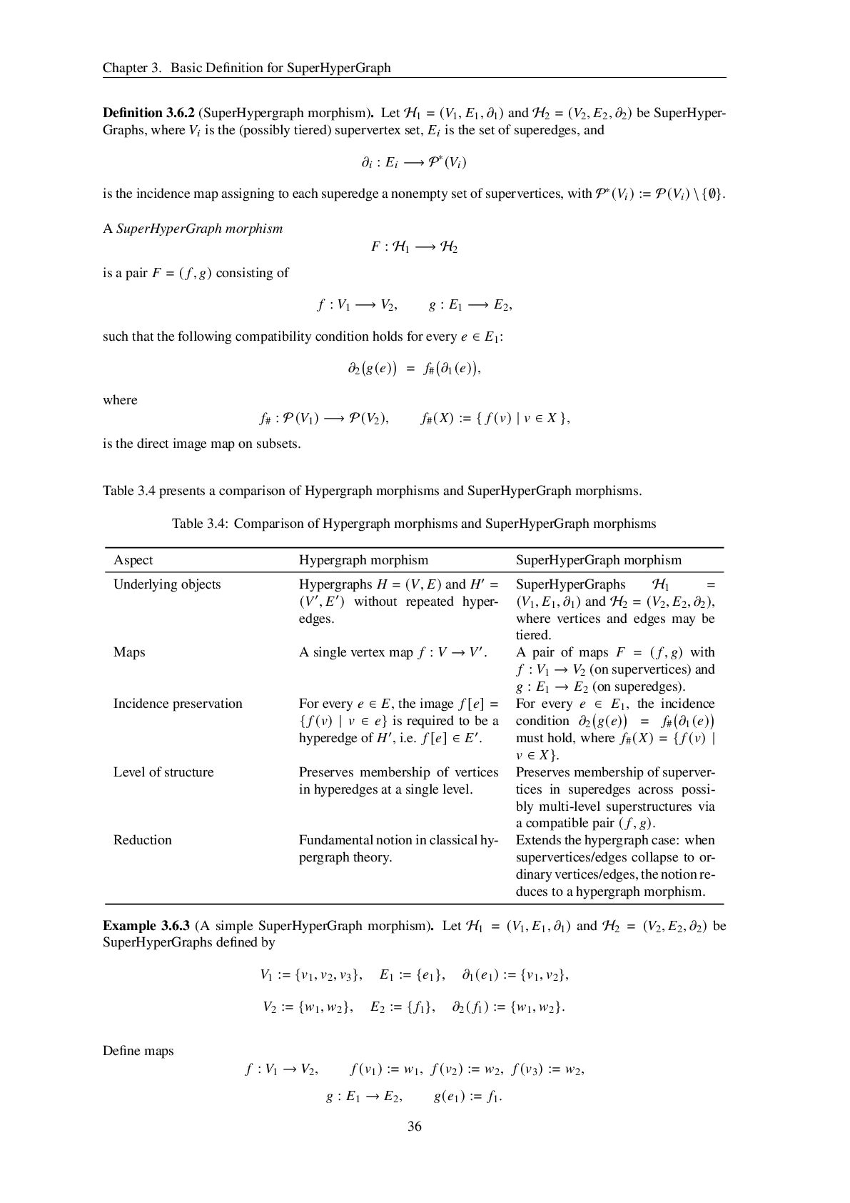
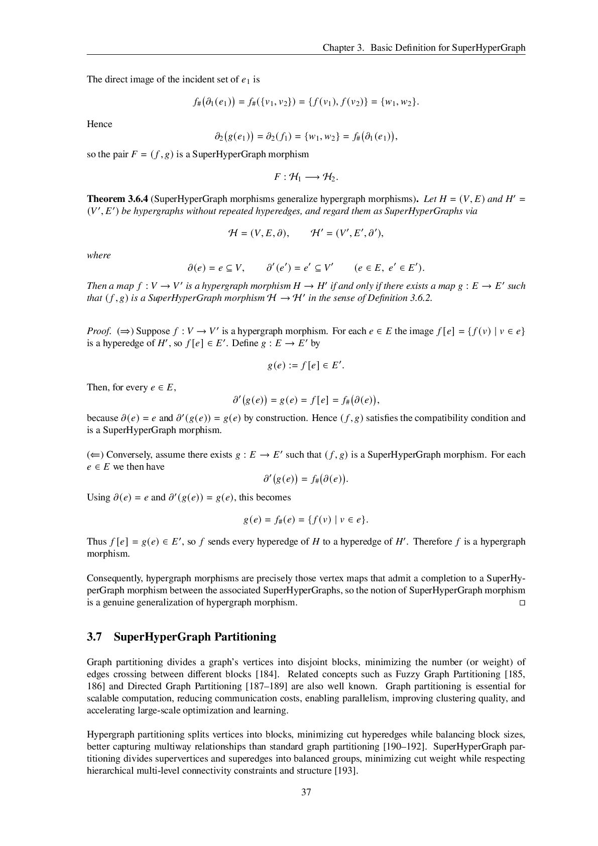
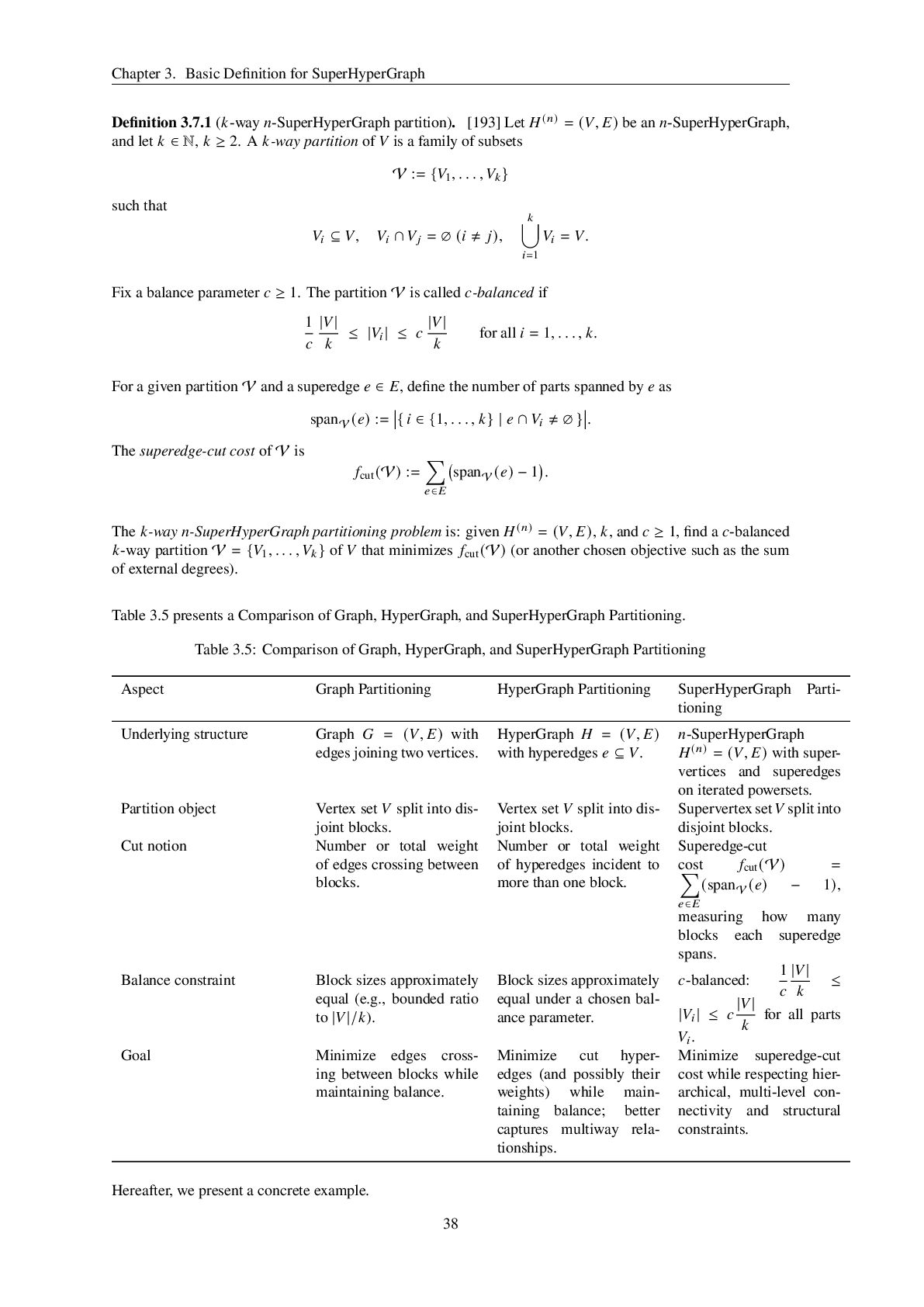
Bibliography [1032] Petros Maragos and Ronald W Schafer. Morphological systems
for multidimensional signal processing. Proceedings of the IEEE, 78(4):690–710, 2002. [1033] Tsuban Chen. The past, present, and future of image and multidimensional signal processing. IEEE Signal Processing Magazine, 15(2):21–58, 1998. [1034] Lital Dabush and Tirza Routtenberg. Verifying the smoothness of graph signals: A graph signal processing approach. IEEE Transactions on Signal Processing, 2024. [1035] Maria Alice Andrade Calazans, Felipe ABS Ferreira, Fernando AN Santos, Francisco Madeiro, and Juliano B Lima. Machine learning and graph signal processing applied to healthcare: A review. Bioengineering, 11(7):671, 2024. [1036] Muhammad Asaad Cheema, Muhammad Zohaib Sarwar, Vinay Chakravarthi Gogineni, Daniel Cantero, and Pierluigi Salvo Rossi. Computationally-efficient structural health monitoring using graph signal processing. IEEE Sensors Journal, 2024. [1037] Benjamin Ricaud, Pierre Borgnat, Nicolas Tremblay, Paulo Gonc ¸alves, and Pierre Vandergheynst. Fourier could be a data scientist: From graph fourier transform to signal processing on graphs. Comptes Rendus. Physique, 20(5):474–488, 2019. [1038] David I Shuman, Benjamin Ricaud, and Pierre Vandergheynst. A windowed graph fourier transform. In 2012 IEEE Statistical Signal Processing Workshop (SSP), pages 133–136. Ieee, 2012. [1039] Joao Domingos and Jos´ e MF Moura. Graph fourier transform: A stable approximation. IEEE Transactions on Signal Processing, 68:4422–4437, 2020. [1040] Gene Cheung, Enrico Magli, Yuichi Tanaka, and Michael K Ng. Graph spectral image processing. Proceedings of the IEEE, 106(5):907–930, 2018. [1041] Yuichi Tanaka. Graph spectral filtering. Graph Spectral Image Processing, page 3, 2021. [1042] Chen Gong, Tongliang Liu, Dacheng Tao, Keren Fu, Enmei Tu, and Jie Yang. Deformed graph laplacian for semisupervised learning. IEEE transactions on neural networks and learning systems, 26(10):2261–2274, 2015. [1043] Bo Jiang, Chris Ding, Bio Luo, and Jin Tang. Graph-laplacian pca: Closed-form solution and robustness. In Proceedings of the IEEE conference on computer vision and pattern recognition, pages 3492–3498, 2013. [1044] Sergio Barbarossa and Mikhail Tsitsvero. An introduction to hypergraph signal processing. In 2016 IEEE International Conference on Acoustics, Speech and Signal Processing (ICASSP), pages 6425–6429. IEEE, 2016. [1045] Xiaoying Song, Ke Wu, and Li Chai. Brain network analysis of schizophrenia patients based on hypergraph signal processing. IEEE Transactions on Image Processing, 32:4964–4976, 2023. [1046] Sang-Won Moon, Won-Sun Ruy, and Kwang-Phil Park. A study on fishing vessel energy system optimization using bond graphs. Journal of Marine Science and Engineering, 12(6):903, 2024. [1047] Peter Breedveld. Bond graphs. Encyclopedia of Life Support Systems, Modeling and Simulation, 2003. [1048] Mingfa Wang and Zhijun Jiang. The design and comparison of dc motor drive circuit in smart car competition. In 2009 IEEE International Conference on Intelligent Computing and Intelligent Systems, volume 2, pages 325–328. IEEE, 2009. [1049] Edward T Bullmore and Danielle S Bassett. Brain graphs: graphical models of the human brain connectome. Annual review of clinical psychology, 7(1):113–140, 2011. [1050] Qingbao Yu, Yuhui Du, Jiayu Chen, Jing Sui, T¨ ulay Adal¯ e, Godfrey D Pearlson, and Vince D Calhoun. Application of graph theory to assess static and dynamic brain connectivity: Approaches for building brain graphs. Proceedings of the IEEE, 106(5):886–906, 2018. [1051] Bhaskar Sen, Shu-Hsien Chu, and Keshab K Parhi. Ranking regions, edges and classifying tasks in functional brain graphs by sub-graph entropy. Scientific reports, 9(1):7628, 2019. [1052] Takaaki Fujita and Arkan A. Ghaib. Toward a unified theory of brain hypergraphs and symptom hypernetworks in medicine and neuroscience. Advances in Research, 26(3):522–565, 2025. [1053] Paul Axel-Lute. Legal citation form: Theory and practice. Law Libr. J., 75:148, 1982. [1054] Patti Ogden. Mastering the lawless science of our law: a story of legal citation indexes. Law Libr. J., 85:1, 1993. [1055] Ali Sadeghian, Laksshman Sundaram, D Wang, W Hamilton, Karl Branting, and Craig Pfeifer. Semantic edge labeling over legal citation graphs. In Proceedings of the workshop on legal text, document, and corpus analytics (LTDCA-2016), pages 70–75, 2016. [1056] Viktor Mayer-Schonberger and Yann Padova. Regime change? enabling big data through europe’s new data protection regulation. Colum. Sci. & Tech. L. Rev., 17:315, 2015. [1057] Edward S Dove. The eu general data protection regulation: implications for international scientific research in the digital era. Journal of Law, Medicine & Ethics, 46(4):1013–1030, 2018. [1058] Yogesh Ray and Pradeep Srivastava. Widespread aggradation in the mountainous catchment of the alaknanda–ganga river system: timescales and implications to hinterland–foreland relationships. Quaternary Science Reviews, 29(17-18):2238–2260, 2010. [1059] Rui Li, Xin Yuan, Mohsen Radfar, Peter Marendy, Wei Ni, Terrence J O’Brien, and Pablo M Casillas-Espinosa. Graph signal processing, graph neural network and graph learning on biological data: a systematic review. IEEE Reviews in Biomedical Engineering, 16:109–135, 2021. [1060] Fan Yang and Xingyue Huang. Theoretical insights into line graph transformation on graph learning. arXiv preprint arXiv:2410.16138, 2024. [1061] Sai Kiran Kadambari and Sundeep Prabhakar Chepuri. Product graph learning from multi-domain data with sparsity and rank constraints. IEEE Transactions on Signal Processing, 69:5665–5680, 2020. [1062] Cherukula Madhu and MS Sudhakar. An interpretable fuzzy graph learning for label propagation assisting data classification. IEEE Transactions on Fuzzy Systems, 32(3):1331–1345, 2023. 299

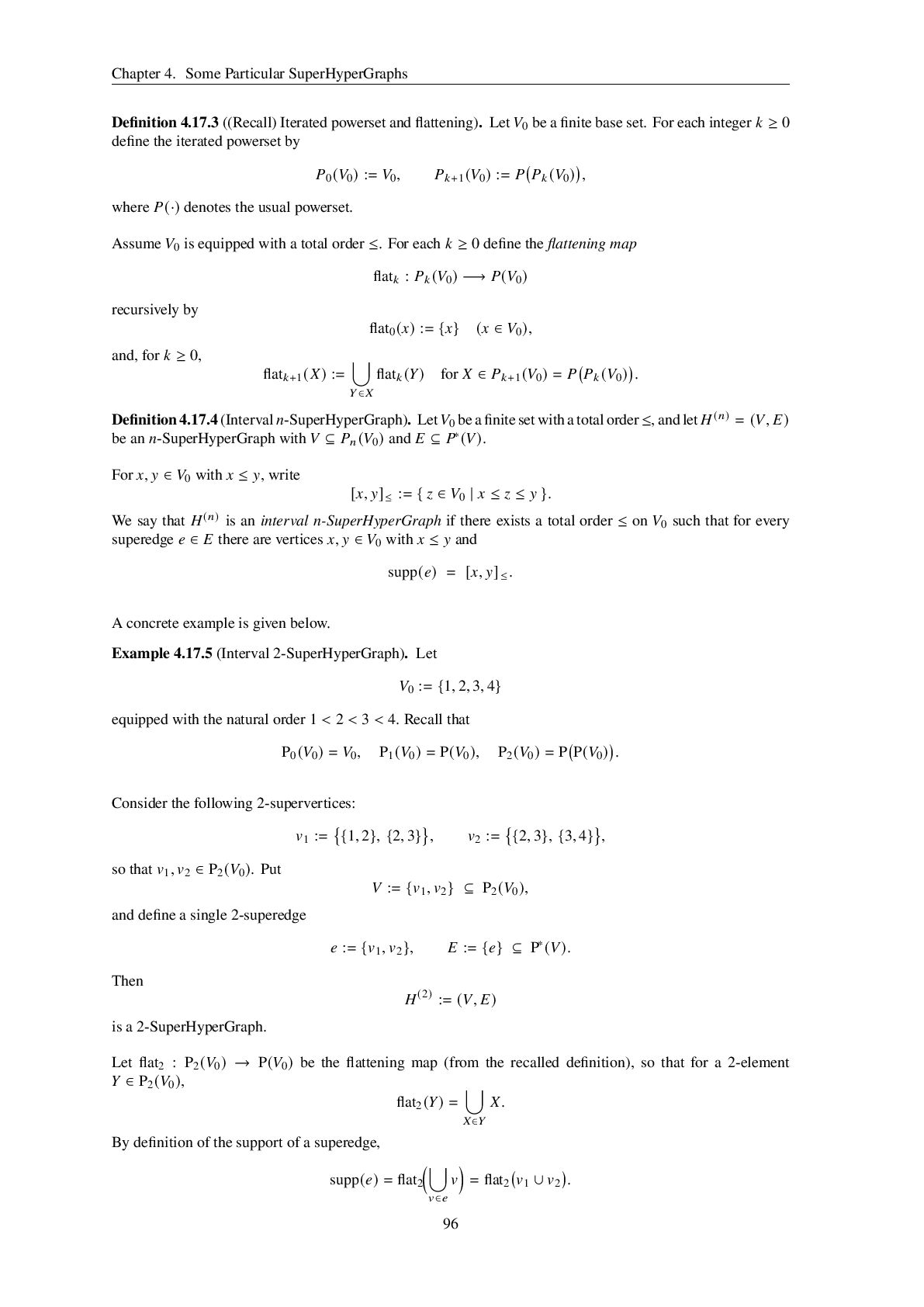
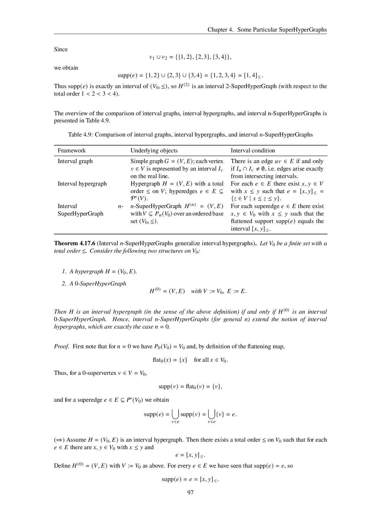
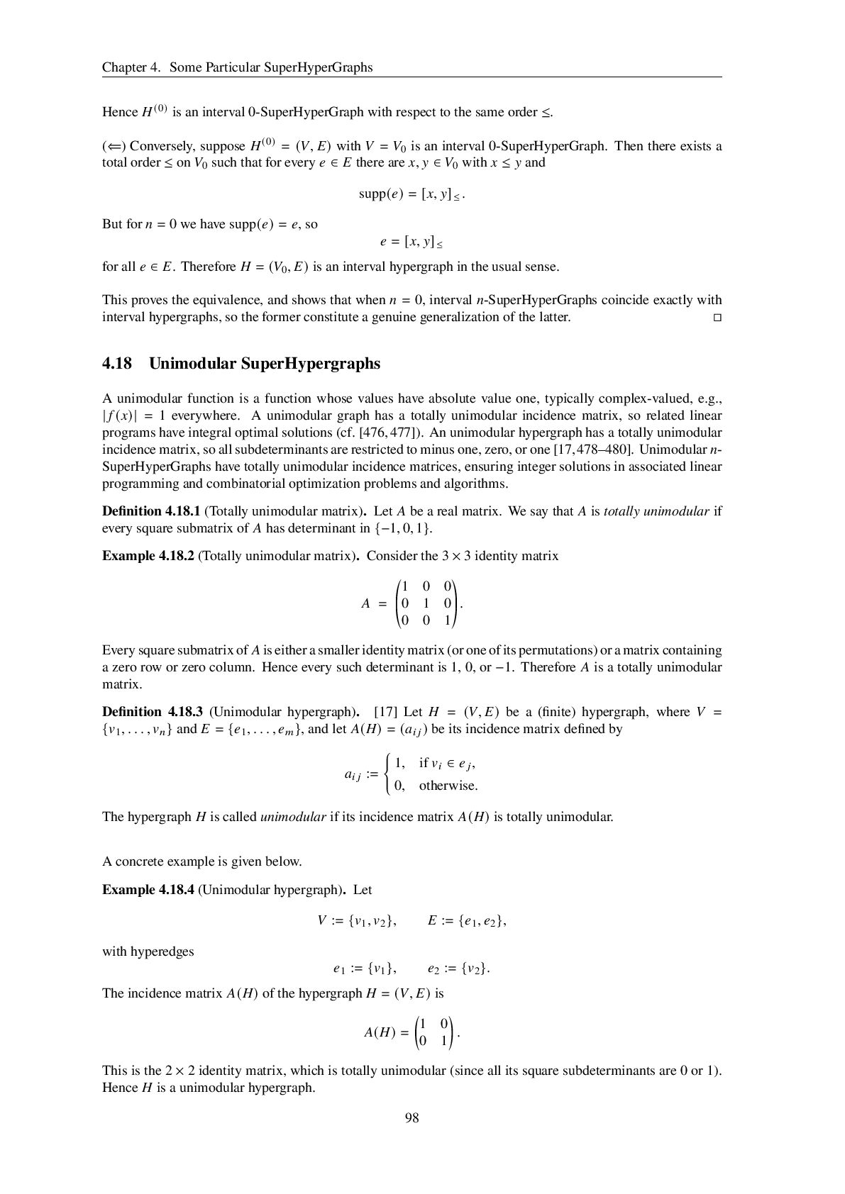
Bibliography [1063] Cherukula Madhu and MS Sudhakar. Dialectic feature-based fuzzy
graph learning for label propagation assisting text classification. IEEE Transactions on Fuzzy Systems, 32(10):5598–5612, 2024. [1064] Lingtong Min, Deyun Zhou, Xiaoyang Li, Qinyi Lv, and Yuanjie Zhi. Fuzzy graph learning regularized sparse filtering for visual domain adaptation. Applied Sciences, 11(10):4503, 2021. [1065] Fatemeh Kasraei and Arash Amini. Fast high-quality directed graph learning. In 2024 12th Iran Workshop on Communication and Information Theory (IWCIT), pages 1–6. IEEE, 2024. [1066] Kunpeng Zhang, Bin Jiang, Fuyang Chen, and Hui Yang. Directed-graph-learning-based diagnosis of multiple faults for high speed train with switched dynamics. IEEE Transactions on Cybernetics, 53(3):1712–1724, 2021. [1067] Hua Wang, Chris Ding, and Heng Huang. Directed graph learning via high-order co-linkage analysis. In Joint European Conference on Machine Learning and Knowledge Discovery in Databases, pages 451–466. Springer, 2010. [1068] Linh Nguyen Thi My and Tham Vo. Anti-symmetric molecular graph learning approach with residual adaptive network based fuzzy inference system for lethal dose forecasting problem. Journal of Computational Chemistry, 46(19):e70176, 2025. [1069] Yin Fang, Haihong Yang, Xiang Zhuang, Xin Shao, Xiaohui Fan, and Huajun Chen. Knowledge-aware contrastive molecular graph learning. arXiv preprint arXiv:2103.13047, 2021. [1070] Md Shamim Hussain, Mohammed J Zaki, and Dharmashankar Subramanian. Triplet interaction improves graph transformers: Accurate molecular graph learning with triplet graph transformers. arXiv preprint arXiv:2402.04538, 2024. [1071] Qiongjie Cui, Zongyuan Ding, and Fuhua Chen. Hybrid directed hypergraph learning and forecasting of skeleton-based human poses. Cyborg and Bionic Systems, 5:0093, 2024. [1072] Ruoxin Wang, Chi Fai Cheung, and Chunjin Wang. Heterogeneous hypergraph learning for analyzing surface defects in additive manufacturing process. Journal of Manufacturing Systems, 76:1–10, 2024. [1073] Ke Wu, Xiaoying Song, and Li Chai. Graph metrics based brain hypergraph learning in schizophrenia patients. 2022 China Automation Congress (CAC), pages 3251–3256, 2022. [1074] Shuting Jin, Yue Hong, Li Zeng, Yinghui Jiang, Yuan Lin, Leyi Wei, Zhuohang Yu, Xiangxiang Zeng, and Xiangrong Liu. A general hypergraph learning algorithm for drug multi-task predictions in micro-to-macro biomedical networks. PLOS Computational Biology, 19(11):e1011597, 2023. [1075] Jinming Xing, Ruilin Xing, Chang Xue, and Dongwen Luo. Enhancing link prediction with fuzzy graph attention networks and dynamic negative sampling. arXiv preprint arXiv:2411.07482, 2024. [1076] Weikang Zhou, Guangfu Ma, Nan Zhou, Xiaojun Liang, Cunnian Gao, Wenfeng Deng, Chunhua Yang, and Weihua Gui. Fgat: Industrial protocol states labeling with fuzzy graph attention network. Available at SSRN 5281432, 2025. [1077] Yi-Yang Feng, Hui Yu, Yue-Hua Feng, and Jian-Yu Shi. Directed graph attention networks for predicting asymmetric drug–drug interactions. Briefings in Bioinformatics, 23(3):bbac151, 2022. [1078] Jiafu Wu, Mufeng Yao, Dong Wu, Mingmin Chi, Baokun Wang, Ruofan Wu, Xin Fu, Changhua Meng, and Weiqiang Wang. Dedgat: Dual embedding of directed graph attention networks for detecting financial risk. arXiv preprint arXiv:2303.03933, 2023. [1079] Kaize Ding, Jianling Wang, Jundong Li, Dingcheng Li, and Huan Liu. Be more with less: Hypergraph attention networks for inductive text classification. arXiv preprint arXiv:2011.00387, 2020. [1080] Jianling Wang, Kaize Ding, Ziwei Zhu, and James Caverlee. Session-based recommendation with hypergraph attention networks. In Proceedings of the 2021 SIAM international conference on data mining (SDM), pages 82–90. SIAM, 2021. [1081] Eun-Sol Kim, Woo Young Kang, Kyoung-Woon On, Yu-Jung Heo, and Byoung-Tak Zhang. Hypergraph attention networks for multimodal learning. In Proceedings of the IEEE/CVF conference on computer vision and pattern recognition, pages 14581–14590, 2020. [1082] Chaofan Chen, Zelei Cheng, Zuotian Li, and Manyi Wang. Hypergraph attention networks. In 2020 IEEE 19th International Conference on Trust, Security and Privacy in Computing and Communications (TrustCom), pages 1560–1565. IEEE, 2020. [1083] Takaaki Fujita and Arif Mehmood. Superhypergraph attention networks. Neutrosophic Computing and Machine Learning, 40(1):10–27, 2025. [1084] Takaaki Fujita. Hypergraph- and superhypergraph-based models for patient care, disease transmission, and healthcare collaboration networks (with an exploration of (𝑚, 𝑛)-superhypergraphs), 2024. [1085] Maissam Jdid, Florentin Smarandache, and Takaaki Fujita. A linear mathematical model of the vocational training problem in a company using neutrosophic logic, hyperfunctions, and superhyperfunction. Neutrosophic Sets and Systems, 87:1–11, 2025. [1086] Derun Cai, Moxian Song, Chenxi Sun, Baofeng Zhang, Shenda Hong, and Hongyan Li. Hypergraph structure learning for hypergraph neural networks. In IJCAI, pages 1923–1929, 2022. [1087] Daniele Pretolani. Finding hypernetworks in directed hypergraphs. European Journal of Operational Research, 230(2):226–230, 2013. [1088] Aur´ elien Ducournau and Alain Bretto. Random walks in directed hypergraphs and application to semi-supervised image segmentation. Computer Vision and Image Understanding, 120:91–102, 2014. [1089] Maurice Heins. Complex Function Theory: Complex Function Theory, volume 28. Academic Press, 1968. [1090] David Gems. The hyperfunction theory: an emerging paradigm for the biology of aging. Ageing research reviews, 74:101557, 2022. [1091] Takaaki Fujita. Hyperfunction and superhyperfunction in machine learning: Loss, activation, cost, objective, scoring, probability density, and radial basis. Authorea Preprints, 2025. [1092] John R Durbin. Modern algebra: An introduction. John Wiley & Sons, 2008. [1093] Alekseui Ivanovich Kostrikin and Roberto Anibal Sala. Introduction to algebra, volume 8. Springer, 1982. 300

Bibliography [1094] Ivo G Rosenberg. An algebraic approach to hyperalgebras.
In Proceedings of 26th IEEE International Symposium on Multiple- Valued Logic (ISMVL’96), pages 203–207. IEEE, 1996. [1095] Kostaq Hila, Serkan Onar, Bayram Ali Ersoy, and Bijan Davvaz. On generalized intuitionistic fuzzy subhyperalgebras of boolean hyperalgebras. Journal of Inequalities and Applications, 2013:1–15, 2013. [1096] Takaaki Fujita and Florentin Smarandache. Neutrosophic TwoFold SuperhyperAlgebra and Anti SuperhyperAlgebra. Infinite Study, 2025. [1097] Ajoy Kanti Das, Suman Patra, Takaaki Fujita, and Suman Das. Advanced structures in superhyper algebra: Monoids and ideals. Boletim da Sociedade Paranaense de Matematica, 43:1–17, 2025. [1098] Florentin Smarandache. Introduction to the n-SuperHyperGraph-the most general form of graph today. Infinite Study, 2022. [1099] Dimitrios Tsiotas and Serafeim Polyzos. The topology of urban road networks and its role to urban mobility. Transportation research procedia, 24:482–490, 2017. [1100] K Reji Kumar and SA Naisal. Interior exterior and boundary of fuzzy soft multi topology in decision making. In 2016 International Conference on Control, Instrumentation, Communication and Computational Technologies (ICCICCT), pages 147–152. IEEE, 2016. [1101] Florentin Smarandache. New types of topologies and neutrosophic topologies (improved version). Neutrosophic Sets and Systems, 57(1):14, 2023. [1102] P Gnanachandra, C Arunthathi, and S Jafari. Mathematical foundations and structural analysis of superhyper topology generated from binary relations. SuperHyperTopologies and SuperHyperStructures with their Applications, page 13, 2025. [1103] Takaaki Fujita. Plithogenic superhypertopology and superhyperneutrosophic superhypertopology. SuperHyperTopologies and SuperHyperStructures with their Applications, page 142, 2025. [1104] Dietrich Burde. Group theory. Computers, Rigidity, and Moduli, 2019. [1105] Bahman Zohuri, Seyed Kamal Mousavi Balgehshiri, and Mohammad Amin Imani. Harmony in complexity exploring the synergy of fuzzy logic, group theory, and artificial intelligence. Nov Joun of Appl Sci Res, 1 (2), 01, 7, 2024. [1106] Bijan Davvaz. Semihypergroup theory. Academic Press, 2016. [1107] Ganeshsree Selvachandran and Abdul Razak Salleh. Soft hypergroups and soft hypergroup homomorphism. In AIP Conference Proceedings. American Institute of Physics, 2013. [1108] Takaaki Fujita. Superhypermagma, lie superhypergroup, quotient superhypergroups, and reduced superhypergroups. International Journal of Topology, 2(3):10, 2025. [1109] Martin A. Dufwenberg. Game theory. Wiley interdisciplinary reviews. Cognitive science, 2 2:167–173, 2011. [1110] Martin J. Osborne and Ariel Rubinstein. A Course in Game Theory. MIT press, 1995. [1111] Takaaki Fujita. Rethinking strategic perception: Foundations and advancements in hypergame theory and superhypergame theory. Prospects for Applied Mathematics and Data Analysis, 4(2):01–14, 2024. [1112] Jos´ e Unpingco. Python for probability, statistics, and machine learning, volume 1. Springer, 2016. [1113] Jochen Kruppa, Yufeng Liu, G´ erard Biau, Michael Kohler, Inke R K¨ onig, James D Malley, and Andreas Ziegler. Probability estimation with machine learning methods for dichotomous and multicategory outcome: theory. Biometrical Journal, 56(4):534– 563, 2014. [1114] Takaaki Fujita. An introduction and reexamination of hyperprobability and superhyperprobability: Comprehensive overview. Asian Journal of Probability and Statistics, 27(5):82–109, 2025. [1115] Meir Feder and Neri Merhav. Relations between entropy and error probability. IEEE Transactions on Information theory, 40(1):259–266, 2002. [1116] Jean U Thoma. Bond graphs for thermal energy transport and entropy flow. Journal of the Franklin Institute, 292(2):109–120, 1971. [1117] Takaaki Fujita. Entropy reimagined: Theoretical foundations of hyperentropy and superhyperentropy with real-world and engineering applications. Spectrum of Engineering and Management Sciences, 3(1):262–286, 2025. [1118] Edward H Sussenguth. A graph-theoretic algorithm for matching chemical structures. Journal of Chemical Documentation, 5(1):36–43, 1965. [1119] Sourav Mondal, Nilanjan De, and Anita Pal. Topological indices of some chemical structures applied for the treatment of covid-19 patients. Polycyclic Aromatic Compounds, 42(4):1220–1234, 2022. [1120] M Al Tahan and Bijan Davvaz. Weak chemical hyperstructures associated to electrochemical cells. Iranian Journal of Mathematical Chemistry, 9(1):65–75, 2018. [1121] Madeleine Al-Tahan and Bijan Davvaz. Chemical hyperstructures for elements with four oxidation states. Iranian Journal of Mathematical Chemistry, 13(2):85–97, 2022. [1122] Sang-Cho Chung. Chemical hyperstructures for ozone depletion. Journal of the Chungcheong Mathematical Society, 32(4):491– 508, 2019. [1123] Takaaki Fujita. Chemical hyperstructures, superhyperstructures, and shv-structures: Toward a generalized framework for hierarchical chemical modeling, 2025. [1124] BF Melnikov. The complete finite automaton. International Journal of Open Information Technologies, 5(10):9–17, 2017. [1125] Pierre Fraigniaud, David Ilcinkas, Guy Peer, Andrzej Pelc, and David Peleg. Graph exploration by a finite automaton. Theoretical Computer Science, 345(2-3):331–344, 2005. [1126] Takaaki Fujita and Florentin Smarandache. Uncertain automata and uncertain graph grammar. Neutrosophic Sets and Systems, 74:128–191, 2024. 301

Bibliography [1127] Takaaki Fujita. Powerset-theoretic foundations for hyperautomata and superhyperautomata.
Systemic Analytics, 3(3):222–231, 2025. [1128] Lotfi A Zadeh. A computational approach to fuzzy quantifiers in natural languages. In Computational linguistics, pages 149–184. Elsevier, 1983. [1129] Harry M Hersh and Alfonso Caramazza. A fuzzy set approach to modifiers and vagueness in natural language. Journal of Experimental Psychology: General, 105(3):254, 1976. [1130] Takaaki Fujita. Theoretical interpretations of large uncertain and hyper language models: Advancing natural uncertain and hyper language processing. Advancing Uncertain Combinatorics through Graphization, Hyperization, and Uncertainization: Fuzzy, Neutrosophic, Soft, Rough, and Beyond, page 245, 2025. [1131] Takaaki Fujita. From natural language to superhyperlanguage: A foundational survey of hierarchical language frameworks, 2025. [1132] Spiro Karigiannis. Introduction to geometry. In Lectures and Surveys on G2-manifolds and related topics, pages 3–50. Springer, 2020. [1133] Duncan MY Sommerville. Introduction to the Geometry of N Dimensions. Courier Dover Publications, 2020. [1134] Takaaki Fujita. A formal framework for fuzzy hypergeometry: Extending fuzzy geometry through hyperstructural methods. International Journal of Computer Discovered Mathematics (IJCDM), 10:500–511, 2025. [1135] Takaaki Fujita. A comprehensive review of hypergeometry and superhypergeometry. International Journal of Computer Discovered Mathematics (IJCDM), 10:489–499, 2025. [1136] Takaaki Fujita. Antihypergeometry, neutrohypergeometry, and superhypergeometry. Advancing Uncertain Combinatorics through Graphization, Hyperization, and Uncertainization: Fuzzy, Neutrosophic, Soft, Rough, and Beyond, page 568, 2025. [1137] Takaaki Fujita. Metastructure, meta-hyperstructure, and meta-superhyper structure. Journal of Computers and Applications, 1(1):1–22, 2025. [1138] Claude Bernard. An introduction to the study of experimental medicine, volume 400. Courier Corporation, 1957. [1139] Yu. F. Zin’kovskii and B. M. Uvarov. Hyper-randomness of algorithms for simulation of current radio electronic equipment. Radioelectronics and Communications Systems, 54:147–154, 2011. [1140] Takaaki Fujita. A theoretical exploration of hyperconcepts: Hyperfunctions, hyperrandomness, hyperdecision-making, and beyond (including a survey of hyperstructures). Advancing Uncertain Combinatorics through Graphization, Hyperization, and Uncertainization: Fuzzy, Neutrosophic, Soft, Rough, and Beyond, page 111, 2025. [1141] M. Kaur and A. Singh. Approach to multi-criteria decision-making in a neutrosophic picture hyper-soft set environment using generalized neutrosophic topsis. Neutrosophic Sets and Systems, 67(1):5, 2024. [1142] Alex Gabriel Lara Jacome, Elizabeth Mayorga Aldaz, Miguel Ramos Argilagos, and Darvin Manuel Ram´ ırez Guerra. Neutrosophic perspectives in healthcare decision-making: Navigating complexity with ethics, information, and collaboration. Neutrosophic Sets and Systems, 62(1):15, 2023. [1143] Farnaz Sabahi and Mohammad Reza Akbarzadeh-Totonchi. Introducing validity in fuzzy probability for judicial decision-making. Int. J. Approx. Reason., 55:1383–1403, 2014. [1144] Takaaki Fujita. Some types of hyperdecision-making and superhyperdecision-making. Advancing Uncertain Combinatorics through Graphization, Hyperization, and Uncertainization: Fuzzy, Neutrosophic, Soft, Rough, and Beyond, page 221, 2025. [1145] Steve Awodey. Category theory, volume 52. OUP Oxford, 2010. [1146] Paolo Perrone. Notes on category theory with examples from basic mathematics. arXiv preprint arXiv:1912.10642, 2019. [1147] Geoffrey Hellman. Does category theory provide a framework for mathematical structuralism? Philosophia Mathematica, 11(2):129–157, 2003. [1148] Takaaki Fujita. A brief study on superhypercategories. Advancing Uncertain Combinatorics through Graphization, Hyperization, and Uncertainization: Fuzzy, Neutrosophic, Soft, Rough, and Beyond, page 360, 2025. [1149] Stanis law Saks. Theory of the integral, 1937. [1150] AB Prudnikov. Integrals and series. Routledge, 2018. [1151] Takaaki Fujita. Short note of superhyperstructures of partitions, integrals, and spaces. Advancing Uncertain Combinatorics through Graphization, Hyperization, and Uncertainization: Fuzzy, Neutrosophic, Soft, Rough, and Beyond, page 384, 2025. [1152] Hongxing Li and Vincent C Yen. Fuzzy sets and fuzzy decision-making. CRC press, 1995. [1153] Jayanta Ghosh and Tapas Kumar Samanta. Hyperfuzzy sets and hyperfuzzy group. Int. J. Adv. Sci. Technol, 41:27–37, 2012. [1154] Seok-Zun Song, Seon Jeong Kim, and Young Bae Jun. Hyperfuzzy ideals in bck/bci-algebras. Mathematics, 5(4):81, 2017. [1155] Z Nazari and B Mosapour. The entropy of hyperfuzzy sets. Journal of Dynamical Systems and Geometric Theories, 16(2):173–185, 2018. [1156] Takaaki Fujita. Weak hyperfuzzy set and weak superhyperfuzzy set. Computational Methods, 2(1):11–26, 2025. [1157] Takaaki Fujita and Florentin Smarandache. Examples of fuzzy sets, hyperfuzzy sets, and superhyperfuzzy sets in climate change and the proposal of several new concepts. Climate Change Reports, 2:1–18, 2025. [1158] Florentin Smarandache. Hyperuncertain, superuncertain, and superhyperuncertain sets/logics/probabilities/statistics. Infinite Study, 2017. [1159] Takaaki Fujita. Hyperweighted and superhyperweighted multigraphs: Foundations and real-world applications. Soft Computing Fusion With Applications, 2025. [1160] An Lu and Wilfred Ng. Vague sets or intuitionistic fuzzy sets for handling vague data: which one is better? In International conference on conceptual modeling, pages 401–416. Springer, 2005. 302

Bibliography [1161] W-L Gau and Daniel J Buehrer. Vague sets.
IEEE transactions on systems, man, and cybernetics, 23(2):610–614, 1993. [1162] Takaaki Fujita. Advancing Uncertain Combinatorics through Graphization, Hyperization, and Uncertainization: Fuzzy, Neutro- sophic, Soft, Rough, and Beyond. Biblio Publishing, 2025. [1163] Suman Das, Rakhal Das, and Surapati Pramanik. Single valued pentapartitioned neutrosophic graphs. Neutrosophic Sets and Systems, 50(1):225–238, 2022. [1164] Takaaki Fujita and Florentin Smarandache. Hyperneutrosophic set and forest hyperneutrosophic set with practical applications in agriculture. Optimization in Agriculture, 2:10–21, 2025. [1165] Takaaki Fujita and Florentin Smarandache. Some types of hyperneutrosophic set (5): Support, paraconsistent, faillibilist, and others. Advancing Uncertain Combinatorics through Graphization, Hyperization, and Uncertainization: Fuzzy, Neutrosophic, Soft, Rough, and Beyond, 2025. [1166] Takaaki Fujita and Florentin Smarandache. Hierarchical uncertainty modeling via (m, n)-superhyperuncertainand (h, k)-ary (m, n)-superhyperuncertain sets: Unified extensions of fuzzy, neutrosophic, soft, rough, and plithogenic set theories. European Journal of Pure and Applied Mathematics, 18(4):6834–6834, 2025. [1167] Florentin Smarandache. Plithogeny, plithogenic set, logic, probability, and statistics. Infinite Study, 2017. [1168] Takaaki Fujita. Hyperplithogenic cubic set and superhyperplithogenic cubic set. Advancing Uncertain Combinatorics through Graphization, Hyperization, and Uncertainization: Fuzzy, Neutrosophic, Soft, Rough, and Beyond, page 79, 2025. [1169] Takaaki Fujita and Florentin Smarandache. Exploring Concepts of HyperFuzzy, HyperNeutrosophic, and HyperPlithogenic Sets (I). Infinite Study, 2025. [1170] Takaaki Fujita. Symbolic hyperplithogenic set. Advancing Uncertain Combinatorics through Graphization, Hyperization, and Uncertainization: Fuzzy, Neutrosophic, Soft, Rough, and Beyond, page 130, 2025. [1171] Said Broumi, Florentin Smarandache, and Mamoni Dhar. Rough neutrosophic sets. Infinite Study, 32:493–502, 2014. [1172] Takaaki Fujita and Florentin Smarandache. A concise introduction to hyperfuzzy, hyperneutrosophic, hyperplithogenic, hypersoft, and hyperrough sets with practical examples. Neutrosophic Sets and Systems, 80:609–631, 2025. [1173] T. Fujita. Note of indetermrough set and indetermhyperrough set. Information Sciences with Applications, 7:1–14, 2025. [1174] Takaaki Fujita and Arif Mehmood. Hyperrough number and superhyperrough number with applications. Applied Research Advances, pages 1–16, 2026. [1175] Florentin Smarandache. Extension of soft set to hypersoft set, and then to plithogenic hypersoft set. Neutrosophic sets and systems, 22(1):168–170, 2018. [1176] Mona Mohamed, Ahmed M AbdelMouty, Khalid Mohamed, and Florentin Smarandache. Superhypersoft-driven evaluation of smart transportation in centroidous-moosra: Real-world insights for the uav era. Neutrosophic Sets and Systems, 78:149–163, 2025. [1177] Abdullah Ali Salamai. A superhypersoft framework for comprehensive risk assessment in energy projects. Neutrosophic Sets and Systems, 77:614–624, 2025. [1178] Florentin Smarandache. Foundation of the superhypersoft set and the fuzzy extension superhypersoft set: A new vision. Neutro- sophic Systems with Applications, 11:48–51, 2023. [1179] Muhammad Kamran, Nadeem Salamat, and Muhammad Shazib Hameed. Sine trigonometric aggregation operators with single- valued neutrosophic z-numbers: Application in business site selection. Neutrosophic Sets and Systems, 63(1):18, 2024. [1180] Hui Li, Xuefei Liao, Zhen Li, Lei Pan, Meng Yuan, and Ke Qin. The operational laws of symmetric triangular z-numbers. Mathematics, 12(10):1443, 2024. [1181] Lotfi A Zadeh. A note on z-numbers. Information sciences, 181(14):2923–2932, 2011. [1182] Takaaki Fujita. Concise note of z-number, hyper z-number, and superhyper z-number. Advancing Uncertain Combinatorics through Graphization, Hyperization, and Uncertainization: Fuzzy, Neutrosophic, Soft, Rough, and Beyond, 6(25):352, 2025. [1183] Somen Debnath. Fuzzy quadripartitioned neutrosophic soft matrix theory and its decision-making approach. Journal of Compu- tational and Cognitive Engineering, 1(2):88–93, 2022. [1184] Antonia Maria Tulino and Sergio Verd´ u. Random matrix theory and wireless communications. Found. Trends Commun. Inf. Theory, 1, 2004. [1185] C. W. J. Beenakker. Random-matrix theory of quantum transport. Reviews of Modern Physics, 69:731–808, 1996. [1186] Maedeh Motameni, Reza Ameri, and R. Sadeghi. Hypermatrix based on krasner hypervector spaces. Ratio Mathematica, 25(1), 2013. [1187] Takaaki Fujita. Hypermatrix, superhypermatrix, multimatrix, iterative multimatrix, metamatrix, and iterated metamatrix, 2025. [1188] Richard M. Satur and Zhi qiang Liu. A contextual fuzzy cognitive map framework for geographic information systems. IEEE Trans. Fuzzy Syst., 7:481–494, 1999. [1189] Zhi qiang Liu and Richard M. Satur. Contextual fuzzy cognitive map for decision support in geographic information systems. IEEE Trans. Fuzzy Syst., 7:495–507, 1999. [1190] Suman Rao. Red teaming military intelligence-a new approach based on neutrosophic cognitive mapping. In 2010 IEEE International Conference on Intelligent Systems and Knowledge Engineering, pages 622–627. IEEE, 2010. [1191] Zhou Feng, Bo Yao, and Chung-Kuan Cheng. Floorplan representation in vlsi. In Handbook of Data Structures and Applications, pages 833–855. Chapman and Hall/CRC, 2018. [1192] Carsten F Ball, Peter V Kraus, and Dieter A Mlynski. Fuzzy partitioning applied to vlsi-floorplanning and placement. In Proceedings of IEEE International Symposium on Circuits and Systems-ISCAS’94, volume 1, pages 177–180. IEEE, 1994. 303

Bibliography [1193] Takaaki Fujita. Superhypercode and superhyperfloorplan. Advancing Uncertain Combinatorics
through Graphization, Hyperiza- tion, and Uncertainization: Fuzzy, Neutrosophic, Soft, Rough, and Beyond, page 326, 2025. [1194] Robert Wisbauer. Foundations of module and ring theory. Routledge, 2018. [1195] Bo Stenstrom. Rings of quotients: an introduction to methods of ring theory, volume 217. Springer Science & Business Media, 2012. [1196] Fakhry Asad Agusfrianto, Saba Al-Kaseasbeh, Mariam Hariri, and Yudi Mahatma. On neutrohyperrings and neutroorderedhy- perrings. Neutrosophic Sets and Systems, 77:1–19, 2025. [1197] Marc Krasner et al. A class of hyperrings and hyperfields. International Journal of Mathematics and Mathematical Sciences, 6(2):307–311, 1983. [1198] Florentin Smarandache. Foundation of superhyperstructure & neutrosophic superhyperstructure. Neutrosophic Sets and Systems, 63(1):21, 2024. [1199] Philip Schwed. Topics in field theory., 1948. [1200] THOMAS Vougiouklis. The fundamental relation in hyperrings. the general hyperfield. In Proc. Fourth Int. Congress on Algebraic Hyperstructures and Applications (AHA 1990), World Scientific, pages 203–211. World Scientific, 1991. [1201] Oleg Ya. Viro. Hyperfields for tropical geometry i. hyperfields and dequantization. arXiv: Algebraic Geometry, 2010. [1202] Stanis law Zukowski. Introduction to lattice theory. Formalized Mathematics, 1(1):215–222, 1990. [1203] Pengfei He and Xiaolong Xin. Fuzzy hyperlattices. Computers & Mathematics with Applications, 62(12):4682–4690, 2011. [1204] Pengfei He, Xiaolong Xin, and Jianming Zhan. On rough hyperideals in hyperlattices. Journal of Applied Mathematics, 2013(1):915217, 2013. [1205] Bijan Davvaz, Wieslaw A Dudek, and Thomas Vougiouklis. A generalization of n-ary algebraic systems. Communications in Algebra, 37(4):1248–1263, 2009. [1206] Maria Santilli Ruggero and Thomas Vougiouklis. Hyperstructures in lie-santilli admissibility and iso-theories. Ratio Mathematica, 33:151, 2017. [1207] Madeleine Al-Tahan, Bijan Davvaz, Florentin Smarandache, and Osman Anis. On some neutrohyperstructures. Symmetry, 13(4):535, 2021. [1208] Fakhry Asad Agusfrianto, Madeleine Al Tahan, and Yudi Mahatma. An introduction to neutrohyperstructures on some chemical reactions. In NeutroGeometry, NeutroAlgebra, and SuperHyperAlgebra in Today’s World, pages 81–96. IGI Global, 2023. [1209] Fakhry Asad Agusfrianto, Madeleine Al-Tahan, Mariam Hariri, and Yudi Mahatma. Examples of neutrohyperstructures on biological inheritance. Neutrosophic Sets and Systems, 60:583–592, 2023. [1210] Alexander W. Kocurek. The logic of hyperlogic. part a: Foundations. The Review of Symbolic Logic, 17:244 – 271, 2022. [1211] Mark Burgin. Integrating random properties and the concept of probability. Integration, 3(2):137–155, 2012. [1212] Ferdinand ¨ Osterreicher and Igor Vajda. A new class of metric divergences on probability spaces and its applicability in statistics. Annals of the Institute of Statistical Mathematics, 55:639–653, 2003. [1213] Jian Tang, Xinyang Feng, Bijan Davvaz, and Xiangyun Xie. A further study on ordered regular equivalence relations in ordered semihypergroups. Open Mathematics, 16:168 – 184, 2018. [1214] Muhammad Farooq, Asghar Khan, and Bijan Davvaz. Characterizations of ordered semihypergroups by the properties of their intersectional-soft generalized bi-hyperideals. Soft Computing, 22:3001–3010, 2018. [1215] Marc Krasner. A class of hyperrings and hyperfields. International Journal of Mathematics and Mathematical Sciences, 6:307–311, 1983. [1216] Achilles Dramalidis and Thomas Vougiouklis. Fuzzy hv-substructures in a two dimensional euclidean vector space. Iranian Journal of Fuzzy Systems, 6(4):1–9, 2009. [1217] M Scafati Tallini. Hypervector spaces. In Proceeding of the 4th International Congress in Algebraic Hyperstructures and Applications, pages 167–174, 1991. [1218] Hans-Jurgen Bandelt and Victor Chepoi. Metric graph theory and geometry: a survey. Contemporary Mathematics, 453:49–86, 2008. [1219] Tomaz Pisanski and Milan Randic. Bridges between geometry and graph theory. In Catherine A. Gorini, editor, Geometry at Work, volume 53 of MAA Notes, pages 174–194. Cambridge University Press, 2000. [1220] FS Al-Anzi. Efficient cellular automata algorithms for planar graph and vlsi layout homotopic compaction. International Journal of Computing and Information Sciences, 1(1):1–17, 2003. [1221] John E Hopcroft and Jeffrey D Ullman. Formal languages and their relation to automata. Addison-Wesley Longman Publishing Co., Inc., 1969. [1222] H¨ useyin Kamacı. Linguistic single-valued neutrosophic soft sets with applications in game theory. International Journal of Intelligent Systems, 36(8):3917–3960, 2021. [1223] Nicholas Kovach, Alan S. Gibson, and Gary B. Lamont. Hypergame theory: A model for conflict, misperception, and deception. Game Theory, 2015, 2015. [1224] Akbar Rezaei, Florentin Smarandache, and S. Mirvakili. Applications of (neutro/anti)sophications to semihypergroups. Journal of Mathematics, 2021. [1225] Souzana Vougioukli. Helix-hyperoperations on lie-santilli admissibility. Algebras Groups and Geometries, 2023. [1226] Bijan Davvaz and Thomas Vougiouklis. Walk Through Weak Hyperstructures, A: Hv-structures. World Scientific, 2018. 304

Bibliography [1227] Piergiulio Corsini and Violeta Leoreanu. Applications of hyperstructure
theory, volume 5. Springer Science & Business Media, 2013. [1228] Takaaki Fujita. Toward a formal framework of physical superhyperstructures: Multi-layered extensions of hyperstructures in physics. Neutrosophic Optimization and Intelligent Systems, 8:1–18, 2025. [1229] Florentin Smarandache. Superhyperstructure & neutrosophic superhyperstructure, 2024. Accessed: 2024-12-01. [1230] Abdullah Kargın and Memet S ¸ahin. Superhyper groups and neutro–superhyper groups. 2023 Neutrosophic SuperHyperAlgebra And New Types of Topologies, 25, 2023. [1231] Florentin Smarandache. History of superhyperalgebra and neutrosophic superhyperalgebra (revisited again). Neutrosophic Algebraic Structures and Their Applications, page 10, 2022. [1232] Eduardo Luciano Hernandez Ramos, Luis Ramiro Ayala Ayala, and Kevin Alexander Samaniego Macas. Study of factors that influence a victim’s refusal to testify for sexual reasons due to external influence using plithogenic 𝑛-superhypergraphs. Operational Research Journal, 46(2):328–337, 2025. [1233] Sirus Jahanpanah and Roohallah Daneshpayeh. On derived superhyper be-algebras. Neutrosophic Sets and Systems, 57(1):21, 2023. [1234] F. Smarandache. Introduction to superhyperalgebra and neutrosophic superhyperalgebra. Journal of Algebraic Hyperstructures and Logical Algebras, 2022. [1235] N Vinoth Kumar and G Geetha Ramani. Product intuitionistic fuzzy graph. International Journal of Computer Applications, 28(1):31–33, 2011. [1236] Muhammad Akram, Bijan Davvaz, and Feng Feng. Intuitionistic fuzzy soft k-algebras. Mathematics in Computer Science, 7:353–365, 2013. [1237] Zengtai Gong and Junhu Wang. Hesitant fuzzy graphs, hesitant fuzzy hypergraphs and fuzzy graph decisions. Journal of Intelligent & Fuzzy Systems, 40(1):865–875, 2021. [1238] Muhammad Akram, MG Karunambigai, K Palanivel, and S Sivasankar. Balanced bipolar fuzzy graphs. Journal of advanced research in pure mathematics, 6(4):58–71, 2014. [1239] Said Broumi, Assia Bakali, Mohamed Talea, Florentin Smarandache, and Kifayat Ullah. Bipolar neutrosophic minimum spanning tree. Infinite Study, 127, 2018. [1240] WB Vasantha Kandasamy, K Ilanthenral, and Florentin Smarandache. Plithogenic Graphs. Infinite Study, 2020. [1241] Igor E Zverovich. Multi-intersection graphs. Discrete Mathematics, 218(1-3):245–251, 2000. [1242] Wayne D. Blizard et al. Multiset theory. Notre Dame Journal of formal logic, 30(1):36–66, 1989. [1243] Petr Chmel and V´ ıt Jel´ ınek. String graphs with precise number of intersections. In International Symposium on Graph Drawing and Network Visualization, pages 78–92. Springer, 2023. [1244] J´ anos Pach, Bruce Reed, and Yelena Yuditsky. Almost all string graphs are intersection graphs of plane convex sets. arXiv preprint arXiv:1803.06710, 2018. [1245] Jiˇ r´ ı Matouˇ sek. String graphs and separators. In Geometry, structure and randomness in combinatorics, pages 61–97. Springer, 2014. [1246] Andrei Asinowski, Elad Cohen, Martin Charles Golumbic, Vincent Limouzy, Marina Lipshteyn, and Michal Stern. Vertex intersection graphs of paths on a grid. Journal of Graph Algorithms and Applications, 16(2):129–150, 2012. [1247] Jan Kratochv´ ıl and Jir´ ı Matousek. Intersection graphs of segments. Journal of Combinatorial Theory, Series B, 62(2):289–315, 1994. [1248] Doron Rotem and Jorge Urrutia. Circular permutation graphs. Networks, 12(4):429–437, 1982. 305

HyperGraph and SuperHyperGraph Theory with App...

HyperGraph and SuperHyperGraph Theory with Applications

More Decks by ASDG

Other Decks in Science

Featured

Transcript