Visual Pipelines for Text Analysis

Benjamin Bengfort, District Data Labs
Audience level: Intermediate
Topic area: Modeling
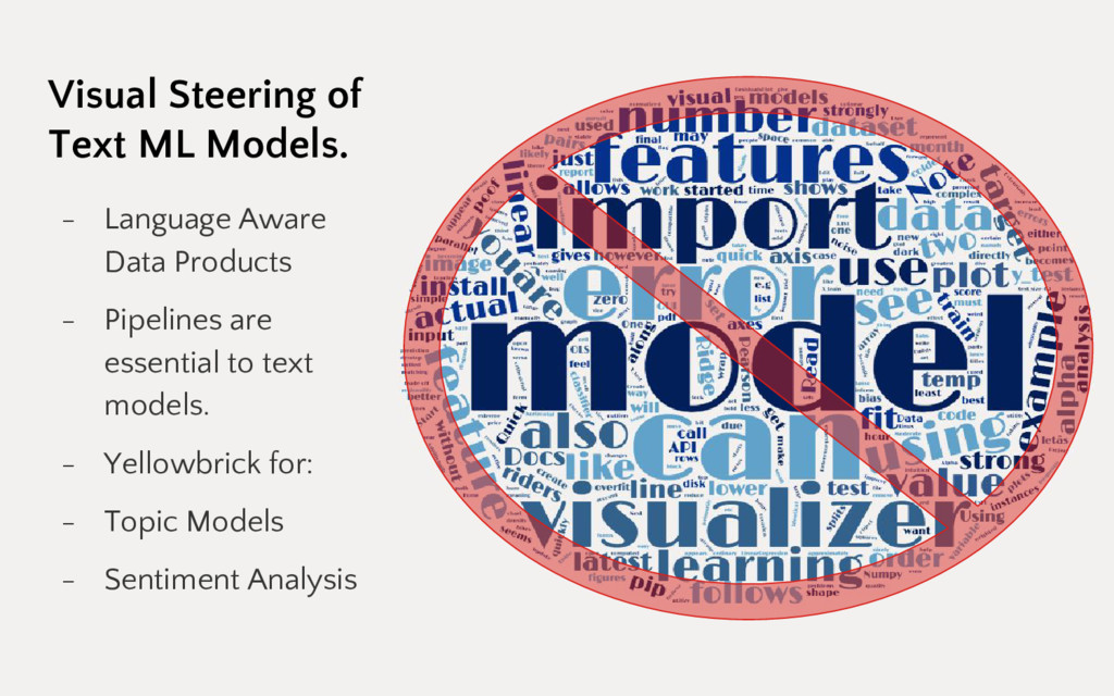
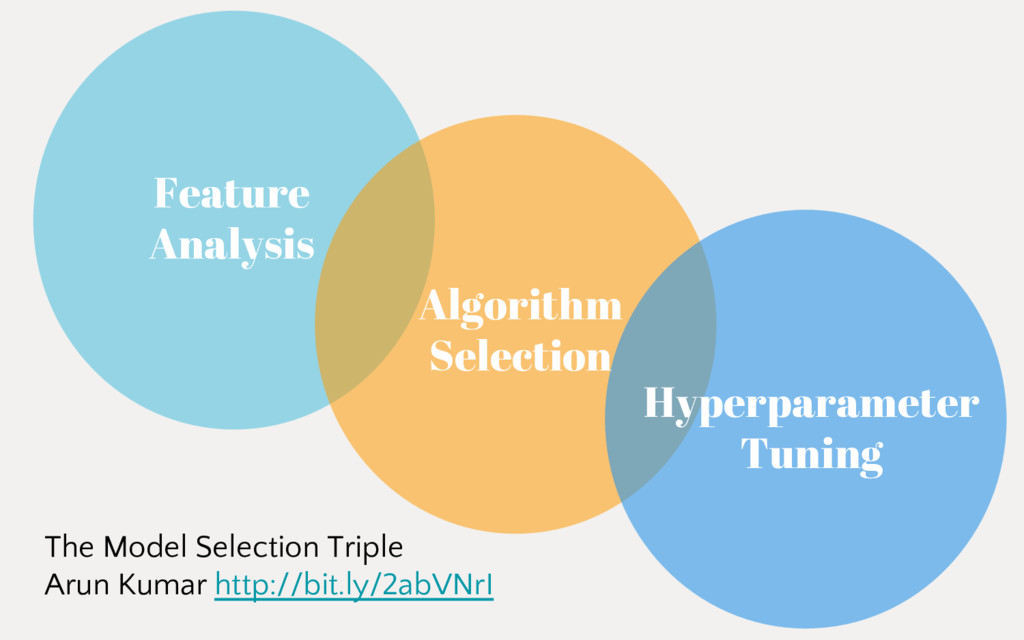
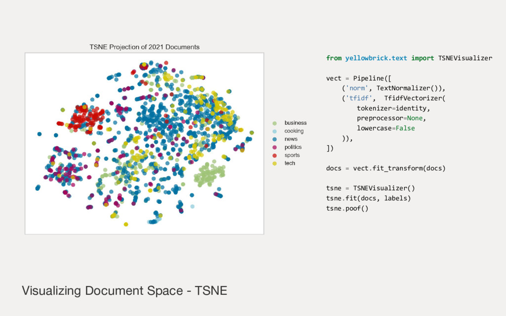
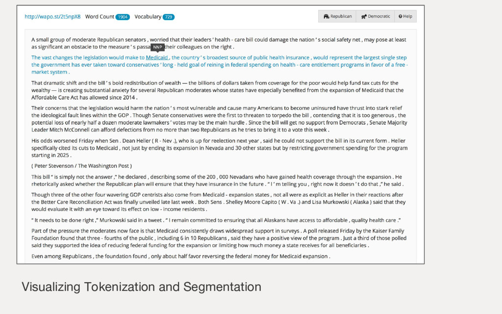
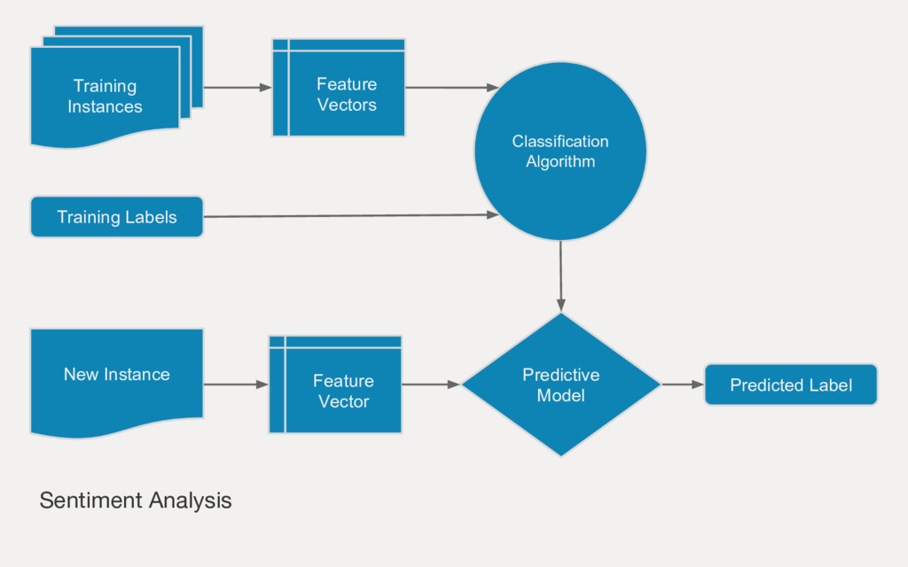
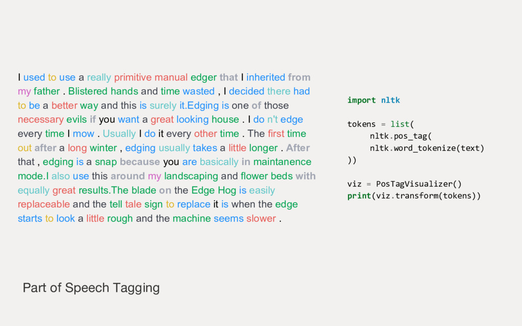
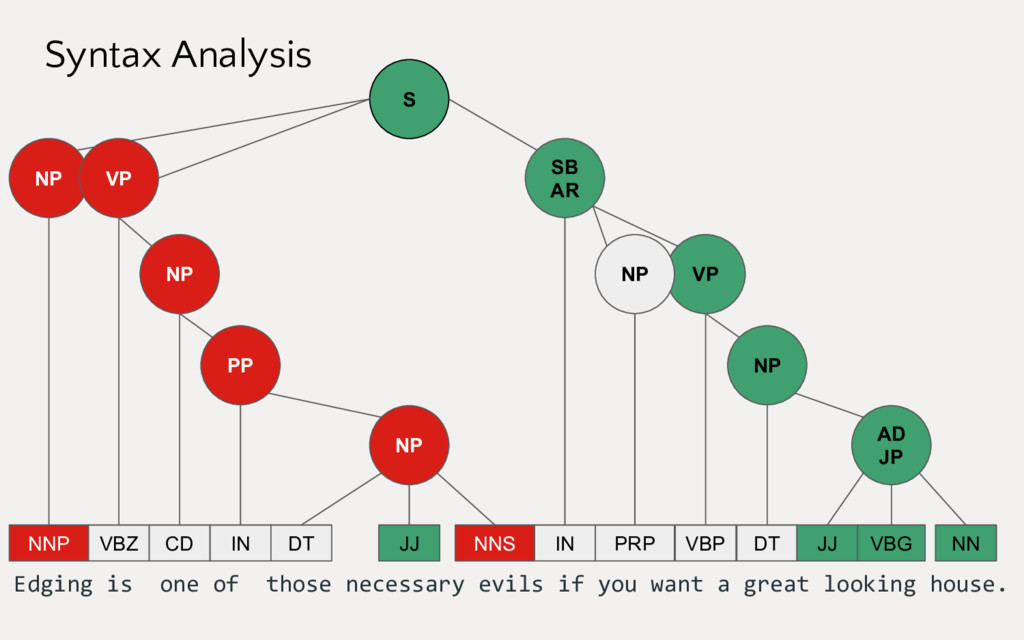
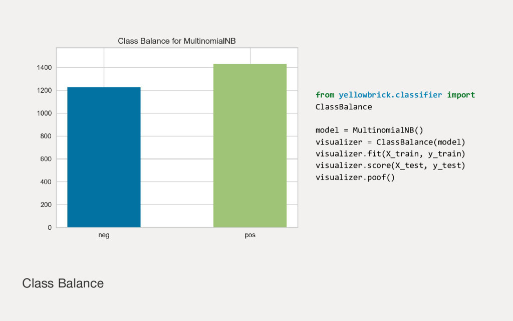
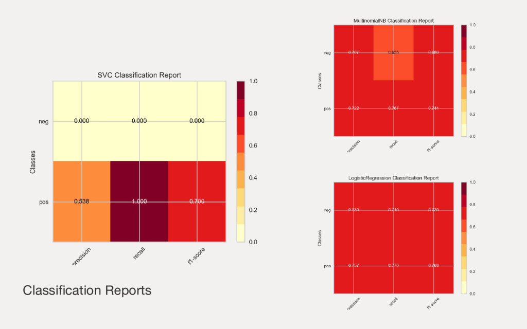
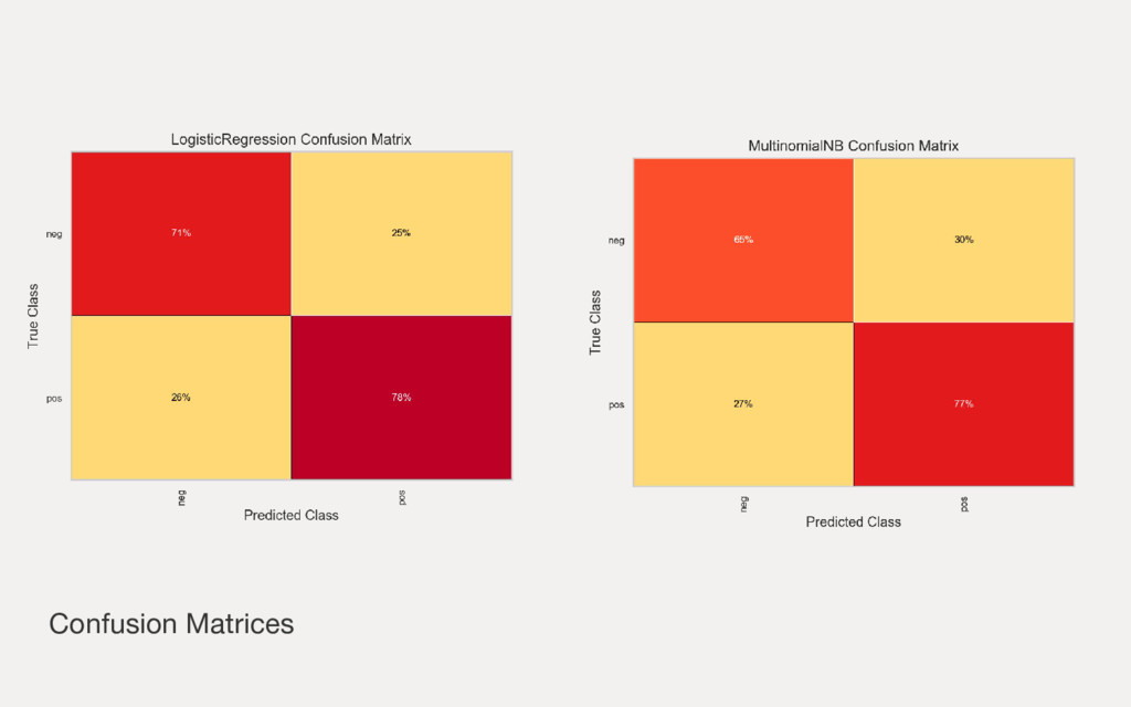
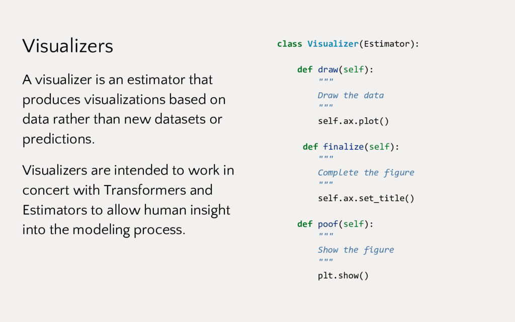
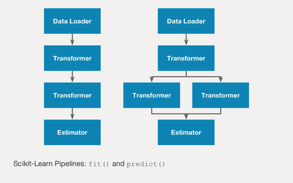
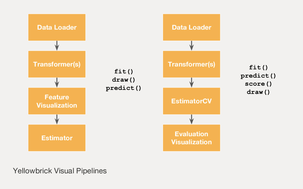
Employing machine learning in practice is half search, half expertise, and half blind luck. In this talk we will explore how to make the luck half less blind by using visual pipelines to steer model selection from raw input to operational prediction. We will look specifically at extending transformer pipelines with visualizers for sentiment analysis and topic modeling text corpora.

Transcript

1. Visual Pipelines for Text Analysis Benjamin Bengfort District Data Labs
2. Visual Steering of Text ML Models. - Language Aware Data Products - Pipelines are essential to text models. - Yellowbrick for: - Topic Models - Sentiment Analysis
3. Natural Language Understanding (AI) Models for semantic understanding, reasoning, and generation of natural languages for human-computer interaction. Computational Linguistics (NLP) Approaches to demonstrate how humans interpret and understand language and show how languages evolve. Language Aware Data Products are Not Necessarily
4. Sidebar: An Academic Context input projection hidden layer output layer Language Models and Perplexity Information Extraction/Retrieval
5. Text Models
6. Instances = Documents or Utterances (no matter their size)
7. Text as Features in Machine Learning Is “Bag of Words” a bad thing? - Discourse Features - Syntactic Features - Morphological Features - N-Grams - Grammar Extracted Phrases - Named Entities - Chunks
8. Vectorization 0 at 2 bat 1 can 0 door 1 echolocation 0 elephant 0 of 0 open 0 potato 2 see 0 she 1 sight 1 sneeze 0 studio 1 the 0 to 1 via 0 w onder The elephant sneezed at the sight of potatoes. Bats can see via echolocation. See the bat sight sneeze! Wondering, she opened the door to the studio.
9. High Dimensional Space! Baleen sample contains 2,021 files in 6 categories. Structured as: 36,816 paragraphs (18.217 mean paragraphs per file) 61,597 sentences (1.673 mean sentences per paragraph). Word count of 1,365,829 with a vocabulary of 51,227 (26.662 lexical diversity). Corpus scan took 2.7726128101348877 seconds. Reductions: - Lemmatization, Stemming - Truncation - Dimensionality Reduction - Embeddings
10. We’re doing feature engineering! pipeline = Pipeline([ ('vect', CountVectorizer()), ('tfidf', TfidfTransformer()), ('svd', TruncatedSVD()), ('model', SGDClassifier()), ]) parameters = { 'vect__max_df': (0.5, 0.75, 1.0), 'vect__max_features': (None, 5000, 10000), 'tfidf__use_idf': (True, False), 'tfidf__norm': ('l1', 'l2'), 'svd__n_components': (500, 1000, 2000, 5000), 'model__alpha': (0.00001, 0.000001), 'model__penalty': ('l2', 'elasticnet'), } search = GridSearchCV(pipeline, parameters) search.fit(X, y)
11. Data Loader Text Normalization Text Vectorization Feature Decomposition Estimator Data Loader Feature Union Pipeline Estimator Text Normalization Document Features Text Extraction Summary Vectorization Article Vectorization Concept Features Metadata Features Dict Vectorizer Text Pipelines
12. - Naive Bayes (FAST) - Maximum Entropy (Logistic Regression) - SVMs (usually linear) or SGD - RBMs - Perceptrons Commonly Used Models - Hidden Markov Models - LDA/LSA - DBSCAN/Birch - KMeans
13. The Model Selection Triple Arun Kumar http://bit.ly/2abVNrI Feature Analysis Algorithm Selection Hyperparameter Tuning
14. Visual Steering
15. The basic text visualization is … from yellowbrick.text import FrequencyVisualizer from sklearn.feature_extraction.text import CountVectorizer vect = CountVectorizer() docs = vect.fit_transform(docs) viz = FrequencyVisualizer( features=vect.get_feature_names() ) viz.fit(docs) viz.poof()
16. J. Heer and B. Shneiderman, “Interactive dynamics for visual analysis,” Queue, vol. 10, no. 2, p. 30, 2012. The Visual Analytics Mantra Overview First Zoom and Filter Details on Demand
17. Conditional Frequency by Label from yellowbrick.text import FrequencyVisualizer from sklearn.feature_extraction.text import CountVectorizer vect = CountVectorizer() docs = vect.fit_transform(docs) viz = FrequencyVisualizer( features=vect.get_feature_names() ) viz.fit(docs, labels) viz.poof()
18. “TED Word Flows” Santiago Ortiz
19. Topic Modeling
20. Topic Modeling Training Text, Documents Feature Vectors Clustering Algorithm New Document Feature Vector Topic A Topic B Topic C Similarity
21. Topic #0 â jim abenomics japan japanese rickards institution reckoning q please Topic #1 favoriting weidenhammer udacity daydream allo marks thrun raby seo aquafaba Topic #2 kearny secaucus crowhurst 2015â stringer loopholes skylineâ billowing newark hoboken Topic #3 megayachts mischa lovekin superyacht cw_anderson enchanted flickrallen sevigny zeppelin chloe Topic #4 yotel hubspot unplugged disrupted benioff maranhã lenã maranhenses vitormarigoduring quora ... Topic #10 github zube dewalt combinator jira scrum 42floors zendesk logins zenhub The Basic Topic Model - LDA from sklearn.feature_extraction.text import TfidfVectorizer from sklearn.decomposition import LatentDirichletAllocation as LDA model = Pipeline([ ('norm', TextNormalizer()), ('tfidf', TfidfVectorizer( tokenizer=identity, preprocessor=None, lowercase=False )), ('lda', LDA(n_topics=50)), ])
22. Topic feature importance distributions!
23. Visualizing Topic Space - Projections TF-IDF Vectors Frequency Vectors
24. Comparing Topics: PyLDAViz for Interactive Exploration
25. Visualizing Document Space - TSNE from yellowbrick.text import TSNEVisualizer vect = Pipeline([ ('norm', TextNormalizer()), ('tfidf', TfidfVectorizer( tokenizer=identity, preprocessor=None, lowercase=False )), ]) docs = vect.fit_transform(docs) tsne = TSNEVisualizer() tsne.fit(docs, labels) tsne.poof()
26. Spherical Topics with K-Means Text is typically very sparse. However, with a different distance metric that’s spherical, we can regain density: - Cosine - Jaccard - Soundex Opening up the possibility to using other clustering algorithms effectively.
27. Selecting K: Elbow Curves from sklearn.cluster import MiniBatchKMeans from yellowbrick.cluster import KElbowVisualizer viz = KElbowVisualizer( MiniBatchKMeans(), k=20 ) viz.fit(Xt.toarray()) viz.poof()
28. Selecting K - Silhouette Scores from yellowbrick.cluster import SilhouetteVisualizer viz = SilhouetteVisualizer(KMeans(12)) viz.fit(Xt.toarray()) viz.poof()
29. Sentiment Analysis
30. Visualizing Tokenization and Segmentation
31. Sentiment Analysis Training Instances Training Labels Feature Vectors Classification Algorithm New Instance Feature Vector Predictive Model Predicted Label
32. “Edging is one of those necessary evils if you want a great looking house. Blistered hands and time wasted, I decided there had to be a better way and this is surely it.”
33. Part of Speech Tagging I used to use a really primitive manual edger that I inherited from my father . Blistered hands and time wasted , I decided there had to be a better way and this is surely it.Edging is one of those necessary evils if you want a great looking house . I do n't edge every time I mow . Usually I do it every other time . The first time out after a long winter , edging usually takes a little longer . After that , edging is a snap because you are basically in maintanence mode.I also use this around my landscaping and flower beds with equally great results.The blade on the Edge Hog is easily replaceable and the tell tale sign to replace it is when the edge starts to look a little rough and the machine seems slower . import nltk tokens = list( nltk.pos_tag( nltk.word_tokenize(text) )) viz = PosTagVisualizer() print(viz.transform(tokens))
34. Syntax Analysis Edging is one of those necessary evils if you want a great looking house. NNP VBZ CD IN DT JJ NNS IN PRP VBP DT NN JJ VBG NP AD JP NP PP NP NP VP VP NP SB AR S
35. Class Balance from yellowbrick.classifier import ClassBalance model = MultinomialNB() visualizer = ClassBalance(model) visualizer.fit(X_train, y_train) visualizer.score(X_test, y_test) visualizer.poof()
36. Classification Reports
37. Confusion Matrices
38. ROC/AUC Curves
39. Yellowbrick
40. Yellowbrick at a Glance • Extend the Scikit-Learn API. • Enhance the model selection process. • Tools for feature visualization, visual diagnostics, and visual steering. • Visualize the model space
41. The Scikit-Learn API Buitinck, Lars, et al. "API design for machine learning software: experiences from the scikit-learn project." arXiv preprint arXiv:1309.0238 (2013). class Estimator(object): def fit(self, X, y=None): """ Fits estimator to data. """ # set state of self return self def predict(self, X): """ Predict response of X """ # compute predictions pred return pred class Transformer(Estimator): def transform(self, X): """ Transforms the input data. """ # transform X to X_prime return X_prime class Pipeline(Transfomer): @property def named_steps(self): """ Returns a sequence of estimators """ return self.steps @property def _final_estimator(self): """ Terminating estimator """ return self.steps[-1]
42. The Matplotlib API The matplotlib API combines two primary components: - pyplot: procedural descriptions of visualization. - artists: object oriented construction of visual elements. Drawing occurs globally and renders on demand.
43. The trick: combine functional/procedural matplotlib + object-oriented Scikit-Learn. Yellowbrick
44. Visualizers A visualizer is an estimator that produces visualizations based on data rather than new datasets or predictions. Visualizers are intended to work in concert with Transformers and Estimators to allow human insight into the modeling process. class Visualizer(Estimator): def draw(self): """ Draw the data """ self.ax.plot() def finalize(self): """ Complete the figure """ self.ax.set_title() def poof(self): """ Show the figure """ plt.show()
45. Scikit-Learn Pipelines: fit() and predict() Data Loader Transformer Transformer Estimator Data Loader Transformer Transformer Estimator Transformer
46. Yellowbrick Visual Pipelines Data Loader Transformer(s) Feature Visualization Estimator fit() draw() predict() Data Loader Transformer(s) EstimatorCV Evaluation Visualization fit() predict() score() draw()
47. Model Selection Pipelines Multi-Estimator Visualization Data Loader Transformer(s) Estimator Estimator Estimator Estimator Cross Validation Cross Validation Cross Validation Cross Validation
48. Contributions Welcome!