Upgrade to Pro — share decks privately, control downloads, hide ads and more …

Master_ATSI_Univ_Paris_Sacly 3

Djafari
January 11, 2018
20

Master_ATSI_Univ_Paris_Sacly 3

Teaching Master courses at Univ. Paris Saclay
"Multi-componets Data, Signal and Image Processing for Biological and Medical Applications". Part 3

Djafari

January 11, 2018
Tweet

Transcript

  1. . Multi-componets Data, Signal and Image Processing for Biological and

    Medical Applications Ali Mohammad-Djafari Laboratoire des Signaux et Syst` emes UMR 8506 CNRS - CS - Univ Paris Sud CentraleSup´ elec, Gif-sur-Yvette. [email protected] http://djafari.free.fr January 6, 2017 A. Mohammad-Djafari, Data, signals, images in Biological and medicalapplication. Master ATSI, UPSa, 2015-2016, Gif, France, 1/40
  2. Summary 3: Two inverse problems ◮ Deconvolution ◮ Computed Tomography

    A. Mohammad-Djafari, Data, signals, images in Biological and medicalapplication. Master ATSI, UPSa, 2015-2016, Gif, France, 2/40
  3. Case study: Signal deconvolution ◮ Convolution, Identification and Deconvolution ◮

    Forward and Inverse problems: Well-posedness and Ill-posedness ◮ Naˆ ıve methods of Deconvolution ◮ Classical methods: Wiener filtering ◮ Bayesian approach to deconvolution ◮ Simple and Blind Deconvolution ◮ Deterministic and probabilistic methods ◮ Joint source and canal estimation A. Mohammad-Djafari, Data, signals, images in Biological and medicalapplication. Master ATSI, UPSa, 2015-2016, Gif, France, 3/40
  4. Convolution, Identification and deconvolution f(t) ✲ h(t) ✲ ♠ +

    ❄ ǫ(t) ✲g(t) g(t) = f(t′) h(t − t′) dt′ + ǫ(t) = h(t′) f(t − t′) dt′ + ǫ(t) ◮ Convolution: Given f and h compute g ◮ Identification: Given f and g estimate h ◮ Deconvolution: Given g and h estimate f ◮ Blind deconvolution: Given g estimate both h and f A. Mohammad-Djafari, Data, signals, images in Biological and medicalapplication. Master ATSI, UPSa, 2015-2016, Gif, France, 4/40
  5. Convolution: Given f and h compute g ◮ Direct computation:

    g=conv(h,f) ◮ Fourier domain: g(t) = h(t) ∗ f(t) −→ G(ω) = H(ω)F(ω) ◮ Compute H(ω), F(ω) and G(ω) = H(ω)F(ω) ◮ Compute g(t) by inverse FT of G(ω) ◮ Take care of dimensions and boarder effects. A. Mohammad-Djafari, Data, signals, images in Biological and medicalapplication. Master ATSI, UPSa, 2015-2016, Gif, France, 5/40
  6. Convolution: Discretization f(t) ✲ h(t) ✲ ♠ + ❄ ǫ(t)

    ✲g(t) g(t) = f(t′) h(t − t′) dt′ + ǫ(t) = h(t′) f(t − t′) dt′ + ǫ(t) ◮ The signals f(t), g(t), h(t) are discretized with the same sampling period ∆T = 1, ◮ The impulse response is finite (FIR) : h(t) = 0, for t such that t < −q∆T or ∀t > p∆T. g(m) = p k=−q h(k) f(m − k) + ǫ(m), m = 0, · · · , M A. Mohammad-Djafari, Data, signals, images in Biological and medicalapplication. Master ATSI, UPSa, 2015-2016, Gif, France, 6/40
  7. Convolution: Discretized matrix vector forms     

                            g(0) g(1) . . . . . . . . . . . . . . . . . . g(M)                              =                            h(p) · · · h(0) · · · h(−q) 0 · · · · · · · · · 0 0 . . . . . . . . . . . . . . . . . . . . . h(p) · · · h(0) · · · h(−q) . . . . . . . . . . . . . . . . . . . . . . . . . . . 0 0 · · · · · · 0 h(p) · · · h(0) · · · h(−q)                                                               f(−p) . . . f(0) f(1) . . . . . . . . . . . . f(M) f(M + 1) . . . f(M + q)                                    g = Hf + ǫ ◮ g is a (M + 1)-dimensional vector, ◮ f has dimension M + p + q + 1, ◮ h = [h(p), · · · , h(0), · · · , h(−q)] has dimension (p + q + 1) ◮ H has dimensions (M + 1) × (M + p + q + 1). A. Mohammad-Djafari, Data, signals, images in Biological and medicalapplication. Master ATSI, UPSa, 2015-2016, Gif, France, 7/40
  8. Convolution: Discretized matrix vector form ◮ If system is causal

    (q = 0) we obtain               g(0) g(1) . . . . . . . . . . . . g(M)               =                h(p) · · · h(0) 0 · · · · · · 0 0 . . . . . . . . . . . . h(p) · · · h(0) . . . . . . . . . . . . 0 0 · · · · · · 0 h(p) · · · h(0)                                   f(−p) . . . f(0) f(1) . . . . . . . . . . . . f(M)                    ◮ g is a (M + 1)-dimensional vector, ◮ f has dimension M + p + 1, ◮ h = [h(p), · · · , h(0)] has dimension (p + 1) ◮ H has dimensions (M + 1) × (M + p + 1). A. Mohammad-Djafari, Data, signals, images in Biological and medicalapplication. Master ATSI, UPSa, 2015-2016, Gif, France, 8/40
  9. Convolution: Causal systems and causal input    

              g(0) g(1) . . . . . . . . . . . . g(M)               =               h(0) h(1) ... . . . h(p) · · · h(0) 0 ... ... . . . 0 · · · 0 h(p) · · · h(0)                             f(0) f(1) . . . . . . . . . . . . f(M)               ◮ g is a (M + 1)-dimensional vector, ◮ f has dimension M + 1, ◮ h = [h(p), · · · , h(0)] has dimension (p + 1) ◮ H has dimensions (M + 1) × (M + 1). A. Mohammad-Djafari, Data, signals, images in Biological and medicalapplication. Master ATSI, UPSa, 2015-2016, Gif, France, 9/40
  10. Convolution, Identification, Deconvolution and Blind deconvolution problems g(t) = f(t′)

    h(t − t′) dt′ + ǫ(t) = h(t′) f(t − t′) dt′ + ǫ(t) f(t)✲ h(t) ✲ ❥ + ❄ ǫ(t) ✲g(t) f(t)✲ h(t) ✲ ❥ + ❄ ǫ(t) ✲g(t) F(ω)✲ H(ω) ✲ ❥ + ❄ E(ω) ✲ G(ω) F(ω)✲ H(ω) ✲ ❥ + ❄ E(ω) ✲ G(ω) G(ω) = H(ω) F(ω) + E(ω) G(ω) = H(ω) F(ω) + E(ω) F(ω) = G(ω) H(ω) + E(ω) H(ω) H(ω) = G(ω) F(ω) + E(ω) F(ω) ◮ Convolution: Given h and f compute g ◮ Identification: Given f and g estimate h ◮ Simple Deconvolution: Given h and g estimate f ◮ Blind Deconvolution: Given g estimate h and f A. Mohammad-Djafari, Data, signals, images in Biological and medicalapplication. Master ATSI, UPSa, 2015-2016, Gif, France, 10/40
  11. Deconvolution: Given g and h estimate f ◮ Direct computation:

    f=deconv(g,h) ◮ Fourier domain: Inverse Filtering F(ω) = G(ω) H(ω) ◮ Compute H(ω), G(ω) and F(ω) = G(ω) H(ω) ◮ Compute g(t) by inverse FT of F(ω) ◮ Main difficulties: Divide by zero and noise amplification A. Mohammad-Djafari, Data, signals, images in Biological and medicalapplication. Master ATSI, UPSa, 2015-2016, Gif, France, 11/40
  12. Identification: Given g and f estimate h ◮ Direct computation:

    ◮ f(t) = δ(t) −→ g(t) = h(t) −→ h(t) = g(t) ◮ f(t) = 0 t < 0 1 t > 0 −→ g(t) = t 0 h(t) dt −→ h(t) = ∂g(t) ∂t ◮ Fourier domain: Inverse Filtering H(ω) = G(ω) F(ω) ◮ Compute F(ω), G(ω) and H(ω) = G(ω) F(ω) ◮ Compute h(t) by inverse FT of H(ω) ◮ Main difficulties: Divide by zero and noise amplification A. Mohammad-Djafari, Data, signals, images in Biological and medicalapplication. Master ATSI, UPSa, 2015-2016, Gif, France, 12/40
  13. Convolution in 1D and 2D: Signal deconvolution and Image restoration

    f(t) −→ h(t) −→ ǫ(t) ↓ −→ g(t) g(t) = f(t′) h(t − t′) dt′ + ǫ(t) ◮ f(t), g(t) and ǫ(t) are modelled as Gaussian random signal f(x, y) −→ h(x, y) −→ ǫ(x, y) ↓ −→ g(x, y) g(x, y) = f(x′, y′) h(x − x′, y − y′) dx′ dy′ + ǫ(x, y) ◮ f(x, y), g(x, y) and ǫ(x, y) are modelled as homogeneous and Gaussian random fields A. Mohammad-Djafari, Data, signals, images in Biological and medicalapplication. Master ATSI, UPSa, 2015-2016, Gif, France, 13/40
  14. Wiener Filtering f(t) ✲ h(t) ✲ ✒✑ ✓✏ + ❄

    ǫ(t) ✲ g(t) E {g(t)} = h(t) ∗ E {f(t)} + E {ǫ(t)} Rgg(τ) = h(t) ∗ h(t) ∗ Rff (τ) + Rǫǫ (τ) Rgf (τ) = h(t) ∗ Rff (τ) Sgg(ω) = |H(ω)|2Sff (ω) + Rǫǫ (ω) Sgf (ω) = H(ω)Sff (ω) Sfg (ω) = H∗(ω)Sff (ω) g(t) ✲ W(ω) ✲ f(t) f(t) = w(t) ∗ g(t) A. Mohammad-Djafari, Data, signals, images in Biological and medicalapplication. Master ATSI, UPSa, 2015-2016, Gif, France, 14/40
  15. Wiener Filtering EQM = E [f(t) − f(t)]2 = E

    [f(t) − w(t) ∗ g(t)]2 ∂EQM ∂f = −2E {[f(t) − w(t) ∗ g(t)] ∗ g(t + τ)} = 0 E {[f(t) − w(t) ∗ g(t)] g(t + τ)} = 0 ∀t, τ −→ Rfg (τ) = w(t) ∗ Rgg(τ) W(ω) = Sfg (ω) Sgg(ω) = H∗(ω) Sff (ω) |H(ω)|2 Sff (ω) + Sǫǫ (ω) W(ω) = H∗(ω)Sff (ω) |H(ω)|2Sff (ω) + Sǫǫ (ω) = 1 H(ω) |H(ω)|2 |H(ω)|2 + S ǫǫ (ω) Sff (ω) A. Mohammad-Djafari, Data, signals, images in Biological and medicalapplication. Master ATSI, UPSa, 2015-2016, Gif, France, 15/40
  16. Wiener Filtering ◮ Linear Estimation: f(x, y) is such that:

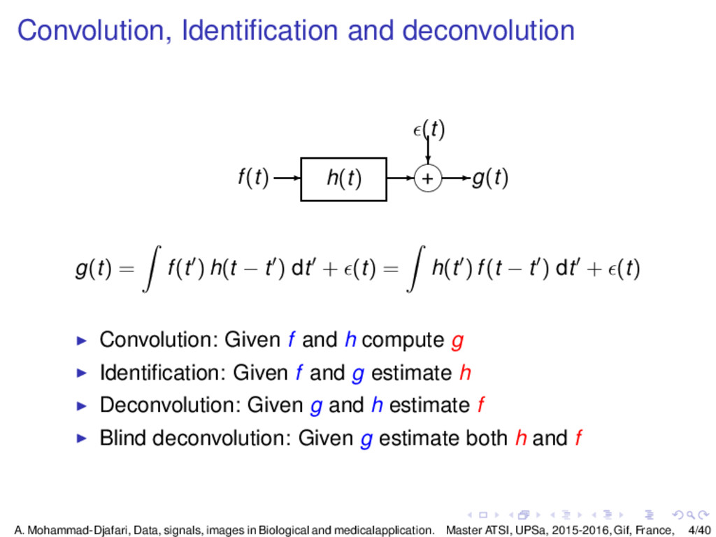
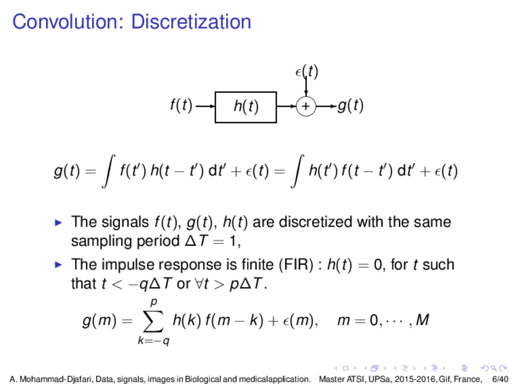
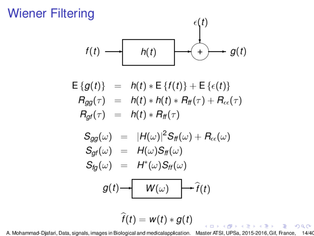
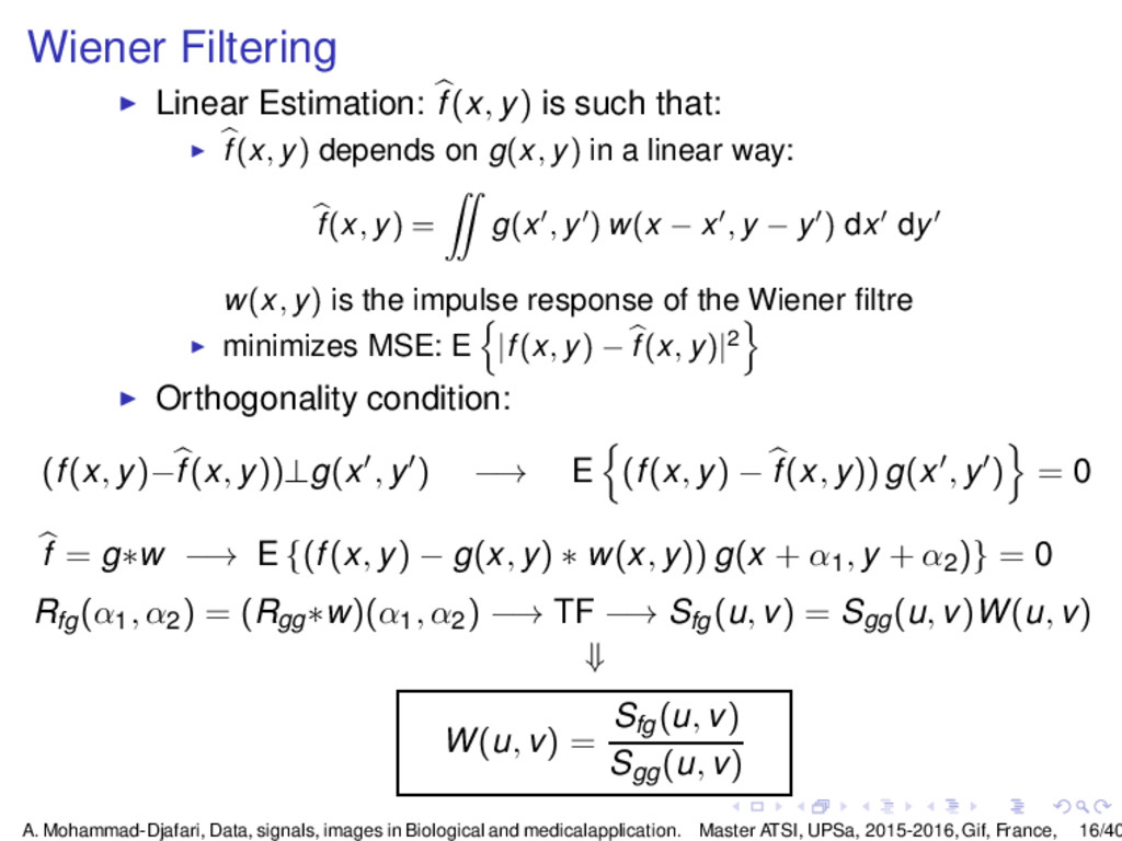
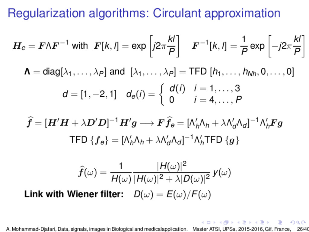
    ◮ f(x, y) depends on g(x, y) in a linear way: f(x, y) = g(x′, y′) w(x − x′, y − y′) dx′ dy′ w(x, y) is the impulse response of the Wiener filtre ◮ minimizes MSE: E |f(x, y) − f(x, y)|2 ◮ Orthogonality condition: (f(x, y)−f (x, y))⊥g(x′, y′) −→ E (f(x, y) − f(x, y)) g(x′, y′) = 0 f = g∗w −→ E {(f(x, y) − g(x, y) ∗ w(x, y)) g(x + α1 , y + α2 )} = 0 Rfg (α1 , α2 ) = (Rgg ∗w)(α1 , α2 ) −→ TF −→ Sfg (u, v) = Sgg(u, v)W(u, v) ⇓ W(u, v) = Sfg (u, v) Sgg(u, v) A. Mohammad-Djafari, Data, signals, images in Biological and medicalapplication. Master ATSI, UPSa, 2015-2016, Gif, France, 16/40
  17. Wiener filtering Signal Image W(ω) = Sfg (ω) Sgg(ω) W(u,

    v) = Sfg (u, v) Sgg(u, v) Particular Case: f(x, y) and b(x, y) are assumed to be centered and non correlated Sfg (u, v) = H′(u, v) Sff (u, v) Sgg(u, v) = |H(u, v)|2 Sff (u, v) + Sǫǫ (u, v) W(u, v) = H′(u, v)Sff (u, v) |H(u, v)|2Sff (u, v) + Sǫǫ (u, v) Signal Image W(ω) = 1 H(ω) |H(ω)|2 |H(ω)|2 + S ǫǫ (ω) Sff (ω) W(u, v) = 1 H(u, v) |H(u, v)|2 |H(u, v)|2 + S ǫǫ (u,v) Sff (u,v) A. Mohammad-Djafari, Data, signals, images in Biological and medicalapplication. Master ATSI, UPSa, 2015-2016, Gif, France, 17/40
  18. Convolution: Discretization for Identification Causal systems and causal input 

                    g(0) g(1) . . . . . . . . . . . . . . . g(M)                  =                 0 . 0 f(0) . . f(0) f(1) . f(0) f(1) . . . . . . . . . . f(0) f(1) f(M − p) f(1) . . . . . . . . . . . . f(M − p) . . . f(M)                           h(p) h(p − 1) . . . . . . h(1) h(0)           g = F h + ǫ ◮ g is a (M + 1)-dimensional vector, ◮ F has dimension (M + 1) × (p + 1), A. Mohammad-Djafari, Data, signals, images in Biological and medicalapplication. Master ATSI, UPSa, 2015-2016, Gif, France, 18/40
  19. Algebraic Approches Signal Image f(t) −→ h(t) −→ g(t) f(x,

    y) −→ h(x, y) −→ g(x, y) Discretization ⇓ g = Hf ◮ Ideal case: H invertible −→ f = H−1g ◮ M > N Least Squares: g = Hf + ǫ e = g − Hf 2 = [g − Hf]′[g − Hf] f = arg min f {e} ∇e = −2H′[g − Hf] = 0 −→ H′Hf = H′g ◮ If H′H is invertible f = (H′H)−1H′g A. Mohammad-Djafari, Data, signals, images in Biological and medicalapplication. Master ATSI, UPSa, 2015-2016, Gif, France, 19/40
  20. Algebraic Approches: Generalized Inversion General case of [M, N] matrix

    H: ◮ if M = N and rang {H} = N then H+ = H−1 ◮ if M > N and rang {H} = N then H+ = (H′H)−1H′ ◮ if M < N and rang {H} = M then H+ = H′(HH′)−1 ◮ if rang {H} = K < inf M, N then ◮ Singular Value Decomposition (SVD) ◮ Iterative methods ◮ Recursive methods A. Mohammad-Djafari, Data, signals, images in Biological and medicalapplication. Master ATSI, UPSa, 2015-2016, Gif, France, 20/40
  21. Regularization Jλ (f) = [Hf−g]′[Hf−g]+λ[Df]′[Df] = Hf−g 2+λ Df 2

    D =            1 0 · · · · · · 0 −1 1 ... . . . 0 −1 1 ... . . . 0 −1 1 ... 0 0 −1 1            or D =            1 0 · · · · · · 0 −2 1 ... . . . 1 −2 1 ... . . . 1 −2 1 ... 0 1 −2 1 ∇Jλ = 2H′[Hf − g]′ + 2λD′Df = 0 [H′H + λD′D]f = H′g −→ f = [H′H + λD′D]−1H′g A. Mohammad-Djafari, Data, signals, images in Biological and medicalapplication. Master ATSI, UPSa, 2015-2016, Gif, France, 21/40
  22. Regularization Algorithmes minimize J(f) = Q(f) + λΩ(f) with Q(f)

    = g − Hf 2 = [g − Hf]′[g − Hf] = minimize Ω(f) subj. to the constraint e = g − Hf 2 = [g − Hf]′[g − Hf] < ǫ A priori Information: ◮ Smoothnesse Ω(f) = [Df]′[Df] = Df 2 f = [H′H + λD′D]−1H′g ◮ Positivity: Ω(f) = a nonquadratique function of f No explicite solution A. Mohammad-Djafari, Data, signals, images in Biological and medicalapplication. Master ATSI, UPSa, 2015-2016, Gif, France, 22/40
  23. Regularization Algorithmes: 3 main approaches f = [H′H + λD′D]−1H′g

    Computation of f = [H′H + λD′D]−1H′g ◮ Circulante matrix approximation: when H and D are Toeplitz, they can be approximated by the circulant matrices ◮ Iterative methods: f = arg min f J(f) = g − Hf 2 + λDf 2 ◮ Recursive methods: f at iteration k is computed as a function of f at previous iteration with one less data. A. Mohammad-Djafari, Data, signals, images in Biological and medicalapplication. Master ATSI, UPSa, 2015-2016, Gif, France, 23/40
  24. Regularization algorithms: Circulant approximation 1D Deconvolution: g = H f

    + ǫ H Toeplitz matrix f = arg min f {f} J(f) = Q(f) + λΩ(f) Q(f) = g−Hf 2 = [g−Hf]′[g−Hf] and Ω(f) = Df 2 = [Df]′[D C a convolution matrix with the following impulse response h1 = [1, −2, 1] −→ x(i) = x(i + 1) − 2x(i) + x(i − 1) Ω(f) = N j=1 (x(i + 1) − 2x(i) + x(i − 1))2 = Df 2 = f′D′Df Solution : f = [H′H + λC′C]−1H′g A. Mohammad-Djafari, Data, signals, images in Biological and medicalapplication. Master ATSI, UPSa, 2015-2016, Gif, France, 24/40
  25. Regularization algorithms: Circulant approximation Main Idea : expand the vectors

    f, h and g by the zeros to obtain ge = Hefe with He a circulante matrix fe(i) = f(i) i = 1, . . . , N 0 i = N + 1, . . . , P ≥ N + Nh − 1 ge(i) = g(i) i = 1, . . . , M 0 i = M + 1, . . . , P he(i) = h(i) i = 1, . . . , Nh 0 i = Nh + 1, . . . , P ge(k) = Nh−1 i=0 fe(k − i)he(i) −→ ge = Hefe with He a circulante matrix whcich can diagonalized by FFT A. Mohammad-Djafari, Data, signals, images in Biological and medicalapplication. Master ATSI, UPSa, 2015-2016, Gif, France, 25/40
  26. Regularization algorithms: Circulant approximation He = F ΛF −1 with

    F [k, l] = exp j2π kl P F −1[k, l] = 1 P exp −j2π kl P Λ = diag[λ1 , . . . , λP ] and [λ1 , . . . , λP ] = TFD [h1 , . . . , hNh , 0, . . . , 0] d = [1, −2, 1] de(i) = d(i) i = 1, . . . , 3 0 i = 4, . . . , P f = [H′H + λD′D]−1H′g −→ F fe = [Λ′ h Λh + λΛ′ d Λd ]−1Λ′ h F g TFD {fe } = [Λ′ h Λh + λΛ′ d Λd ]−1Λ′ h TFD {g} f(ω) = 1 H(ω) |H(ω)|2 |H(ω)|2 + λ|D(ω)|2 y(ω) Link with Wiener filter: D(ω) = E(ω)/F(ω) A. Mohammad-Djafari, Data, signals, images in Biological and medicalapplication. Master ATSI, UPSa, 2015-2016, Gif, France, 26/40
  27. Image Restoration C Convolution matrix with the following impulse response:

    H1 =   0 1 0 1 −4 1 0 1 0   Ω(f) = (f(i + 1, j) + f(i − 1, j) +f(i + 1, j + 1) + f(i − 1, j + 1) − 4f(i, j))2 fe(k, l) = f(k, l) k = 1, . . . , K l = 1, . . . , L 0 k = K + 1, . . . , P l = L + 1, . . . , P A. Mohammad-Djafari, Data, signals, images in Biological and medicalapplication. Master ATSI, UPSa, 2015-2016, Gif, France, 27/40
  28. Regularization: Iterative methods: Gradient based f = arg min f

    {J(f) = Q(f) + λΩ(f)} Let note : gk = ∇J fk gradient, Hk = ∇2J fk Hessien. First order gradient methods ◮ fixed step: f(k+1) = f(k) + αg(k) α fixe ◮ Optimal or steepest descente step: f(k+1) = f(k) + α(k)g(k) α(k) = − g(k)t g(k) g(k)t Hk g(k) = ||gk 2 gk 2 H A. Mohammad-Djafari, Data, signals, images in Biological and medicalapplication. Master ATSI, UPSa, 2015-2016, Gif, France, 28/40
  29. Regularization: Iterative methods: Conjugate Gradient ◮ Conjugate Gradient (CG) f(k+1)

    = f(k) + α(k)d(k) α(k) = − d(k)t g(k) d(k)t Hk d(k) d(k+1) = d(k) + β(k)g(k) β(k) = − g(k)t g(k) g(k−1)t g(k−1) ◮ Newton method f(k+1) = f(k) + (H(k))−1g(k) ◮ Advantages : Ω(f) can be any convexe function ◮ Limitations : Computational cost A. Mohammad-Djafari, Data, signals, images in Biological and medicalapplication. Master ATSI, UPSa, 2015-2016, Gif, France, 29/40
  30. Regularization: Recursive algorithms f = [H′H + λD]−1H′g Main idea:

    Express fi+1 as a function of fi fi+1 = (H′ i+1 Hi+1 + αD)−1H′ i+1 gi+1 fi = (Ht i Hi + αD)−1Ht i gi ⇓ fi+1 = (Ht i Hi + hi+1h′ i+1 + αD)−1(Ht i gi − hi+1gi + 1) Noting: Pi = (Ht i Hi + αD)−1 and P t i+1 = P t i + hi+1h′ i+1 ⇓ fi+1 = fi + Pi+1hi+1 (gi+1 − h′ i+1 fi ) Pi+1 = Pi − Pihi+1 (h′ i+1 PiHi+1 + α)−1h′ i+1 Pi A. Mohammad-Djafari, Data, signals, images in Biological and medicalapplication. Master ATSI, UPSa, 2015-2016, Gif, France, 30/40
  31. Identification and Deconvolution Deconvolution Identification g = H f +

    ǫ g = F h + ǫ J(f) = g − Hf 2 + λf Df f 2 J(h) = g − F h 2 + λh Dhh ∇J(f) = −2H′(g − Hf) + 2λf D′ f Df f ∇J(h) = −2F ′(g − F h) + 2λhD′ h f = [H′H + λf D′ f Df ]−1H′g h = [F ′F + λhD′ h Dh ]−1F ′g f(ω) = H∗(ω) |H(ω)|2+λf |Df (ω)|2 g(ω) h(ω) = |F∗(ω) |F(ω)|2+λh |Dh (ω)|2 g(ω) f(ω) = H∗(ω) |H(ω)|2+ Sǫǫ(ω) Sff (ω) g(ω) h(ω) = F∗(ω) |F(ω)|2+ Sǫǫ(ω) Shh(ω) g(ω) p(g|f) = N(Hf, Σǫ ) p(g|h) = N(F h, Σǫ ) p(f) = N(0, Σf ) p(h) = N(0, Σh ) p(f|g) = N(f, Σf ) p(h|g) = N(h, Σh ) Σf = [H′H + λf D′ f Df ]−1 Σh = [F ′F + λhD′ h Dh ]−1 f = [H′H + λf D′ f Df ]−1H′g h = [F ′F + λhD′ h Dh ]−1F ′g A. Mohammad-Djafari, Data, signals, images in Biological and medicalapplication. Master ATSI, UPSa, 2015-2016, Gif, France, 31/40
  32. Blind Deconvolution: Regularization Deconvolution Identification g = H f +

    ǫ g = F h + ǫ J(f) = g − Hf 2 + λf Df f 2 J(h) = g − F h 2 + λh Dhh 2 ◮ Joint Criterion J(f, h) = g − Hf 2 + λf Df f 2 + λh Dhh 2 ◮ iterative algorithm Deconvolution Identification ∇f J(f, h) = −2H′(g − Hf) + 2λf D′ f Df f ∇h J(f, h) = −2F ′(g − F h) + f = [H′H + λf D′ f Df ]−1H′g h = [F ′F + λhD′ h Dh ]− f(ω) = 1 H(ω) |H(ω)|2 |H(ω)|2+λf |Df (ω)|2 g(ω) f(ω) = 1 F(ω) |F(ω)|2 |F(ω)|2+λh |Dh (ω) A. Mohammad-Djafari, Data, signals, images in Biological and medicalapplication. Master ATSI, UPSa, 2015-2016, Gif, France, 32/40
  33. Blind Deconvolution: Bayesian approach Deconvolution Identification g = H f

    + ǫ g = F h + ǫ p(g|f) = N(Hf, Σǫ ) p(g|h) = N(F h, Σǫ ) p(f) = N(0, Σf ) p(h) = N(0, Σh ) p(f|g) = N(f, Σf ) p(h|g) = N(h, Σh ) Σf = [H′H + λf D′ f Df ]−1 Σh = [F ′F + λhD′ h Dh ]−1 f = [H′H + λf D′ f Df ]−1H′g h = [F ′F + λhD′ h Dh ]−1F ′g ◮ Joint posterior law: p(f, h|g) ∝ p(g|f, h) p(f) p(hh) p(f, h|g) ∝ exp [−J(f, h)] with J(f, h) = g − Hf 2 + λf Df f 2 + λh Dhh 2 ◮ iterative algorithm A. Mohammad-Djafari, Data, signals, images in Biological and medicalapplication. Master ATSI, UPSa, 2015-2016, Gif, France, 33/40
  34. Blind Deconvolution: Bayesian Joint MAP criterion ◮ Joint posterior law:

    p(f, h|g) ∝ p(g|f, h) p(f) p(hh) p(f, h|g) ∝ exp [−J(f, h)] with J(f, h) = g − Hf 2 + λf Df f 2 + λh Dhh 2 ◮ iterative algorithm Deconvolution Identification p(g|f, H) = N(Hf, Σǫ ) p(g|h, F ) = N(F h, Σǫ ) p(f) = N(0, Σf ) p(h) = N(0, Σh ) p(f|g, H) = N(f, Σf ) p(h|g, F ) = N(h, Σh ) Σf = [H′H + λf D′ f Df ]−1 Σh = [F ′F + λhD′ h Dh ]−1 f = [H′H + λf D′ f Df ]−1H′g h = [F ′F + λhD′ h Dh ]−1F ′g A. Mohammad-Djafari, Data, signals, images in Biological and medicalapplication. Master ATSI, UPSa, 2015-2016, Gif, France, 34/40
  35. Blind Deconvolution: Marginalization and EM algorithm ◮ Joint posterior law:

    p(f, h|g) ∝ p(g|f, h) p(f) p(hh) ◮ Marginalization p(h|g) = p(f, h|g) df h = arg max h {p(h|g)} −→ f = arg max f p(f|g, h) ◮ Expression of p(h|g) and its maximization are complexes ◮ Expectation-Maximization Algorithm ln p(f, h|g) ∝ J(f, h) = g−Hf 2+λf Df f 2+λh Dhh 2 ◮ Iterative algorithm ◮ Expectation: Compute Q(h, hk−1) = Ep(f,hk−1|g) {J(f, h)} = ln p(f, h|g) p(f,hk−1|g) ◮ Maximization: hk = arg max h Q(h, hk−1) A. Mohammad-Djafari, Data, signals, images in Biological and medicalapplication. Master ATSI, UPSa, 2015-2016, Gif, France, 35/40
  36. Blind Deconvolution: Variational Bayesian Approximation algorithm ◮ Joint posterior law:

    p(f, h|g) ∝ p(g|f, h) p(f) p(hh) ◮ Approximation: p(f, h|g) by q(f, h|g) = q1 (f) q2 (h) ◮ Criterion of approximation: Kullback-Leiler KL(q|p) = q ln q p = q1 q2 ln q1 q2 p KL(q1 q2 |p) = q1 ln q1 + q2 ln q2 − q ln p = −H(q1 ) − H(q2 ) + − ln p((f, h|g) q ◮ When the expression of q1 and q2 are obtained, use them. A. Mohammad-Djafari, Data, signals, images in Biological and medicalapplication. Master ATSI, UPSa, 2015-2016, Gif, France, 36/40
  37. Variational Bayesian Approximation algorithm ◮ Kullback-Leibler criterion KL(q1 q2 |p)

    = q1 ln q1 + q2 ln q2 + q ln p = −H(q1 ) − H(q2 ) + − ln p((f, h|g) q ◮ Free energy F(q1 q2 ) = − ln p((f, h|g) q1q2 ◮ Equivalence between optimization of KL(q1 q2 |p) and F(q1 q2 ) ◮ Alternate optimization: q1 = arg min q1 {KL(q1 q2 |p)} = arg min q1 {F(q1 q2 )} q2 = arg min q2 {KL(q1 q2 |p)} = arg min q2 {F(q1 q2 )} A. Mohammad-Djafari, Data, signals, images in Biological and medicalapplication. Master ATSI, UPSa, 2015-2016, Gif, France, 37/40
  38. Summary of Bayesian estimation for Deconvolution ◮ Simple Bayesian Model

    and Estimation for Deconvolution θ2 ❄ p(f|θ2 ) Prior ⋄ θ1 ❄ p(g|f, θ1 ) Likelihood −→ p(f|g, θ) Posterior −→ f ◮ Full Bayesian Model and Hyperparameter Estimation for Deconvolution ↓ α, β Hyper prior model p(θ|α, β) θ2 ❄ p(f|θ2 ) Prior ⋄ θ1 ❄ p(g|f, θ1 ) Likelihood −→p(f, θ|g, α, β) Joint Posterior −→ f −→ θ A. Mohammad-Djafari, Data, signals, images in Biological and medicalapplication. Master ATSI, UPSa, 2015-2016, Gif, France, 38/40
  39. Summary of Bayesian estimation for Identification ◮ Simple Bayesian Model

    and Estimation for Identification θ2 ❄ p(h|θ2 ) Prior ⋄ θ1 ❄ p(g|h, θ1 ) Likelihood −→ p(h|g, θ) Posterior −→ h ◮ Full Bayesian Model and Hyperparameter Estimation for Identification ↓ α, β Hyper prior model p(θ|α, β) θ2 ❄ p(h|θ2 ) Prior ⋄ θ1 ❄ p(g|h, θ1 ) Likelihood −→p(h, θ|g, α, β) Joint Posterior −→ h −→ θ A. Mohammad-Djafari, Data, signals, images in Biological and medicalapplication. Master ATSI, UPSa, 2015-2016, Gif, France, 39/40
  40. Summary of Bayesian estimation for Blind Deconvolution Known hyperparameters θ

    θ3 ❄ p(h|θ3 ) Prior on h ⋄ θ2 ❄ p(f|θ2 ) Prior on f ⋄ θ1 ❄ p(g|f, h, θ1 ) Likelihood −→ p(f, h|g, θ) Joint Posterior −→ f −→ h Unknown hyperparameters θ ↓ α, β, γ Hyper prior model p(θ|α, β, γ) θ3 ❄ p(h|θ3 ) Prior on h ⋄ θ2 ❄ p(f|θ2 ) Prior on f ⋄ θ1 ❄ p(g|f, h, θ1 ) Likelihood −→ p(f, h, θ|g) Joint Posterior −→ f −→ h −→ θ A. Mohammad-Djafari, Data, signals, images in Biological and medicalapplication. Master ATSI, UPSa, 2015-2016, Gif, France, 40/40