Master_ATSI_Univ_Paris_Sacly 4

Teaching Master courses at Univ. Paris Saclay
"Multi-componets Data, Signal and Image Processing for Biological and Medical Applications". Part 4

Transcript

1. . Multi-componets Data, Signal and Image Processing for Biological and Medical Applications Ali Mohammad-Djafari Laboratoire des Signaux et Syst` emes UMR 8506 CNRS - CS - Univ Paris Sud CentraleSup´ elec, Gif-sur-Yvette. djafari@lss.supelec.fr http://djafari.free.fr January 6, 2017 A. Mohammad-Djafari, Data, signals, images in Biological and medicalapplication. Master ATSI, UPSa, 2015-2016, Gif, France, 1/74
2. Summary 3: Data redundancy, Dimensionality Reduction, ... ◮ Redundancy and structure ◮ Dimentionality Reduction ◮ PCA and ICA ◮ PPCA and its extensions ◮ Stationarity / non-stationarity ◮ Discriminant Analysis (DA) ◮ Classification and Clustering ◮ Mixture Models ◮ Factor Analysis ◮ Blind Sources Separation A. Mohammad-Djafari, Data, signals, images in Biological and medicalapplication. Master ATSI, UPSa, 2015-2016, Gif, France, 2/74
3. Dimension reduction, PCA, Factor Analysis, ICA ◮ M variables g1 , · · · , gM are observed. They are redundant. Can we express them with N ≤ M factors f1 , · · · , fN ? How many factors (Principal Components, Independent Components) can describe the observed data? ◮ Each variable is observed T times. To index them, we use t, but this does not forcibly means time. So, we have {g1 (t), · · · , gM (t), t = 1, · · · , T}. ◮ We may represent these data either as a vector or a matrix: g(t) =      g1 (t) g2 (t) . . . gM (t)      , t = 1, .., T or G =      g1 (1) g1 (1) · · · g1 (T) g2 (1) g2 (1) · · · g1 (T) . . . gM (1) gM (1) · · · g1 (T)      A. Mohammad-Djafari, Data, signals, images in Biological and medicalapplication. Master ATSI, UPSa, 2015-2016, Gif, France, 3/74
4. Dimension reduction, PCA, Factor Analysis, ICA ◮ If we define the N < M factors as f(t) =      f1 (t) f2 (t) . . . fN (t)      , t = 1, .., T or F =      f1 (1) f1 (1) · · · f1 (T) f2 (1) g2 (1) · · · f1 (T) . . . fM (1) gM (1) · · · f1 (T)      where we assume that each factor is a linear combination of data fj (t) = M i=1 bji gi (t) or inversely gi (t) = N j=1 aij fj (t). ◮ Now, if we define the matrices B = {bji } or A = {aij } we can write f(t) = Bg(t) or g(t) = Af(t) ◮ B is called Loading matrix and A is called mixing matrix. ◮ Ideal case is then B = A−1. But this is not interesting, because we want to have N < M. ◮ We may accept some errors: g(t) = Af(t) + ǫ(t) A. Mohammad-Djafari, Data, signals, images in Biological and medicalapplication. Master ATSI, UPSa, 2015-2016, Gif, France, 4/74
5. Dimension reduction, PCA, Factor Analysis ◮ M variables g(t) are observed. They are redundant. Can we express them with N ≤ M factors f ? How many factors (Principal Components, Independent Components) can describe the observed data? f(t) = Bg(t) or g(t) = Af(t) or still F = BG or G = AF ◮ We assume all the variables to be centred. ◮ PCA uses the second order statistics cov[g] = Acov[f]At ◮ We want principal Components (PC) to be non-correlated: cov[f] be a diagonal matrix. cov[f] = diag [v1 , · · · , vN ] ◮ One solution: Estimate cov[g] = T t=1 g(t)g′(t) and use it. A. Mohammad-Djafari, Data, signals, images in Biological and medicalapplication. Master ATSI, UPSa, 2015-2016, Gif, France, 5/74
6. Dimension reduction, PCA Algorithms ◮ Forward model g(t) = Af(t) or G = AF ◮ Classical PCA algorithm: ◮ Estimate cov[g] = T t=1 g(t)g′(t) ◮ Hoping that it is positive Definite, compute its SVD: cov[g] = AV At ◮ Identify A = AV 1/2 and compute f = V −1/2At g ◮ The number of factors is the number of non-zero singular values. ◮ The data can be retrieved exactly by g = Af = AV 1/2V −1/2At g = AAt g = g ◮ if we keep K SV, we make an error which can be used as criterion to determine the number of factors E = g − g 2 g 2 A. Mohammad-Djafari, Data, signals, images in Biological and medicalapplication. Master ATSI, UPSa, 2015-2016, Gif, France, 6/74
7. Dimension reduction: PPCA ◮ Forward model g(t) = Af(t) + ǫ(t) or G = AF + E ◮ Probabilistic PCA: cov[g] = Acov[f]At + cov[ǫ] ◮ Estimate cov[g] = T t=1 g(t)g′(t) ◮ Hoping that it is positive Definite, compute its SVD: cov[g] = AV At ◮ Keep the SV which are greater than vǫ and Identify A = AV 1/2 and compute f = V −1/2At g ◮ The number of factors is the number of singular values which are greater than vǫ. ◮ The main difficulty is to estimate vǫ. A. Mohammad-Djafari, Data, signals, images in Biological and medicalapplication. Master ATSI, UPSa, 2015-2016, Gif, France, 7/74
8. Application on a set of data ◮ Genes expressions Time series data in two organs: Colon: Clock: Rev, Per2, Bmal1 Metabolism: CE2, Top1, UGT, DBP CC: Wee1, Ccna2, Ccnb2 Apoptose: Bcl2, Mdm2, Bax, P53 Liver: Clock: Rev, Per2, Bmal1 Metabolism: CE2, Top1, UGT, DBP CC: Wee1, P21 Apoptose: Bcl2, Mdm2, Bax, P53 Physiology: Temperature, Activity Cortico, Melato ◮ The data are obtained via the COSINOR Model g(t) = M + 3 k=1 Ak cos(kω0t + φk ), ω0 = 2π 24 , t = 0, 3, 6, .., 21 A. Mohammad-Djafari, Data, signals, images in Biological and medicalapplication. Master ATSI, UPSa, 2015-2016, Gif, France, 8/74
9. Genes Clock Colon: Time Series Fourier Transform 0 3 6 9 12 15 18 21 -0.5 0 0.5 1 1.5 Colon: Clock Genes Rev Per2 Bmal1 0 3 6 9 12 15 18 21 -0.2 0 0.2 0.4 0.6 Rev Per2 Bmal1 0 3 6 9 12 15 18 21 -0.5 0 0.5 1 1.5 Rev Per2 Bmal1 -3 -2 -1 0 1 2 3 4 0 5 10 15 Colon: Clock Genes Rev Per2 Bmal1 -3 -2 -1 0 1 2 3 4 0 10 20 30 Rev Per2 Bmal1 -3 -2 -1 0 1 2 3 4 0 5 10 15 Rev Per2 Bmal1 Liver: Time Series Fourier Transform 0 3 6 9 12 15 18 21 -2 0 2 4 Liver: Clock Genes Rev Per2 Bmal1 0 3 6 9 12 15 18 21 -0.5 0 0.5 1 1.5 Rev Per2 Bmal1 0 3 6 9 12 15 18 21 -5 0 5 10 Rev Per2 Bmal1 -3 -2 -1 0 1 2 3 4 0 20 40 60 80 Liver: Clock Genes Rev Per2 Bmal1 -3 -2 -1 0 1 2 3 4 0 50 100 150 Rev Per2 Bmal1 -3 -2 -1 0 1 2 3 4 0 20 40 60 80 Rev Per2 Bmal1 A. Mohammad-Djafari, Data, signals, images in Biological and medicalapplication. Master ATSI, UPSa, 2015-2016, Gif, France, 9/74
10. Genes Colon Time series: Clock 0 0.2 0.4 Bmal1 0 0.5 1 Per2 0 0.2 0.4 0.6 -0.1 0 0.1 0.2 0.3 0.4 Rev Bmal1 0 0.5 1 Per2 0 0.2 0.4 0.6 Rev 1 2 3 A. Mohammad-Djafari, Data, signals, images in Biological and medicalapplication. Master ATSI, UPSa, 2015-2016, Gif, France, 10/74
11. Genes Liver Time series: Clock 0 0.5 1 1.5 2 Bmal1 0 1 2 3 Per2 -2 0 2 4 0 0.5 1 1.5 2 Rev Bmal1 0 1 2 3 Per2 -2 0 2 4 Rev 1 2 3 A. Mohammad-Djafari, Data, signals, images in Biological and medicalapplication. Master ATSI, UPSa, 2015-2016, Gif, France, 11/74
12. Factor Analysis: 2 factors: Colon Time series FT Amplitudes 1 2 Rev Per2 Bmal1 CE2 Top1 UGT DBP Wee1 Ccna2 Ccnb2 Bcl2 Mdm2 Bax P53 -0.6 -0.4 -0.2 0 0.2 0.4 0.6 0.8 -1 -0.8 -0.6 -0.4 -0.2 0 0.2 0.4 0.6 0.8 1 -1 -0.8 -0.6 -0.4 -0.2 0 0.2 0.4 0.6 0.8 1 Rev Per2 Bmal1 CE2 Top1 UGT DBP Wee1 Ccna2 Ccnb2 Bcl2 Mdm2 Bax P53 Component 1 Component 2 1 2 Rev Per2 Bmal1 CE2 Top1 UGT DBP Wee1 Ccna2 Ccnb2 Bcl2 Mdm2 Bax P53 0 0.2 0.4 0.6 0.8 1 -1 -0.8 -0.6 -0.4 -0.2 0 0.2 0.4 0.6 0.8 1 -1 -0.8 -0.6 -0.4 -0.2 0 0.2 0.4 0.6 0.8 1 Rev Per2 Bmal1 CE2 Top1 UGT DBP Wee1 Ccna2 Ccnb2 Bcl2 Mdm2 Bax P53 Component 1 Component 2 A. Mohammad-Djafari, Data, signals, images in Biological and medicalapplication. Master ATSI, UPSa, 2015-2016, Gif, France, 12/74
13. How to determine the number of factors ◮ When N is given: p(A, f|g) ∝ p(g|A, f) p(A) p(f) Different choices for p(A) and p(f) and Different methods to estimate both A and f: JMAP, EM, Variational Bayesian Approximation ◮ When N is not known: ◮ Model selection ◮ Bayesian or Maximum likelihood methods ◮ To determine the number of factors we do the analyze with different N factors and use two criteria: ◮ -log likelihood − ln p(g|A, N) of the observations and ◮ DFE: Degrees of freedom error (N − M)2 − (N + M))/2 related to AIC or BIC model selection criteria. A. Mohammad-Djafari, Data, signals, images in Biological and medicalapplication. Master ATSI, UPSa, 2015-2016, Gif, France, 13/74
14. Factor Analysis: Time series, colon 1 Rev Per2 Bmal1 CE2 Top1 UGT DBP Wee1 Ccna2 Ccnb2 Bcl2 Mdm2 Bax P53 -0.4 -0.2 0 0.2 0.4 0.6 0.8 . 1 2 Rev Per2 Bmal1 CE2 Top1 UGT DBP Wee1 Ccna2 Ccnb2 Bcl2 Mdm2 Bax P53 -0.6 -0.4 -0.2 0 0.2 0.4 0.6 0.8 . 1 2 3 Rev Per2 Bmal1 CE2 Top1 UGT DBP Wee1 Ccna2 Ccnb2 Bcl2 Mdm2 Bax P53 -0.6 -0.4 -0.2 0 0.2 0.4 0.6 0.8 . 1 2 3 4 Rev Per2 Bmal1 CE2 Top1 UGT DBP Wee1 Ccna2 Ccnb2 Bcl2 Mdm2 Bax P53 -0.6 -0.4 -0.2 0 0.2 0.4 0.6 0.8 1 . 1 2 3 4 5 Rev Per2 Bmal1 CE2 Top1 UGT DBP Wee1 Ccna2 Ccnb2 Bcl2 Mdm2 Bax P53 -0.6 -0.4 -0.2 0 0.2 0.4 0.6 0.8 1 . 1 2 3 4 5 6 Rev Per2 Bmal1 CE2 Top1 UGT DBP Wee1 Ccna2 Ccnb2 Bcl2 Mdm2 Bax P53 -0.6 -0.4 -0.2 0 0.2 0.4 0.6 0.8 1 1 2 3 4 5 6 7 Rev Per2 Bmal1 CE2 Top1 UGT DBP Wee1 Ccna2 Ccnb2 Bcl2 Mdm2 Bax P53 -0.2 0 0.2 0.4 0.6 0.8 1 1 2 3 4 5 6 7 -20 -10 0 10 20 30 40 50 60 70 80 -Log L DFE A. Mohammad-Djafari, Data, signals, images in Biological and medicalapplication. Master ATSI, UPSa, 2015-2016, Gif, France, 14/74
15. Dimension reduction: ML PPCA ◮ Forward model g(t) = Af(t) + ǫ(t) or G = AF + E ◮ ML PPCA: Σg = cov[g] = Acov[f]At + vǫI = AV f At + vǫI Σg = Adiag [vf ] At + vǫI ◮ Likelihood p(g|A, vf , vǫ) = N(g|0, Σg) p(g|A, vf , vǫ) ∝ det(Σg)−1/2 exp − 1 2vǫ t g(t) − Af(t) 2 ◮ Alternate maximization of the -log likelihood L(A, vf , vǫ) = 1 2 ln det(Adiag [vf ] At+vǫI)+ 1 2vǫ t g(t)−Af(t) 2 with respect to its arguments can give the desired solution. A. Mohammad-Djafari, Data, signals, images in Biological and medicalapplication. Master ATSI, UPSa, 2015-2016, Gif, France, 15/74
16. Dimension reduction, PCA, Factor Analysis, ICA ◮ M variables g(t) are observed. They are redundant. Can we express them with N ≤ M factors f ? How many factors (Principal Components, Independent Components) can describe the observed data? gi (t) = N j=1 aij fj (t) + ǫi (t) g(t) = Af(t) + ǫ(t) A : (M × N) Loading matrix , N ≤ M f(t) : factors, sources ◮ How to find both A and factors f(t) ? Three cases: ◮ A known, find f ◮ f known, find A ◮ A and f both uknown A. Mohammad-Djafari, Data, signals, images in Biological and medicalapplication. Master ATSI, UPSa, 2015-2016, Gif, France, 16/74
17. Case 1: A known, find f g(t) = Af(t) + ǫ(t) ◮ First, assume the data iid. So g = Af + ǫ. ◮ Second, assume no noise. So g = Af ◮ Ideal case M = N and A invertible: f = A−1g ◮ M < N: Af = g has infinite number of solutions. Minimum Norme (MN) Solution: f = arg min {f:Af=g} f 2 Lagrangian technique: AAt f = Atg If A has full rank: rank (A) = min{M, N} f = At [AAt ]−1g A. Mohammad-Djafari, Data, signals, images in Biological and medicalapplication. Master ATSI, UPSa, 2015-2016, Gif, France, 17/74
18. Case 1: A known, find f: LS ◮ M > N: Af = g may not have any solution. Least Square (LS) Solution: f = arg min f g − Af 2 Gradient of J(f) = g − Af 2 is : −2At(g − Af) = 0 −→ At Af = Atg. ◮ If A has full rank: rank (A) = min{M, N}: f = [At A]−1At g ◮ General case ? ◮ Truncated Singular Value Decomposition (TSVD) ◮ Regularization ◮ Bayesian A. Mohammad-Djafari, Data, signals, images in Biological and medicalapplication. Master ATSI, UPSa, 2015-2016, Gif, France, 18/74
19. Case 1: A known, find f: TSVD ◮ SVD: A = UΛV t, UUt = I, V tV = I, Λ diagonal. ◮ Right SVD: AAt vk = λk vk ◮ Left SVD: At Auk = λk uk ◮ Full rank f = V S−1Ut g = k vk < g, uk > sk ◮ Rank deficient rank (A) = K < min {M, N} f = V S+Utg = K k vk < g, uk > sk ◮ Main difficulty: How to decide which singular values are near to zero. A. Mohammad-Djafari, Data, signals, images in Biological and medicalapplication. Master ATSI, UPSa, 2015-2016, Gif, France, 19/74
20. Case 1: A known, find f: Regularization ◮ MN: Minimize f 2 subject to Af = g, ◮ LS: Minimize g − Af 2 ◮ MN + LS: f = arg min f {J(f)} with J(f) = g − Af 2 + λ f 2 ◮ Gradient of J(f) is : −2At(g − Af) − 2λI = 0 −→ (At A + λI)f = At g f = [At A + λI]−1At g ◮ λ −→ 0 LS. ◮ When M < N, we may also obtain f = At[µAAt + I]−1g, with µ = 1 λ . A. Mohammad-Djafari, Data, signals, images in Biological and medicalapplication. Master ATSI, UPSa, 2015-2016, Gif, France, 20/74
21. Case 1: A known, find f: Bayesian inference g = Af + ǫ ◮ Prior knowledge on ǫ: ǫ ∼ N(ǫ|0, vǫI) −→ p(g|f, A) = N(g|Af, vǫI) ∝ exp 1 2vǫ g − Af 2 ◮ Simple prior models for f: p(f|α) ∝ exp − 1 2vf f 2 ◮ Expression of the posterior law: p(f|g, A) ∝ p(g|f, A) p(f) ∝ exp − 1 2vǫ J(f) with J(f) = g − Af 2 + λ f 2, λ = vǫ/vf ◮ Link between MAP estimation and regularization f = arg max f {p(f|g, A)} = arg min f {J(f)} ◮ Solution: f = (A′A + λI)−1A′g A. Mohammad-Djafari, Data, signals, images in Biological and medicalapplication. Master ATSI, UPSa, 2015-2016, Gif, France, 21/74
22. Bayesian inference for sources f when A is known ◮ More general prior model p(f) ∝ exp −α 2 Ω(f) ◮ MAP: J(f) = g − Af 2 + λΩ(f), λ = vǫα p(f|θ, g) −→ Optimization of J(f) = g − Af 2 + λΩ(f) −→ f ◮ Different priors=Different expressions for Ω(f) ◮ Solution can be obtained using appropriate optimization algorithm. A. Mohammad-Djafari, Data, signals, images in Biological and medicalapplication. Master ATSI, UPSa, 2015-2016, Gif, France, 22/74
23. MAP estimation with sparsity enforcing priors ◮ Gaussian: Ω(f) = f 2 = j |fj |2 J(f) = g − Af 2 + λ f 2 −→ f = [A′A + λI]−1A′g ◮ Generalized Gaussian: Ω(f) = γ j |f j |β) ◮ Student-t model: Ω(f) = ν + 1 2 j log 1 + f2 j /ν ◮ Elastic Net model: Ω(f) = j γ1 |fj | + γ2f2 j For an extended list of such sparsity enforcing priors see: A. Mohammad-Djafari, “Bayesian approach with prior models which enforce sparsity in signal and image processing,” EURASIP Journal on Advances in Signal Processing, vol. Special issue on Sparse Signal Processing, 2012. A. Mohammad-Djafari, Data, signals, images in Biological and medicalapplication. Master ATSI, UPSa, 2015-2016, Gif, France, 23/74
24. Case 1: A known, find f: Regularization ◮ More general case: f = arg min f {J(f)} with J(f) = g − Af 2 + λ Df 2 ◮ Gradient of J(f) is : −2At(g − Af) − 2Dt D = 0 −→ (At A + λDt D)f = At g f = [At A + λDt D]−1At g ◮ L1 Regularization: J(f) = g − Af 2 2 + λ f 1 with f 1 = j |fj |. ◮ Still more general J(f) = ∆1 (g, Af) + λ∆2 (f, f0 )) A. Mohammad-Djafari, Data, signals, images in Biological and medicalapplication. Master ATSI, UPSa, 2015-2016, Gif, France, 24/74
25. Case2: f known, find A ◮ g = Af + ǫ is linear in f and in A. g = Af −→ gi = j aij fj −→ g = j a∗j fj g1 g2 = a11 a12 a21 a22 f1 f2 = f1 0 f2 0 0 f1 0 f2     a11 a21 a12 a22     g = Af = F a with F = f ⊙ I, a = vec(A) ◮ A known, estimation of f: g = Af + ǫ ◮ f known, estimation of A: g = F a + ǫ ◮ Joint estimation of f and A: g = Af + ǫ = F a + ǫ A. Mohammad-Djafari, Data, signals, images in Biological and medicalapplication. Master ATSI, UPSa, 2015-2016, Gif, France, 25/74
26. Cases 1 and 2: Regularization g = Af or g = Af = F a ◮ A known, find f f = arg min f g − Af 2 + λ f 2 = (A′A + λI)−1A′g ◮ f known, find A A = arg min A g − Af 2 + λ A 2 = gf′(ff′ + λI)−1 ◮ Both A and f are unknown (f, A) = arg min (f,A) g − Af 2 + λ1 f 2 + λ2 A 2 Alternate optimisation ? A. Mohammad-Djafari, Data, signals, images in Biological and medicalapplication. Master ATSI, UPSa, 2015-2016, Gif, France, 26/74
27. Estimation of A when the sources f are known Source separation is a bilinear model: g = Af = F a g1 g2 = a11 a12 a21 a22 f1 f2 = f1 0 f2 0 0 f1 0 f2     a11 a21 a12 a22     F = f ⊙ I, a = vec(A) ◮ Problem is more ill-posed (underdetermined). ◮ We need absolutely to impose constraintes on elements or the structure of A, for example: ◮ Positivity of the elements ◮ Toeplitz or TBT structure ◮ Symmetry ◮ Sparsity ◮ The same Bayesian approach then can be applied. A. Mohammad-Djafari, Data, signals, images in Biological and medicalapplication. Master ATSI, UPSa, 2015-2016, Gif, France, 27/74
28. Estimation of A when the sources f are known g = Af + ǫ = F a + ǫ ◮ Prior on noise: p(g|f, A) = N(g|Af, vǫI) ∝ exp 1 2v ǫ g − Af 2 ∝ exp 1 2v ǫ g − F a 2 ◮ Simple prior models for a: p(A|α) ∝ exp −α a 2 ∝ exp −α A 2 ◮ Expression of the posterior law: p(A|g, f) ∝ p(g|f, A) p(A) ∝ exp [−J(A)] with J(A) = 1 2vǫ g − Af 2 + α A 2 ◮ MAP estimation: a = (F ′F + λI)−1F ′g ↔ A = gf′(ff′ + λI)−1 g(t) = Af(t)+ǫ(t) −→ A = t g(t)f′(t) t f(t)f′(t) + λI −1 A. Mohammad-Djafari, Data, signals, images in Biological and medicalapplication. Master ATSI, UPSa, 2015-2016, Gif, France, 28/74
29. Case 3: both f and A unknown ◮ Both A and f are unknown: (f, A) = arg min (f,A) g − Af 2 + λ1 f 2 + λ2 A 2 ◮ Undeterminations: ◮ Permutation: AP , P ′f ◮ Scale: kA, 1 k f ◮ Alternate optimisation f = arg minf g − Af 2 + λ1 f 2 = (A′A + λ1I)−1A′g A = arg minA g − Af 2 + λ2 A 2 = gf′(ff′ + λ2I) ◮ Importance of initialization and other constraintes such as positivity ◮ Non-negative Matrix decomposition A. Mohammad-Djafari, Data, signals, images in Biological and medicalapplication. Master ATSI, UPSa, 2015-2016, Gif, France, 29/74
30. Both A and f unknown: Bayesian approach Three main steps: 1. Assigning priors: p(f) and p(A) 2. Obtaining the expressions of the joint posterior: p(f, A|g) ∝ p(g|f, A) p(f) p(A) 3. Doing the computations: • Joint optimization of p(f, A|g); • MCMC Gibbs sampling methods which need generation of samples from the conditionals p(f|A, g) and p(A|f, g); • Marginalisation and EM algorithm: p(A|g) = p(f, A|g) df −→ A −→ p(f|A, g) −→ f • Bayesian Variational Approximation (BVA) methods which approximate p(f, A|g) by a separable one q(f, A) = q1 (f)q2 (A) and then using them for the estimation of f and A. A. Mohammad-Djafari, Data, signals, images in Biological and medicalapplication. Master ATSI, UPSa, 2015-2016, Gif, France, 30/74
31. Bayesian source separation: both A and f unknown p(f, A|g, θ1 , θ2 , θ3 ) = p(g|f, A, θ1 ) p(f|θ2 ) p(A|θ3 ) p(g|θ1 , θ2 , θ3 ) ◮ Joint estimation (JMAP): (f, A) = arg max(f,A) {p(f, A|g, θ1 , θ2 , θ3 )} ◮ JMAP with Gaussian priors: (f, A) = arg min (f,A) g − Af 2 + λ1 f 2 + λ2 A 2 ◮ Permutation and scale ideterminations: needs good choices for priors ◮ Alternate optimisation f = arg minf g − Af 2 + λ1 f 2 = (A′A + λ1I)−1A′g A = arg minA g − Af 2 + λ2 A 2 = gf′(ff′ + λ2I) ◮ Importance of initialization and constraintes such as positivity A. Mohammad-Djafari, Data, signals, images in Biological and medicalapplication. Master ATSI, UPSa, 2015-2016, Gif, France, 31/74
32. Joint MAP Estimation of A and f with Gaussian priors g(t) = A f(t) + ǫ(t), t = 1, · · · , T, iid p(f1..T , A|g1..T ) ∝ p(g1..T |A, f1..T , vǫ) p(f1..T ) p(A|A0 , V0 ) ∝ t p(g(t)|A, f(t), vǫ) p(f(t)|z(t)) p(A|A0 , V0 ) Joint MAP: Alternate optimization    f(t) = (A ′ A + λf I)−1A ′ g(t), λf = vǫ/vf A = t g(t)f ′ (t) t f(t)f ′ (t) + λaI −1 λa = vǫ/va Alternate optimization Algorithm: A(0) −→ A−→ A ′ A + λf I −1 A ′ g −→ f(t) ↑ ↓ A←− t g(t)f ′ (t) t f(t)f ′ (t) + λaI −1 ←−f(t) A. Mohammad-Djafari, Data, signals, images in Biological and medicalapplication. Master ATSI, UPSa, 2015-2016, Gif, France, 32/74
33. Summary of Bayesian estimation with different levels ◮ Simple Bayesian Model and Estimation θ1 ❄ p(A|θ3 ) Prior on A ⋄ θ2 ❄ p(f|θ2 ) Prior on f ⋄ θ3 ❄ p(g|f, A, θ1 ) Likelihood → p(f, A|g, θ) Posterior → f → θ ◮ Full Bayesian Model and Hyperparameter Estimation scheme ↓ α, β Hyper prior model p(θ|α, β) p(θ3 ) ❄ p(A|θ3 ) Prior on A ⋄ p(θ2 ) ❄ p(f|θ2 ) Prior on f ⋄ p(θ1 ) ❄ p(g|f, A, θ1 ) Likelihood →p(f, A, θ|g, α, β) Joint Posterior → f → A → θ A. Mohammad-Djafari, Data, signals, images in Biological and medicalapplication. Master ATSI, UPSa, 2015-2016, Gif, France, 33/74
34. Summary of Bayesian estimation with different levels ◮ Marginalization over f p(f, A|g) Joint Posterior −→ p(A|g) Marginalize over f −→ A → p(f|A, g) → f ◮ Marginalization over A p(f, A|g) Joint Posterior −→ p(f|g) Marginalize over A −→ f → p(A|f, g) → A ◮ Joint MAP p(f, A|g) Joint Posterior −→ f = arg maxf p(f, A|g) A = arg maxA p(f, A|g) Alternate optimization → f → A ◮ Other solutions: ◮ MCMC for exploring the joint posterior law and computing mean values ◮ Variational Bayesian Approximation (VBA) A. Mohammad-Djafari, Data, signals, images in Biological and medicalapplication. Master ATSI, UPSa, 2015-2016, Gif, France, 34/74
35. Variational Bayesian Approximation ◮ Main idea: Approximate the joint pdf p(A, f|g) difficult to handle by a simpler one. For example a separable one q(A, f|g) = q1 (A) q2 (f) or even q1 (A) j q2j (fj ). ◮ Criterion: minimize KL(q|p) = q ln q p = −H(q1 ) − H(q2 )− < ln p(A, f|g) >q ◮ Solution obtained by alternate optimization: q1 (f) ∝ exp < ln p(f, A|g) >q2(A) q2 (A) ∝ exp < ln p(f, A|g) >q1(f) ◮ Use q1 (f) for infering on f and q2 (A) for infering on A A. Mohammad-Djafari, Data, signals, images in Biological and medicalapplication. Master ATSI, UPSa, 2015-2016, Gif, France, 35/74
36. VBA and links with JMAP and EM Three possibilities: ◮ q1 (f) = δ(f − f) and q2 (A) = δ(A − A) −→ JMAP q1 (f) ∝ p(f, A|g) q2 (A) ∝ p(f, A|g) −→    f = arg maxf p(f, A|g) A = arg maxA p(f, A|g) ◮ q1 (f) free and q2 (A) = δ(A − A) −→ EM    q1 (f) ∝ exp ln p(f, A|g) q2(A) ∝ p(f, A|g) = p(f|A, g) q2 (A) ∝ exp ln p(f, A|g) q1(f) ∝ exp Q(A, A) −→ EM Q(A, A) = ln p(f, A|g) p(f|A,g) A = arg maxA Q(A, A) ◮ q1 (f) and q2 (A) free forms: Affordable if exponential families and conjugate priors A. Mohammad-Djafari, Data, signals, images in Biological and medicalapplication. Master ATSI, UPSa, 2015-2016, Gif, France, 36/74
37. JMAP, EM and VBA JMAP Alternate optimization Algorithm: A(0) −→ A−→ f = arg maxf p(f, A|g) −→f −→ f ↑ ↓ A ←− A←− A = arg maxA p(f, A|g) ←−f EM: A(0) −→ A−→ q1 (f) = p(f|A, g) −→ q1 (f) −→ f ↑ ↓ A ←− A←− Q(A, A) = ln p(f, A|g) q1 (f) A = arg maxA Q(A, A) ←−q1 (f) VBA: A(0) −→ q2 (A)−→ q1 (f) ∝ exp ln p(f, A|g) q2 (A) −→q1 (f) −→ f ↑ ↓ A ←− q2 (A)←− q2 (A) ∝ exp ln p(f, A|g) q1 (f) ←−q1 (f) A. Mohammad-Djafari, Data, signals, images in Biological and medicalapplication. Master ATSI, UPSa, 2015-2016, Gif, France, 37/74
38. Summary of Bayesian estimation with different levels ◮ Marginalization over f p(f, A|g) Joint Posterior −→ p(A|g) Marginalize over f −→ A → p(f|A, g) → f ◮ Marginalization over A p(f, A|g) Joint Posterior −→ p(f|g) Marginalize over A −→ f → p(A|f, g) → A ◮ Joint MAP p(f, A|g) Joint Posterior −→ f = arg maxf p(f, A|g) A = arg maxA p(f, A|g) Alternate optimization → f → A ◮ VBA p(f, A|g) Joint Posterior −→ q1(f) ∝ exp ln p(f, A|g) q2(A) q2(A) ∝ exp ln p(f, A|g) q1(f) VB Approximation −→ q1 (f) −→ f −→ q2 (A) −→ A A. Mohammad-Djafari, Data, signals, images in Biological and medicalapplication. Master ATSI, UPSa, 2015-2016, Gif, France, 38/74
39. General case and Link with other methods θ2 ✲f(t) ✒✑ ✓✏ ❄ ✒✑ ✓✏ g(t) ✒✑ ✓✏ ǫ(t) ✲ ♥ A ❅ ❘ θ3 ✲ θ1 ✲ p(f(t)|θ2 ) p(A|θ3 ) → p(f(t), A|g(t), θ) p(g(t)|A, f(t), θ1 ) p(f1..T , A|g1..T ) ∝ p(g1..T |A, f1..T , θ1 ) p(f1..T |θ2 ) p(A|θ3 ) Different scenarios: ◮ IID (strict stationnarity) g(t) = A f(t) + ǫ(t) → g = A f + ǫ ◮ Second order stationnarity (Gaussian): All the probability laws are Gaussian ◮ Non Gaussian but IID: ICA ◮ Non-Gaussian, Time dependent, ... A. Mohammad-Djafari, Data, signals, images in Biological and medicalapplication. Master ATSI, UPSa, 2015-2016, Gif, France, 39/74
40. Gaussian white case: PCA, MNF, PMF and NMF ◮ White and Gaussian signals f(t), ǫ(t) −→ g(t): g(t) = A f(t) + ǫ(t) −→ g = A f + ǫ ◮ Likelihood: p(g|A, f) = N(g|Af, Σǫ), p(f) = N(f|0, Σf ) −→ p(g|A) = N(g|0, AΣf A′ + Σǫ) ◮ PCA : Estimate Σg by 1 T t g(t)g′(t), svd and keep all the non-zero svd: Σg = AΣf A′ ◮ Minimum Norm Factorization (MNF) : Estimate Σg, svd and keep all svd ≥ σǫ: Σg = AΣf A′ + Σǫ ◮ Positive Matrix Factorization (MNF) : Decompose Σg in positive definite matrices [Paatero & Tapper, 94] ◮ Non-negative Matrix Factorization (NMF) : Decompose Σg in Non-negative definite matrices [Lee & Seung,99] A. Mohammad-Djafari, Data, signals, images in Biological and medicalapplication. Master ATSI, UPSa, 2015-2016, Gif, France, 40/74
41. Non Gaussian white case: ICA ◮ White Non Gaussian signals and Exact model (no noise): f(t) −→ g(t) −→ y(t) = A−1g(t) −→ y(t) = Bg(t) ◮ ICA: Find B in such a way that the components of y be the most independent ◮ Different measures of independencies: Entropy: H(y) = − p(yi ) ln p(yi ) dyi Relative entropy or Kullback-Leibler divergence: KL(p(y) : i p(yi )) = p(yi ) ln i p(yi ) p(y dyi ◮ Different choices and approximations for p(yi ) −→ contrast functions, cumulants basis criteria A. Mohammad-Djafari, Data, signals, images in Biological and medicalapplication. Master ATSI, UPSa, 2015-2016, Gif, France, 41/74
42. Non Gaussian white case: Maximum Likelihood ◮ White Non Gaussian signals (Accounting for noise) g(t) = A f(t) + ǫ(t) −→ g = A f + ǫ ◮ Likelihood: p(g|A, Σǫ) = p(g|A, f, Σǫ)p(f) df ◮ ICA (Maximum Likelihood) : θ = (A, Σǫ) = arg max θ {p(g|θ} ◮ EM iterative algorithm : Q(θ, θ′) = E ln p(g, f, θ|θ′ θ′ = arg max θ Q(θ, θ′) ◮ A. Mohammad-Djafari, Data, signals, images in Biological and medicalapplication. Master ATSI, UPSa, 2015-2016, Gif, France, 42/74
43. General Gaussian case: Joint Estimation of A and f v0 ✲f(t) ✒✑ ✓✏ ❄ ✒✑ ✓✏ g(t) ✒✑ ✓✏ ǫ(t) ✲ ♥ A ❅ ❘ V0 ✲ vǫ ✲ p(fj (t)|v0j ) = N(fj (t|0, v0j ) p(f(t)|v0 ) ∝ exp −1 2 j f2 j (t)/v0j p(Aij |0, V0ij ) = N(Aij |0, V0ij ) p(A|0, V0 ) = N(A|0, V0 ) p(g(t)|A, f(t), vǫ) = N(Af(t), vǫI) p(f1..T , A|g1..T ) ∝ p(g1..T |A, f1..T , vǫ) p(f1..T |v0 ) p(A|0, V0 ) ∝ t p(g(t)|A, f(t), vǫ) p(f(t)|v0 ) p(A|0, V0 ) p(f(t)|g1..T , A, vǫ, v0 , V0 ) = N(f(t)|f(t), Σ) p(A|g1..T , f1..T , vǫ, v0 , V0 ) = N(A|A, V ) Two approaches: ◮ Alternate joint MAP (JMAP) estimation ◮ Bayesian Variational Approximation A. Mohammad-Djafari, Data, signals, images in Biological and medicalapplication. Master ATSI, UPSa, 2015-2016, Gif, France, 43/74
44. Joint Estimation of A and f: Alternate JMAP Some simplification: v0 = [vf , .., vf ]′, All sources a priori same variance vf vǫ = [vǫ, .., vǫ]′, All noise terms a priori same variance vǫ A0 = 0, V0 = vaI p(f(t)|g(t), A, vǫ, v0 ) = N(f(t)|f(t), Σ) Σ = (A′A + λf I)−1 f(t) = (A′A + λf I)−1A′g(t), λf = vǫ/vf p(A|g(t), f(t), vǫ, A0 , V0 ) = N(A|A, V ) V = (F ′F + λf I)−1 A = ( t g(t)f′(t)) ( t f(t)f′(t) + λaI)−1 , λa = vǫ/va JMAP: A(0) −→ A−→ A ′ A + λf I −1 A ′ g −→ f(t) ↑ ↓ A←− t g(t)f ′ (t) t f(t)f ′ (t) + λaI −1 ←−f(t) A. Mohammad-Djafari, Data, signals, images in Biological and medicalapplication. Master ATSI, UPSa, 2015-2016, Gif, France, 44/74
45. Joint Estimation: Variational Bayesian Approximation p(f(t), A|g(t)) −→ q1 (f(t)) q2 (A) q1 (f(t)|g(t), A, vǫ, v0 , V0 ) = N(f(t)|f(t), Σ) Σ = (A ′ A + λf V )−1 f(t) = (A ′ A + λf V )−1A ′ g(t), λf = vǫ/vf q2 (A|g(t), f(t), vǫ, A0 , V0 ) = N(A|A, V )    V = (F ′ F + λf Σ)−1 A = t g(t)f ′ (t) t f(t)f ′ (t) + λaΣ −1 , λa = vǫ/va A(0) −→ A V (0) −→ V −→ −→ f(t) = A ′ A + λf V −1 A ′ g(t) Σ = (A′A + λf V )−1 −→ −→ f(t) Σ ⇑ ⇓ A V ←− ←− A = t g(t)f ′ (t) t f(t)f ′ (t) + λaΣ −1 V = (F ′F + λf Σ)−1 ←− ←− f(t) Σ A. Mohammad-Djafari, Data, signals, images in Biological and medicalapplication. Master ATSI, UPSa, 2015-2016, Gif, France, 45/74
46. Other more complexe models Gaussian iid: v0 ✲f(t) ✒✑ ✓✏ ❄ ✒✑ ✓✏ g(t) ✒✑ ✓✏ ǫ(t) ✲ ♥ A ❅ ❘ A0 , V0 ✲ vǫ ✲ p(fj (t)|v0j ) = N(0, v0j ) p(f(t)|v0 ) ∝ exp −1 2 j f2 j (t)/v0j p(Aij |A0ij , V0ij ) = N(A0ij , V0ij ) p(A|A0 , V0 ) = N(A0 , V0 ) p(g(t)|A, f(t), vǫ) = N(Af(t), vǫI) Variance modulated prior model inducing sparsity: αj0 , βj0 ✲ ✒✑ ✓✏ v(t) ❄ f(t) ✒✑ ✓✏ ❄ ✒✑ ✓✏ g(t) ✒✑ ✓✏ ǫ(t) ✲ ♥ A ❅ ❘ A0 , V0 ✲ ♥ vǫ ✲ αǫ0 , βǫ0 ✲ p(vj (t)|αj0 , βj0 ) = IG(αj0 , βj0 ) p(fj (t)|vj (t)) = N(0, vj (t)) p(f(t)|v(t)) ∝ exp − j f2 j (t)/vj (t) p(A|A0 , V0 ) = N(A0 , V0 ) p(g(t)|A, f(t), vǫ) = N(Af(t), vǫI) p(vǫ |αǫ0 , βǫ0 ) = IG(αǫ0 , βǫ0 ) p(f1..T , A, v1..T , vǫ |g1..T ) ∝ t p(g(t)|A, f(t), vǫ) p(f(t)|v(t)) t j p(vj (t)|αj0 , βj0 ) p(A|A0 , V0 ) A. Mohammad-Djafari, Data, signals, images in Biological and medicalapplication. Master ATSI, UPSa, 2015-2016, Gif, France, 46/74
47. Sparse PCA ◮ In classical PCA, FA and ICA, one looks to obtain principal (uncorrelated or independent) components. ◮ In Sparse PCA or FA, one looks for the loading matrix A with sparsest components. ◮ This can be imposed via the prior p(A). This leads to least variables selections. PCA SPCA PCA SPCA 1 2 Rev Per2 Bmal1 CE2 Top1 UGT DBP Wee1 P21 Bcl2 Mdm2 Bax P53 -1 -0.8 -0.6 -0.4 -0.2 0 0.2 0.4 0.6 0.8 1 1 2 Rev Per2 Bmal1 CE2 Top1 UGT DBP Wee1 P21 Bcl2 Mdm2 Bax P53 -0.6 -0.4 -0.2 0 0.2 0.4 0.6 1 2 3 Rev Per2 Bmal1 CE2 Top1 UGT DBP Wee1 P21 Bcl2 Mdm2 Bax P53 -1 -0.8 -0.6 -0.4 -0.2 0 0.2 0.4 0.6 0.8 1 1 2 3 Rev Per2 Bmal1 CE2 Top1 UGT DBP Wee1 P21 Bcl2 Mdm2 Bax P53 -0.6 -0.4 -0.2 0 0.2 0.4 0.6 A. Mohammad-Djafari, Data, signals, images in Biological and medicalapplication. Master ATSI, UPSa, 2015-2016, Gif, France, 47/74
48. Discriminant Analysis ◮ When we have data and classes, the question to answer is: What are the most discriminant factors? ◮ There are many variants: ◮ Linear Discriminant Analysis (LDA), ◮ Quadratic Discriminant Analysis (QDA), ◮ Exponential Discriminant Analysis (EDA), ◮ Regularized LDA (RLDA), ... ◮ One can also ask for Sparsest Linear Discriminant factors (SLDA) ◮ Deterministic point of view (Geometrical distances) ◮ Probabilistic point of view (Mixture densities) ◮ Mixture of Gaussians models: Each classe is modelled by a Gaussian pdf A. Mohammad-Djafari, Data, signals, images in Biological and medicalapplication. Master ATSI, UPSa, 2015-2016, Gif, France, 48/74
49. Discriminant Analysis: Time series, Colon -6 -4 -2 0 2 -5 0 5 -6 -5 -4 -3 -2 -1 0 1 2 -8 -6 -4 -2 0 2 4 6 1 2 3 1 2 Rev Per2 Bmal1 CE2 Top1 UGT DBP Wee1 Ccna2 Ccnb2 Bcl2 Mdm2 Bax P53 -8 -6 -4 -2 0 2 4 6 8 10 12 A. Mohammad-Djafari, Data, signals, images in Biological and medicalapplication. Master ATSI, UPSa, 2015-2016, Gif, France, 49/74
50. Sparse Discriminant Analysis: Time series, colon What are the sparsest discriminant factors? 0 5 10 15 20 10 20 30 40 50 4 6 8 10 12 0 5 10 15 20 10 20 30 40 50 4 6 8 10 12 1 2 3 1 2 3 Rev Per2 Bmal1 CE2 Top1 UGT DBP Wee1 Ccna2 Ccnb2 Bcl2 Mdm2 Bax P53 0 2 4 6 8 10 12 A. Mohammad-Djafari, Data, signals, images in Biological and medicalapplication. Master ATSI, UPSa, 2015-2016, Gif, France, 50/74
51. LDA and SLDA study on time serie: 1:before, 2:during, 3: LDA-Time 6 8 10 12 -14 -12 -10 -8 -6 -4 -2 5 6 7 8 9 10 11 12 13 -14 -12 -10 -8 -6 -4 -2 1 2 3 SLDA-Time -1 0 1 2 -1 0 1 -1 0 1 2 3 -1 0 1 2 -1 -0.5 0 0.5 1 1.5 -1 0 1 2 3 1 2 3 A. Mohammad-Djafari, Data, signals, images in Biological and medicalapplication. Master ATSI, UPSa, 2015-2016, Gif, France, 51/74
52. Dependancy graphs ◮ The main objective here is to show the dependencies between variables ◮ Three different measures can be used: Pearson ρ, Spearman ρs and Kendall τ ◮ In this study we used ρs ◮ A table of 2 by 2 mutual ρs are computed and used in different forms: Hinton, Adjacency table and Graphical network representation Hinton Adjacency Network Rev Per2 Bmal1CE2 Top1 UGT DBP Wee1 Ccna2Ccnb2 Bcl2 Mdm2 Bax P53 Rev Per2 Bmal1 CE2 Top1 UGT DBP Wee1 Ccna2 Ccnb2 Bcl2 Mdm2 Bax P53 -0.8 -0.6 -0.4 -0.2 0 0.2 0.4 0.6 0.8 1 Rev Per2 Bmal1CE2 Top1 UGT DBP Wee1 Ccna2Ccnb2 Bcl2 Mdm2 Bax P53 Rev Per2 Bmal1 CE2 Top1 UGT DBP Wee1 Ccna2 Ccnb2 Bcl2 Mdm2 Bax P53 0 0.1 0.2 0.3 0.4 0.5 0.6 0.7 0.8 0.9 1 Rev Per2 Bmal1 CE2 Top1 UGT DBP Wee1 Ccna2 Ccnb2 Bcl2 Mdm2 Bax P53 A. Mohammad-Djafari, Data, signals, images in Biological and medicalapplication. Master ATSI, UPSa, 2015-2016, Gif, France, 52/74
53. Graph of Dependancies: Colon, Class 1 Time series Rev Per2 Bmal1CE2 Top1 UGT DBP Wee1 Ccna2Ccnb2 Bcl2 Mdm2 Bax P53 Rev Per2 Bmal1 CE2 Top1 UGT DBP Wee1 Ccna2 Ccnb2 Bcl2 Mdm2 Bax P53 -0.8 -0.6 -0.4 -0.2 0 0.2 0.4 0.6 0.8 1 Rev Per2 Bmal1CE2 Top1 UGT DBP Wee1 Ccna2Ccnb2 Bcl2 Mdm2 Bax P53 Rev Per2 Bmal1 CE2 Top1 UGT DBP Wee1 Ccna2 Ccnb2 Bcl2 Mdm2 Bax P53 0 0.1 0.2 0.3 0.4 0.5 0.6 0.7 0.8 0.9 1 Rev Per2 Bmal1 CE2 Top1 UGT DBP Wee1 Ccna2 Ccnb2 Bcl2 Mdm2 Bax P53 FT amplitudes Rev Per2 Bmal1CE2 Top1 UGT DBP Wee1 Ccna2Ccnb2 Bcl2 Mdm2 Bax P53 Rev Per2 Bmal1 CE2 Top1 UGT DBP Wee1 Ccna2 Ccnb2 Bcl2 Mdm2 Bax P53 -0.2 0 0.2 0.4 0.6 0.8 Rev Per2 Bmal1CE2 Top1 UGT DBP Wee1 Ccna2Ccnb2 Bcl2 Mdm2 Bax P53 Rev Per2 Bmal1 CE2 Top1 UGT DBP Wee1 Ccna2 Ccnb2 Bcl2 Mdm2 Bax P53 0 0.1 0.2 0.3 0.4 0.5 0.6 0.7 0.8 0.9 1 Rev Per2 Bmal1 CE2 Top1 UGT DBP Wee1 Ccna2 Ccnb2 Bcl2 Mdm2 Bax P53 A. Mohammad-Djafari, Data, signals, images in Biological and medicalapplication. Master ATSI, UPSa, 2015-2016, Gif, France, 53/74
54. Classification tools ◮ Supervised classification ◮ K nearest neighbors methods ◮ Needs Training sets data ◮ Must be careful to measure the performances of the classification on a different set of data (Test set) ◮ Unsupervised classification ◮ Mixture models ◮ Expectation-Maximization methods ◮ Bayesian versions of EM ◮ Bayesian Variational Approximation (VBA) A. Mohammad-Djafari, Data, signals, images in Biological and medicalapplication. Master ATSI, UPSa, 2015-2016, Gif, France, 54/74
55. Classification tools 0 10 20 30 40 50 60 70 80 90 100 110 0 0.5 1 1.5 2 2.5 3 3.5 4 x 104 Time in hours 0 10 20 30 40 50 60 70 80 90 100 110 0 500 1000 1500 2000 2500 3000 3500 4000 4500 Time in hours 13 14 19 20 21 22 35 36 37 0 10 20 30 40 50 60 70 80 90 100 110 0 0.2 0.4 0.6 0.8 1 1.2 1.4 1.6 1.8 2 x 104 Time in hours 1 2 3 4 5 6 7 8 9 10 11 12 18 33 34 0 10 20 30 40 50 60 70 80 90 100 110 0 0.5 1 1.5 2 2.5 3 3.5 4 x 104 Time in hours 15 16 17 23 24 25 26 27 28 29 30 31 32 0 10 20 30 40 50 60 70 80 90 100 110 0 0.2 0.4 0.6 0.8 1 1.2 1.4 1.6 1.8 2 x 104 Time in hours 1 2 3 4 10 11 12 18 33 34 0 10 20 30 40 50 60 70 80 90 100 110 0 500 1000 1500 2000 2500 3000 3500 4000 4500 Time in hours 13 14 19 20 21 22 35 36 37 A. Mohammad-Djafari, Data, signals, images in Biological and medicalapplication. Master ATSI, UPSa, 2015-2016, Gif, France, 55/74
56. Contents 1. Mixture models 2. Different problems related to classification and clustering ◮ Training ◮ Supervised classification ◮ Semi-supervised classification ◮ Clustering or unsupervised classification 3. Mixture of Student-t 4. Variational Bayesian Approximation 5. VBA for Mixture of Student-t 6. Conclusion A. Mohammad-Djafari, Data, signals, images in Biological and medicalapplication. Master ATSI, UPSa, 2015-2016, Gif, France, 56/74
57. Mixture models ◮ General mixture model p(x|a, Θ, K) = K k=1 ak pk (xk |θk ), 0 < ak < 1 ◮ Same family pk (xk |θk ) = p(xk |θk ), ∀k ◮ Gaussian p(xk |θk ) = N(xk |µk , Σk ) with θk = (µk , Σk ) ◮ Data X = {xn, n = 1, · · · , N} where each element xn can be in one of these classes cn. ◮ ak = p(cn = k), a = {ak , k = 1, · · · , K}, Θ = {θk , k = 1, · · · , K} p(Xn, cn = k|a, θ) = N n=1 p(xn, cn = k|a, θ). A. Mohammad-Djafari, Data, signals, images in Biological and medicalapplication. Master ATSI, UPSa, 2015-2016, Gif, France, 57/74
58. Different problems ◮ Training: Given a set of (training) data X and classes c, estimate the parameters a and Θ. ◮ Supervised classification: Given a sample xm and the parameters K, a and Θ determine its class k∗ = arg max k {p(cm = k|xm, a, Θ, K)} . ◮ Semi-supervised classification (Proportions are not known): Given sample xm and the parameters K and Θ, determine its class k∗ = arg max k {p(cm = k|xm, Θ, K)} . ◮ Clustering or unsupervised classification (Number of classes K is not known): Given a set of data X, determine K and c. A. Mohammad-Djafari, Data, signals, images in Biological and medicalapplication. Master ATSI, UPSa, 2015-2016, Gif, France, 58/74
59. Training ◮ Given a set of (training) data X and classes c, estimate the parameters a and Θ. ◮ Maximum Likelihood (ML): (a, Θ) = arg max (a,Θ) {p(X, c|a, Θ, K)} . ◮ Bayesian: Assign priors p(a|K) and p(Θ|K) = K k=1 p(θk ) and write the expression of the joint posterior laws: p(a, Θ|X, c, K) = p(X, c|a, Θ, K) p(a|K) p(Θ|K) p(X, c|K) where p(X, c|K) = p(X, c|a, Θ|K)p(a|K) p(Θ|K) da dΘ ◮ Infer on a and Θ either as the Maximum A Posteriori (MAP) or Posterior Mean (PM). A. Mohammad-Djafari, Data, signals, images in Biological and medicalapplication. Master ATSI, UPSa, 2015-2016, Gif, France, 59/74
60. Supervised classification ◮ Given a sample xm and the parameters K, a and Θ determine p(cm = k|xm, a, Θ, K) = p(xm, cm = k|a, Θ, K) p(xm |a, Θ, K) where p(xm, cm = k|a, Θ, K) = ak p(xm |θk ) and p(xm |a, Θ, K) = K k=1 ak p(xm |θk ) ◮ Best class k∗: k∗ = arg max k {p(cm = k|xm, a, Θ, K)} A. Mohammad-Djafari, Data, signals, images in Biological and medicalapplication. Master ATSI, UPSa, 2015-2016, Gif, France, 60/74
61. Semi-supervised classification ◮ Given sample xm and the parameters K and Θ (not the proportions a), determine the probabilities p(cm = k|xm, Θ, K) = p(xm, cm = k|Θ, K) p(xm |Θ, K) where p(xm, cm = k|Θ, K) = p(xm, cm = k|a, Θ, K)p(a|K) da and p(xm |Θ, K) = K k=1 p(xm, cm = k|Θ, K) ◮ Best class k∗, for example the MAP solution: k∗ = arg max k {p(cm = k|xm, Θ, K)} . A. Mohammad-Djafari, Data, signals, images in Biological and medicalapplication. Master ATSI, UPSa, 2015-2016, Gif, France, 61/74
62. Clustering or non-supervised classification ◮ Given a set of data X, determine K and c. ◮ Determination of the number of classes: p(K = L|X) = p(X, K = L) p(X) = p(X|K = L) p(K = L) p(X) and p(X) = L0 L=1 p(K = L) p(X|K = L), where L0 is the a priori maximum number of classes and p(X|K = L) = n L k=1 ak p(xn, cn = k|θk )p(a|K) p(Θ|K) da d ◮ When K and c are determined, we can also determine the characteristics of those classes a and Θ. A. Mohammad-Djafari, Data, signals, images in Biological and medicalapplication. Master ATSI, UPSa, 2015-2016, Gif, France, 62/74
63. Mixture of Student-t model ◮ Student-t and its Infinite Gaussian Scaled Model (IGSM): T (x|ν, µ, Σ) = ∞ 0 N(x|µ, z−1Σ) G(z| ν 2 , ν 2 ) dz where N(x|µ, Σ)= |2πΣ|− 1 2 exp −1 2 (x − µ)′Σ−1(x − µ) = |2πΣ|− 1 2 exp −1 2 Tr (x − µ)Σ−1(x − µ)′ and G(z|α, β) = βα Γ(α) zα−1 exp [−βz] . ◮ Mixture of Student-t: p(x|{νk , ak , µk , Σk , k = 1, · · · , K}, K) = K k=1 ak T (xn |νk , µk , Σk ). A. Mohammad-Djafari, Data, signals, images in Biological and medicalapplication. Master ATSI, UPSa, 2015-2016, Gif, France, 63/74
64. Mixture of Student-t model ◮ Introducing znk , zk = {znk , n = 1, · · · , N}, Z = {znk }, c = {cn, n = 1, · · · , N}, θk = {νk , ak , µk , Σk }, Θ = {θk , k = 1, · · · , K} ◮ Assigning the priors p(Θ) = k p(θk ), we can write: p(X, c, Z, Θ|K) = n k ak N(xn |µk , z−1 n,k Σk ) G(znk |νk 2 , νk 2 ) p(θk ) ◮ Joint posterior law: p(c, Z, Θ|X, K) = p(X, c, Z, Θ|K) p(X|K) . ◮ The main task now is to propose some approximations to it in such a way that we can use it easily in all the above mentioned tasks of classification or clustering. A. Mohammad-Djafari, Data, signals, images in Biological and medicalapplication. Master ATSI, UPSa, 2015-2016, Gif, France, 64/74
65. Variational Bayesian Approximation (VBA) ◮ Main idea: to propose easy computational approximation q(c, Z, Θ) for p(c, Z, Θ|X, K). ◮ Criterion: KL(q : p) ◮ Interestingly, by noting that p(c, Z, Θ|X, K) = p(X, c, Z, Θ|K)/p(X|K) we have: KL(q : p) = −F(q) + ln p(X|K) where F(q) = − ln p(X, c, Z, Θ|K) q is called free energy of q and we have the following properties: – Maximizing F(q) or minimizing KL(q : p) are equivalent and both give un upper bound to the evidence of the model ln p(X|K). – When the optimum q∗ is obtained, F(q∗) can be used as a criterion for model selection. A. Mohammad-Djafari, Data, signals, images in Biological and medicalapplication. Master ATSI, UPSa, 2015-2016, Gif, France, 65/74
66. VBA: choosing the good families ◮ Using KL(q : p) has the very interesting property that using q to compute the means we obtain the same values if we have used p (Conservation of the means). ◮ Unfortunately, this is not the case for variances or other moments. ◮ If p is in the exponential family, then choosing appropriate conjugate priors, the structure of q will be the same and we can obtain appropriate fast optimization algorithms. A. Mohammad-Djafari, Data, signals, images in Biological and medicalapplication. Master ATSI, UPSa, 2015-2016, Gif, France, 66/74
67. Hierarchical graphical model ξ0 ❅ ❅ ❘ ✠ αk ✒✑ ✓✏ βk ✒✑ ✓✏ znk ✒✑ ✓✏ ✲ γ0 , Σ0 ❄ Σk ✒✑ ✓✏ µ0 , η0 ❄ µk ✒✑ ✓✏ k0 ❄ a ✒✑ ✓✏ ❅ ❅ ❘ ✠ ❅ ❅ ❘ ✠ ✟ ✟ ✟ ✟ ✟ ✟ ✙ xn ✒✑ ✓✏ ✲ Graphical representation of the model. A. Mohammad-Djafari, Data, signals, images in Biological and medicalapplication. Master ATSI, UPSa, 2015-2016, Gif, France, 67/74
68. VBA for mixture of Student-t ◮ In our case, noting that p(X, c, Z, Θ|K) = n k p(xn, cn, znk |ak , µk , Σk , νk ) k [p(αk ) p(βk ) p(µk |Σk ) p(Σk )] with p(xn, cn, znk |ak , µk , Σk , νk ) = N(xn |µk , z−1 n,k Σk ) G(znk |αk , βk ) is separable, in one side for [c, Z] and in other size in components of Θ, we propose to use q(c, Z, Θ) = q(c, Z) q(Θ). A. Mohammad-Djafari, Data, signals, images in Biological and medicalapplication. Master ATSI, UPSa, 2015-2016, Gif, France, 68/74
69. VBA for mixture of Student-t ◮ With this decomposition, the expression of the Kullback-Leibler divergence becomes: KL(q1 (c, Z)q2 (Θ) : p(c, Z, Θ|X, K) = c q1 (c, Z)q2 (Θ) ln q1 (c, Z)q2 (Θ) p(c, Z, Θ|X, K) dΘ dZ ◮ The expression of the Free energy becomes: F(q1 (c, Z)q2 (Θ)) = c q1 (c, Z)q2 (Θ) ln p(X, c, Z|Θ, K)p(Θ|K) q1 (c, Z)q2 (Θ) dΘ A. Mohammad-Djafari, Data, signals, images in Biological and medicalapplication. Master ATSI, UPSa, 2015-2016, Gif, France, 69/74
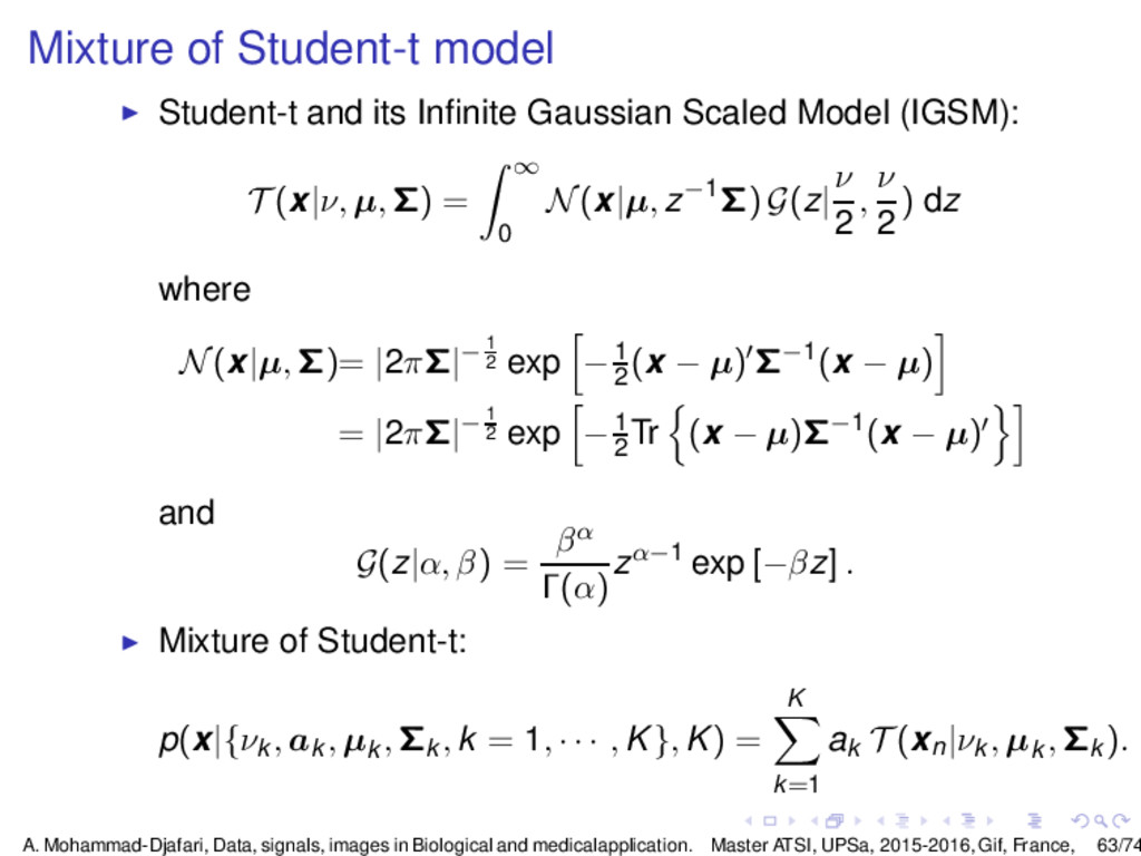
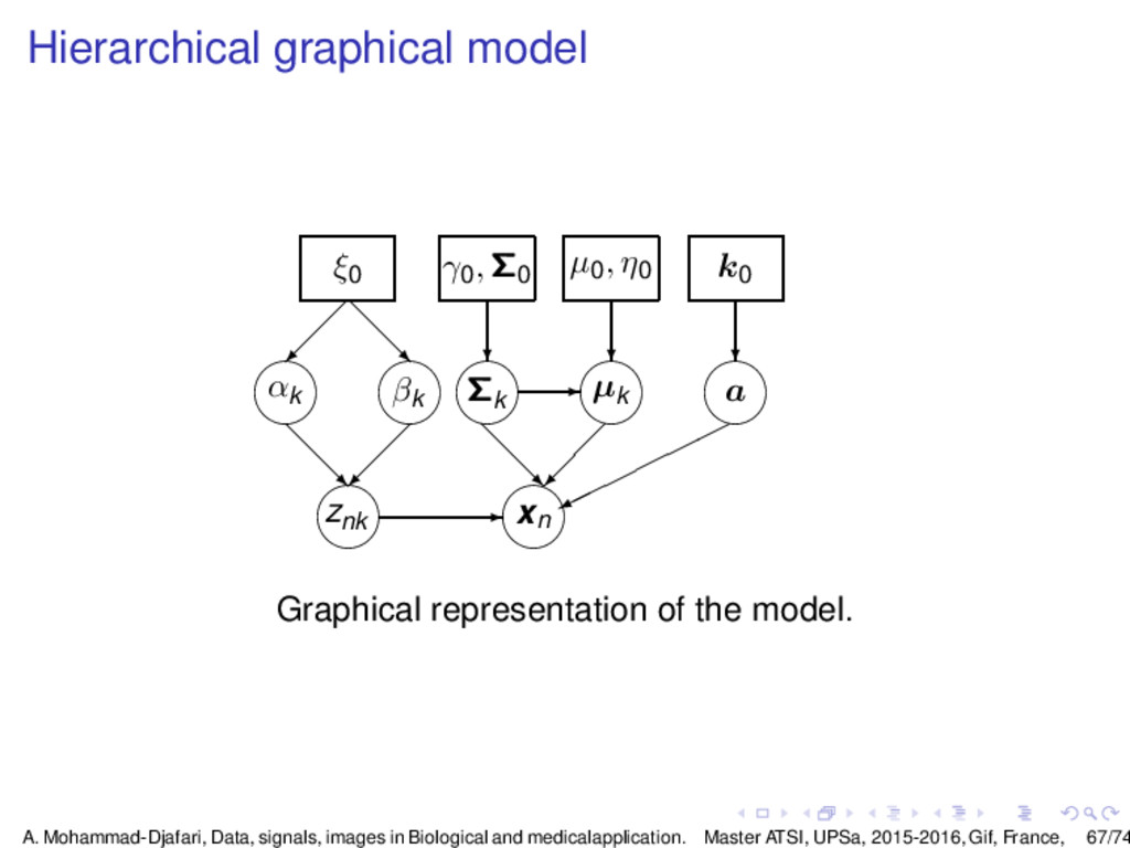
70. Proposed VBA for Mixture of Student-t priors model ◮ Using a generalized Student-t obtained by replacing G(zn,k |νk 2 , νk 2 ) by G(zn,k |αk , βk ) it will be easier to propose conjugate priors for αk , βk than for νk . p(xn, cn = k, znk |ak , µk , Σk , αk , βk , K) = ak N(xn |µk , z−1 n,k Σk ) G(zn,k |αk , βk ◮ In the following, noting by Θ = {(ak , µk , Σk , αk , βk ), k = 1, · · · , K}, we propose to use the factorized prior laws: p(Θ) = p(a) k [p(αk ) p(βk ) p(µk |Σk ) p(Σk )] with the following components:            p(a) = D(a|k0 ), k0 = [k0 , · · · , k0 ] = k0 1 p(αk ) = E(αk |ζ0 ) = G(αk |1, ζ0 ) p(βk ) = E(βk |ζ0 ) = G(αk |1, ζ0 ) p(µk |Σk ) = N(µk |µ01, η−1 0 Σk ) p(Σk ) = IW(Σk |γ0 , γ0 Σ0 ) A. Mohammad-Djafari, Data, signals, images in Biological and medicalapplication. Master ATSI, UPSa, 2015-2016, Gif, France, 70/74
71. Proposed VBA for Mixture of Student-t priors model where D(a|k) = Γ( l kk ) l Γ(kl ) l akl −1 l is the Dirichlet pdf, E(t|ζ0 ) = ζ0 exp [−ζ0t] is the Exponential pdf, G(t|a, b) = ba Γ(a) ta−1 exp [−bt] is the Gamma pdf and IW(Σ|γ, γ∆) = |1 2 ∆|γ/2 exp −1 2 Tr ∆Σ−1 ΓD (γ/2)|Σ|γ+D+1 2 . is the inverse Wishart pdf. With these prior laws and the likelihood: joint posterior law: pk (c, Z, Θ|X) = p(X, c, Z, Θ) p(X) . A. Mohammad-Djafari, Data, signals, images in Biological and medicalapplication. Master ATSI, UPSa, 2015-2016, Gif, France, 71/74
72. Expressions of q q(c, Z, Θ) = q(c, Z) q(Θ) = n k [q(cn = k|znk ) q(znk )] k [q(αk ) q(βk ) q(µk |Σk ) q(Σk )] q(a). with:                    q(a) = D(a|˜ k), ˜ k = [˜ k1 , · · · , ˜ kK ] q(αk ) = G(αk |˜ ζk , ˜ ηk ) q(βk ) = G(βk |˜ ζk , ˜ ηk ) q(µk |Σk ) = N(µk |µ, ˜ η−1Σk ) q(Σk ) = IW(Σk |˜ γ, ˜ γ ˜ Σ) With these choices, we have F(q(c, Z, Θ)) = ln p(X, c, Z, Θ|K) q(c,Z,Θ) = k n F1kn + k F2k F1kn = ln p(xn, cn, znk , θk ) q(cn=k|znk )q(znk ) F2k = ln p(xn, cn, znk , θk ) q(θk ) A. Mohammad-Djafari, Data, signals, images in Biological and medicalapplication. Master ATSI, UPSa, 2015-2016, Gif, France, 72/74
73. VBA Algorithm step Expressions of the updating expressions of the tilded parameters are obtained by following three steps: ◮ E step: Optimizing F with respect to q(c, Z) when keeping q(Θ) fixed, we obtain the expression of q(cn = k|znk ) = ˜ ak , q(znk ) = G(znk |αk , βk ). ◮ M step: Optimizing F with respect to q(Θ) when keeping q(c, Z) fixed, we obtain the expression of q(a) = D(a|˜ k), ˜ k = [˜ k1 , · · · , ˜ kK ], q(αk ) = G(αk |˜ ζk , ˜ ηk ), q(βk ) = G(βk |˜ ζk , ˜ ηk ), q(µk |Σk ) = N(µk |µ, ˜ η−1Σk ), and q(Σk ) = IW(Σk |˜ γ, ˜ γ ˜ Σ), which gives the updating algorithm for the corresponding tilded parameters. ◮ F evaluation: After each E step and M step, we can also evaluate the expression of F(q) which can be used for stopping rule of the iterative algorithm. ◮ Final value of F(q) for each value of K, noted Fk , can be used as a criterion for model selection, i.e.; the determination of the number of clusters. A. Mohammad-Djafari, Data, signals, images in Biological and medicalapplication. Master ATSI, UPSa, 2015-2016, Gif, France, 73/74
74. Conclusions ◮ Clustering and classification of a set of data are between the most important tasks in statistical researches for many applications such as data mining in biology. ◮ Mixture models and in particular Mixture of Gaussians are classical models for these tasks. ◮ We proposed to use a mixture of generalised Student-t distribution model for the data via a hierarchical graphical model. ◮ To obtain fast algorithms and be able to handle large data sets, we used conjugate priors everywhere it was possible. ◮ The proposed algorithm has been used for clustering, classification and discriminant analysis of some biological data (Cancer research related), but in this paper, we only presented the main algorithm. A. Mohammad-Djafari, Data, signals, images in Biological and medicalapplication. Master ATSI, UPSa, 2015-2016, Gif, France, 74/74