Master_ATSI_Univ_Paris_Sacly 2

Teaching Master courses at Univ. Paris Saclay
"Multi-componets Data, Signal and Image Processing for Biological and Medical Applications". Part 2

Transcript

1. . Multi-componets Data, Signal and Image Processing for Biological and Medical Applications Ali Mohammad-Djafari Laboratoire des Signaux et Syst` emes UMR 8506 CNRS - CS - Univ Paris Sud CentraleSup´ elec, Gif-sur-Yvette. djafari@lss.supelec.fr http://djafari.free.fr January 13, 2017 A. Mohammad-Djafari, Data, signals, images in Biological and medicalapplication. Master ATSI, UPSa, 2015-2016, Gif, France, 1/51
2. Summary 2.1: Time series ◮ Time serie and Fourier representation ◮ Continuous / Discrete ◮ Correlation, Inter-correlation, Inter-dependance ◮ Stationarity / non-stationarity ◮ Convolution and Deconvolution ◮ Filtering and Denoising ◮ Modelling and Prediction ◮ Parametric and Non parametric models ◮ Parametric models: ◮ Least Squares ◮ Maximum Likehood ◮ Bayesian estimation A. Mohammad-Djafari, Data, signals, images in Biological and medicalapplication. Master ATSI, UPSa, 2015-2016, Gif, France, 2/51
3. Summary 2.2: Images ◮ Continuous / Discrete ◮ Gray and Color images ◮ 2D FT and FFT ◮ 2D Correlation and inter-correlation ◮ Stationarity / non-stationarity ◮ 2D Convolution ◮ Filtering and Denoising ◮ Modelling and Prediction ◮ Simple Markovian models ◮ Contours and Regions ◮ Hierarchical Markov models A. Mohammad-Djafari, Data, signals, images in Biological and medicalapplication. Master ATSI, UPSa, 2015-2016, Gif, France, 3/51
4. 1D signals: Time series ◮ 1D Signal: Time series: xi = f(ti ) ◮ In general no exchangeable. ◮ Time representation f(t), Fourier Transform and Fourier representation F(ν), Auto Correlation function R(τ), Power Spectral Density S(ν) ◮ Stationary and non stationary ◮ STFT, Time-Frequency, Time-Scale, Wavelets, ... ◮ Smoothing, Noise removing, Filtering ◮ Periodic signals, estimation of the period, Fourier series ◮ Modeling: ◮ Sum of sinusoids model and parameter estimation ◮ Moving average (MA) model ◮ Autoregressive (AR) model A. Mohammad-Djafari, Data, signals, images in Biological and medicalapplication. Master ATSI, UPSa, 2015-2016, Gif, France, 4/51
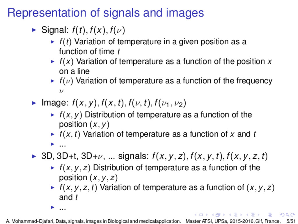
5. Representation of signals and images ◮ Signal: f(t), f(x), f(ν) ◮ f(t) Variation of temperature in a given position as a function of time t ◮ f(x) Variation of temperature as a function of the position x on a line ◮ f(ν) Variation of temperature as a function of the frequency ν ◮ Image: f(x, y), f(x, t), f(ν, t), f(ν1 , ν2 ) ◮ f(x, y) Distribution of temperature as a function of the position (x, y) ◮ f(x, t) Variation of temperature as a function of x and t ◮ ... ◮ 3D, 3D+t, 3D+ν, ... signals: f(x, y, z), f(x, y, t), f(x, y, z, t) ◮ f(x, y, z) Distribution of temperature as a function of the position (x, y, z) ◮ f(x, y, z, t) Variation of temperature as a function of (x, y, z) and t ◮ ... A. Mohammad-Djafari, Data, signals, images in Biological and medicalapplication. Master ATSI, UPSa, 2015-2016, Gif, France, 5/51
6. Representation of signals 0 10 20 30 40 50 60 70 80 90 100 -2.5 -2 -1.5 -1 -0.5 0 0.5 1 1.5 2 2.5 time Amplitude g(t) 1D signal 2D signal=image 3D signal A. Mohammad-Djafari, Data, signals, images in Biological and medicalapplication. Master ATSI, UPSa, 2015-2016, Gif, France, 6/51
7. Linear Transformations g(s) = D f(r) h(r, s) dr f(r) −→ h(r, s) −→ g(s) ◮ 1–D : g(t) = D f(t′) h(t, t′) dt′ g(x) = D f(x′) h(x, x′) dx′ ◮ 2–D : g(x, y) = D f(x′, y′) h(x, y; x′, y′) dx′ dy′ g(r, φ) = D f(x, y) h(x, y; r, φ) dx dy A. Mohammad-Djafari, Data, signals, images in Biological and medicalapplication. Master ATSI, UPSa, 2015-2016, Gif, France, 7/51
8. Linear and Invariant systems: convolution h(r, r′) = h(r − r′) f(r) −→ h(r) −→ g(r) = h(r) ∗ f(r) ◮ 1–D : g(t) = D f(t′) h(t − t′) dt′ g(x) = D f(x′) h(x − x′) dx′ ◮ 2–D : g(x, y) = D f(x, y) h(x − x′, y − y′) dx′ dy′ ◮ h(t) impulse response ◮ h(x, y) Point Spread Function A. Mohammad-Djafari, Data, signals, images in Biological and medicalapplication. Master ATSI, UPSa, 2015-2016, Gif, France, 8/51
9. Linear Transformations: Separable systems g(s) = D f(r) h(r, s) dr h(r, s) = j hj (rj , sj ) Examples: ◮ 2D Fourier Transform g(ωx, ωy ) = f(x, y) exp −j(ωxx + ωy y) dx dy h(x, y, ωx , ωy ) = h1 (ωx x) h2 (ωy y) exp −j(ωx x + ωyy) = exp [−j(ωxx)] exp −j(ωyy) ◮ nD Fourier Transform g(ω) = f(x) exp −jω′x) dx A. Mohammad-Djafari, Data, signals, images in Biological and medicalapplication. Master ATSI, UPSa, 2015-2016, Gif, France, 9/51
10. Fourier Transform [Joseph Fourier, French Mathematicien (1768-1830)] ◮ 1D Fourier: F1      g(ω) = f(t) exp [−jωt] dt f(t) = 1 2π g(ω) exp [+jωt] dω ◮ 2D Fourier: F2      g(ωx, ωy ) = f(x, y) exp −j(ωxx + ωyy dx dy f(x, y) = ( 1 2π )2 g(ωx, ωy ) exp +j(ωxx + ωy y dωx dωy ◮ nD Fourier: Fn      g(ω) = f(x) exp −jω′x dx f(x) = ( 1 2π )n g(ω) exp +jω′x dω A. Mohammad-Djafari, Data, signals, images in Biological and medicalapplication. Master ATSI, UPSa, 2015-2016, Gif, France, 10/51
11. 1D Fourier Transform F1      g(ω) = f(t) exp [−jωt] dt f(t) = 1 2π g(ω) exp [+jωt] dω ◮ |g(ω)|2 is called the spectrum of the signal f(t) ◮ For real valued signals f(t), |g(ω)| is symetric Examples: f(t) g(ω) exp [−jω0t] δ(ω − ω0 ) sin(ω0t) ? cos(ω0t) ? exp −t2 ? exp −1 2 (t − m)2/σ2 ? exp [−t/τ] , t > 0 ? 1 if |t| < T/2 ? A. Mohammad-Djafari, Data, signals, images in Biological and medicalapplication. Master ATSI, UPSa, 2015-2016, Gif, France, 11/51
12. 2D Fourier Transform: F2      g(ωx, ωy ) = f(x, y) exp −j(ωxx + ωy y dx dy f(x, y) = ( 1 2π )2 g(ωx, ωy ) exp +j(ωxx + ωyy dωx dωy ◮ |g(ωx, ωy )|2 is called the spectrum of the image f(x, y) ◮ For real valued image f(x, y), |g(ωx , ωy )| is symetric with respect of the two axis ωx and ωy . Examples: f(x, y) g(ωx, ωy ) exp −j(ωx0 x + ωy0 y) δ(ωx − ωx0 )δ(ωy − ωy0 ) exp −(x2 + y2) ? exp −1 2 [(x − mx)2/σ2 x + (y − my )2/σ2 y ] ? exp [−(|x| + |y|)] ? 1 if |x| < Tx/2 & |y| < Ty/2 ? 1 if (x2 + y2) < a ? A. Mohammad-Djafari, Data, signals, images in Biological and medicalapplication. Master ATSI, UPSa, 2015-2016, Gif, France, 12/51
13. nD Fourier Transform: Fn      g(ω) = f(x) exp −jω′x dx f(x) = ( 1 2π )n g(ω) exp +jω′x dω ◮ |g(ω)|2 is called the spectrum of f(x) ◮ For real valued image f(x), |g(ω)| is symetric with respect of all the axis ωj . Examples: f(x) g(ω) exp −j(ω′ 0x) δ(ω − ω0 ) exp [−x′x] = exp − x 2 exp [−ω′ω] = exp − ω 2 exp − Dx 2 ? exp −1 2 [(x − m)′Σ−1(x − m) ? 1 if x 2 < R ? 1 if |xj | < R ? A. Mohammad-Djafari, Data, signals, images in Biological and medicalapplication. Master ATSI, UPSa, 2015-2016, Gif, France, 13/51
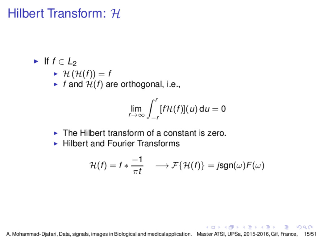
14. Hilbert Transform: H [David Hilbert, German mathematicien (1862-1943)] ◮ Definition: If f ∈ L2 on (−∞, ∞), g(x) = 1 π +∞ −∞ f(t) t − x dt f(t) = −1 π +∞ −∞ g(x) x − t dx The integrals are interpreted in the Cauchy principal value(CPV) sense at t = x. ◮ Alternate expression useful in signal processing: g(t) = 1 π lim ǫ→0 ∞ ǫ f(t + τ) − f(t − τ) τ dτ A. Mohammad-Djafari, Data, signals, images in Biological and medicalapplication. Master ATSI, UPSa, 2015-2016, Gif, France, 14/51
15. Hilbert Transform: H ◮ If f ∈ L2 ◮ H (H(f)) = f ◮ f and H(f) are orthogonal, i.e., lim r→∞ r −r [fH(f)](u) du = 0 ◮ The Hilbert transform of a constant is zero. ◮ Hilbert and Fourier Transforms H(f) = f ∗ −1 πt −→ F{H(f)} = jsgn(ω)F(ω) A. Mohammad-Djafari, Data, signals, images in Biological and medicalapplication. Master ATSI, UPSa, 2015-2016, Gif, France, 15/51
16. Radon Transform (RT): R ◮ Definition: This transform is defined for the functions in 2 or more dimensions. Here we give the relations only in the 2–D case. g(r, φ) = Lr,φ f(x, y) dl = f(x, y) δ(r − x cos(φ) − y sin(φ)) dx dy ◮ The Radon transform maps the spatial domain (x, y) ∈ I R2 to the domain (r, φ) ∈ I R × [0, π]. Each point in the (r, φ) space corresponds to a line in the spatial domain (x, y). ◮ Note that (r, φ) are not the polar coordinates of (x, y). In fact if we note the polar coordinates corresponding to the (x, y) point (ρ, θ), then we have x = ρ cos θ, y = ρ sin θ, r = ρ cos(φ − θ) A. Mohammad-Djafari, Data, signals, images in Biological and medicalapplication. Master ATSI, UPSa, 2015-2016, Gif, France, 16/51
17. X ray Tomography f(x, y) ✲ x ✻ y ✁ ✁ ✁ ❅ ❅ ❅ ❅ ❅ ❍ ❍ ❍ ✒ r φ •D g(r, φ) S• ❅ ❅ ❅ ❅ ❅ ❅ ❅ ❅ ❅ ❅ ❅ ❅ ✁ ✁ I = I0 exp − L f(x) dx − ln I I0 = L f(x, y) dl g(r, φ) = L f(x, y) dl g(r, φ) = L f(x, y) dl = f(x, y)δ(r − x cos φ − y sin φ) dx dy f(x, y) −→ Radon Transform −→ g(r, φ) g(r, φ) −→ Image Reconstruction −→ f(x, y) A. Mohammad-Djafari, Data, signals, images in Biological and medicalapplication. Master ATSI, UPSa, 2015-2016, Gif, France, 17/51
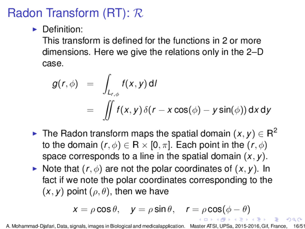
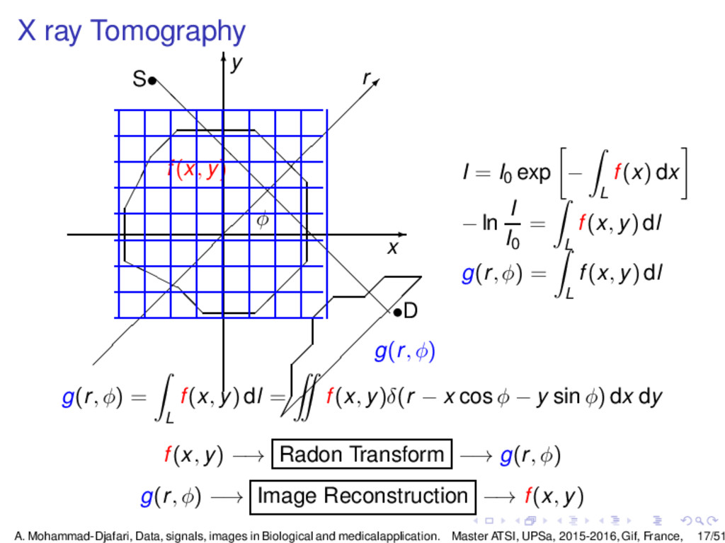
18. Radon Transform: Some properties [Johann K.A. Radon, Austrian mathematician (1887-1956)] ◮ Definition in cartezian coordinate system: f(x, y) = R −→ g(r, φ) = f(x, y)δ(r−x cos(φ)−y sin(φ)) dx dy ◮ Definition in polar coordinate system: f(ρ, θ) R −→ g(r, φ) = ∞ 0 2π 0 f(ρ, θ)δ(r −ρ cos(φ−θ)ρ dρ dθ ◮ Inversion f(x, y) = 1 2π π 0 ∞ 0 ∂g(r, φ)/∂r r − x cos(φ) − y sin(φ) dr dφ A. Mohammad-Djafari, Data, signals, images in Biological and medicalapplication. Master ATSI, UPSa, 2015-2016, Gif, France, 18/51
19. Radon Transform: Inversion Direct Inverse Radon Transform g(r,φ) −→ Differentiate 1 2π D −→ Hilbert Transform H g(r,φ) −→ Back–projection B f(x,y −→ Convolution Back–projection method g(r,φ) −→ 1–D Filter |Ω| g(r,φ) −→ Back–projection B f(x,y) −→ Filter Back–projection method g(r,φ) −→ FT F1 −→ Filter Ω −→ IFT F−1 1 g(r,φ) −→ Back–projection B f(x,y) −→ A. Mohammad-Djafari, Data, signals, images in Biological and medicalapplication. Master ATSI, UPSa, 2015-2016, Gif, France, 19/51
20. Radon Transform (RT) and Filtered Back-Projection (FBP) image reconstruction f(x,y) -3 -2 -1 0 1 2 3 x -250 -200 -150 -100 -50 0 50 100 150 200 250 y 0 0.2 0.4 0.6 0.8 1 1.2 1.4 1.6 1.8 2 g(r, φ) -300 -200 -100 0 100 200 300 r 0 20 40 60 80 100 120 140 160 φ in degrees 0 50 100 150 200 250 300 350 fh(x,y) -200 -100 0 100 200 x -250 -200 -150 -100 -50 0 50 100 150 200 250 y 0 0.2 0.4 0.6 0.8 1 1.2 1.4 1.6 1.8 2 a) original f(x, y) b) RT g(r, φ) c) FBP reconstruction f(x, y) A. Mohammad-Djafari, Data, signals, images in Biological and medicalapplication. Master ATSI, UPSa, 2015-2016, Gif, France, 20/51
21. Radon Transform (RT), Back-Projection (BP) and Filtered Back-Projection (FBP) image reconstruction f(x,y) -3 -2 -1 0 1 2 3 x -250 -200 -150 -100 -50 0 50 100 150 200 250 y 0 0.2 0.4 0.6 0.8 1 1.2 1.4 1.6 1.8 2 x y fhBP(x,y) -3 -2 -1 0 1 2 3 -250 -200 -150 -100 -50 0 50 100 150 200 250 0 0.2 0.4 0.6 0.8 1 1.2 1.4 1.6 1.8 2 fhFBP(x,y) -3 -2 -1 0 1 2 3 x -250 -200 -150 -100 -50 0 50 100 150 200 250 y 0 0.2 0.4 0.6 0.8 1 1.2 1.4 1.6 1.8 2 a) f(x, y) b) f(x, y) by BP f(x, y) by FBP g(r, φ) -300 -200 -100 0 100 200 300 r 0 20 40 60 80 100 120 140 160 φ in degrees 0 50 100 150 200 250 300 350 x y ghBP(r,φ) -300 -200 -100 0 100 200 300 0 20 40 60 80 100 120 140 160 0 50 100 150 200 250 300 350 ghFBP(r, φ) -300 -200 -100 0 100 200 300 r 0 20 40 60 80 100 120 140 160 φ in degrees 0 50 100 150 200 250 300 350 A. Mohammad-Djafari, Data, signals, images in Biological and medicalapplication. Master ATSI, UPSa, 2015-2016, Gif, France, 21/51
22. 1D signals f(t) and its FT F(ν) 0 10 20 30 40 50 60 70 80 90 -2 -1.5 -1 -0.5 0 0.5 1 1.5 2 time Amplitude g(t) 47 24 16 12 9 8 0 0.1 0.2 0.3 0.4 0.5 0.6 0.7 0.8 0.9 1 periods Amplitude FFT 0 10 20 30 40 50 60 70 80 90 -2 -1.5 -1 -0.5 0 0.5 1 1.5 2 time Amplitude g(t) 47 24 16 12 9 8 0 0.1 0.2 0.3 0.4 0.5 0.6 0.7 0.8 0.9 1 periods Amplitude FFT 0 10 20 30 40 50 60 70 80 90 -2 -1.5 -1 -0.5 0 0.5 1 1.5 2 time Amplitude g(t) 95 32 19 14 11 9 0 0.1 0.2 0.3 0.4 0.5 0.6 0.7 0.8 0.9 1 periods Amplitude FFT signal f(t) Modulus of its FT |F(ν)|2 A. Mohammad-Djafari, Data, signals, images in Biological and medicalapplication. Master ATSI, UPSa, 2015-2016, Gif, France, 22/51
23. 1D signals: Noise removing using FT g(t) = f(t) + ǫ(t) g(t) −→ FFT −→ Threshold −→ IFFT −→ f(t) g(t) = f(t) + ǫ(t) →FFT→ G(ω) = F(ω) + E(ω) t 0 50 100 150 200 250 300 350 400 450 500 -1.5 -1 -0.5 0 0.5 1 1.5 f(t) g(t) 1/T0 0 0.1 0.2 0.3 0.4 0.5 0.6 G(ω) f ←IFFT← Thresholded G(ω) t 0 50 100 150 200 250 300 350 400 450 500 -1.5 -1 -0.5 0 0.5 1 1.5 f(t) fh(t) ω 1/T0 0 0.1 0.2 0.3 0.4 0.5 0.6 G(ω) A. Mohammad-Djafari, Data, signals, images in Biological and medicalapplication. Master ATSI, UPSa, 2015-2016, Gif, France, 23/51
24. 1D signals: Noise removing using FT g(t) = f(t) + ǫ(t) →FFT→ G(ω) = F(ω) + E(ω) t 0 50 100 150 200 250 300 350 400 450 500 -1.5 -1 -0.5 0 0.5 1 1.5 f(t) g(t) 1/T0 0 0.1 0.2 0.3 0.4 0.5 G(ω) f ←IFFT← Thresholded G(ω) t 0 50 100 150 200 250 300 350 400 450 500 -1.5 -1 -0.5 0 0.5 1 1.5 f(t) fh(t) ω 1/T0 0 0.1 0.2 0.3 0.4 0.5 G(ω) A. Mohammad-Djafari, Data, signals, images in Biological and medicalapplication. Master ATSI, UPSa, 2015-2016, Gif, France, 24/51
25. 1D signals: Noise removing using FT g(t) = f(t) + ǫ(t) →FFT→ G(ω) = F(ω) + E(ω) t 0 50 100 150 200 250 300 350 400 450 500 -1.5 -1 -0.5 0 0.5 1 1.5 f(t) g(t) 1/T0 0 0.05 0.1 0.15 0.2 0.25 0.3 0.35 0.4 G(ω) f ←IFFT← Thresholded G(ω) t 0 50 100 150 200 250 300 350 400 450 500 -1.5 -1 -0.5 0 0.5 1 1.5 f(t) fh(t) ω 1/T0 0 0.05 0.1 0.15 0.2 0.25 0.3 0.35 0.4 G(ω) A. Mohammad-Djafari, Data, signals, images in Biological and medicalapplication. Master ATSI, UPSa, 2015-2016, Gif, France, 25/51
26. Images denoising using FFT 0 0.1 0.2 0.3 0.4 0.5 0.6 0.7 0.8 0.9 1 -0.2 0 0.2 0.4 0.6 0.8 1 1.2 0 1 2 3 4 5 6 7 8 f(x, y) g(x, y) = f(x, y) + ǫ(x, y) F(u, v) -0.2 0 0.2 0.4 0.6 0.8 1 1.2 0 1 2 3 4 5 6 7 8 1 2 3 4 5 6 7 8 f(x, y) Thresholded G(u, v) G(u, v) A. Mohammad-Djafari, Data, signals, images in Biological and medicalapplication. Master ATSI, UPSa, 2015-2016, Gif, France, 26/51
27. Images: Pyramidal and Wavelet Transform Pyramidal representation: ◮ Invertible Linear Transform ◮ image −→ Coarse and Fine images ◮ B: Band Pass Filtering Recon ✲ ✲ ✻ ✻ B ✲ Coarse Fine ✲ ❄ ❄ -❦ + ❦ ✲ ✻ B ✲ B❄ Input ✲ ◮ Number of samples: (1 + 1/2 + 1/4 + ...) ◮ Overcomplete representation A. Mohammad-Djafari, Data, signals, images in Biological and medicalapplication. Master ATSI, UPSa, 2015-2016, Gif, France, 27/51
28. Images: Pyramidal representations 0 50 100 150 200 Original Pyramid Pyramid A. Mohammad-Djafari, Data, signals, images in Biological and medicalapplication. Master ATSI, UPSa, 2015-2016, Gif, France, 28/51
29. Images: QMF and Wavelet Transform ◮ Invertible Linear Transform ◮ image −→ Coarse and Fine images ◮ Quadrature Mirror Filtering HF❄ ✻ HF ✲ LF ✻ Recon ✲ ✲ ✻ ✲ + ♥ ✲ ✲ LF ❄ Coarse Fine ✲ Input ✲ ◮ Number of samples: 1 ◮ Complete representation A. Mohammad-Djafari, Data, signals, images in Biological and medicalapplication. Master ATSI, UPSa, 2015-2016, Gif, France, 29/51
30. Images: Pyramidal representations 0 50 100 150 200 Original Pyramid Pyramid 0 0.5 1 1.5 2 2.5 3 3.5 4 4.5 5 0 0.5 1 1.5 2 2.5 3 3.5 4 4.5 5 0 0.5 1 1.5 2 2.5 3 3.5 4 4.5 5 WT 1 WT 2 WT 3 A. Mohammad-Djafari, Data, signals, images in Biological and medicalapplication. Master ATSI, UPSa, 2015-2016, Gif, France, 30/51
31. Images compression using WT 0 0.1 0.2 0.3 0.4 0.5 0.6 0.7 0.8 0.9 1 0 0.1 0.2 0.3 0.4 0.5 0.6 0 0.1 0.2 0.3 0.4 0.5 0.6 Original WT 1 WT 2 0 0.1 0.2 0.3 0.4 0.5 0.6 0 0.2 0.4 0.6 0.8 1 0 0.2 0.4 0.6 0.8 1 1.2 WT 1-2 IWT 1-1 IWT 1-2 A. Mohammad-Djafari, Data, signals, images in Biological and medicalapplication. Master ATSI, UPSa, 2015-2016, Gif, France, 31/51
32. Images compression using WT 0 50 100 150 200 0 0.5 1 1.5 2 2.5 3 3.5 4 4.5 5 0 0.5 1 1.5 2 2.5 3 3.5 4 4.5 5 Original WT 1 WT 2 0 0.5 1 1.5 2 2.5 3 3.5 4 4.5 5 40 60 80 100 120 140 160 180 200 220 40 60 80 100 120 140 160 180 200 220 240 WT 1-2 IWT 1-1 IWT 1-2 A. Mohammad-Djafari, Data, signals, images in Biological and medicalapplication. Master ATSI, UPSa, 2015-2016, Gif, France, 32/51
33. Images: Different representations 0 50 100 150 200 4 6 8 10 12 14 0 0.5 1 1.5 2 2.5 3 3.5 4 4.5 5 Original FFT WT 2 Pyramid Pyramid Laplacien A. Mohammad-Djafari, Data, signals, images in Biological and medicalapplication. Master ATSI, UPSa, 2015-2016, Gif, France, 33/51
34. Images: Space, Fourier and Wavelets representations 50 100 150 200 250 50 100 150 200 250 50 100 150 200 250 50 100 150 200 250 A. Mohammad-Djafari, Data, signals, images in Biological and medicalapplication. Master ATSI, UPSa, 2015-2016, Gif, France, 34/51
35. Sparse images (Fourier and Wavelets domain) Image Fourier Wavelets 0 50 100 150 200 250 0 500 1000 1500 2000 2500 3000 3500 0 2 4 6 8 10 12 14 16 0 1000 2000 3000 4000 5000 6000 -500 -400 -300 -200 -100 0 100 200 300 400 500 0 2 4 6 8 10 Image hist. Fourier coeff. hist. Wavelet coeff. hist. -200 -150 -100 -50 0 50 100 150 200 0 1000 2000 3000 4000 5000 6000 7000 8000 -200 -150 -100 -50 0 50 100 150 200 0 200 400 600 800 1000 1200 1400 -200 -150 -100 -50 0 50 100 150 200 0 50 100 150 200 250 300 350 400 450 bands 1-3 bands 4-6 bands 7-9 A. Mohammad-Djafari, Data, signals, images in Biological and medicalapplication. Master ATSI, UPSa, 2015-2016, Gif, France, 35/51
36. Temperature and activity Time series before, during and some treatment 0 24 48 30 32 34 36 38 BOD: before Temperature 0 24 48 0 200 400 600 800 Activity 0 24 48 30 32 34 36 38 BOD: during Temperature 0 24 48 0 200 400 600 800 Activity 0 24 48 30 32 34 36 38 BOD: after Temperature 0 24 48 0 200 400 600 800 Activity A. Mohammad-Djafari, Data, signals, images in Biological and medicalapplication. Master ATSI, UPSa, 2015-2016, Gif, France, 36/51
37. A. Mohammad-Djafari, Data, signals, images in Biological and medicalapplication. Master ATSI, UPSa, 2015-2016, Gif, France, 37/51
38. Simple questions for 1D time series ◮ Main question: Has something changed during and some medical action? ◮ In this study: effects of circadian cycle on cancer cells. 1. Is there any periodic components in these signals? Yes/No (Detection)? Confidence ? 2. If Yes, How many? 3. What are those components (Periods pi or Frequencies νi , Amplitudes ai )? ◮ When questions 1 and 2 are answered, the problem becomes easier: Parameter estimation ◮ Trying to answer all the three questions at the same time: semi- or Non-Parametric modelling ◮ Biologists always need uncertainties −→ Bayesian inference A. Mohammad-Djafari, Data, signals, images in Biological and medicalapplication. Master ATSI, UPSa, 2015-2016, Gif, France, 38/51
39. Simple Analysis tools may not be successful even in very simple cases Case of 1 sinusoid 0 24 48 72 -1 -0.8 -0.6 -0.4 -0.2 0 0.2 0.4 0.6 0.8 1 time (hours) 24 0 0.1 0.2 0.3 0.4 0.5 0.6 0.7 period in hours Case of 2 sinusoids+noise 0 24 48 72 -1 -0.8 -0.6 -0.4 -0.2 0 0.2 0.4 0.6 0.8 1 time (hours) 24 12 0 0.1 0.2 0.3 0.4 0.5 0.6 0.7 period in hours Case of 3 sinusoids+noise 0 24 48 72 -1 -0.8 -0.6 -0.4 -0.2 0 0.2 0.4 0.6 0.8 1 time (hours) Inf 36 24 14.4 0 0.05 0.1 0.15 0.2 0.25 0.3 0.35 0.4 0.45 period in hours A. Mohammad-Djafari, Data, signals, images in Biological and medicalapplication. Master ATSI, UPSa, 2015-2016, Gif, France, 39/51
40. Classical methods: Spectral estimation S(ω) ? ◮ Fast Fourier Transform (FFT): g(t) −→ FFT −→ f(ω) −→ S(ω) = |f(ω)|2 ◮ Advantages: Well-known and understood, fast ◮ Drawbacks: linear in frequencies ν, but not equidistance in periods ν = [0, · · · , N − 1] −→ p = [∞, 1, · · · , 1/(N − 1)] ◮ Autocorrelation function: γ(τ) ◮ If g(t) is periodic, then γ(τ) is also periodic, but much smoother ◮ γ(0) = 1 γ(τ) ≤ γ(0), ∀τ ◮ Power spectral density: γ(τ) −→ FFT −→ S(ω) ◮ Autoregressive (AR), Moving Average (MA) and ARMA models ◮ Non-stationary GARCH models ◮ Sum of sinusoidal components A. Mohammad-Djafari, Data, signals, images in Biological and medicalapplication. Master ATSI, UPSa, 2015-2016, Gif, France, 40/51
41. Parametric, Semi- and Non-Parametric models ◮ Parametric: g(t) = K k=1 ak sin(2πνk t + φk ) + ǫ(t), θ = {ak , φk , νk } g(t) = K k=1 ak cos(2πνk t)+bk sin(2πνk t)+ǫ(t), θ = {ak , bk , νk } g(t) = K k=1 ck exp [j2πνk t]+ǫ(t), θ = {ck , νk }, t = 0, · · · , T ◮ Semi-Parametric: νk = kν0 , ν0 = 1/T, K = T −→ DFT ◮ Non-Parametric: νk fixed in a given interval with given precision, so K is fixed but can be as large as necessary. g(t) = K k=1 ck exp [j2πνk t] + ǫ(t), θ = {ck } Linear model A. Mohammad-Djafari, Data, signals, images in Biological and medicalapplication. Master ATSI, UPSa, 2015-2016, Gif, France, 41/51
42. Can we propose a unifying approach for all these problems? My answer is Yes: ◮ Identify what your are looking for. (red color f) ◮ Identify what are the data : (blue color g) ◮ Consider the errors (modeling and measurement ǫ) ◮ Write the Forward model relating them: g = Hf + ǫ ◮ Write the expression of the likelihood p(g|f) ◮ Translate your prior knowledge on the unknowns in p(f) ◮ Use the Bayes rule: p(f|g) = p(g|f) p(f) p(g) ∝ p(g|f) p(f) ◮ Infer on f using the posterior p(f|g): ◮ Maximum A Posteriori (MAP): f = arg max f {p(f|g)} ◮ Posterior Mean (PM): f = f p(f|g) df A. Mohammad-Djafari, Data, signals, images in Biological and medicalapplication. Master ATSI, UPSa, 2015-2016, Gif, France, 42/51
43. Estimating Periodic Components: Inverse Problems Approach g(t) = K k=1 ck exp [j2πνk t] + ǫ(t), θ = {ck } Linear model Slight changes of notations: use of periods pn in place of frequencies νk and fn in place of ck : g(t) = N n=1 fn exp [j2π/pmt] + ǫ(t), t = m∆t, m = 1, · · · , M Defining the vectors: g = [g1 , · · · , gM ]′, ǫ = [ǫ1 , · · · , ǫM ]′, f = [f1 , · · · , fN ]′ and the matrix H: Hm,n = exp [j2π/pmm∆t], we obtain: g = Hf + ǫ The objective is to infer on f. A. Mohammad-Djafari, Data, signals, images in Biological and medicalapplication. Master ATSI, UPSa, 2015-2016, Gif, France, 43/51
44. Inverse Problems Approach g = Hf + ǫ Bayesian approach: ◮ Assign the Likelihood : p(g|f) ◮ Assign the prior law: p(f) ◮ Use the Bayes rule : p(f|g) ∝ p(g|f) p(f) ◮ MAP: f = arg max f {p(f|g)} = arg min f {J(f)} ◮ Assuming Gaussian noise and Gaussian prior p(f|g) = N(f|f, Σ) with Σ = (H′H+λI)−1 and f = arg max f {J(f)} J(f) = g − Hf 2 + λ f 2 ◮ Other priors (Generalized Gaussian, Student-t or Cauchy) J(f) = g − Hf 2 + λΩ(f) A. Mohammad-Djafari, Data, signals, images in Biological and medicalapplication. Master ATSI, UPSa, 2015-2016, Gif, France, 44/51
45. Bayesian estimation with priors enforcing sparsity ◮ Sparsity: For any periodic signal, the spectrum is a set of Diracs ◮ Biological signals related to clock genes: a few independent oscillators ◮ Spectrum has a few non zero elements in any given interval g(m∆t) = N n=1 fn exp [−j2π/pm m∆t] + ǫ(t), m = 1, · · · , M g = Hf + ǫ with f sparse ◮ The question is now: How to translate sparsity? ◮ Two solutions: L1 regularization and Bayesian sparsity enforcing priors. ◮ Three main options in Bayesian: Genealized Gaussian, Student-t, mixtures models A. Mohammad-Djafari, Data, signals, images in Biological and medicalapplication. Master ATSI, UPSa, 2015-2016, Gif, France, 45/51
46. Bayesian estimation with priors enforcing sparsity ◮ g = Hf + ǫ with f sparse ◮ To translate this information use the heavy tailed prior law Student-t with its hierarchical structure and hidden variables St(fj |ν) ∝ exp − ν + 1 2 log 1 + f2 j /ν ◮ Infinite Gaussian Scaled Mixture (IGSM) property: St(f j |ν) ∝= ∞ 0 N(fj |, 0, 1/zj ) G(zj |α, β) dzj , with α = β = ν/2 ◮ Hiearchical prior model: p(fj |zj ) = N(fj |0, 1/zj ), p(zj ) = G(zj |α, β)    p(f|z) = j p(fj |zj ) p(z) = j p(zj ) −→ p(g|f) = N(g|Hf, σ2 ǫ I) p(f, z|g) ∝ p(g|f)p(f|z)p(z) A. Mohammad-Djafari, Data, signals, images in Biological and medicalapplication. Master ATSI, UPSa, 2015-2016, Gif, France, 46/51
47. Results on simulated and real activity data Number of days 0 1 2 Amplitude -4 -2 0 2 4 6 8 10 CT 502 B3 Activity DDBef Signal CT 502 B3 Activity DDBef Signal Periods 8 9 10 11 12 13 14 15 16 17 18 19 20 21 22 23 24 25 26 27 28 29 30 31 32 Amplitude 0 0.2 0.4 0.6 0.8 1 1.2 1.4 1.6 1.8 2 CT 502 B3 Activity DDBef VBA Periods 6 6.54 7.2 8 9 10.28 12 14.4 18 24 36 Amplitude 0 0.2 0.4 0.6 0.8 1 1.2 1.4 1.6 1.8 2 fF F T CT 502 B3 Activity DDBef FFT Data BEFORE Proposed method FFT Number of days 0 1 2 3 4 Amplitude -2 0 2 4 6 8 10 CT 502 B3 Activity DDDur Signal CT 502 B3 Activity DDDur Signal Periods 8 9 10 11 12 13 14 15 16 17 18 19 20 21 22 23 24 25 26 27 28 29 30 31 32 Amplitude 0 0.2 0.4 0.6 0.8 1 1.2 1.4 CT 502 B3 Activity DDDur VBA Periods 8 8.57 9.23 10 10.9 12 13.33 15 17.14 20 24 30 Amplitude 0 0.2 0.4 0.6 0.8 1 1.2 1.4 fF F T CT 502 B3 Activity DDDur FFT Data DURING Proposed method FFT Number of days 0 1 Amplitude -2 0 2 4 6 8 10 CT 502 B3 Activity DDAft Signal CT 502 B3 Activity DDAft Signal Periods 8 9 10 11 12 13 14 15 16 17 18 19 20 21 22 23 24 25 26 27 28 29 30 31 32 Amplitude 0 0.2 0.4 0.6 0.8 1 1.2 1.4 1.6 1.8 2 CT 502 B3 Activity DDAft VBA Periods 6 6.85 8 9.6 12 16 24 48 Amplitude 0 0.2 0.4 0.6 0.8 1 1.2 1.4 1.6 1.8 2 fF F T CT 502 B3 Activity DDAft FFT Data AFTER Proposed method FFT A. Mohammad-Djafari, Data, signals, images in Biological and medicalapplication. Master ATSI, UPSa, 2015-2016, Gif, France, 47/51
48. Computed Tomography as Linear Inverse Problem f all the pixels of the object put together in a vector; g all the projection data put together in a vector; gk the projection at angle φk , so that g = [g1 ; g2 ; · · · , gK ]; H the forward problem matrix: Hi,j is the length of the ray i in the pixel j; Hk the forward problem matrix for the projection at angle φk , so that H = [H1 ; H2 ; · · · , HK ]; ǫ the noise over all the projection data; ǫk the noise over the projection at angle φk so that ǫ = [ǫ1 ; ǫ2 ; · · · , ǫK ]. gk = Hk f + ǫk −→ g = Hf + ǫ with Ht = [Ht 1 , · · · , Ht K ], gt = [gt 1 , · · · , gt K ], ǫt = [ǫt 1 , · · · , ǫt K ], where K is the number of projections at angles φ = [φ1 , · · · , φK ]. A. Mohammad-Djafari, Data, signals, images in Biological and medicalapplication. Master ATSI, UPSa, 2015-2016, Gif, France, 48/51
49. Computed Tomography: BP and FBP Back-Projection (BP) f = Ht g = K k=1 Ht k gk . Filtered Back-Projection (FBP) f = Ht g = K k=1 Ht k gk . where gk is the |Ω| filtered of gk . It can also be regarded as the minimum norm solution of Hf = g: minimize f 2 2 subject to Hf = g f = Ht (HHt )−1g = K k=1 Ht k (Hk Ht k )−1gk . A. Mohammad-Djafari, Data, signals, images in Biological and medicalapplication. Master ATSI, UPSa, 2015-2016, Gif, France, 49/51
50. Computed Tomography: LS and Regularization Least-Square (LS) and Quadratic Regularization (QR) methods f = arg min f {J(f)} with J(f) = g − Hf 2 2 + λ Df 2 2 which is given by f = (Ht H + λDt D)−1Ht g. J(f) = K k=1 gk − Hk f 2 2 + λ Df 2 2 f = K k=1 (Ht k Hk + λDt D)−1Ht k g. A. Mohammad-Djafari, Data, signals, images in Biological and medicalapplication. Master ATSI, UPSa, 2015-2016, Gif, France, 50/51
51. Computed Tomography: Images, Contours, Regions f(x,y) -3 -2 -1 0 1 2 3 x -250 -200 -150 -100 -50 0 50 100 150 200 250 y 0 0.2 0.4 0.6 0.8 1 1.2 1.4 1.6 1.8 2 z(x,y) -200 -100 0 100 200 x -250 -200 -150 -100 -50 0 50 100 150 200 250 y 0 1 2 3 4 5 6 7 8 9 q(x,y) 50 100 150 200 250 300 350 400 450 500 x 50 100 150 200 250 300 350 400 450 500 y 0 0.1 0.2 0.3 0.4 0.5 0.6 0.7 0.8 0.9 1 f(x, y) z(x, y) q(x, y) Next week: Markovian and Hierarchical models A. Mohammad-Djafari, Data, signals, images in Biological and medicalapplication. Master ATSI, UPSa, 2015-2016, Gif, France, 51/51