Master_ATSI_Univ_Paris_Sacly 1

Teaching Master courses at Univ. Paris Saclay
"Multi-componets Data, Signal and Image Processing for Biological and Medical Applications". Part1
Applications

Transcript

1. . Multi-componets Data, Signal and Image Processing for Biological and Medical Applications Ali Mohammad-Djafari Laboratoire des Signaux et Syst` emes UMR 8506 CNRS - CS - Univ Paris Sud CentraleSup´ elec, Gif-sur-Yvette. djafari@lss.supelec.fr http://djafari.free.fr January 6, 2017 A. Mohammad-Djafari, Data, signals, images in Biological and medicalapplication. Master ATSI, UPSa, 2015-2016, Gif, France, 1/56
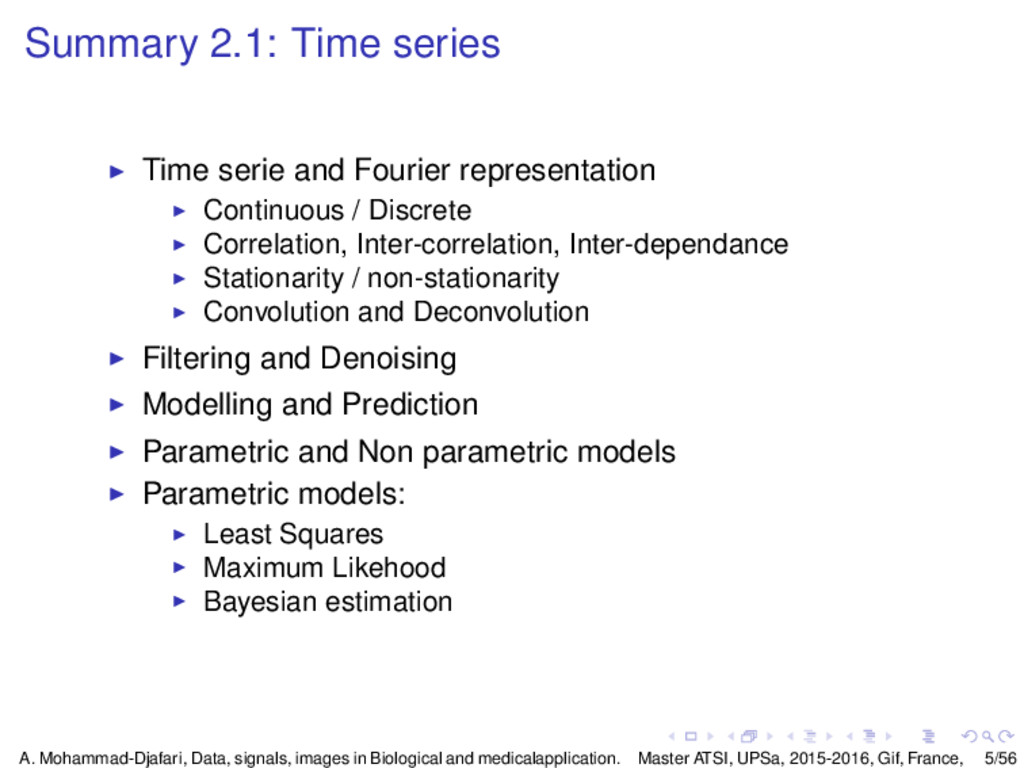
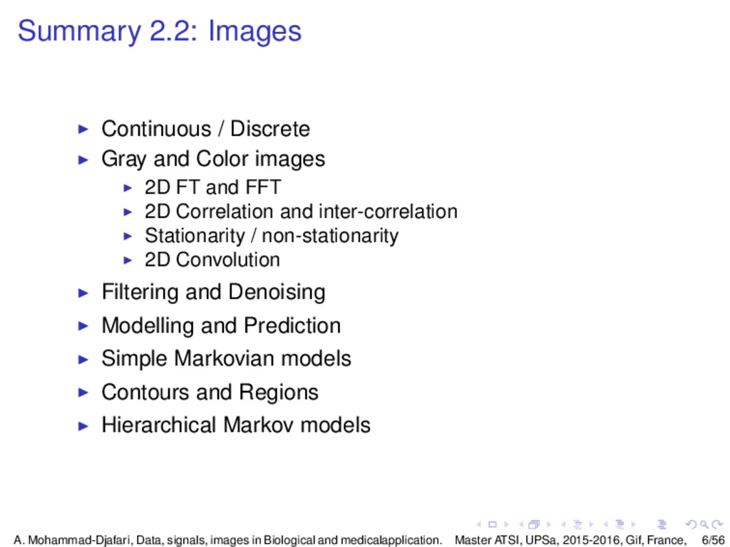
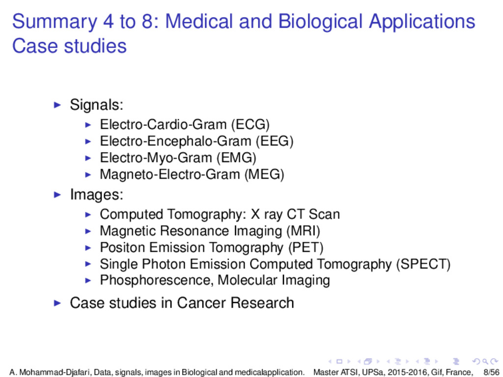
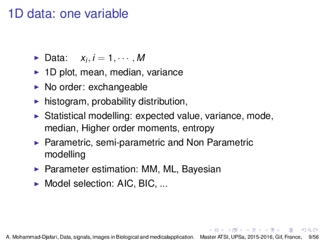
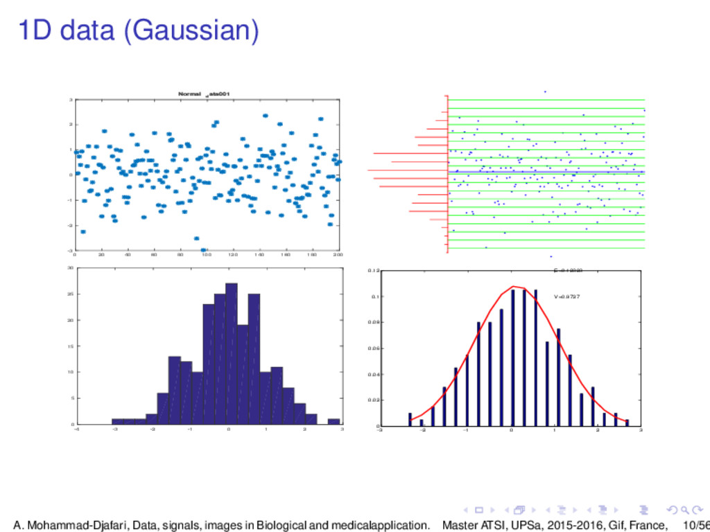
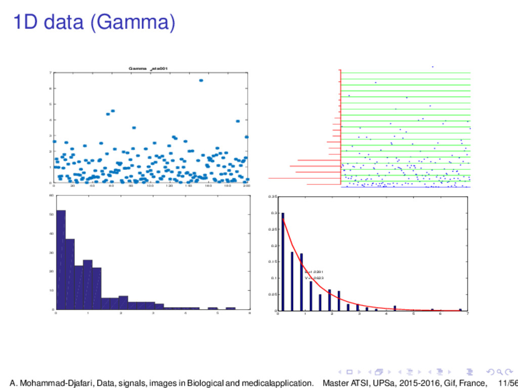
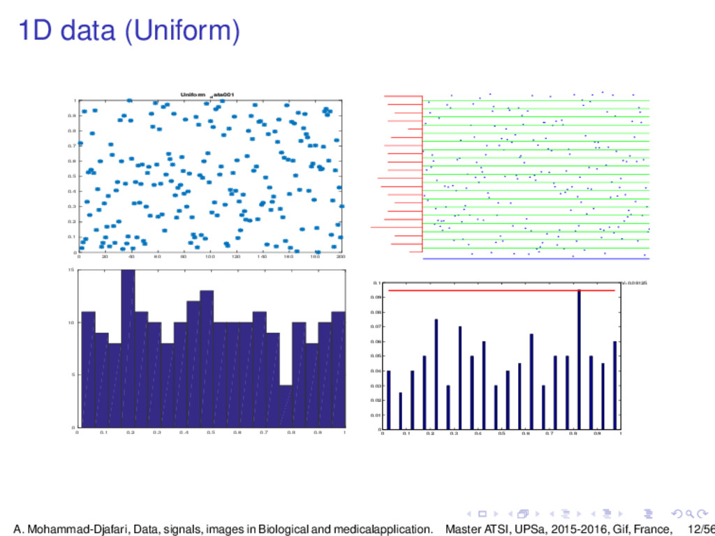
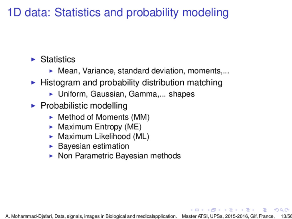
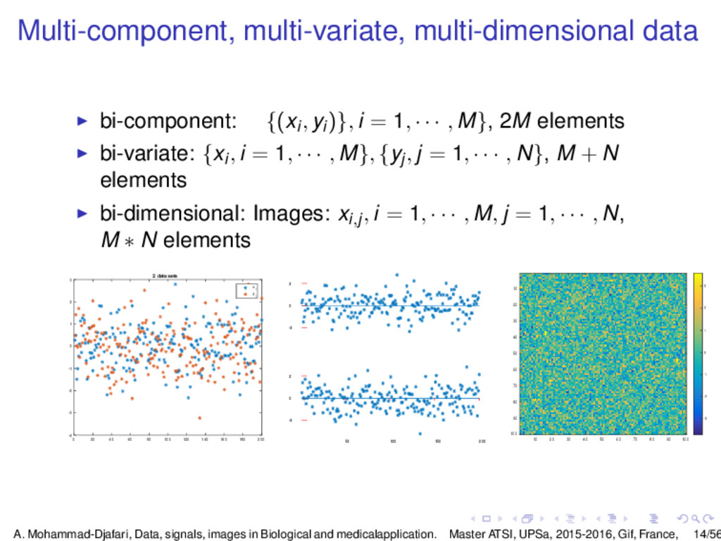
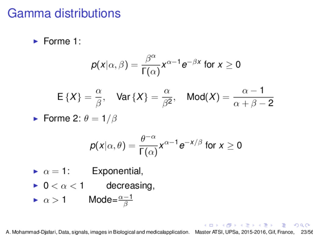
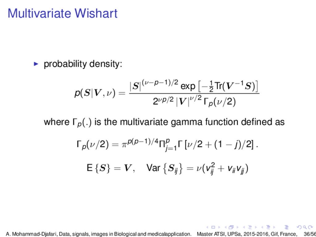
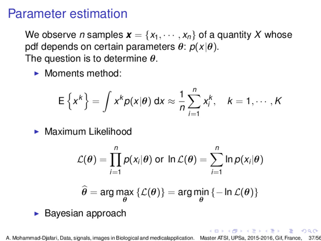
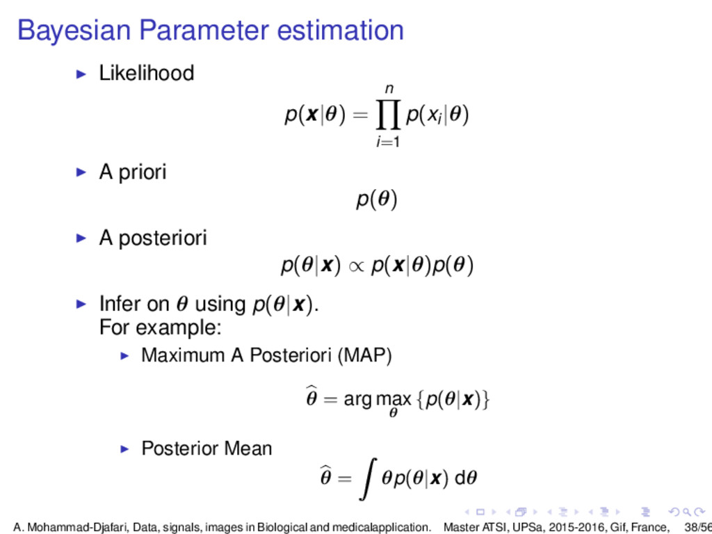
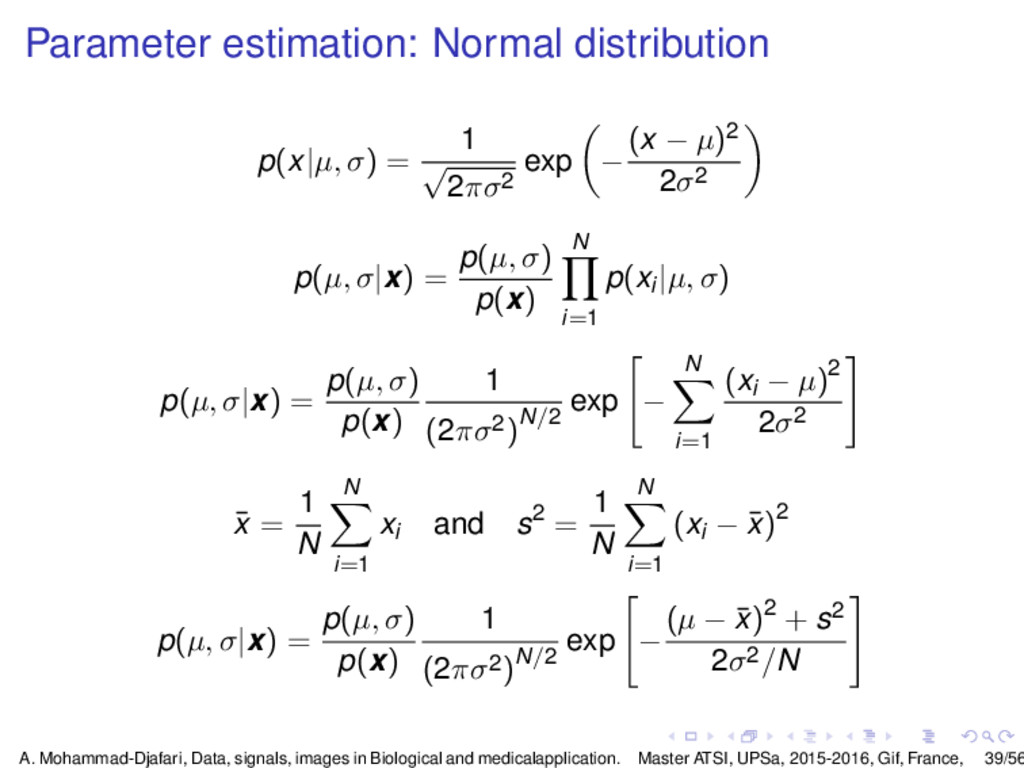
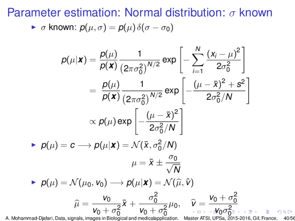
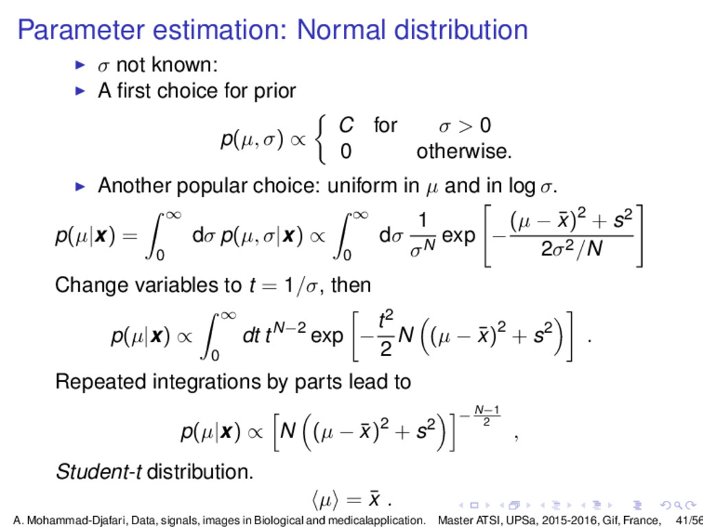
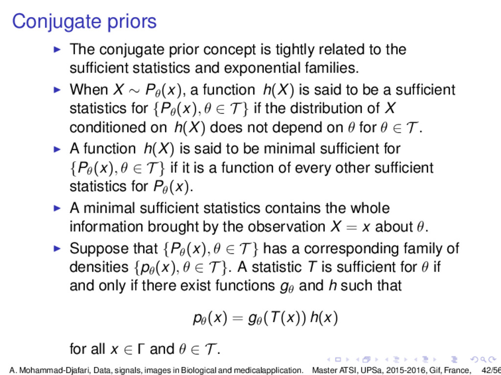
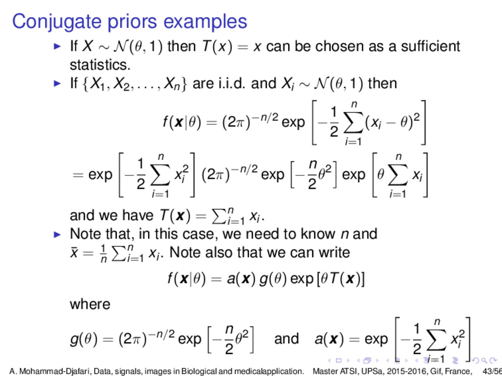
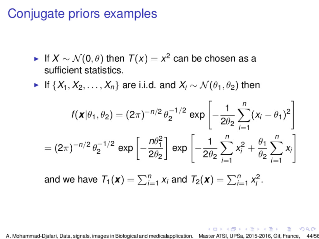
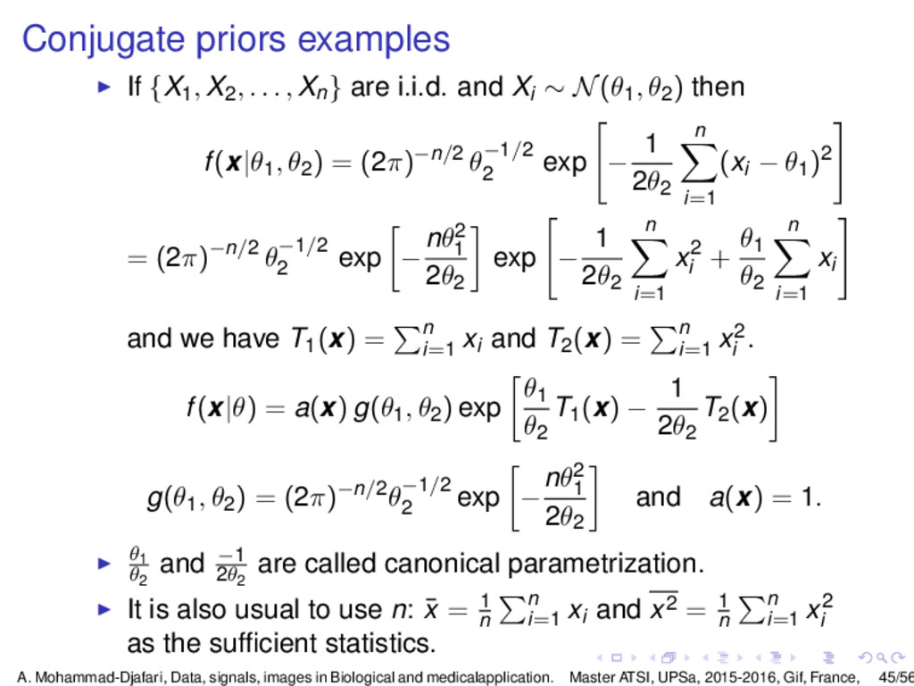
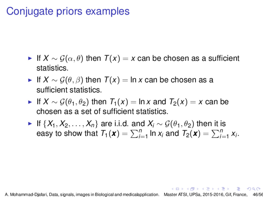
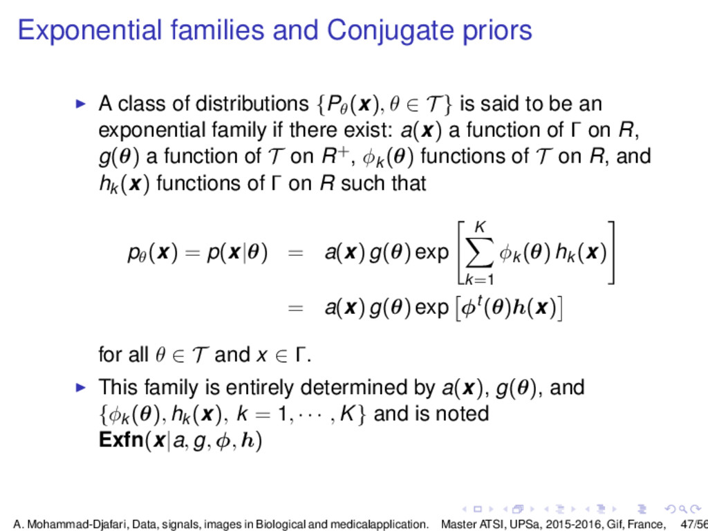
2. Summary 1: Data, signals, images in Biological and medical applications Individual cells, Population of cells, Small animals, Human In vitro and In Vivo A great number of data, variables, time series, signals, images, ... Genes expression, Hormones, temperature, ECG, EMG, ... Tomographic images (X rays, PET, SPECT, IRM), 3D body volume, fMRI, Holographic, multi- and Hyper-spectral images, ... Need for Visualization tools multicomponent, multivariate and multidimensional Time domain Transformed domain: Fourier, Wavelets, Time-Frequency... Scatter plots, histograms, statistics, ... A. Mohammad-Djafari, Data, signals, images in Biological and medicalapplication. Master ATSI, UPSa, 2015-2016, Gif, France, 2/56
3. Summary 1.1: Data, Signal, Image Data, Signal, Image Data: Unstructured Signal: Structured in time Image: Structured in space Extensions: 3D, Space-Time, Space-Frequency, .... Different representations Data: points in an abstract space, manifold Signal: time and frequency Image: space and spatial frequency Extensions: 3D, Space-Time, Space-Frequency, .... A. Mohammad-Djafari, Data, signals, images in Biological and medicalapplication. Master ATSI, UPSa, 2015-2016, Gif, France, 3/56
4. Summary 1.2: Data, unstructured One variable case Histogram and Probability distribution Parametric and Non parametric Parametric models: Method of moments Maximum Likehood Bayesian estimation Muti variable case Joint Histogram and Joint Probability distribution Correlation and Independence Conditional and Marginal pdfs Copula Related estimation problems A. Mohammad-Djafari, Data, signals, images in Biological and medicalapplication. Master ATSI, UPSa, 2015-2016, Gif, France, 4/56
5. Summary 2.1: Time series Time serie and Fourier representation Continuous / Discrete Correlation, Inter-correlation, Inter-dependance Stationarity / non-stationarity Convolution and Deconvolution Filtering and Denoising Modelling and Prediction Parametric and Non parametric models Parametric models: Least Squares Maximum Likehood Bayesian estimation A. Mohammad-Djafari, Data, signals, images in Biological and medicalapplication. Master ATSI, UPSa, 2015-2016, Gif, France, 5/56
6. Summary 2.2: Images Continuous / Discrete Gray and Color images 2D FT and FFT 2D Correlation and inter-correlation Stationarity / non-stationarity 2D Convolution Filtering and Denoising Modelling and Prediction Simple Markovian models Contours and Regions Hierarchical Markov models A. Mohammad-Djafari, Data, signals, images in Biological and medicalapplication. Master ATSI, UPSa, 2015-2016, Gif, France, 6/56
7. Summary 3: Data redundancy, Dimensionality Reduction, ... Redundancy and structure Dimentionality Reduction PCA and ICA PPCA and its extensions Stationarity / non-stationarity Discriminant Analysis (DA) Classification and Clustering Mixture Models Factor Analysis Blind Sources Separation A. Mohammad-Djafari, Data, signals, images in Biological and medicalapplication. Master ATSI, UPSa, 2015-2016, Gif, France, 7/56
8. Summary 4 to 8: Medical and Biological Applications Case studies Signals: Electro-Cardio-Gram (ECG) Electro-Encephalo-Gram (EEG) Electro-Myo-Gram (EMG) Magneto-Electro-Gram (MEG) Images: Computed Tomography: X ray CT Scan Magnetic Resonance Imaging (MRI) Positon Emission Tomography (PET) Single Photon Emission Computed Tomography (SPECT) Phosphorescence, Molecular Imaging Case studies in Cancer Research A. Mohammad-Djafari, Data, signals, images in Biological and medicalapplication. Master ATSI, UPSa, 2015-2016, Gif, France, 8/56
9. 1D data: one variable Data: xi, i = 1, · · · , M 1D plot, mean, median, variance No order: exchangeable histogram, probability distribution, Statistical modelling: expected value, variance, mode, median, Higher order moments, entropy Parametric, semi-parametric and Non Parametric modelling Parameter estimation: MM, ML, Bayesian Model selection: AIC, BIC, ... A. Mohammad-Djafari, Data, signals, images in Biological and medicalapplication. Master ATSI, UPSa, 2015-2016, Gif, France, 9/56
10. 1D data (Gaussian) 0 20 40 60 80 100 120 140 160 180 200 -3 -2 -1 0 1 2 3 Normal d ata001 -4 -3 -2 -1 0 1 2 3 0 5 10 15 20 25 30 −3 −2 −1 0 1 2 3 0 0.02 0.04 0.06 0.08 0.1 0.12 E=0.12323 V=0.9727 A. Mohammad-Djafari, Data, signals, images in Biological and medicalapplication. Master ATSI, UPSa, 2015-2016, Gif, France, 10/56
11. 1D data (Gamma) 0 20 40 60 80 100 120 140 160 180 200 0 1 2 3 4 5 6 7 Gamma d ata001 0 1 2 3 4 5 6 0 10 20 30 40 50 60 0 1 2 3 4 5 6 7 0 0.05 0.1 0.15 0.2 0.25 0.3 0.35 E=1.0291 V=1.0623 A. Mohammad-Djafari, Data, signals, images in Biological and medicalapplication. Master ATSI, UPSa, 2015-2016, Gif, France, 11/56
12. 1D data (Uniform) 0 20 40 60 80 100 120 140 160 180 200 0 0.1 0.2 0.3 0.4 0.5 0.6 0.7 0.8 0.9 1 Uniform d ata001 0 0.1 0.2 0.3 0.4 0.5 0.6 0.7 0.8 0.9 1 0 5 10 15 0 0.1 0.2 0.3 0.4 0.5 0.6 0.7 0.8 0.9 1 0 0.01 0.02 0.03 0.04 0.05 0.06 0.07 0.08 0.09 0.1 V=0.08125 A. Mohammad-Djafari, Data, signals, images in Biological and medicalapplication. Master ATSI, UPSa, 2015-2016, Gif, France, 12/56
13. 1D data: Statistics and probability modeling Statistics Mean, Variance, standard deviation, moments,... Histogram and probability distribution matching Uniform, Gaussian, Gamma,... shapes Probabilistic modelling Method of Moments (MM) Maximum Entropy (ME) Maximum Likelihood (ML) Bayesian estimation Non Parametric Bayesian methods A. Mohammad-Djafari, Data, signals, images in Biological and medicalapplication. Master ATSI, UPSa, 2015-2016, Gif, France, 13/56
14. Multi-component, multi-variate, multi-dimensional data bi-component: {(xi, yi)}, i = 1, · · · , M}, 2M elements bi-variate: {xi, i = 1, · · · , M}, {yj, j = 1, · · · , N}, M + N elements bi-dimensional: Images: xi,j, i = 1, · · · , M, j = 1, · · · , N, M ∗ N elements 0 20 40 60 80 100 120 140 160 180 200 -4 -3 -2 -1 0 1 2 3 2 data sets x i y j -2 0 2 -2 0 2 50 100 150 200 10 20 30 40 50 60 70 80 90 100 10 20 30 40 50 60 70 80 90 100 -3 -2 -1 0 1 2 3 A. Mohammad-Djafari, Data, signals, images in Biological and medicalapplication. Master ATSI, UPSa, 2015-2016, Gif, France, 14/56
15. Bi-component or Bi-variate data 2D distribution: joint probability distribution p(x, y) Conditionals p(x|y), p(y|x) Marginal distributions p(x), p(y) Expected values E(X), E(Y), variances V(X), V(Y), and Covariances, Higher order moments, entropy Independence tests Copula, ... 0 20 40 60 80 100 120 140 160 180 200 -4 -3 -2 -1 0 1 2 3 2 data sets x i y j 0 20 40 60 80 100 120 140 160 180 200 -4 -3 -2 -1 0 1 2 3 2 data sets x i y j x -3 -2 -1 0 1 2 3 4 y -3 -2 -1 0 1 2 3 1 A. Mohammad-Djafari, Data, signals, images in Biological and medicalapplication. Master ATSI, UPSa, 2015-2016, Gif, France, 15/56
16. Bivariate data Joint, marginals and conditional probability density functions x -2 0 2 y -3 -2 -1 0 1 2 20 15 10 5 20 15 10 5 0.14 0.12 0.1 0.08 0.06 0.04 0.02 0 3 2 1 x1 0 -1 -2 -2 -1 0 x2 1 2 0.14 0.12 0.1 0.08 0.06 0.04 0.02 Probability Density A. Mohammad-Djafari, Data, signals, images in Biological and medicalapplication. Master ATSI, UPSa, 2015-2016, Gif, France, 16/56
17. Probability theory Review: Discrete and Continuous variables probability laws What is a probability? What is a random variable? What are the main rules of probability Discrete probability laws: Bernouilli Binomial Poisson Continuous probability laws: Uniform U(.|a, b) Beta B(.|α, β) Gaussian N(.|µ, v) Generalized Gaussian GG(.|γ, β) Gamma G(.|α, β) Student-t S(.|ν, µ, λ) Cauchy C(.|µ, λ) A. Mohammad-Djafari, Data, signals, images in Biological and medicalapplication. Master ATSI, UPSa, 2015-2016, Gif, France, 17/56
18. Uniform and Beta distributions Uniform: X ∼ U(.|a, b) −→ p(x) = 1 b − a , x ∈ [a, b] E {X} = a + b 2 , Var {X} = (b − a)2 12 Beta: X ∼ Beta(.|α, β) −→ p(x) = 1 B(α, β) xα−1(1−x)β−1, x ∈ [0, 1] E {X} = α α + β , Var {X} = αβ (α + β)2(α + β + 1) Beta(.|1, 1) = U(.|0, 1) A. Mohammad-Djafari, Data, signals, images in Biological and medicalapplication. Master ATSI, UPSa, 2015-2016, Gif, France, 18/56
19. Uniform and Beta distributions A. Mohammad-Djafari, Data, signals, images in Biological and medicalapplication. Master ATSI, UPSa, 2015-2016, Gif, France, 19/56
20. Gaussian distributions Different notations: classical one with mean and variance: X ∼ N(.|µ, σ2) −→ p(x) = 1 √ 2πσ2 exp − 1 2σ2 (x − µ)2 E {X} = µ, Var {X} = σ2 mean and precision parameters: X ∼ N(.|µ, λ) −→ p(x) = λ √ 2π exp − λ 2 (x − µ)2 E {X} = µ, Var {X} = σ2 = 1 λ A. Mohammad-Djafari, Data, signals, images in Biological and medicalapplication. Master ATSI, UPSa, 2015-2016, Gif, France, 20/56
21. Generalized Gaussian distributions Gaussian: X ∼ N(.|µ, σ2) −→ p(x) = 1 √ 2πσ2 exp − 1 2 (x − µ) σ 2 Generalized Gaussian: X ∼ GG(.|α, β) −→ p(x) = β 2αΓ(1/β) exp − |x − µ| α β E {X} = µ, Var {X} = α2Γ(3/β) γ(1/β) β > 0, β = 1 Laplace, β = 2: Gaussian, β → ∞: Uniform A. Mohammad-Djafari, Data, signals, images in Biological and medicalapplication. Master ATSI, UPSa, 2015-2016, Gif, France, 21/56
22. Gaussian and Generalized Gaussian distributions A. Mohammad-Djafari, Data, signals, images in Biological and medicalapplication. Master ATSI, UPSa, 2015-2016, Gif, France, 22/56
23. Gamma distributions Forme 1: p(x|α, β) = βα Γ(α) xα−1e−βx for x ≥ 0 E {X} = α β , Var {X} = α β2 , Mod(X) = α − 1 α + β − 2 Forme 2: θ = 1/β p(x|α, θ) = θ−α Γ(α) xα−1e−x/β for x ≥ 0 α = 1: Exponential, 0 < α < 1 decreasing, α > 1 Mode=α−1 β A. Mohammad-Djafari, Data, signals, images in Biological and medicalapplication. Master ATSI, UPSa, 2015-2016, Gif, France, 23/56
24. Gamma distributions A. Mohammad-Djafari, Data, signals, images in Biological and medicalapplication. Master ATSI, UPSa, 2015-2016, Gif, France, 24/56
25. Student-t and Cauchy distributions Student’s t-distribution has the probability density function: p(x|ν) = Γ(ν+1 2 ) √ νπ Γ(ν 2 ) 1 + x2 ν −ν+1 2 = 1 √ ν B 1 2 , ν 2 1 + x2 ν −ν+1 2 where ν is the number of degrees of freedom, Γ is the Gamma function and B is the Beta function. ν = 1 gives Cauchy distribution. p(x) = π 1 + x2 Cauchy distribution: p(t|µ) = π 1 + (x − µ)2 A. Mohammad-Djafari, Data, signals, images in Biological and medicalapplication. Master ATSI, UPSa, 2015-2016, Gif, France, 25/56
26. Student-t and Cauchy distributions Three parameters location (µ) / scale (λ) / degree of freedom (ν) version p(x|µ, λ, ν) = Γ(ν+1 2 ) Γ(ν 2 ) λ πν 1 2 1 + λ(x − µ)2 ν −ν+1 2 E {X} = µ for ν > 1, Var {X} = 1 λ ν ν−2 for ν > 2, mode(X) = µ. Interesting relation between Student-t, Normal and Gamma distributions: S(x|µ, 1, ν) = N(x|µ, 1/λ) G(λ|ν/2, ν/2) dλ S(x|0, 1, ν) = N(x|0, 1/λ) G(λ|ν/2, ν/2) dλ A. Mohammad-Djafari, Data, signals, images in Biological and medicalapplication. Master ATSI, UPSa, 2015-2016, Gif, France, 26/56
27. Student and Cauchy p(x|ν) ∝ 1 + x2 ν −ν+1 2 A. Mohammad-Djafari, Data, signals, images in Biological and medicalapplication. Master ATSI, UPSa, 2015-2016, Gif, France, 27/56
28. Multivariate continuous probability laws Gaussian N(.|µ, V ) Student-t S(.|γ, β) Hyperbolic H(.|γ, β) A. Mohammad-Djafari, Data, signals, images in Biological and medicalapplication. Master ATSI, UPSa, 2015-2016, Gif, France, 28/56
29. Multivariate Gaussian Different notations: mean and covariance matrix (classical): X ∼ N(.|µ, σ) p(x) = (2π)−n/2|Σ|−1/2 exp − 1 2 (x − µ) Σ−1(x − µ) E {X} = µ, cov[X] = Σ mean and precision matrix: X ∼ N(.|µ, Λ) p(x) = (2π)−n/2|Λ|1/2 exp − 1 2 (x − µ) Λ(x − µ) E {X} = µ, cov[X] = Λ−1 A. Mohammad-Djafari, Data, signals, images in Biological and medicalapplication. Master ATSI, UPSa, 2015-2016, Gif, France, 29/56
30. Multivariate normal distributions A. Mohammad-Djafari, Data, signals, images in Biological and medicalapplication. Master ATSI, UPSa, 2015-2016, Gif, France, 30/56
31. Multivariate Student-t p(x|µ, Σ, ν) ∝ |Σ|−1/2 1 + 1 ν (x − µ) Σ−1(x − µ) (ν+p)/2 p = 1 f(t) = Γ((ν + 1)/2) Γ(ν/2) √ νπ (1 + t2/ν)−(ν+1) 2 p = 2, Σ−1 = A f(t1, t2) = Γ((ν + p)/2) Γ(ν/2) √ νpπp |A|1/2 2π  1 + p i=1 p j=1 Aij ti tj/ν   −(ν+2) 2 p = 2, Σ = A = I f(t1, t2) = 1 2π (1 + (t2 1 + t2 1 )/ν)−(ν+2) 2 A. Mohammad-Djafari, Data, signals, images in Biological and medicalapplication. Master ATSI, UPSa, 2015-2016, Gif, France, 31/56
32. Multivariate Student-t distributions A. Mohammad-Djafari, Data, signals, images in Biological and medicalapplication. Master ATSI, UPSa, 2015-2016, Gif, France, 32/56
33. Multivariate normal distributions Normal Student-t A. Mohammad-Djafari, Data, signals, images in Biological and medicalapplication. Master ATSI, UPSa, 2015-2016, Gif, France, 33/56
34. Multivariate elliptic p(x|µ, Σ, ν) ∝ g 1 + 1 ν (x − µ) Σ−1(x − µ) g(z) = exp [−z/2] −→ Multivariate normal More general: Caracteristic function exp ix µ Ψ(x Σx) A. Mohammad-Djafari, Data, signals, images in Biological and medicalapplication. Master ATSI, UPSa, 2015-2016, Gif, France, 34/56
35. Multivariate Wishart Suppose X is an n × p matrix, each row of which is independently drawn from a p-variate normal distribution with zero mean: Xi = [x1 i , . . . , xp i ] ∼ Np(.|0, V ) Then the Wishart distribution is the probability distribution of the p × p random matrix S = X X known as the scatter matrix: S ∼ Wp(.|V , ν). The positive integer ν is the number of degrees of freedom. Sometimes this is written W(V , p, ν). For n ≥ p the matrix S is invertible with probability 1 if V is invertible. If p = 1 and V = 1 then this distribution is a chi-squared distribution with ν degrees of freedom A. Mohammad-Djafari, Data, signals, images in Biological and medicalapplication. Master ATSI, UPSa, 2015-2016, Gif, France, 35/56
36. Multivariate Wishart probability density: p(S|V , ν) = |S|(ν−p−1)/2 exp −1 2 Tr(V −1S) 2νp/2 |V |ν/2 Γp(ν/2) where Γp(.) is the multivariate gamma function defined as Γp(ν/2) = πp(p−1)/4Πp j=1 Γ [ν/2 + (1 − j)/2] . E {S} = V , Var Sij = ν(v2 ij + vii vjj) A. Mohammad-Djafari, Data, signals, images in Biological and medicalapplication. Master ATSI, UPSa, 2015-2016, Gif, France, 36/56
37. Parameter estimation We observe n samples x = {x1, · · · , xn} of a quantity X whose pdf depends on certain parameters θ: p(x|θ). The question is to determine θ. Moments method: E xk = xk p(x|θ) dx ≈ 1 n n i=1 xk i , k = 1, · · · , K Maximum Likelihood L(θ) = n i=1 p(xi|θ) or ln L(θ) = n i=1 ln p(xi|θ) θ = arg max θ {L(θ)} = arg min θ {− ln L(θ)} Bayesian approach A. Mohammad-Djafari, Data, signals, images in Biological and medicalapplication. Master ATSI, UPSa, 2015-2016, Gif, France, 37/56
38. Bayesian Parameter estimation Likelihood p(x|θ) = n i=1 p(xi|θ) A priori p(θ) A posteriori p(θ|x) ∝ p(x|θ)p(θ) Infer on θ using p(θ|x). For example: Maximum A Posteriori (MAP) θ = arg max θ {p(θ|x)} Posterior Mean θ = θp(θ|x) dθ A. Mohammad-Djafari, Data, signals, images in Biological and medicalapplication. Master ATSI, UPSa, 2015-2016, Gif, France, 38/56
39. Parameter estimation: Normal distribution p(x|µ, σ) = 1 √ 2πσ2 exp − (x − µ)2 2σ2 p(µ, σ|x) = p(µ, σ) p(x) N i=1 p(xi|µ, σ) p(µ, σ|x) = p(µ, σ) p(x) 1 (2πσ2)N/2 exp − N i=1 (xi − µ)2 2σ2 ¯ x = 1 N N i=1 xi and s2 = 1 N N i=1 (xi − ¯ x)2 p(µ, σ|x) = p(µ, σ) p(x) 1 (2πσ2)N/2 exp − (µ − ¯ x)2 + s2 2σ2/N A. Mohammad-Djafari, Data, signals, images in Biological and medicalapplication. Master ATSI, UPSa, 2015-2016, Gif, France, 39/56
40. Parameter estimation: Normal distribution: σ known σ known: p(µ, σ) = p(µ) δ(σ − σ0) p(µ|x) = p(µ) p(x) 1 2πσ2 0 N/2 exp − N i=1 (xi − µ)2 2σ2 0 = p(µ) p(x) 1 2πσ2 0 N/2 exp − (µ − ¯ x)2 + s2 2σ2 0 /N ∝ p(µ) exp − (µ − ¯ x)2 2σ2 0 /N p(µ) = c −→ p(µ|x) = N(¯ x, σ2 0 /N) µ = ¯ x ± σ0 √ N p(µ) = N(µ0, v0) −→ p(µ|x) = N(µ, ˆ v) µ = v0 v0 + σ2 0 ¯ x + σ2 0 v0 + σ2 0 µ0, v = v0 + σ2 0 v0σ2 0 A. Mohammad-Djafari, Data, signals, images in Biological and medicalapplication. Master ATSI, UPSa, 2015-2016, Gif, France, 40/56
41. Parameter estimation: Normal distribution σ not known: A first choice for prior p(µ, σ) ∝ C for σ > 0 0 otherwise. Another popular choice: uniform in µ and in log σ. p(µ|x) = ∞ 0 dσ p(µ, σ|x) ∝ ∞ 0 dσ 1 σN exp − (µ − ¯ x)2 + s2 2σ2/N Change variables to t = 1/σ, then p(µ|x) ∝ ∞ 0 dt tN−2 exp − t2 2 N (µ − ¯ x)2 + s2 . Repeated integrations by parts lead to p(µ|x) ∝ N (µ − ¯ x)2 + s2 −N−1 2 , Student-t distribution. µ = ¯ x . A. Mohammad-Djafari, Data, signals, images in Biological and medicalapplication. Master ATSI, UPSa, 2015-2016, Gif, France, 41/56
42. Conjugate priors The conjugate prior concept is tightly related to the sufficient statistics and exponential families. When X ∼ Pθ(x), a function h(X) is said to be a sufficient statistics for {Pθ(x), θ ∈ T } if the distribution of X conditioned on h(X) does not depend on θ for θ ∈ T . A function h(X) is said to be minimal sufficient for {Pθ(x), θ ∈ T } if it is a function of every other sufficient statistics for Pθ(x). A minimal sufficient statistics contains the whole information brought by the observation X = x about θ. Suppose that {Pθ(x), θ ∈ T } has a corresponding family of densities {pθ(x), θ ∈ T }. A statistic T is sufficient for θ if and only if there exist functions gθ and h such that pθ(x) = gθ(T(x)) h(x) for all x ∈ Γ and θ ∈ T . A. Mohammad-Djafari, Data, signals, images in Biological and medicalapplication. Master ATSI, UPSa, 2015-2016, Gif, France, 42/56
43. Conjugate priors examples If X ∼ N(θ, 1) then T(x) = x can be chosen as a sufficient statistics. If {X1, X2, . . . , Xn} are i.i.d. and Xi ∼ N(θ, 1) then f(x|θ) = (2π)−n/2 exp − 1 2 n i=1 (xi − θ)2 = exp − 1 2 n i=1 x2 i (2π)−n/2 exp − n 2 θ2 exp θ n i=1 xi and we have T(x) = n i=1 xi . Note that, in this case, we need to know n and ¯ x = 1 n n i=1 xi . Note also that we can write f(x|θ) = a(x) g(θ) exp [θT(x)] where g(θ) = (2π)−n/2 exp − n 2 θ2 and a(x) = exp − 1 2 n i=1 x2 i A. Mohammad-Djafari, Data, signals, images in Biological and medicalapplication. Master ATSI, UPSa, 2015-2016, Gif, France, 43/56
44. Conjugate priors examples If X ∼ N(0, θ) then T(x) = x2 can be chosen as a sufficient statistics. If {X1, X2, . . . , Xn} are i.i.d. and Xi ∼ N(θ1, θ2) then f(x|θ1, θ2) = (2π)−n/2 θ−1/2 2 exp − 1 2θ2 n i=1 (xi − θ1)2 = (2π)−n/2 θ−1/2 2 exp − nθ2 1 2θ2 exp − 1 2θ2 n i=1 x2 i + θ1 θ2 n i=1 xi and we have T1(x) = n i=1 xi and T2(x) = n i=1 x2 i . A. Mohammad-Djafari, Data, signals, images in Biological and medicalapplication. Master ATSI, UPSa, 2015-2016, Gif, France, 44/56
45. Conjugate priors examples If {X1, X2, . . . , Xn} are i.i.d. and Xi ∼ N(θ1, θ2) then f(x|θ1, θ2) = (2π)−n/2 θ−1/2 2 exp − 1 2θ2 n i=1 (xi − θ1)2 = (2π)−n/2 θ−1/2 2 exp − nθ2 1 2θ2 exp − 1 2θ2 n i=1 x2 i + θ1 θ2 n i=1 xi and we have T1(x) = n i=1 xi and T2(x) = n i=1 x2 i . f(x|θ) = a(x) g(θ1, θ2) exp θ1 θ2 T1(x) − 1 2θ2 T2(x) g(θ1, θ2) = (2π)−n/2θ−1/2 2 exp − nθ2 1 2θ2 and a(x) = 1. θ1 θ2 and −1 2θ2 are called canonical parametrization. It is also usual to use n: ¯ x = 1 n n i=1 xi and x2 = 1 n n i=1 x2 i as the sufficient statistics. A. Mohammad-Djafari, Data, signals, images in Biological and medicalapplication. Master ATSI, UPSa, 2015-2016, Gif, France, 45/56
46. Conjugate priors examples If X ∼ G(α, θ) then T(x) = x can be chosen as a sufficient statistics. If X ∼ G(θ, β) then T(x) = ln x can be chosen as a sufficient statistics. If X ∼ G(θ1, θ2) then T1(x) = ln x and T2(x) = x can be chosen as a set of sufficient statistics. If {X1, X2, . . . , Xn} are i.i.d. and Xi ∼ G(θ1, θ2) then it is easy to show that T1(x) = n i=1 ln xi and T2(x) = n i=1 xi . A. Mohammad-Djafari, Data, signals, images in Biological and medicalapplication. Master ATSI, UPSa, 2015-2016, Gif, France, 46/56
47. Exponential families and Conjugate priors A class of distributions {Pθ(x), θ ∈ T } is said to be an exponential family if there exist: a(x) a function of Γ on R, g(θ) a function of T on R+, φk (θ) functions of T on R, and hk (x) functions of Γ on R such that pθ(x) = p(x|θ) = a(x) g(θ) exp K k=1 φk (θ) hk (x) = a(x) g(θ) exp φt (θ)h(x) for all θ ∈ T and x ∈ Γ. This family is entirely determined by a(x), g(θ), and {φk (θ), hk (x), k = 1, · · · , K} and is noted Exfn(x|a, g, φ, h) A. Mohammad-Djafari, Data, signals, images in Biological and medicalapplication. Master ATSI, UPSa, 2015-2016, Gif, France, 47/56
48. Exponential families and Conjugate priors When a(x) = 1 and g(θ) = exp [−b(θ)] we have p(x|θ) = exp φt (θ)h(x) − b(θ) Natural exponential family: When a(x) = 1, g(θ) = exp [−b(θ)], h(x) = x and φ(θ) = θ we have p(x|θ) = exp θt x − b(θ) Scalar random variable with a vector parameter: p(x|θ) = a(x)g(θ) exp K k=1 φk (θ)hk (x) = a(x)g(θ) exp φt (θ)h(x) Scalar random variable with a scalar parameter: p(x|θ) = Exf(x|a, g, φ, h) = a(x)g(θ) exp [φ(θ)h(x)] p(x|θ) = θ exp [−θx] = exp [−θx + ln θ] , x ≥ 0, θ ≥ 0. A. Mohammad-Djafari, Data, signals, images in Biological and medicalapplication. Master ATSI, UPSa, 2015-2016, Gif, France, 48/56
49. Exponential families and Conjugate priors A family F of probability distributions π(θ) on T is said to be conjugate (or closed under sampling) if, for every π(θ) ∈ F, the posterior distribution π(θ|x) also belongs to F. Assume that f(x|θ) = l(θ|x) = l(θ|t(x)) where t = {n, s} = {n, s1, . . . , sk } is a vector of dimension k + 1 and is sufficient statistics for f(x|θ). Then, if there exists a vector {τ0, τ} = {τ0, τ1, . . . , τk } such that π(θ|τ) = f(s = (τ1, · · · , τk )|θ, n = τ0) f(s = (τ1, · · · , τk )|θ , n = τ0) dθ exists and defines a family F of distributions for θ ∈ T , then the posterior π(θ|x, τ) will remain in the same family F. The prior distribution π(θ|τ) is then a conjugate prior for the sampling distribution f(x|θ). A. Mohammad-Djafari, Data, signals, images in Biological and medicalapplication. Master ATSI, UPSa, 2015-2016, Gif, France, 49/56
50. Exponential families and Conjugate priors For a set of n i.i.d. samples {x1, · · · , xn} of a random variable X ∼ Exf(x|a, g, θ, h) we have f(x|θ) = n j=1 f(xj|θ) = [g(θ)]n   n j=1 a(xj)   exp   K k=1 φk (θ) n j=1 hk (xj)   = gn(θ) a(x) exp  φt (θ) n j=1 h(xj)   , where a(x) = n j=1 a(xj). Then, using the factorization theorem it is easy to see that t =    n, n j=1 h1(xj), · · · , n j=1 hK (xj)    is a sufficient statistics for θ. A. Mohammad-Djafari, Data, signals, images in Biological and medicalapplication. Master ATSI, UPSa, 2015-2016, Gif, France, 50/56
51. Exponential families and Conjugate priors A conjugate prior family for the exponential family f(x|θ) = a(x) g(θ) exp K k=1 φk (θ) hk (x) is given by π(θ|τ0, τ) = z(τ)[g(θ)]τ0 exp K k=1 τk φk (θ) The associated posterior law is π(θ|x, τ0, τ) ∝ [g(θ)]n+τ0 a(x)z(τ) exp   K k=1  τk + n j=1 hk (xj)   φk A. Mohammad-Djafari, Data, signals, images in Biological and medicalapplication. Master ATSI, UPSa, 2015-2016, Gif, France, 51/56
52. Exponential families and Conjugate priors If f(x|θ) = Exfn(x|a(x), g(θ), φ, h), then a conjugate prior family is π(θ|τ) = Exfn(θ|gτ0 , z(τ), τ, φ), and the associated posterior law is π(θ|x, τ) = Exfn(θ|gn+τ0 , a(x) z(τ), τ , φ) where τk = τk + n j=1 hk (xj) or τ = τ + ¯ h, with ¯ hk = n j=1 hk (xj). A. Mohammad-Djafari, Data, signals, images in Biological and medicalapplication. Master ATSI, UPSa, 2015-2016, Gif, France, 52/56
53. Exponential families and Conjugate priors If f(x|θ) = a(x) exp θt x − b(θ) Then a conjugate prior family is π(θ|τ0) = g(θ) exp τt 0 θ − d(τ0) and the corresponding posterior is π(θ|x, τ0) = g(θ) exp τt n θ − d(τn) with τn = τ0 + ¯ x where ¯ xn = 1 n n j=1 xj A. Mohammad-Djafari, Data, signals, images in Biological and medicalapplication. Master ATSI, UPSa, 2015-2016, Gif, France, 53/56
54. Exponential families and Conjugate priors f(x|θ) = a(x) exp θt x − b(θ) π(θ|α0, τ0) = g(α0, τ0) exp α0 τt 0 θ − α0b(τ0) π(θ|α0, τ0, x) = g(α, τ) exp α τt θ − αb(τ) α = α0 + n and τ = α0τ0 + n¯ x (α0 + n) ) E {X|θ} = E ¯ X|θ = ∇b(θ) E {∇b(Θ)|α0, τ0} = τ0 E {∇b(θ)|α0, τ0, x} = n¯ x + α0τ0 α0 + n = π¯ xn + (1 − π)τ0, with π = n α0+n A. Mohammad-Djafari, Data, signals, images in Biological and medicalapplication. Master ATSI, UPSa, 2015-2016, Gif, France, 54/56
55. Conjugate priors Observation law p(x|θ) Prior law p(θ|τ) Posterior law p(θ|x, τ) ∝ p(θ|τ)p(x|θ) Binomial Bin(x|n, θ) Beta Bet(θ|α, β) Beta Bet(θ|α + x, β + n − x) Negative Binomial NegBin(x|n, θ) Beta Bet(θ|α, β) Beta Bet(θ|α + n, β + x) Multinomial Mk (x|θ1, · · · , θk ) Dirichlet Dik (θ|α1, · · · , αk ) Dirichlet Dik (θ|α1 + x1, · · · , αk + xk ) Poisson Pn(x|θ) Gamma Gam(θ|α, β) Gamma Gam(θ|α + x, β + 1) A. Mohammad-Djafari, Data, signals, images in Biological and medicalapplication. Master ATSI, UPSa, 2015-2016, Gif, France, 55/56
56. Conjugate priors Observation law p(x|θ) Prior law p(θ|τ) Posterior law p(θ|x, τ) ∝ p(θ|τ)p(x Gamma Gam(x|ν, θ) Gamma Gam(θ|α, β) Gamma Gam(θ|α + ν, β + x) Beta Bet(x|α, θ) Exponential Ex(θ|λ) Exponential Ex(θ|λ − log(1 − x)) Normal N(x|θ, σ2) Normal N(θ|µ, τ2) Normal N µ|µσ2+τ2x σ2+τ2 , σ2 τ2 σ2+τ2 Normal N(x|µ, 1/θ) Gamma Gam(θ|α, β) Gamma Gam θ|α + 1 2 , β + 1 2 Normal N(x|θ, θ2) Generalized inverse Normal INg(θ|α, µ, σ) ∝ |θ|−α exp − 1 2σ2 1 θ − µ 2 Generalized inverse INg(θ|αn, µn, σn) A. Mohammad-Djafari, Data, signals, images in Biological and medicalapplication. Master ATSI, UPSa, 2015-2016, Gif, France, 56/56