Soft Introduction to MSE based Linear Regression

Talk from Lunch&Learn event at Azimo company 16/11/2017.

Transcript

1. Let’s solve a simple problem with Machine Learning!
2. House prices in Cracow
3. Randomly picked 38 house prices 22 164 22 380 35 175 35 320 36 199 36 198 37 320 38 210 38 199 39 295 41 315 41 299 45 315 48 359 49 285 50 279 50 409 50 286 51 330 52 380 54 375 54 396 54 430 54 299 56 387 56 465 59 285 60 295 62 485 62 314 67 500 69 390 74 459 75 498 75 460 78 550 Area [m^2] Area [m^2] Price [k zł] Price [k zł]
4. Visualise it
5. Problem
6. I have 83 meters square flat to sell.
7. I have 83 meters square flat to sell. What price should I set to match the market and don’t lose money? ?
8. We want our machine to be intelligent enough to solve it. But first engineer has to create that “intelligence” by implementing learning algorithm in code. But engineer has to know what code to write. He/she needs some instruction. Luckily math can be turned into code easily!
9. Linear Regression To solve the problem we will use Algorithm that will try to approximate all points with single line
10. Simple problem 0 0 1 1 2 2 3 3 x y
11. Simple problem 0 0 1 1 2 2 3 3 x y We want machine to find equation of linear function h(x) that will be as close as possible to fit all the points - ideally goes through all of them.
12. Simple problem 0 0 1 1 2 2 3 3 x y Linear function: y = a*x + b Machine will need to find right values for parameters a and b so the line goes ideally through all the points.
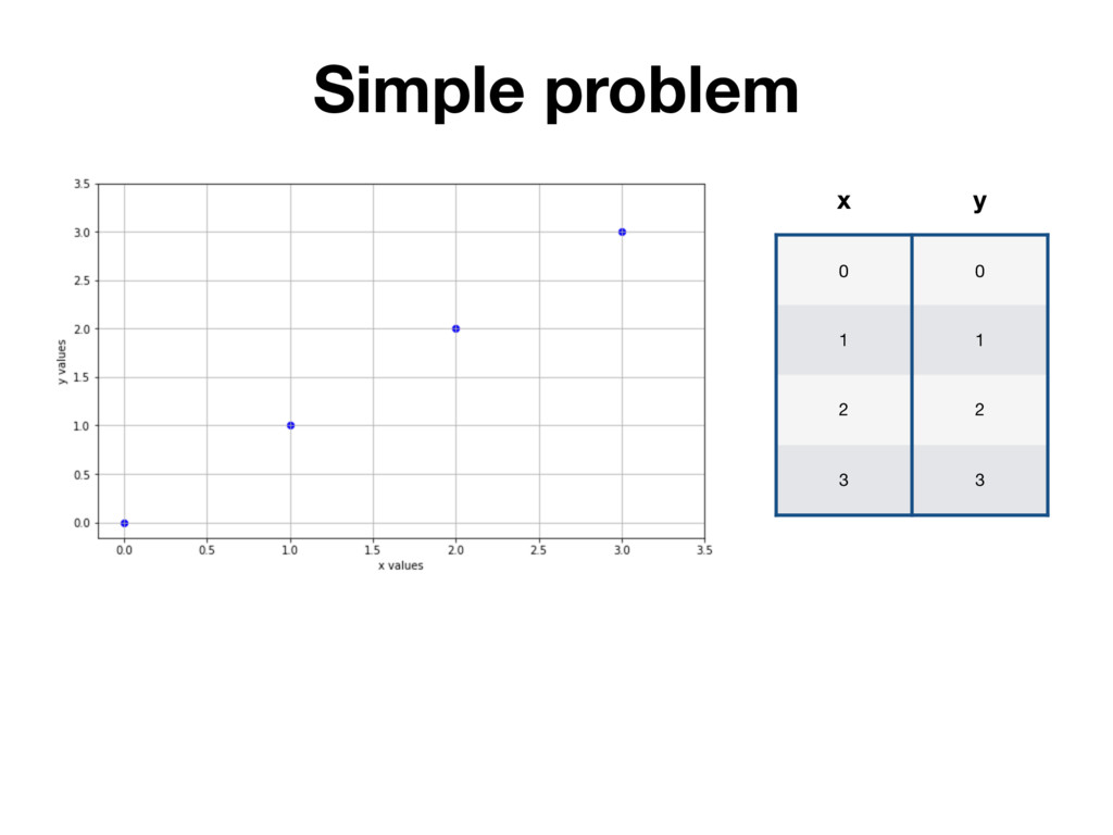
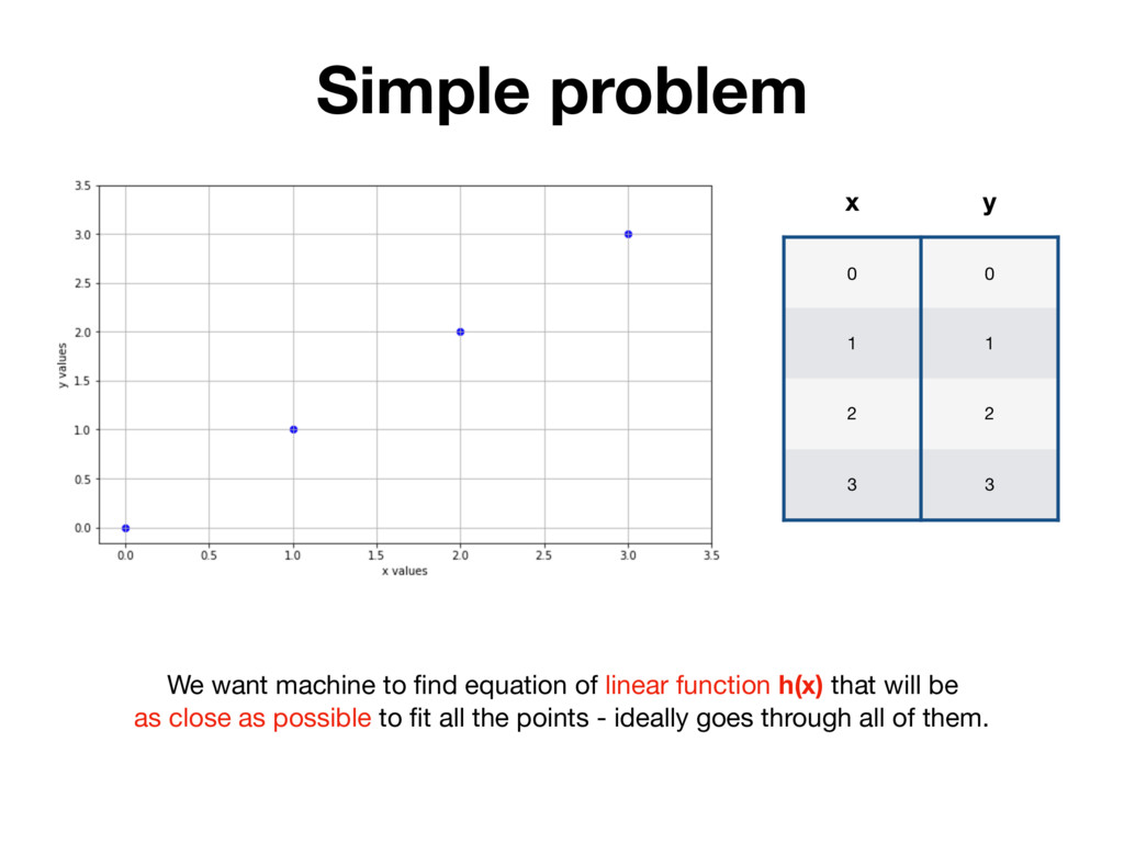
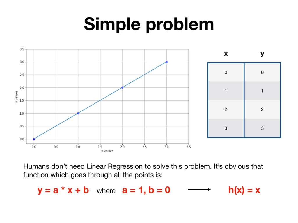
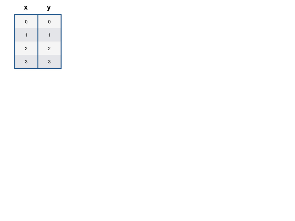
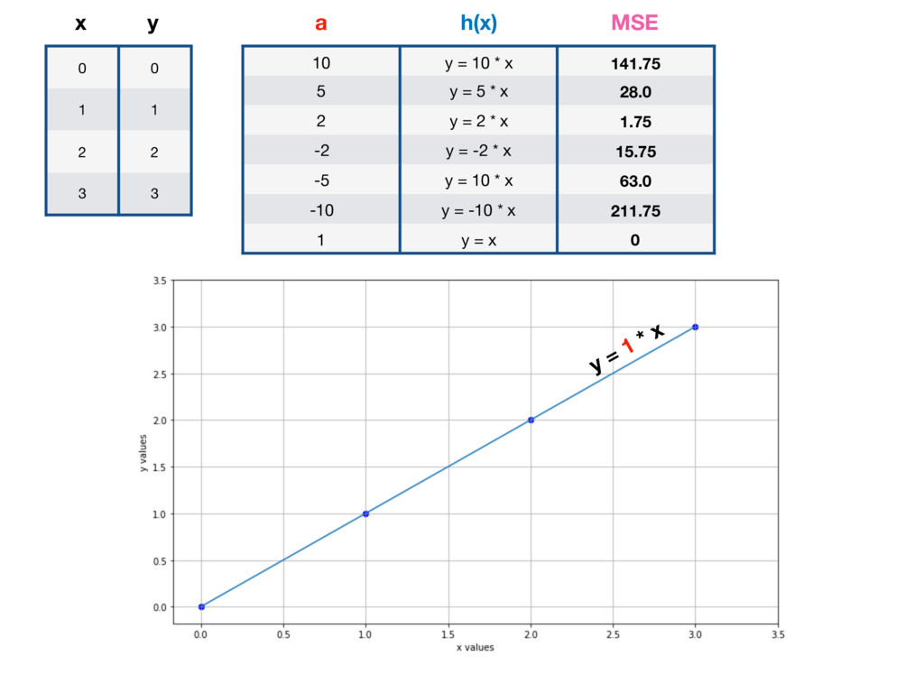
13. Simple problem 0 0 1 1 2 2 3 3 x y Humans don’t need Linear Regression to solve this problem. It’s obvious that function which goes through all the points is: h(x) = x y = a * x + b where a = 1, b = 0
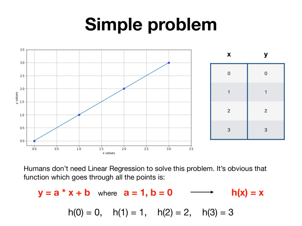
14. Simple problem 0 0 1 1 2 2 3 3 x y Humans don’t need Linear Regression to solve this problem. It’s obvious that function which goes through all the points is: h(x) = x y = a * x + b where a = 1, b = 0 h(0) = 0, h(1) = 1, h(2) = 2, h(3) = 3
15. But can you find a and b so for function h(x) fits those points as close as possible?
16. How to compare parameters? 0 0 1 1 2 2 3 3 x y Which parameters will create h(x) closest to all points? a = 0.5, b = 0 h(x) = 0.5x a = 0, b = 1.5 h(x) = 1.5
17. Let’s draw red and green functions 0 0 0 1.5 1 1 0.5 1.5 2 2 1 1.5 3 3 1.5 1.5 x h(x) = 0.5x h(x) = 1.5 y
18. Let’s draw red and green functions 0 0 0 1.5 1 1 0.5 1.5 2 2 1 1.5 3 3 1.5 1.5 x h(x) = 0.5x h(x) = 1.5 y
19. Let’s draw red and green functions 0 0 0 1.5 1 1 0.5 1.5 2 2 1 1.5 3 3 1.5 1.5 x h(x) = 0.5x h(x) = 1.5 y
20. Let’s calculate distance on y axis between corresponding points. r0 r1 r2 r3 g0 g1 g2 g3 Distance Red = r0 + r1 + r2 + r3 Distance Green = g0 + g1 + g2 + g3
21. r0 r1 r2 r3 Distance Red 0 0 0 1 1 0.5 2 2 1 3 3 1.5 x h(x) = 0.5x y r0 = 0 - 0 = 0
22. r0 r1 r2 r3 Distance Red 0 0 0 1 1 0.5 2 2 1 3 3 1.5 x h(x) = 0.5x y r0 = 0 - 0 = 0 r1 = 0.5 - 1 = -0.5
23. r0 r1 r2 r3 Distance Red 0 0 0 1 1 0.5 2 2 1 3 3 1.5 x h(x) = 0.5x y r0 = 0 - 0 = 0 r1 = 0.5 - 1 = -0.5 r2 = 1 - 2 = -1
24. r0 r1 r2 r3 Distance Red 0 0 0 1 1 0.5 2 2 1 3 3 1.5 x h(x) = 0.5x y r0 = 0 - 0 = 0 r1 = 0.5 - 1 = -0.5 r2 = 1 - 2 = -1 r3 = 1.5 - 3 = -1.5
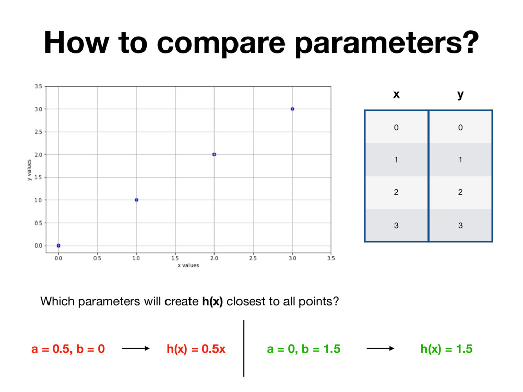
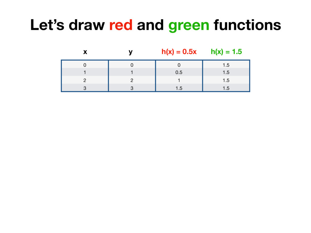
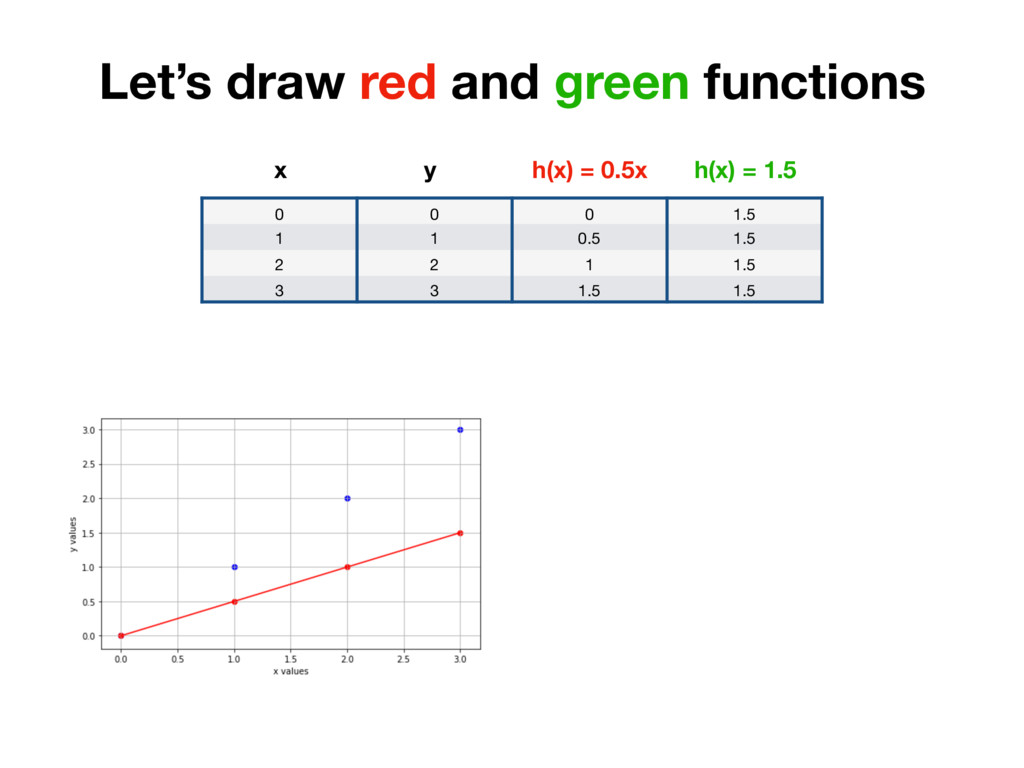
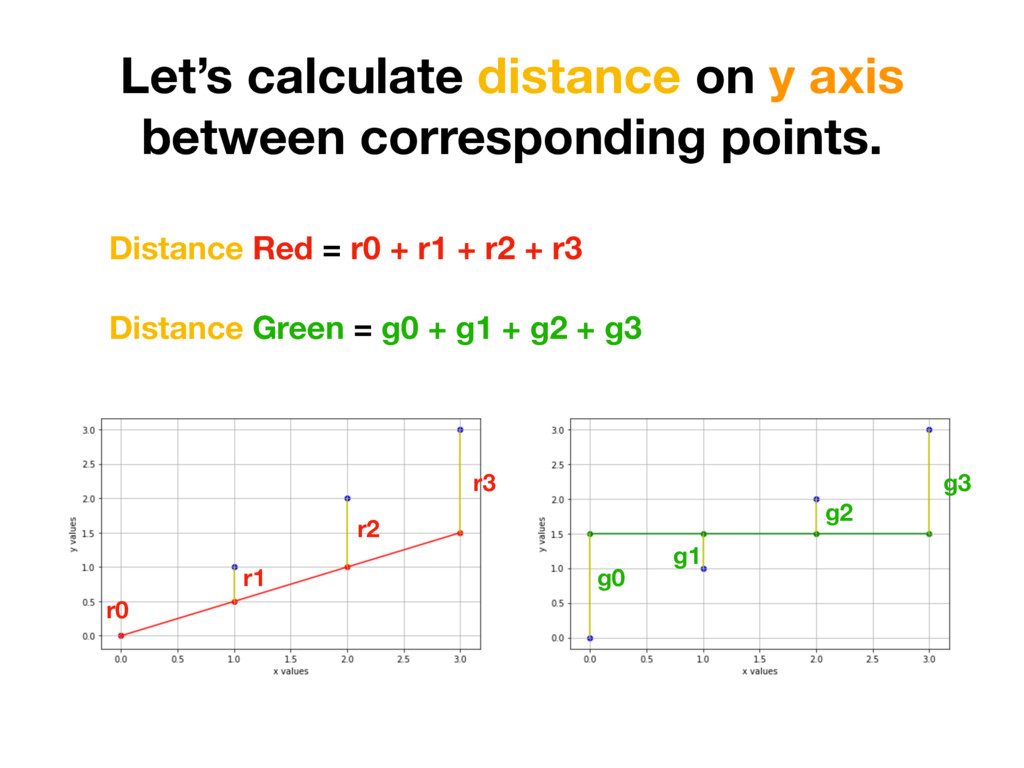
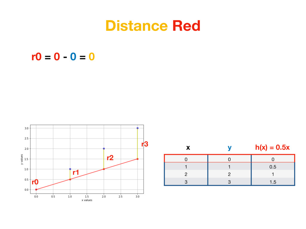
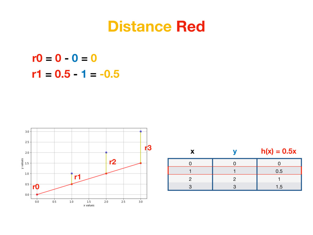
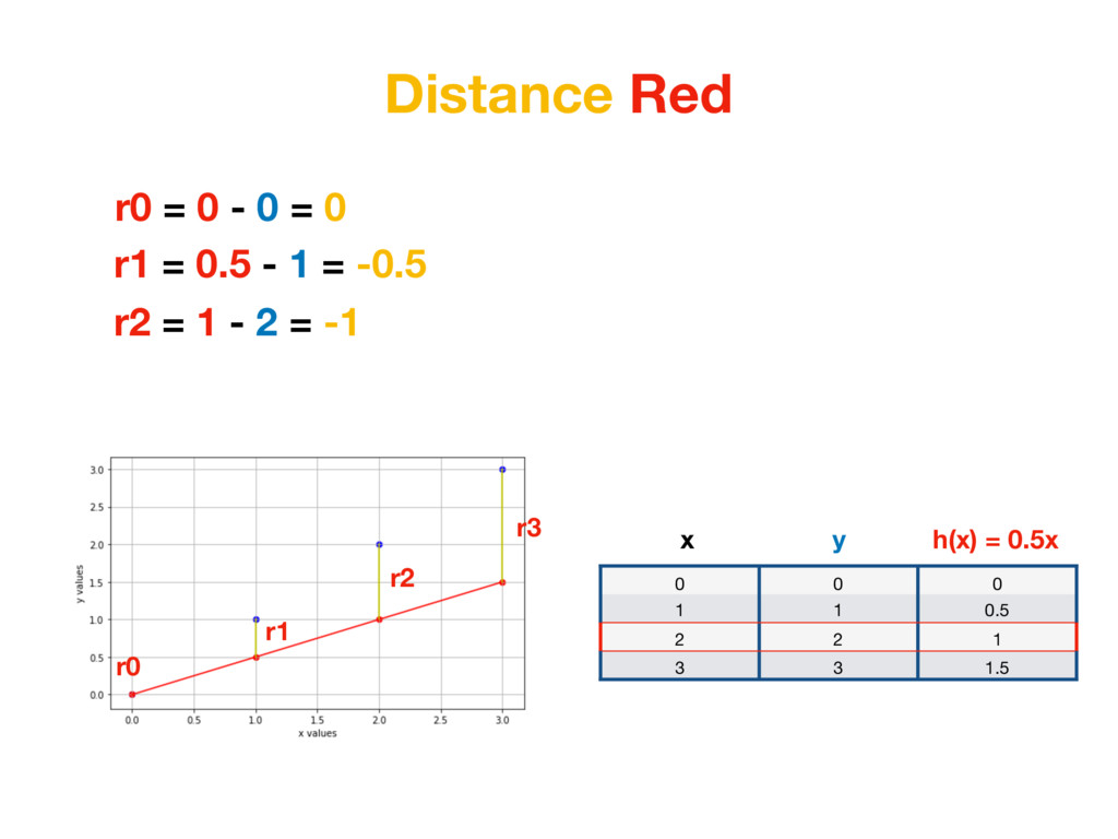
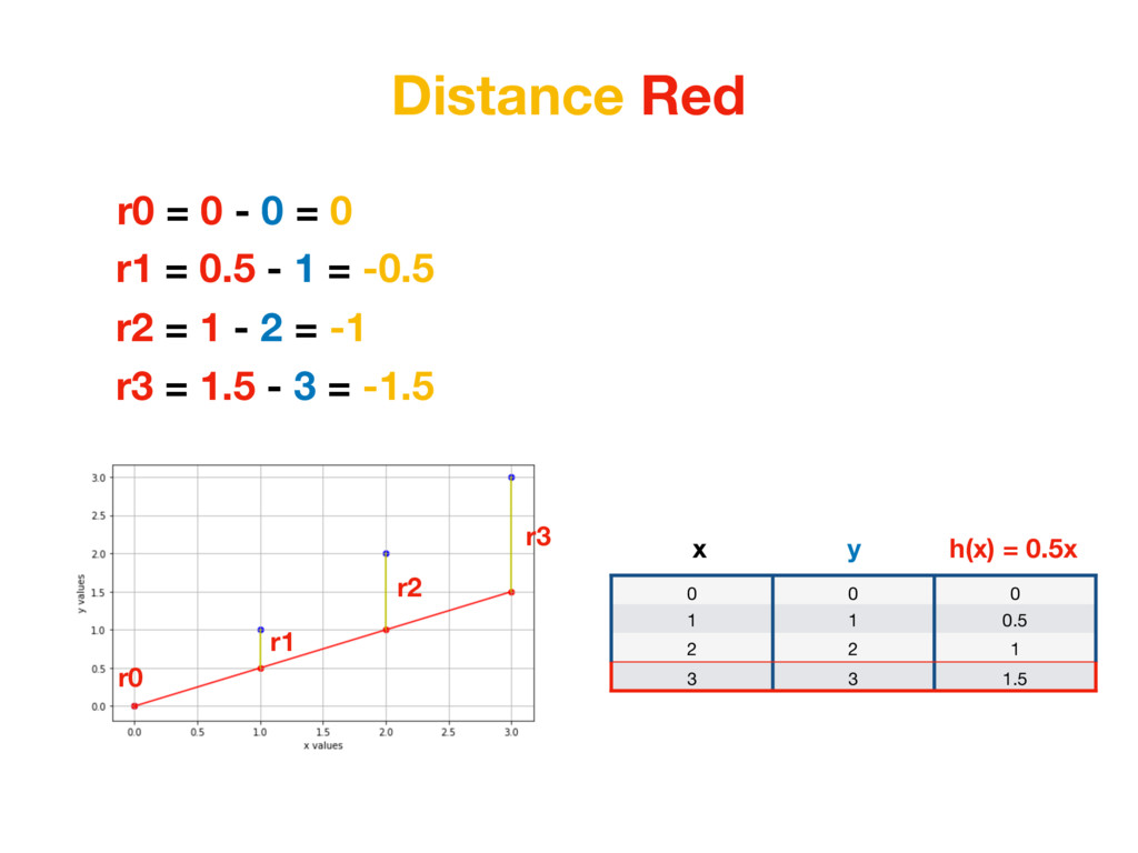
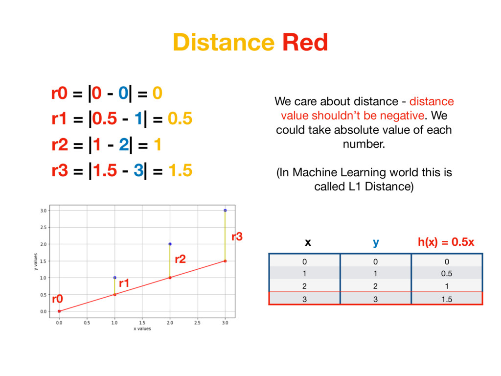
25. r0 r1 r2 r3 Distance Red 0 0 0 1 1 0.5 2 2 1 3 3 1.5 x h(x) = 0.5x y r0 = |0 - 0| = 0 r1 = |0.5 - 1| = 0.5 r2 = |1 - 2| = 1 r3 = |1.5 - 3| = 1.5 We care about distance - distance value shouldn’t be negative. We could take absolute value of each number. (In Machine Learning world this is called L1 Distance)
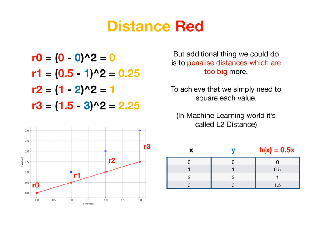
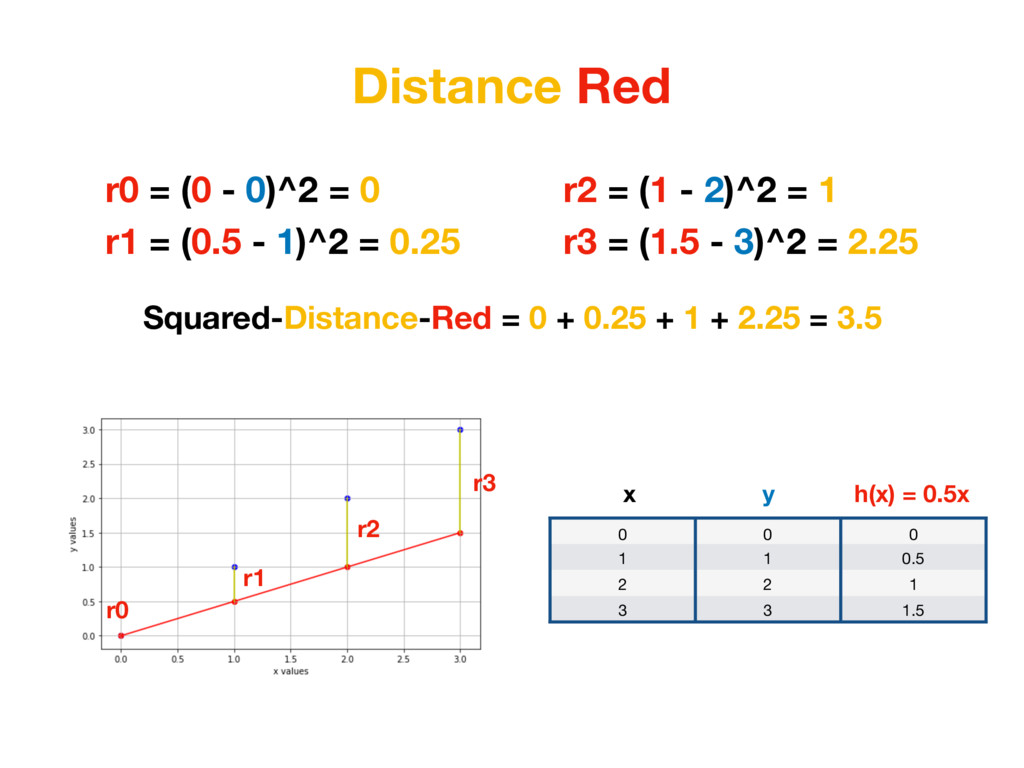
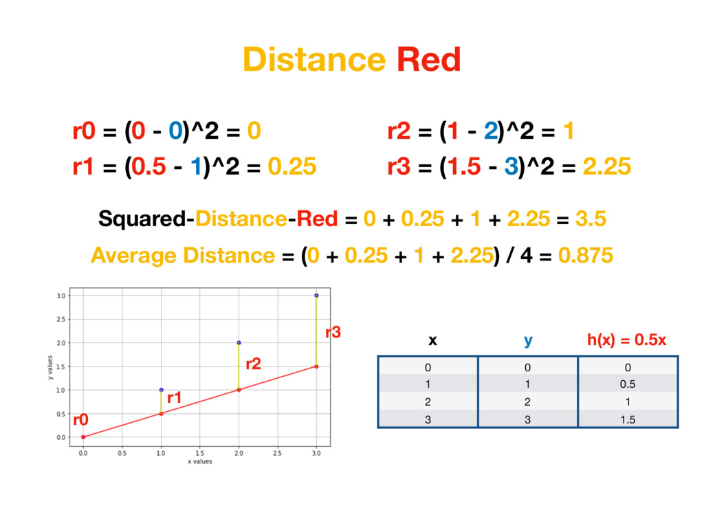
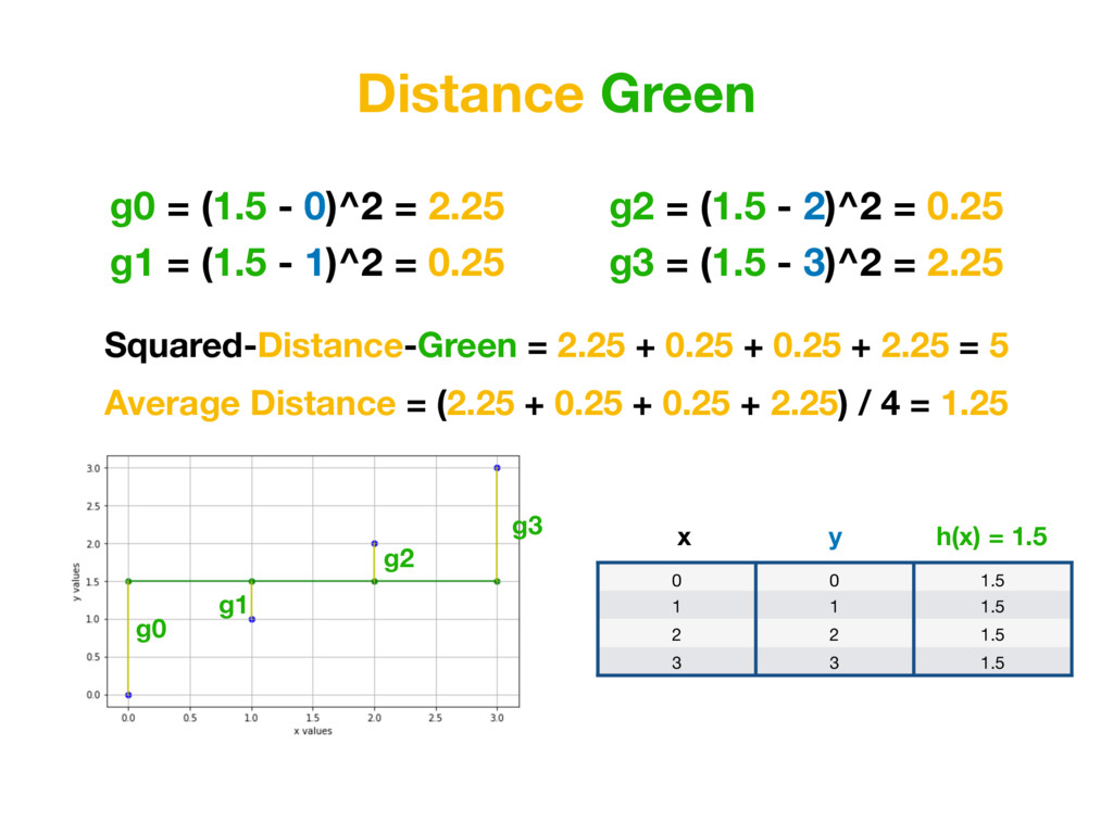
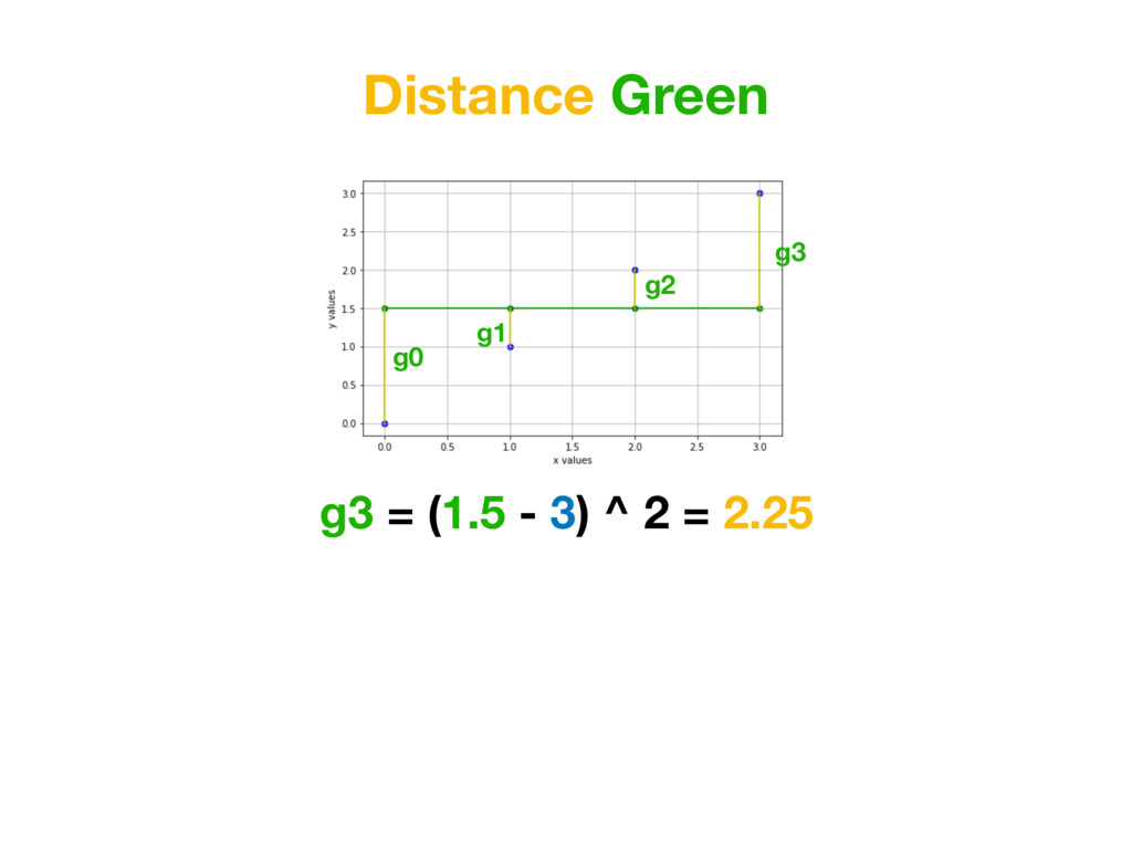
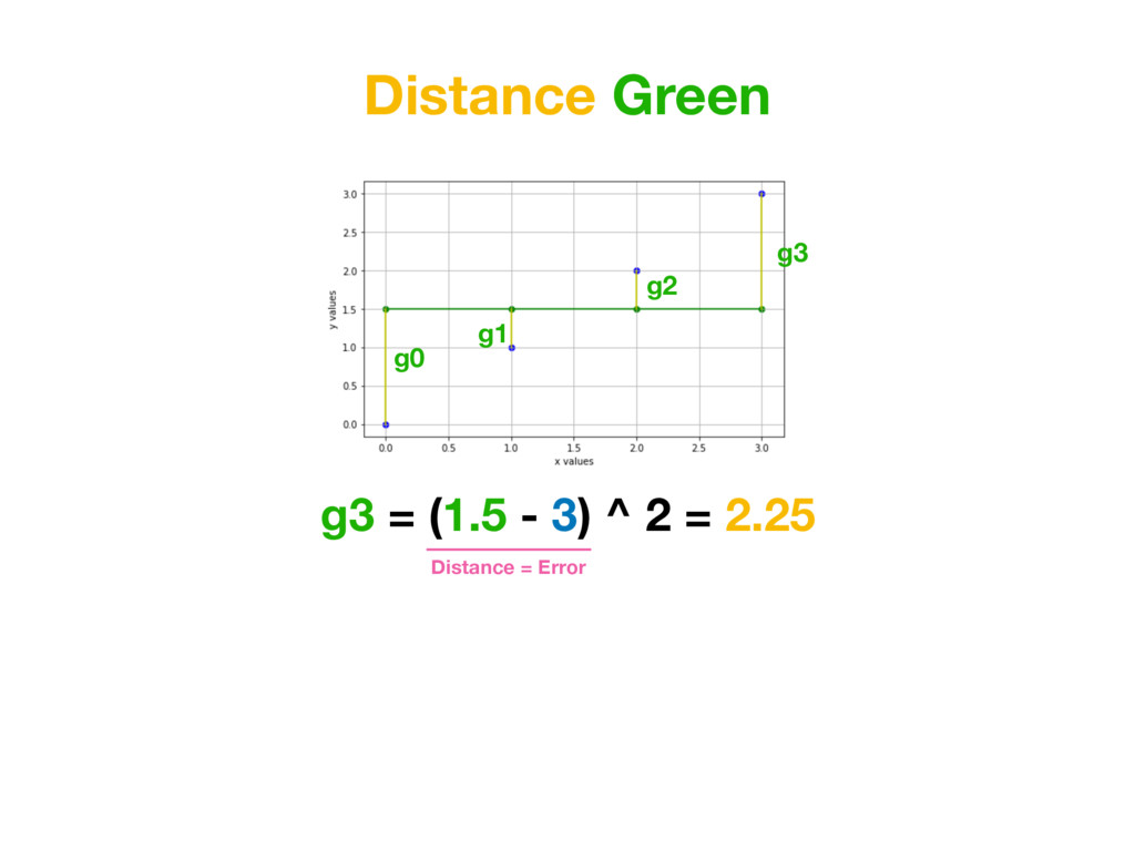
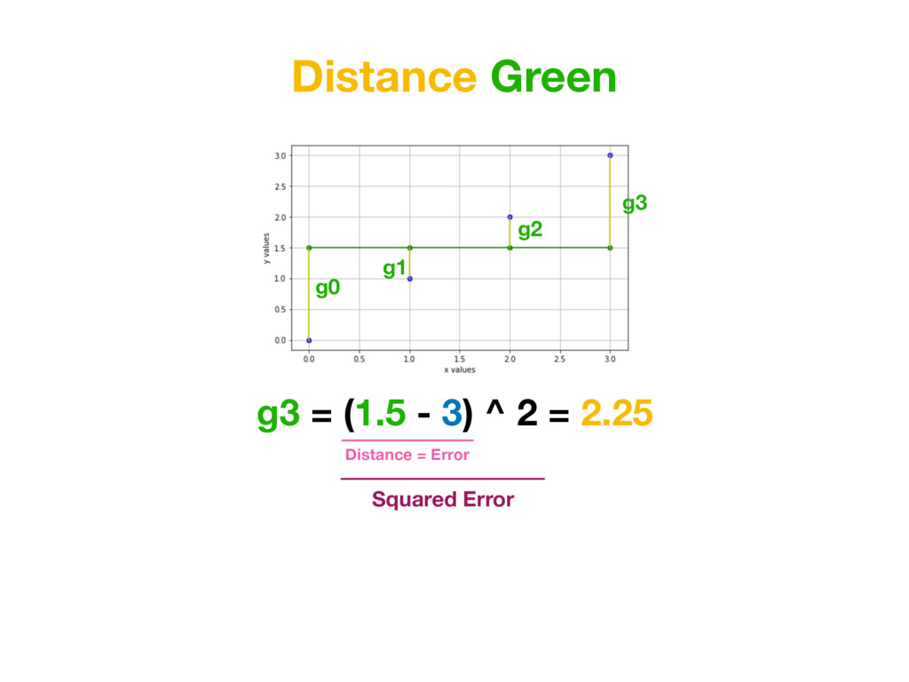
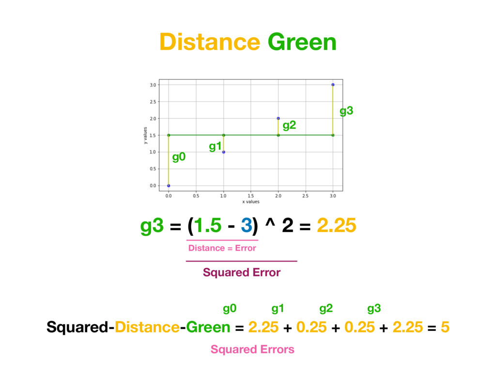
26. r0 r1 r2 r3 Distance Red 0 0 0 1 1 0.5 2 2 1 3 3 1.5 x h(x) = 0.5x y r0 = (0 - 0)^2 = 0 r1 = (0.5 - 1)^2 = 0.25 r2 = (1 - 2)^2 = 1 r3 = (1.5 - 3)^2 = 2.25 But additional thing we could do is to penalise distances which are too big more. To achieve that we simply need to square each value. (In Machine Learning world it’s called L2 Distance)
27. r0 r1 r2 r3 Distance Red 0 0 0 1 1 0.5 2 2 1 3 3 1.5 x h(x) = 0.5x y r0 = (0 - 0)^2 = 0 r1 = (0.5 - 1)^2 = 0.25 r2 = (1 - 2)^2 = 1 r3 = (1.5 - 3)^2 = 2.25 Squared-Distance-Red = 0 + 0.25 + 1 + 2.25 = 3.5
28. r0 r1 r2 r3 Distance Red 0 0 0 1 1 0.5 2 2 1 3 3 1.5 x h(x) = 0.5x y r0 = (0 - 0)^2 = 0 r1 = (0.5 - 1)^2 = 0.25 r2 = (1 - 2)^2 = 1 r3 = (1.5 - 3)^2 = 2.25 Squared-Distance-Red = 0 + 0.25 + 1 + 2.25 = 3.5 Average Distance = (0 + 0.25 + 1 + 2.25) / 4 = 0.875
29. Distance Green 0 0 1.5 1 1 1.5 2 2 1.5 3 3 1.5 x h(x) = 1.5 y g0 = (1.5 - 0)^2 = 2.25 g1 = (1.5 - 1)^2 = 0.25 g2 = (1.5 - 2)^2 = 0.25 g3 = (1.5 - 3)^2 = 2.25 Squared-Distance-Green = 2.25 + 0.25 + 0.25 + 2.25 = 5 Average Distance = (2.25 + 0.25 + 0.25 + 2.25) / 4 = 1.25 g0 g1 g2 g3
30. We can compare now! Average Distance Green = 1.25 Average Distance Red = 0.875 (Average Distance Red) < (Average Distance Green ) Function parameters a=0.5, b=0 are better than a=0, b=1.5…
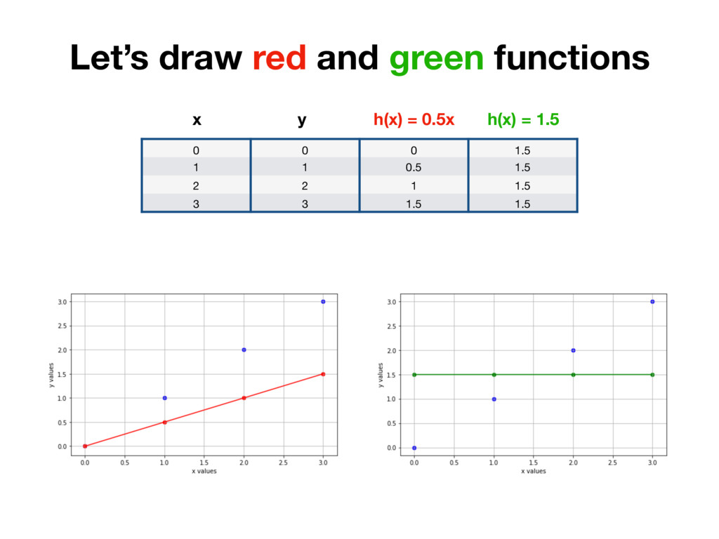
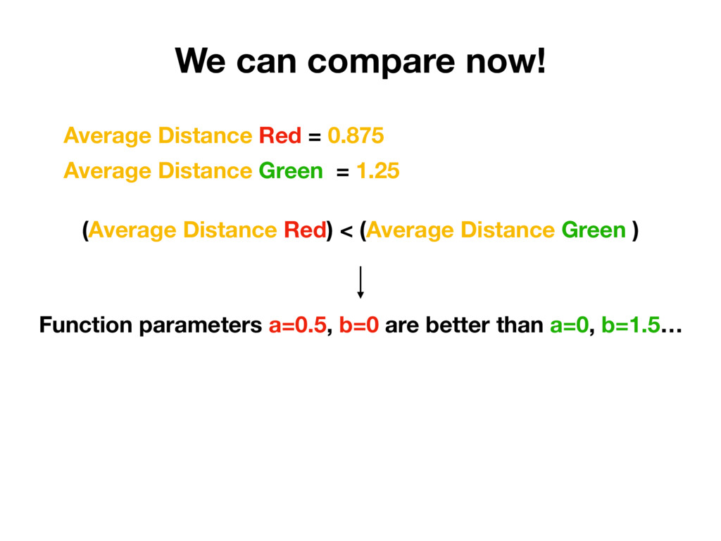
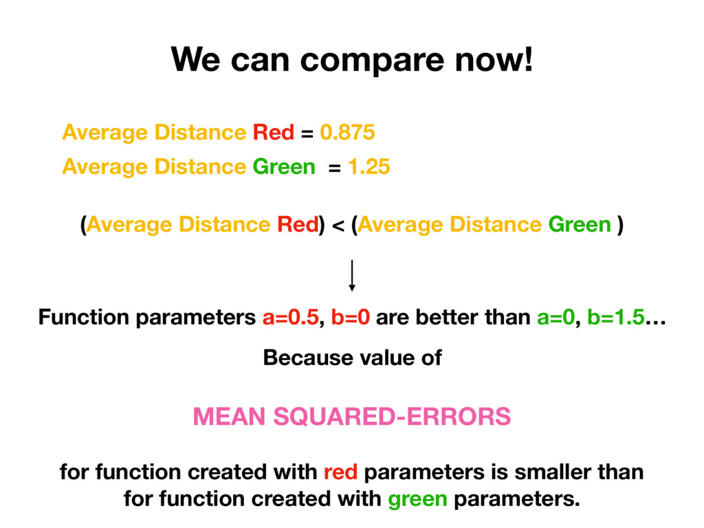
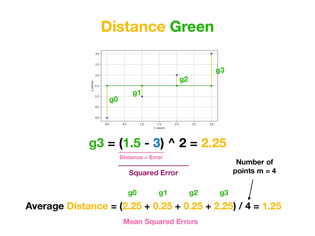
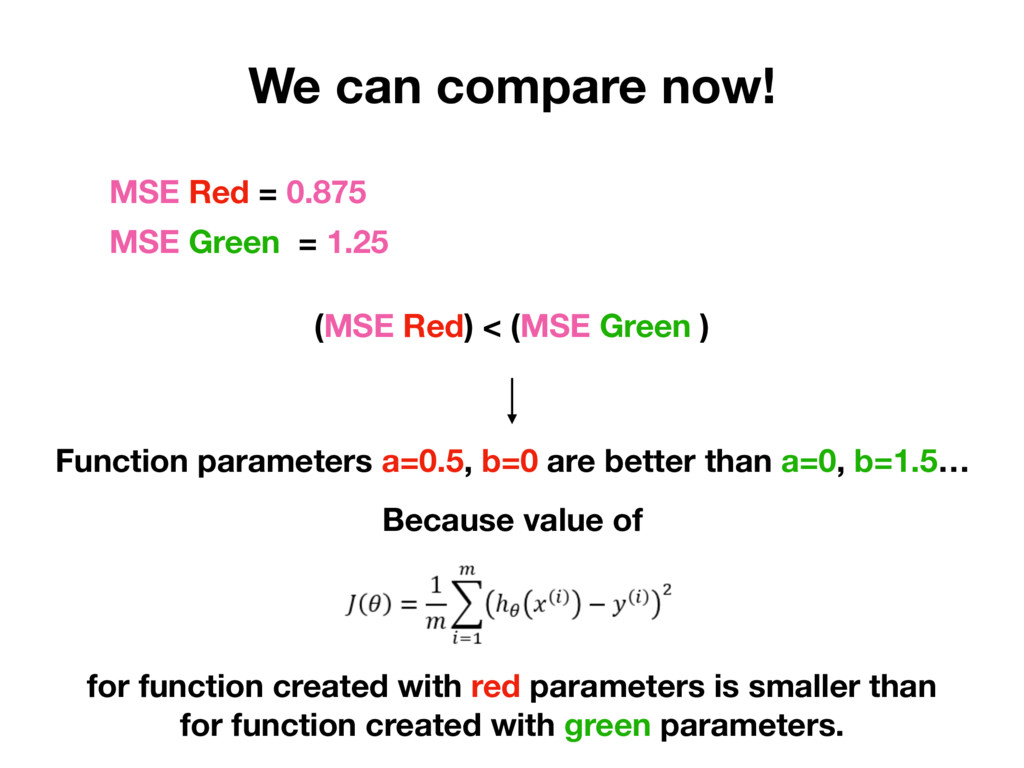
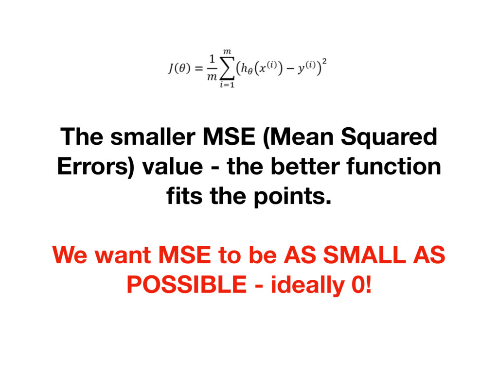
31. We can compare now! Function parameters a=0.5, b=0 are better than a=0, b=1.5… Because value of MEAN SQUARED-ERRORS for function created with red parameters is smaller than for function created with green parameters. Average Distance Green = 1.25 Average Distance Red = 0.875 (Average Distance Red) < (Average Distance Green )
32. Distance Green g0 g1 g2 g3 g3 = (1.5 - 3) ^ 2 = 2.25
33. Distance Green g0 g1 g2 g3 g3 = (1.5 - 3) ^ 2 = 2.25 Distance = Error
34. Distance Green g0 g1 g2 g3 g3 = (1.5 - 3) ^ 2 = 2.25 Distance = Error Squared Error
35. Distance Green g0 g1 g2 g3 g3 = (1.5 - 3) ^ 2 = 2.25 Distance = Error Squared Error g0 g1 g2 g3 Squared-Distance-Green = 2.25 + 0.25 + 0.25 + 2.25 = 5 Squared Errors
36. Distance Green g0 g1 g2 g3 g3 = (1.5 - 3) ^ 2 = 2.25 Distance = Error Squared Error g0 g1 g2 g3 Mean Squared Errors Average Distance = (2.25 + 0.25 + 0.25 + 2.25) / 4 = 1.25 Number of points m = 4
37. We can compare now! Function parameters a=0.5, b=0 are better than a=0, b=1.5… Because value of for function created with red parameters is smaller than for function created with green parameters. MSE Green = 1.25 MSE Red = 0.875 (MSE Red) < (MSE Green )
38. Let’s see how parameter a of function h(x) -> y = a * x affects value of MSE (Mean Squared Error). We ignore b parameter for simplification.
39. 0 0 1 1 2 2 3 3 x y
40. 0 0 1 1 2 2 3 3 x y Let’s pick large a = 10 and calculate MSE for given x, y:
41. 0 0 1 1 2 2 3 3 x y Let’s pick large a = 10 and calculate MSE for given x, y: h(x) = a * x m = 4 (because 4y values)
42. 0 0 1 1 2 2 3 3 x y Let’s pick large a = 10 and calculate MSE for given x, y: h(x) = a * x m = 4 (because 4y values)
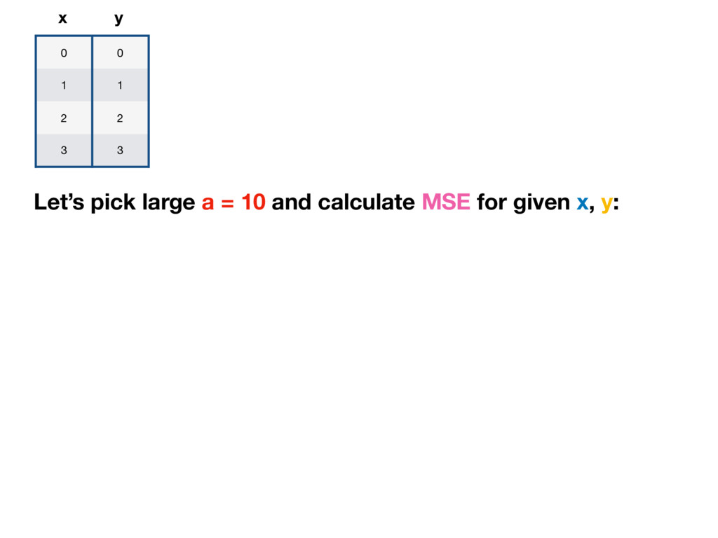
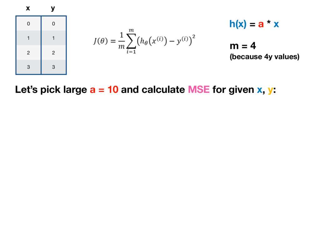
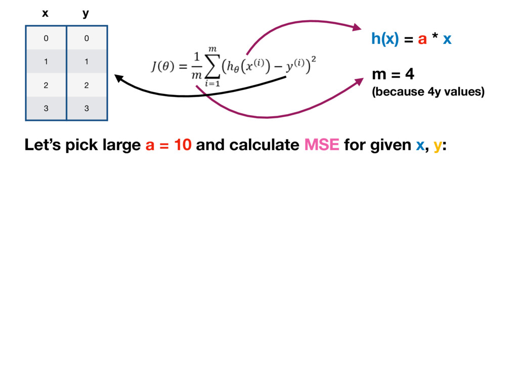
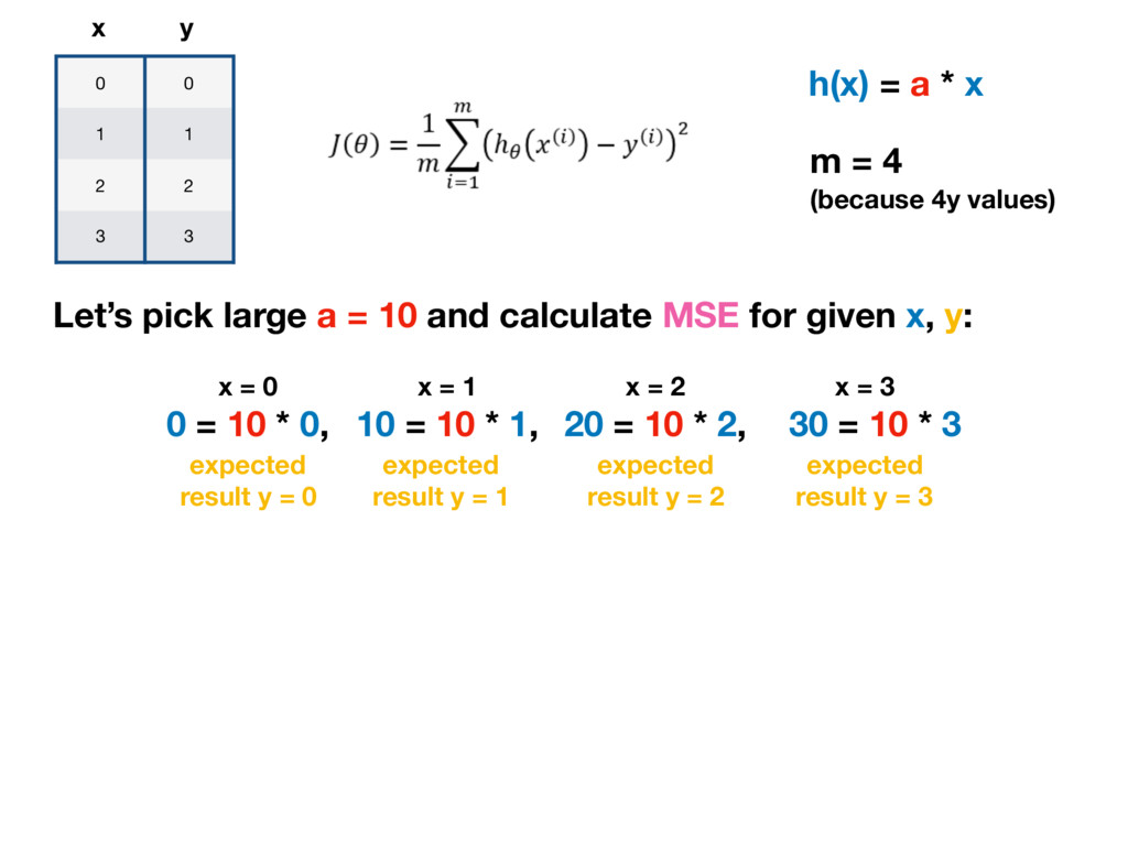
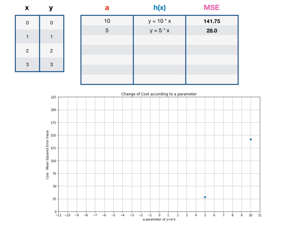
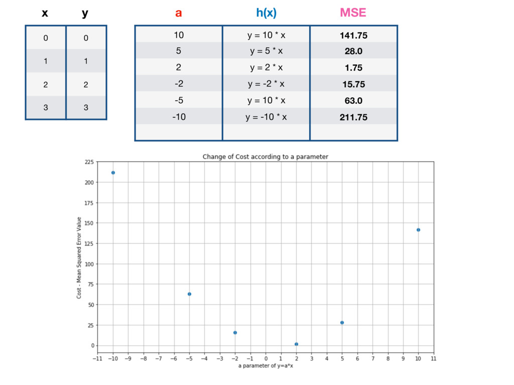
43. 0 0 1 1 2 2 3 3 x y h(x) = a * x m = 4 (because 4y values) Let’s pick large a = 10 and calculate MSE for given x, y: 0 = 10 * 0, x = 0 10 = 10 * 1, x = 1 20 = 10 * 2, x = 2 30 = 10 * 3 x = 3 expected result y = 0 expected result y = 1 expected result y = 2 expected result y = 3
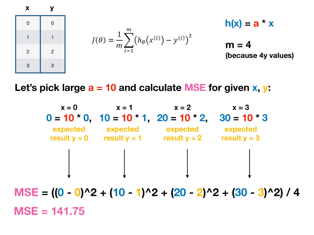
44. 0 0 1 1 2 2 3 3 x y Let’s pick large a = 10 and calculate MSE for given x, y: h(x) = a * x 0 = 10 * 0, m = 4 (because 4y values) x = 0 10 = 10 * 1, x = 1 20 = 10 * 2, x = 2 30 = 10 * 3 x = 3 expected result y = 0 expected result y = 1 expected result y = 2 expected result y = 3 MSE = ((0 - 0)^2 + (10 - 1)^2 + (20 - 2)^2 + (30 - 3)^2) / 4 MSE = 141.75
45. 0 0 1 1 2 2 3 3 x y 10 y = 10 * x 141.75 a h(x) MSE
46. 0 0 1 1 2 2 3 3 x y 10 y = 10 * x 141.75 5 y = 5 * x 28.0 a h(x) MSE
47. 0 0 1 1 2 2 3 3 x y 10 y = 10 * x 141.75 5 y = 5 * x 28.0 2 y = 2 * x 1.75 a h(x) MSE
48. 0 0 1 1 2 2 3 3 x y 10 y = 10 * x 141.75 5 y = 5 * x 28.0 2 y = 2 * x 1.75 -2 y = -2 * x 15.75 a h(x) MSE
49. 0 0 1 1 2 2 3 3 x y 10 y = 10 * x 141.75 5 y = 5 * x 28.0 2 y = 2 * x 1.75 -2 y = -2 * x 15.75 -5 y = 10 * x 63.0 a h(x) MSE
50. 0 0 1 1 2 2 3 3 x y 10 y = 10 * x 141.75 5 y = 5 * x 28.0 2 y = 2 * x 1.75 -2 y = -2 * x 15.75 -5 y = 10 * x 63.0 -10 y = -10 * x 211.75 a h(x) MSE
51. 0 0 1 1 2 2 3 3 x y 10 y = 10 * x 141.75 5 y = 5 * x 28.0 2 y = 2 * x 1.75 -2 y = -2 * x 15.75 -5 y = 10 * x 63.0 -10 y = -10 * x 211.75 1 y = x 0 a h(x) MSE
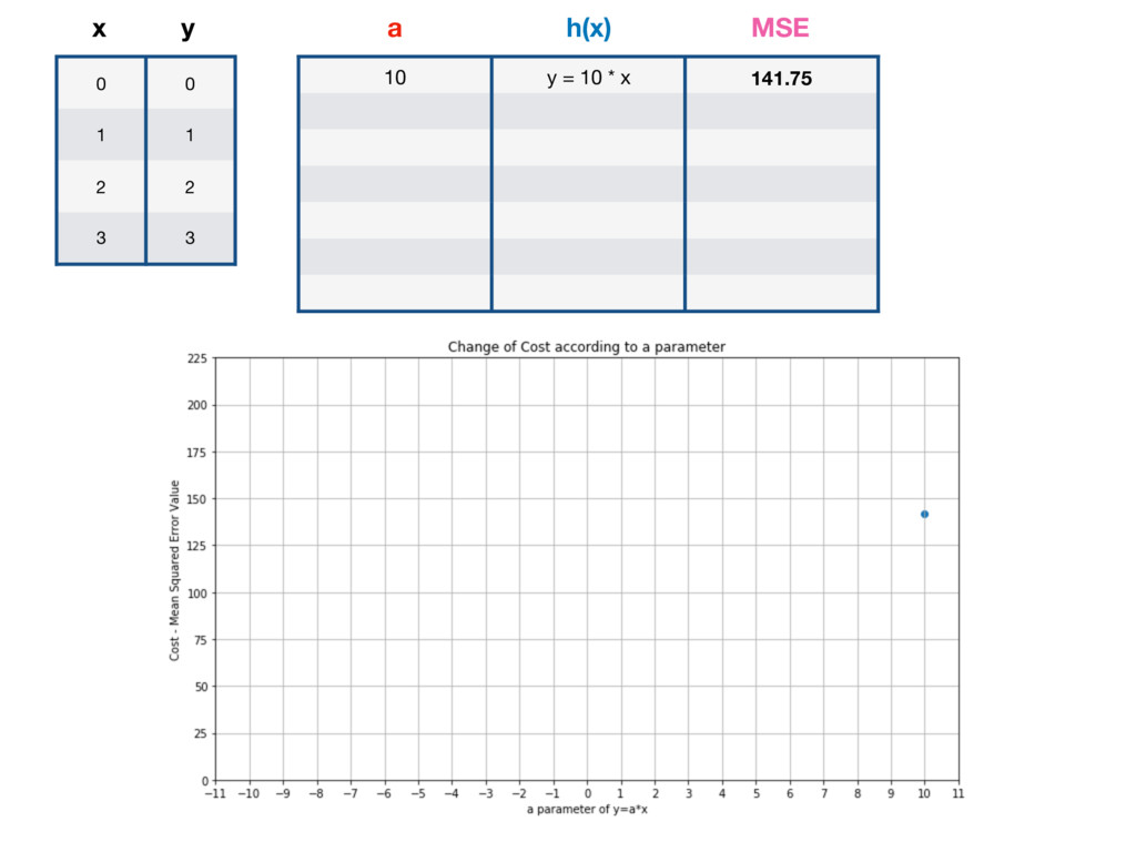
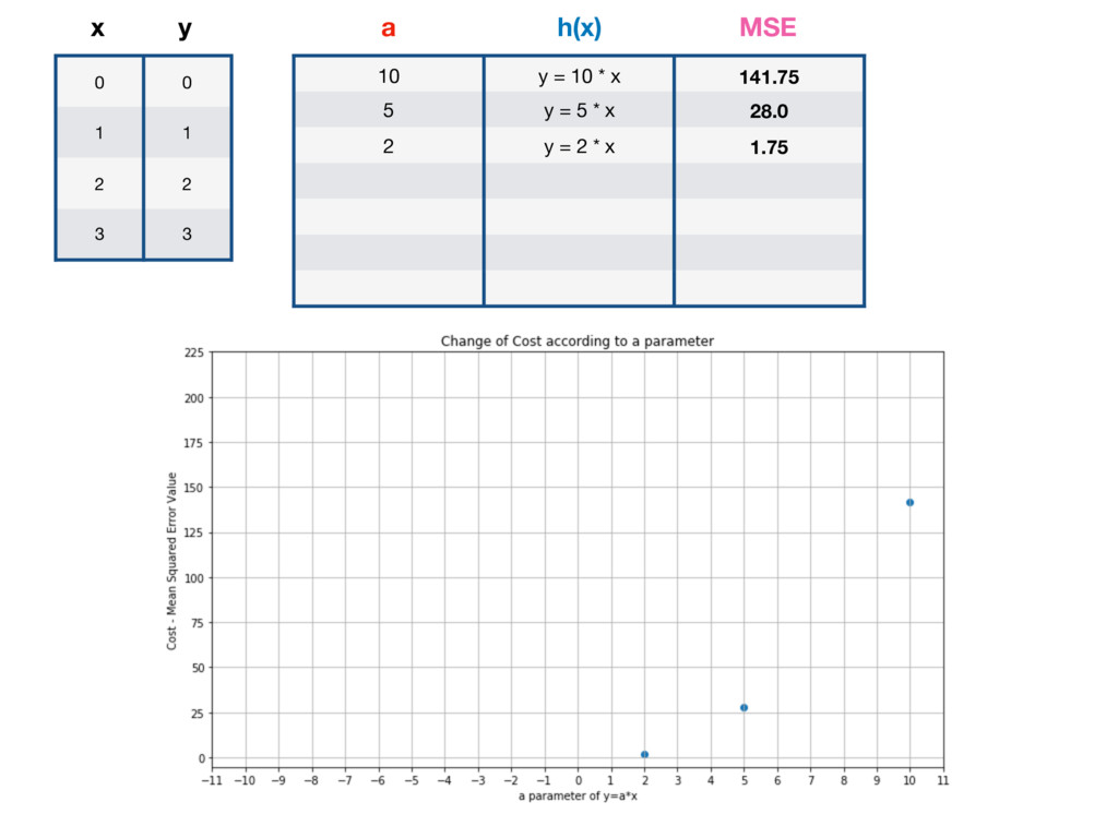
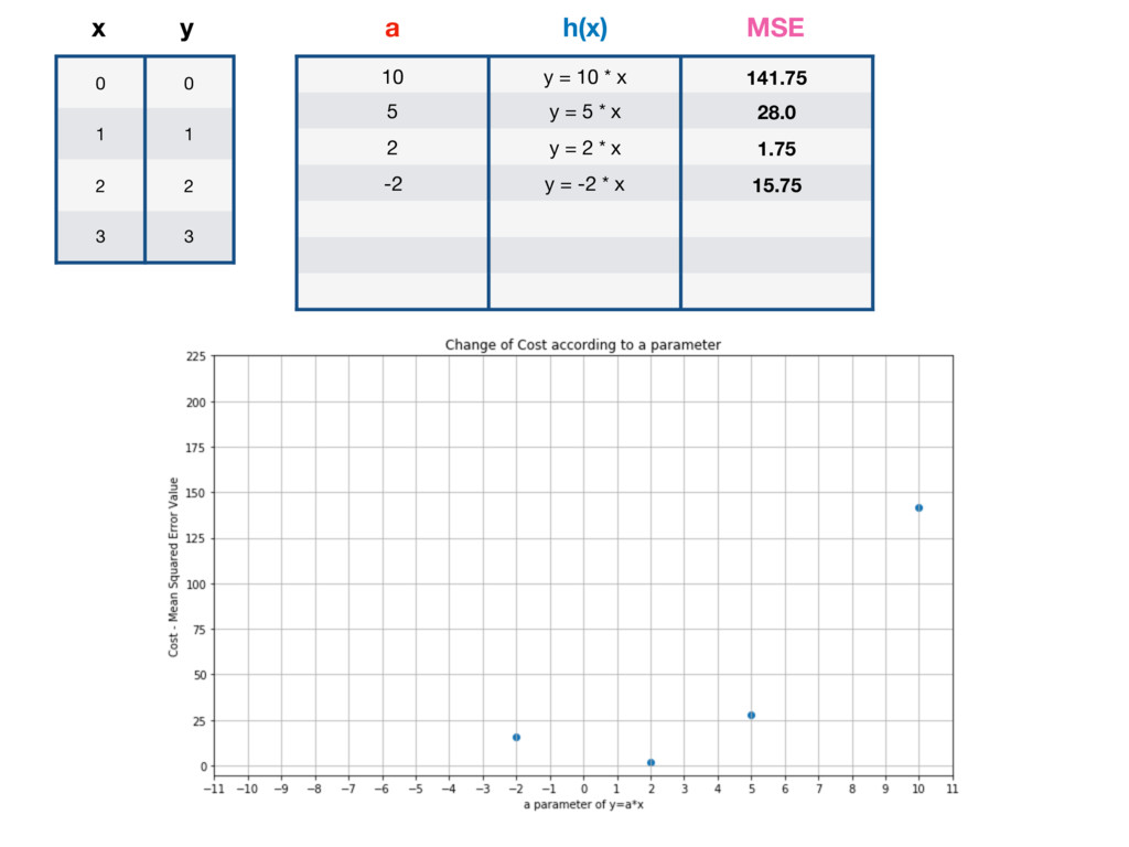
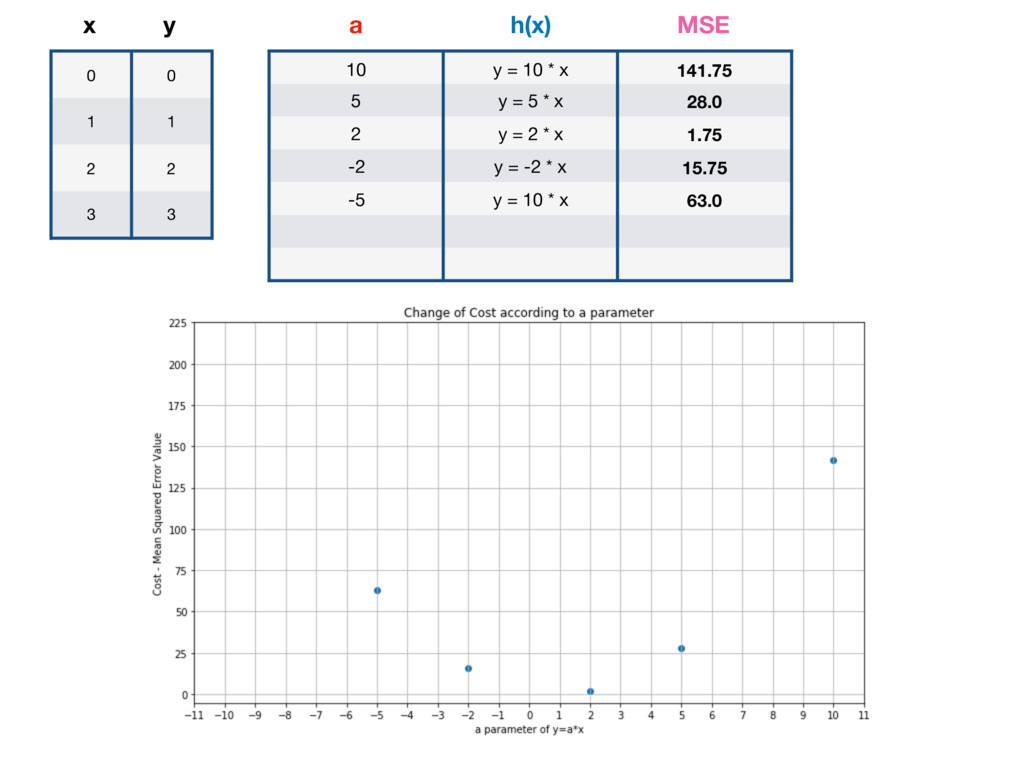
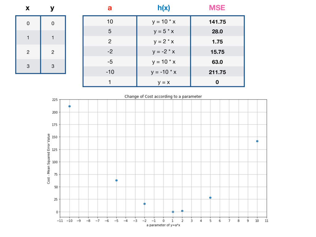
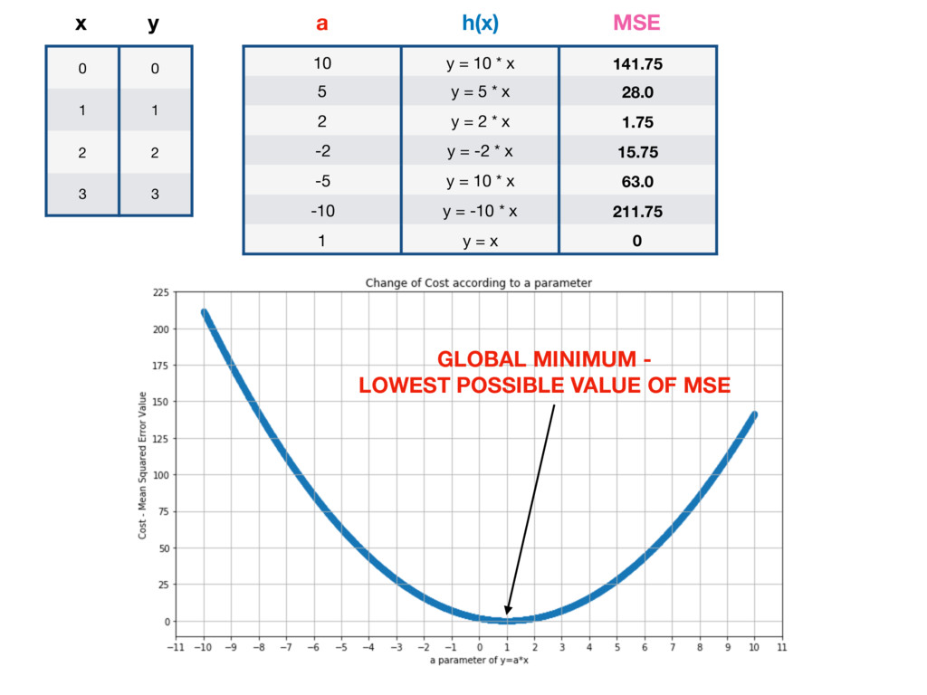
52. 0 0 1 1 2 2 3 3 x y 10 y = 10 * x 141.75 5 y = 5 * x 28.0 2 y = 2 * x 1.75 -2 y = -2 * x 15.75 -5 y = 10 * x 63.0 -10 y = -10 * x 211.75 1 y = x 0 a h(x) MSE GLOBAL MINIMUM - LOWEST POSSIBLE VALUE OF MSE
53. 0 0 1 1 2 2 3 3 x y 10 y = 10 * x 141.75 5 y = 5 * x 28.0 2 y = 2 * x 1.75 -2 y = -2 * x 15.75 -5 y = 10 * x 63.0 -10 y = -10 * x 211.75 1 y = x 0 a h(x) MSE y = 1 * x
54. The smaller MSE (Mean Squared Errors) value - the better function fits the points. We want MSE to be AS SMALL AS POSSIBLE - ideally 0!
55. It is possible to search for best h(x) parameters by randomly testing many different parameters and picking the one for which MSE is the lowest.
56. It is possible to search for best h(x) parameters by randomly testing many different parameters and picking the one for which MSE is the lowest. BUT IT'S INEFFICIENT!
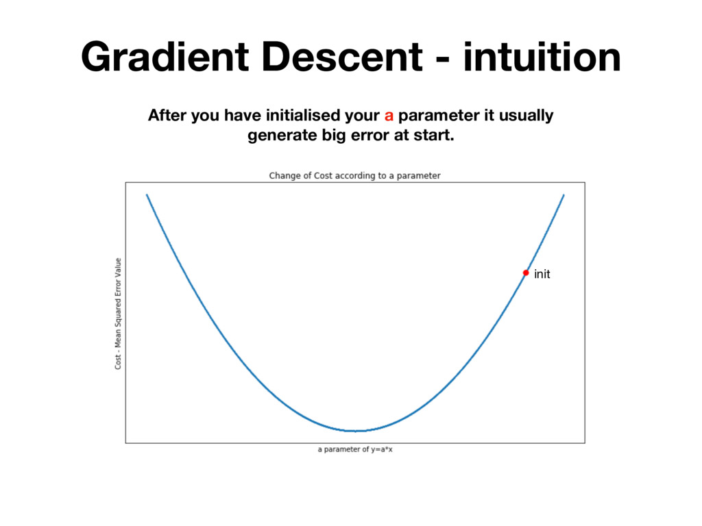
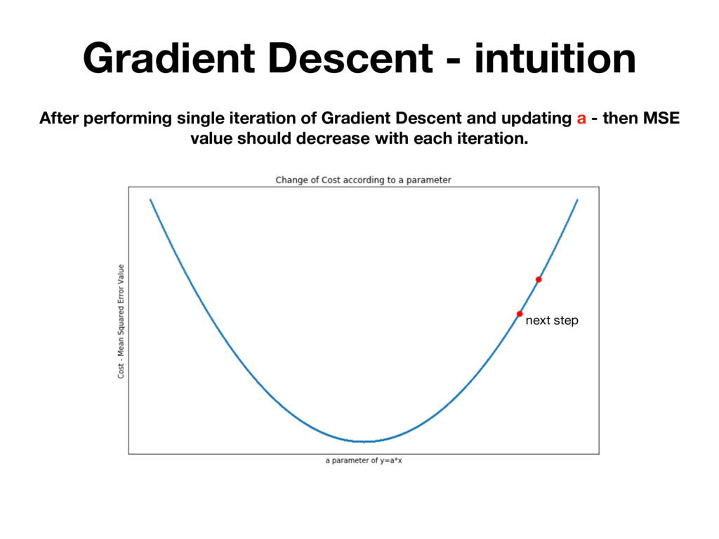
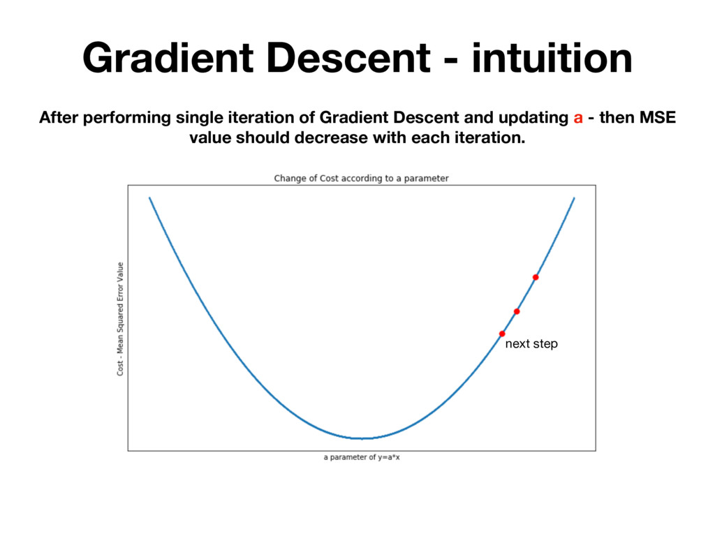
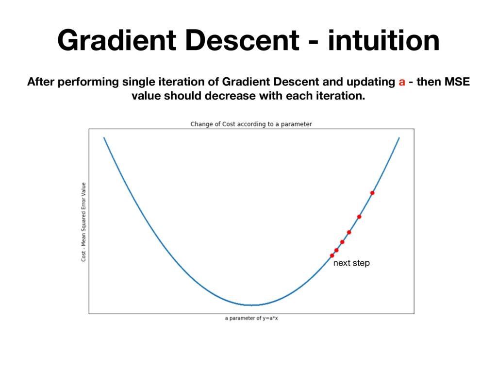
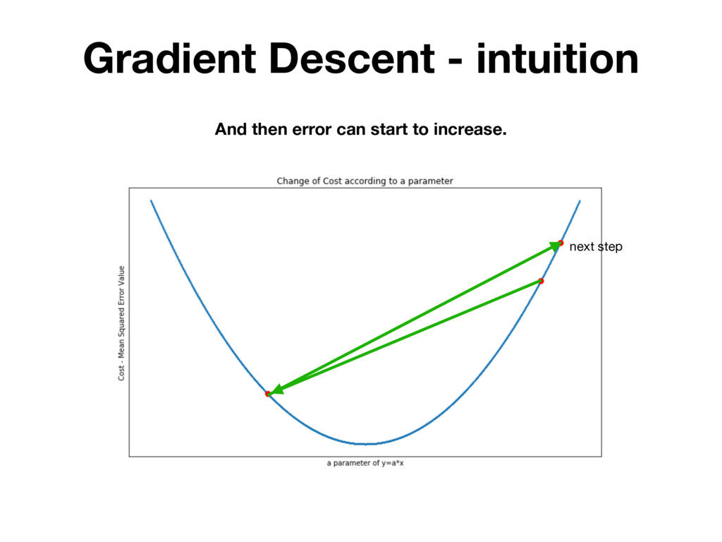
57. It is possible to search for best h(x) parameters by randomly testing many different parameters and picking the one for which MSE is the lowest. BUT IT'S INEFFICIENT! There is a mathematical method that allows you to change h(x) parameters in many iterations. Which each iteration MSE value is getting closer to it’s local minimum.
58. Gradient Descent Method for adjusting parameters in order to minimise MSE
59. Gradient Descent - recipe It can be mathematically proven that it works. For now trust it the same way you trust that recipe in cookbook won’t hurt your stomach :)
60. Gradient Descent - recipe Step 1: Decide on what function h(x) you want to find h(x) = a * x + b parameters to find: a, b
61. Gradient Descent - recipe Step 1: Decide on what function h(x) you want to find h(x) = a * x + b parameters to find: a, b Step 2: Decide on function that measures efficiency of h(x) Mean Squared Errors the lower value the better a, b parameters
62. Gradient Descent - recipe Step 1: Decide on what function h(x) you want to find h(x) = a * x + b parameters to find: a, b Step 2: Decide on function that measures efficiency of h(x) Mean Squared Errors the lower value the better a, b parameters Step 3: Take derivatives of MSE in respect to a, b dMSE(h(x), y) da = dMSE(h(x), y) db =
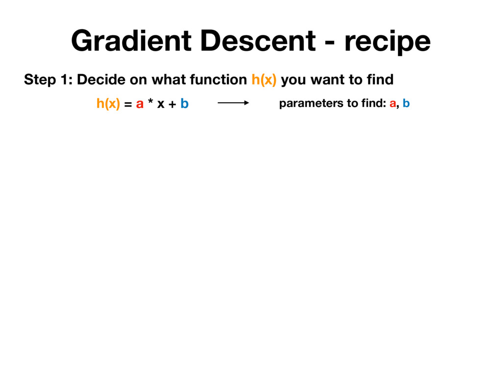
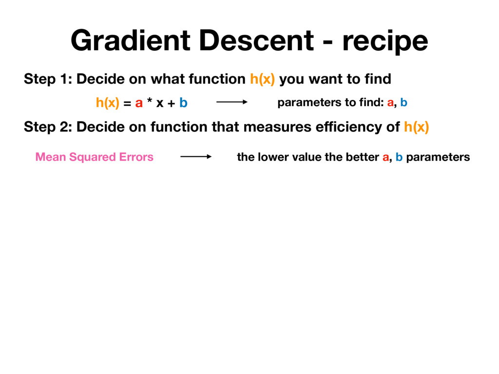
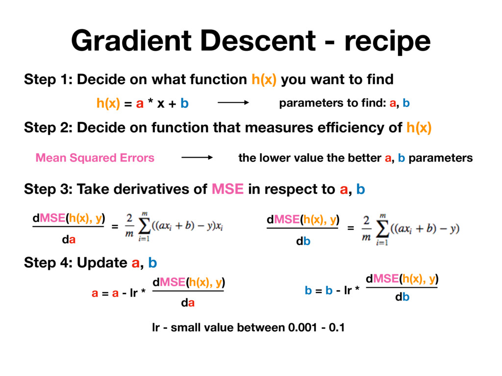
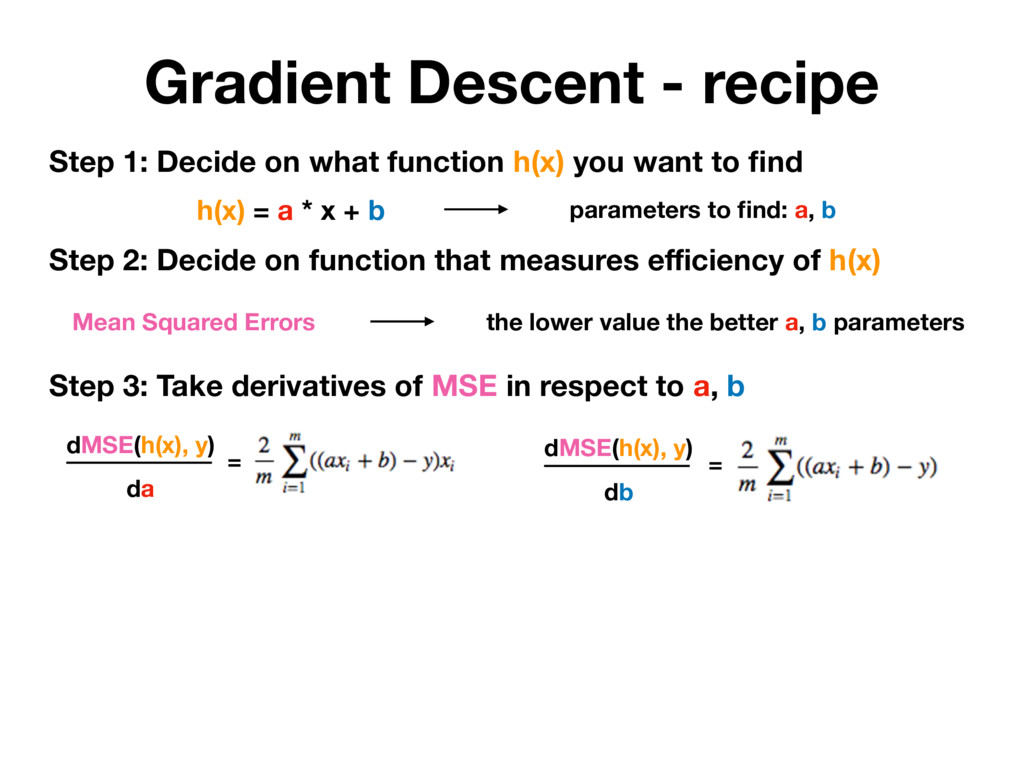
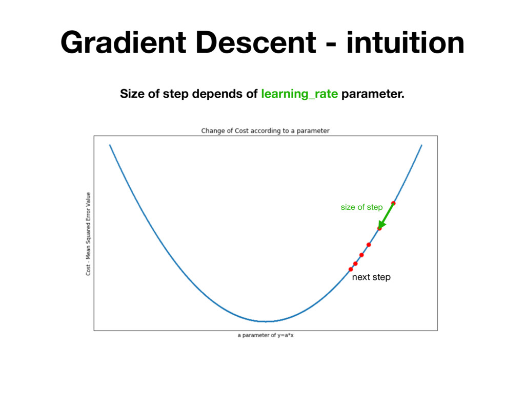
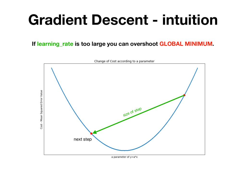
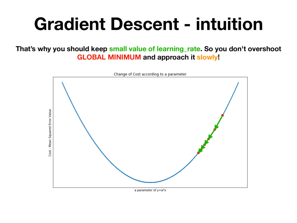
63. Gradient Descent - recipe Step 1: Decide on what function h(x) you want to find h(x) = a * x + b parameters to find: a, b Step 2: Decide on function that measures efficiency of h(x) Mean Squared Errors the lower value the better a, b parameters Step 3: Take derivatives of MSE in respect to a, b dMSE(h(x), y) da = dMSE(h(x), y) db = Step 4: Update a, b a = a - lr * b = b - lr * dMSE(h(x), y) da dMSE(h(x), y) db lr - small value between 0.001 - 0.1
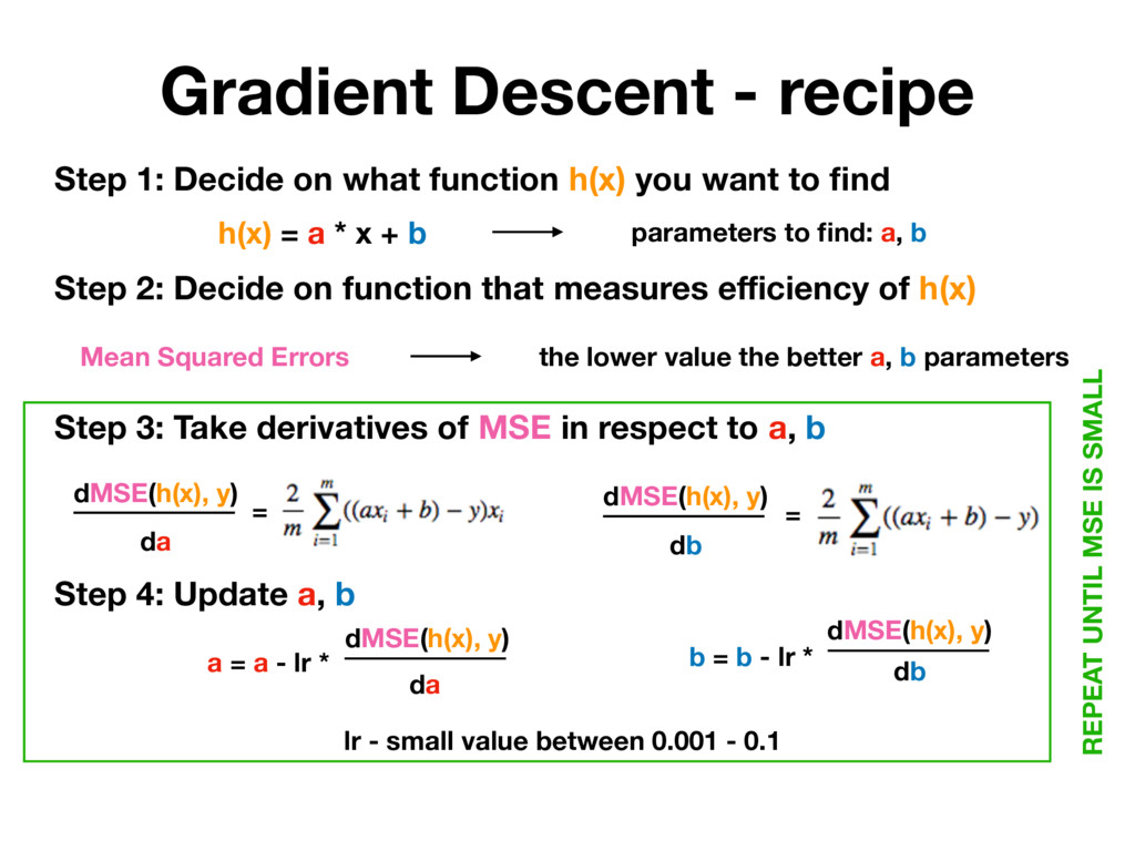
64. Gradient Descent - recipe Step 1: Decide on what function h(x) you want to find h(x) = a * x + b parameters to find: a, b Step 2: Decide on function that measures efficiency of h(x) Mean Squared Errors the lower value the better a, b parameters Step 3: Take derivatives of MSE in respect to a, b dMSE(h(x), y) da = dMSE(h(x), y) db = Step 4: Update a, b a = a - lr * b = b - lr * dMSE(h(x), y) da dMSE(h(x), y) db lr - small value between 0.001 - 0.1 REPEAT UNTIL MSE IS SMALL
65. Gradient Descent - intuition After you have initialised your a parameter it usually generate big error at start. init
66. Gradient Descent - intuition After performing single iteration of Gradient Descent and updating a - then MSE value should decrease with each iteration. next step
67. Gradient Descent - intuition After performing single iteration of Gradient Descent and updating a - then MSE value should decrease with each iteration. next step
68. Gradient Descent - intuition After performing single iteration of Gradient Descent and updating a - then MSE value should decrease with each iteration. next step
69. Gradient Descent - intuition After performing single iteration of Gradient Descent and updating a - then MSE value should decrease with each iteration. step 3 next step
70. Gradient Descent - intuition After performing single iteration of Gradient Descent and updating a - then MSE value should decrease with each iteration. step 3 next step
71. Gradient Descent - intuition Size of step depends of learning_rate parameter. step 3 next step size of step
72. Gradient Descent - intuition If learning_rate is too large you can overshoot GLOBAL MINIMUM. next step size of step
73. Gradient Descent - intuition And then error can start to increase. next step next step
74. Gradient Descent - intuition That’s why you should keep small value of learning_rate. So you don't overshoot GLOBAL MINIMUM and approach it slowly! step 3
75. After implementing this in code we can solve our problem (visualisation part - running coded theory in Python and showing how graph changes)