Upgrade to Pro — share decks privately, control downloads, hide ads and more …

urbcomp_ppt_v5.pdf

Sponsored · Your Podcast. Everywhere. Effortlessly. Share. Educate. Inspire. Entertain. You do you. We'll handle the rest. →
Avatar for gunjanthesystem gunjanthesystem
August 08, 2016
2

 urbcomp_ppt_v5.pdf

Avatar for gunjanthesystem

gunjanthesystem

August 08, 2016

Transcript

  1. Personalised Recommendations for Modes of Transport: A Sequence-based Approach Gunjan

    Kumar, Houssem Jerbi, and Michael P. O’Mahony Insight Centre for Data Analytics University College Dublin, Ireland UrbComp ‘16, San Francisco Aug 14, 2016
  2. Outline 1. Introduction 2. Recommendation Approach 3. Learning Personalised Optimal

    Matching Units 4. Evaluation 5. Conclusions and Future Work Insight Centre for Data Analytics UrbComp 2016 Slide 2
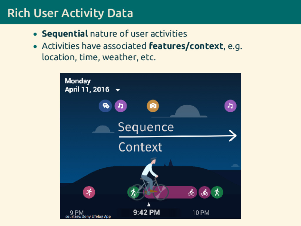
  3. Rich User Activity Data • Sequential nature of user activities

    • Activities have associated features/context, e.g. location, time, weather, etc.
  4. For Recommender Systems Facilitates real time recommendations for a given

    user and context (e.g. time, location, weather, etc.) Insight Centre for Data Analytics UrbComp 2016 Slide 5
  5. For Recommender Systems Facilitates real time recommendations for a given

    user and context (e.g. time, location, weather, etc.) Previous work: A framework for sequence- and context-based activity recommendation [Kumar et al., 2014] Insight Centre for Data Analytics UrbComp 2016 Slide 5
  6. For Recommender Systems Facilitates real time recommendations for a given

    user and context (e.g. time, location, weather, etc.) Previous work: A framework for sequence- and context-based activity recommendation [Kumar et al., 2014] Current Research Problem: Recommending the next mode of transport to users. Insight Centre for Data Analytics UrbComp 2016 Slide 5
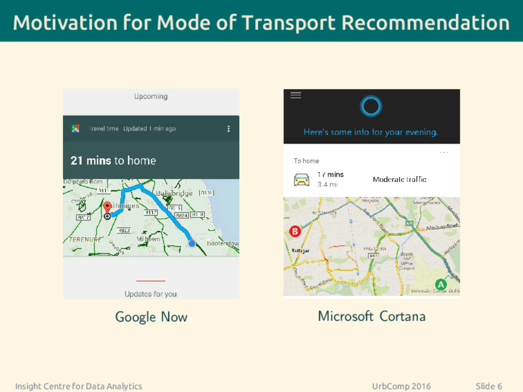
  7. Motivation for Mode of Transport Recommendation Google Now Microsoft Cortana

    Insight Centre for Data Analytics UrbComp 2016 Slide 6
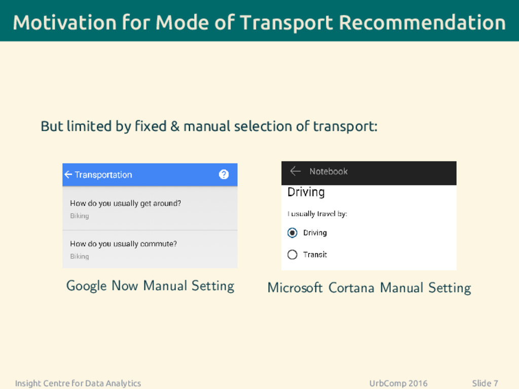
  8. Motivation for Mode of Transport Recommendation But limited by fixed

    & manual selection of transport: Google Now Manual Setting Microsoft Cortana Manual Setting Insight Centre for Data Analytics UrbComp 2016 Slide 7
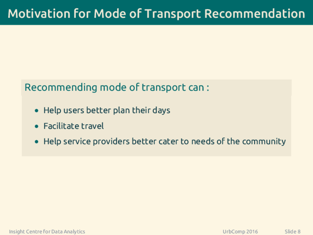
  9. Motivation for Mode of Transport Recommendation Recommending mode of transport

    can : • Help users better plan their days • Facilitate travel • Help service providers better cater to needs of the community Insight Centre for Data Analytics UrbComp 2016 Slide 8
  10. Related Work Capturing Sequence in UrbComp/RecSys • Hierarchical-graph-based model: •

    Mine popular travel sequences from location trajectories • Itinerary recommendation - [Li et al., 2008; Zheng et al., 2009; Yoon et al., 2010] • All-kth-order Markov models: • Webpage, music recommendation - [Bohnenberger and Jameson, 2001; Deshpande and Karypis, 2004; Shani et al., 2005]
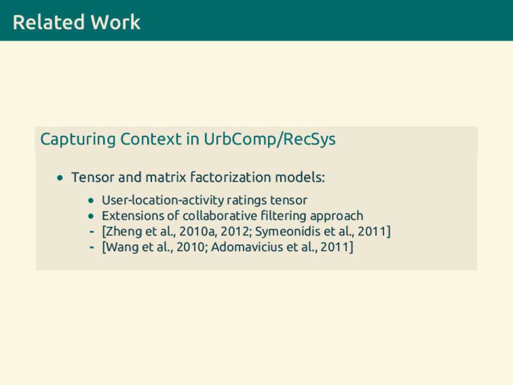
  11. Related Work Capturing Context in UrbComp/RecSys • Tensor and matrix

    factorization models: • User-location-activity ratings tensor • Extensions of collaborative filtering approach - [Zheng et al., 2010a, 2012; Symeonidis et al., 2011] - [Wang et al., 2010; Adomavicius et al., 2011]
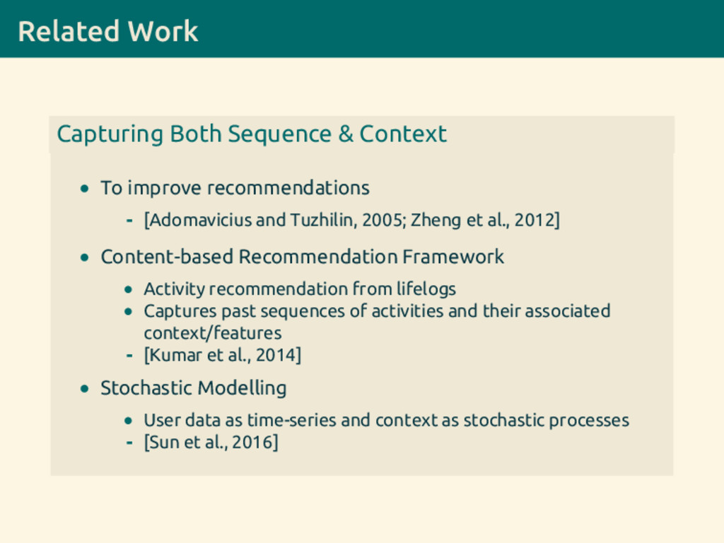
  12. Related Work Capturing Both Sequence & Context • To improve

    recommendations - [Adomavicius and Tuzhilin, 2005; Zheng et al., 2012] • Content-based Recommendation Framework • Activity recommendation from lifelogs • Captures past sequences of activities and their associated context/features - [Kumar et al., 2014] • Stochastic Modelling • User data as time-series and context as stochastic processes - [Sun et al., 2016]
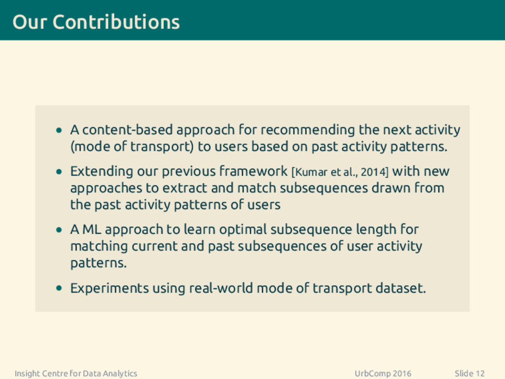
  13. Our Contributions • A content-based approach for recommending the next

    activity (mode of transport) to users based on past activity patterns. • Extending our previous framework [Kumar et al., 2014] with new approaches to extract and match subsequences drawn from the past activity patterns of users • A ML approach to learn optimal subsequence length for matching current and past subsequences of user activity patterns. • Experiments using real-world mode of transport dataset. Insight Centre for Data Analytics UrbComp 2016 Slide 12
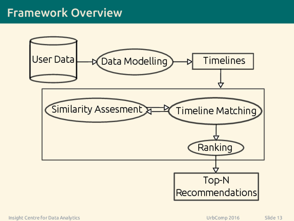
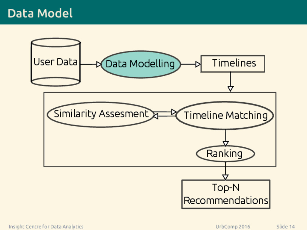
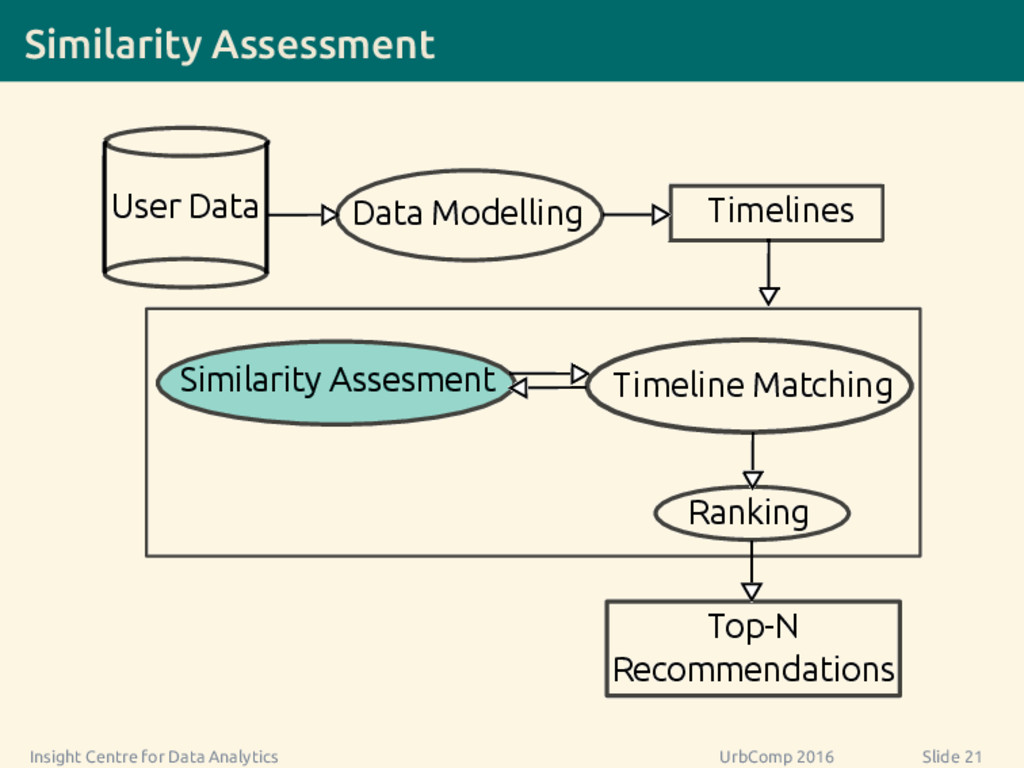
  14. Framework Overview Ranking User Data Timelines Data Modelling Timeline Matching

    Top-N Recommendations Similarity Assesment Insight Centre for Data Analytics UrbComp 2016 Slide 13
  15. Data Model Ranking User Data Timelines Data Modelling Timeline Matching

    Top-N Recommendations Similarity Assesment Insight Centre for Data Analytics UrbComp 2016 Slide 14
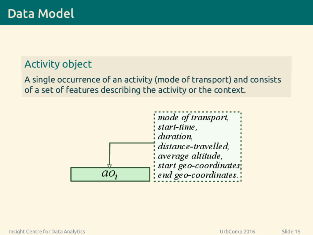
  16. Data Model Activity object A single occurrence of an activity

    (mode of transport) and consists of a set of features describing the activity or the context. mode of transport, start-time, duration, distance-travelled, average altitude, start geo-coordinates, end geo-coordinates. aoi Insight Centre for Data Analytics UrbComp 2016 Slide 15
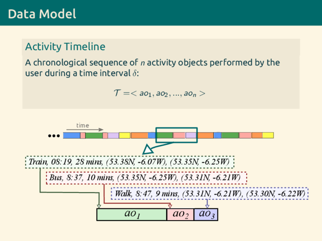
  17. Data Model Activity Timeline A chronological sequence of n activity

    objects performed by the user during a time interval δ: T =< ao1, ao2, ..., aon > time Train, 08:19, 28 mins, (53.38N, -6.07W), (53.35N, -6.25W) Walk, 8:47, 9 mins, (53.31N, -6.21W), (53.30N, -6.22W) Bus, 8:37, 10 mins, (53.35N, -6.25W), (53.31N, -6.21W) ao1 ao3
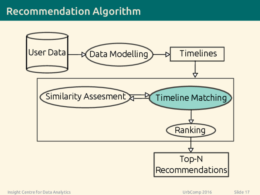
  18. Recommendation Algorithm Ranking User Data Timelines Data Modelling Timeline Matching

    Top-N Recommendations Similarity Assesment Insight Centre for Data Analytics UrbComp 2016 Slide 17
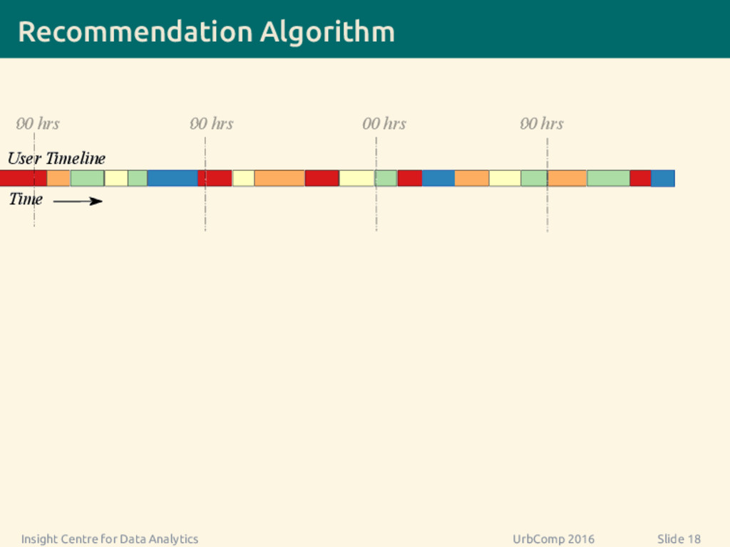
  19. Recommendation Algorithm User Timeline Time 00 hrs 00 hrs 00

    hrs 00 hrs Insight Centre for Data Analytics UrbComp 2016 Slide 18
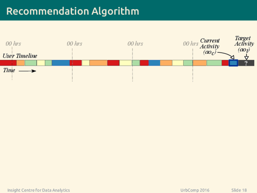
  20. Recommendation Algorithm Target Activity (aot) Current Activity (aoc) User Timeline

    Time ? 00 hrs 00 hrs 00 hrs 00 hrs Insight Centre for Data Analytics UrbComp 2016 Slide 18
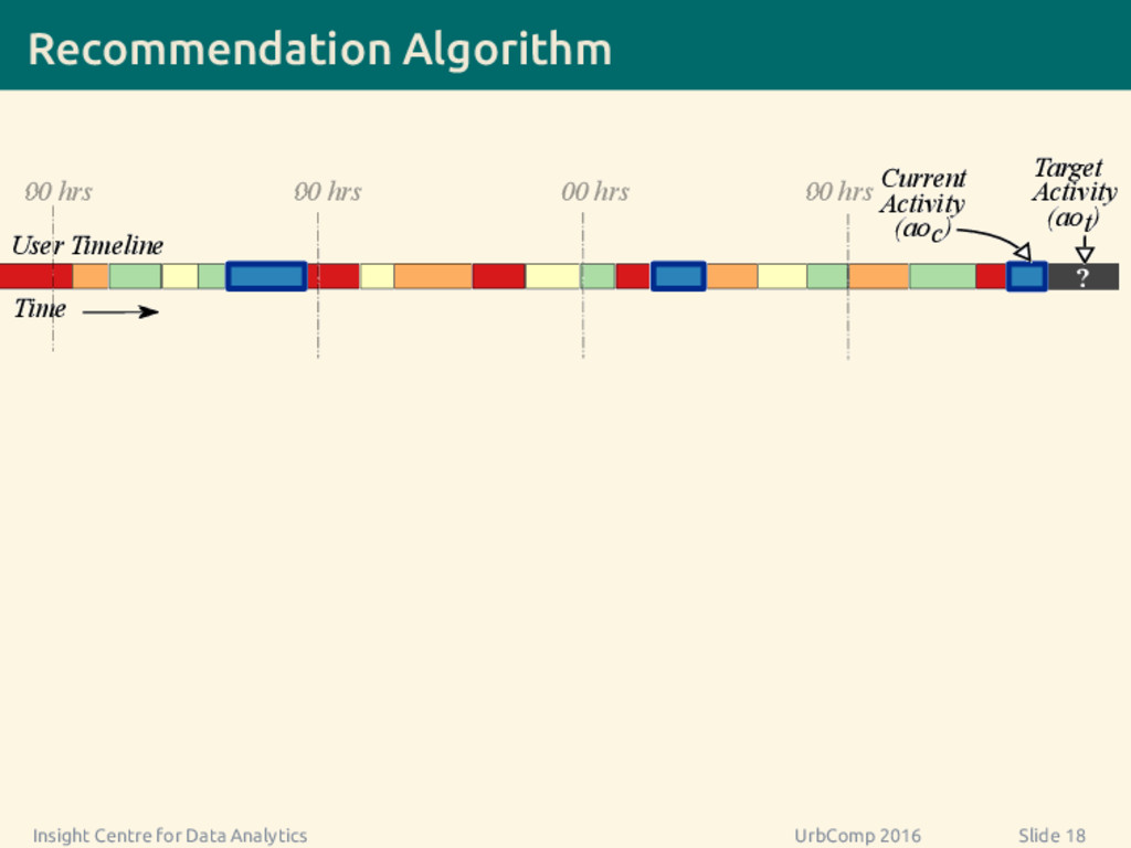
  21. Recommendation Algorithm Target Activity (aot) Current Activity (aoc) User Timeline

    Time ? 00 hrs 00 hrs 00 hrs 00 hrs Insight Centre for Data Analytics UrbComp 2016 Slide 18
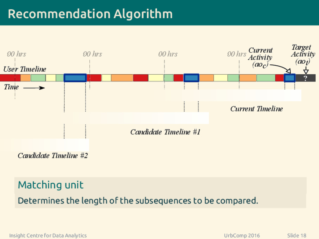
  22. Recommendation Algorithm Target Activity (aot) Current Activity (aoc) User Timeline

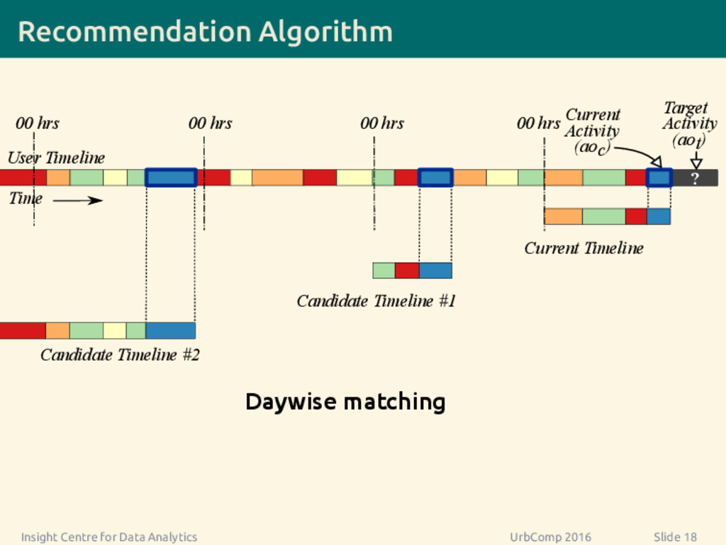
    Time ? 00 hrs 00 hrs 00 hrs 00 hrs Candidate Timeline #2 Candidate Timeline #1 Current Timeline Matching unit Determines the length of the subsequences to be compared. Insight Centre for Data Analytics UrbComp 2016 Slide 18
  23. Recommendation Algorithm Target Activity (aot) Current Activity (aoc) User Timeline

    Time ? 00 hrs 00 hrs 00 hrs 00 hrs Candidate Timeline #2 Candidate Timeline #1 Current Timeline Daywise matching Insight Centre for Data Analytics UrbComp 2016 Slide 18
  24. Recommendation Algorithm 4 3 2 1 4 3 2 1

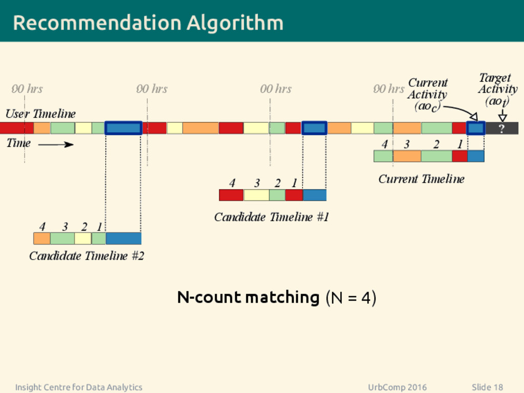
    4 3 2 1 N-count matching Target Activity (aot) Current Activity (aoc) User Timeline Time ? 00 hrs 00 hrs 00 hrs 00 hrs Candidate Timeline #2 Candidate Timeline #1 Current Timeline (N = 4) Insight Centre for Data Analytics UrbComp 2016 Slide 18
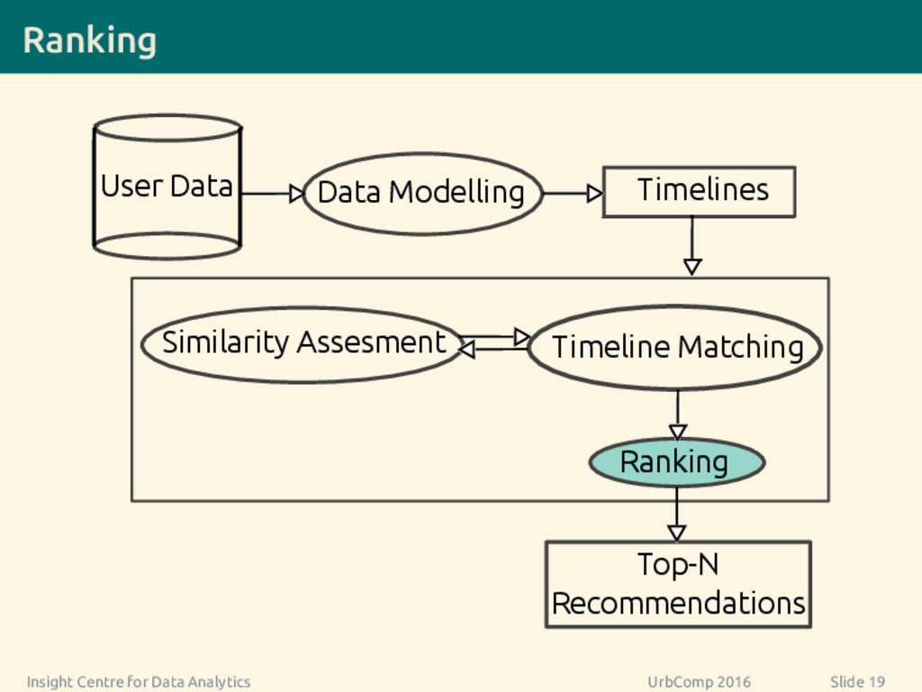
  25. Ranking Ranking User Data Timelines Data Modelling Timeline Matching Top-N

    Recommendations Similarity Assesment Insight Centre for Data Analytics UrbComp 2016 Slide 19
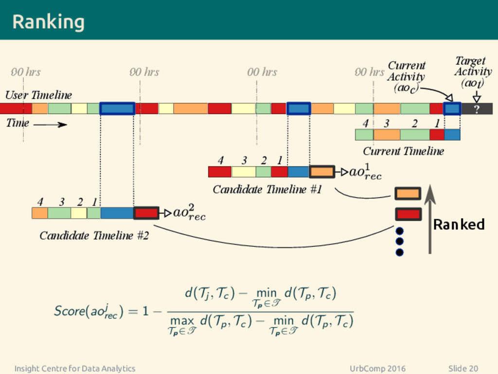
  26. Ranking 4 3 2 1 4 3 2 1 4

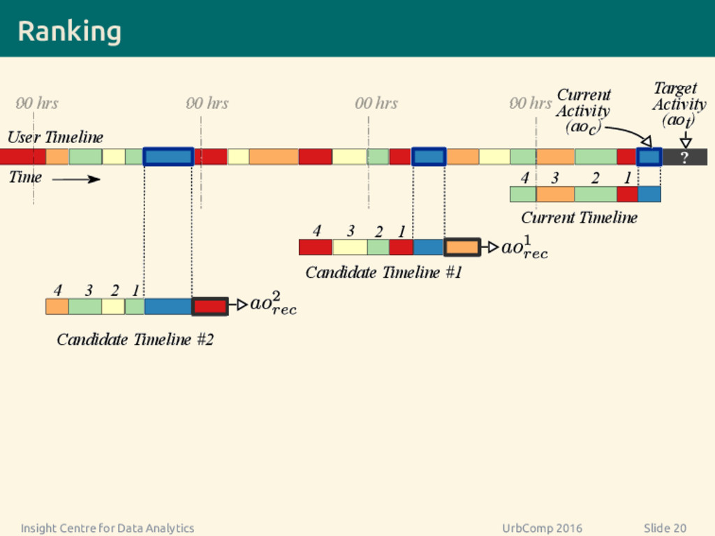
    3 2 1 Target Activity (aot) Current Activity (aoc) User Timeline Time ? 00 hrs 00 hrs 00 hrs 00 hrs Candidate Timeline #2 Candidate Timeline #1 Current Timeline Insight Centre for Data Analytics UrbComp 2016 Slide 20
  27. Ranking Ranked 4 3 2 1 4 3 2 1

    4 3 2 1 Target Activity (aot) Current Activity (aoc) User Timeline Time ? Candidate Timeline #2 Candidate Timeline #1 Current Timeline 00 hrs 00 hrs 00 hrs 00 hrs Score(aoj rec ) = 1 − d(Tj , Tc ) − min Tp∈T d(Tp, Tc ) max Tp∈T d(Tp, Tc ) − min Tp∈T d(Tp, Tc ) Insight Centre for Data Analytics UrbComp 2016 Slide 20
  28. Similarity Assessment Ranking User Data Timelines Data Modelling Timeline Matching

    Top-N Recommendations Similarity Assesment Insight Centre for Data Analytics UrbComp 2016 Slide 21
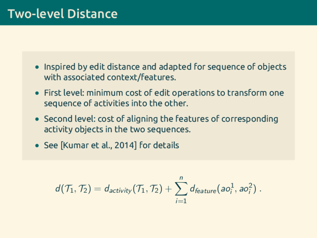
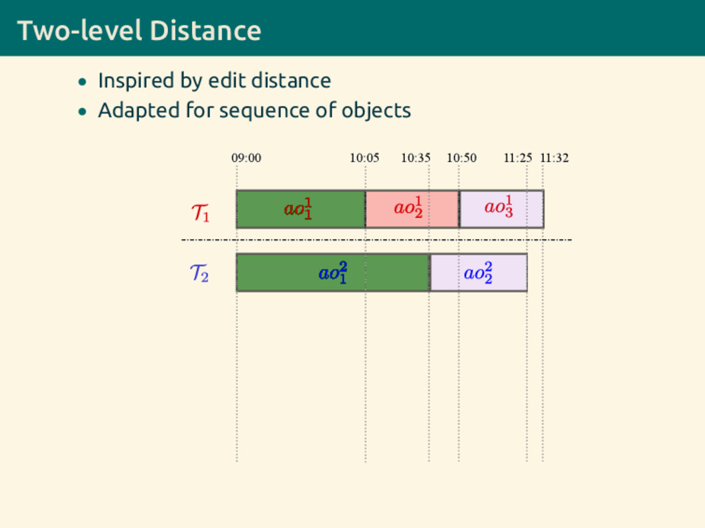
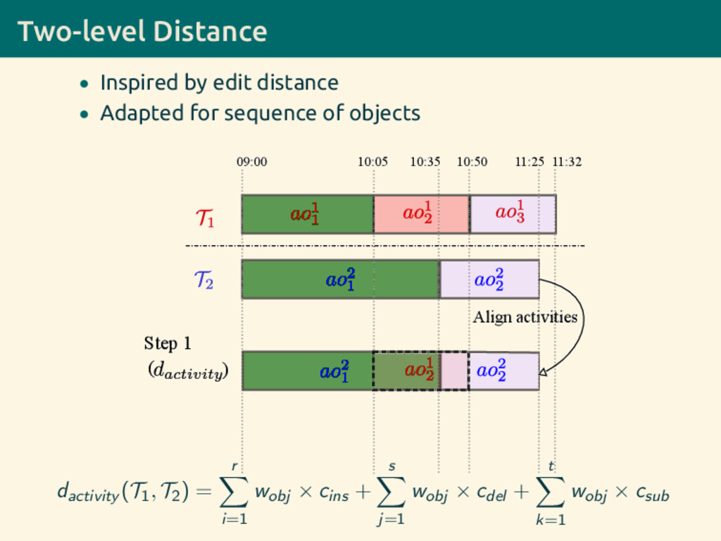
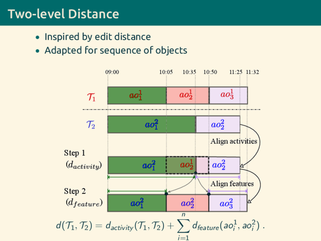
  29. Two-level Distance • Inspired by edit distance and adapted for

    sequence of objects with associated context/features. • First level: minimum cost of edit operations to transform one sequence of activities into the other. • Second level: cost of aligning the features of corresponding activity objects in the two sequences. • See [Kumar et al., 2014] for details d(T1, T2) = dactivity (T1, T2) + n i=1 dfeature(ao1 i , ao2 i ) .
  30. Learning Personalised Optimal Matching Units • Timeline Matching requires a

    matching unit. • N-count matching requires selecting a value for N. Insight Centre for Data Analytics UrbComp 2016 Slide 23
  31. Learning Personalised Optimal Matching Units • Timeline Matching requires a

    matching unit. • N-count matching requires selecting a value for N. • Supervised classification to learn optimal N, i.e. N , for each user. Insight Centre for Data Analytics UrbComp 2016 Slide 23
  32. Learning Personalised Optimal Matching Units • Timeline Matching requires a

    matching unit. • N-count matching requires selecting a value for N. • Supervised classification to learn optimal N, i.e. N , for each user. • Given the natural variation in the activity patterns of users, learning an exact value for N is not feasible. Insight Centre for Data Analytics UrbComp 2016 Slide 23
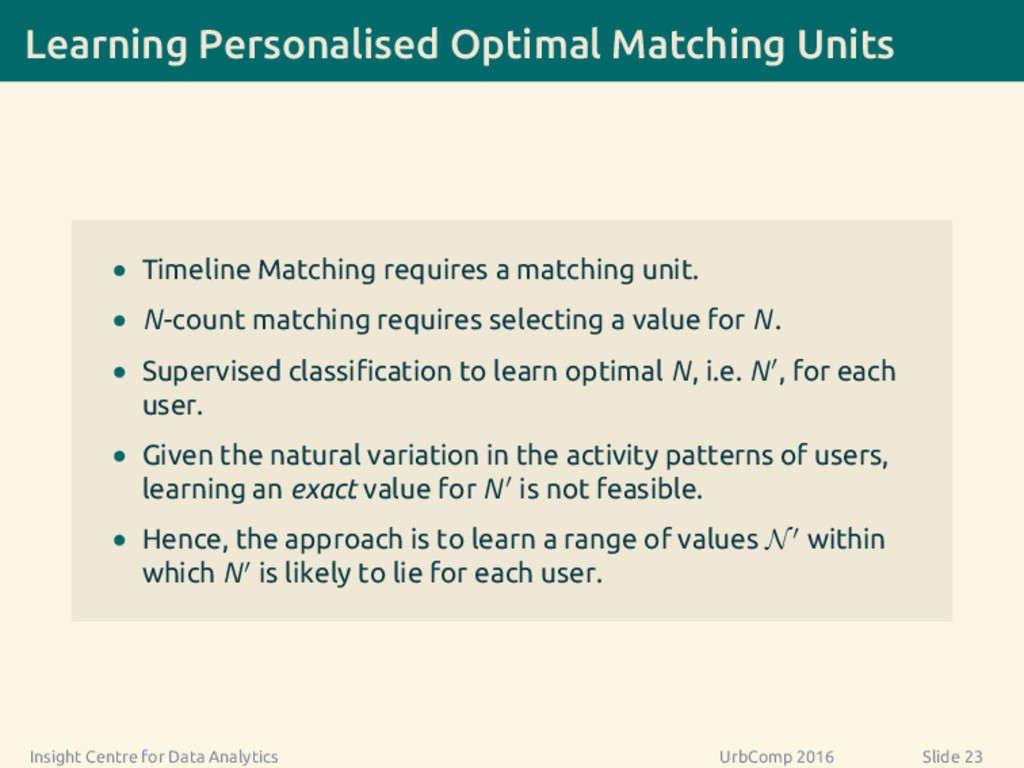
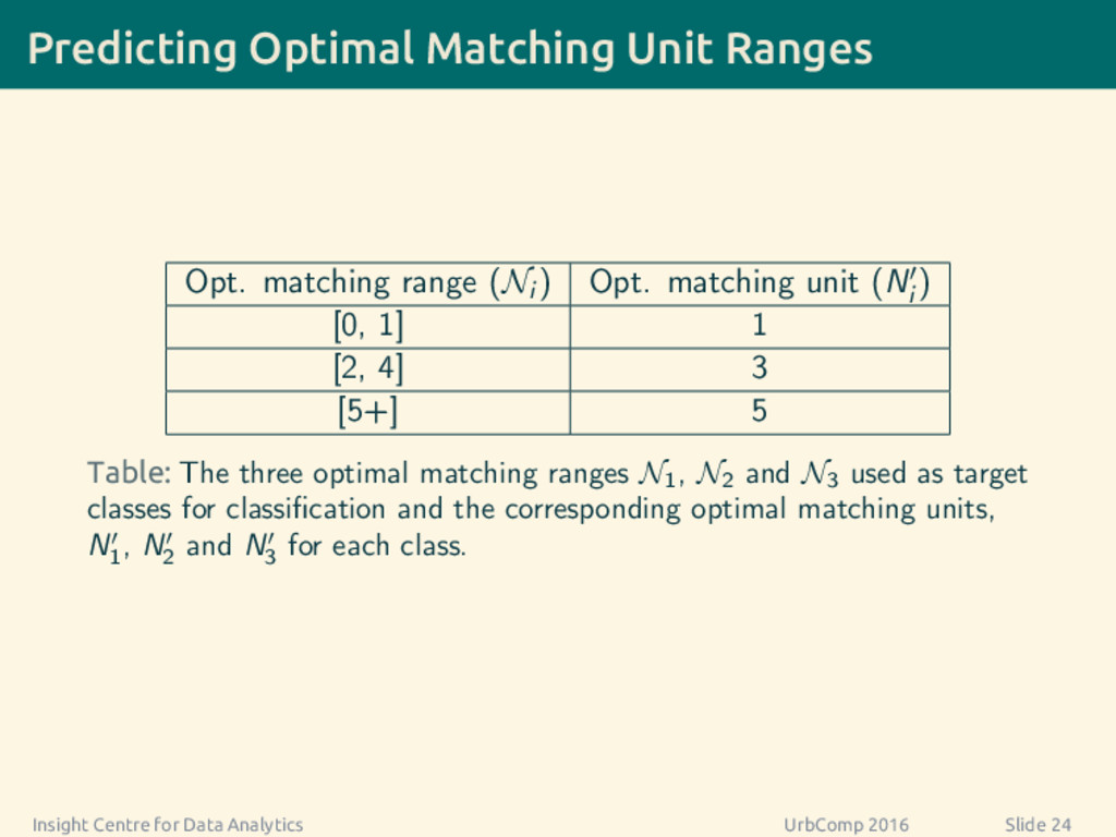
  33. Learning Personalised Optimal Matching Units • Timeline Matching requires a

    matching unit. • N-count matching requires selecting a value for N. • Supervised classification to learn optimal N, i.e. N , for each user. • Given the natural variation in the activity patterns of users, learning an exact value for N is not feasible. • Hence, the approach is to learn a range of values N within which N is likely to lie for each user. Insight Centre for Data Analytics UrbComp 2016 Slide 23
  34. Predicting Optimal Matching Unit Ranges Opt. matching range (Ni )

    Opt. matching unit (Ni ) [0, 1] 1 [2, 4] 3 [5+] 5 Table: The three optimal matching ranges N1 , N2 and N3 used as target classes for classification and the corresponding optimal matching units, N1 , N2 and N3 for each class. Insight Centre for Data Analytics UrbComp 2016 Slide 24
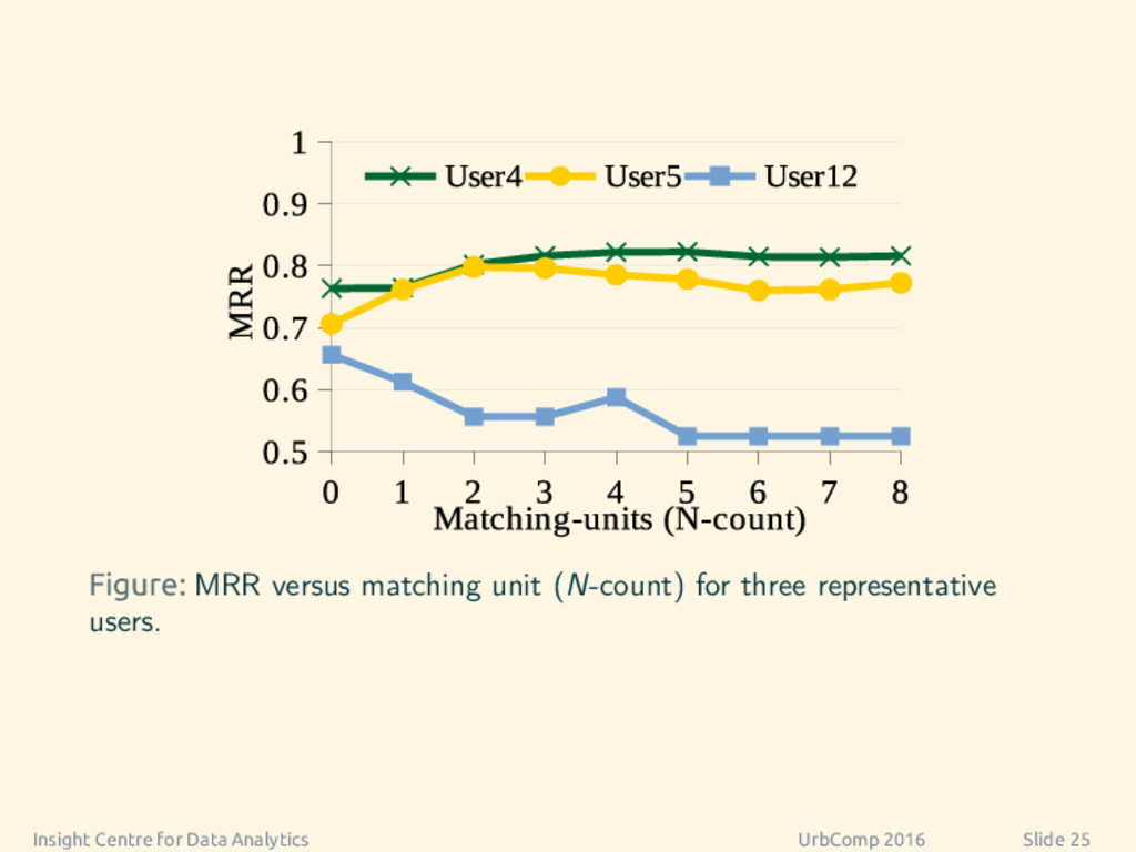
  35. Figure: MRR versus matching unit (N-count) for three representative users.

    Insight Centre for Data Analytics UrbComp 2016 Slide 25
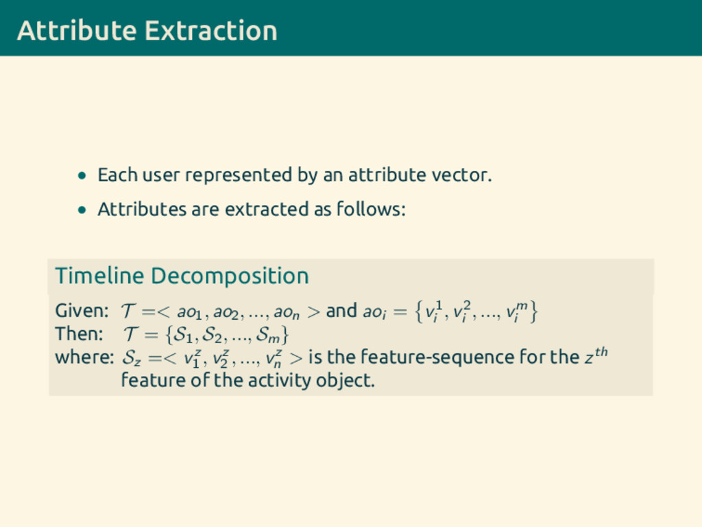
  36. Attribute Extraction • Each user represented by an attribute vector.

    • Attributes are extracted as follows: Timeline Decomposition Given: T =< ao1, ao2, ..., aon > and aoi = v1 i , v2 i , ..., vm i Then: T = {S1, S2, ..., Sm} where: Sz =< vz 1 , vz 2 , ..., vz n > is the feature-sequence for the zth feature of the activity object.
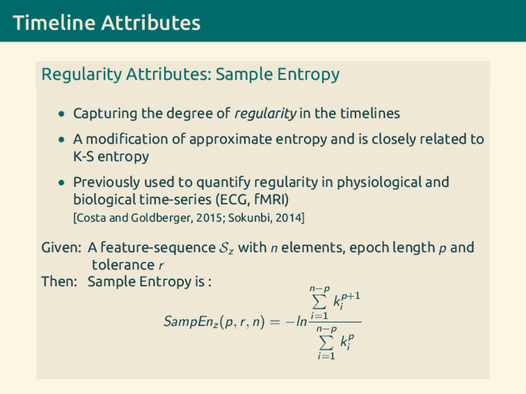
  37. Timeline Attributes Regularity Attributes: Sample Entropy • Capturing the degree

    of regularity in the timelines • A modification of approximate entropy and is closely related to K-S entropy • Previously used to quantify regularity in physiological and biological time-series (ECG, fMRI) [Costa and Goldberger, 2015; Sokunbi, 2014]
  38. Timeline Attributes Regularity Attributes: Sample Entropy • Capturing the degree

    of regularity in the timelines • A modification of approximate entropy and is closely related to K-S entropy • Previously used to quantify regularity in physiological and biological time-series (ECG, fMRI) [Costa and Goldberger, 2015; Sokunbi, 2014] Given: A feature-sequence Sz with n elements, epoch length p and tolerance r Then: Sample Entropy is : SampEnz (p, r, n) = −ln n−p i=1 kp+1 i n−p i=1 kp i
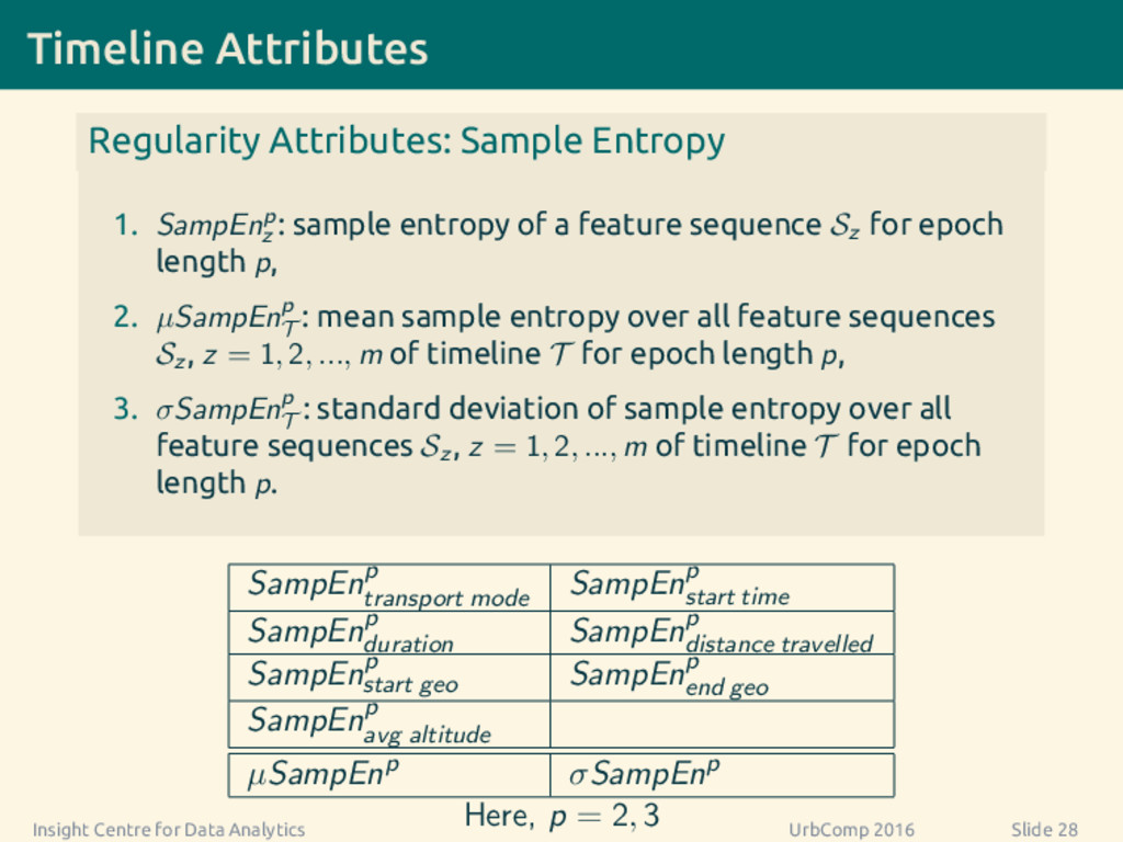
  39. Timeline Attributes Regularity Attributes: Sample Entropy 1. SampEnp z :

    sample entropy of a feature sequence Sz for epoch length p, 2. µSampEnp T : mean sample entropy over all feature sequences Sz , z = 1, 2, ..., m of timeline T for epoch length p, 3. σSampEnp T : standard deviation of sample entropy over all feature sequences Sz , z = 1, 2, ..., m of timeline T for epoch length p. SampEnp transport mode SampEnp start time SampEnp duration SampEnp distance travelled SampEnp start geo SampEnp end geo SampEnp avg altitude µSampEnp σSampEnp Here, p = 2, 3 Insight Centre for Data Analytics UrbComp 2016 Slide 28
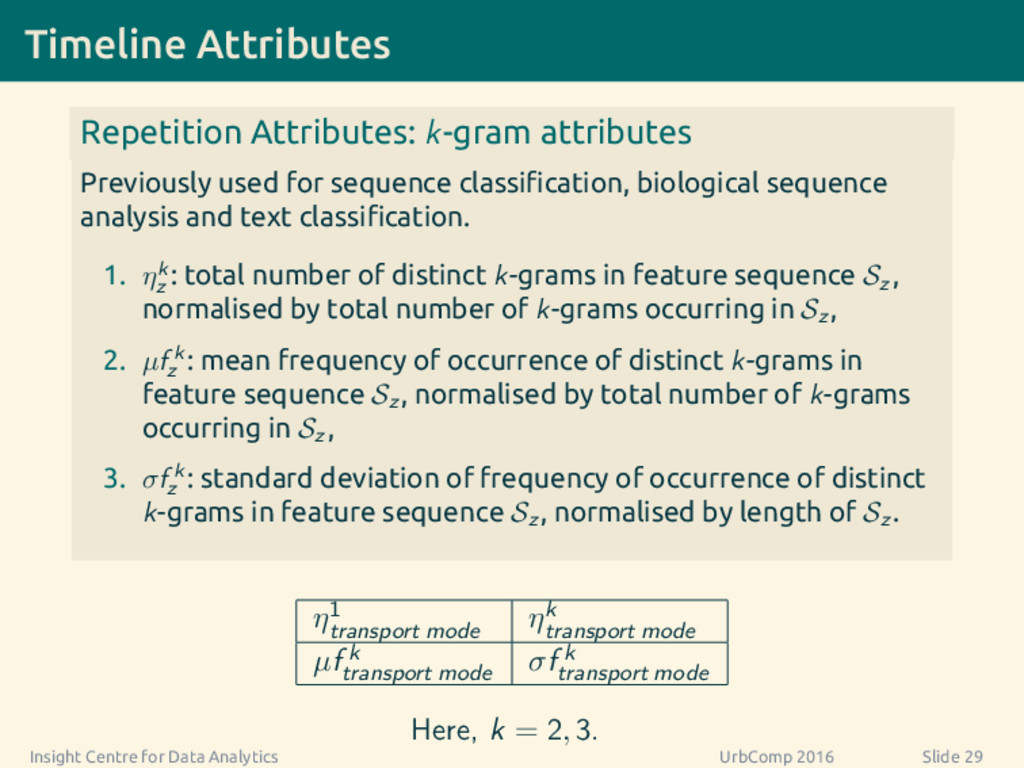
  40. Timeline Attributes Repetition Attributes: k-gram attributes Previously used for sequence

    classification, biological sequence analysis and text classification. 1. ηk z : total number of distinct k-grams in feature sequence Sz , normalised by total number of k-grams occurring in Sz , 2. µf k z : mean frequency of occurrence of distinct k-grams in feature sequence Sz , normalised by total number of k-grams occurring in Sz , 3. σf k z : standard deviation of frequency of occurrence of distinct k-grams in feature sequence Sz , normalised by length of Sz . η1 transport mode ηk transport mode µf k transport mode σf k transport mode Here, k = 2, 3. Insight Centre for Data Analytics UrbComp 2016 Slide 29
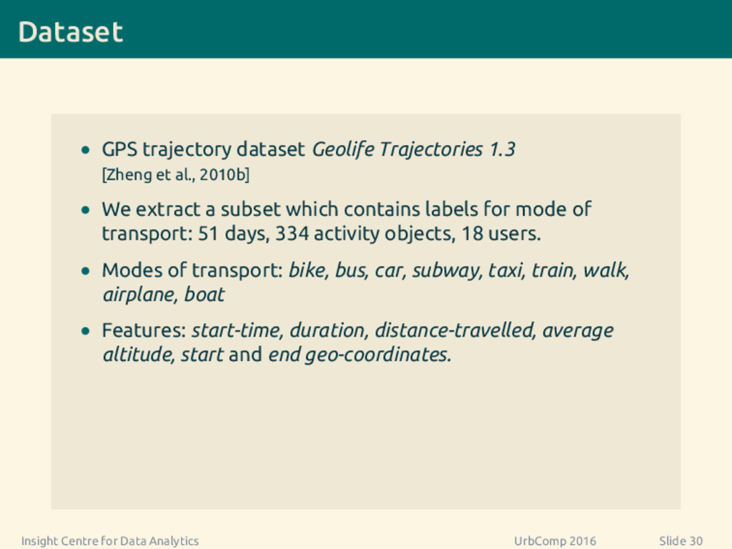
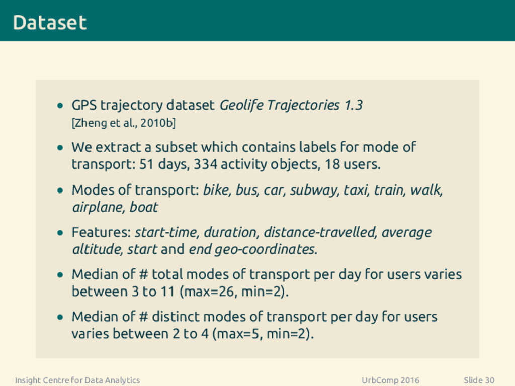
  41. Dataset • GPS trajectory dataset Geolife Trajectories 1.3 [Zheng et

    al., 2010b] • We extract a subset which contains labels for mode of transport: 51 days, 334 activity objects, 18 users. • Modes of transport: bike, bus, car, subway, taxi, train, walk, airplane, boat • Features: start-time, duration, distance-travelled, average altitude, start and end geo-coordinates. Insight Centre for Data Analytics UrbComp 2016 Slide 30
  42. Dataset • GPS trajectory dataset Geolife Trajectories 1.3 [Zheng et

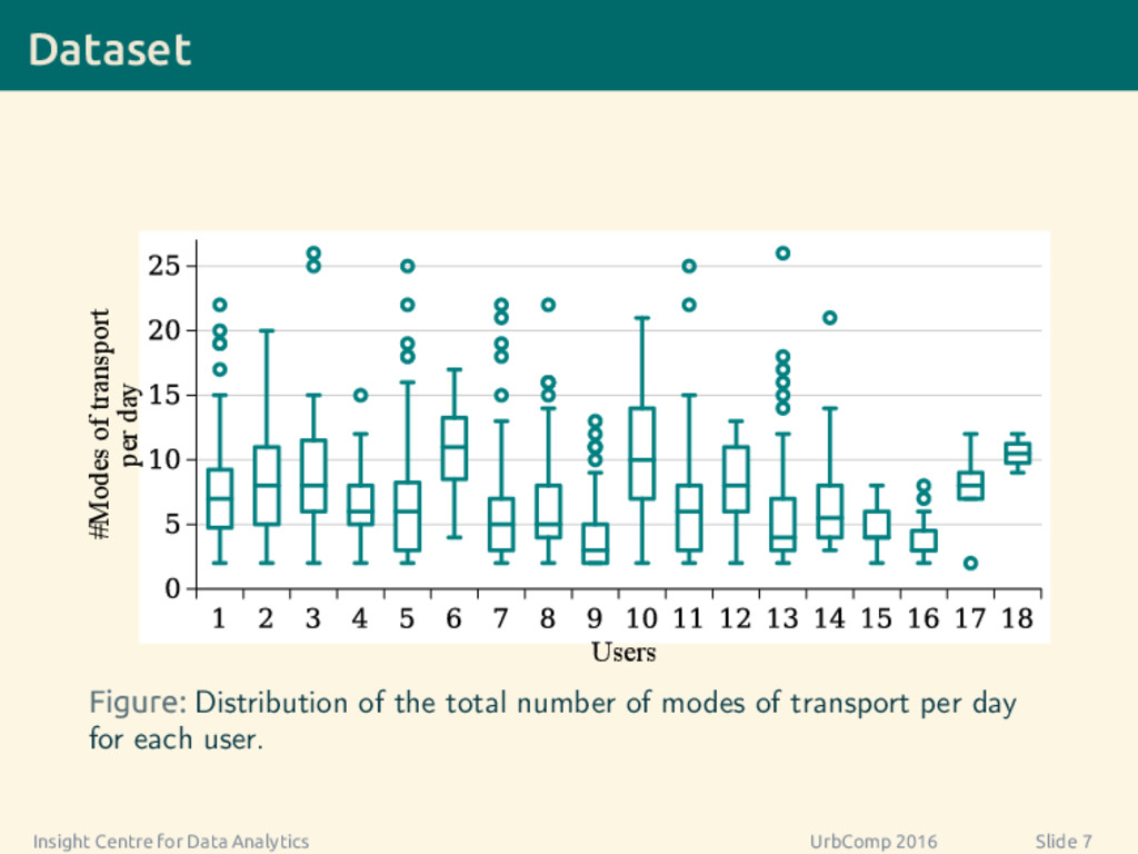
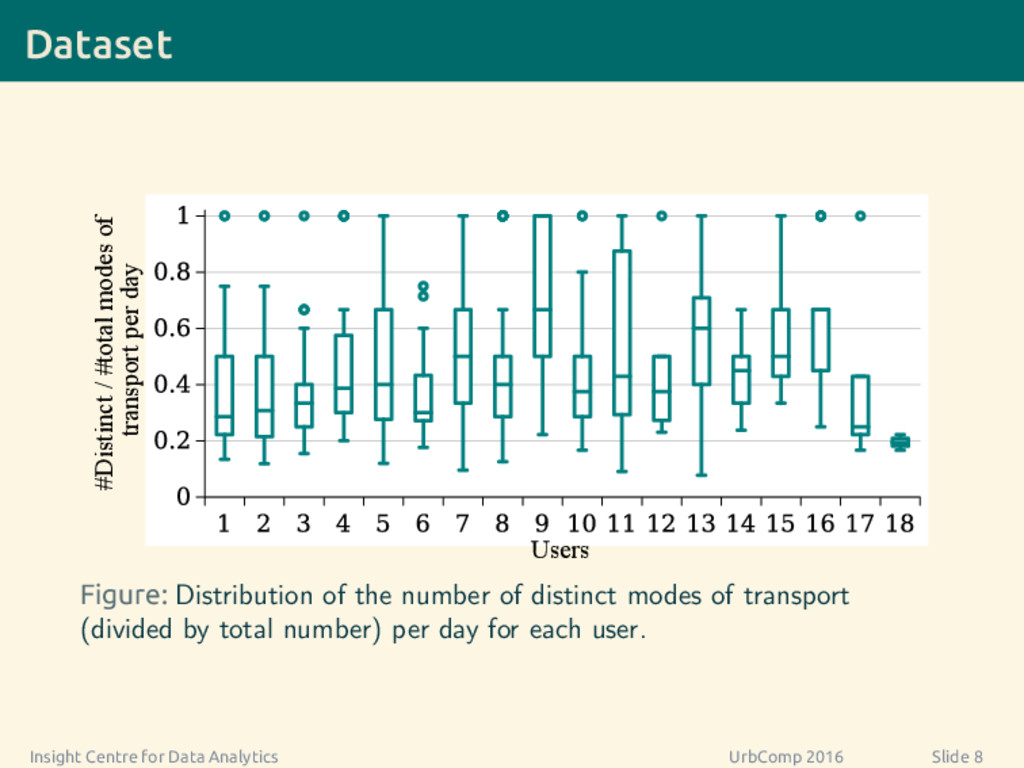
    al., 2010b] • We extract a subset which contains labels for mode of transport: 51 days, 334 activity objects, 18 users. • Modes of transport: bike, bus, car, subway, taxi, train, walk, airplane, boat • Features: start-time, duration, distance-travelled, average altitude, start and end geo-coordinates. • Median of # total modes of transport per day for users varies between 3 to 11 (max=26, min=2). • Median of # distinct modes of transport per day for users varies between 2 to 4 (max=5, min=2). Insight Centre for Data Analytics UrbComp 2016 Slide 30
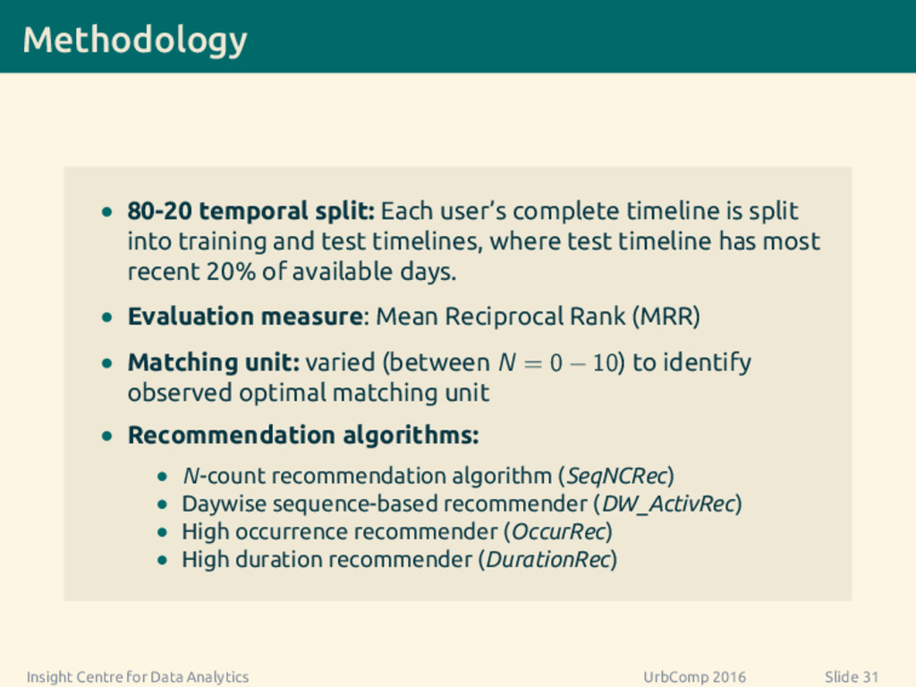
  43. Methodology • 80-20 temporal split: Each user’s complete timeline is

    split into training and test timelines, where test timeline has most recent 20% of available days. • Evaluation measure: Mean Reciprocal Rank (MRR) • Matching unit: varied (between N = 0 − 10) to identify observed optimal matching unit • Recommendation algorithms: • N-count recommendation algorithm (SeqNCRec) • Daywise sequence-based recommender (DW_ActivRec) • High occurrence recommender (OccurRec) • High duration recommender (DurationRec) Insight Centre for Data Analytics UrbComp 2016 Slide 31
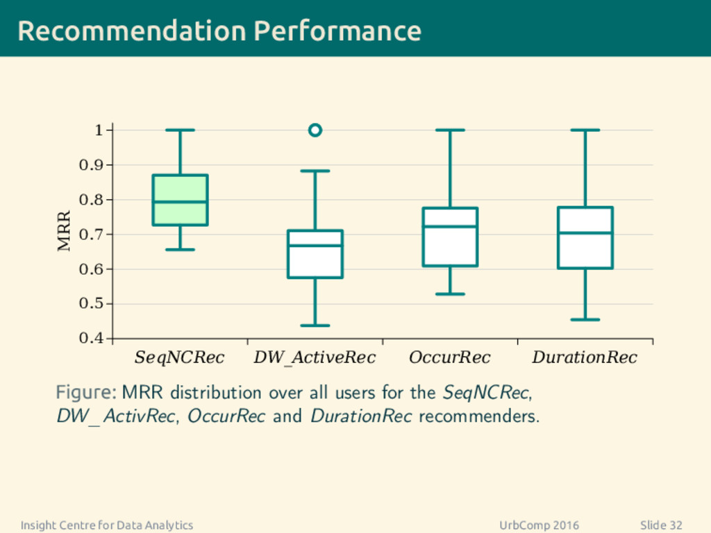
  44. Recommendation Performance SeqNCRec DW_ActiveRec OccurRec DurationRec 0.4 0.5 0.6 0.7

    0.8 0.9 1 MRR Figure: MRR distribution over all users for the SeqNCRec, DW_ActivRec, OccurRec and DurationRec recommenders. Insight Centre for Data Analytics UrbComp 2016 Slide 32
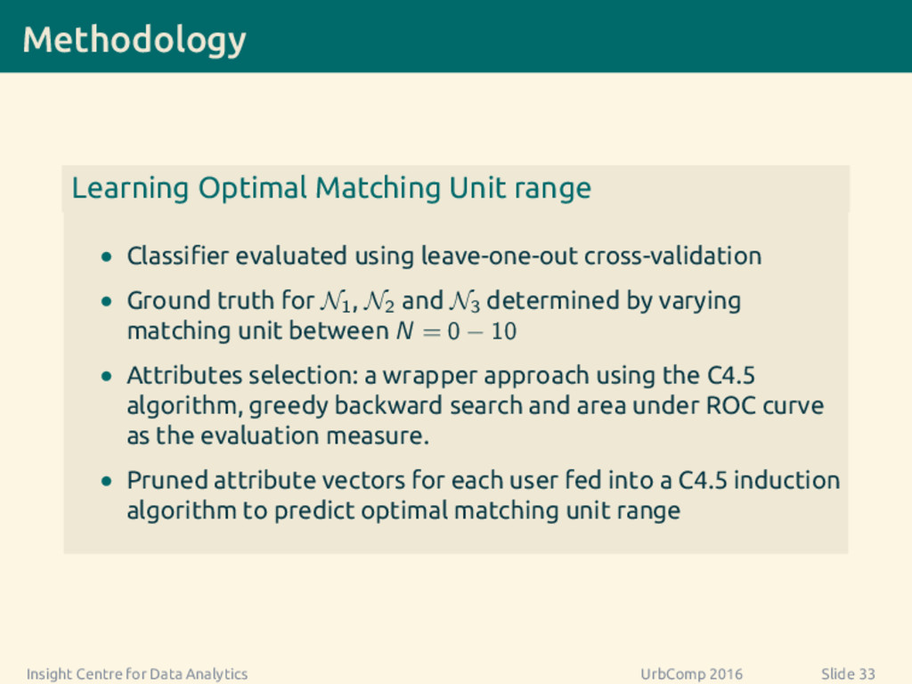
  45. Methodology Learning Optimal Matching Unit range • Classifier evaluated using

    leave-one-out cross-validation • Ground truth for N1 , N2 and N3 determined by varying matching unit between N = 0 − 10 • Attributes selection: a wrapper approach using the C4.5 algorithm, greedy backward search and area under ROC curve as the evaluation measure. • Pruned attribute vectors for each user fed into a C4.5 induction algorithm to predict optimal matching unit range Insight Centre for Data Analytics UrbComp 2016 Slide 33
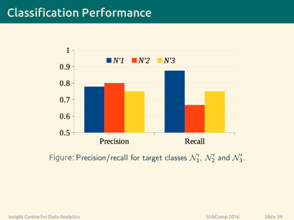
  46. Classification Performance Figure: Precision/recall for target classes N1 , N2

    and N3 . Insight Centre for Data Analytics UrbComp 2016 Slide 34
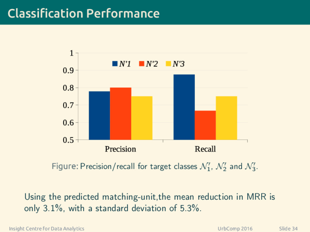
  47. Classification Performance Figure: Precision/recall for target classes N1 , N2

    and N3 . Using the predicted matching-unit,the mean reduction in MRR is only 3.1%, with a standard deviation of 5.3%. Insight Centre for Data Analytics UrbComp 2016 Slide 34
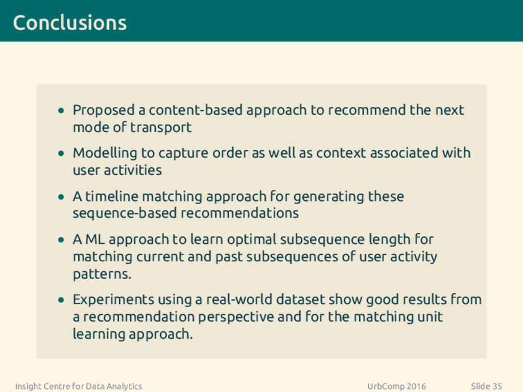
  48. Conclusions • Proposed a content-based approach to recommend the next

    mode of transport • Modelling to capture order as well as context associated with user activities • A timeline matching approach for generating these sequence-based recommendations • A ML approach to learn optimal subsequence length for matching current and past subsequences of user activity patterns. • Experiments using a real-world dataset show good results from a recommendation perspective and for the matching unit learning approach. Insight Centre for Data Analytics UrbComp 2016 Slide 35
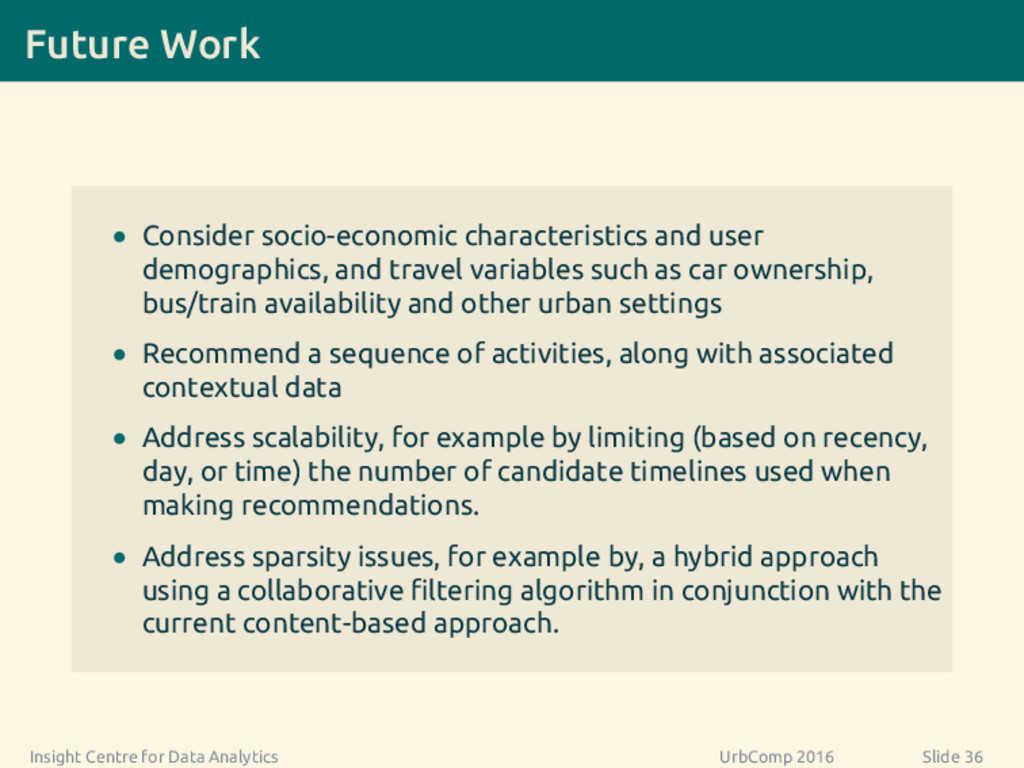
  49. Future Work • Consider socio-economic characteristics and user demographics, and

    travel variables such as car ownership, bus/train availability and other urban settings • Recommend a sequence of activities, along with associated contextual data • Address scalability, for example by limiting (based on recency, day, or time) the number of candidate timelines used when making recommendations. • Address sparsity issues, for example by, a hybrid approach using a collaborative filtering algorithm in conjunction with the current content-based approach. Insight Centre for Data Analytics UrbComp 2016 Slide 36
  50. References I G. Adomavicius and A. Tuzhilin. Toward the next

    generation of recommender systems: A survey of the state-of-the-art and possible extensions. IEEE Trans. on Knowl. and Data Eng., 17(6):734–749, June 2005. G. Adomavicius, B. Mobasher, F. Ricci, and A. Tuzhilin. Context-aware recommender systems. AI Magazine, 32(3), 2011. T. Bohnenberger and A. Jameson. When policies are better than plans: Decision-theoretic planning of recommendation sequences. In Proceedings of the 6th International Conference on Intelligent User Interfaces, IUI ’01, pages 21–24. ACM, 2001. M. D. Costa and A. L. Goldberger. Generalized multiscale entropy analysis: Application to quantifying the complex volatility of human heartbeat time series. Entropy, 17(3):1197–1203, 2015. M. Deshpande and G. Karypis. Selective Markov models for predicting web page accesses. ACM Trans. Internet Technol., 4(2):163–184, May 2004. B. Hayes. Crinkly curves. American Scientist, 101(3):178, 2013. G. Kumar, H. Jerbi, C. Gurrin, and M. P. O’Mahony. Towards activity recommendation from lifelogs. In Proceedings of the 16th International Conference on Information Integration and Web-based Applications & Services, iiWAS ’14, pages 87–96. ACM, 2014. Q. Li, Y. Zheng, X. Xie, Y. Chen, W. Liu, and W.-Y. Ma. Mining user similarity based on location history. In Proceedings of the 16th ACM SIGSPATIAL International Conference on Advances in Geographic Information Systems, GIS ’08, pages 34:1–34:10. ACM, 2008.
  51. References II H. Sagan. Space-filling curves. Springer Science & Business

    Media, 2012. G. Shani, D. Heckerman, and R. I. Brafman. An MDP-based recommender system. J. Mach. Learn. Res., 6:1265–1295, Dec. 2005. M. O. Sokunbi. Sample entropy reveals high discriminative power between young and elderly adults in short fMRI data sets. Frontiers in neuroinformatics, 8, 2014. Y. Sun, N. J. Yuan, X. Xie, K. McDonald, and R. Zhang. Collaborative nowcasting for contextual recommendation. In Proceedings of the 25th International Conference on World Wide Web, WWW ’16, pages 1407–1418. International World Wide Web Conferences Steering Committee, 2016. P. Symeonidis, A. Papadimitriou, Y. Manolopoulos, P. Senkul, and I. Toroslu. Geo-social recommendations based on incremental tensor reduction and local path traversal. In Proceedings of the 3rd ACM SIGSPATIAL International Workshop on Location-Based Social Networks, LBSN ’11, pages 89–96. ACM, 2011. C.-Y. Wang, Y.-H. Wu, and S.-C. T. Chou. Toward a ubiquitous personalized daily-life activity recommendation service with contextual information: A services science perspective. Information Systems and E-Business Management, 8(1):13–32, January 2010. H. Yoon, Y. Zheng, X. Xie, and W. Woo. Smart itinerary recommendation based on user-generated GPS trajectories. In Proceedings of the 7th International Conference on Ubiquitous Intelligence and Computing, UIC’10, pages 19–34. Springer-Verlag, 2010.
  52. References III V. W. Zheng, B. Cao, Y. Zheng, X.

    Xie, and Q. Yang. Collaborative filtering meets mobile recommendation: A user-centered approach. In AAAI 2010. Association for Computing Machinery, Inc., July 2010a. V. W. Zheng, Y. Zheng, X. Xie, and Q. Yang. Towards mobile intelligence: Learning from GPS history data for collaborative recommendation. Artif. Intell., 184-185: 17–37, June 2012. Y. Zheng, L. Zhang, X. Xie, and W.-Y. Ma. Mining interesting locations and travel sequences from GPS trajectories. In Proceedings of the 18th International Conference on World Wide Web, WWW ’09, pages 791–800. ACM, 2009. Y. Zheng, X. Xie, and W.-Y. Ma. Geolife: A collaborative social networking service among user, location and trajectory. IEEE Database Engineering Bulletin, June 2010b.
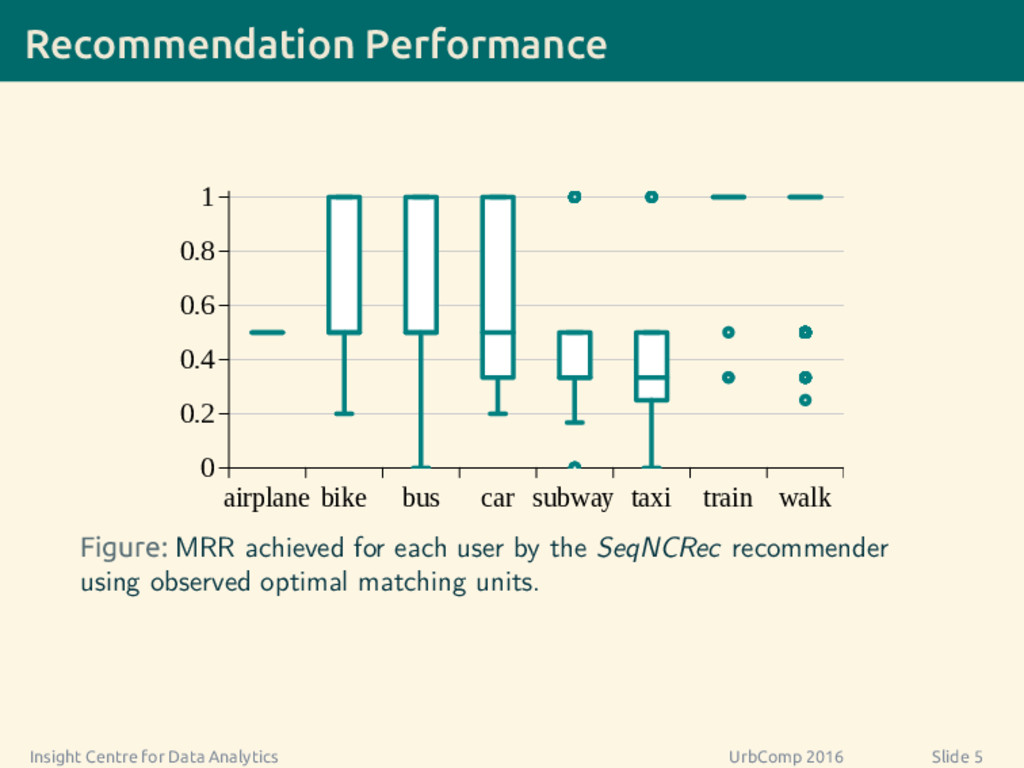
  53. Recommendation Performance airplane bike bus car subway taxi train walk

    0 0.2 0.4 0.6 0.8 1 Figure: MRR achieved for each user by the SeqNCRec recommender using observed optimal matching units. Insight Centre for Data Analytics UrbComp 2016 Slide 5
  54. Two-level Distance • Inspired by edit distance • Adapted for

    sequence of objects 09:00 10:05 10:35 10:50 11:32 11:25
  55. Two-level Distance • Inspired by edit distance • Adapted for

    sequence of objects 09:00 10:05 10:35 10:50 11:32 Step 1 Align activities 11:25 ( ( dactivity (T1, T2) = r i=1 wobj × cins + s j=1 wobj × cdel + t k=1 wobj × csub
  56. Two-level Distance • Inspired by edit distance • Adapted for

    sequence of objects 09:00 10:05 10:35 10:50 11:32 Step 1 Step 2 Align activities Align features 11:25 ( ( ( ( d(T1, T2) = dactivity (T1, T2) + n i=1 dfeature(ao1 i , ao2 i ) .
  57. Dataset Users #Modes of transport per day Figure: Distribution of
    the total number of modes of transport per day for each user. Insight Centre for Data Analytics UrbComp 2016 Slide 7
  58. Dataset Users #Distinct / #total modes of transport per day
    Figure: Distribution of the number of distinct modes of transport (divided by total number) per day for each user. Insight Centre for Data Analytics UrbComp 2016 Slide 8
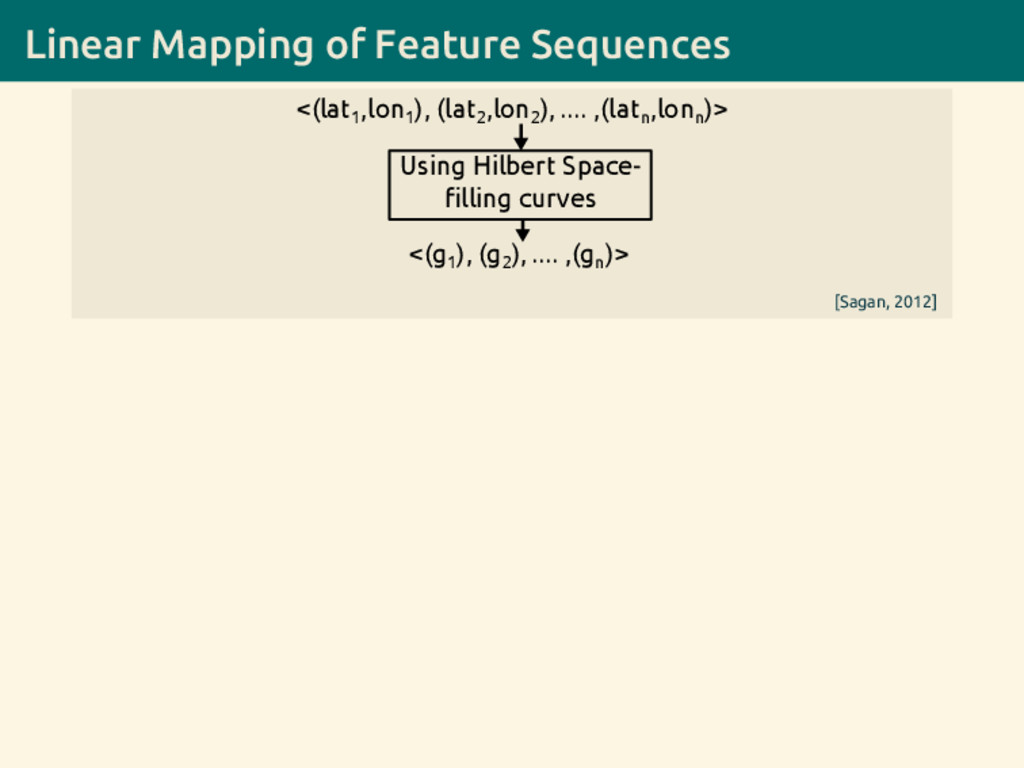
  59. Linear Mapping of Feature Sequences Using Hilbert Space- filling curves

    <(lat 1 ,lon 1 ), (lat 2 ,lon 2 ), .... ,(lat n ,lon n )> <(g 1 ), (g 2 ), .... ,(g n )> [Sagan, 2012]
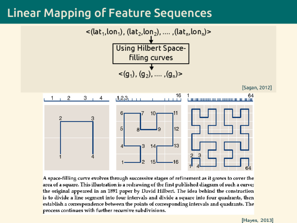
  60. Linear Mapping of Feature Sequences Using Hilbert Space- filling curves

    <(lat 1 ,lon 1 ), (lat 2 ,lon 2 ), .... ,(lat n ,lon n )> <(g 1 ), (g 2 ), .... ,(g n )> [Sagan, 2012] [Hayes, 2013]
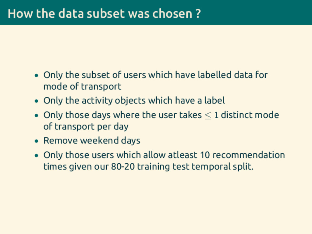
  61. How the data subset was chosen ? • Only the

    subset of users which have labelled data for mode of transport • Only the activity objects which have a label • Only those days where the user takes ≤ 1 distinct mode of transport per day • Remove weekend days • Only those users which allow atleast 10 recommendation times given our 80-20 training test temporal split.
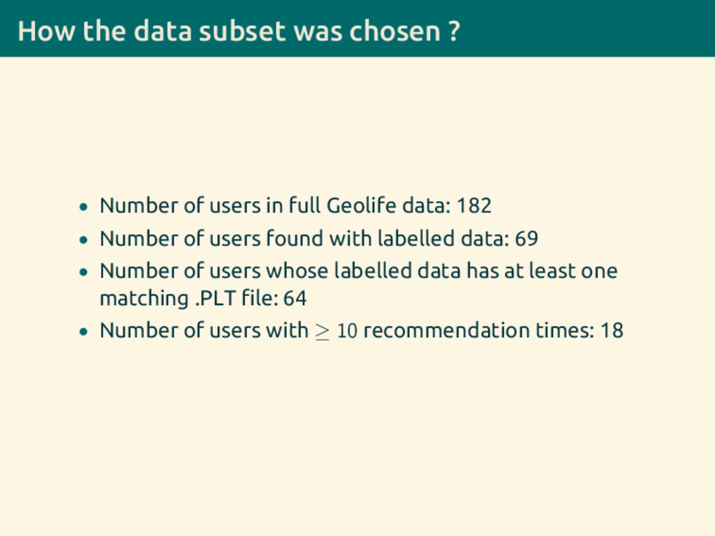
  62. How the data subset was chosen ? • Number of

    users in full Geolife data: 182 • Number of users found with labelled data: 69 • Number of users whose labelled data has at least one matching .PLT file: 64 • Number of users with ≥ 10 recommendation times: 18