Natural Language Visualization with Scattertext

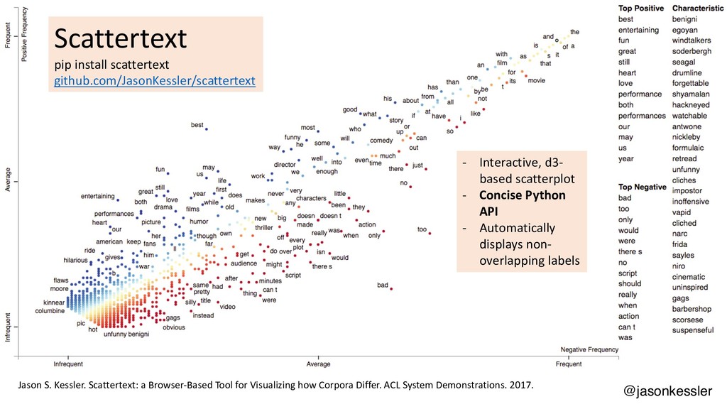
Scattertext is a Python package that lets you compare and contrast how words and phrases are used differently in two types of documents, producing interactive, Javascript-based visualizations. This talk will cover the use of Scattertext, issues in creating dense scatterplots, and discuss statistical term-association and phrase identification algorithms. The code used in the talk will be available as a repository on my Github account, http://www.github.com/JasonKessler/GlobalAI2018

Transcript

1. Natural Language Visualization with Scattertext Jason S. Kessler* Global AI Conference April 27, 2018 Code for all visualizations is available at: https://github.com/JasonKessler/GlobalAI2018 $ pip3 install scattertext @jasonkessler *No, not that Jason Kessler
2. Lexicon speculation Bo Pang, Lillian Lee and Shivakumar Vaithyanathan. Thumbs up? Sentiment classification using machine learning techniques. EMNLP. 2002. (ACL 2018 Test of Time Award Winner) @jasonkessler
3. Bo Pang, Lillian Lee and Shivakumar Vaithyanathan. Thumbs up? Sentiment classification using machine learning techniques. EMNLP. 2002. Lexicon mining ≈ lexicon speculation @jasonkessler
4. Language and Demographics Christian Rudder: http://blog.okcupid.com/index.php/page/7/ hobos almond butter 100 Years of Solitude Bikram yoga @jasonkessler
5. Source: http://blog.okcupid.com/index.php/page/7/ (Rudder 2010) OKCupid: Words and phrases that distinguish white men. @jasonkessler
6. Explanation OKCupid: Words and phrases that distinguish Latin men. Source: http://blog.okcupid.com/index.php/page/7/ (Rudder 2010) @jasonkessler
7. Ranking with everyone else The smaller the distance from the top left, the higher the association with white men Source: Christian Rudder. Dataclysm. 2014. Phish is highly associated with white men Kpop is not @jasonkessler
8. @jasonkessler my blue eyes Source: Christian Rudder. Dataclysm. 2014.
9. Scattertext pip install scattertext github.com/JasonKessler/scattertext @jasonkessler Jason S. Kessler. Scattertext: a Browser-Based Tool for Visualizing how Corpora Differ. ACL System Demonstrations. 2017. - Interactive, d3- based scatterplot - Concise Python API - Automatically displays non- overlapping labels
10. Scaled F-Score • Term-class* associations: • “Good” is associated with the “positive” class • “Bad” with the class “negative” • Core intuition: association relies on two necessary factors • Frequency: How often a term occurs in a class • Precision: P(class|document contains term) • F-Score: • Information retrieval evaluation metric • Harmonic mean between precision and recall • Requires both metrics to be high • *Term: is defined to be a word, phrase or other discrete linguistic element @jasonkessler
11. @jasonkessler Precision Frequency Naïve approach
12. @jasonkessler Precision Frequency Naïve approach Y-axis: - Precision, i.e. P(class|term), roughly normal distribution - Mean ≅ 0.5, sd ≅ 0.4, X-axis: - Frequency, i.e. P(term|class), roughly power distribution - Mean ≅ 0.00008, sd ≅ 0.008 Color: - Harmonic mean of precision and frequency (blue=high, red=low)
13. @jasonkessler Precision Frequency Problem: • Top words are just stop words. • Why? • Harmonic mean of uneven distributions. • Most words have prec of ~0.5, leads harmonic mean to rely on frequency.
14. Fix: Normalize Precision and Frequency • Task: make precision and frequency similarly distributed • How: take normal CDF of each term’s precision and frequency • Mean and std. computed from data • Right: log normal CDF @jasonkessler This area is the log-normal CDF of the term “beauty” (0.938 ∈ [0,1]). Each tick mark is the log- frequency of a term. *log-normal CDF isn’t used in these charts
15. Scaled-F-Score @jasonkessler NormCDF - Precision NormCDF - Frequency
16. Positive Scaled-F-Score Good: positive terms make sense! Still some function words, but that’s okay. Note These frequent terms are all very close to 1 on the x-axis, but are ordered NormCDF - Precision NormCDF - Frequency @jasonkessler
17. Pos Freq. Neg Freq. Prec. Freq % Raw Hmean Prec. CDF Freq. CDF Scaled F-Score best 108 36 75.00% 0.22% 0.44% 71.95% 99.50% 83.51% entertaining 58 13 81.69% 0.12% 0.24% 77.07% 90.94% 83.43% fun 73 26 73.74% 0.15% 0.30% 70.92% 95.63% 81.44% heart 45 11 80.36% 0.09% 0.18% 76.09% 84.49% 80.07% Top Scaled-F Score Terms Note: normalized precision and frequency are on comparable scales, allowing for the harmonic mean to take both into account.
18. Problem: highly negative terms are all low frequency NormCDF - Precision NormCDF - Frequency @jasonkessler Solution: • Compute Scaled F- Score association scores for negative reviews. • Use the highest score
19. Scaled-F-Score Positive Scaled F-Score @jasonkessler Negative Scaled F- Score Note: only one obviously negative term
20. @jasonkessler Scaled-F-Score by log- frequency The score can be overly sensitive to very frequent terms, but still doesn’t score them very highly Scaled F- Score Log Frequency
21. Why not use TF-IDF? • Drastically favors low frequency terms • term in all classes -> idf=1 -> score=0 TF-IDF(Positive) - TF-IDF(Negative) Log Frequency TF IDF
22. Burt Monroe, Michael Colaresi and Kevin Quinn. Fightin' words: Lexical feature selection and evaluation for identifying the content of political conflict. Political Analysis. 2008. @jasonkessler Monroe et. al (2009) approach • Bayesian approach to term- association • Likelihood: Z-score of log-odds- ratio • Prior: Term frequency in a background corpus • Posterior: Z-score of log-odds-ratio with background counts as smoothing values Popular, but much more tweaking to get to work than Scaled F Score.
23. @jasonkessler Scattertext reimplementation of Monroe et al. See http://nbviewer.jupyter.org/github/JasonKessler/PuPPyTalk/blob/master/notebooks/Class-Association-Scores.ipynb for code. Scattertext implementation (with prior weighting modifications)
24. In defense of stop words Cindy K. Chung and James W. Pennebaker. Counting Little Words in Big Data: The Psychology of Communities, Culture, and History. EASP. 2012 In times of shared crisis, “we” use increases, while “I” use decreases. I/we: age, social integration I: lying, social rank @jasonkessler
25. Function words and gender Newman, ML; Groom, CJ; Handelman LD, Pennebaker, JW. Gender Differences in Language Use: An Analysis of 14,000 Text Samples. 2008. LIWC Dimension Bold: entirely stop words Effect Size (Cohen’s d) (>0 F, <0 M) MANOVA p<.001 All Pronouns (esp. 3rd person) 0.36 Present tense verbs (walk, is, be) 0.18 Feeling (touch, hold, feel) 0.17 Certainty (always, never) 0.14 Word count NS Numbers -0.15 Prepositions -0.17 Words >6 letters -0.24 Swear words -0.22 Articles -0.24 • Performed on a variety of language categories, including speech. • Other studies have found that function words are the best predictors of gender. @jasonkessler
26. Function word usage is counter-intuitive - James W. Pennebaker, Carla J. Groom, Daniel Loew, James M. Dabbs. Testosterone as a Social Inhibitor: Two Case Studies of the Effect of Testosterone Treatment on Language. 2004. - Susan C. Herring, Anna Martinson. Assessing Gender Authenticity in Computer-Mediated Language Use: Evidence From an Identity Game. Journal of Language and Social Psychology. 2004. • Pennebaker et al: • Testosterone levels (in two therapeutic settings) predict: • Modest but significant decreases in: • Pronouns referring to others (ex: we, she, they) • Communication verbs (ex: hear, say) • Modest but significant decreases in: • Optimism words (ex: energy, upbeat) • Negative (but statistically insignificant) correlation with subject’s beliefs about testosterone and category usage! • Does not entirely explain gender differences. • Herring et al: • Subjects tasked with impersonating opposite gender in online game • Discussed stereotypical topics (cars, shopping) but didn’t change stylistic cues @jasonkessler
27. Clickbait: what works? @jasonkessler
28. Clickbait corpus • Facebook posts from BuzzFeed, NY Times, etc/ from 2010s. • Includes headline and the number of Facebook likes • Scraped by researcher Max Woolf at github.com/minimaxir/clickbait-cluster. • We’ll separate articles from 2016 into the upper third and lower third of likes. • Identify words and phrases that predict likes. • Begin with noun phrases identified from Phrase Machine (Handler et al. 2016) • Filter out redundant NPs. Abram Handler, Matt Denny, Hanna Wallach, and Brendan O'Connor. Bag of what? Simple noun phrase extraction for corpus analysis. NLP+CSS Workshop at EMNLP 2016. @jasonkessler
29. @jasonkessler Scaled-F-Score of engagement by noun phrase
30. @jasonkessler Scaled-F-Score of engagement by unigram Messier, but psycholinguist information: 3rd person pronouns -> high engagement; 2nd person low “dies”: obit Can, guess, how: questions.
31. Clickbait corpus • How do terms with similar meanings differ in terms of their engagement rates? • Use Gensim (https://radimrehurek.com/gensim/) to find word embeddings • Use UMAP (McInnes and Healy 2018) to project them into two dimensions, and explore them with Scattertext. • Locally groups words with similar embeddings together. • Better alternative to T-SNE; allows for cosine instead of Euclidean distance criteria Leland McInnes, John Healy. UMAP: Uniform Manifold Approximation and Projection for Dimension Reduction. Arxiv. 2018. @jasonkessler
32. @jasonkessler This island is mostly food related. “Chocolate” and “cake” are highly engaging, but “breakfast” has predictive of low engagement. Term positions from determined by UMAP, color by Scaled F-Score for engagement.
33. Clickbait corpus • How do the Times and Buzzfeed differ in what they talk about, and their content engages their readers? • Scattertext can easily create visualizations to help answer these questions. • First, we’ll look at how what engages for Buzzfeed contrasts with what engages for the Times, and vice versa Leland McInnes, John Healy. UMAP: Uniform Manifold Approximation and Projection for Dimension Reduction. Arxiv. 2018. @jasonkessler
34. Oddly, NY Times readers distinctly like articles about sex, death, and which are written in a smug tone. This chart doesn’t give a good sense of what language is more associated with one site. @jasonkessler
35. This chart let’s you know how Buzzfeed and the Times are distinct, while still distinguishing engaging content, @jasonkessler
36. Thank you! Questions? @jasonkessler Jason S. Kessler Global AI Conference April 27, 2018 https://github.com/JasonKessler/GlobalAI2018