Upgrade to Pro — share decks privately, control downloads, hide ads and more …

Primitive Recursive Bars Are Inductive

Avatar for Jonathan Sterling Jonathan Sterling
August 17, 2016
170

Primitive Recursive Bars Are Inductive

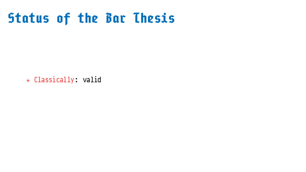
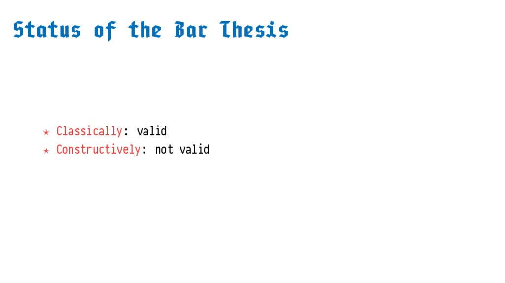
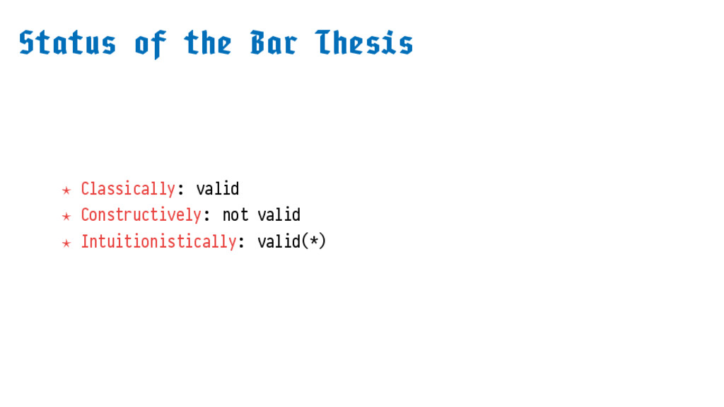
The Church-Turing Thesis is a scientific hypothesis as to the nature of effective computation at lower type; the nature of higher type computability, however, is far from settled and admits many possible models. In the 1920s, L.E.J. Brouwer (the father of Intuitionism) gave a mysterious "proof" of an induction principle for infinite trees called the Bar Theorem, which has many consequences, including a constructive contrapositive to König's Lemma (the Fan Theorem).
We situate the Bar Theorem more generally as "Brouwer's Thesis", a scientific claim about the nature of higher-type computability which may be contrasted with competing explanations, including recursive realizability and Turing machines. Then, we demonstrate using a technique called Effectful Forcing that Brouwer's Bar Theorem is constructively valid for any bar which can be written in Gödel's System T of primitive recursive arithmetic of finite type, a very simple programming language.

Avatar for Jonathan Sterling

Jonathan Sterling

August 17, 2016

Transcript

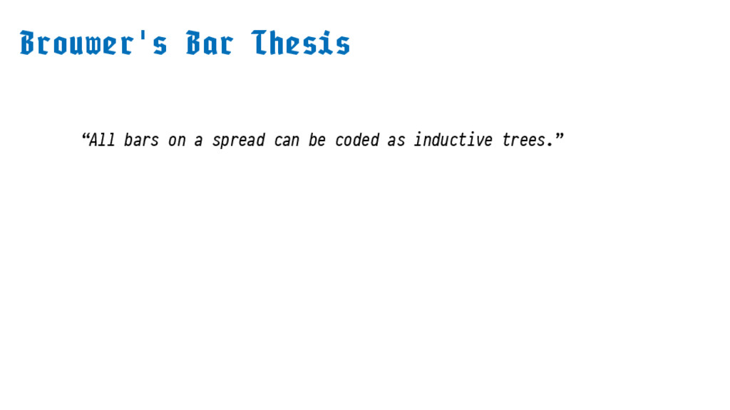
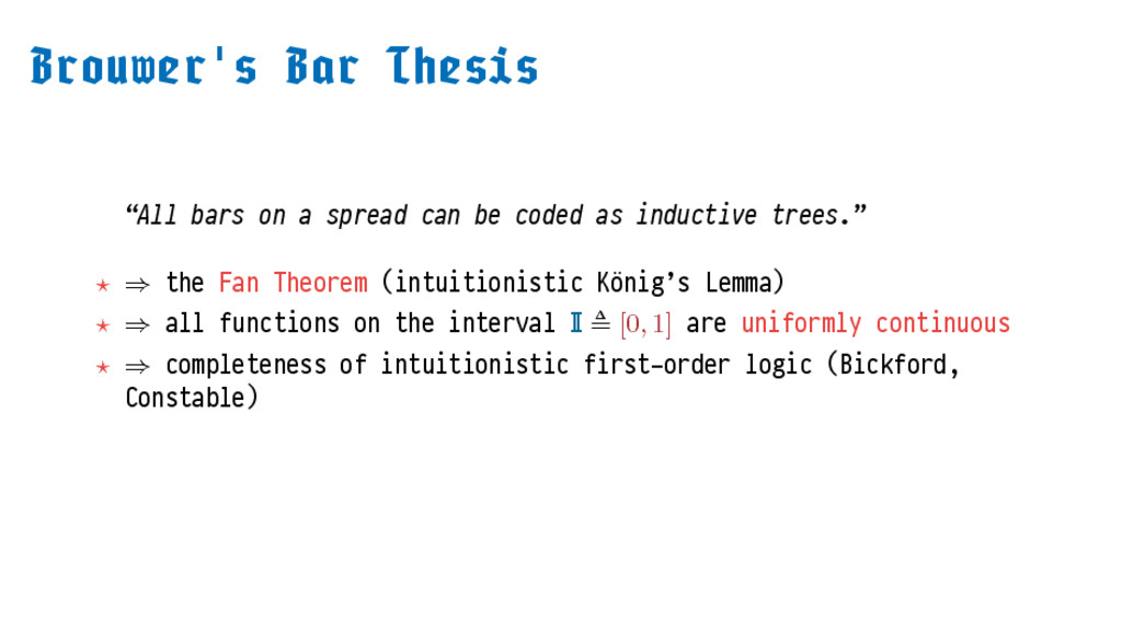
  1. ' “All bars on a spread can be coded as
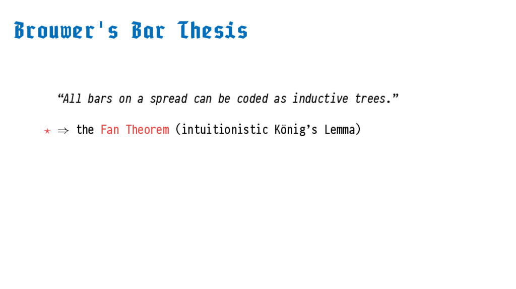
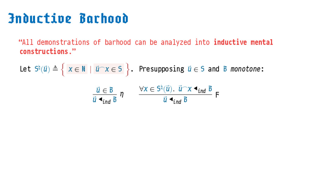
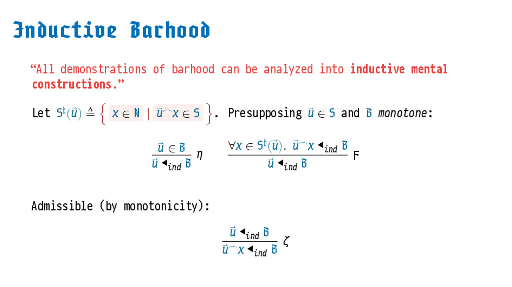
    inductive trees.” ⋆ ⇒ the Fan Theorem (intuitionistic König’s Lemma)
  2. ' “All bars on a spread can be coded as

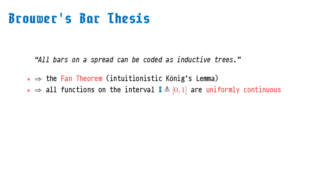
    inductive trees.” ⋆ ⇒ the Fan Theorem (intuitionistic König’s Lemma) ⋆ ⇒ all functions on the interval ≜ [0, 1] are uniformly continuous
  3. ' “All bars on a spread can be coded as

    inductive trees.” ⋆ ⇒ the Fan Theorem (intuitionistic König’s Lemma) ⋆ ⇒ all functions on the interval ≜ [0, 1] are uniformly continuous ⋆ ⇒ completeness of intuitionistic first-order logic (Bickford, Constable)
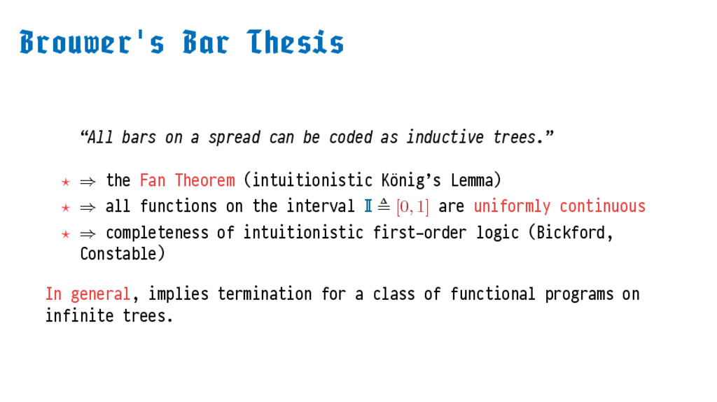
  4. ' “All bars on a spread can be coded as

    inductive trees.” ⋆ ⇒ the Fan Theorem (intuitionistic König’s Lemma) ⋆ ⇒ all functions on the interval ≜ [0, 1] are uniformly continuous ⋆ ⇒ completeness of intuitionistic first-order logic (Bickford, Constable) In general, implies termination for a class of functional programs on infinite trees.
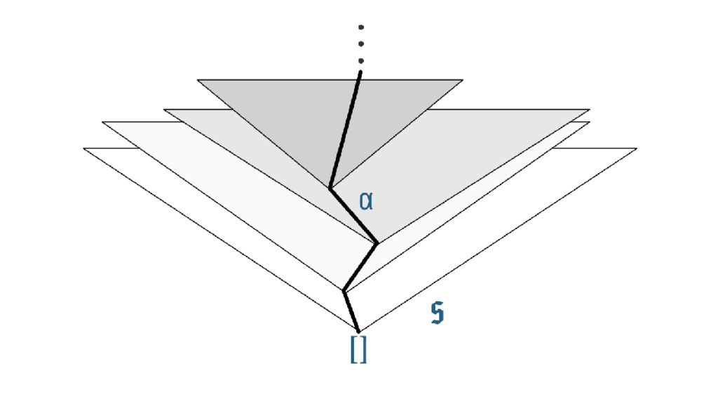
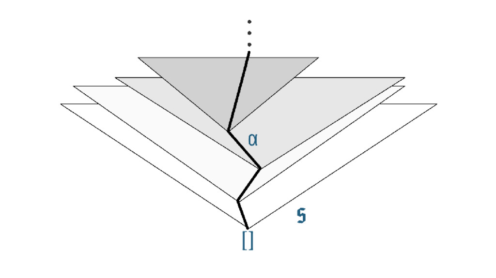
  5. A is at the same time a topological space and

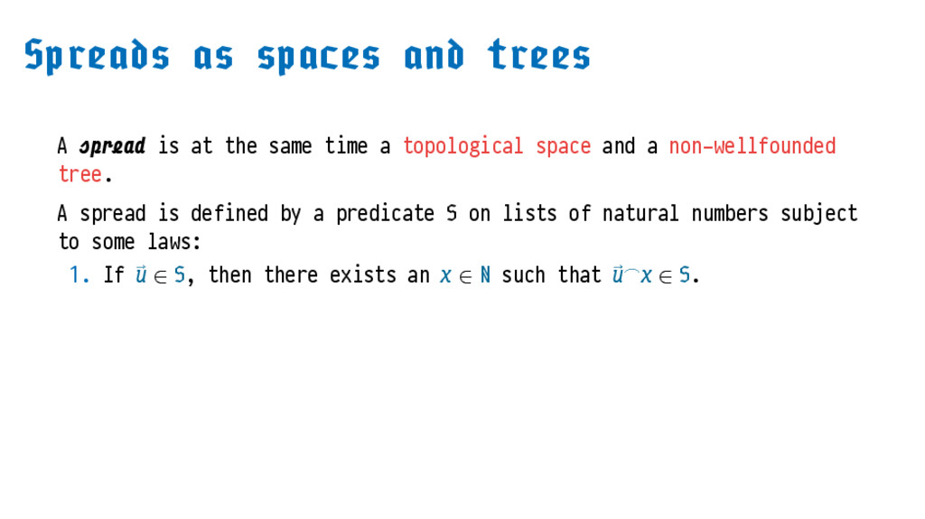
    a non-wellfounded tree. A spread is defined by a predicate on lists of natural numbers subject to some laws:
  6. A is at the same time a topological space and

    a non-wellfounded tree. A spread is defined by a predicate on lists of natural numbers subject to some laws: 1. If ⃗ ∈ , then there exists an ∈ ℕ such that ⃗ ⌢ ∈ .
  7. A is at the same time a topological space and

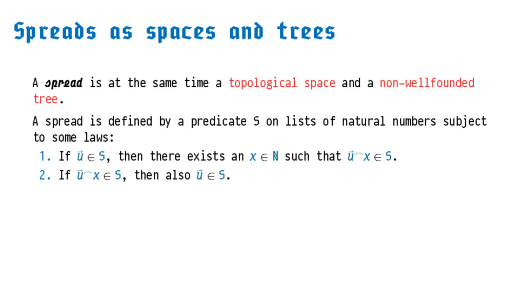
    a non-wellfounded tree. A spread is defined by a predicate on lists of natural numbers subject to some laws: 1. If ⃗ ∈ , then there exists an ∈ ℕ such that ⃗ ⌢ ∈ . 2. If ⃗ ⌢ ∈ , then also ⃗ ∈ .
  8. A is at the same time a topological space and

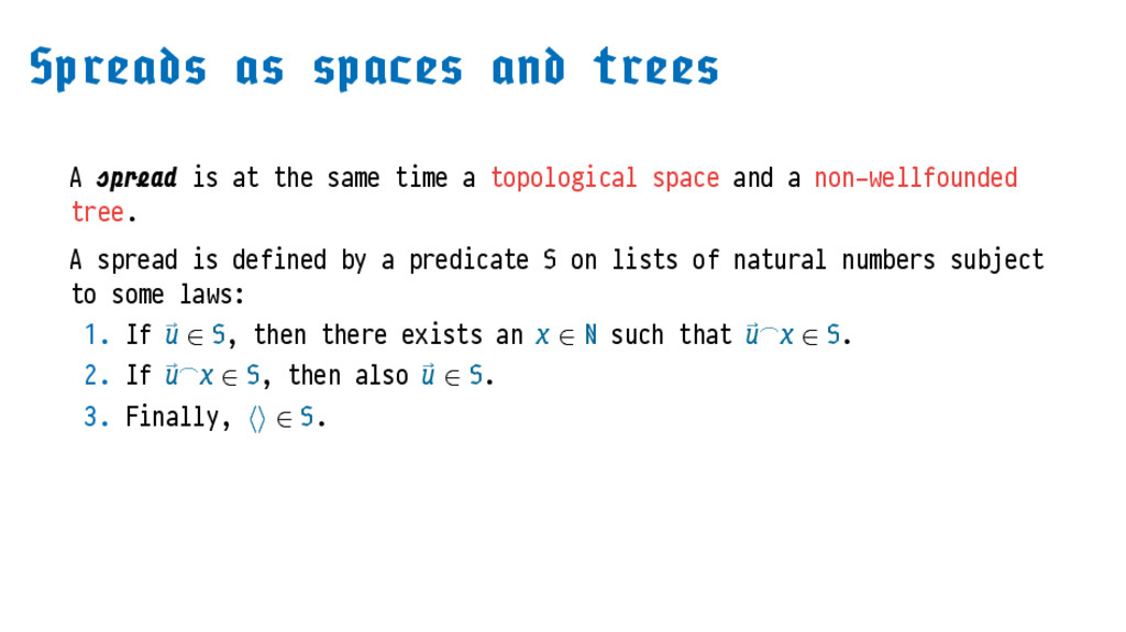
    a non-wellfounded tree. A spread is defined by a predicate on lists of natural numbers subject to some laws: 1. If ⃗ ∈ , then there exists an ∈ ℕ such that ⃗ ⌢ ∈ . 2. If ⃗ ⌢ ∈ , then also ⃗ ∈ . 3. Finally, ⟨⟩ ∈ .
  9. A is at the same time a topological space and

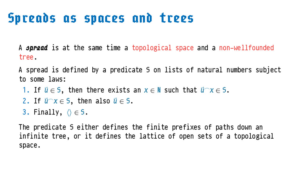
    a non-wellfounded tree. A spread is defined by a predicate on lists of natural numbers subject to some laws: 1. If ⃗ ∈ , then there exists an ∈ ℕ such that ⃗ ⌢ ∈ . 2. If ⃗ ⌢ ∈ , then also ⃗ ∈ . 3. Finally, ⟨⟩ ∈ . The predicate either defines the finite prefixes of paths down an infinite tree, or it defines the lattice of open sets of a topological space.
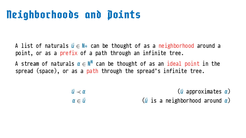
  10. A list of naturals ⃗ ∈ ℕ∗ can be thought

    of as a neighborhood around a point, or as a prefix of a path through an infinite tree. A stream of naturals ∈ ℕℕ can be thought of as an ideal point in the spread (space), or as a path through the spread’s infinite tree. ⃗ ≺ ( ⃗ approximates ) ∈ ⃗ ( ⃗ is a neighborhood around )
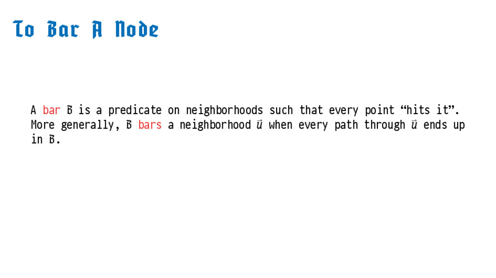
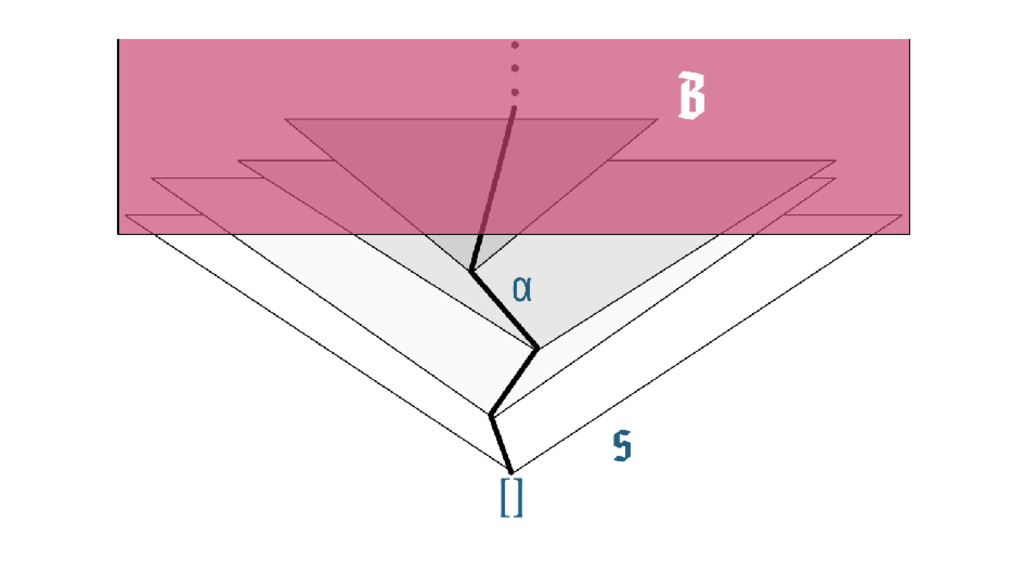
  11. A bar is a predicate on neighborhoods such that every

    point “hits it”. More generally, bars a neighborhood ⃗ when every path through ⃗ ends up in .
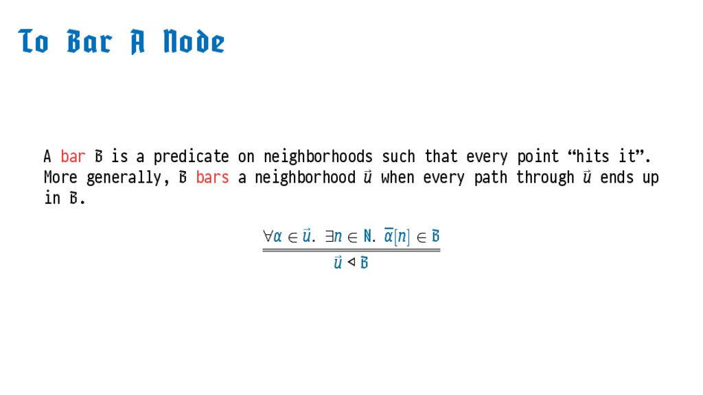
  12. A bar is a predicate on neighborhoods such that every

    point “hits it”. More generally, bars a neighborhood ⃗ when every path through ⃗ ends up in . ∀ ∈ ⃗ . ∃ ∈ ℕ. [] ∈ ⃗ ◁
  13. “All demonstrations of barhood can be analyzed into inductive mental

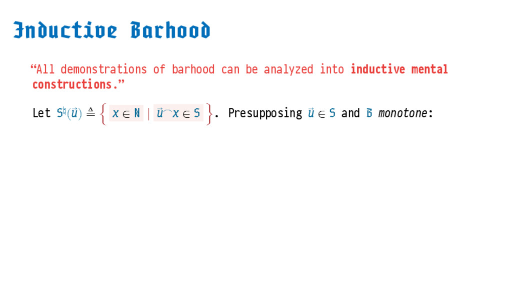
    constructions.” Let ♮( ⃗ ) ≜ { ∈ ℕ ∣ ⃗ ⌢ ∈ }. Presupposing ⃗ ∈ and monotone:
  14. “All demonstrations of barhood can be analyzed into inductive mental

    constructions.” Let ♮( ⃗ ) ≜ { ∈ ℕ ∣ ⃗ ⌢ ∈ }. Presupposing ⃗ ∈ and monotone: ⃗ ∈ ⃗ ◀ ∀ ∈ ♮( ⃗ ). ⃗ ⌢ ◀ ⃗ ◀ ϝ
  15. “All demonstrations of barhood can be analyzed into inductive mental

    constructions.” Let ♮( ⃗ ) ≜ { ∈ ℕ ∣ ⃗ ⌢ ∈ }. Presupposing ⃗ ∈ and monotone: ⃗ ∈ ⃗ ◀ ∀ ∈ ♮( ⃗ ). ⃗ ⌢ ◀ ⃗ ◀ ϝ Admissible (by monotonicity): ⃗ ◀ ⃗ ⌢ ◀
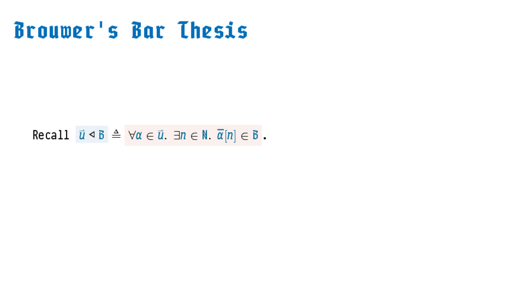
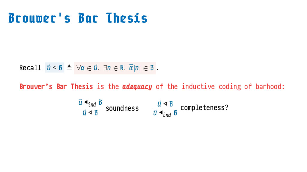
  16. ' Recall ⃗ ◁ ≜ ∀ ∈ ⃗ . ∃

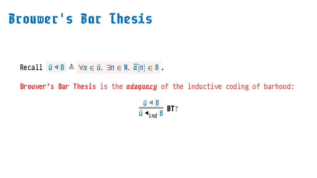
    ∈ ℕ. [] ∈ . Brouwer’s Bar Thesis is the of the inductive coding of barhood: ⃗ ◁ ⃗ ◀ BT?
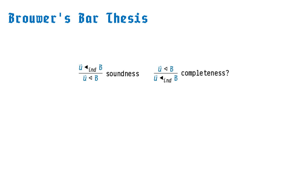
  17. ' Recall ⃗ ◁ ≜ ∀ ∈ ⃗ . ∃

    ∈ ℕ. [] ∈ . Brouwer’s Bar Thesis is the of the inductive coding of barhood: ⃗ ◀ ⃗ ◁ soundness ⃗ ◁ ⃗ ◀ completeness?
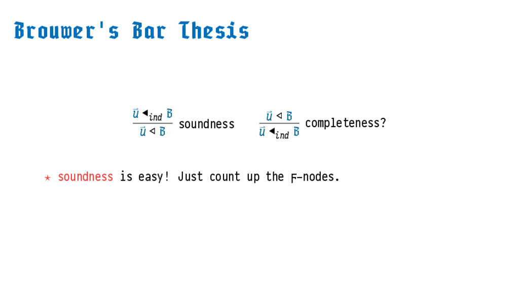
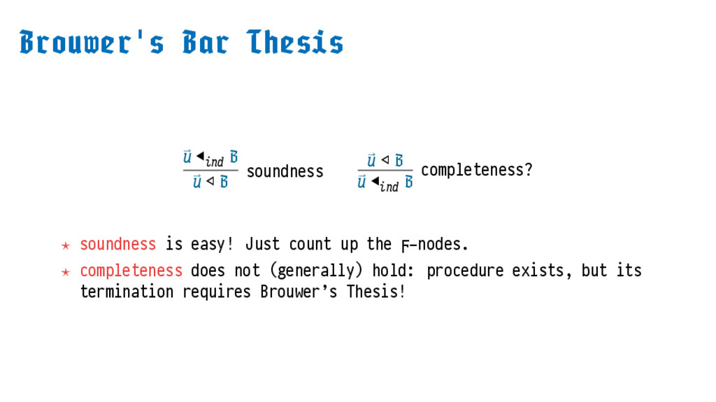
  18. ' ⃗ ◀ ⃗ ◁ soundness ⃗ ◁ ⃗ ◀

    completeness? ⋆ soundness is easy! Just count up the ϝ-nodes.
  19. ' ⃗ ◀ ⃗ ◁ soundness ⃗ ◁ ⃗ ◀

    completeness? ⋆ soundness is easy! Just count up the ϝ-nodes. ⋆ completeness does not (generally) hold: procedure exists, but its termination requires Brouwer’s Thesis!
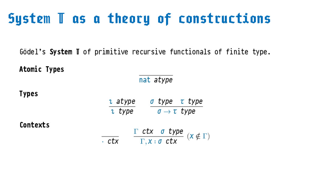
  20. Gödel’s System of primitive recursive functionals of finite type. Atomic

    Types nat atype Types atype type type type → type Contexts ⋅ ctx Γ ctx type Γ, ∶ ctx ( ∉ Γ)
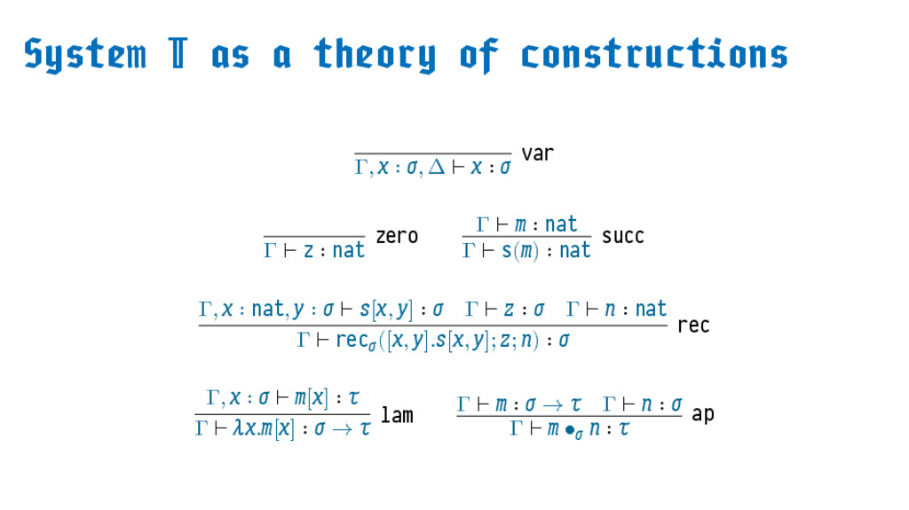
  21. Γ, ∶ , Δ ⊢ ∶ var Γ ⊢ z

    ∶ nat zero Γ ⊢ ∶ nat Γ ⊢ s() ∶ nat succ Γ, ∶ nat, ∶ ⊢ [, ] ∶ Γ ⊢ ∶ Γ ⊢ ∶ nat Γ ⊢ rec ([, ].[, ]; ; ) ∶ rec Γ, ∶ ⊢ [] ∶ Γ ⊢ .[] ∶ → lam Γ ⊢ ∶ → Γ ⊢ ∶ Γ ⊢ • ∶ ap
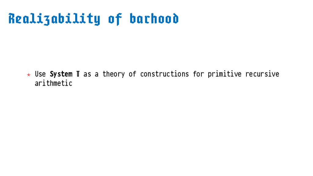
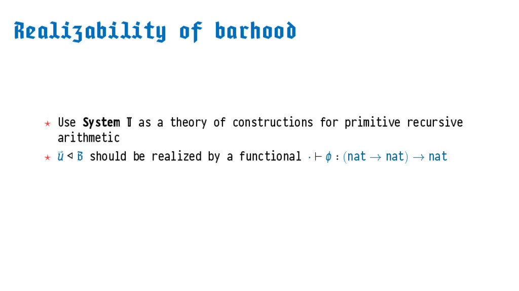
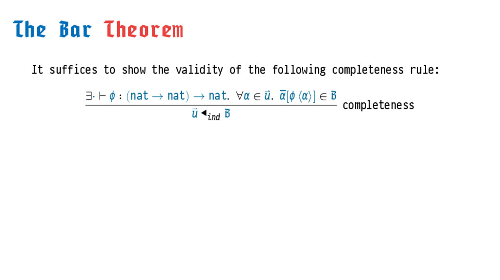
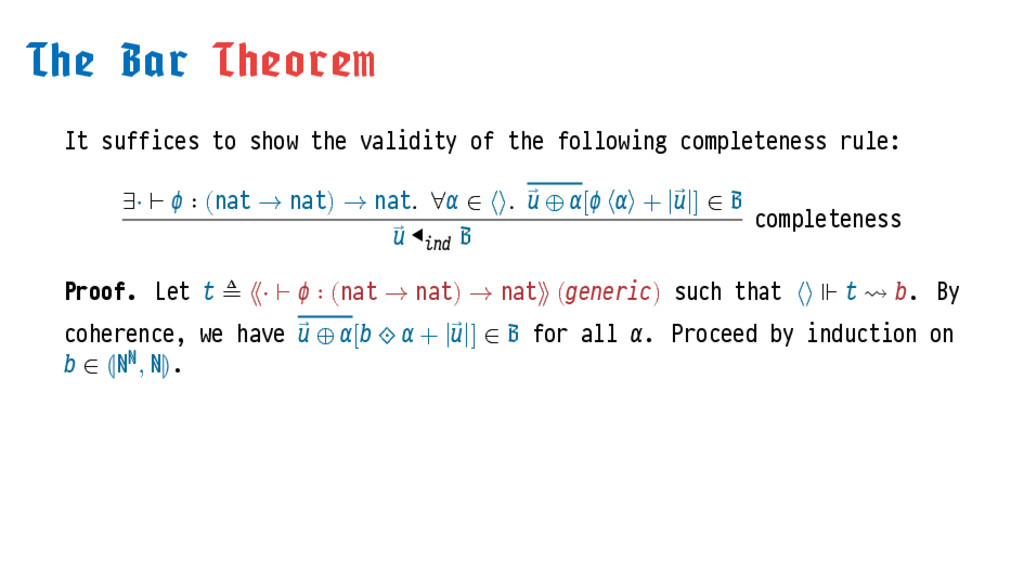
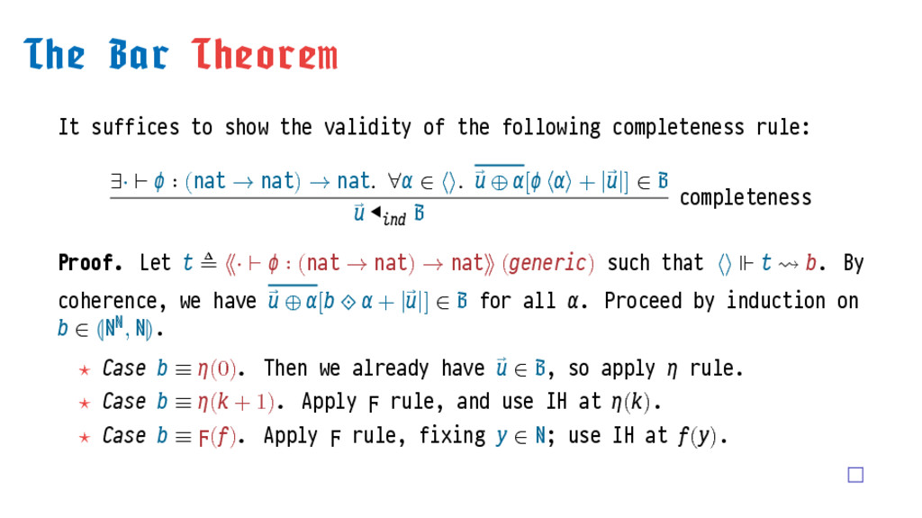
  22. ⋆ Use System as a theory of constructions for primitive

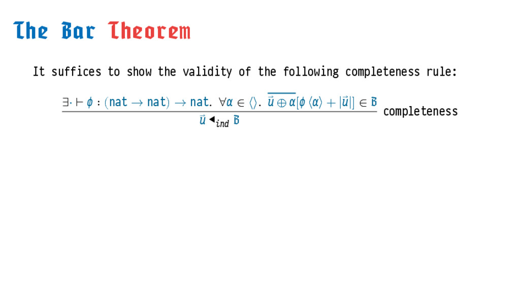
    recursive arithmetic ⋆ ⃗ ◁ should be realized by a functional ⋅ ⊢ ∶ (nat → nat) → nat
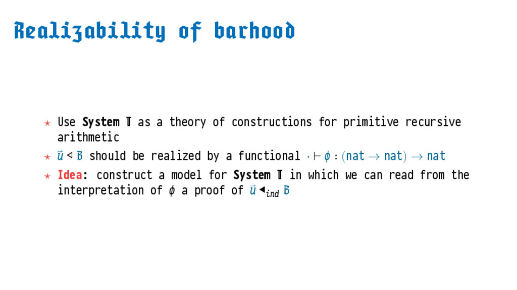
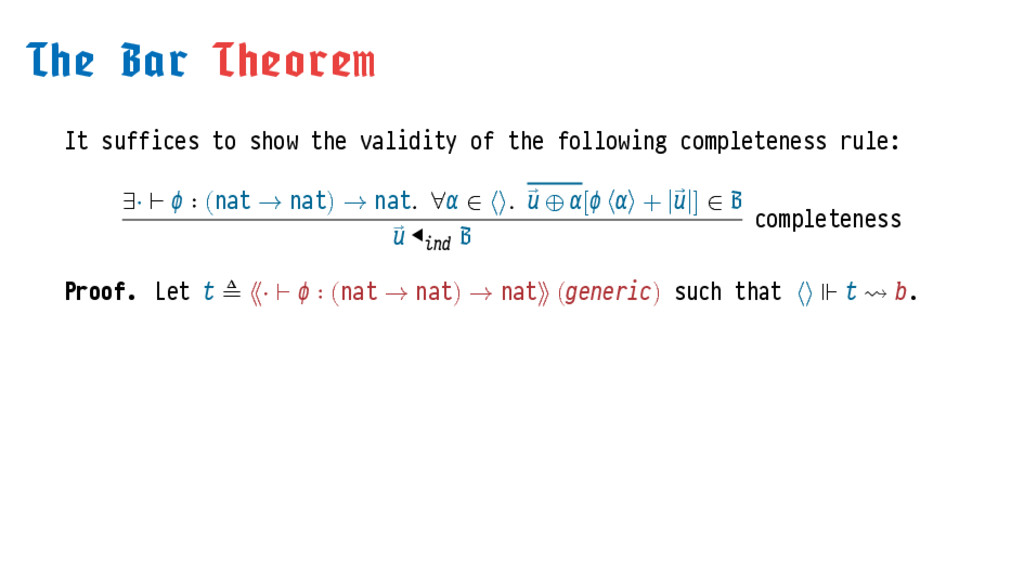
  23. ⋆ Use System as a theory of constructions for primitive

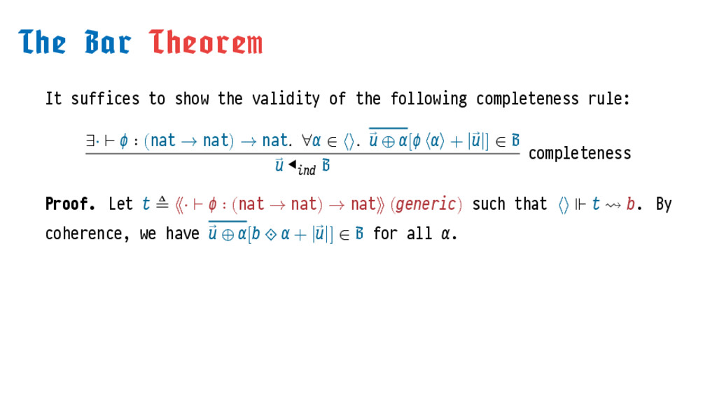
    recursive arithmetic ⋆ ⃗ ◁ should be realized by a functional ⋅ ⊢ ∶ (nat → nat) → nat ⋆ Idea: construct a model for System in which we can read from the interpretation of a proof of ⃗ ◀
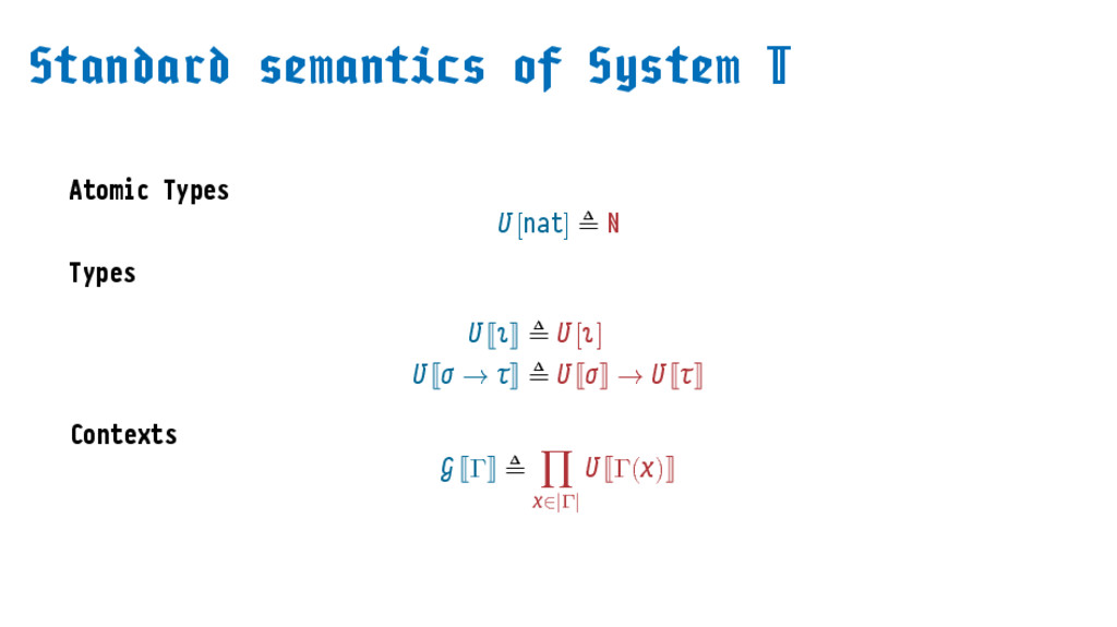
  24. Atomic Types [nat] ≜ ℕ Types ≜ [] → ≜

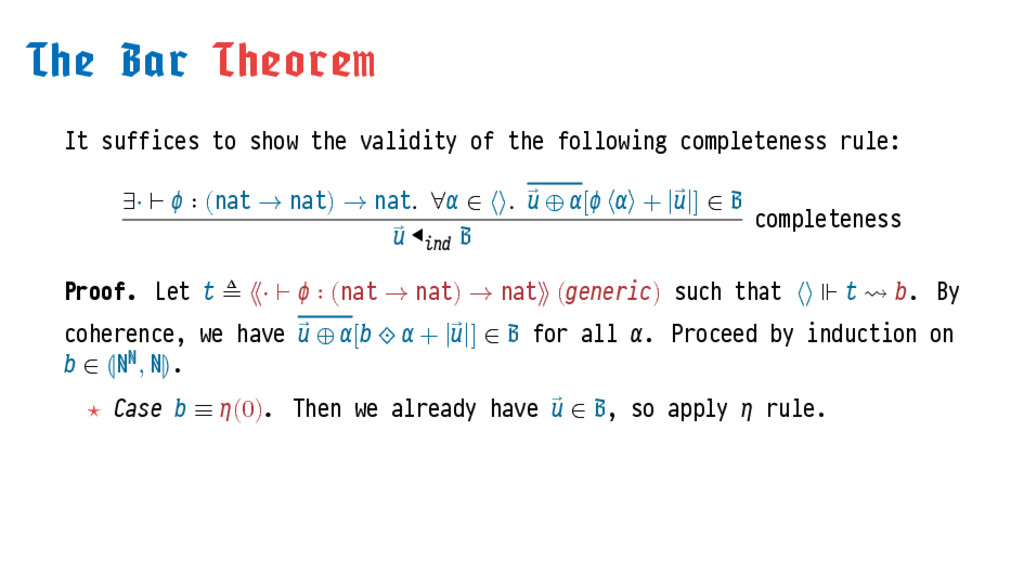
    → Contexts Γ ≜ ∏ ∈|Γ| Γ()
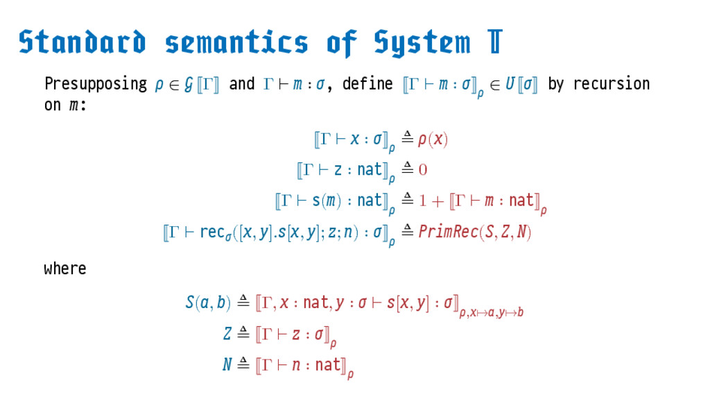
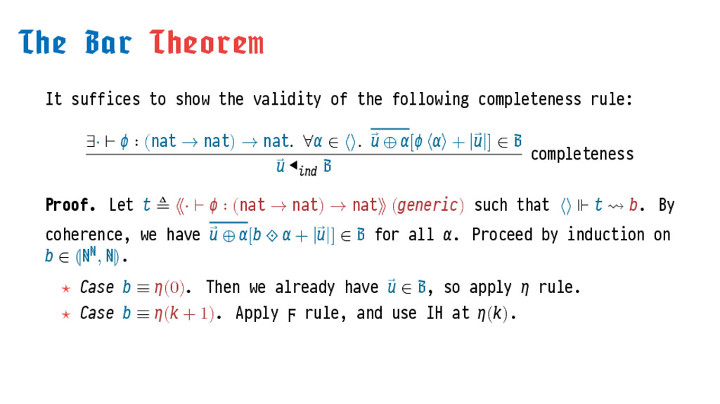
  25. Presupposing ∈ Γ and Γ ⊢ ∶ , define Γ

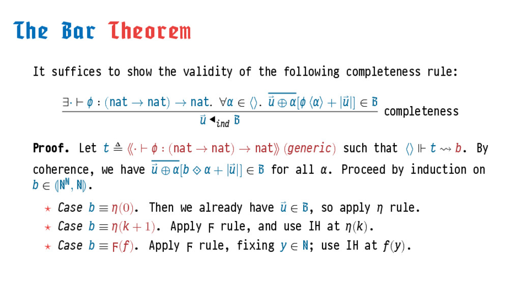
    ⊢ ∶ ∈ by recursion on : Γ ⊢ ∶ ≜ () Γ ⊢ z ∶ nat ≜ 0 Γ ⊢ s() ∶ nat ≜ 1 + Γ ⊢ ∶ nat Γ ⊢ rec ([, ].[, ]; ; ) ∶ ≜ PrimRec(, , ) where (, ) ≜ Γ, ∶ nat, ∶ ⊢ [, ] ∶ ,↦,↦ ≜ Γ ⊢ ∶ ≜ Γ ⊢ ∶ nat
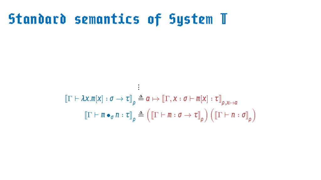
  26. ⋮ Γ ⊢ .[] ∶ → ≜ ↦ Γ, ∶

    ⊢ [] ∶ ,↦ Γ ⊢ • ∶ ≜ ( Γ ⊢ ∶ → ) ( Γ ⊢ ∶ )
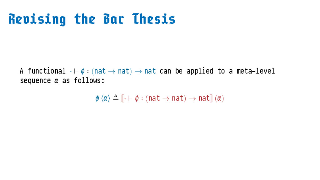
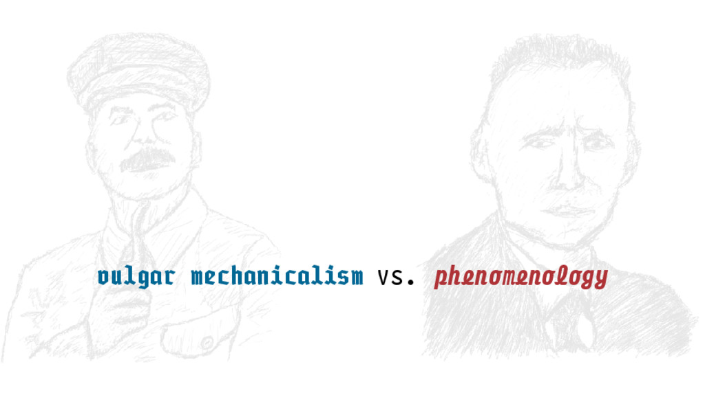
  27. A functional ⋅ ⊢ ∶ (nat → nat) → nat

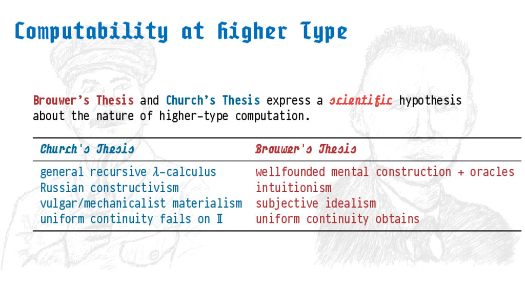
    can be applied to a meta-level sequence as follows: ⟨⟩ ≜ ⋅ ⊢ ∶ (nat → nat) → nat ()
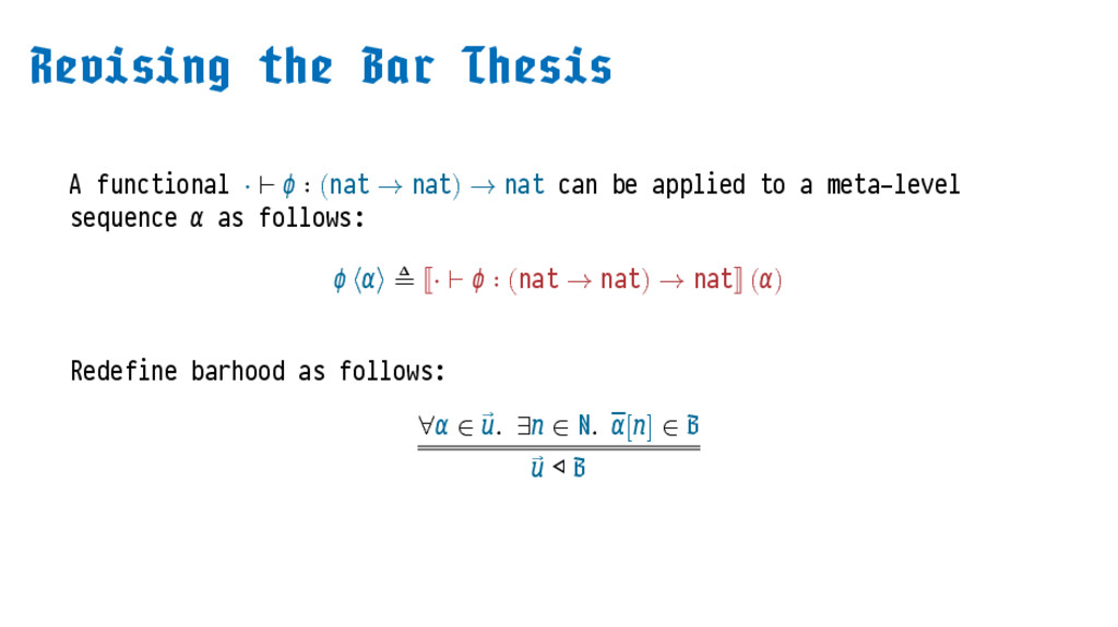
  28. A functional ⋅ ⊢ ∶ (nat → nat) → nat

    can be applied to a meta-level sequence as follows: ⟨⟩ ≜ ⋅ ⊢ ∶ (nat → nat) → nat () Redefine barhood as follows: ∀ ∈ ⃗ . ∃ ∈ ℕ. [] ∈ ⃗ ◁
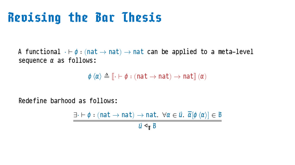
  29. A functional ⋅ ⊢ ∶ (nat → nat) → nat

    can be applied to a meta-level sequence as follows: ⟨⟩ ≜ ⋅ ⊢ ∶ (nat → nat) → nat () Redefine barhood as follows: ∃⋅ ⊢ ∶ (nat → nat) → nat. ∀ ∈ ⃗ . [ ⟨⟩] ∈ ⃗ ◁
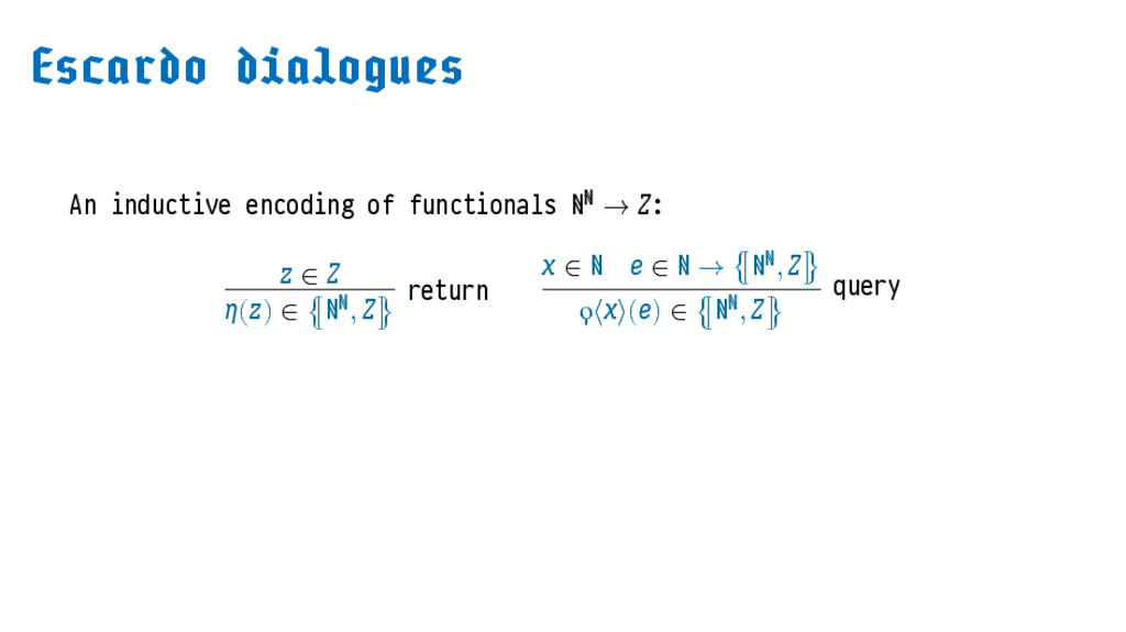
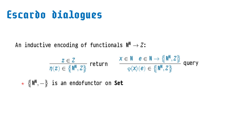
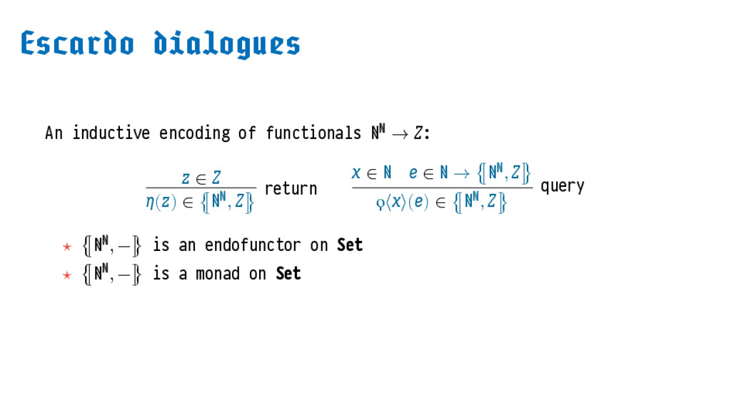
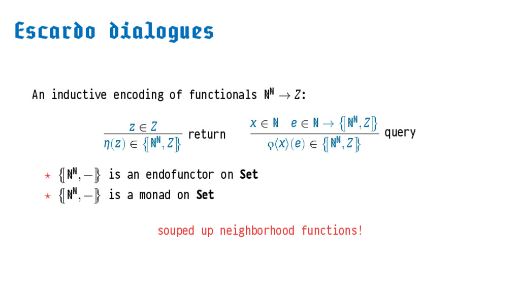
  30. An inductive encoding of functionals ℕℕ → : ∈ ()

    ∈ ⦃ℕℕ, ⦄ return ∈ ℕ ∈ ℕ → ⦃ℕℕ, ⦄ ϙ⟨⟩() ∈ ⦃ℕℕ, ⦄ query
  31. An inductive encoding of functionals ℕℕ → : ∈ ()

    ∈ ⦃ℕℕ, ⦄ return ∈ ℕ ∈ ℕ → ⦃ℕℕ, ⦄ ϙ⟨⟩() ∈ ⦃ℕℕ, ⦄ query ⋆ ⦃ℕℕ, −⦄ is an endofunctor on Set
  32. An inductive encoding of functionals ℕℕ → : ∈ ()

    ∈ ⦃ℕℕ, ⦄ return ∈ ℕ ∈ ℕ → ⦃ℕℕ, ⦄ ϙ⟨⟩() ∈ ⦃ℕℕ, ⦄ query ⋆ ⦃ℕℕ, −⦄ is an endofunctor on Set ⋆ ⦃ℕℕ, −⦄ is a monad on Set
  33. An inductive encoding of functionals ℕℕ → : ∈ ()

    ∈ ⦃ℕℕ, ⦄ return ∈ ℕ ∈ ℕ → ⦃ℕℕ, ⦄ ϙ⟨⟩() ∈ ⦃ℕℕ, ⦄ query ⋆ ⦃ℕℕ, −⦄ is an endofunctor on Set ⋆ ⦃ℕℕ, −⦄ is a monad on Set souped up neighborhood functions!
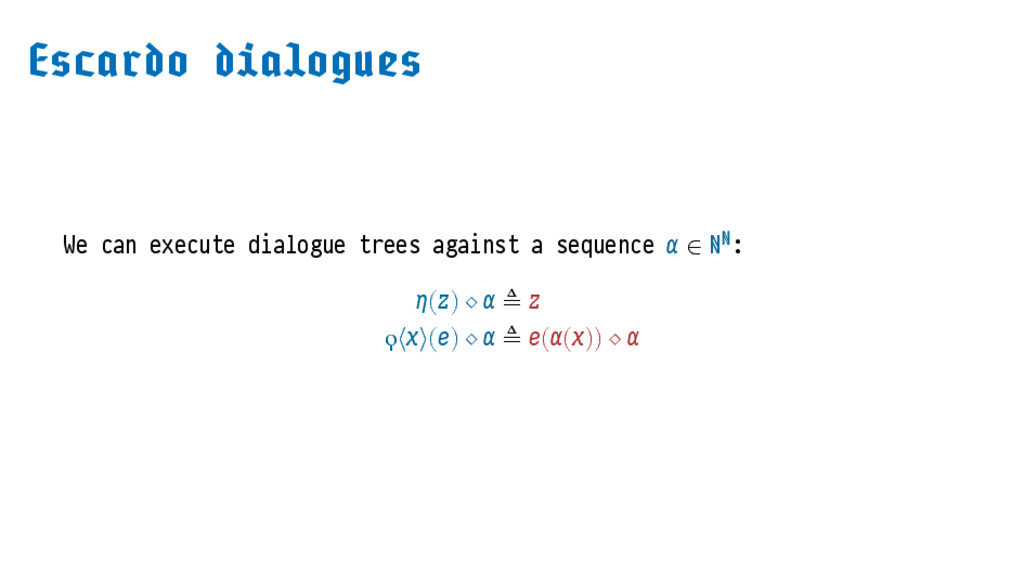
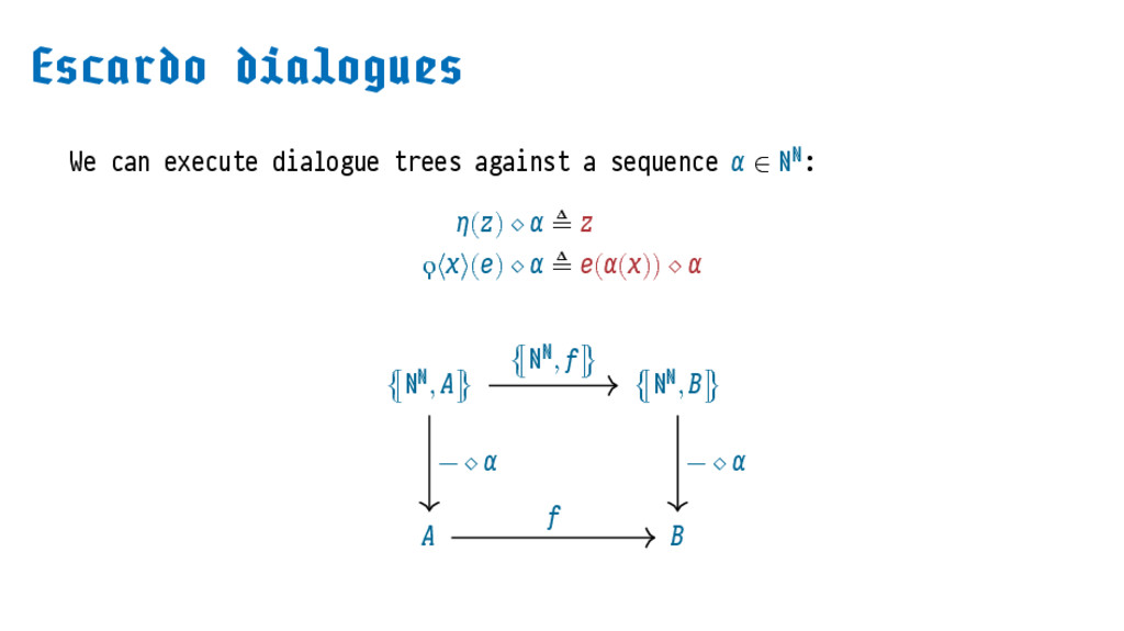
  34. We can execute dialogue trees against a sequence ∈ ℕℕ:

    () ⋄ ≜ ϙ⟨⟩() ⋄ ≜ (()) ⋄
  35. We can execute dialogue trees against a sequence ∈ ℕℕ:

    () ⋄ ≜ ϙ⟨⟩() ⋄ ≜ (()) ⋄ ⦃ℕℕ, ⦄ ⦃ℕℕ, ⦄ ⦃ℕℕ, ⦄ − ⋄ − ⋄
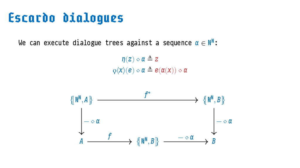
  36. We can execute dialogue trees against a sequence ∈ ℕℕ:

    () ⋄ ≜ ϙ⟨⟩() ⋄ ≜ (()) ⋄ ⦃ℕℕ, ⦄ ⦃ℕℕ, ⦄ ⦃ℕℕ, ⦄ ⋆ − ⋄ − ⋄ − ⋄
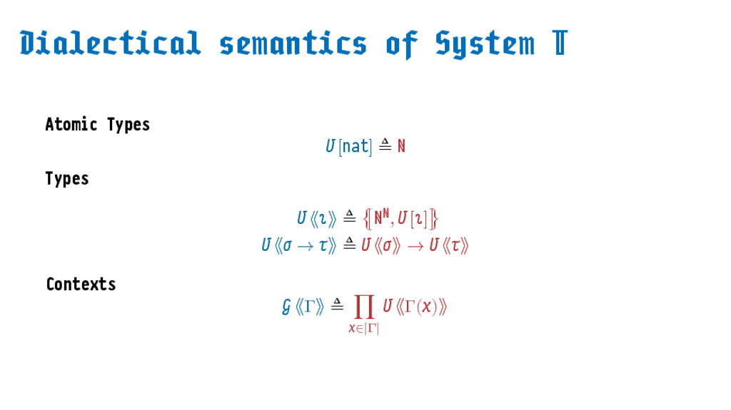
  37. Atomic Types [nat] ≜ ℕ Types ⟪⟫ ≜ ⦃ℕℕ, []⦄

    ⟪ → ⟫ ≜ ⟪⟫ → ⟪⟫ Contexts ⟪Γ⟫ ≜ ∏ ∈|Γ| ⟪Γ()⟫
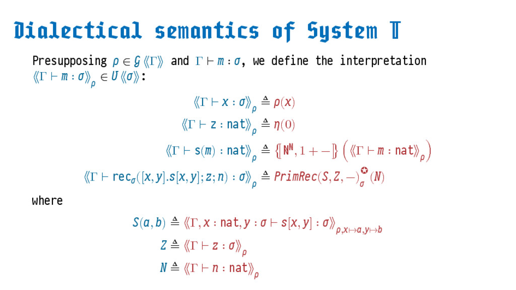
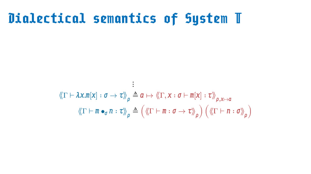
  38. Presupposing ∈ ⟪Γ⟫ and Γ ⊢ ∶ , we define

    the interpretation ⟪Γ ⊢ ∶ ⟫ ∈ ⟪⟫: ⟪Γ ⊢ ∶ ⟫ ≜ () ⟪Γ ⊢ z ∶ nat⟫ ≜ (0) ⟪Γ ⊢ s() ∶ nat⟫ ≜ ⦃ℕℕ, 1 + −⦄ (⟪Γ ⊢ ∶ nat⟫ ) ⟪Γ ⊢ rec ([, ].[, ]; ; ) ∶ ⟫ ≜ PrimRec(, , −)✪ () where (, ) ≜ ⟪Γ, ∶ nat, ∶ ⊢ [, ] ∶ ⟫ ,↦,↦ ≜ ⟪Γ ⊢ ∶ ⟫ ≜ ⟪Γ ⊢ ∶ nat⟫
  39. ⋮ ⟪Γ ⊢ .[] ∶ → ⟫ ≜ ↦ ⟪Γ,

    ∶ ⊢ [] ∶ ⟫ ,↦ ⟪Γ ⊢ • ∶ ⟫ ≜ (⟪Γ ⊢ ∶ → ⟫ ) (⟪Γ ⊢ ∶ ⟫ )
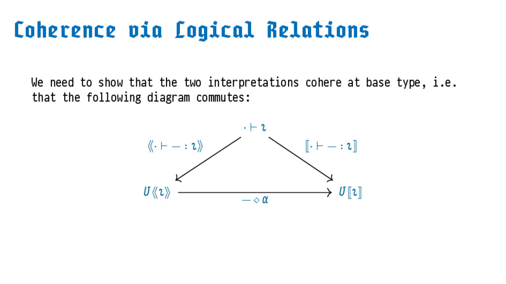
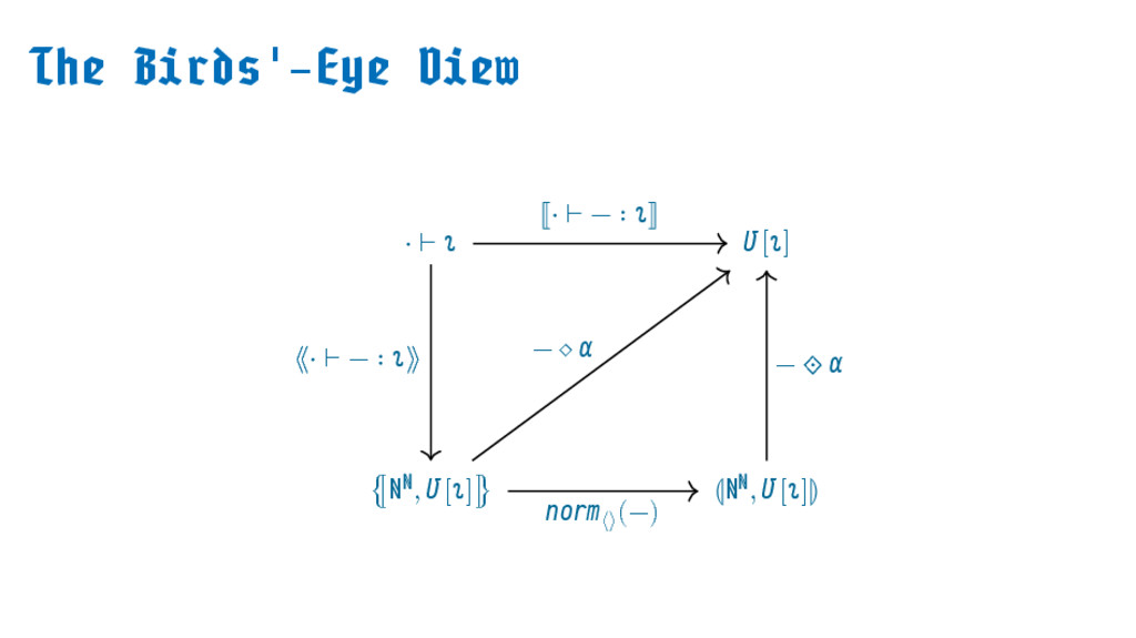
  40. We need to show that the two interpretations cohere at

    base type, i.e. that the following diagram commutes: ⋅ ⊢ ⟪⟫ ⟪⋅ ⊢ − ∶ ⟫ ⋅ ⊢ − ∶ − ⋄
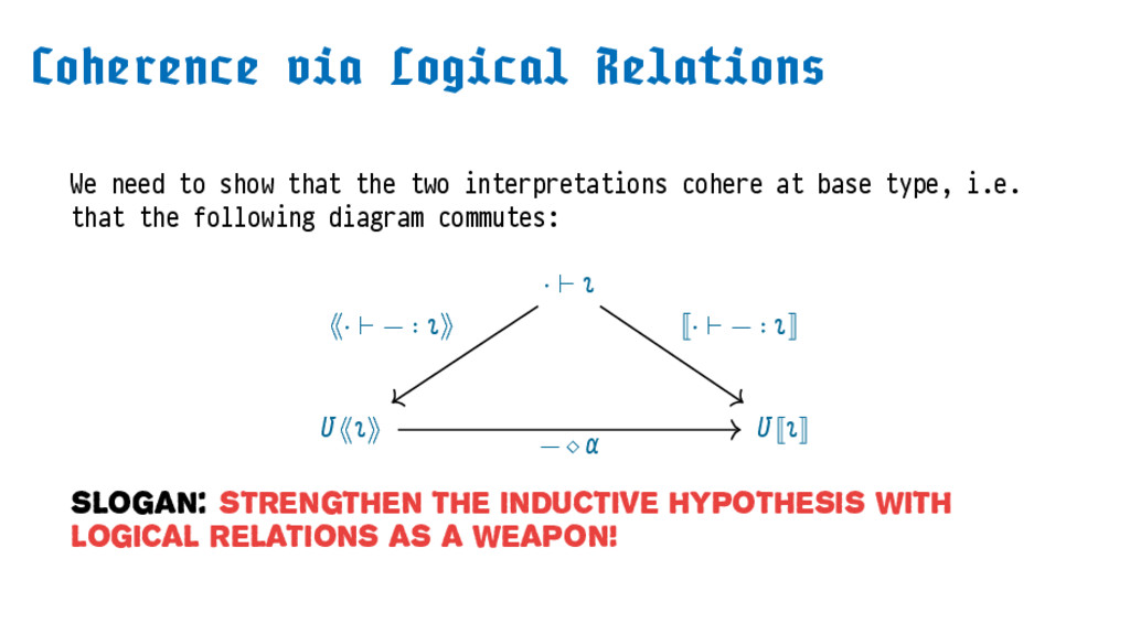
  41. We need to show that the two interpretations cohere at

    base type, i.e. that the following diagram commutes: ⋅ ⊢ ⟪⟫ ⟪⋅ ⊢ − ∶ ⟫ ⋅ ⊢ − ∶ − ⋄ Slogan: Strengthen The Inductive Hypothesis With Logical Relations As A Weapon!
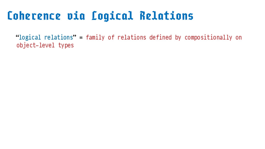
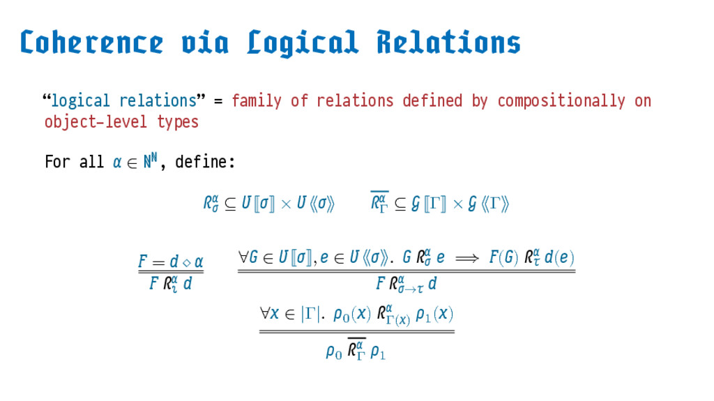
  42. “logical relations” = family of relations defined by compositionally on

    object-level types For all ∈ ℕℕ, define: ℛ ⊆ × ⟪⟫ ℛ Γ ⊆ Γ × ⟪Γ⟫ = ⋄ ℛ ∀ ∈ , ∈ ⟪⟫. ℛ ⟹ () ℛ () ℛ → ∀ ∈ |Γ|. 0 () ℛ Γ() 1 () 0 ℛ Γ 1
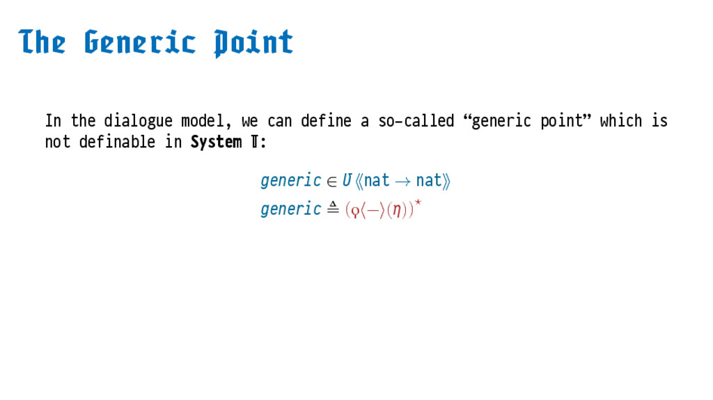
  43. In the dialogue model, we can define a so-called “generic

    point” which is not definable in System : generic ∈ ⟪nat → nat⟫ generic ≜ (ϙ⟨−⟩())⋆
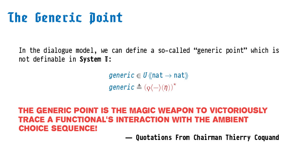
  44. In the dialogue model, we can define a so-called “generic

    point” which is not definable in System : generic ∈ ⟪nat → nat⟫ generic ≜ (ϙ⟨−⟩())⋆ The Generic Point Is The Magic Weapon To Victoriously Trace A Functional's Interaction With The Ambient Choice Sequence! — Quotations From Chairman Thierry Coquand
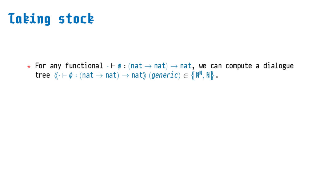
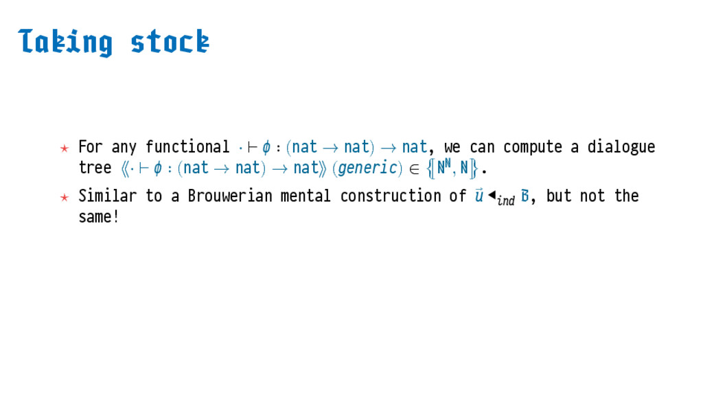
  45. ⋆ For any functional ⋅ ⊢ ∶ (nat → nat)

    → nat, we can compute a dialogue tree ⟪⋅ ⊢ ∶ (nat → nat) → nat⟫ (generic) ∈ ⦃ℕℕ, ℕ⦄.
  46. ⋆ For any functional ⋅ ⊢ ∶ (nat → nat)

    → nat, we can compute a dialogue tree ⟪⋅ ⊢ ∶ (nat → nat) → nat⟫ (generic) ∈ ⦃ℕℕ, ℕ⦄. ⋆ Similar to a Brouwerian mental construction of ⃗ ◀ , but not the same!
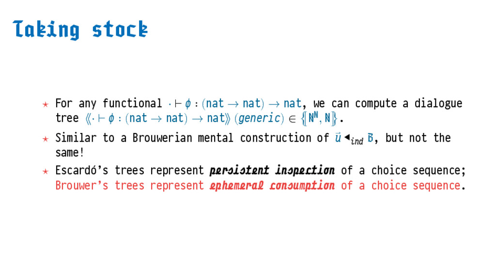
  47. ⋆ For any functional ⋅ ⊢ ∶ (nat → nat)

    → nat, we can compute a dialogue tree ⟪⋅ ⊢ ∶ (nat → nat) → nat⟫ (generic) ∈ ⦃ℕℕ, ℕ⦄. ⋆ Similar to a Brouwerian mental construction of ⃗ ◀ , but not the same! ⋆ Escardó’s trees represent of a choice sequence; Brouwer’s trees represent of a choice sequence.
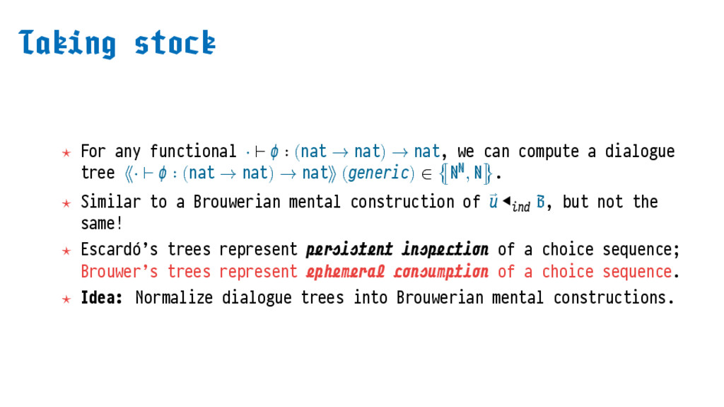
  48. ⋆ For any functional ⋅ ⊢ ∶ (nat → nat)

    → nat, we can compute a dialogue tree ⟪⋅ ⊢ ∶ (nat → nat) → nat⟫ (generic) ∈ ⦃ℕℕ, ℕ⦄. ⋆ Similar to a Brouwerian mental construction of ⃗ ◀ , but not the same! ⋆ Escardó’s trees represent of a choice sequence; Brouwer’s trees represent of a choice sequence. ⋆ Idea: Normalize dialogue trees into Brouwerian mental constructions.
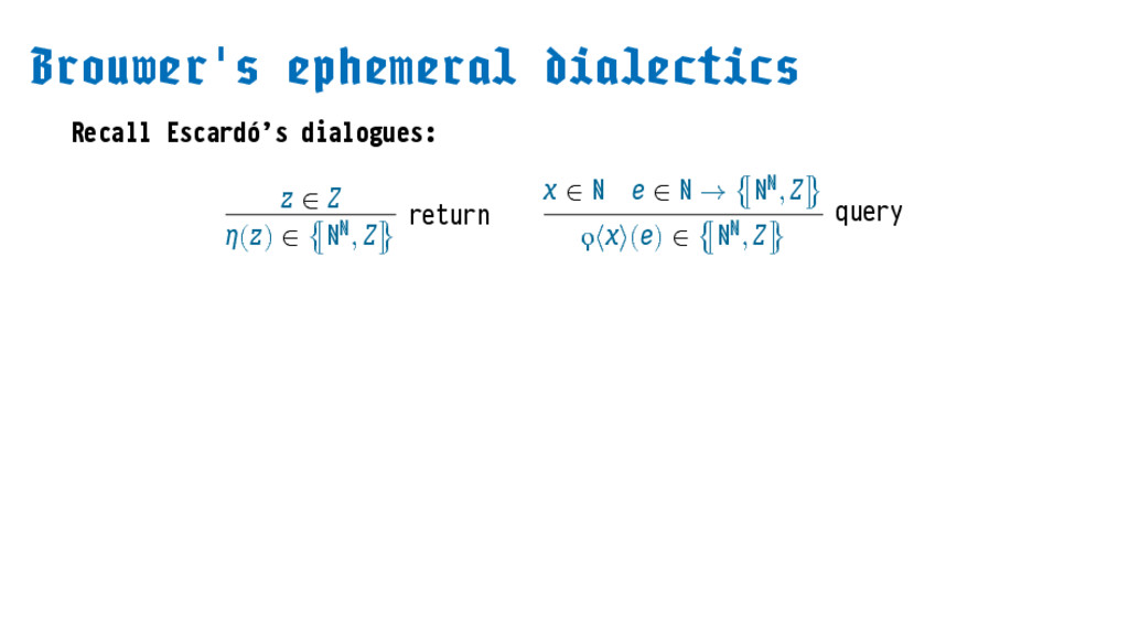
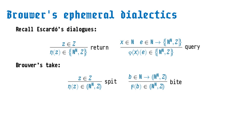
  49. ' Recall Escardó’s dialogues: ∈ () ∈ ⦃ℕℕ, ⦄ return

    ∈ ℕ ∈ ℕ → ⦃ℕℕ, ⦄ ϙ⟨⟩() ∈ ⦃ℕℕ, ⦄ query
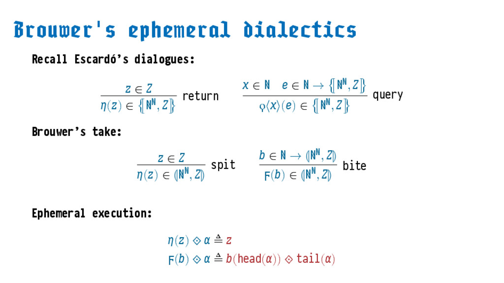
  50. ' Recall Escardó’s dialogues: ∈ () ∈ ⦃ℕℕ, ⦄ return

    ∈ ℕ ∈ ℕ → ⦃ℕℕ, ⦄ ϙ⟨⟩() ∈ ⦃ℕℕ, ⦄ query Brouwer’s take: ∈ () ∈ ℕℕ, spit ∈ ℕ → ℕℕ, ϝ() ∈ ℕℕ, bite
  51. ' Recall Escardó’s dialogues: ∈ () ∈ ⦃ℕℕ, ⦄ return

    ∈ ℕ ∈ ℕ → ⦃ℕℕ, ⦄ ϙ⟨⟩() ∈ ⦃ℕℕ, ⦄ query Brouwer’s take: ∈ () ∈ ℕℕ, spit ∈ ℕ → ℕℕ, ϝ() ∈ ℕℕ, bite Ephemeral execution: () ⟐ ≜ ϝ() ⟐ ≜ (head()) ⟐ tail()
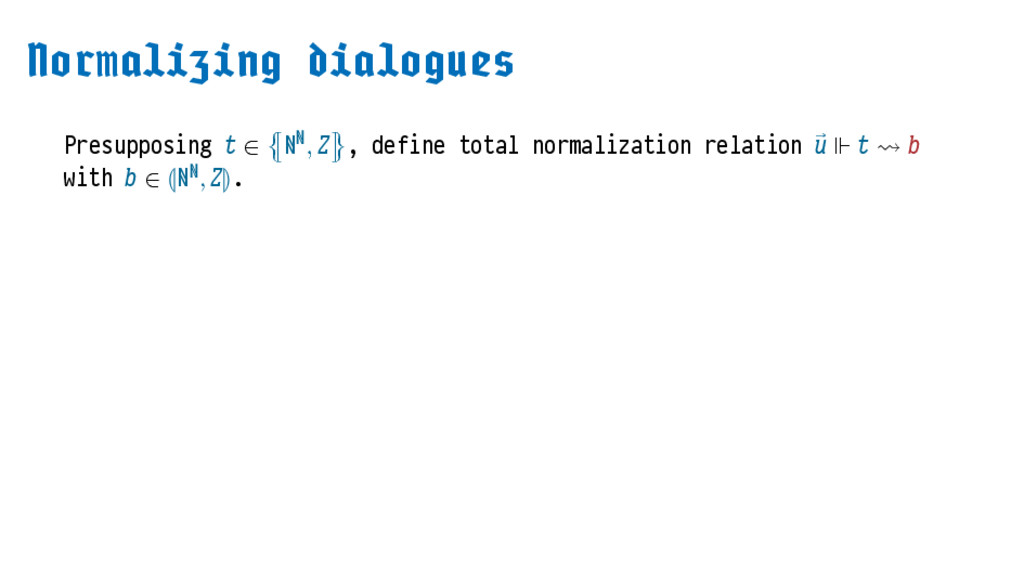
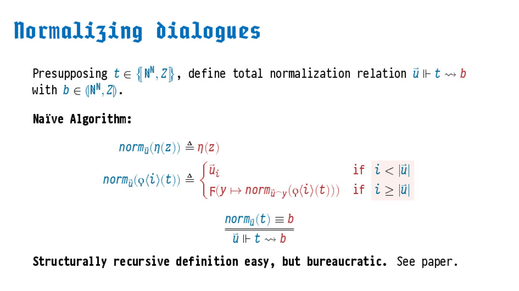
  52. Presupposing ∈ ⦃ℕℕ, ⦄, define total normalization relation ⃗ ⊩

    with ∈ ℕℕ, . Naïve Algorithm: norm ⃗ (()) ≜ () norm ⃗ (ϙ⟨⟩()) ≜ { ⃗ if < | ⃗ | ϝ( ↦ norm ⃗ ⌢ (ϙ⟨⟩())) if ≥ | ⃗ | norm ⃗ () ≡ ⃗ ⊩ Structurally recursive definition easy, but bureaucratic. See paper.
  53. '- ⋅ ⊢ [] ⦃ℕℕ, []⦄ ℕℕ, [] ⋅ ⊢

    − ∶ ⟪⋅ ⊢ − ∶ ⟫ − ⋄ norm⟨⟩ (−) − ⟐
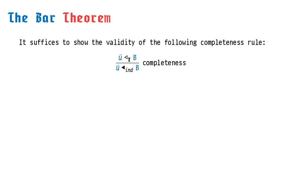
  54. It suffices to show the validity of the following completeness

    rule: ∃⋅ ⊢ ∶ (nat → nat) → nat. ∀ ∈ ⃗ . [ ⟨⟩] ∈ ⃗ ◀ completeness
  55. It suffices to show the validity of the following completeness

    rule: ∃⋅ ⊢ ∶ (nat → nat) → nat. ∀ ∈ ⟨⟩. ⃗ ⊕ [ ⟨⟩ + | ⃗ |] ∈ ⃗ ◀ completeness
  56. It suffices to show the validity of the following completeness

    rule: ∃⋅ ⊢ ∶ (nat → nat) → nat. ∀ ∈ ⟨⟩. ⃗ ⊕ [ ⟨⟩ + | ⃗ |] ∈ ⃗ ◀ completeness Proof. Let ≜ ⟪⋅ ⊢ ∶ (nat → nat) → nat⟫ (generic) such that ⟨⟩ ⊩ .
  57. It suffices to show the validity of the following completeness

    rule: ∃⋅ ⊢ ∶ (nat → nat) → nat. ∀ ∈ ⟨⟩. ⃗ ⊕ [ ⟨⟩ + | ⃗ |] ∈ ⃗ ◀ completeness Proof. Let ≜ ⟪⋅ ⊢ ∶ (nat → nat) → nat⟫ (generic) such that ⟨⟩ ⊩ . By coherence, we have ⃗ ⊕ [ ⟐ + | ⃗ |] ∈ for all .
  58. It suffices to show the validity of the following completeness

    rule: ∃⋅ ⊢ ∶ (nat → nat) → nat. ∀ ∈ ⟨⟩. ⃗ ⊕ [ ⟨⟩ + | ⃗ |] ∈ ⃗ ◀ completeness Proof. Let ≜ ⟪⋅ ⊢ ∶ (nat → nat) → nat⟫ (generic) such that ⟨⟩ ⊩ . By coherence, we have ⃗ ⊕ [ ⟐ + | ⃗ |] ∈ for all . Proceed by induction on ∈ ℕℕ, ℕ .
  59. It suffices to show the validity of the following completeness

    rule: ∃⋅ ⊢ ∶ (nat → nat) → nat. ∀ ∈ ⟨⟩. ⃗ ⊕ [ ⟨⟩ + | ⃗ |] ∈ ⃗ ◀ completeness Proof. Let ≜ ⟪⋅ ⊢ ∶ (nat → nat) → nat⟫ (generic) such that ⟨⟩ ⊩ . By coherence, we have ⃗ ⊕ [ ⟐ + | ⃗ |] ∈ for all . Proceed by induction on ∈ ℕℕ, ℕ . ⋆ Case ≡ (0). Then we already have ⃗ ∈ , so apply rule.
  60. It suffices to show the validity of the following completeness

    rule: ∃⋅ ⊢ ∶ (nat → nat) → nat. ∀ ∈ ⟨⟩. ⃗ ⊕ [ ⟨⟩ + | ⃗ |] ∈ ⃗ ◀ completeness Proof. Let ≜ ⟪⋅ ⊢ ∶ (nat → nat) → nat⟫ (generic) such that ⟨⟩ ⊩ . By coherence, we have ⃗ ⊕ [ ⟐ + | ⃗ |] ∈ for all . Proceed by induction on ∈ ℕℕ, ℕ . ⋆ Case ≡ (0). Then we already have ⃗ ∈ , so apply rule. ⋆ Case ≡ ( + 1). Apply ϝ rule, and use IH at ().
  61. It suffices to show the validity of the following completeness

    rule: ∃⋅ ⊢ ∶ (nat → nat) → nat. ∀ ∈ ⟨⟩. ⃗ ⊕ [ ⟨⟩ + | ⃗ |] ∈ ⃗ ◀ completeness Proof. Let ≜ ⟪⋅ ⊢ ∶ (nat → nat) → nat⟫ (generic) such that ⟨⟩ ⊩ . By coherence, we have ⃗ ⊕ [ ⟐ + | ⃗ |] ∈ for all . Proceed by induction on ∈ ℕℕ, ℕ . ⋆ Case ≡ (0). Then we already have ⃗ ∈ , so apply rule. ⋆ Case ≡ ( + 1). Apply ϝ rule, and use IH at (). ⋆ Case ≡ ϝ(). Apply ϝ rule, fixing ∈ ℕ; use IH at ().
  62. It suffices to show the validity of the following completeness

    rule: ∃⋅ ⊢ ∶ (nat → nat) → nat. ∀ ∈ ⟨⟩. ⃗ ⊕ [ ⟨⟩ + | ⃗ |] ∈ ⃗ ◀ completeness Proof. Let ≜ ⟪⋅ ⊢ ∶ (nat → nat) → nat⟫ (generic) such that ⟨⟩ ⊩ . By coherence, we have ⃗ ⊕ [ ⟐ + | ⃗ |] ∈ for all . Proceed by induction on ∈ ℕℕ, ℕ . ⋆ Case ≡ (0). Then we already have ⃗ ∈ , so apply rule. ⋆ Case ≡ ( + 1). Apply ϝ rule, and use IH at (). ⋆ Case ≡ ϝ(). Apply ϝ rule, fixing ∈ ℕ; use IH at ().
  63. ⋆ The Bar Theorem is in primitive recursive realizability (with

    correct/full interpretation of functional types). ⋆ Thence, we have the and the (constructive König’s Lemma). ⋆ What is the status of Brouwer’s Thesis as a ?
  64. vs.

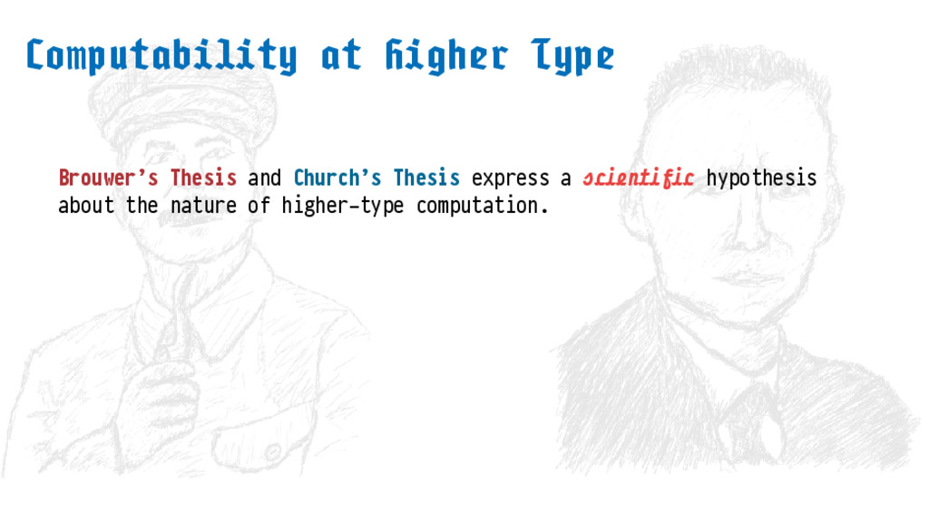
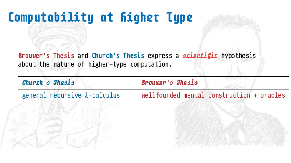
  65. Brouwer’s Thesis and Church’s Thesis express a hypothesis about the

    nature of higher-type computation. ' ' general recursive -calculus wellfounded mental construction + oracles
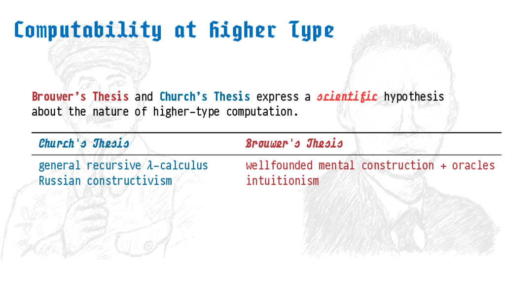
  66. Brouwer’s Thesis and Church’s Thesis express a hypothesis about the

    nature of higher-type computation. ' ' general recursive -calculus wellfounded mental construction + oracles Russian constructivism intuitionism
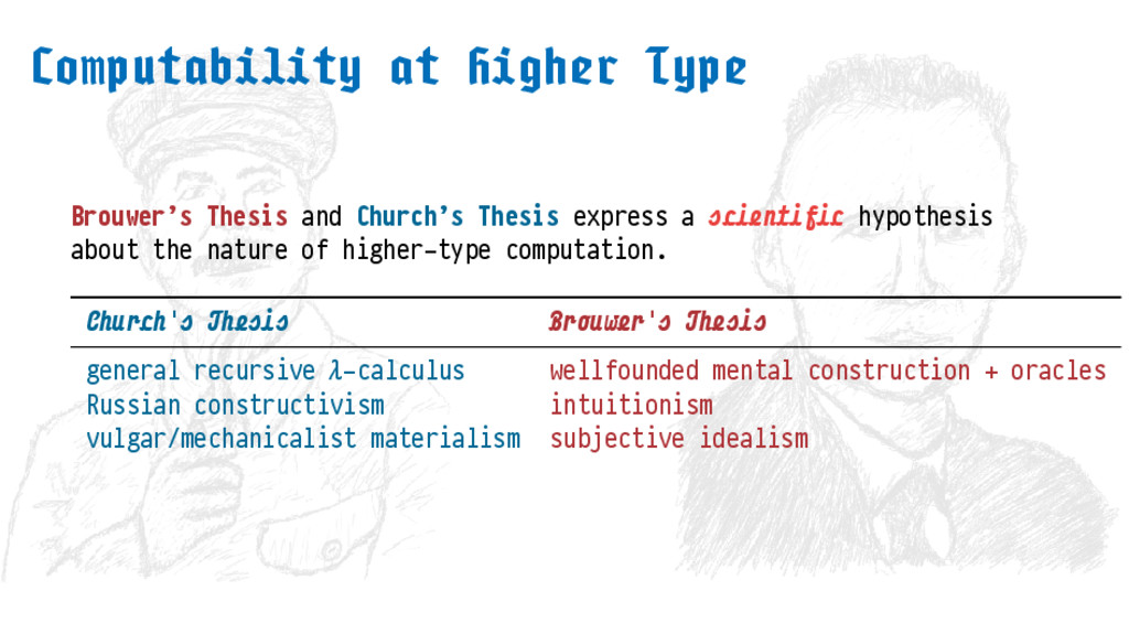
  67. Brouwer’s Thesis and Church’s Thesis express a hypothesis about the

    nature of higher-type computation. ' ' general recursive -calculus wellfounded mental construction + oracles Russian constructivism intuitionism vulgar/mechanicalist materialism subjective idealism
  68. Brouwer’s Thesis and Church’s Thesis express a hypothesis about the

    nature of higher-type computation. ' ' general recursive -calculus wellfounded mental construction + oracles Russian constructivism intuitionism vulgar/mechanicalist materialism subjective idealism uniform continuity fails on uniform continuity obtains