Simple rules for building robust machine learning models

Sixteen (16) simple rules for building robust machine learning models. Invited talk for the AMA call of the Research Data Alliance (RDA) Early Career and Engagement Interest Group (ECEIG).

Transcript

1. SIMPLE RULES FOR BUILDING ROBUST MACHINE LEARNING MODELS WITH EXAMPLES IN R Kyriakos Chatzidimitriou Research Fellow, Aristotle University of Thessaloniki PhD in Electrical and Computer Engineering kyrcha@issel.ee.auth.gr AMA Call Early Career and Engagement IG
2. ABOUT ME • Born in 1978 • 1997-2003, Diploma in Electrical and Computer Engineering, AUTH, GREECE • 2003-2004, Worked as a developer • 2004-2006, MSc in Computer Science, CSU, USA • 2006-2007, Greek Army • 2007-2012, PhD, AUTH, GREECE • Reinforcement learning and evolutionary computing mechanisms for autonomous agents • 2013-Now, Research Fellow, ECE, AUTH • 2017-Now, co-founder, manager and full stack developer of Cyclopt P.C. • Spin-off company of AUTH focusing on software analytics
3. GENERAL CAREER ADVICE Life is hard and full of problems. No point thus in meaningless suffering J To be happy and for the problems you can choose, choose those that you like solving. By working on the 10K hour of more… …you will be too good to be ignored and you will achieve that by focusing on deep work and working on difficult problems Positive feedback loop, where good things happen
4. WHAT IS ML (SUPERVISED)
5. WHAT AM I WORKING ON ML WISE Deep website aesthetics AutoML Continuous Implicit Authentication Formatting or linting errors
6. SIMPLE RULE 1: SPLIT YOU DATA IN THREE
7. GREEK SONG • «Δεν υπάρχει ευτυχία, που να κόβεται στα τρία…» – “There is no happiness split in three…” • Not true for ML
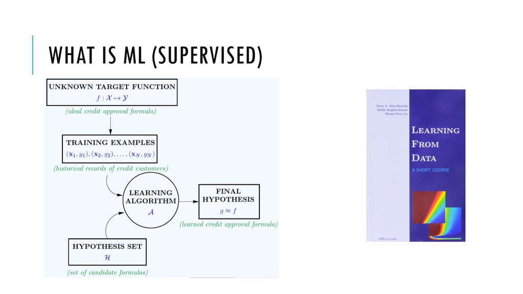
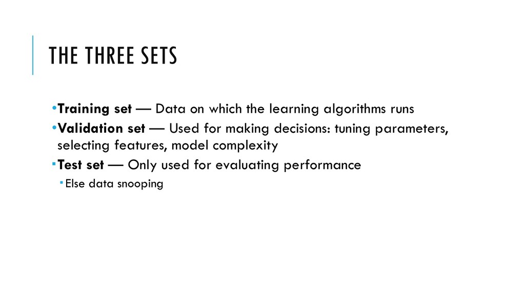
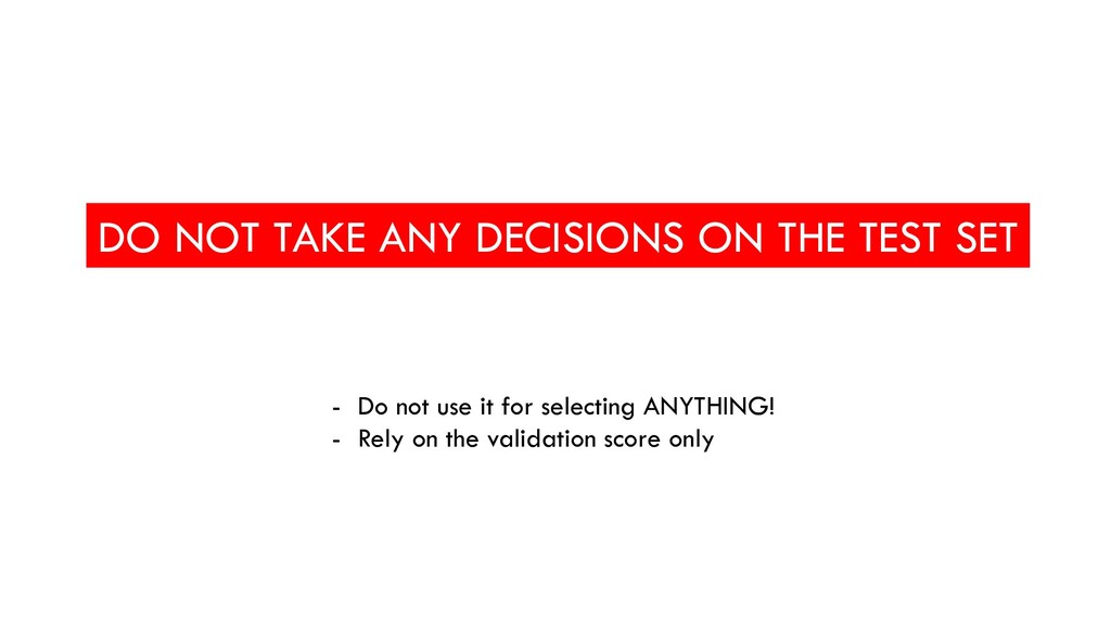
8. THE THREE SETS •Training set — Data on which the learning algorithms runs •Validation set — Used for making decisions: tuning parameters, selecting features, model complexity ­Test set — Only used for evaluating performance ­ Else data snooping
9. DO NOT TAKE ANY DECISIONS ON THE TEST SET - Do not use it for selecting ANYTHING! - Rely on the validation score only
10. VISUAL EXAMPLES OF SPLITS Whole Dataset Training Val Test 1F 2F 3F 4F 5F 6F 7F 8F 9F 10F Test Test 60-20-20 split 10-CV LOOCV
11. R EXAMPLE k = 5 results <- numeric(k) ind <- sample(2, nrow(iris), replace=T, prob=c(0.8, 0.2)) trainval <- iris[ind==1,] test <- iris[ind !=1,] cv <- sample(rep(1:k, length.out=nrow(trainval))) for(i in 1:k) { trainData <- trainval[cv != i,] valData <- trainval[cv == i,] model <- naiveBayes(Species ~ ., data=trainData, laplace = 0) pred <- predict(model, valData) results[i] <- Accuracy(pred, valData$Species) } print(mean(results)) # after finding the best laplace finalmodel <- naiveBayes(Species ~ ., data=trainval, laplace = 0) pred <- predict(finalmodel, test) print(Accuracy(pred, test$Species)) Validation - 0.95 vs. 0.91 - Test
12. SIMPLE RULE 2: SPLIT YOUR DATA IN THREE, CORRECTLY
13. 1948 US ELECTIONS 1948, Truman vs. Dewey Newspaper made a phone poll the previous day Most of Dewey supporters had phones those days
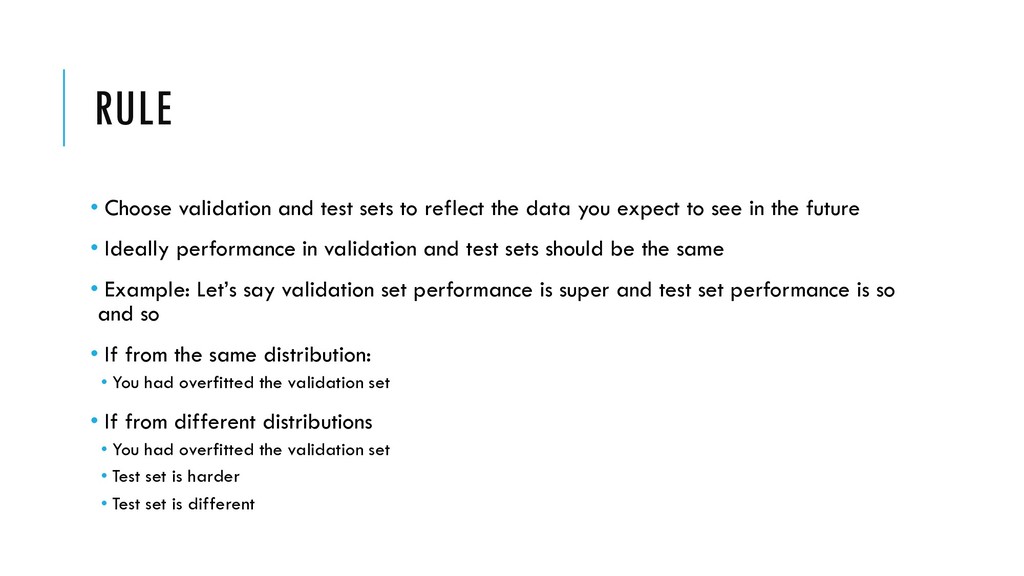
14. RULE • Choose validation and test sets to reflect the data you expect to see in the future • Ideally performance in validation and test sets should be the same • Example: Let’s say validation set performance is super and test set performance is so and so • If from the same distribution: • You had overfitted the validation set • If from different distributions • You had overfitted the validation set • Test set is harder • Test set is different
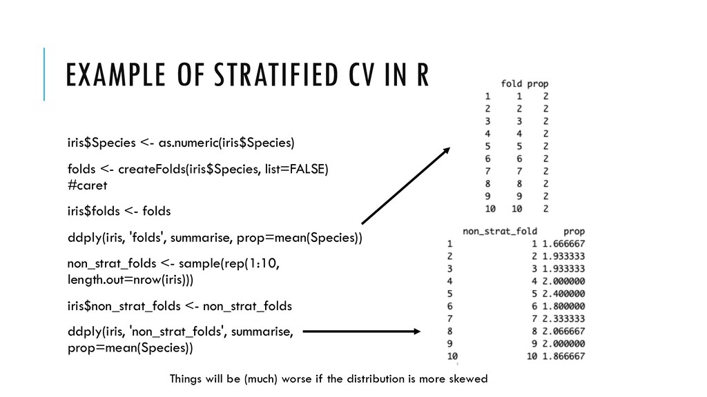
15. EXAMPLE OF STRATIFIED CV IN R iris$Species <- as.numeric(iris$Species) folds <- createFolds(iris$Species, list=FALSE) #caret iris$folds <- folds ddply(iris, 'folds', summarise, prop=mean(Species)) non_strat_folds <- sample(rep(1:10, length.out=nrow(iris))) iris$non_strat_folds <- non_strat_folds ddply(iris, 'non_strat_folds', summarise, prop=mean(Species)) Things will be (much) worse if the distribution is more skewed
16. SIMPLE RULE 3: DATASET SIZE IS IMPORTANT
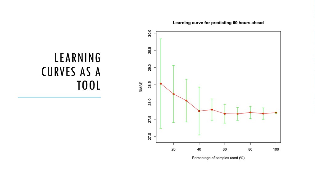
17. SIZE HEURISTICS • #1 Good validation set sizes are between 1000 and 10K • #2 For the training set have at least 10x the VC-dimension • For a NN is roughly equal to the number of weights • #3 Popular heuristic for test size should be 30%, less for large problems • #4 If you have more data, put them in the validation set to reduce overfitting • #5 The validation set should be large enough to detect differences between algorithms • For distinguishing between classifier A with 90% accuracy and B with 90.1% accuracy then 100 validation examples will not do it.
18. FINANCIAL IMPACT OF 0.1% Before 10,000,000 searches 1% CTR 100,000 visitors 1% conversion 1,000 purchases $100 $100,000 After 10,000,000 searches 1.1% CTR 110,000 visitors 1.1% conversion 1,210 purchases $100 $121,000 +$21,000 Bid Prediction Adaptive Content
19. LEARNING CURVES AS A TOOL
20. SIMPLE RULE 4: CHOOSE ONE METRIC
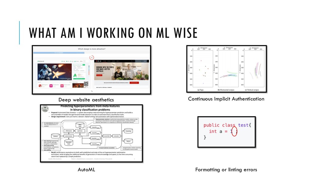
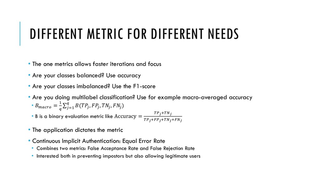
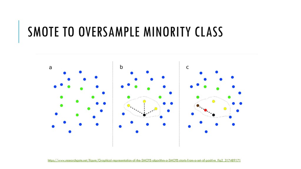
21. DIFFERENT METRIC FOR DIFFERENT NEEDS • The one metrics allows faster iterations and focus • Are your classes balanced? Use accuracy • Are your classes imbalanced? Use the F1-score • Are you doing multilabel classification? Use for example macro-averaged accuracy • "#$%& = ( ) ∑ +,( ) (+ , + , + , + ) • B is a binary evaluation metric like Accuracy = :;<=:>< :;<=?;<=:><=?>< • The application dictates the metric • Continuous Implicit Authentication: Equal Error Rate • Combines two metrics: False Acceptance Rate and False Rejection Rate • Interested both in preventing impostors but also allowing legitimate users
22. SIMPLE RULE 5: ALWAYS DO YOUR EDA
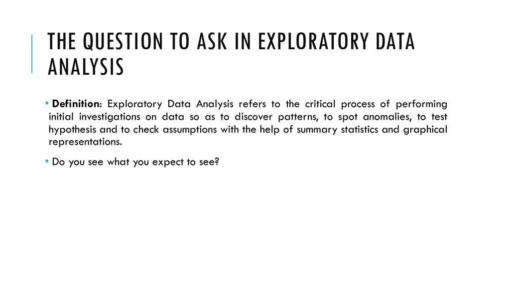
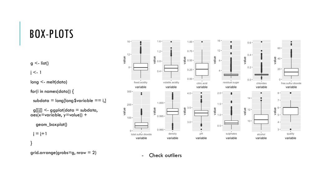
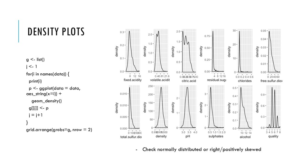
23. THE QUESTION TO ASK IN EXPLORATORY DATA ANALYSIS • Definition: Exploratory Data Analysis refers to the critical process of performing initial investigations on data so as to discover patterns, to spot anomalies, to test hypothesis and to check assumptions with the help of summary statistics and graphical representations. • Do you see what you expect to see?
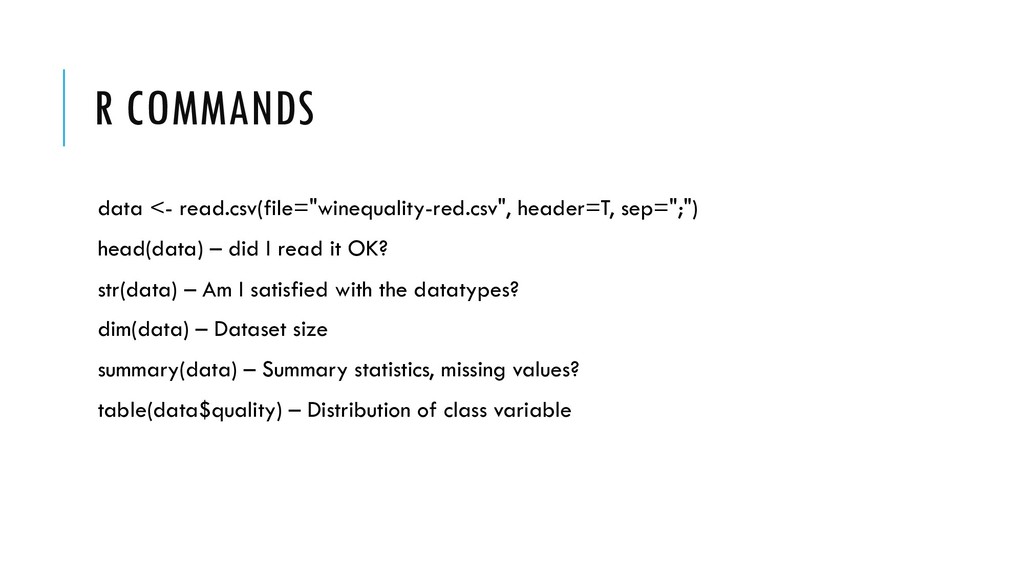
24. R COMMANDS data <- read.csv(file="winequality-red.csv", header=T, sep=";") head(data) – did I read it OK? str(data) – Am I satisfied with the datatypes? dim(data) – Dataset size summary(data) – Summary statistics, missing values? table(data$quality) – Distribution of class variable
25. CORRPLOT(W, METHOD="CIRCLE", TL.COL="BLACK", TL.SRT=45) install.packages(“corrplot”) - Check if correlations make sense. - Decide on dropping uncorrelated Variables with the class
26. BOX-PLOTS g <- list() j <- 1 long <- melt(data) for(i in names(data)) { subdata = long[long$variable == i,] g[[j]] <- ggplot(data = subdata, aes(x=variable, y=value)) + geom_boxplot() j = j+1 } grid.arrange(grobs=g, nrow = 2) - Check outliers
27. DENSITY PLOTS g <- list() j <- 1 for(i in names(data)) { print(i) p <- ggplot(data = data, aes_string(x=i)) + geom_density() g[[j]] <- p j = j+1 } grid.arrange(grobs=g, nrow = 2) - Check normally distributed or right/positively skewed
28. SIMPLE RULE 6: BE CAREFUL WITH DATA PREPROCESSING AS WELL
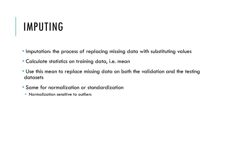
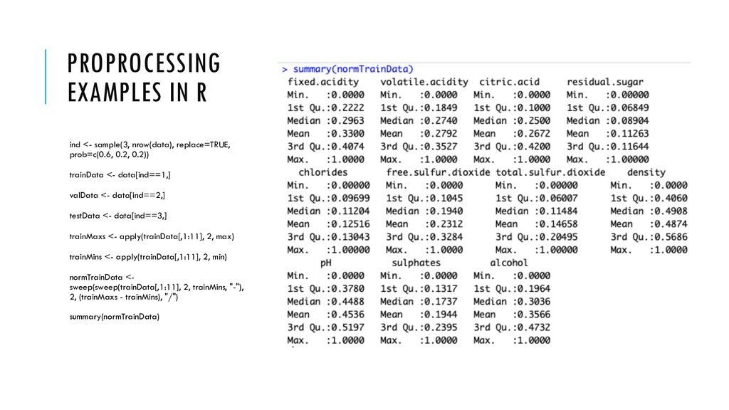
29. IMPUTING • Imputation: the process of replacing missing data with substituting values • Calculate statistics on training data, i.e. mean • Use this mean to replace missing data on both the validation and the testing datasets • Same for normalization or standardization • Normalization sensitive to outliers
30. PROPROCESSING EXAMPLES IN R ind <- sample(3, nrow(data), replace=TRUE, prob=c(0.6, 0.2, 0.2)) trainData <- data[ind==1,] valData <- data[ind==2,] testData <- data[ind==3,] trainMaxs <- apply(trainData[,1:11], 2, max) trainMins <- apply(trainData[,1:11], 2, min) normTrainData <- sweep(sweep(trainData[,1:11], 2, trainMins, "-"), 2, (trainMaxs - trainMins), "/") summary(normTrainData)
31. PROPROCESSING EXAMPLES IN R normValData <- sweep(sweep(valData[,1:11], 2, trainMins, "-"), 2, (trainMaxs - trainMins), "/") Not an issue if data is big and correct sampling is kept.
32. SIMPLE RULE 7: DON’T BE UNLUCKY
33. BE KNOWLEDGEABLE • Aka how randomness affects results… • If you don’t want to be unlucky do 10 times the 10-fold cross-validation and average the averages and get precise estimates
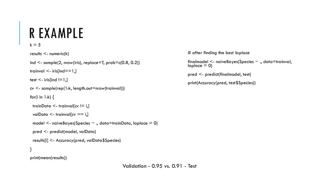
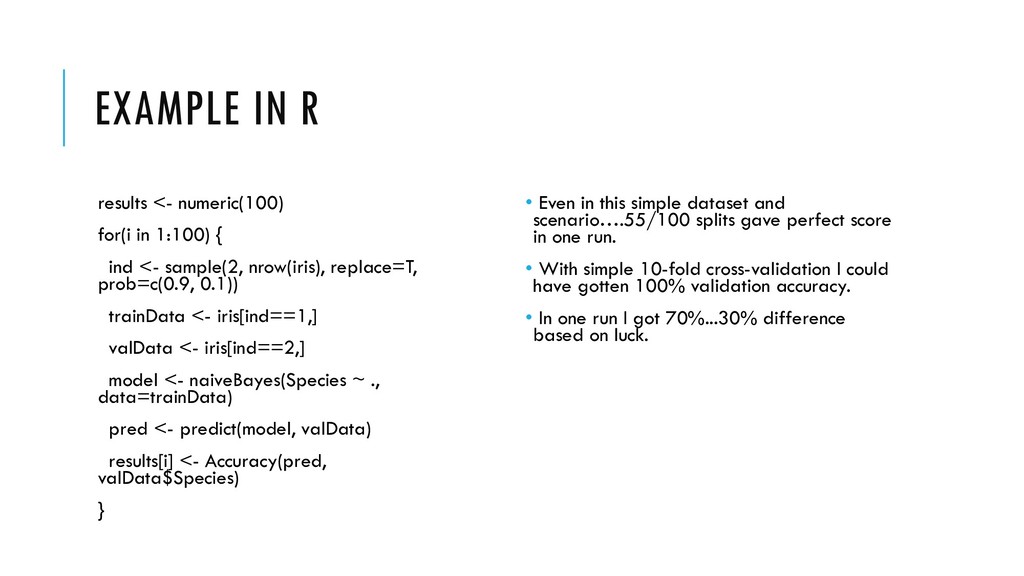
34. EXAMPLE IN R results <- numeric(100) for(i in 1:100) { ind <- sample(2, nrow(iris), replace=T, prob=c(0.9, 0.1)) trainData <- iris[ind==1,] valData <- iris[ind==2,] model <- naiveBayes(Species ~ ., data=trainData) pred <- predict(model, valData) results[i] <- Accuracy(pred, valData$Species) } • Even in this simple dataset and scenario….55/100 splits gave perfect score in one run. • With simple 10-fold cross-validation I could have gotten 100% validation accuracy. • In one run I got 70%...30% difference based on luck.
35. SIMPLE RULE 8: TESTING
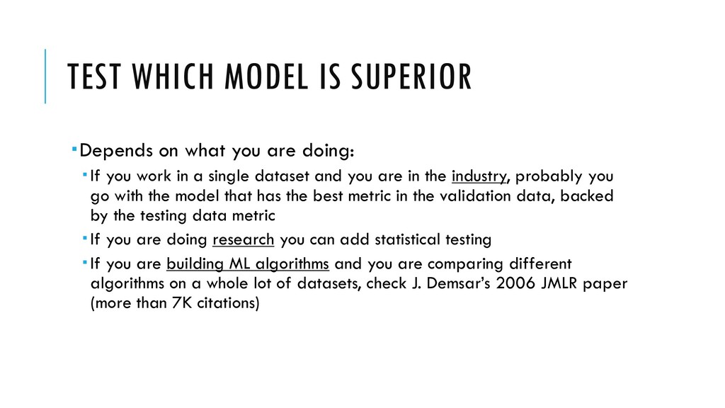
36. TEST WHICH MODEL IS SUPERIOR ­Depends on what you are doing: ­ If you work in a single dataset and you are in the industry, probably you go with the model that has the best metric in the validation data, backed by the testing data metric ­ If you are doing research you can add statistical testing ­ If you are building ML algorithms and you are comparing different algorithms on a whole lot of datasets, check J. Demsar’s 2006 JMLR paper (more than 7K citations)
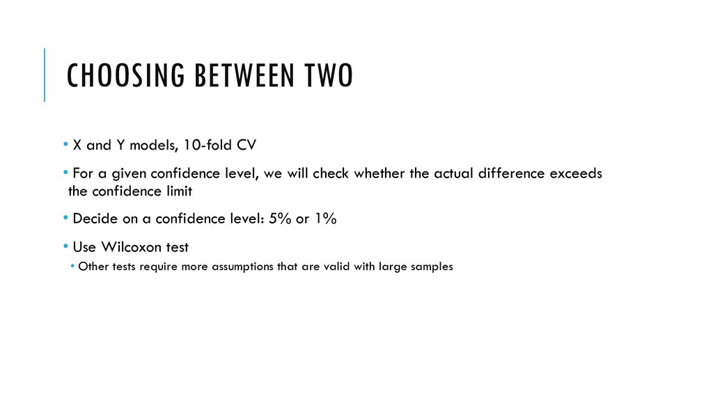
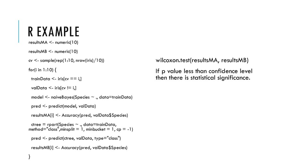
37. CHOOSING BETWEEN TWO • X and Y models, 10-fold CV • For a given confidence level, we will check whether the actual difference exceeds the confidence limit • Decide on a confidence level: 5% or 1% • Use Wilcoxon test • Other tests require more assumptions that are valid with large samples
38. R EXAMPLE resultsMA <- numeric(10) resultsMB <- numeric(10) cv <- sample(rep(1:10, nrow(iris)/10)) for(i in 1:10) { trainData <- iris[cv == i,] valData <- iris[cv != i,] model <- naiveBayes(Species ~ ., data=trainData) pred <- predict(model, valData) resultsMA[i] <- Accuracy(pred, valData$Species) ctree = rpart(Species ~ ., data=trainData, method="class",minsplit = 1, minbucket = 1, cp = -1) pred <- predict(ctree, valData, type="class") resultsMB[i] <- Accuracy(pred, valData$Species) } wilcoxon.test(resultsMA, resultsMB) If p value less than confidence level then there is statistical significance.
39. SIMPLE RULE 9: TIME IS MONEY
40. TIME IS MONEY • Before doing the whole experimentation, play with a small(er) dataset • What should this data be? • Representative!!! • Check all the pipeline, end-to-end GPU instances
41. SIMPLE RULE 10: KNOW THY DATA
42. DO I HAVE ENOUGH DATA? • Learning curves…. • Else augment • How can one augment?
43. IMAGE AUGMENTATION https://github.com/aleju/imgaug
44. SMOTE TO OVERSAMPLE MINORITY CLASS https://www.researchgate.net/figure/Graphical-representation-of-the-SMOTE-algorithm-a-SMOTE-starts-from-a-set-of-positive_fig2_317489171
45. MORE ANNOTATIONS
46. SIMPLE RULE 11: DECIDE ON YOUR GOAL
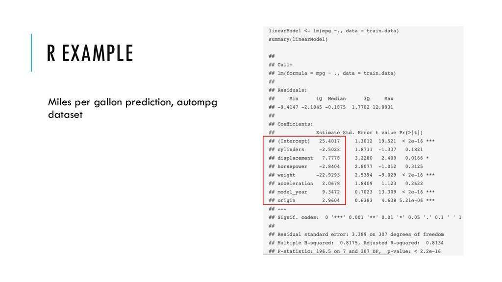
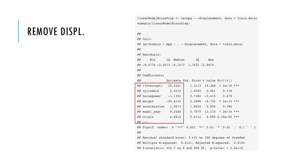
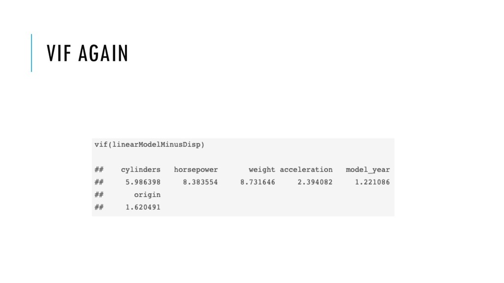
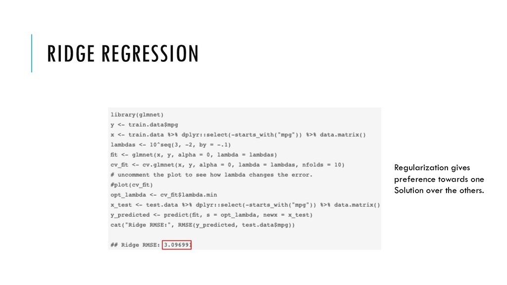
47. IS IT INTERPRETABILITY OR PERFORMANCE? • Decide what are you striving for. • (Multi)-Collinearity • X1 = a * X2 + b • Many different values of the features could predict equally well Y • Variance Inflation Factor (VIF) test • 1, no collinearity • >10, indication of collinearity • Discussed in: http://kyrcha.info/2019/03/22/on-collinearity-and-feature-selection
48. R EXAMPLE Miles per gallon prediction, autompg dataset
49. VIF
50. REMOVE DISPL.
51. VIF AGAIN
52. COMPARISON
53. REMOVE ALL VIF>10
54. RIDGE REGRESSION Regularization gives preference towards one Solution over the others.
55. RESULTS
56. SIMPLE RULE 12: START BY CHOOSING THE CORRECT MODEL FOR YOUR PROBLEM
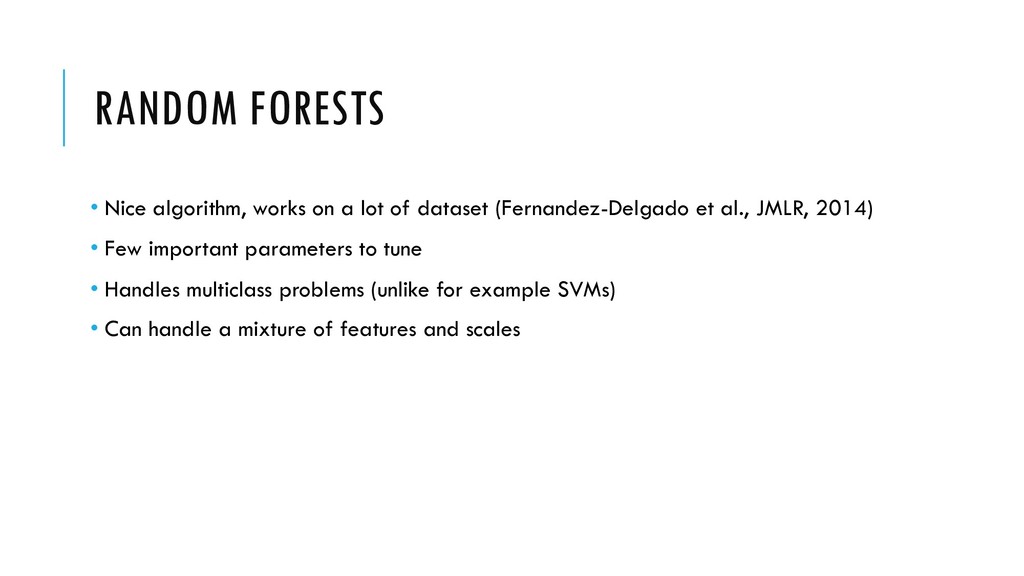
57. RANDOM FORESTS • Nice algorithm, works on a lot of dataset (Fernandez-Delgado et al., JMLR, 2014) • Few important parameters to tune • Handles multiclass problems (unlike for example SVMs) • Can handle a mixture of features and scales
58. SVM - Nice algorithm, works on a lot of dataset (Fernandez-Delgado et al., JMLR, 2014) - Robust theory behind it - Good for binary classification and 1-class classification ­ We use it in Continuous Implicit Authentication - Can handle sparse data
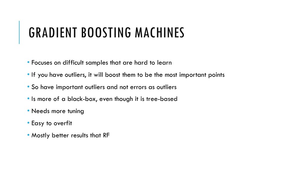
59. GRADIENT BOOSTING MACHINES • Focuses on difficult samples that are hard to learn • If you have outliers, it will boost them to be the most important points • So have important outliers and not errors as outliers • Is more of a black-box, even though it is tree-based • Needs more tuning • Easy to overfit • Mostly better results that RF
60. DEEP LEARNING • Choose if you have lots of data and computational resources • Don’t have to throw away anything. Solves the problem end-to-end.
61. SIDENOTE: BIAS - VARIANCE
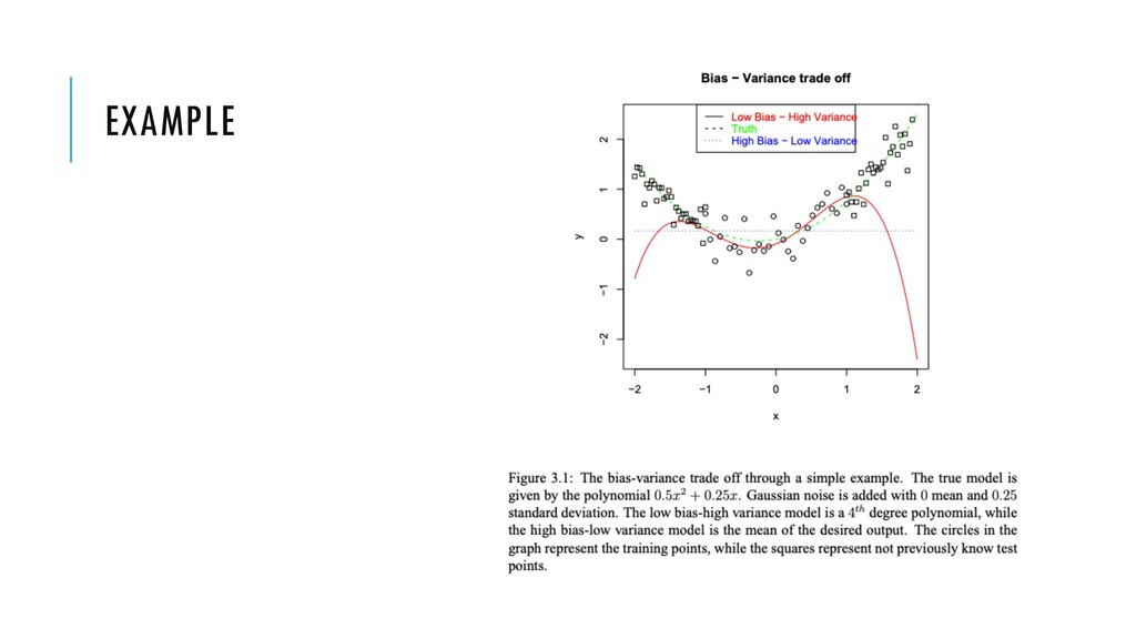
62. BIAS VS. VARIANCE Bias: algorithm’s error rate on the training set. Erroneous assumptions in the learning algorithm. Variance: difference in error rate between training set and validation set. It is caused by overfitting to the training data and accounting for small fluctuations. Learning from Data slides: http://work.caltech.edu/telecourse.html
63. EXAMPLE
64. SIMPLE RULE 13: BECOME A KNOWLEDGEABLE TRADER
65. BIAS VARIANCE TRADE-OFF HEURISTICS • #1 High bias => Increase model size (usually with regularization to mitigate high variance) • #2 High variance => add training data (usually with a big model to handle them)
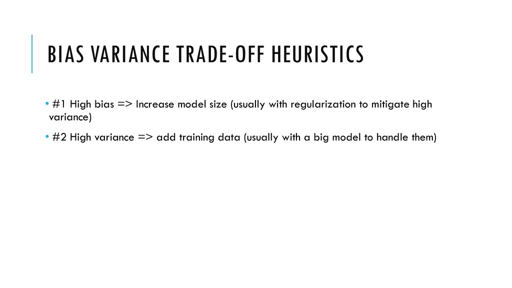
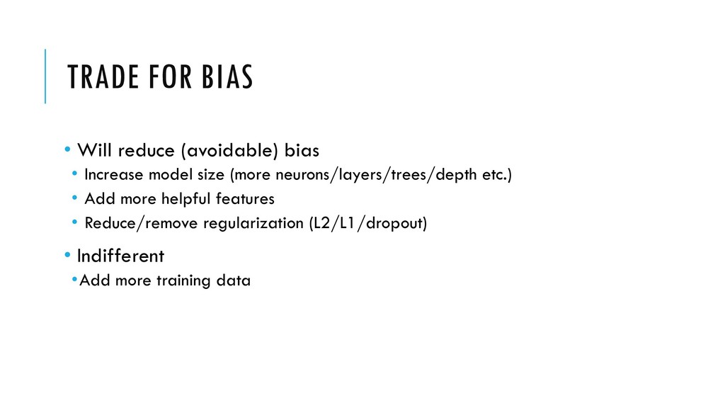
66. TRADE FOR BIAS • Will reduce (avoidable) bias • Increase model size (more neurons/layers/trees/depth etc.) • Add more helpful features • Reduce/remove regularization (L2/L1/dropout) • Indifferent •Add more training data
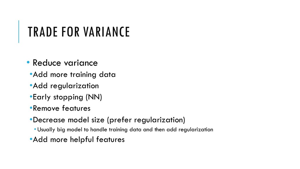
67. TRADE FOR VARIANCE • Reduce variance •Add more training data •Add regularization •Early stopping (NN) •Remove features •Decrease model size (prefer regularization) • Usually big model to handle training data and then add regularization •Add more helpful features
68. SIMPLE RULE 14: FINISH OFF WITH AN ENSEMBLE
69. ENSEMBLE TECHNIQUES - By now you’ve built a ton of models - Bagging: RF - Boosting: AdaBoost, GBT - Voting/Averaging - Stacking Classifier Classifier Classifier Classifier Classifier Final Prediction Predictions Training Data
70. SIMPLE RULE 15: TUNE HYPERPARAMETERS…BUT TO A POINT
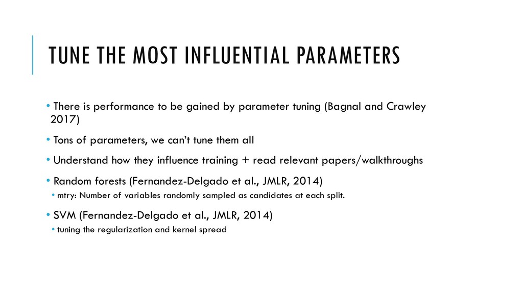
71. TUNE THE MOST INFLUENTIAL PARAMETERS • There is performance to be gained by parameter tuning (Bagnal and Crawley 2017) • Tons of parameters, we can’t tune them all • Understand how they influence training + read relevant papers/walkthroughs • Random forests (Fernandez-Delgado et al., JMLR, 2014) • mtry: Number of variables randomly sampled as candidates at each split. • SVM (Fernandez-Delgado et al., JMLR, 2014) • tuning the regularization and kernel spread
72. SIMPLE RULE 16: START A WATERFALL LIKE PROCESS
73. THE PROCESS Study the problem EDA Define optimization strategy (validation, test sets and metric) Feature Engineering Modelling Ensembling Error Analysis
74. GENERAL RULE
75. THE BASIC RECIPE (BY ANDREW NG) http://t.co/1Rn6q35Qf2
76. THANK YOU For further AMA questions open an issue at: https://github.com/kyrcha/ama
77. FURTHER READING • Personal Experiences • Various resources over the internet and the years • ML Yearning: https://www.mlyearning.org/ • Machine Learning from Data course: http://work.caltech.edu/telecourse.html • Practical Machine Learning with H2O book