L1 Monge Kantorovich problem with applications

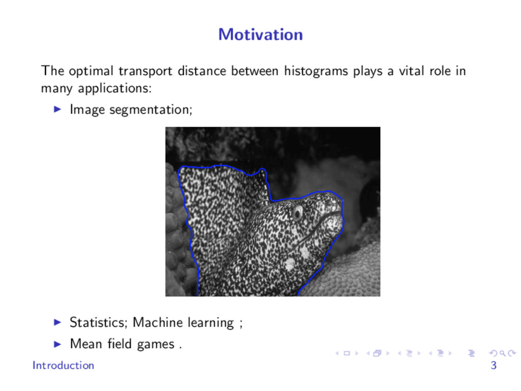
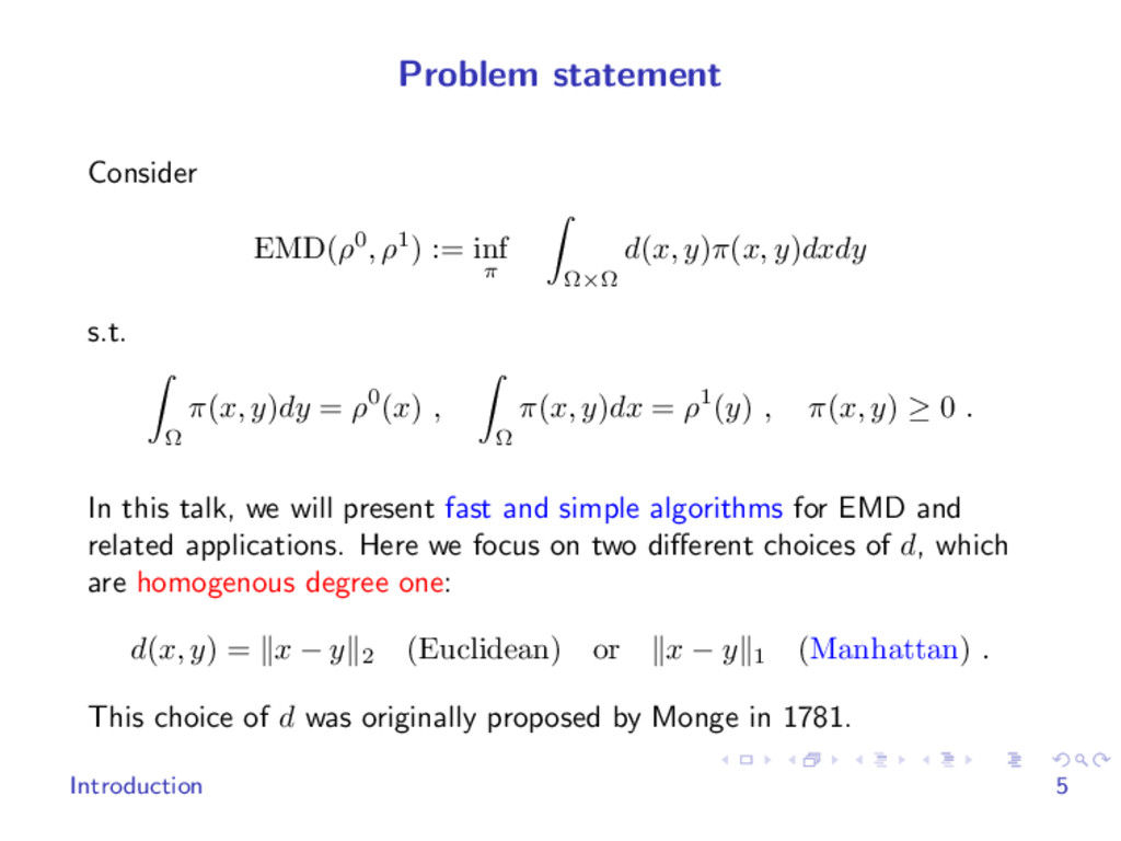
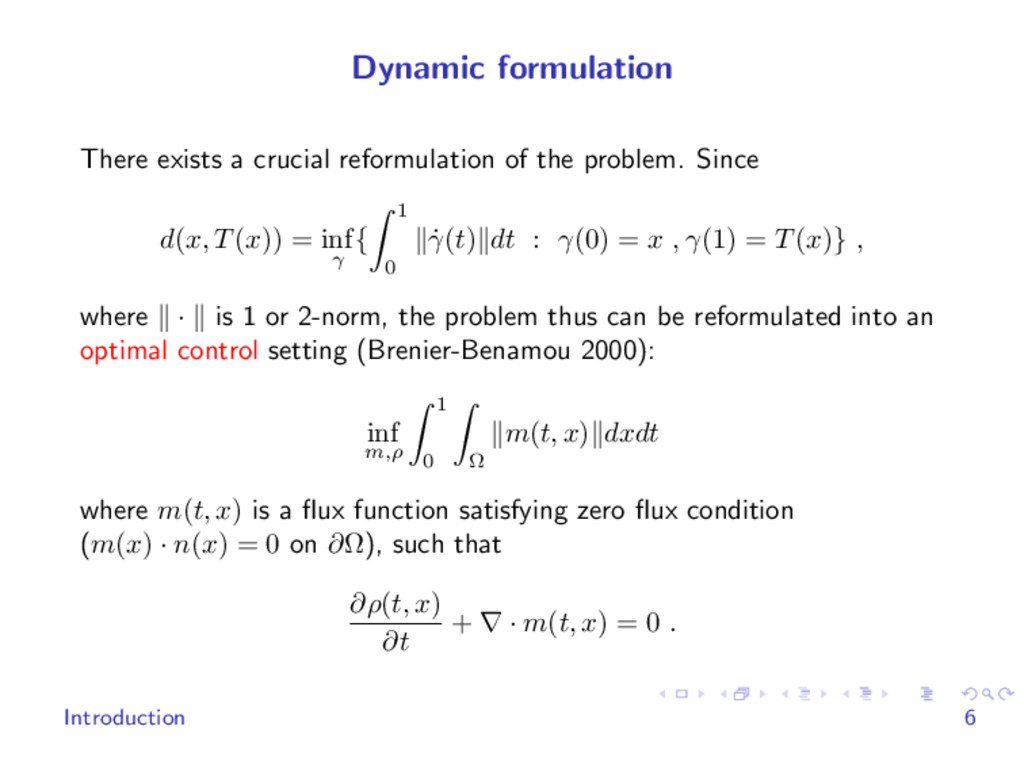
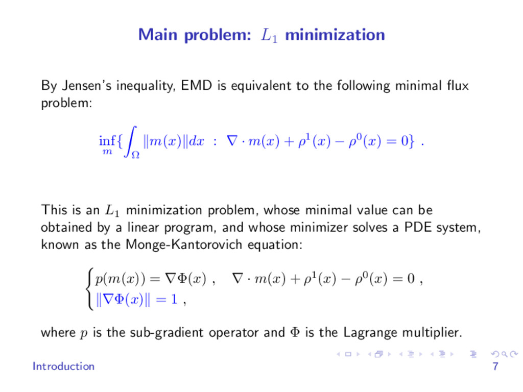
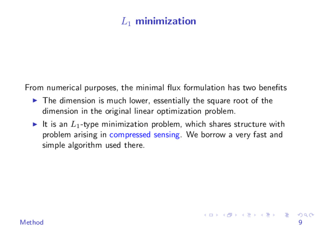
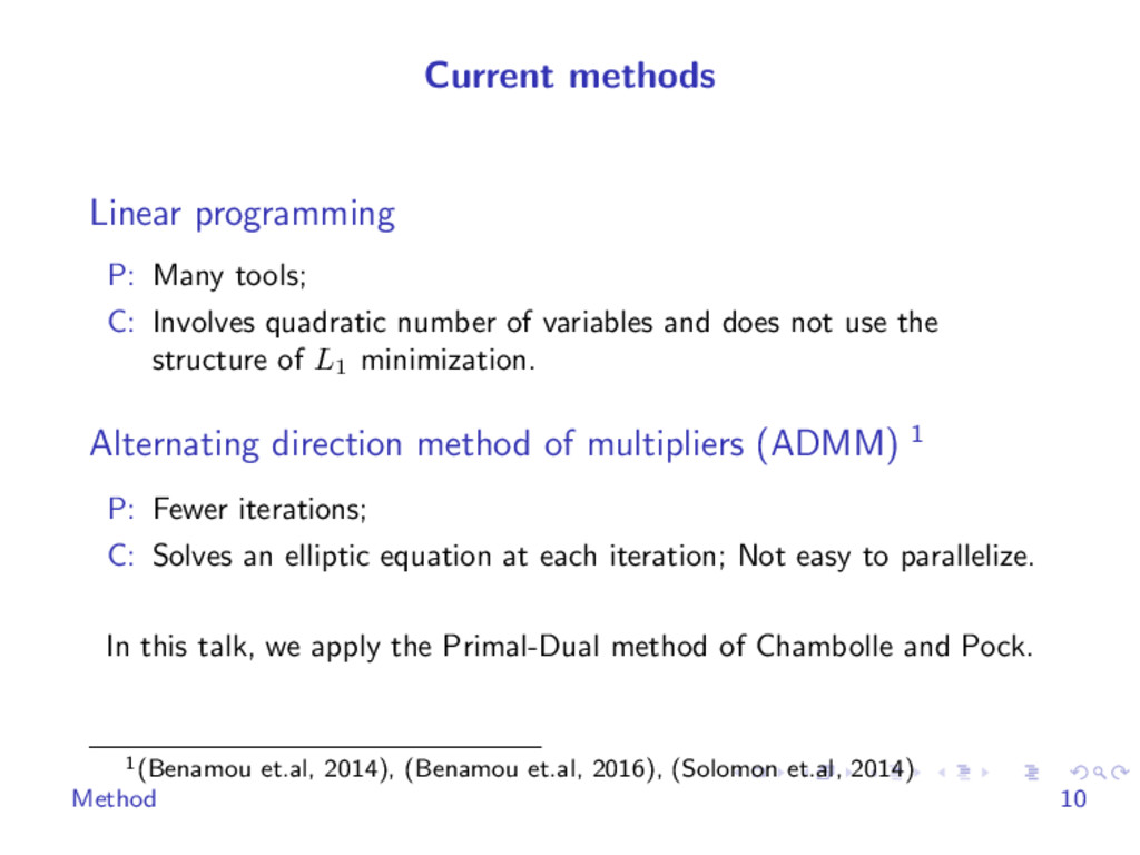
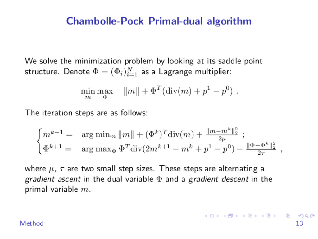
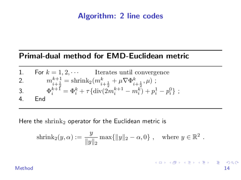
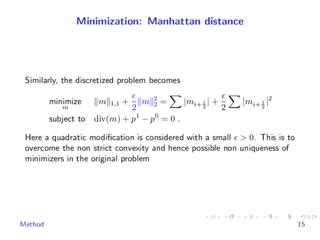
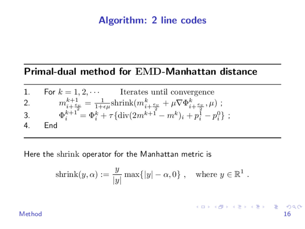
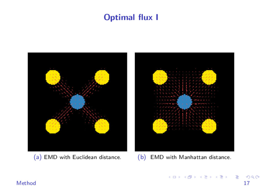
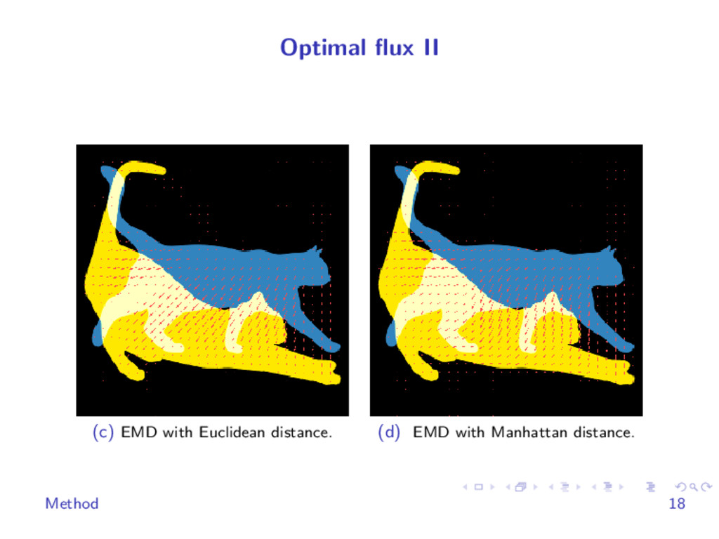
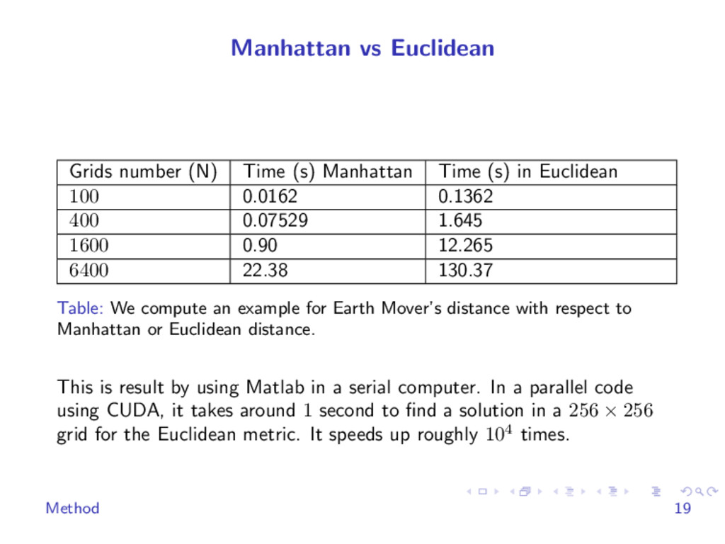
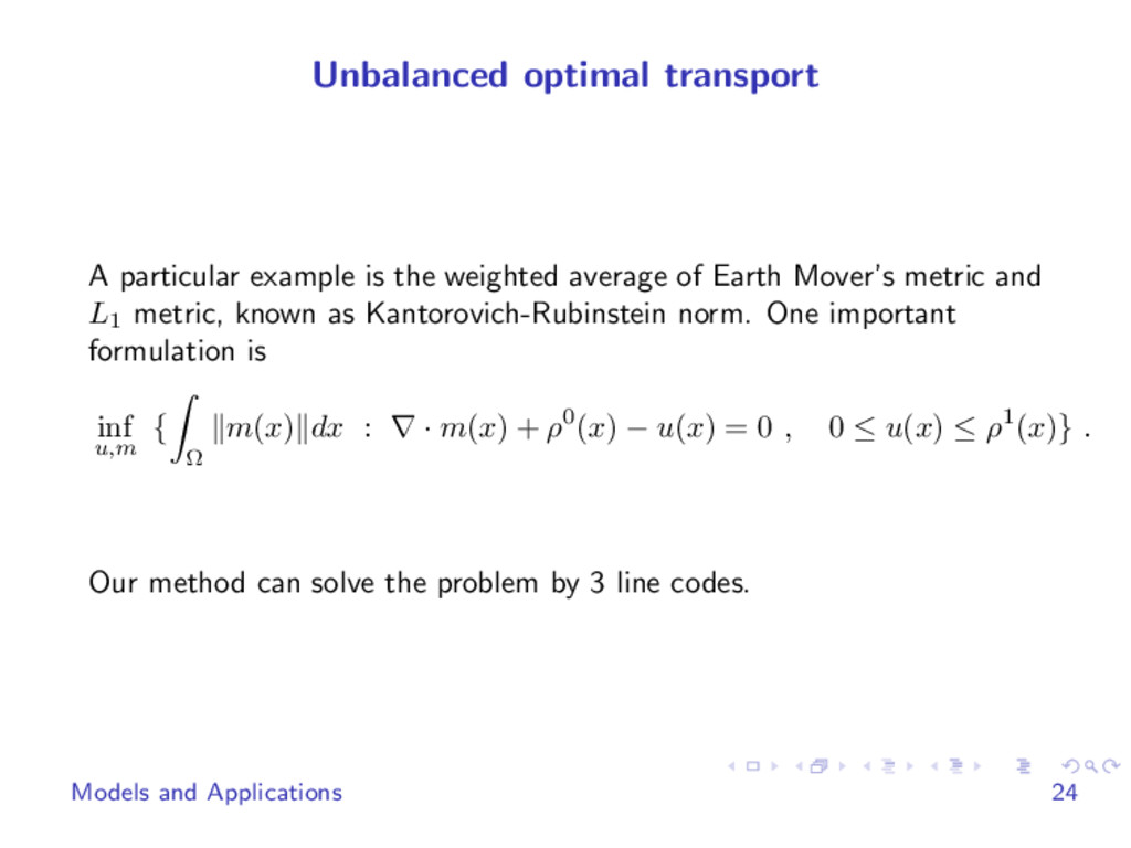
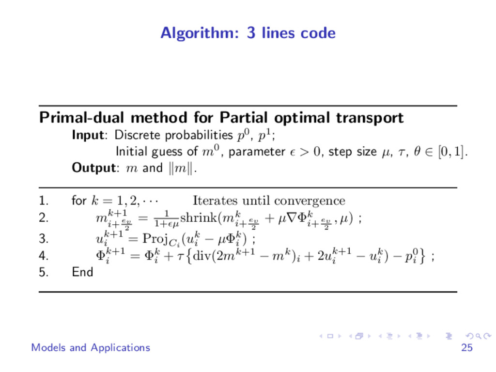
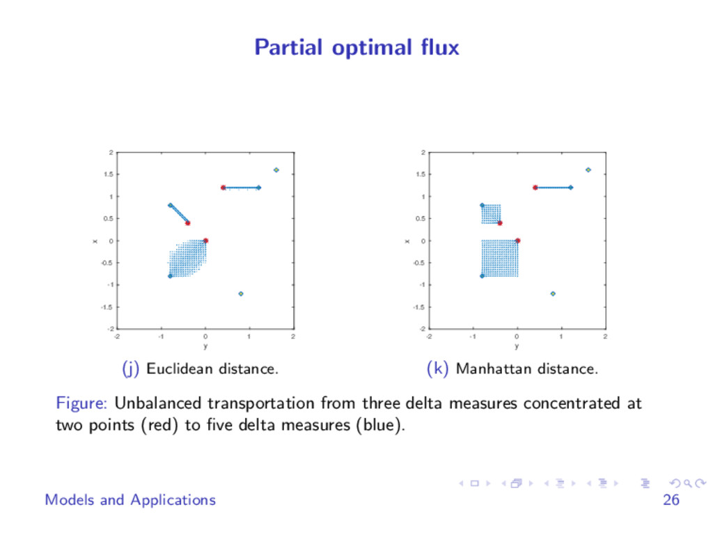
We develop fast methods for solving L1 Monge-Kantorovich type problems using techniques borrowed from fast algorithms for L1 regularized problems arising in compressive sensing. Our method is very simple, easy to parallelize and can be easily combined with other regularizations. We use it in applications including partial optimal transport, image segmentation, image alignment and others. It is flexible enough to easily deal with histograms and other features of the data.

Transcript

1. L1 Monge-Kantorovich problem with applications Wuchen Li UCLA June 3, 2017 Joint work with Stanley Osher, Wilfrid Gangbo, Wotao Yin, Ernest Ryu, Yupeng Li and Penghang Yin. Partially supported by ONR and DOE.
2. Outline Introduction Method Models and Applications Unbalanced optimal transport Image segmentation Introduction 2
3. Motivation The optimal transport distance between histograms plays a vital role in many applications: Image segmentation; Statistics; Machine learning ; Mean field games . Introduction 3
4. Earth Mover’s distance What is the optimal way to move (transport) some materials with shape X, density ρ0(x) to another shape Y with density ρ1(y)? The question leads to the definition of the Earth Mover’s distance (EMD), also called the Wasserstein metric, or the Monge-Kantorovich problem. Introduction 4
5. Problem statement Consider EMD(ρ0, ρ1) := inf π Ω×Ω d(x, y)π(x, y)dxdy s.t. Ω π(x, y)dy = ρ0(x) , Ω π(x, y)dx = ρ1(y) , π(x, y) ≥ 0 . In this talk, we will present fast and simple algorithms for EMD and related applications. Here we focus on two different choices of d, which are homogenous degree one: d(x, y) = x − y 2 (Euclidean) or x − y 1 (Manhattan) . This choice of d was originally proposed by Monge in 1781. Introduction 5
6. Dynamic formulation There exists a crucial reformulation of the problem. Since d(x, T(x)) = inf γ { 1 0 ˙ γ(t) dt : γ(0) = x , γ(1) = T(x)} , where · is 1 or 2-norm, the problem thus can be reformulated into an optimal control setting (Brenier-Benamou 2000): inf m,ρ 1 0 Ω m(t, x) dxdt where m(t, x) is a flux function satisfying zero flux condition (m(x) · n(x) = 0 on ∂Ω), such that ∂ρ(t, x) ∂t + ∇ · m(t, x) = 0 . Introduction 6
7. Main problem: L1 minimization By Jensen’s inequality, EMD is equivalent to the following minimal flux problem: inf m { Ω m(x) dx : ∇ · m(x) + ρ1(x) − ρ0(x) = 0} . This is an L1 minimization problem, whose minimal value can be obtained by a linear program, and whose minimizer solves a PDE system, known as the Monge-Kantorovich equation: p(m(x)) = ∇Φ(x) , ∇ · m(x) + ρ1(x) − ρ0(x) = 0 , ∇Φ(x) = 1 , where p is the sub-gradient operator and Φ is the Lagrange multiplier. Introduction 7
8. Outline Introduction Method Models and Applications Unbalanced optimal transport Image segmentation Method 8
9. L1 minimization From numerical purposes, the minimal flux formulation has two benefits The dimension is much lower, essentially the square root of the dimension in the original linear optimization problem. It is an L1 -type minimization problem, which shares structure with problem arising in compressed sensing. We borrow a very fast and simple algorithm used there. Method 9
10. Current methods Linear programming P: Many tools; C: Involves quadratic number of variables and does not use the structure of L1 minimization. Alternating direction method of multipliers (ADMM) 1 P: Fewer iterations; C: Solves an elliptic equation at each iteration; Not easy to parallelize. In this talk, we apply the Primal-Dual method of Chambolle and Pock. 1(Benamou et.al, 2014), (Benamou et.al, 2016), (Solomon et.al, 2014) Method 10
11. Settings Introduce a uniform grid G = (V, E) with spacing ∆x to discretize the spatial domain, where V is the vertex set and E is the edge set. i = (i1 , · · · , id ) ∈ V represents a point in Rd. Consider a discrete probability set supported on all vertices: P(G) = {(pi )N i=1 ∈ RN | N i=1 pi = 1 , pi ≥ 0 , i ∈ V } , and a discrete flux function defined on the edge of G : mi+ 1 2 = (mi+ 1 2 ev )d v=1 , where mi+ 1 2 ev represents a value on the edge (i, i + ev ) ∈ E, ev = (0, · · · , ∆x, · · · , 0)T , ∆x is at the v-th column. Method 11
12. Minimization: Euclidean distance We first consider EMD with the Euclidean distance. The discretized problem becomes minimize m m 1,2 subject to div(m) + p1 − p0 = 0 , which can be formulated explicitly minimize m N i=1 d v=1 |mi+ 1 2 ev |2 subject to 1 ∆x d v=1 (mi+ 1 2 ev − mi− 1 2 ev ) + p1 i − p0 i = 0 . Method 12
13. Chambolle-Pock Primal-dual algorithm We solve the minimization problem by looking at its saddle point structure. Denote Φ = (Φi )N i=1 as a Lagrange multiplier: min m max Φ m + ΦT (div(m) + p1 − p0) . The iteration steps are as follows: mk+1 = arg minm m + (Φk)T div(m) + m−mk 2 2 2µ ; Φk+1 = arg maxΦ ΦT div(2mk+1 − mk + p1 − p0) − Φ−Φk 2 2 2τ , where µ, τ are two small step sizes. These steps are alternating a gradient ascent in the dual variable Φ and a gradient descent in the primal variable m. Method 13
14. Algorithm: 2 line codes Primal-dual method for EMD-Euclidean metric 1. For k = 1, 2, · · · Iterates until convergence 2. mk+1 i+ 1 2 = shrink2 (mk i+ 1 2 + µ∇Φk i+ 1 2 , µ) ; 3. Φk+1 i = Φk i + τ{div(2mk+1 i − mk i ) + p1 i − p0 i } ; 4. End Here the shrink2 operator for the Euclidean metric is shrink2 (y, α) := y y 2 max{ y 2 − α, 0} , where y ∈ R2 . Method 14
15. Minimization: Manhattan distance Similarly, the discretized problem becomes minimize m m 1,1 + 2 m 2 2 = |mi+ 1 2 | + 2 |mi+ 1 2 |2 subject to div(m) + p1 − p0 = 0 . Here a quadratic modification is considered with a small > 0. This is to overcome the non strict convexity and hence possible non uniqueness of minimizers in the original problem Method 15
16. Algorithm: 2 line codes Primal-dual method for EMD-Manhattan distance 1. For k = 1, 2, · · · Iterates until convergence 2. mk+1 i+ ev 2 = 1 1+ µ shrink(mk i+ ev 2 + µ∇Φk i+ ev 2 , µ) ; 3. Φk+1 i = Φk i + τ{div(2mk+1 − mk)i + p1 i − p0 i } ; 4. End Here the shrink operator for the Manhattan metric is shrink(y, α) := y |y| max{|y| − α, 0} , where y ∈ R1 . Method 16
17. Optimal flux I (a) EMD with Euclidean distance. (b) EMD with Manhattan distance. Method 17
18. Optimal flux II (c) EMD with Euclidean distance. (d) EMD with Manhattan distance. Method 18
19. Manhattan vs Euclidean Grids number (N) Time (s) Manhattan Time (s) in Euclidean 100 0.0162 0.1362 400 0.07529 1.645 1600 0.90 12.265 6400 22.38 130.37 Table: We compute an example for Earth Mover’s distance with respect to Manhattan or Euclidean distance. This is result by using Matlab in a serial computer. In a parallel code using CUDA, it takes around 1 second to find a solution in a 256 × 256 grid for the Euclidean metric. It speeds up roughly 104 times. Method 19
20. Importance of (e) = 0. (f) = 0. (g) small. Two different minimizers above on left are for = 0. Method 20
21. PDEs behind It is worth mentioning that the minimizer of the regularized problem inf m { Ω m(x) + 2 m(x) 2dx : ∇ · m(x) + ρ1(x) − ρ0(x) = 0} , satisfies a nice (formal) system m(x) = 1 (∇Φ(x) − ∇Φ(x) |∇Φ(x)| ) , 1 (∆Φ(x) − ∇ · ∇Φ(x) |∇Φ(x)| ) = ρ0(x) − ρ1(x) , where the second equation holds when |∇Φ| ≥ 1. Notice that the term ∇ · ∇Φ(x) |∇Φ(x)| is the mean curvature formula. Method 21
22. Outline Introduction Method Models and Applications Unbalanced optimal transport Image segmentation Models and Applications 22
23. Unbalanced optimal transport The original problem assumes that the total mass of given densities should be equal, which often does not hold in practice. E.g. the intensities of two images can be different. Partial optimal transport seeks optimal plans between two measures ρ0, ρ1 with unbalanced masses, i.e. Ω ρ0(x)dx = Ω ρ1(y)dy . 100 80 60 40 20 0 0 50 1 0.8 0.6 0.4 0.2 0 100 (h) ρ0. 100 80 60 40 20 0 0 50 1 0 0.2 0.4 0.6 0.8 100 (i) ρ1. Models and Applications 23
24. Unbalanced optimal transport A particular example is the weighted average of Earth Mover’s metric and L1 metric, known as Kantorovich-Rubinstein norm. One important formulation is inf u,m { Ω m(x) dx : ∇ · m(x) + ρ0(x) − u(x) = 0 , 0 ≤ u(x) ≤ ρ1(x)} . Our method can solve the problem by 3 line codes. Models and Applications 24
25. Algorithm: 3 lines code Primal-dual method for Partial optimal transport Input: Discrete probabilities p0, p1; Initial guess of m0, parameter > 0, step size µ, τ, θ ∈ [0, 1]. Output: m and m . 1. for k = 1, 2, · · · Iterates until convergence 2. mk+1 i+ ev 2 = 1 1+ µ shrink(mk i+ ev 2 + µ∇Φk i+ ev 2 , µ) ; 3. uk+1 i = ProjCi (uk i − µΦk i ) ; 4. Φk+1 i = Φk i + τ div(2mk+1 − mk)i + 2uk+1 i − uk i ) − p0 i ; 5. End Models and Applications 25
26. Partial optimal flux y -2 -1 0 1 2 x -2 -1.5 -1 -0.5 0 0.5 1 1.5 2 (j) Euclidean distance. y -2 -1 0 1 2 x -2 -1.5 -1 -0.5 0 0.5 1 1.5 2 (k) Manhattan distance. Figure: Unbalanced transportation from three delta measures concentrated at two points (red) to five delta measures (blue). Models and Applications 26
27. Image segmentation Given a grey-value image I : Ω → R. The problem is to find two regions Ω1 , Ω2 , such that Ω1 ∪ Ω2 = Ω , Ω1 ∩ Ω2 = ∅. Idea of Mumford-Shah model: min Ω1,Ω2 λPer(Ω1 , Ω2 ) + Dist(Ω1 , a) + Dist(Ω2 , b) . where a, b are some given references generated by the image I(x), known as the supervised terms, and Dist is some functional which estimates the closeness between region and references. There are some famous models, such as Mumford-Shah, Chan-Vese, Chan, Ni et al. 2007, Rabin et al. 2017. Models and Applications 27
28. Orignal Monge-Kantorovich+ Segmentation It avoids overfitting of features (Swoboda and Schnorr (2003)); It is L1 minimization, which is great for computations. Given intensity I(x), the proposed model is: min u λ Ω |∇u(x)|dx + EMD(HI u, a) + Dist(HI (1 − u), b) , where u is the indicator function of region, HI is a linear operator depending on I which changes u into histograms, a, b are histograms in the selected red or blue regions: Models and Applications 28
29. Problem formulation inf u,m1,m2 λ Ω ∇x u(x) dx + F m1 (y) dy + F m2 (y) dy , where the infimum is taken among u(x) and flux functions m1 (y), m2 (y) satisfying              0 ≤ u(x) ≤ 1 ∇y · m1 (y) + HI (u)(y) − a(y) F HI (u)(y)dy = 0 ∇y · m2 (y) + HI (1 − u)(y) − b(y) F HI (1 − u)(y)dy = 0 . Here x ∈ Ω, y ∈ F, HI : BV(Ω) → Measure(F) is a linear operator. Our algorithm can be easily used into this area. It contains only 6 simple and explicit iterations using the Chamolle-Pock primal dual method. Models and Applications 29
30. Segmentation with multiple dimensional features (a) Histogram of intensity, Mean (b) Histogram of intensity, Mean, Texture We take λ = 1, the mean and texture (Sochen et. al) are values chosen in 3 × 3 patches near each pixel. Models and Applications 30
31. Segmentation with multiple dimensional features (c) Histogram of intensity, Mean (d) Histogram of intensity, Mean, Texture Models and Applications 31
32. Segmentation with multiple dimensional features (e) Histogram of intensity, Mean (f) Histogram of intensity, Mean, Texture Models and Applications 32
33. PDEs behind segmentation It is interesting to observe that there are three mean curvature formulas in both spatial and feature domains. Primal-Dual method avoids solving nonlinear PDEs directly!!! Models and Applications 33
34. Discussion Our method for solving L1 Monge-Kantorovich related problems handles the sparsity of histograms; has simple updates and is easy to parallelize; introduces a novel PDE system (Mean curvature formula in Monge Kantorovich equation). It has been successfully used in partial optimal transport, image segmentation, image alignment and elsewhere. Models and Applications 34
35. Main references Wuchen Li, Ernest Ryu, Stanley Osher, Wotao Yin and Wilfrid Gangbo. A parallel method for Earth Mover’s distance, 2016. Ernest Ryu, Wuchen Li, Penghang Yin and Stanley Osher. A Fast algorithm for unbalanced L1 Monge-Kantorovich problem, 2016. Yupeng Li, Wuchen Li and Stanley Osher. Image segmentation via original Monge-Kantorovich problem, in prepration. Models and Applications 35
36. Thanks! Models and Applications 36